Rules for Optical Metrology - NASA · PDF fileRules for Optical Metrology. H. Philip Stahl,...

Rules for Optical Metrology

H. Philip Stahl NASA Marshall Space Flight Center (MSFC), Huntsville, AL

Paper will define the four metrology rules used to test the James Webb Space Telescope (JWST) flight mirrors and give examples of how the rules were applied in practice.

International Commission for Optics: (ICO) 22 General Congress William O. Jenkings Convention Center in Puebla, Mexico

August 15 to 19, 2011

https://ntrs.nasa.gov/search.jsp?R=20110015786 2018-04-23T13:33:27+00:00Z

International Commission for Optics 22nd General Congress (2011)


H. Philip Stahl, PhD

NASA Marshall Space Flight Center, Huntsville, AL [email protected]

ABSTRACT Based on 30 years of optical testing experience, I have defined seven guiding principles for optical testing. This paper introduces these rules and discusses examples of their application.

Keywords: Optical Testing

1. INTRODUCTION Optical testing is the discipline of quantifying the performance parameters of an optical component or optical system using any appropriate metrology tool. By contrast, optical metrology is the discipline of quantifying parameters (typically physical but not necessarily) using optical techniques. By these definitions, I have over 30 years experience as an optical metrologist performing optical testing. My optical testing career started as a student at the Arizona Optical Sciences Center by taking ‘Optical Testing’ from Professor James C. Wyant. In 1982 I had a summer job with Fritz Zernike, Jr. at Perkin Elmer performing optical testing on microlithography components. My 1985 PhD dissertation involved the design and fabrication of an infrared phase-measuring interferometer using a pyroelectric vidicon1. I spent 5 years designing and building interferometers (infrared and visible) and writing phase-measuring interferometric software at Breault Research Organization (BRO). Arizona and REOSC both used my IR interferometers for testing their large telescope mirrors during early grinding and polishing. One of my most interesting efforts was the design and fabrication of a high-speed common-path interferometer which enabled the fabrication of the Keck primary mirror segments2. Next I spend 4 years teaching optical testing and optical metrology to undergraduate and graduate students at Rose-Hulman3,4. During this period I involved several of my students in an optical metrology project to measure the surface shape of a pool of liquid silicon in microgravity on the Space Shuttle5. It was not until 1993 that I actually got to practice the craft of optical testing in Danbury (Perkin Elmer, Hughes, Raytheon, now Goodrich). Danbury was an excellent experience. I learned much from my colleagues (particularly Joe Magner who had been doing optical testing since the 1960s) and from the projects on which I worked6,7,8. Since 1999 I have been responsible for development and overseeing the in-process optical testing and final certification testing of the James Webb Space Telescope (JWST) optical telescope element (OTE) optical components9,10,11,12

Based on my 30 years of optical testing experience, I have defined seven guiding principles for optical testing. This paper introduces these rules and discusses examples of their application.

.

2. GUIDING PRINCIPLES FOR OPTICAL TESTING No matter how small or large your optical testing task, the following simple principles will insure success:

1. Fully Understand the Task 2. Develop an Error Budget 3. Continuous Metrology Coverage 4. Know where you are 5. ‘Test like you fly’ 6. Independent Cross-Checks 7. Understand All Anomalies

These rules have been derived from my own failures and successes. And, these rules have been applied with great success to the in-process optical testing and final specification compliance testing of the JWST OTE mirrors.

mailto:[email protected]�


2.1 Fully Understand the Task

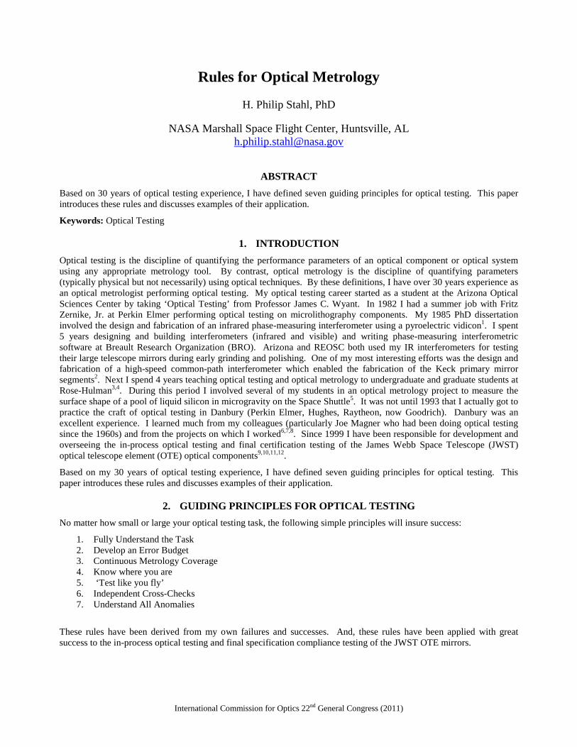
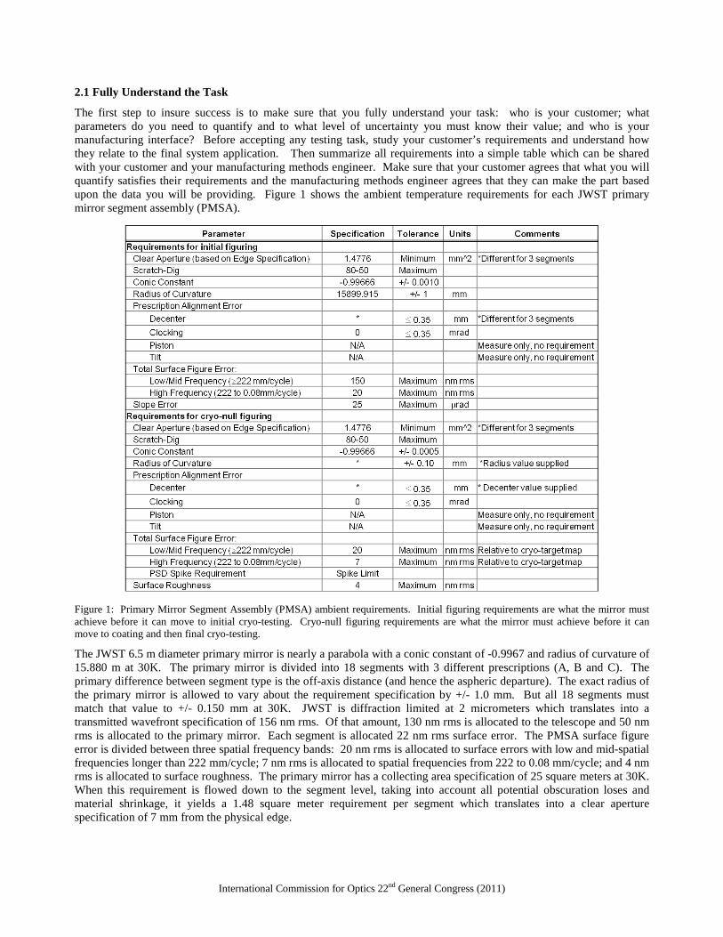
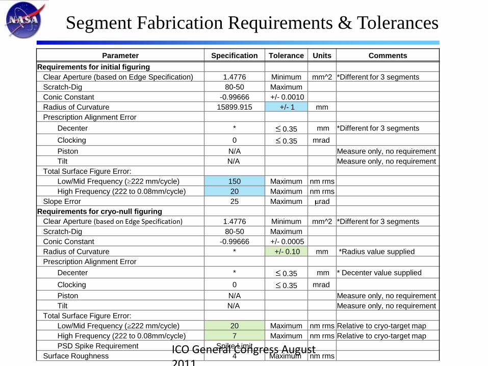
The first step to insure success is to make sure that you fully understand your task: who is your customer; what parameters do you need to quantify and to what level of uncertainty you must know their value; and who is your manufacturing interface? Before accepting any testing task, study your customer’s requirements and understand how they relate to the final system application. Then summarize all requirements into a simple table which can be shared with your customer and your manufacturing methods engineer. Make sure that your customer agrees that what you will quantify satisfies their requirements and the manufacturing methods engineer agrees that they can make the part based upon the data you will be providing. Figure 1 shows the ambient temperature requirements for each JWST primary mirror segment assembly (PMSA).

Figure 1: Primary Mirror Segment Assembly (PMSA) ambient requirements. Initial figuring requirements are what the mirror must achieve before it can move to initial cryo-testing. Cryo-null figuring requirements are what the mirror must achieve before it can move to coating and then final cryo-testing.

The JWST 6.5 m diameter primary mirror is nearly a parabola with a conic constant of -0.9967 and radius of curvature of 15.880 m at 30K. The primary mirror is divided into 18 segments with 3 different prescriptions (A, B and C). The primary difference between segment type is the off-axis distance (and hence the aspheric departure). The exact radius of the primary mirror is allowed to vary about the requirement specification by +/- 1.0 mm. But all 18 segments must match that value to +/- 0.150 mm at 30K. JWST is diffraction limited at 2 micrometers which translates into a transmitted wavefront specification of 156 nm rms. Of that amount, 130 nm rms is allocated to the telescope and 50 nm rms is allocated to the primary mirror. Each segment is allocated 22 nm rms surface error. The PMSA surface figure error is divided between three spatial frequency bands: 20 nm rms is allocated to surface errors with low and mid-spatial frequencies longer than 222 mm/cycle; 7 nm rms is allocated to spatial frequencies from 222 to 0.08 mm/cycle; and 4 nm rms is allocated to surface roughness. The primary mirror has a collecting area specification of 25 square meters at 30K. When this requirement is flowed down to the segment level, taking into account all potential obscuration loses and material shrinkage, it yields a 1.48 square meter requirement per segment which translates into a clear aperture specification of 7 mm from the physical edge.


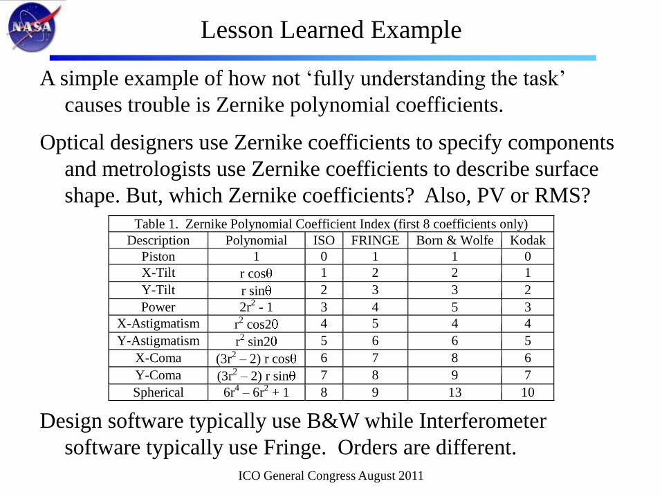
A simple example of how not following this rule causes trouble is Zernike polynomial coefficients. Many optical designers use Zernike coefficients to specify optical components and most optical metrologists use Zernike coefficients to describe surface shape – but, which Zernike coefficients. While there is an international standard for Zernike coefficient order (ISO 010110), no one seems to use it (Table 1). Most interferometer manufacturers use the University of Arizona FRINGE sequence (descended from ITEK). While many optical design programs use the University of Rochester Born & Wolfe sequence (descended from Zernike). And for some reason, Kodak had their own sequence. This problem is compounded because while most use Peak-to-Valley normalization (surface PV is 2X the coefficient value), some (such as the Perkin-Elmer) use RMS normalization. So, if the customer specifics that an optical component needs to have less than 10 nm of Z8, is that X-Coma (B&W), Y-Coma (Fringe), Spherical (ISO) or Trefoil (Kodak)?

Table 1. Zernike Polynomial Coefficient Index (first 8 coefficients only) Description Polynomial ISO FRINGE Born & Wolfe Kodak

Piston 1 0 1 1 0 X-Tilt r cosθ 1 2 2 1 Y-Tilt r sinθ 2 3 3 2 Power 2r2 3 - 1 4 5 3

X-Astigmatism r2 4 cos2θ 5 4 4 Y-Astigmatism r2 5 sin2θ 6 6 5

X-Coma (3r2 6 – 2) r cosθ 7 8 6 Y-Coma (3r2 7 – 2) r sinθ 8 9 7 Spherical 6r4 – 6r2 8 + 1 9 13 10

2.3 Develop an Error Budget

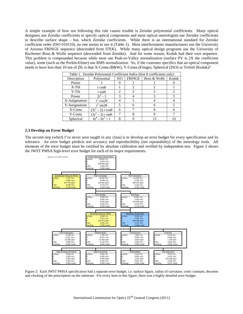
The second step (which I’ve never seen taught in any class) is to develop an error budget for every specification and its tolerance. An error budget predicts test accuracy and reproducibility (not repeatability) of the metrology tools. All elements of the error budget must be certified by absolute calibration and verified by independent test. Figure 2 shows the JWST PMSA high-level error budget for each of its major requirements.

Revision: 12-17-2007 13:49:25 Tinsley Fabrication Specificationsurface 20.000 nmR 0.100 mmK 500.000 ppmOAD 0.350 mmClocking 0.350 mrad

Specification Reserve (RSS) Part Knowledge Part Fabricationsurface 7.147 nm surface 12.025 nm surface 14.294 nmR 0.039 mm R 0.049 mm R 0.078 mmK 197.700 ppm K 233.609 ppm K 395.400 ppmOAD 0.095 mm OAD 0.279 mm OAD 0.190 mmClocking 0.146 mrad Clocking 0.128 mrad Clocking 0.291 mrad

Part Stability Metrologysurface 5.859 nm surface 10.501 nmR 0.042 mm R 0.026 mmK 0.000 ppm K 233.609 ppmOAD 0.002 mm OAD 0.279 mmClocking 0.000 mrad Clocking 0.128 mrad

Metrology Reserve (RSS) Metrology (Estimated)surface 4.696 nm surface 9.392 nmR 0.012 mm R 0.024 mmK 104.473 ppm K 208.946 ppmOAD 0.236 mm OAD 0.147 mmClocking 0.092 mrad Clocking 0.089 mrad

CGH Fabrication Interferometer Environment Fold Flatsurface 6.349 nm surface 1.293 nm surface 1.904 nm surface 6.519 nmR 0.010 mm R 0.017 mm R 0.000 mm R 0.005 mmK 35.956 ppm K 31.000 ppm K 0.000 ppm K 1.728 ppmOAD 0.009 mm OAD 0.116 mm OAD 0.000 mm OAD 0.000 mmClocking 0.005 mrad Clocking 0.046 mrad Clocking 0.000 mrad Clocking 0.000 mrad

Optical Design Residual Data Processing Repeatability Test Alignmentsurface 0.000 nm surface 0.000 nm surface 0.129 nm surface 0.319 nmR 0.000 mm R 0.000 mm R 0.001 mm R 0.012 mmK 0.000 ppm K 0.000 ppm K 2.531 ppm K 203.458 ppmOAD 0.000 mm OAD 0.000 mm OAD 0.001 mm OAD 0.090 mmClocking 0.000 mrad Clocking 0.000 mrad Clocking 0.000 mrad Clocking 0.075 mrad

Figure 2: Each JWST PMSA specification had a separate error budget, i.e. surface figure, radius of curvature, conic constant, decenter and clocking of the prescription on the substrate. For every item in this figure, there was a highly detailed error budget.


An error budget has multiple functions. First, it is necessary to convince your customer that you can actually measure the required parameters to the required tolerances. Second, it defines which test conditions have the greatest impact on test uncertainty. And third, it provides a tool for monitoring the test process. If the variability in the test data exceeds the error budget prediction, then you must stop and understand why.

The formal explanation of how to construct an error budget is to perform a propagation of error analysis. First write down the equation which calculates the specification value. Then take the partial derivative of that equation as a function of each variable. Square each result and multiple times the knowledge uncertainty (i.e. variance in data) for the measurement of each variable. Then take the square root of the sum. For example, assume that a requirement R is a function of variables (a,b,c), i.e. R = f(a, b, c). The uncertainty of the knowledge of the requirement R is give by:

If the defining equation is a linear sum, then the result is a simple root mean square of the individual standard deviations. But, if the equation is not linear, then there will be cross terms and scaling factors. In calculating standard deviations use reproducibility and not repeatability. Repeatability will give an ‘optimistic’ result. Reproducibility gives a realistic result. Repeatability is the ability to get the same answer twice if nothing in the test setup is changed. Reproducibility is the ability to get the same answer twice if the mirror is completely removed from and reinstalled into the test setup. From a real-world perspective, reproducibility is much more important than repeatability. For example, on JWST PMSAs are not only moved back and forth between manufacturing and test at Tinsley, but also from Tinsley to Ball Aerospace Technology Corporation (BATC) and the Marshall Space Flight Center (MSFC) X-Ray & Cryogenic Test Facility (XRCF). On JWST, a complete understanding of each metrology tool’s test uncertainty is critical. Data from Tinsley, BATC and the MSFC XRCF must reproduce each other within the test uncertainty. Certified cryo-data must be traceable from the XRCF where they are tested on their flight mount at 30K to BATC where they are changed from the flight mount to the fabrication mount at 300K to Tinsley where they are polished on their fabrication mount at 300K.

Finally, a personal lesson learned is not to wait too long to validate your error budget. On the ITTT program (which became Spitzer) I was the secondary mirror responsible metrology engineer. I had a complete error budget, but some elements were allocations. The secondary mirror was manufactured to a Hindle sphere test and the optician achieved an excellent result. Unfortunately, I didn’t calibrate the Hindle sphere until it was time to perform the final certification and, to my horror, it had a trefoil mount distortion. And, because the secondary mirror had a three point mount, every time it was inserted into the test, the bumps introduced by the optician exactly matched the holes in the Hindle sphere. Fortunately, the mirror still met its figure specification; it just was no long spectacular. The moral of the story is to not only validate your error budget early. But also, as much as possible, randomize your alignment from test to test. Sometimes bad things happen from been too meticulous. (This could almost be an 8th

2.3 Continuous Metrology Coverage

rule.)

The old adage (and its corollary) is correct: ‘you cannot make what you cannot test’ (or ‘if you can test it then you can make it’). The key to implementing these rules is simple. Every step of the manufacturing process must have metrology feedback and there must be overlap between the metrology tools for a verifiable transition. Failure to implement this rule typically results in one of two outcomes, either very slow convergence or negative convergence.

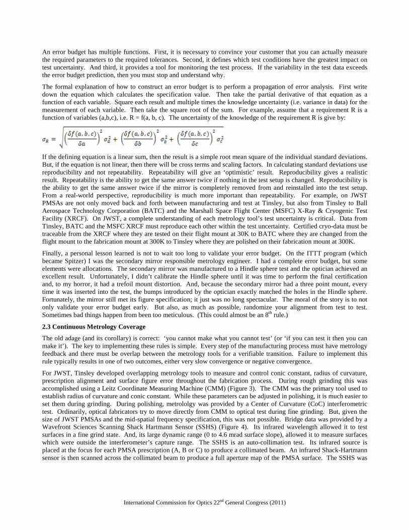
For JWST, Tinsley developed overlapping metrology tools to measure and control conic constant, radius of curvature, prescription alignment and surface figure error throughout the fabrication process. During rough grinding this was accomplished using a Leitz Coordinate Measuring Machine (CMM) (Figure 3). The CMM was the primary tool used to establish radius of curvature and conic constant. While these parameters can be adjusted in polishing, it is much easier to set them during grinding. During polishing, metrololgy was provided by a Center of Curvature (CoC) interferometric test. Ordinarily, optical fabricators try to move directly from CMM to optical test during fine grinding. But, given the size of JWST PMSAs and the mid-spatial frequency specification, this was not possible. Bridge data was provided by a Wavefront Sciences Scanning Shack Hartmann Sensor (SSHS) (Figure 4). Its infrared wavelength allowed it to test surfaces in a fine grind state. And, its large dynamic range (0 to 4.6 mrad surface slope), allowed it to measure surfaces which were outside the interferometer’s capture range. The SSHS is an auto-collimation test. Its infrared source is placed at the focus for each PMSA prescription (A, B or C) to produce a collimated beam. An infrared Shack-Hartmann sensor is then scanned across the collimated beam to produce a full aperture map of the PMSA surface. The SSHS was


only certified to provide mid-spatial frequency data from 222 to 2 mm. When not used, convergence was degraded. Figure 5 shows an example of the excellent data agreement between the CMM and SSHS.

Figure 3: Leitz Coordinate Measuring Machine (CMM) was used at Tinsley during generation and rough polishing to control radius of curvature, conic constant and aspheric figure for Primary Mirror Segment Assemblies, Secondary Mirrors and Tertiary Mirror.

Figure 4: Scanning Shack Hartmann Sensor (manufactured by Wavefront Sciences) is an auto-collimation test. A 10 micrometer source is placed at focus and a Shack-Hartmann sensor is scanned across the collimated beam. There are three different source positions for the three PMSA off-axis distances. Photo on right shows the sensor (white) mounted on the Paragon Gantry (black).

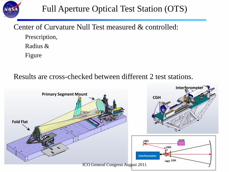
For fine grinding and polishing, metrology feedback is typically provided by interferometry. For JWST, this feedback was provided by a custom built optical test station (OTS) (Figure 6). The OTS is a multi-purpose test station combining the infrared SSHS, a center of curvature (CoC) interferometric test with a computer generated hologram (CGH) and an interferometric auto-collimation test. This test simultaneously controls conic constant, radius of curvature, prescription alignment and surface figure error. The CoC test pallet contains a 4D PhaseCAM, a Diffraction International CGH on a rotary mount and a Leica ADM. The ADM places the test pallet at the PMSA radius of curvature with an uncertainty of 0.100 mm which meets the radius knowledge requirement. Please note that this uncertainty is an error budget built up of many contributing factors. Once in this position, if the PMSA were perfect, its surface would exactly match the wavefront produced by the CGH. Any deviation from this null is a surface figure error to be corrected.

Figure 5: Comparison of CMM and SSHS data (for 222 to 2 mm spatial frequencies) after smooth out grind of the EDU (8/1/2006)

Figure 6: Optical Test Station (OTS) is a multi-purpose test setup with three different metrology tools: Scanning Shack Hartman Sensor, Center of Curvature CGH Interferometer and Auto-Collimation Interferometer.

Center of Curvature Test performed with interferometer and CGH at PMSA CoC

Autocollimation Test performed with IR source or interferometer at

PMSA focus(shown in two positions)

PMSA& Mount

IR SSHS Sensor scans collimated

beam using Paragon Gantry

Fold mirror is realigned for interferometric

auto-collimation test


2.4 Know Where You Are

It might seem simple, but if you don’t know where a feature is located on the mirror, you cannot correct it. To solve this problem you must use fiducials. There are two types of fiducials: Data Fiducials and Distortion Fiducials. Data fiducials are used to define a coordinate system and locate the measured data in that coordinate system. Sometimes this coordinate system is required to subtract calibration files, other times it is required to produce hit maps. Distortion fiducials are used to map out pupil distortion in the test setup. Many test setups, particularly those with null optics can have radial as well as lateral pupil distortion. Distortion can cause tool mis-registration errors of 10 to 50 mm or more.

Fiducials can be as simple as a piece of tape or black ink marks on the surface under test or as sophisticated as mechanical ‘fingers’ attached to the edge protruding into the clear aperture. While I have used tape fiducials for simple reproducibility or difference tests or to register a calibration alignment, I do not recommend them for computer controlled process metrology. In these cases, fiducials define your coordinate system and need to be applied with a mechanical precision of greater accuracy than the required prescription alignment to the substrate. Additionally, because the interferometer imaging system might invert the image or because fold mirrors in the test setup might introduce lateral flips, I highly recommend an asymmetric pattern. The pattern which I have always used is fiducials at 0, 30 (or 120), 90, and 180 degrees. The 0/180 degree fiducials produce a central axis for the data set. The 90 degree fiducial defines left/right and the 30 degree fiducial defines top/bottom. Additionally, for test setups with null optics, pupil distortion can be a problem. In these cases, distortion fiducials are required. One option is to place multiple fiducial marks along a radius. For null tests with anamorphic distortion, a grid of fiducial marks is recommended. Finally, if you have a clear aperture requirement, make sure to place fiducial marks inside and outside of the required clear aperture distance, this way you can certify whether or not the requirement is achieved.

Another problem is software coordinate convention. Most interferometer analysis software assumes that the optical (Z axis) positive direction points from the surface under test towards the interferometer, such that a feature which is higher than desired is positive. But, many optical design programs define the positive optical axis to be into the surface. The problem occurs because both programs will typically define the Y-axis as being up, so it is critical to understand which direction is +X-axis. (I have actually seen a software program which used a left handed coordinate system – talk about confusing.) The problem is further complicated when interfacing with the optical shop. A good metrologist needs to know the coordinate system of every computer controlled grinding and polishing machine. Every optical metrologist I know, including myself, has a story of the optical shop doubling the height or depth of a bump or hole because of a sign error, or adding a hole or bump to a surface because of a flip or inversion.

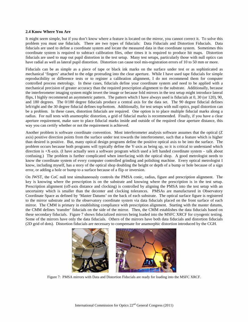
On JWST, the CoC null test simultaneously controls the PMSA conic, radius, figure and prescription alignment. The key is knowing where the prescription is on the substrate and knowing where the prescription is in the test setup. Prescription alignment (off-axis distance and clocking) is controlled by aligning the PMSA into the test setup with an uncertainty which is smaller than the decenter and clocking tolerances. PMSAs are manufactured in Observatory Coordinate Space as defined by ‘Master Datums’ on the back of each substrate. The optical surface figure is registered to the mirror substrate and to the observatory coordinate system via data fiducials placed on the front surface of each mirror. The CMM is primary in establishing compliance with prescription alignment. Starting with the master datums, the CMM defines ‘transfer’ fiducials on the side of the mirror. Then, the CMM establishes the data fiducials based on these secondary fiducials. Figure 7 shows fiducialized mirrors being loaded into the MSFC XRCF for cryogenic testing. Some of the mirrors have only the data fiducials. Others of the mirrors have both data fiducials and distortion fiducials (2D grid of dots). Distortion fiducials are necessary to compensate for anamorphic distortion introduced by the CGH.

Figure 7: PMSA mirrors with Data and Distortion Fiducials are ready for loading into the MSFC XRCF.


2.5 Test like you Fly

‘Test like you fly’ covers a wide range of situations. For example, JWST operates in the cold of space. Therefore, it is necessary to certify not only its 30K optical performance, but also its ‘zero-g’ performance. Spitzer mirrors had to be certified at 4K. But this rule is not limited to space telescopes. Large ground based telescopes can have large gravity sags. Therefore, they must be tested in their final structure (or a suitable surrogate) at an operational gravity orientation. Gravity is not typically a problem for small, stiff mirrors. But, it can be a significant problem for large mirrors. Another problem is non-kinematic mounts. Once I had a task to test an ‘egg-crate’ 0.75 meter diameter flat mirror to 30 nm PV. After some initial characterization tests with the customer, I declined. The customer provided ‘metrology’ mount was unsuitable. The mirror was so ‘floppy’ (i.e. low stiffness) that simply picking it up and setting it back down onto the metrology mount resulted in a 100 nm PV shape change (both astigmatic bending and local mount induced stress).

Because JWST mirrors are fabricated at room temperature (300K) but will operate in the cold of space (< 50K), it is necessary to measure their shape change from 300 K to 30K, generate a ‘hit-map’, and cryo-null polish the mirrors such that they satisfy their required figure specification at 30K. After coating, all mirrors undergo a final cryo-certification test of conic constant, radius of curvature, prescription alignment and surface figure error (low/mid and part of high) is accomplished at 30K in the MSFC XRCF and cross-checked at 30K in the JSC Chamber A. But, clear aperture, high spatial frequency figure error and surface roughness are certified at Ambient with the Tinsley High Spatial and Surface Roughness Test Station and confirmed as best as possible at XRCF. In these cases, it is assumed that the parameter’s measured properties are independent of temperature.

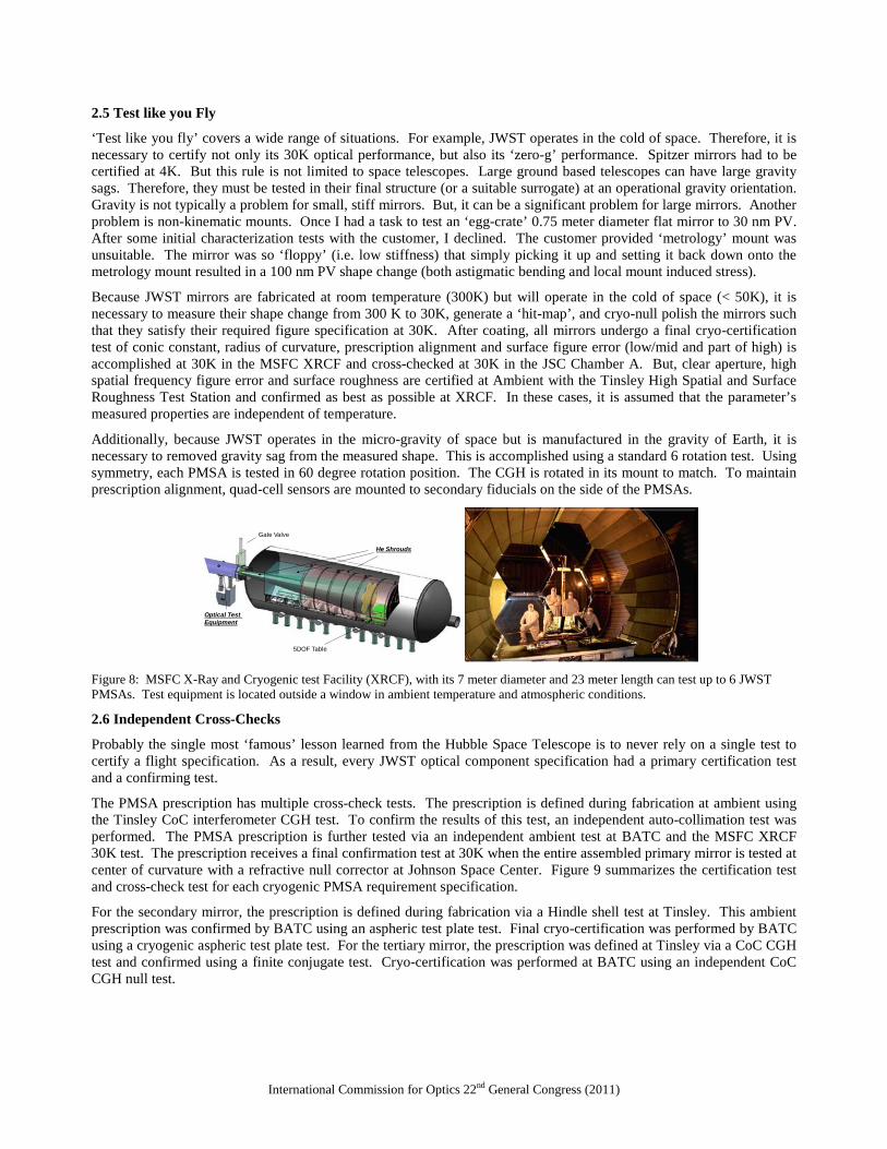
Additionally, because JWST operates in the micro-gravity of space but is manufactured in the gravity of Earth, it is necessary to removed gravity sag from the measured shape. This is accomplished using a standard 6 rotation test. Using symmetry, each PMSA is tested in 60 degree rotation position. The CGH is rotated in its mount to match. To maintain prescription alignment, quad-cell sensors are mounted to secondary fiducials on the side of the PMSAs.

He Shrouds

Gate Valve

Optical Test Equipment

5DOF Table

Figure 8: MSFC X-Ray and Cryogenic test Facility (XRCF), with its 7 meter diameter and 23 meter length can test up to 6 JWST PMSAs. Test equipment is located outside a window in ambient temperature and atmospheric conditions.

2.6 Independent Cross-Checks

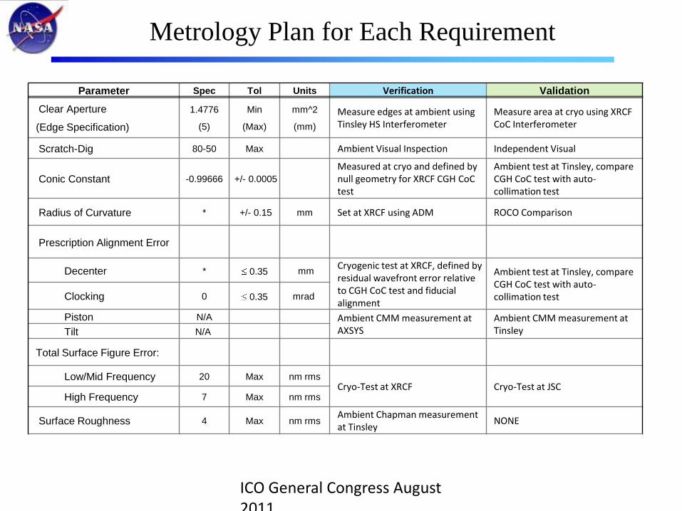
Probably the single most ‘famous’ lesson learned from the Hubble Space Telescope is to never rely on a single test to certify a flight specification. As a result, every JWST optical component specification had a primary certification test and a confirming test.

The PMSA prescription has multiple cross-check tests. The prescription is defined during fabrication at ambient using the Tinsley CoC interferometer CGH test. To confirm the results of this test, an independent auto-collimation test was performed. The PMSA prescription is further tested via an independent ambient test at BATC and the MSFC XRCF 30K test. The prescription receives a final confirmation test at 30K when the entire assembled primary mirror is tested at center of curvature with a refractive null corrector at Johnson Space Center. Figure 9 summarizes the certification test and cross-check test for each cryogenic PMSA requirement specification.

For the secondary mirror, the prescription is defined during fabrication via a Hindle shell test at Tinsley. This ambient prescription was confirmed by BATC using an aspheric test plate test. Final cryo-certification was performed by BATC using a cryogenic aspheric test plate test. For the tertiary mirror, the prescription was defined at Tinsley via a CoC CGH test and confirmed using a finite conjugate test. Cryo-certification was performed at BATC using an independent CoC CGH null test.


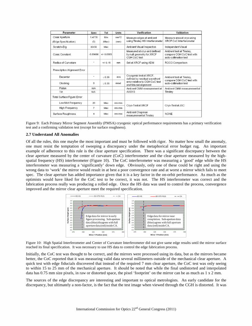
Figure 9: Each Primary Mirror Segment Assembly (PMSA) cryogenic optical performance requirements has a primary verification test and a confirming validation test (except for surface roughness).

2.7 Understand All Anomalies

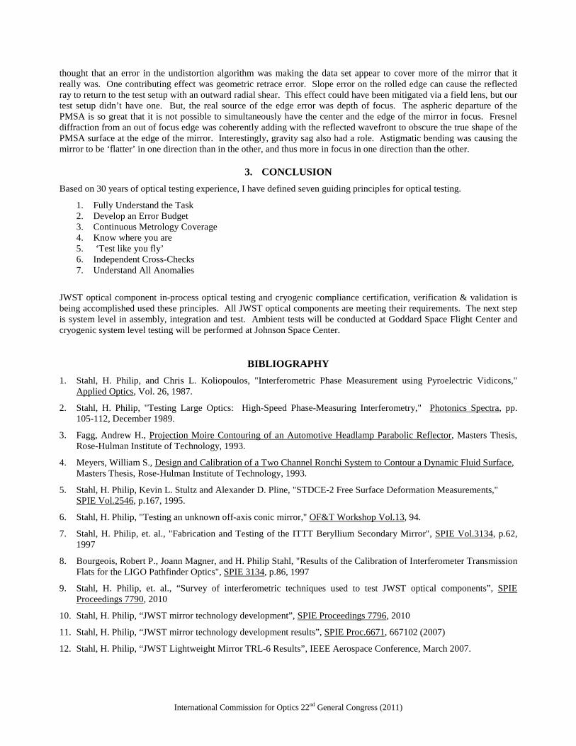
Of all the rules, this one maybe the most important and must be followed with rigor. No matter how small the anomaly, one must resist the temptation of sweeping a discrepancy under the metaphorical error budget rug. An important example of adherence to this rule is the clear aperture specification. There was a significant discrepancy between the clear aperture measured by the center of curvature (CoC) interferometer and the clear aperture measured by the high-spatial frequency (HS) interferometer (Figure 10). The CoC interferometer was measuring a ‘good’ edge while the HS interferometer was measuring a ‘significantly’ down edge. Obviously, only one of these could be right and using the wrong data to ‘work’ the mirror would result in at best a poor convergence rate and at worst a mirror which fails to meet spec. The clear aperture has added importance given that it is a key factor in the on-orbit performance. As much as the optimists would have liked for the CoC test to be correct, it was not. The HS interferometer was correct and the fabrication process really was producing a rolled edge. Once the HS data was used to control the process, convergence improved and the mirror clear aperture meet the required specification.

-5.0

-4.5

-4.0-3.5

-3.0

-2.5

-2.0

-1.5

-1.0-0.5

0.0

0.5

1.0

-675 -650 -625 -600 -575 -550

Miiror Y-Position (mm)

Surfa

ce H

eigh

t (µm

)

B3 HS B3 OTS R121 CA

-5.0

-4.5

-4.0-3.5

-3.0

-2.5

-2.0

-1.5

-1.0-0.5

0.0

0.5

1.0

-675 -650 -625 -600 -575 -550


Surf

ace

Heig

ht (µ

m)


Edge data for mirror in early figure processing. Sub-aperture data (blue) disagrees with full aperture data (red) inside CA.

Edge data for mirror near completion. Sub-aperture data (blue) agrees with full aperture data (red) inside CA.

Figure 10: High Spatial Interferometer and Center of Curvature Interferometer did not give same edge results until the mirror surface reached its final specification. It was necessary to use HS data to control the edge fabrication process.

Initially, the CoC test was thought to be correct, and the mirrors were processed using its data, but as the mirrors became better, the CoC reported that it was measuring valid data several millimeters outside of the mechanical clear aperture. A quick test with edge fiducials discovered that instead of the required 7 mm clear aperture, the CoC test was only seeing to within 15 to 25 mm of the mechanical aperture. It should be noted that while the final undistorted and interpolated data has 0.75 mm size pixels, in raw or distorted space, the pixel ‘footprint’ on the mirror can be as much as 1 x 2 mm.

The sources of the edge discrepancy are interesting and important to optical metrologists. An early candidate for the discrepancy, but ultimately a non-factor, is the fact that the test image when viewed through the CGH is distorted. It was


thought that an error in the undistortion algorithm was making the data set appear to cover more of the mirror that it really was. One contributing effect was geometric retrace error. Slope error on the rolled edge can cause the reflected ray to return to the test setup with an outward radial shear. This effect could have been mitigated via a field lens, but our test setup didn’t have one. But, the real source of the edge error was depth of focus. The aspheric departure of the PMSA is so great that it is not possible to simultaneously have the center and the edge of the mirror in focus. Fresnel diffraction from an out of focus edge was coherently adding with the reflected wavefront to obscure the true shape of the PMSA surface at the edge of the mirror. Interestingly, gravity sag also had a role. Astigmatic bending was causing the mirror to be ‘flatter’ in one direction than in the other, and thus more in focus in one direction than the other.

3. CONCLUSION Based on 30 years of optical testing experience, I have defined seven guiding principles for optical testing.

1. Fully Understand the Task 2. Develop an Error Budget 3. Continuous Metrology Coverage 4. Know where you are 5. ‘Test like you fly’ 6. Independent Cross-Checks 7. Understand All Anomalies

JWST optical component in-process optical testing and cryogenic compliance certification, verification & validation is being accomplished used these principles. All JWST optical components are meeting their requirements. The next step is system level in assembly, integration and test. Ambient tests will be conducted at Goddard Space Flight Center and cryogenic system level testing will be performed at Johnson Space Center.

BIBLIOGRAPHY

1. Stahl, H. Philip, and Chris L. Koliopoulos, "Interferometric Phase Measurement using Pyroelectric Vidicons," Applied Optics

2. Stahl, H. Philip, "Testing Large Optics: High-Speed Phase-Measuring Interferometry,"

, Vol. 26, 1987.

Photonics Spectra

3. Fagg, Andrew H.,

, pp. 105-112, December 1989.

Projection Moire Contouring of an Automotive Headlamp Parabolic Reflector

4. Meyers, William S.,

, Masters Thesis, Rose-Hulman Institute of Technology, 1993.

Design and Calibration of a Two Channel Ronchi System to Contour a Dynamic Fluid Surface

5. Stahl, H. Philip, Kevin L. Stultz and Alexander D. Pline, "STDCE-2 Free Surface Deformation Measurements,"

, Masters Thesis, Rose-Hulman Institute of Technology, 1993.

SPIE Vol.2546

6. Stahl, H. Philip, "Testing an unknown off-axis conic mirror,"

, p.167, 1995.

OF&T Workshop Vol.13

7. Stahl, H. Philip, et. al., "Fabrication and Testing of the ITTT Beryllium Secondary Mirror",

, 94.

SPIE Vol.3134

8. Bourgeois, Robert P., Joann Magner, and H. Philip Stahl, "Results of the Calibration of Interferometer Transmission Flats for the LIGO Pathfinder Optics",

, p.62, 1997

SPIE 3134

9. Stahl, H. Philip, et. al., “Survey of interferometric techniques used to test JWST optical components”,

, p.86, 1997

SPIE Proceedings 7790

10. Stahl, H. Philip, “JWST mirror technology development”,

, 2010

SPIE Proceedings 7796

11. Stahl, H. Philip, “JWST mirror technology development results”,

, 2010

SPIE Proc.6671

12. Stahl, H. Philip, “JWST Lightweight Mirror TRL-6 Results”, IEEE Aerospace Conference, March 2007.

, 667102 (2007)


H. Philip Stahl, PhD

NASA Marshall Space Flight Center, Huntsville, AL

ICO General Congress August 2011


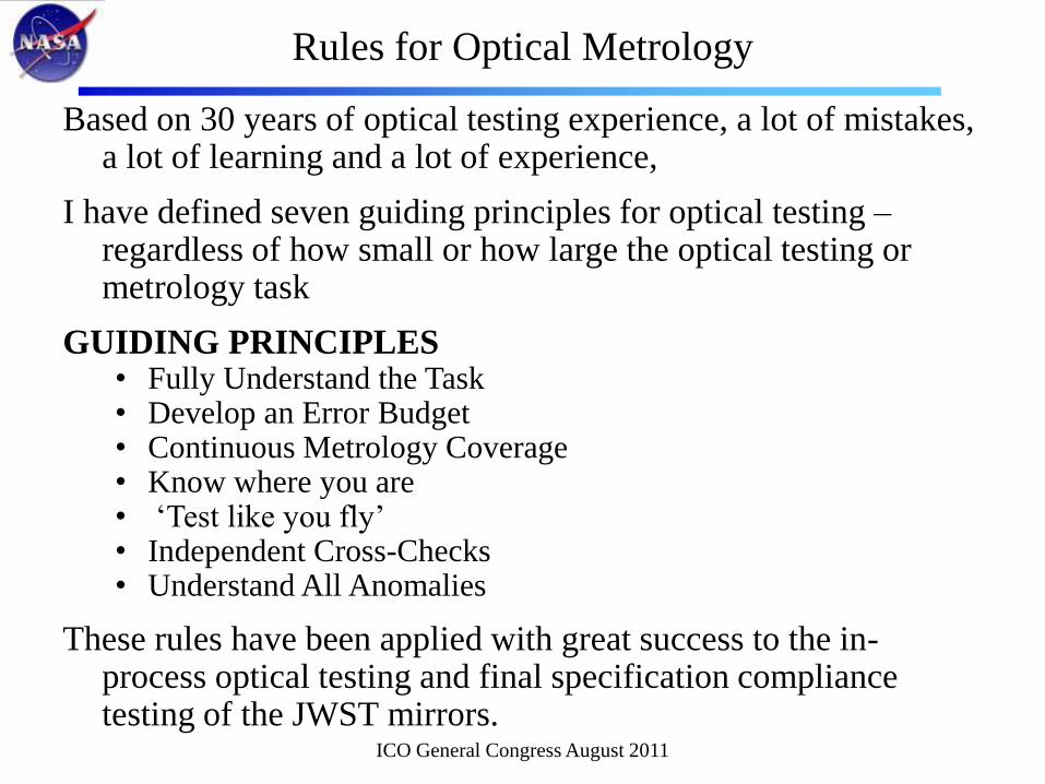
Based on 30 years of optical testing experience, a lot of mistakes, a lot of learning and a lot of experience,

I have defined seven guiding principles for optical testing –regardless of how small or how large the optical testing or metrology task

GUIDING PRINCIPLES• Fully Understand the Task• Develop an Error Budget• Continuous Metrology Coverage• Know where you are• ‘Test like you fly’ • Independent Cross-Checks• Understand All Anomalies

These rules have been applied with great success to the in-process optical testing and final specification compliance testing of the JWST mirrors.


Fully Understand the Task

First, make sure that you fully understand your task: who is your customer;

what parameters do you need to quantify;

to what level of uncertainty you must know their value; and

who is your manufacturing interface?

Before accepting any testing task, study your customer’s requirements and understand how they relate to the final system application.

Then summarize all requirements into a simple table which can be shared with your customer and your manufacturing methods engineer.

Make sure that your customer agrees that what you will quantify satisfies their requirements and the manufacturing methods engineer agrees that they can make the part based upon the data you will be providing.


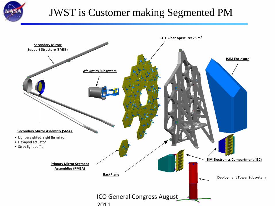
JWST is Customer making Segmented PM

Secondary Mirror Support Structure (SMSS)

Primary Mirror SegmentAssemblies (PMSA)

BackPlane

OTE Clear Aperture: 25 m2

ISIM Enclosure

Aft Optics Subsystem

Secondary Mirror Assembly (SMA)

• Light-weighted, rigid Be mirror• Hexapod actuator• Stray light baffle

Deployment Tower Subsystem

ISIM Electronics Compartment (IEC)


Segment Fabrication Requirements & Tolerances

Parameter Specification Tolerance Units CommentsRequirements for initial figuring

Clear Aperture (based on Edge Specification) 1.4776 Minimum mm^2 *Different for 3 segmentsScratch-Dig 80-50 MaximumConic Constant -0.99666 +/- 0.0010Radius of Curvature 15899.915 +/- 1 mmPrescription Alignment Error

Decenter * 0.35 mm *Different for 3 segmentsClocking 0 0.35 mradPiston N/A Measure only, no requirementTilt N/A Measure only, no requirement

Total Surface Figure Error:Low/Mid Frequency ( 222 mm/cycle) 150 Maximum nm rmsHigh Frequency (222 to 0.08mm/cycle) 20 Maximum nm rms

Slope Error 25 Maximum radRequirements for cryo-null figuring

Clear Aperture (based on Edge Specification) 1.4776 Minimum mm^2 *Different for 3 segmentsScratch-Dig 80-50 MaximumConic Constant -0.99666 +/- 0.0005Radius of Curvature * +/- 0.10 mm *Radius value suppliedPrescription Alignment Error

Decenter * 0.35 mm * Decenter value suppliedClocking 0 0.35 mradPiston N/A Measure only, no requirementTilt N/A Measure only, no requirement

Total Surface Figure Error:Low/Mid Frequency ( 222 mm/cycle) 20 Maximum nm rms Relative to cryo-target mapHigh Frequency (222 to 0.08mm/cycle) 7 Maximum nm rms Relative to cryo-target mapPSD Spike Requirement Spike Limit

Surface Roughness 4 Maximum nm rmsICO General Congress August 2011

Metrology Plan for Each Requirement

Parameter Spec Tol Units Verification Validation

Clear Aperture

(Edge Specification)

1.4776

(5)

Min

(Max)

mm^2

(mm)Measure edges at ambient using Tinsley HS Interferometer

Measure area at cryo using XRCF CoC Interferometer

Scratch-Dig 80-50 Max Ambient Visual Inspection Independent Visual

Conic Constant -0.99666 +/- 0.0005Measured at cryo and defined by null geometry for XRCF CGH CoCtest

Ambient test at Tinsley, compare CGH CoC test with auto-collimation test

Radius of Curvature * +/- 0.15 mm Set at XRCF using ADM ROCO Comparison

Prescription Alignment Error

Decenter * 0.35 mm Cryogenic test at XRCF, defined by residual wavefront error relative to CGH CoC test and fiducialalignment

Ambient test at Tinsley, compare CGH CoC test with auto-collimation testClocking 0 0.35 mrad

Piston N/A Ambient CMM measurement at AXSYS

Ambient CMM measurement at TinsleyTilt N/A

Total Surface Figure Error:

Low/Mid Frequency 20 Max nm rmsCryo-Test at XRCF Cryo-Test at JSC

High Frequency 7 Max nm rms

Surface Roughness 4 Max nm rms Ambient Chapman measurement at Tinsley

NONE


Lesson Learned Example

A simple example of how not ‘fully understanding the task’

causes trouble is Zernike polynomial coefficients.

Optical designers use Zernike coefficients to specify components

and metrologists use Zernike coefficients to describe surface

shape. But, which Zernike coefficients? Also, PV or RMS?

Design software typically use B&W while Interferometer

software typically use Fringe. Orders are different.

Table 1. Zernike Polynomial Coefficient Index (first 8 coefficients only)

Description Polynomial ISO FRINGE Born & Wolfe Kodak

Piston 1 0 1 1 0

X-Tilt r cos 1 2 2 1

Y-Tilt r sin 2 3 3 2

Power 2r2 - 1 3 4 5 3

X-Astigmatism r2 cos2 4 5 4 4

Y-Astigmatism r2 sin2 5 6 6 5

X-Coma (3r2 – 2) r cos 6 7 8 6

Y-Coma (3r2 – 2) r sin 7 8 9 7

Spherical 6r4 – 6r2 + 1 8 9 13 10


Develop an Error Budget

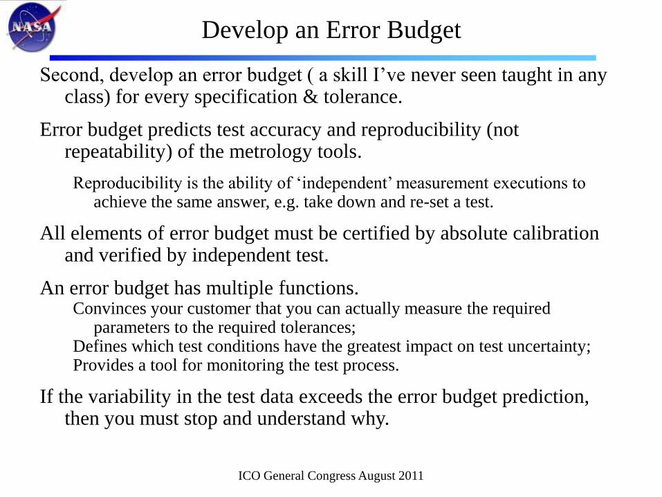
Second, develop an error budget ( a skill I’ve never seen taught in any class) for every specification & tolerance.

Error budget predicts test accuracy and reproducibility (not repeatability) of the metrology tools.

Reproducibility is the ability of ‘independent’ measurement executions to achieve the same answer, e.g. take down and re-set a test.

All elements of error budget must be certified by absolute calibration and verified by independent test.

An error budget has multiple functions. Convinces your customer that you can actually measure the required

parameters to the required tolerances; Defines which test conditions have the greatest impact on test uncertainty; Provides a tool for monitoring the test process.

If the variability in the test data exceeds the error budget prediction, then you must stop and understand why.


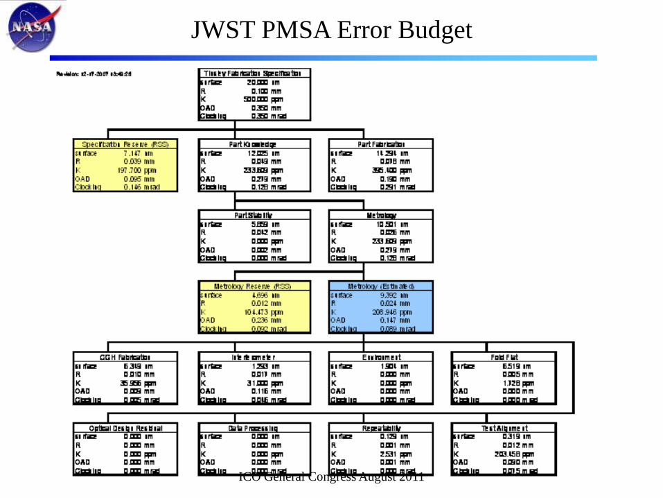
JWST PMSA Error Budget


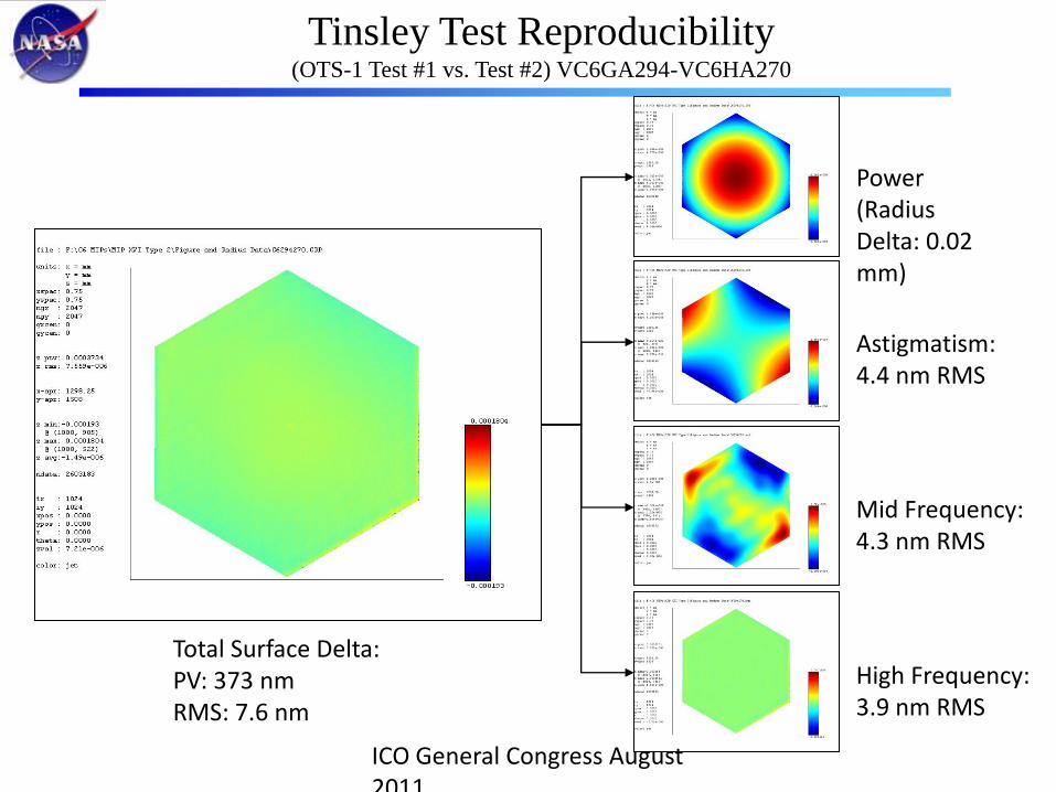
Tinsley Test Reproducibility(OTS-1 Test #1 vs. Test #2) VC6GA294-VC6HA270

Power(Radius Delta: 0.02 mm)

Astigmatism:4.4 nm RMS

Mid Frequency:4.3 nm RMS

High Frequency:3.9 nm RMS

Total Surface Delta:PV: 373 nmRMS: 7.6 nm


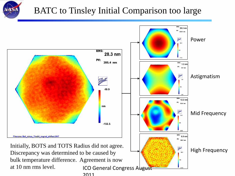
BATC to Tinsley Initial Comparison too large

Astigmatism

Mid Frequency

High Frequency

Power

Initially, BOTS and TOTS Radius did not agree.

Discrepancy was determined to be caused by

bulk temperature difference. Agreement is now

at 10 nm rms level. ICO General Congress August 2011

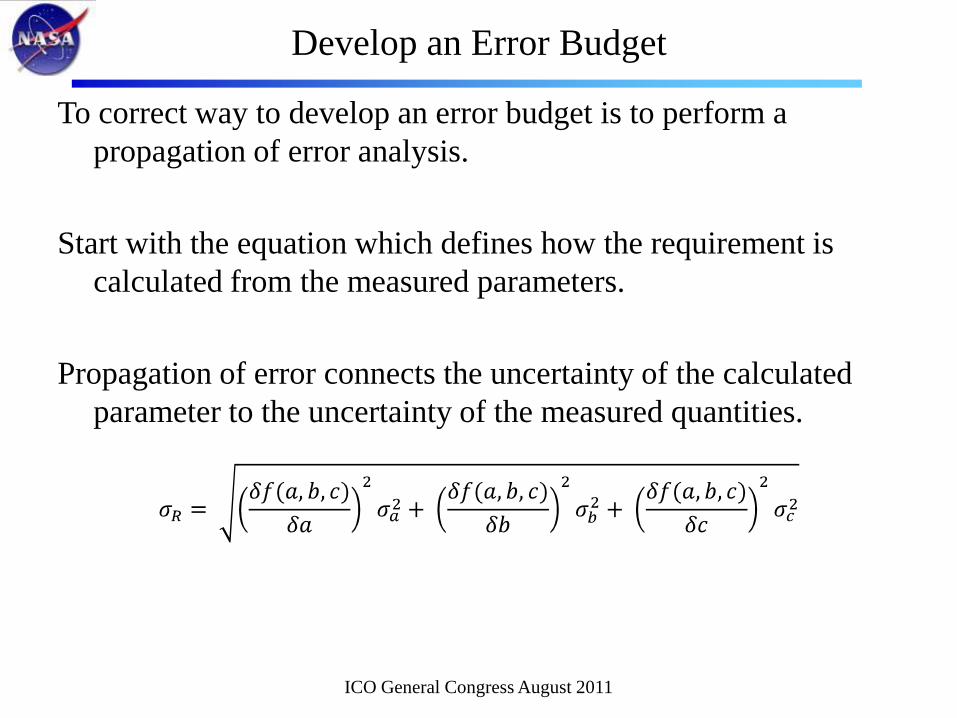
Develop an Error Budget

To correct way to develop an error budget is to perform a

propagation of error analysis.

Start with the equation which defines how the requirement is

calculated from the measured parameters.

Propagation of error connects the uncertainty of the calculated

parameter to the uncertainty of the measured quantities.


Lesson Learned – validate error budget early

On ITTT program (which became Spitzer) I was SM engineer.

I had a complete error budget, but some elements were allocations.

Secondary Mirror was manufactured to a Hindle sphere test and the optician achieved an excellent result.

Unfortunately, I didn’t calibrate the Hindle sphere until it was time to perform the final certification and it had a trefoil mount distortion.

Because SM had a three point mount, every time it was tested, the bumps on the SM exactly matched the holes in the Hindle sphere.

Fortunately, it still met specification; it was just not spectacular.

Moral of the story:Validate your error budget early, andAs much as possible, randomize your alignment from test to test.

Sometimes bad things happen from been too meticulous. (This could almost be an 8th rule.)


Continuous Metrology Coverage

Third, have continuous metrology coverage:

‘you cannot make what you cannot test’

(or ‘if you can test it then you can make it’).

Every step of the manufacturing process must have metrology

feedback and there must be overlap between the metrology

tools for a verifiable transition.

Failure to implement this rule typically results in one of two

outcomes:

very slow convergence, or

negative convergence.



JWST developed overlapping tools to measure & control

conic constant,

radius of curvature,

prescription alignment and surface figure error

throughout the fabrication process.

During rough grinding, used a Leitz Coordinate Measuring

Machine (CMM) for radius of curvature & conic constant.

During polishing, meterololgy was provided by a Center of

Curvature (CoC) interferometric test.


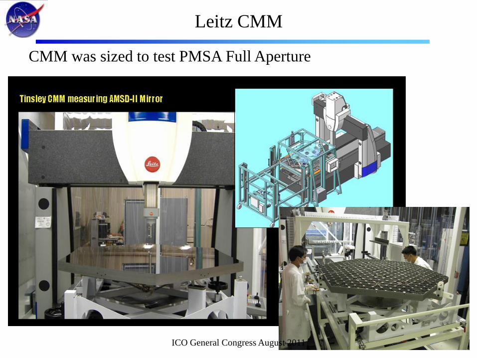
CMM was sized to test PMSA Full Aperture

Leitz CMM


CGH

Interferometer

Fold Flat

Primary Segment Mount

Full Aperture Optical Test Station (OTS)

Center of Curvature Null Test measured & controlled:

Prescription,

Radius &

Figure

Results are cross-checked between different 2 test stations.

ADM

CGH

Interferometer

M2

M3

M1



Ordinarily, optical fabricators try to move directly from CMM to

optical test during fine grinding. But, given the size of JWST

PMSAs and the mid-spatial frequency specification, this was

not possible.

Bridge data was provided by a Wavefront Sciences Scanning

Shack Hartmann Sensor (SSHS).

Its infrared wavelength allowed it to test surfaces in a fine grind state.

And, its large dynamic range (0 to 4.6 mrad surface slope), allowed it to

measure surfaces which were outside the interferometer’s capture

range.


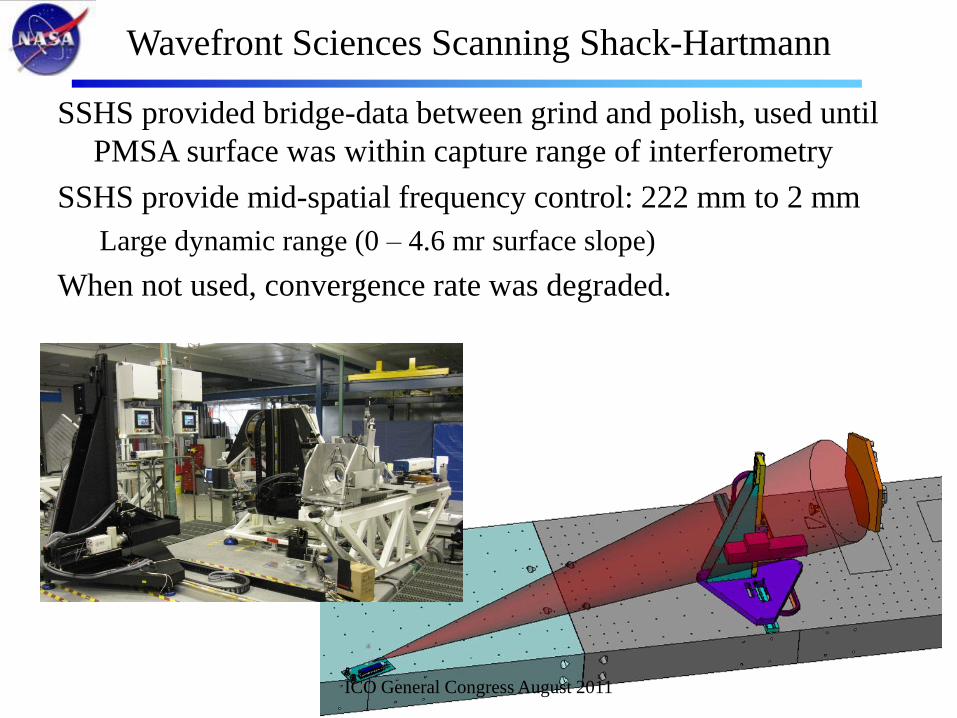
SSHS provided bridge-data between grind and polish, used until

PMSA surface was within capture range of interferometry

SSHS provide mid-spatial frequency control: 222 mm to 2 mm

Large dynamic range (0 – 4.6 mr surface slope)

When not used, convergence rate was degraded.

Wavefront Sciences Scanning Shack-Hartmann


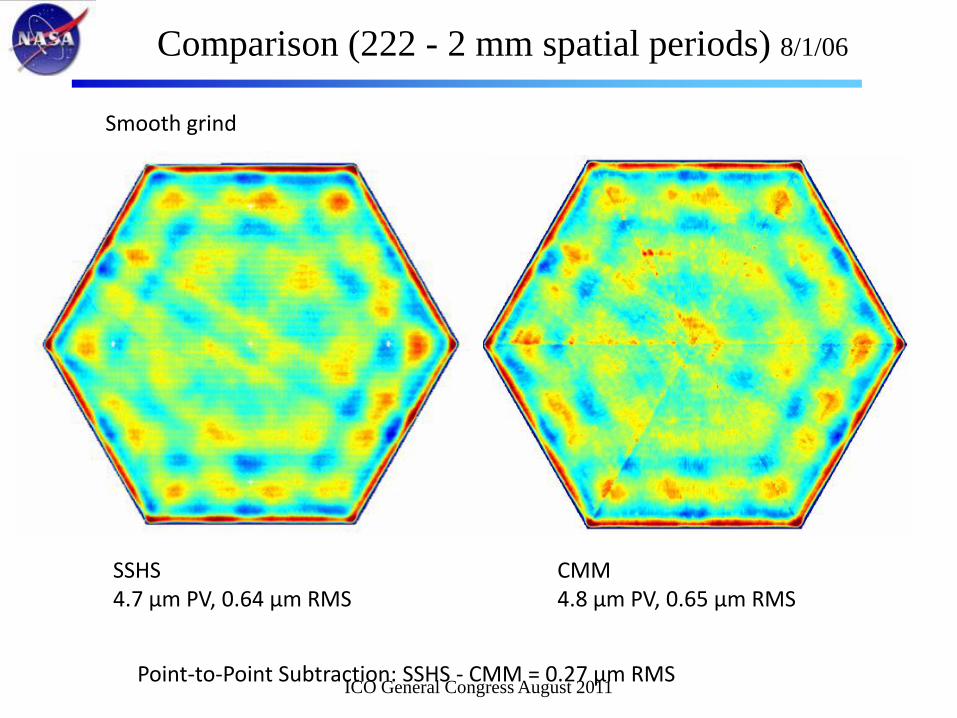
Comparison (222 - 2 mm spatial periods) 8/1/06

SSHS4.7 µm PV, 0.64 µm RMS

CMM4.8 µm PV, 0.65 µm RMS

Smooth grind

Point-to-Point Subtraction: SSHS - CMM = 0.27 µm RMSICO General Congress August 2011

Know where you are

Fourth, know where you are. It might seem simple, but if you don’t know where a feature is located on the mirror, you cannot correct it. This requires fiducials.

There are two types of fiducials: Data Fiducials and Distortion Fiducials.

Data fiducials are used to define a coordinate system and locate the measured data in that coordinate system. Sometimes this coordinate system is required to subtract calibration files, other times it is required to produce hit maps.

Distortion fiducials are used to map out test setup pupil distortion. Many test setups, particularly those with null optics can have radial as well as lateral pupil distortion. Distortion can cause tool mis-registration errors of 10 to 50 mm or more.


Fiducials

Fiducials can be as simple as a piece of tape or ink marks on surface under test or as sophisticated as mechanical ‘fingers’ protruding into clear aperture.

For computer controlled processes, fiducial positional knowledge is critical.

Because test setups might invert or flip the imaging, I highly recommend an asymmetric pattern. The pattern which I have always used is:

0/180 degree fiducials produce a central axis for the data set,

90 degree fiducial defines left/right, and

30 degree fiducial defines top/bottom.

For rotationally symmetric systems, one option for distortion fiducials is multiple marks along a radius.

But for asymmetric systems, a grid of marks is required.

Finally, if you have a clear aperture requirement, place marks inside and outside of the required clear aperture.


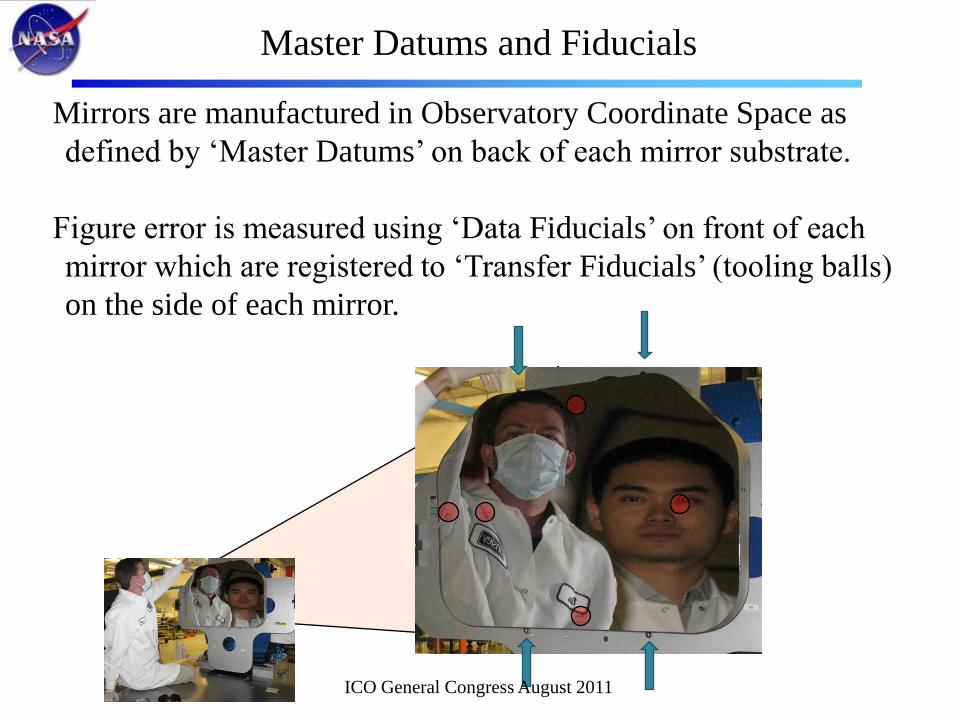
Mirrors are manufactured in Observatory Coordinate Space as

defined by ‘Master Datums’ on back of each mirror substrate.

Figure error is measured using ‘Data Fiducials’ on front of each

mirror which are registered to ‘Transfer Fiducials’ (tooling balls)

on the side of each mirror.

Master Datums and Fiducials


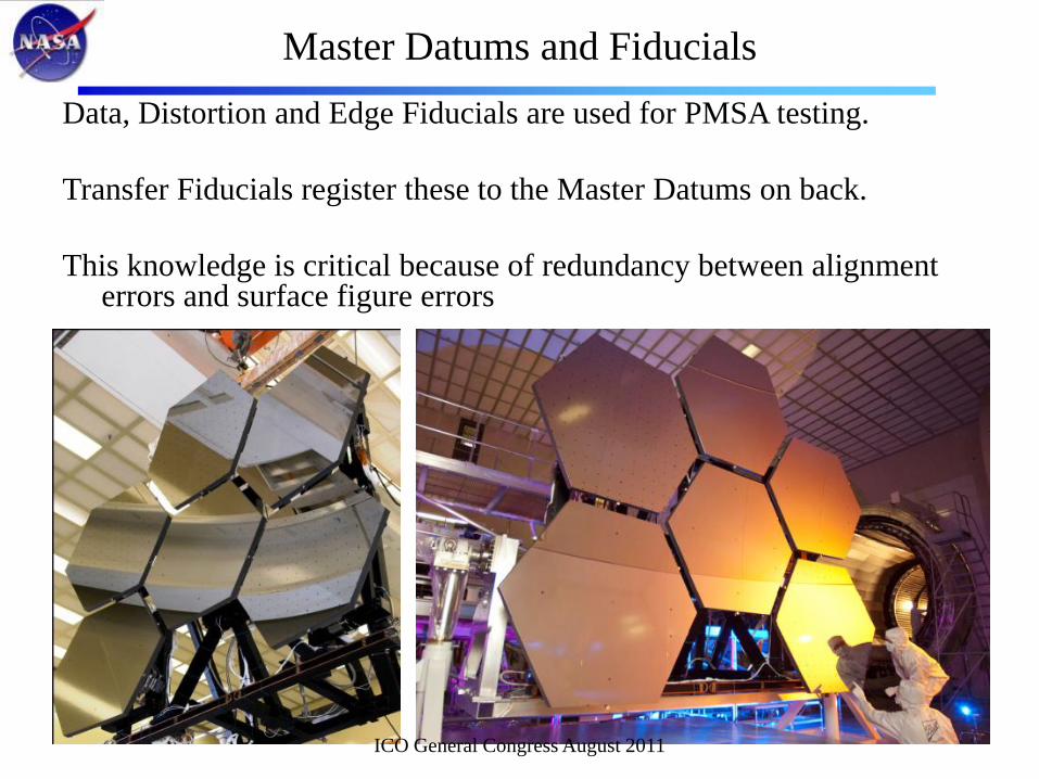
Master Datums and Fiducials

Data, Distortion and Edge Fiducials are used for PMSA testing.

Transfer Fiducials register these to the Master Datums on back.

This knowledge is critical because of redundancy between alignment errors and surface figure errors


Lesson Learned

Another problem is software coordinate convention.

Most interferometer analysis software assumes that the optical (Z

axis) positive direction points from the surface under test

towards the interferometer, such that a feature which is higher

than desired is positive.

But, many optical design programs define the positive optical

axis to be into the surface.

The problem occurs because both programs will typically define

the Y-axis as being up, so it is critical to understand which

direction is +X-axis. (I have actually seen a software program

which used a left handed coordinate system)

The problem is further complicated when interfacing with the

optical shop. You must know the coordinate system of every

computer controlled grinding and polishing machine.


‘Test like you fly’

Fifth, you must ‘Test like you fly’.

JWST operates in the cold of space. Therefore, we must certify

30K optical performance in the MSFC XRCF, and

‘zero-g’ performance via a 6 rotation test at BATC BOTS.

Observatory level qualification < 50K is done at JSC Chamber A.

Also, ‘test as you fly’ is not limited to space telescopes. Ground

based telescopes can have large gravity sags.

Therefore, they must be tested in their final structure (or a surrogate).


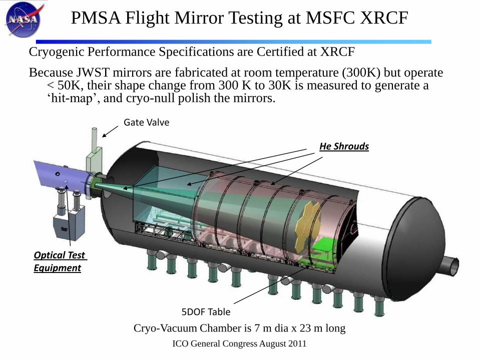
He Shrouds

Gate Valve

Optical Test Equipment

5DOF Table

Cryogenic Performance Specifications are Certified at XRCF

Because JWST mirrors are fabricated at room temperature (300K) but operate < 50K, their shape change from 300 K to 30K is measured to generate a ‘hit-map’, and cryo-null polish the mirrors.

Cryo-Vacuum Chamber is 7 m dia x 23 m long

PMSA Flight Mirror Testing at MSFC XRCF


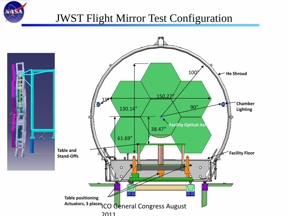
JWST Flight Mirror Test Configuration

15”

61.69”

38.47”

100”

150.27”

130.14” 90”

Facility Optical Axis

He Shroud

Facility FloorTable and Stand-Offs

Table positioning Actuators, 3 places

Chamber Lighting


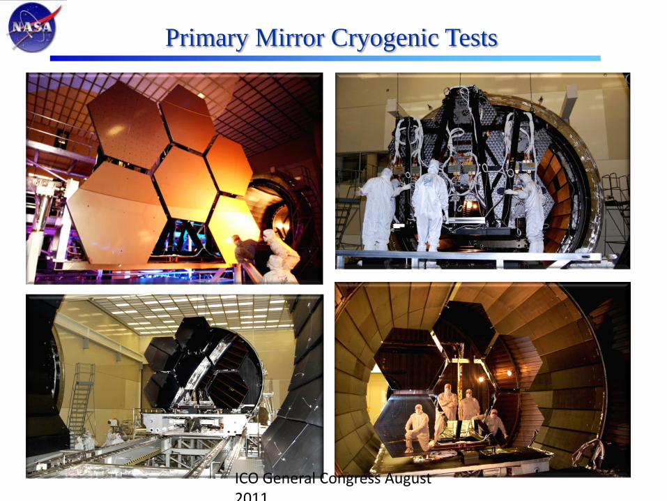
Primary Mirror Cryogenic Tests


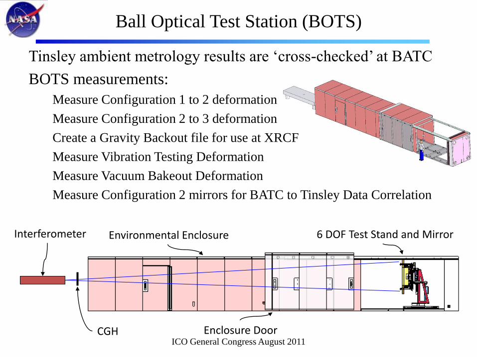
Ball Optical Test Station (BOTS)

Tinsley ambient metrology results are ‘cross-checked’ at BATC

BOTS measurements:

Measure Configuration 1 to 2 deformation

Measure Configuration 2 to 3 deformation

Create a Gravity Backout file for use at XRCF

Measure Vibration Testing Deformation

Measure Vacuum Bakeout Deformation

Measure Configuration 2 mirrors for BATC to Tinsley Data Correlation

Interferometer

CGH

Environmental Enclosure

Enclosure Door

6 DOF Test Stand and Mirror


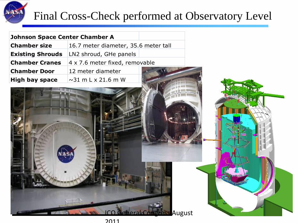
Final Cross-Check performed at Observatory Level

Johnson Space Center Chamber A

Chamber size 16.7 meter diameter, 35.6 meter tall

Existing Shrouds LN2 shroud, GHe panels

Chamber Cranes 4 x 7.6 meter fixed, removable

Chamber Door 12 meter diameter

High bay space ~31 m L x 21.6 m W


Lesson Learned

While Gravity is a significant problem for large mirrors.

It is also problem for lightweight mirrors in non-kinematic

mounts

Once I had a task to test an ‘egg-crate’ 0.75 meter diameter flat

mirror to 30 nm PV.

After initial characterization tests with the customer, I declined.

The customer provided ‘metrology’ mount was unsuitable.

The mirror was so ‘floppy’ (i.e. low stiffness) that simply picking

it up and setting it back down onto the metrology mount

resulted in a 100 nm PV shape change (both astigmatic

bending and local mount stress).


Independent Cross-Checks

Sixth, Independent Cross-Checks.

Probably the single most ‘famous’ lesson learned from Hubble is

to never rely on a single test to certify a flight specification.

Every JWST optical component specification had a primary

certification test and a confirming test.


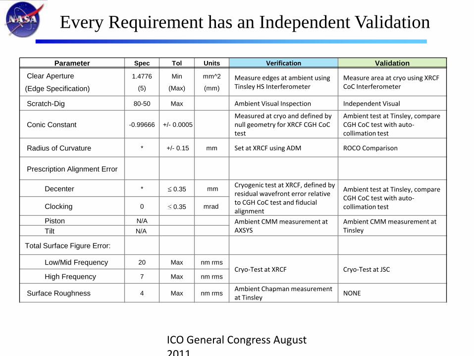
Every Requirement has an Independent Validation

Parameter Spec Tol Units Verification Validation

Clear Aperture

(Edge Specification)

1.4776

(5)

Min

(Max)

mm^2

(mm)Measure edges at ambient using Tinsley HS Interferometer

Measure area at cryo using XRCF CoC Interferometer

Scratch-Dig 80-50 Max Ambient Visual Inspection Independent Visual

Conic Constant -0.99666 +/- 0.0005Measured at cryo and defined by null geometry for XRCF CGH CoCtest

Ambient test at Tinsley, compare CGH CoC test with auto-collimation test

Radius of Curvature * +/- 0.15 mm Set at XRCF using ADM ROCO Comparison

Prescription Alignment Error

Decenter * 0.35 mm Cryogenic test at XRCF, defined by residual wavefront error relative to CGH CoC test and fiducialalignment

Ambient test at Tinsley, compare CGH CoC test with auto-collimation testClocking 0 0.35 mrad

Piston N/A Ambient CMM measurement at AXSYS

Ambient CMM measurement at TinsleyTilt N/A

Total Surface Figure Error:

Low/Mid Frequency 20 Max nm rmsCryo-Test at XRCF Cryo-Test at JSC

High Frequency 7 Max nm rms

Surface Roughness 4 Max nm rms Ambient Chapman measurement at Tinsley

NONE


Understand All Anomalies

Finally, understand all anomalies.

Of all the rules, this one maybe the most important and must be

followed with independent rigor.

No matter how small, one must resist the temptation of sweeping

a discrepancy under the metaphorical error budget rug.


Lesson Learned: Clear Aperture Edge Specification

-5.0

-4.5

-4.0-3.5

-3.0

-2.5

-2.0

-1.5

-1.0-0.5

0.0

0.5

1.0

-675 -650 -625 -600 -575 -550


Surfa

ce H

eigh

t (µm

)


-5.0

-4.5

-4.0

-3.5

-3.0

-2.5-2.0

-1.5

-1.0

-0.5

0.0

0.5

1.0

550 575 600 625 650 675


Surfa

ce H

eigh

t (µm

)


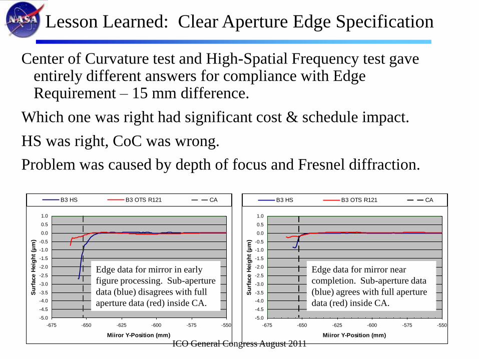
Center of Curvature test and High-Spatial Frequency test gave entirely different answers for compliance with Edge Requirement – 15 mm difference.

Which one was right had significant cost & schedule impact.

HS was right, CoC was wrong.

Problem was caused by depth of focus and Fresnel diffraction.

-5.0

-4.5

-4.0-3.5

-3.0

-2.5

-2.0

-1.5

-1.0-0.5

0.0

0.5

1.0

-675 -650 -625 -600 -575 -550


Surfa

ce H

eigh

t (µm

)


-5.0

-4.5

-4.0

-3.5

-3.0

-2.5-2.0

-1.5

-1.0

-0.5

0.0

0.5

1.0

550 575 600 625 650 675


Surfa

ce H

eigh

t (µm

)


Edge data for mirror in early

figure processing. Sub-aperture

data (blue) disagrees with full

aperture data (red) inside CA.

Edge data for mirror near

completion. Sub-aperture data

(blue) agrees with full aperture

data (red) inside CA.


Conclusions

Based on 30 years of optical testing experience, I have defined seven guiding principles for optical testing. • Fully Understand the Task

• Develop an Error Budget

• Continuous Metrology Coverage

• Know where you are

• ‘Test like you fly’

• Independent Cross-Checks

• Understand All Anomalies

With maybe an 8th of deliberately disturbing or randomizing the test.

JWST optical component in-process optical testing and cryogenic compliance certification, verification & validation was accomplished by a dedicated metrology team used these principles.

All JWST optical components meet their requirements.


Rules for Optical Metrology - NASA · PDF fileRules for Optical Metrology. H. Philip Stahl,...

Documents

Transcript of Rules for Optical Metrology - NASA · PDF fileRules for Optical Metrology. H. Philip Stahl,...