Rue La La - MIT presentation
32
Analytics for an Online Retailer: Demand Forecasting and Price Optimization Kris Johnson – MIT, Operations Research Center Alex Lee – MIT, Systems Design & Management Murali Narayanaswamy – Rue La La, VP Pricing & Operations Strategy Philip Roizin – Rue La La, Chief Financial Officer David Simchi-Levi – MIT, Operations Research Center Jonathan Waggoner – Rue La La, Chief Operating Officer
Transcript of Rue La La - MIT presentation
Analytics for an Online Retailer:
Demand Forecasting and Price Optimization
Kris Johnson – MIT, Operations Research Center
Alex Lee – MIT, Systems Design & Management
Murali Narayanaswamy – Rue La La, VP Pricing & Operations Strategy
Philip Roizin – Rue La La, Chief Financial Officer
David Simchi-Levi – MIT, Operations Research Center
Jonathan Waggoner – Rue La La, Chief Operating Officer
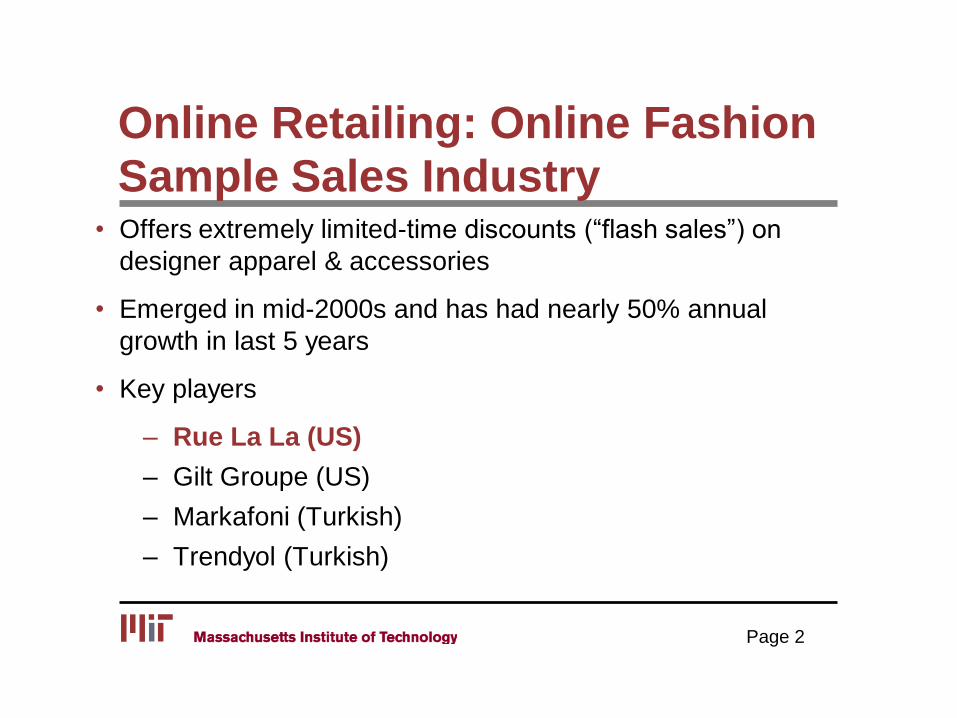
Online Retailing: Online Fashion
Sample Sales Industry • Offers extremely limited-time discounts (“flash sales”) on
designer apparel & accessories
• Emerged in mid-2000s and has had nearly 50% annual
growth in last 5 years
• Key players
– Rue La La (US)
– Gilt Groupe (US)
– Markafoni (Turkish)
– Trendyol (Turkish)
Page 2

Page 3
Snapshot of Rue La La’s Website

“Style”
Page 4

“SKU”
Page 5

Flash Sales Operations
Merchants
purchase items
from designers
Designers
ship items to
warehouse*
Merchants decide
when to sell items
(create “event”)
During event,
customers
purchase items
Sell out
of item?
End
*Sometimes designer will hold inventory
Yes
No
First event that style is
sold = “1st exposure”

https://www.youtube.com/watch?v=ahOHAsECeIw&feature=youtu.be

*Data disguised to protect confidentiality
0%
10%
20%
30%
40%
50%
60%
70%
0%-25% 25%-50% 50%-75% 75%-100% SOLD OUT(100%)
% o
f It
em
s
% Inventory Sold (Sell-Through)
1st Exposure Sell-Through Distribution
Department 1
Department 2
Department 3
Department 4
Department 5
Page 9
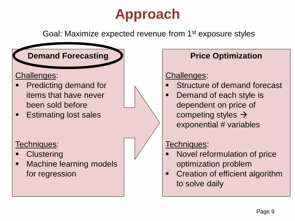
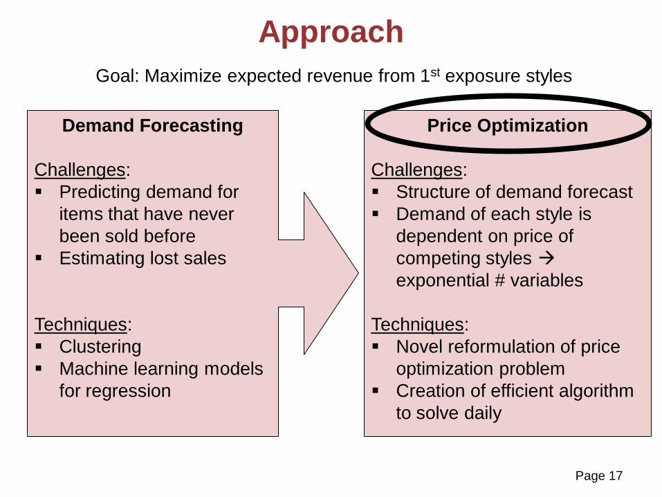
Approach
Goal: Maximize expected revenue from 1st exposure styles
Demand Forecasting
Challenges:
Predicting demand for
items that have never
been sold before
Estimating lost sales
Techniques:
Clustering
Machine learning models
for regression
Price Optimization
Challenges:
Structure of demand forecast
Demand of each style is
dependent on price of
competing styles
exponential # variables
Techniques:
Novel reformulation of price
optimization problem
Creation of efficient algorithm
to solve daily
Page 10
0%
10%
20%
30%
40%
50%
60%
70%
80%
90%
100%
0 1 2 3 4 5 6 7 8 9 10 11 12 13 14 15 16 17 18 19 20 21 22 23 24 25 26 27 28 29 30 31 32 33 34 35 36 37 38 39 40 41 42 43 44 45 46 47 48
Perc
en
t o
f To
tal
Sale
s
Hours Into Event
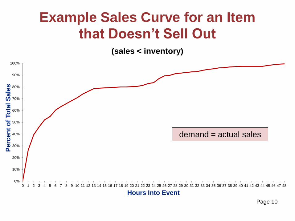
Example Sales Curve for an Item
that Doesn’t Sell Out (sales < inventory)
demand = actual sales

Page 11
0%
10%
20%
30%
40%
50%
60%
70%
80%
90%
100%
0 1 2 3 4 5 6 7 8 9 10 11 12 13 14 15 16 17 18 19 20 21 22 23 24 25 26 27 28 29 30 31 32 33 34 35 36 37 38 39 40 41 42 43 44 45 46 47 48
Perc
en
t o
f To
tal
Sale
s
Hours Into Event
Example Sales Curve for an Item
that Does Sell Out (sales = inventory)
demand = actual sales +
estimated lost sales during
period after stock out
stock out 10 hours into event
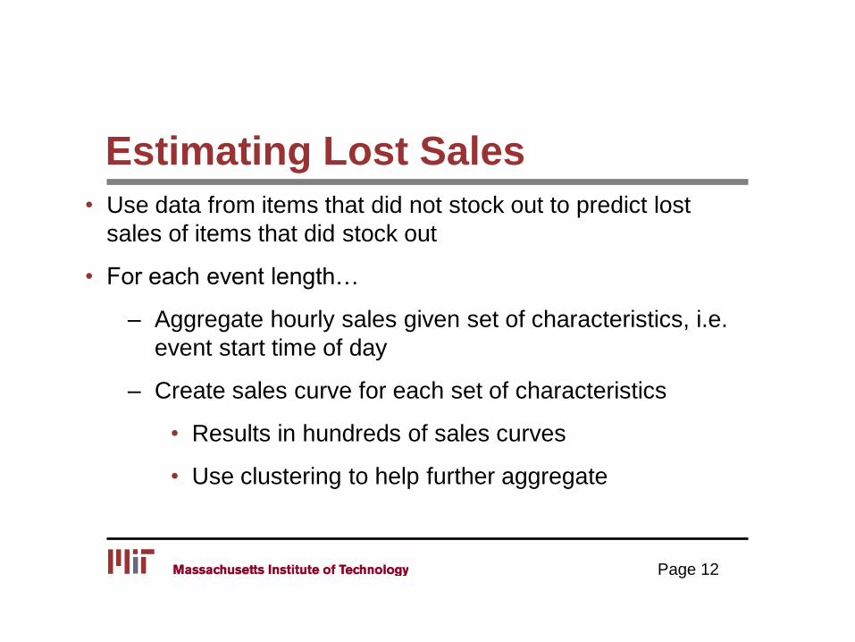
Estimating Lost Sales
• Use data from items that did not stock out to predict lost
sales of items that did stock out
• For each event length…
– Aggregate hourly sales given set of characteristics, i.e.
event start time of day
– Create sales curve for each set of characteristics
• Results in hundreds of sales curves
• Use clustering to help further aggregate
Page 12
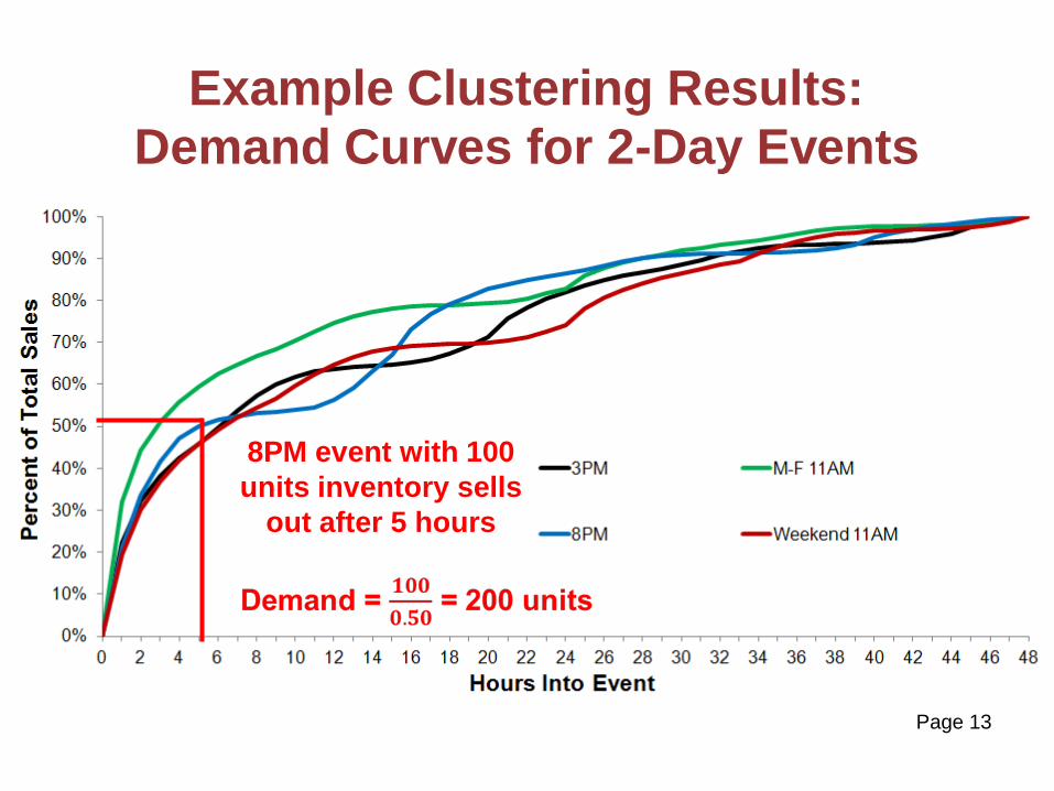
Page 13
Example Clustering Results:
Demand Curves for 2-Day Events
8PM event with 100
units inventory sells
out after 5 hours
Page 14
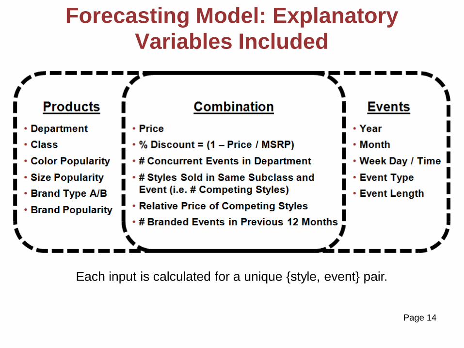
Forecasting Model: Explanatory
Variables Included
Each input is calculated for a unique {style, event} pair.
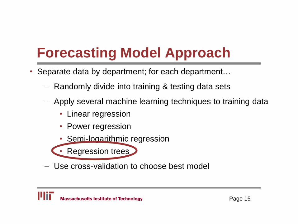
Forecasting Model Approach
• Separate data by department; for each department…
– Randomly divide into training & testing data sets
– Apply several machine learning techniques to training data
• Linear regression
• Power regression
• Semi-logarithmic regression
• Regression trees
– Use cross-validation to choose best model
Page 15
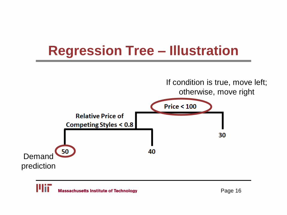
Regression Tree – Illustration
Page 16
If condition is true, move left;
otherwise, move right
Demand
prediction
Page 17
Approach
Goal: Maximize expected revenue from 1st exposure styles
Demand Forecasting
Challenges:
Predicting demand for
items that have never
been sold before
Estimating lost sales
Techniques:
Clustering
Machine learning models
for regression
Price Optimization
Challenges:
Structure of demand forecast
Demand of each style is
dependent on price of
competing styles
exponential # variables
Techniques:
Novel reformulation of price
optimization problem
Creation of efficient algorithm
to solve daily

Complexity
• Three of the features used to predict demand are associated
with pricing
– Price
– % Discount =
– Relative Price of Competing Styles =
• Pricing must be optimized concurrently for all
competing styles
Page 18
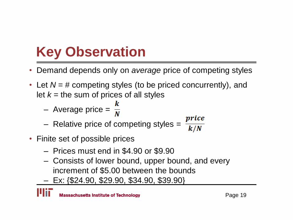
Key Observation
Page 19
• Demand depends only on average price of competing styles
• Let N = # competing styles (to be priced concurrently), and
let k = the sum of prices of all styles
– Average price =
– Relative price of competing styles =
• Finite set of possible prices
– Prices must end in $4.90 or $9.90
– Consists of lower bound, upper bound, and every
increment of $5.00 between the bounds
– Ex: {$24.90, $29.90, $34.90, $39.90}

Key Idea for Algorithm
• Formulate integer optimization problem for each value of k, (IPk)
Maximize Revenue
1) Each style must be assigned exactly one price
2) Sum of prices of all styles must = k
Page 20
s.t.
• Can show that optimal objective of (IPk) and its linear relaxation
only differ by the revenue associated with a single style!
– Independent of problem size
• Use this to develop efficient algorithm to solve on daily basis

IMPLEMENTATION & IMPACT
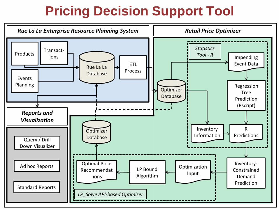
Pricing Decision Support Tool
ETL Process
Optimization Input
Optimal Price Recommendat
-ions
Rue La La Database
Reports and Visualization
Ad hoc Reports
Query / Drill Down Visualizer
Standard Reports
Optimizer Database
Optimizer Database
Rue La La Enterprise Resource Planning System
Products Transact-
ions
Statistics Tool - R
Events Planning
Inventory-Constrained
Demand Prediction
Regression Tree
Prediction (Rscript)
Impending Event Data
R Predictions
Inventory Information
Retail Price Optimizer
LP Bound Algorithm
LP_Solve API-based Optimizer

https://www.youtube.com/watch?v=lc4wV6O_YDA&feature=youtu.be
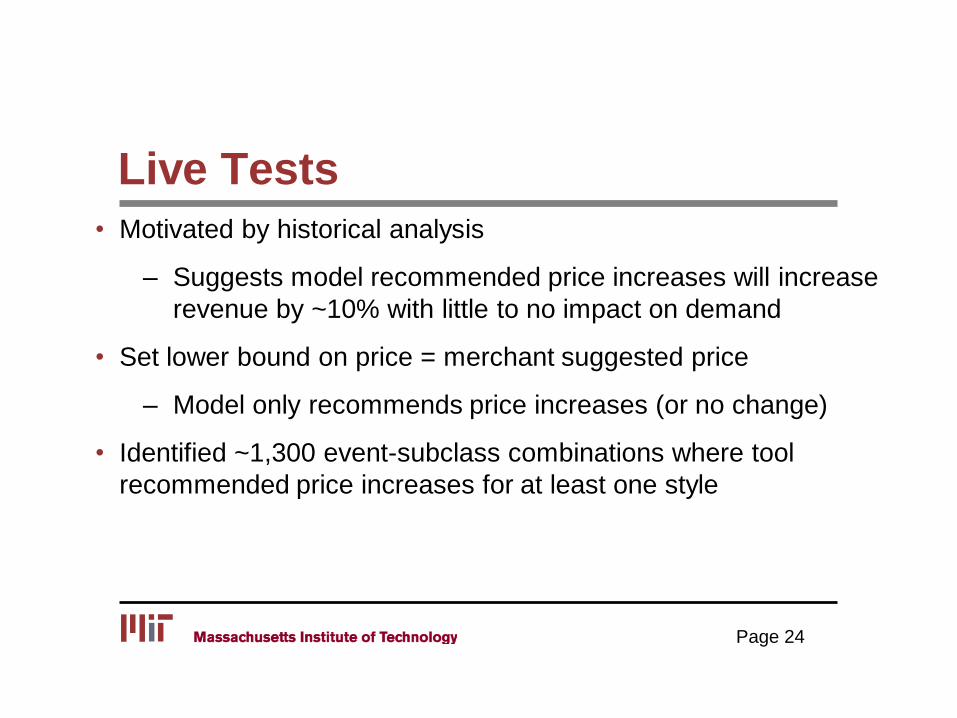
Live Tests
• Motivated by historical analysis
– Suggests model recommended price increases will increase
revenue by ~10% with little to no impact on demand
• Set lower bound on price = merchant suggested price
– Model only recommends price increases (or no change)
• Identified ~1,300 event-subclass combinations where tool
recommended price increases for at least one style
Page 24
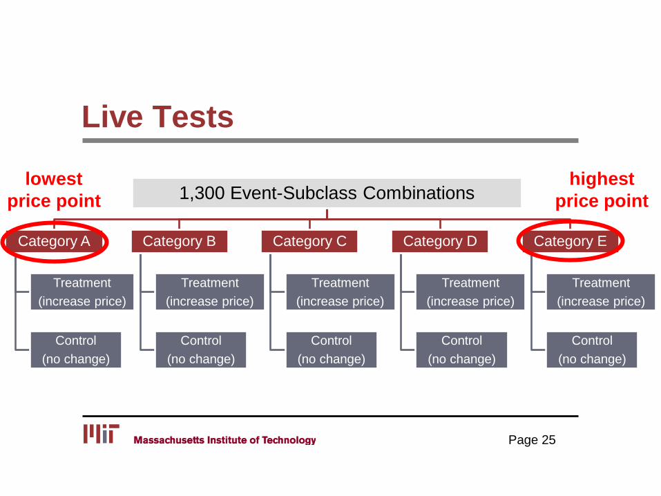
Live Tests
1,300 Event-Subclass Combinations
Category A
Treatment
(increase price)
Control
(no change)
Category B
Treatment
(increase price)
Control
(no change)
Category C
Treatment
(increase price)
Control
(no change)
Category D
Treatment
(increase price)
Control
(no change)
Category E
Treatment
(increase price)
Control
(no change)
lowest
price point
highest
price point
Page 25

Mann-Whitney /
Wilcoxon Rank Sum Test • Hypothesis test that assumes no particular distributional form
on treatment or control groups
– H0: raising prices has no effect on sell-through
– HA: raising prices decreases sell-through
• Idea of test
– Combine sell-through data of treatment and control groups
– Order data and assign rank to each observation
– Sum ranks of all treatment group observations
– If sum is too low, reject H0
Page 26

Mann-Whitney /
Wilcoxon Rank Sum Test
Page 27
1,300 Event-Subclass Combinations
Category A
Treatment
(increase price)
Control
(no change)
Category B
Treatment
(increase price)
Control
(no change)
Category C
Treatment
(increase price)
Control
(no change)
Category D
Treatment
(increase price)
Control
(no change)
Category E
Treatment
(increase price)
Control
(no change)
Rejects H0
α = 1%
Does not
reject H0
α = 10%
Does not
reject H0
α = 20%
Does not
reject H0
α = 20%
Does not
reject H0
α = 20%
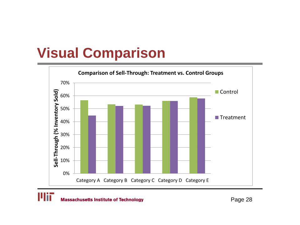
Visual Comparison
Page 28
0%
10%
20%
30%
40%
50%
60%
70%
Category A Category B Category C Category D Category E
Sell-
Thro
ugh
(%
Inve
nto
ry S
old
)
Comparison of Sell-Through: Treatment vs. Control Groups
Control
Treatment
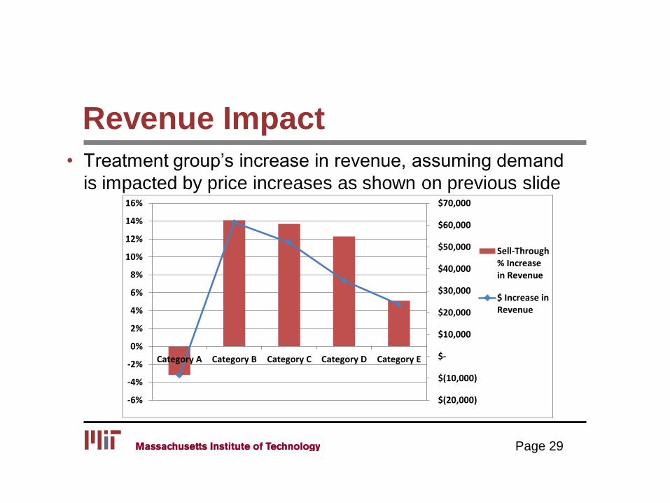
Revenue Impact
• Treatment group’s increase in revenue, assuming demand
is impacted by price increases as shown on previous slide
Page 29
$(20,000)
$(10,000)
$-
$10,000
$20,000
$30,000
$40,000
$50,000
$60,000
$70,000
-6%
-4%
-2%
0%
2%
4%
6%
8%
10%
12%
14%
16%
Category A Category B Category C Category D Category E
Sell-Through% Increasein Revenue
$ Increase inRevenue

https://www.youtube.com/watch?v=AzJhAxkpkEU&feature=youtu.be
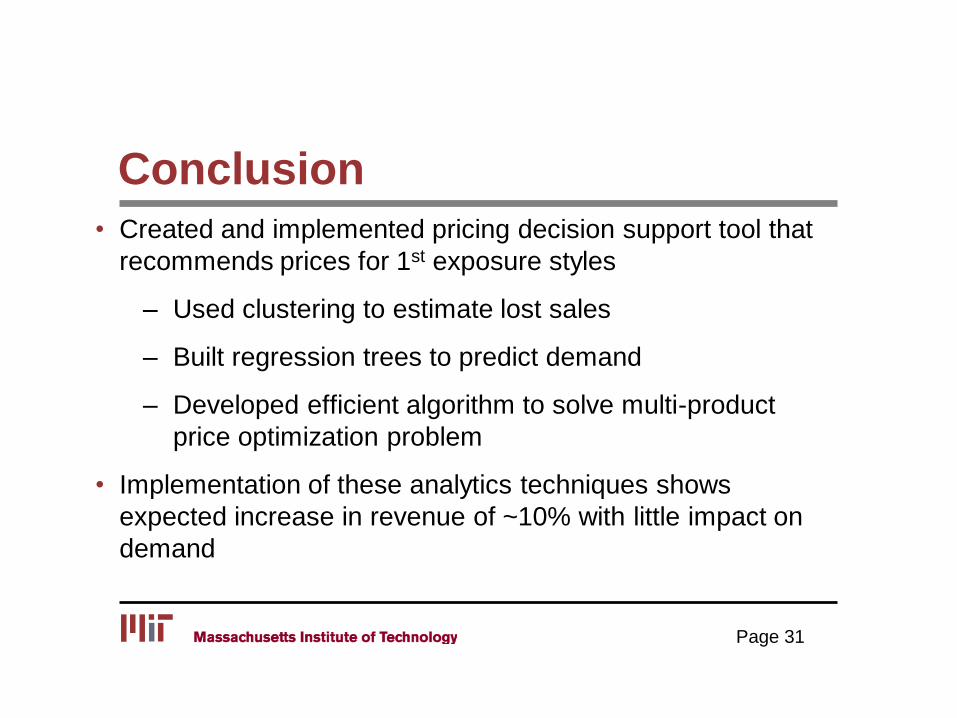
Conclusion
• Created and implemented pricing decision support tool that
recommends prices for 1st exposure styles
– Used clustering to estimate lost sales
– Built regression trees to predict demand
– Developed efficient algorithm to solve multi-product
price optimization problem
• Implementation of these analytics techniques shows
expected increase in revenue of ~10% with little impact on
demand
Page 31

Our Team
Murali Narayanaswamy – VP Pricing & Strategy
Philip Roizin – Chief Financial Officer
Jonathan Waggoner – Chief Operating Officer
Kris Johnson – Operations Research Center
Alex Lee – Systems Design & Management
David Simchi-Levi – Operations Research Center
Deb Mohanty
Hemant Pariawala
Marjan Baghaie, Andy Fano
Paul Mahler, Matt O’Kane
Page 32