Routing Optimization under Uncertaintyjaillet/general/RoutingOptimizationUncertainty-2015.pdf ·...

Accepted for publication in Operations Research, October 2015

Routing Optimization under Uncertainty

Patrick JailletDepartment of Electrical Engineering and Computer Science

Laboratory for Information and Decision Systems

Operations Research CenterMassachusetts Institute of Technology

Cambridge, MA 02139

Email: [email protected]

Jin QiDepartment of Industrial Engineering and Logistics Management

Hong Kong University of Science and Technology

Clear Water Bay, Kowloon, Hong Kong


Melvyn SimDepartment of Decision Sciences, NUS Business School

National University of SingaporeSingapore 119077


We consider a class of routing optimization problems under uncertainty in which all decisions are made

before the uncertainty is realized. The objective is to obtain optimal routing solutions that would, as much

as possible, adhere to a set of specified requirements after the uncertainty is realized. These problems

include finding an optimal routing solution to meet the soft time window requirements at a subset of

nodes when the travel time is uncertain, and sending multiple capacitated vehicles to different nodes to

meet the customers’ uncertain demands. We introduce a precise mathematical framework for defining and

solving such routing problems. In particular, we propose a new decision criterion, called the Requirements

Violation (RV) Index, which quantifies the risk associated with the violation of requirements taking into

account both the frequency of violations and their magnitudes whenever they occur. The criterion can

handle instances when probability distributions are known, and ambiguity, when distributions are partially

characterized through descriptive statistics such as moments information. We develop practically efficient

algorithms involving Benders decomposition to find the exact optimal routing solution in which the RV

Index criterion is minimized, and give numerical results from several computational studies that show the

attractive performance of the solutions.

Key words : vehicle routing, uncertain travel time, robust optimization

1

Jaillet et al.: Routing Optimization under Uncertainty2 Article accepted, Operations Research, October 2015; to appear

1. Introduction

Routing optimization problems on networks consist of finding paths (either simple paths, closed

paths, tours, or walks) between nodes of the networks in an efficient way. These problems and

their solutions have proved to be essential ingredients for addressing many real-world decisions in

applications as diverse as logistics, transportation, computer networking, Internet routing, to name

a few.

In many of these routing applications, the presence of uncertainty in the networks (e.g., arc

travel times, demand requirements, customer presence) is a critical issue to consider explicitly if

one hopes to provide solutions of practical value to the end users. There are two related issues: (i)

how to properly model uncertainty in order to reflect real-world concerns, and (ii) how to do so in

models which will be computationally tractable? In this paper, we provide novel ways to address

such issues for a subclass of these routing problems under uncertainty by using the distributionally

robust optimization framework.

More specifically, we propose a general framework for routing optimization problems where the

objective is to obtain optimal routing solutions that would, as much as possible, adhere to a set of

specified requirements after the uncertainty is realized. We provide an example of finding an optimal

routing solution to meet soft time window requirements at a subset of nodes when travel time is

uncertain. Our model is static in the sense that routing decisions are made prior to the realization of

uncertainty. Instead of defining an exact probability distribution P for the uncertainties, we assume

the true distribution lies in a distributional uncertainty set denoted by F, which is characterized

by some descriptive statistics, e.g., bounded support and moments. Hence, knowing the exact

distribution is only a special case, where F = P. The goal is to find optimal routing solutions

that would mitigate the risks of violations of a set of requirements in a mathematically precise way

via an appropriately defined performance measure, which takes into account such distributional

uncertainty assumptions.

This framework can be applied to transportation networks, for example, for delivery service

providers to route their vehicles, where multiple vehicles and capacity constraints can be incorpo-

rated, or for individuals to make their travel plans.

Related work

The deterministic version of many routing optimization problems (e.g., shortest path problems,

traveling salesman problems, vehicle routing problems) has been studied extensively over many

decades (see the literature reviews of Toth and Vigo, 2002; Oncan et al., 2009; and Laporte, 2010, to

name a few). Due to the recognized practical importance of incorporating uncertainty, the uncertain

Jaillet et al.: Routing Optimization under UncertaintyArticle accepted, Operations Research, October 2015; to appear 3

version of routing problems has also attracted increasing attention. Researchers have formulated

various problems depending on the uncertainty under consideration; for example, uncertainty in

customer presence (see for instance, Jaillet, 1988; Jaillet and Odoni, 1988; Campbell and Thomas,

2008), uncertainty in demand (see for instance, Bertsimas, 1992; Bertsimas and Simchi-Levi, 1996;

Sungur et al., 2008; Gounaris et al., 2013), and uncertainty in travel time (see for instance, Russell

and Urban, 2008; Chang et al., 2009; Li et al., 2010). A comprehensive overview can be found in

Cordeau et al. (2007), Hame and Hakula (2013).

With uncertain arc travel times, and the time window requests at a subset of nodes, the problem

consists of finding paths from the origin to the destination in such a way that the time window

requirements are “effectively” met. However, to the best of our knowledge, only few studies consider

such general routing problems with time windows in the presence of uncertain travel times. At the

heart of the problem, one has to (i) explicitly and quantitatively define the word “effectively”, and

(ii) model the uncertainty.

There are various routing optimization models that handle stochastic travel times. A chance

constrained programming model minimizes the transportation cost while guaranteeing that the

arrival times are within the time windows with a pre-specified probability (Jula et al., 2006; Chang

et al., 2009; Mazmanyan and Trietsch, 2009; Li et al., 2010). This approach is insensitive to the

extent of time window violations and may rule out desirable solutions. For instance, everything else

being equal, a path with a delay probability of 0.011 would be less preferred over another one with a

delay probability of 0.01 even if the delays are 10 minutes and 10 hours, respectively. Other models

include minimizing a combination of expected travel costs and the penalty for violation of the

time windows (Russell and Urban, 2008; Tas et al., 2013, 2014). Notably, routing models that deal

with uncertainty often pose significant computational challenges compared to their deterministic

counterparts (see for instance, Nikolova et al., 2006; Nie and Wu, 2009; Kosuch and Lisser, 2009).

In particular, the computational difficulty with regard to optimization is compounded by the fact

that evaluating the probability that a sum of random travel times is less than a specified level is

already an intractable problem (Khachiyan, 1989; Ben-Tal et al., 2009).

Various robust routing optimization models with travel time uncertainty are proposed in Kou-

velis and Yu (1997), Karasan et al. (2001), Averbak and Lebedev (2004), Montemanni et al. (2004),

Aissi et al. (2005), Woeginger and Deinekoa (2006), Montemmani et al. (2007), Cho et al. (2010),

Catanzaro et al. (2011). Ordonez (2010) provides a comprehensive review. In these robust optimiza-

tion models, uncertain parameters are characterized by uncertainty sets without any information on

their probability distributions. The budget of uncertainty robust optimization approach introduced

by Bertsimas and Sim (2003, 2004) has been adopted to address routing optimization problems

(see Sungur et al., 2008; Souyris et al., 2007; Agra et al., 2013; and Lee et al., 2012). Although these


robust optimization models are more computationally amiable than their stochastic counterparts,

they may represent uncertainty inadequately and result in possibly conservative solutions.

Our contributions

Our main contributions are summarized as follows.

• Given a set of requirements associated with a routing optimization problem, we propose a new

criterion, termed as the Requirements Violation (RV) Index, which evaluates the violation risk of

a solution in meeting these requirements collectively. The criterion possesses important properties

for coherent decision making and accounts for both the frequency and magnitude of requirement

violations by limiting the probabilities of violations as the magnitudes of violations increase.

• Our model of uncertainty is based on probability distributions or distributional ambiguity.

This approach has the benefits of incorporating distributional information and hence results in less

conservative solutions than the classical robust optimization approach where probability distribu-

tions are ignored.

• We propose a precise mathematical framework for a routing optimization problem with a set of

requirements to be fulfilled under uncertainty. We provide a detailed explanation of its application

to the problem of finding an optimal routing solution to meet soft time window requirements at a

subset of nodes when travel time is uncertain. We also provide in the Appendix another application,

corresponding to the problem of sending multiple capacitated vehicles to different nodes to meet

customers’ uncertain demands .

• We develop practically efficient algorithms to find the exact optimal routing solution through

decomposition techniques. Our computational studies also provide the benefit of this approach by

benchmarking against other solution methodologies.

Overview of the paper

The paper is structured as follows. In Section 2, we introduce a new decision criterion, the RV

Index, to evaluate the risk associated with an uncertain attribute violating the requirements, and

present its important properties. In Section 3, we propose a mathematical framework and its

application on the uncertain travel times. In Section 4, we discuss the solution procedure through

decomposition techniques. We also explain a special case, the shortest path problem with deadline,

which is polynomial-time solvable under our criterion when travel times are independent of each

other. In Section 5, we perform several computational studies with encouraging results on the

performance of the RV Index solutions. In Section 6, we briefly discuss how one can extend this

model and framework to account for correlations among uncertain parameters. The proofs of all

the results in the different sections have been grouped together in the Appendix.


Notation

We adopt the following notations throughout the paper. The cardinality of a set N is denoted by

|N |. We use boldface lowercase characters to represent vectors, for example, x= (x1, x2, . . . , xn)′,

and x′ represents the transpose of a vector x. Given a vector x, we define (yi,x−i) to be the vector

with only the ith component being changed, i.e., the vector (yi,x−i) = (x1, . . . , xi−1, yi, xi+1, . . . , xn)′.

We use tilde ( . ) to denote uncertain parameters/attributes, for example, t represents an uncer-

tain travel time. We model uncertainty by a state-space Ω and a σ−algebra F of events in Ω. We

define V as the corresponding space of real-valued random variables. To incorporate distributional

ambiguity, instead of specifying the true distribution P on (Ω,F), we assume that it belongs to a

distributional uncertainty set F, as P ∈ F. We denote by EP(t)

the expectation of t under proba-

bility distribution P. The inequality between two uncertain parameters t≥ v describes state-wise

dominance, i.e., t(ω)≥ v(ω) for all ω ∈Ω. The inequality between two vectors x≥ y corresponds

to the element-wise comparison.

2. Requirements Violation Index

Let t represent a random variable associated with an uncertain attribute of a routing solution

such as the arrival time or the accumulated demand at a node on the network. We would like to

evaluate how well this attribute would adhere to a specified upper limit τ ∈ (−∞,∞] and lower

limit τ ∈ [−∞,∞). Inspired by the Riskiness Index of Aumann and Serrano (2008), we propose the

Requirements Violation Index to quantify the risk associated with an uncertain attribute violating

the requirements.

Definition 1 Requirements Violation (RV) Index: Given an uncertain attribute t and its

lower and upper limits, τ , τ , we define the RV Index ρτ,τ(t)

: V → [0,∞] as follows:

ρτ,τ(t)

= infα≥ 0

∣∣ Cα (t)≤ τ ,Cα (−t)≤−τ ,or ∞ if no such α exists, where Cα

(t)

is the worst-case certainty equivalent under exponential

disutility defined as

Cα(t)

=

supP∈F

α lnEP

(exp

(t

α

))if α> 0,

limγ↓0

Cγ(t) if α= 0,

with α as the risk tolerance parameter.

The concept of worst-case certainty equivalent was proposed by Gilboa and Schmeidler (1989), for

situations where we know that the true distribution of a random variable belongs to a distributional

uncertainty set, i.e., P ∈ F. In our context, this corresponds to the lowest possible deterministic


value of an uncertain attribute t perceived by an individual under Constant Absolute Risk Aversion

(CARA) with risk tolerance parameter α, when evaluated over the ambiguous set of distributions,

F. When t is deterministic, we get Cα(constant) = constant for all α≥ 0. When t follows a known

probability distribution, function Cα(t) can be calculated through the moment generating function

of t. For example, if t follows a normal distribution, i.e., N(µ,σ2), we have Cα(t) = µ+ 12ασ2.

Lemma 1. The worst-case certainty equivalent has some useful properties that we list here:

(a) Cα(t)

is decreasing in α≥ 0 and strictly decreasing when t is not constant. Moreover,

limα↓0

Cα(t) = tF, limα→∞

Cα(t) = supP∈F

EP(t),

where tF = inft∈<|P(t≤ t

)= 1,∀ P∈ F;

(b) For any λ∈ [0,1], t1, t2 ∈ V, and α1, α2 ≥ 0,

Cλα1+(1−λ)α2

(λt1 + (1−λ)t2

)≤ λCα1

(t1)

+ (1−λ)Cα2

(t2)

;

(c) If the random variables t1, t2 ∈ V are independent of each other, then for any α≥ 0,

Cα(t1 + t2

)=Cα

(t1)

+Cα(t2).

Property (a) shows that function Cα(·) is monotonic in α, that is, the smaller the risk tolerance

parameter α is, the larger the certainty equivalent will be. Property (b) indicates that the function

Cα(t)

is jointly convex in(α, t). Property (c) provides a very attractive property for optimization,

with Cα(t) being additive for independent random variables.

Remark 1. To differentiate the “importance” of meeting requirements, we can associate weights

w1,w2 ∈ <+ to the upper and lower limit requirements, respectively, and extend the RV Index

ρτ,τ(t)

: V → [0,∞] to the following definition:

ρτ,τ(t)

= infα≥ 0

∣∣Cw1α

(t)≤ τ ,Cw2α

(−t)≤−τ

.

When w1 ↓ 0, we have for any α≥ 0, limw1↓0Cw1α

(t)

= tF. The requirement would be very harsh,

since it requires that the worst-case realization of t should be no greater than the upper bound

tF. This is consistent with the traditional robust formulation. When w1 →∞, we have for any

α> 0, limw1→∞Cw1α

(t)

= supP∈F EP(t). In that case, the requirement would only impose that the

worst-case expectation should be no greater than the upper bound. For notational simplicity, we

only focus on the case when w1 = w2 = 1. The following analysis however remains valid for the

general case where w1,w2 ∈<+.

To motivate the RV Index as a coherent decision criterion for evaluating how well uncertain

attributes would satisfy the requirements, we present several important properties as follows.


Proposition 1 The RV Index satisfies the following properties for all t, t1, t2 ∈ V:

(a) Full satisfaction: ρτ,τ(t)

= 0 if and only if P(t∈ [τ , τ ]

)= 1 for all P∈ F;

(b) Abandonment: If supP∈F EP(t)> τ or infP∈F EP

(t)< τ , then ρτ,τ

(t)

=∞;

(c) Convexity: For any β ∈ [0,1], ρτ,τ(βt1 + (1−β)t2

)≤ βρτ,τ

(t1)

+ (1−β)ρτ,τ(t2);

(d) Probabilistic bounds: If ρτ,τ(t)≥ 0, we have for all P∈ F,

maxP(t≤ τ − θ

),P(t≥ τ + θ

)≤ exp

(−θ/ρτ,τ

(t)), ∀ θ > 0,

where we follow the standard convention and define θ0

=∞ for any θ > 0.

The full satisfaction property indicates that an uncertain attribute that is guaranteed to satisfy

the requirements (almost surely), irrespective of the choice of the probability measure in F is most

preferred. The abandonment property implies that, unless the uncertain attribute is within the

lower and upper limits in worst case expectation, the RV Index will be infinite, essentially indicating

that this uncertain attribute should be dropped from further consideration. The convexity property

serves two purposes. First, it is synonymous with risk pooling and diversification preference in

the context of risk management. If two random profiles, t1 and t2 are preferred over the profile

t3, then any convex combination of these two profiles will be preferred over t3. Moreover, as we

will illustrate later, it has important ramifications in the context of formulating a computationally

attractive problem which we can use to find optimal solutions via standard solvers. The fourth

property specifies the bounds for the probability of violations. Different from the chance constrained

formulation, which can only guarantee the probability of violation at one specific level without

accounting for the magnitude of violation, the RV Index provides bounds for the probability of

violations at any levels. As a result, a smaller ρτ,τ(t)

provides a lower bound for the probability

of violation.

Collective RV Index

We have motivated the RV Index as a tractable and reasonable alternative to evaluate how well an

uncertain attribute would stay within its specified limits. For instance, in the context of the vehicle

routing problem with soft time windows, the RV Indices at nodes may be used to account for service

deficiencies experienced by the customers due to the violation of time-windows. Naturally, in the

presence of multiple agents (customers), a multi-objective perspective may be more appropriate in

the class of routing problems we are addressing. In that case, the onus would be on the modeler

to specify an appropriate objective function to articulate the tradeoffs among different agents. We

consider an index set I, a set of uncertain attributes, ti, and their requirements to be in [τ i, τ i],

for any i ∈ I. Instead of proposing a specific objective function, we define a Collective RV Index

ρτ ,τ(t)

as follows.


Definition 2 We let α= (αi)i∈I be a vector of nonnegative real-valued parameters. The Collective

RV Index ρτ ,τ(t)

: V |I|→ [0,∞] is defined as

ρτ ,τ(t)

= infϕ(α)

∣∣Cαi (ti)≤ τ i,Cαi (−ti)≤−τ i, αi ≥ 0, i∈ I,

or ∞ if no such α exists. Function ϕ(α) is a subdifferentiable mapping [0,∞]|I|→ [0,∞], which

is non-decreasing and convex in α ≥ 0, with boundary conditions ϕ(0) = 0, and for any j ∈ I,

ϕ ((∞,α−j)) = limαj→∞

ϕ ((αj,α−j)) =∞.

To motivate the Collective RV Index as a reasonable criterion for evaluating how well the uncer-

tain attributes meet the requirements, we next present three important properties of this criterion.

Proposition 2 The Collective RV Index ρτ ,τ(t)

satisfies the following properties.

(a) Full satisfaction: If P(t∈ [τ ,τ ]

)= 1 for all P ∈ F, then ρτ ,τ

(t)

= 0. For any t ∈ V, if

there exists j ∈ I such that P(tj ∈ [τ j, τ j]

)= 1 for all P ∈ F, then ρτ ,τ

((tj, t−j)

)= ρτ ,τ

((tj, t−j)

)for any tj ∈ [τ j, τ j];

(b) Abandonment: If there exists j ∈ I, such that supP∈F EP(tj)> τ j or infP∈F EP

(tj)< τ j,

then ρτ ,τ(t)

=∞;

(c) Convexity: For any t, t0 ∈ V and β ∈ [0,1], ρτ ,τ(βt+ (1−β)t0

)≤ βρτ ,τ

(t)

+ (1 −β)ρτ ,τ

(t0).

The full satisfaction property would ensure that, if all uncertain attributes completely meet

their requirements almost surely, then the index is zero. Furthermore, if there exists one uncertain

attribute that can completely meet the corresponding requirements almost surely, then the Col-

lective RV Index would be insensitive to that attribute. The abandonment property would imply

that, if one of the uncertain attributes violates one of its requirements in expectation (for at least

one P), then the index becomes infinite. The convexity property allows the use of optimization to

its fullest strength toward tractable models.

To ensure these properties, function ϕ (α) is defined in a general sense, and there are many

possibilities for such an index. For example, one can define the function as ϕ (α) = maxi∈I αi or

assign positive weights as ϕ (α) =∑

i∈I wiαi. Specifically, we focus on a special case of the Collective

RV Index named the Additive Collective RV Index as

ρτ ,τ(t)

= inf

∑i∈I

αi

∣∣∣∣∣Cαi (ti)≤ τ i,Cαi (−ti)≤−τ i, αi ≥ 0, i∈ I

.

The algorithm discussed later on could also be applied to the general case. Lam et al. (2013)

introduce a shortfall-aware criterion that is inspired by the joint probability of a set of attributes in

meeting their targets. While the criterion has similar features with the Collective RV Index, it lacks

the property of convexity, which enables us to build tractable models for the routing optimization

problems.


3. General Framework with the Application

In this section, we propose a general binary optimization problem in which the Additive Collective

RV Index is minimized as follows:

inf∑i∈I

αi

s.t. Cαi(z′si

)≤ τ i, i∈ I,

Cαi(−z′si

)≤−τ i, i∈ I,

αi ≥ 0, i∈ I,s∈ S,

(1)

where z represents a vector of independently distributed random variables or possibly constants,

and s= (si)i∈I are binary decision variables with S ⊆ 0,1N×|I|. This framework can be applied

to solve the vehicle routing problem under the uncertain travel times, which we introduce in the

following subsection and the vehicle routing problem under uncertain demands, which we present

in the Appendix.

Vehicle routing problem under uncertain travel times

We consider a routing optimization model where the travel times along the arcs are uncertain and

there is a subset of nodes with soft time window requirements. This is an off-line routing problem

where the routing decisions are made at the beginning before the realization of uncertainty, and

they will not change dynamically in response to the information updates along the network.

Given a directed network G = (N ,A), we let N = 1, . . . , n represent the set of nodes and A

denote the set of arcs in the network. We use (i, j) and a interchangeably to represent an arc in A.

For any node set N 0 ⊂N , we define the following arc sets

δ+(N 0) = (i, j)∈A : i∈N 0, j ∈N\N 0, δ−(N 0) = (i, j)∈A : i∈N\N 0, j ∈N 0.

We let NR ⊆N be the set of nodes that we need to visit. In addition, among these nodes to be

visited, we define the subset ND ⊆NR as the set of nodes with time window impositions. Without

loss of generality, node 1 ∈ NR\ND and node n ∈ ND represent the origin and destination nodes

respectively. Hence, we have δ+(n) = ∅ and δ−(1) = ∅. Two special cases for the set NR are

NR = N , which requires all the nodes in the network to be visited, and NR = ND⋃1, which

corresponds to the situation where only the time window nodes are required to be visited.

Our objective is to determine a routing solution such that the route (a) starts at the origin node

1, ends at the destination node n, (b) visits each node in set NR exactly once, and the rest of

nodes at most once, and (c) effectively respects the time windows specified at nodes in set ND.

We consider the case of soft time windows for which the service at the nodes can start at any time

before or after the time windows. If the vehicle arrives outside of a time window, especially earlier


than the required start time, the vehicle will not wait and will start the service upon its arrival.

This case is suitable for routing in dense urban areas where parking spaces are extremely limited.

To keep things simple, we assume there is only one vehicle available, the travel time along each arc

is independent of each other, and we do not consider the service time at each node.

We let zij represent the uncertain travel time from node i to node j, and decision variables

x∈ 0,1|A| represent the routing decisions. Since the travel times along the arcs are uncertain, the

actual arrival time, at each node i∈N , denoted by ti(x, z), is a function of the decision variables

x and uncertain travel time z, and is therefore also uncertain. If i ∈ ND, then it would be ideal

for the uncertain travel time, ti(x, z) to always fall within the prespecified time window, [τ i, τ i].

However, as such an idealistic solution may not always be feasible, our goal is to find an optimal

routing solution such that arrival times at nodes respect the time windows “as much as possible”,

while keeping the optimization problem tractable from a practical point of view. In order to do

so, we adopt the performance measure that we introduced in Section 2, the RV Index, to evaluate

how the uncertain arrival times respect the corresponding time windows from a systematic point

of view. We formulate a general routing optimization problem under the uncertain travel times as

follows.

inf∑i∈ND

αi

s.t. Cαi (ti(x, z)≤ τ i, i∈ND,Cαi (−ti(x, z)≤−τ i, i∈ND,αi ≥ 0, i∈ND,x∈XRO,

(2)

where

XRO =

x∈ 0,1|A|

∣∣∣∣∣∣∣∣∣∣∣∣∣∣∣∣∣

∑a∈δ+(i)

xa = 1, i∈NR\n,∑a∈δ−(i)

xa = 1, i∈NR\1,∑a∈δ+(i)

xa ≤ 1, i∈N\NR,∑a∈δ−(i)

xa−∑

a∈δ+(i)

xa = 0, i∈N\NR

.

The objective is to minimize the Collective RV Index for all the nodes with time window require-

ments. Set XRO represents the flow conservation constraints, which enforces that each node in the

set NR should be visited exactly once, while the other nodes can be visited at most once.

In Problem (2), the most critical part is the formulation of the arrival time at node i, i.e.,

ti(x, z), which can greatly affect the tractability of the whole model. One classical formulation is

the big-M formulation, which is used in the deterministic vehicle routing problem with deadlines

or time windows (see for instance, Ordonez, 2010). However, this approach does not help us obtain


an equivalent deterministic formulation when uncertainty is present. To evaluate the RV Indices,

the attributes has to be expressed as an affine functions of the underlying uncertainties. Hence, we

introduce a multi-commodity flow formulation to achieve this purpose.

Remark 2. When there is a subset of nodes required to be visited, i.e., NR ⊆N , one intuitive way

to formulate this problem is to convert the current network into a standard network, in which all

the nodes belong to set NR, and the arc travel time is represented by the shortest paths between

each pair of nodes. However, it is worth pointing out that even if the original network is sparse, this

transformation will lead to a complete graph with |NR| (|NR| − 1)/2 arcs, which may increase the

number of decision variables substantially. Interested readers can refer to Cornuejols et al. (1985)

for more details. Besides, the new arc travel times in the transformed network may not necessarily

be independent, even though they were independent in the original one, since the shortest paths

between different pairs of nodes may share common arcs.

Multi-commodity flow formulation

We adapt the multi-commodity flow (MCF) approach to obtain the arrival time at node i, i.e.,

ti(x, z) in Problem (2). We add auxiliary variables si ∈<|A|+ for all i ∈N and for convenience, we

define a |A|× |N | matrix s= (si)i∈N . The formulation is presented as follows.

Proposition 3 Problem (2) can be equivalently written as

inf∑i∈ND

αi

s.t. Cαi(z′si

)≤ τ i, i∈ND,

Cαi(−z′si

)≤−τ i, i∈ND,

αi ≥ 0, i∈ND,(x,s)∈ S,

(3)

where

S =

x∈ 0,1|A|s∈<|A|×|N|+

∣∣∣∣∣∣∣∣∣∣∣∣∣∣∣∣∣∣

x∈XRO, (a)∑a∈δ−(u)

sia−∑

a∈δ+(u)

sia = 0, i∈N\1, u∈N\1, n, i, (b)∑a∈δ+(1)

sia =∑

a∈δ−(i)

xa, i∈N\1, (c)∑a∈δ−(i)

sia−∑

a∈δ+(i)

sia =∑

a∈δ−(i)

xa, i∈N\1, (d)

sia ≤ xa, i∈N\1, a∈A, (e)s1a = 0, a∈A, (f)

. (4)

The commodities in the MCF formulation are fictitious ones and they serve to help us derive the

arrival time at each node as a linear function of the arcs’ travel times, z, which is necessary for us

to compute the certainty equivalents of the uncertain arrival times at the nodes. We consider |N |


commodities with node 1 as the source node and node i as the sink node for commodity i∈N . Here,

the variable sia denotes the amount for commodity i flowing along the arc a, and the formulation

ensures that∑

a∈δ−(i) xa unit of commodity i flows from the source node 1 to the sink node i.

Constraints (4b)-(4d) represent the flow conservation of commodities at all the nodes. Note that if

the path defined by x contains the node i, then∑

a∈δ−(i) xa = 1; otherwise, no commodity would

be sent to the ith node. For example, for commodity i∈NR\1, we need to send∑

a∈δ−(i) xa = 1

(see Problem (2)) unit of commodity i from the source node 1 to the destination node i. Constraint

(4e) ensures that the commodity flow along the arc a is bounded by xa for all arc a∈A. Observe

that while s is not constrained to binary values, we have shown in the proof (see the Appendix)

that all the feasible solutions of s are necessarily binary. Since the flow can only go through the

arc with capacity xa = 1, it will go through the only path determined by xa. Consequently, sia = 1

if and only if commodity i going from node 1 to node i flows on arc a. Hence, a ∈ A : sia = 1

represents the set of arcs on the path to node i and we can express the arrival time at node i∈N

as ti(x, z) = z′si.

The MCF formulation was proposed by Claus (1984), and has been verified as a relatively strong

formulation for the traveling salesman problem in terms of LP relaxation (Oncan et al. 2009).

In total, the MCF formulation has |N ||A|+ |ND| continuous variables, |A| binary variables, and

|N ||A|+ |N |2 + |ND| − 1 (≈O(|N ||A|)) constraints. Besides this MCF formulation, we also have

an alternative formulation in the Appendix that is based on linear decision rule.

The general framework can also be applied to solve the vehicle routing problem under uncertain

demands and we provided a more detailed explanation of this application in the Appendix.

4. Solution algorithm

After observing the problem structure of the above application, we next describe the solution

procedure for the general problem (1). To guarantee the feasibility of the problem, we impose the

restriction that the lower and upper limits τ ,τ , are such that there exists a feasible solution s∈ S

satisfying

supP∈F

EP(z′si

)≤ τ i, sup

P∈FEP(−z′si

)≤−τ i, i∈ I.

This implies that the lower and upper limits must be chosen such as to guarantee that there exists a

feasible solution s in which z′si, i∈ I can stay within the limits in expectation. This assumption is

reasonable since violating it would lead to an infinite optimal value for our formulation, essentially

indicating that the lower and upper limits are unreasonable.


We further study the function Cαi(z′si), and develop algorithms to solve the problem. Given

s∈ S, we define the function f(s) as

f(s) = inf∑i∈I

αi

s.t. Cαi(z′si)≤ τ i, i∈ I,

Cαi(−z′si)≤−τ i, i∈ I,

αi ≥ 0, i∈ I.

(5)

Observing that function Cαi(·) is convex in αi, if Cαi(z′si) can be calculated easily for any given

αi, Problem (5) is a classical convex problem and can be solved efficiently.

We next show that f(s) is convex in s, and concentrate on the calculation of a subgradient of

f(s).

Calculation of a subgradient of f(s)

The Lagrange function L(s,α,λ) of Problem (5) is given by

L(s,α,λ) =∑i∈I

αi +∑i∈I

λi(Cαi(z

′si)− τ i)

+∑i∈I

λi(Cαi(−z

′si) + τ i),

where λi, λi are the Lagrange multipliers associated with the inequality constraints Cαi(−z′si)≤

−τ i and Cαi(z′si)≤ τ i, and we define λ= (λ,λ). We next show the convexity of the function f(s)

and that a subgradient of f(s) can be calculated through its Lagrange function.

Proposition 4 The function f(s) is convex in s, and if the vector

(dLs (s,α∗,λ∗)dLα(s,α∗,λ∗)

)is a subgradi-

ent of the function L(s,α,λ∗) at (s,α∗), and dLα(s,α∗,λ∗) = 0, then dLs (s,α∗,λ∗) is a subgradient

of f(s), where

(α∗,λ∗)∈Z(s) =

(αo,λo)

∣∣∣∣L (s,αo,λo) = supλλλ≥000

infααα≥000

L (s,α,λ)

.

Hence, to calculate a subgradient of f(s), Proposition 4 suggests we can equivalently calculate

dLsss (s,α∗,λ∗). Given s, after solving Problem (5), we calculate a subgradient as follows.

Proposition 5 A subgradient of f(s) with respect to sia for all i∈ I, a∈A can be calculated as

dfsia

(s) =

0, i∈ I1, a∈A,

−dc2sia

(α∗i ,si)

dc2αi (α∗i ,si), i∈ I2, a∈A,

−dc1sia

(α∗i ,si)

dc1αi (α∗i ,si), i∈ I3, a∈A,

(6)

where we separate the set I into three sets.

I1 = i∈ I|α∗i = 0,I2 = i∈ I\I1|Cα∗i (z

′si)< τ i,Cα∗i (−z′si) =−τ i,

I3 = i∈ I\I1|Cα∗i (z′si) = τ i,Cα∗i (−z

′si)≤−τ i.


Function dc1sia

(α∗i ,si) and dc1αi(α

∗i ,s

i) is a subgradient of Cαi(z′si) with respect to sia and αi at point

(α∗i ,si), and dc2

sia(α∗i ,s

i) and dc2αi(α∗i ,s

i) is a subgradient of Cαi(−z′si) with respect to sia and αi at

point (α∗i ,si).

We have shown how to calculate f(s) and its subgradient. Since f(s) is a convex function, we

next approximate it with a piece-wise linear function, and use Benders decomposition algorithm

to solve Problem (1).

Proposition 6 For any y ∈ S, we have

f(y) = supsss∈S

f(s) + dfsss (s)′(y− s)

, (7)

where dfsss (s) is a vector of subgradient of f(s) with respect to s.

As the size of the set S is relatively large for us to directly tackle the problem, we use Benders

decomposition method and summarize the entire algorithm as follows.

Algorithm RO

1. Select any s(0) ∈ S, and set k := 0.

2. Given current solution s(k), solve the convex problem (5) and find the optimal α. Calculate

a subgradient function dfsss(s(k))

according to Equation (6).

3. Solve the following subproblem

inf bs.t. b≥ f(s(i)) + dfsss (s(i))′(s− s(i)), ∀ i= 0, . . . , k,

s∈ S,(8)

and denote the optimal solution by s(k+1) and the optimal value by b∗.

4. If b∗ = f(s(k+1)), then stop and output the optimal solution s∗ = s(k+1).

5. If b∗ < f(s(k+1)), update k← k+ 1, and go to step 2.

Proposition 7 Algorithm RO finds an optimal solution to Problem (7) in a finite number of steps.

In this paper, we do not go further to discuss efficient algorithms for solving this subproblem.

Adulyasak and Jaillet (2014) provides more details and extensive computational results on various

algorithms based on a branch-and-cut framework.

Calculation of Cα(z′s) with different distributional uncertainty sets

We observe that Problem (5) is solvable as long as we can calculate function Cαi(z′si) and its

subgradient for si ∈<|A|+ , which is dependent on the information set of random variables z. We next

present three types of information on the probability distributions of z. For notational simplicity,

we remove the subscript i and present the calculation of function Cα(z′s).


Since z = (za)a∈A is a vector of independent random variables, we have

Cα(z′s) =∑a∈A

Cα(zasa),

where the equality holds since Cα(·) is additive for independent random variables. Observing that

although Cα(zasa) =Cα(za)sa holds when sa ∈ 0,1, Cα(za) is not its subgradient for the general

case when sa ∈ <+. Besides, another subtle issue with expressing Cα(zasa) =Cα(za)sa is that the

expression Cα(za)sa would not be jointly convex in α and sa, and this would violate the condition

for Proposition 4 to hold. Hence, instead of simply using Cα(za) as the subgradient formula, we

show the subgradient calculation for the general case as follows.

Known distribution

When the probability distribution of the random variable za is completely known, the function

Cα(zasa) can be calculated through the moment generating function. For example, if za follows a

normal distribution N(µa, σ2a), the certainty equivalent of zasa is

Cα (zasa) = α lnEP

(exp

(zasaα

))= α ln

(exp

(µasaα

+σ2as

2a

2α2

))= µasa +

σ2as

2a

2α,

and the subgradient can be calculated sequentially as

dcsa(α,s) =∂

∂saCα(z′s) =

∂

∂saCα(zasa) = µa +

σ2a

αsa,

dcα(α,s) =∂

∂αCα(z′s) =

∑a∈A

∂

∂αCα(zasa) =−

∑a∈A

σ2a

2α2s2a.

Discrete distribution with moment information

Suppose that we know the random variable za can only take the discrete values za ∈ za1, . . . , zaKa

and we may have the moment information on za as follows.

Fa =P∣∣∣EP(g(za))∈

[ηa,ηa

],P (za ∈ za1, . . . , zaKa) = 1

,

where function g(za) = (gl(za))l∈L, and gl(za) can be any power of the random variable za, i.e.,

gl(za) = zma , and m is an integer. Given α,sa ∈ <+, the certainty equivalent Cα(zasa) can be

calculated as

Cα(zasa) = α ln supP∈Fa

EP (exp (zasa/α)) = α lnEQa (exp (zasa/α)) ,


where the probability distribution Qa is the optimal solution of the following linear optimization

problem, i.e., Qa ∈ arg supP∈Fa EP (exp (zasa/α)).

supP∈Fa

EP

(exp

(zasaα

))= sup

Ka∑k=1

pak exp(zaksa

α

)s.t.

Ka∑k=1

pakg(zak)≤ ηa,

Ka∑k=1

pakg(zak)≥ ηa,

Ka∑k=1

pak = 1,

pak ≥ 0, k= 1, . . . ,Ka.

Hence, based on Danskin’s Theorem (Danskin, 1967; Bertsekas, 1999), we calculate the subgradient

as

dcsa(α,s) =∂

∂saCα(z′s) =

∂

∂saCα(zasa) =

∂

∂saα lnEQa (exp (zasa/α))=

EQa (exp (zasa/α) za)

EQa (exp (zasa/α)),

dcα(α,s) =∂

∂αCα(z′s) =

∑a∈A

∂

∂αCα(zasa) =

∑a∈A

∂

∂αα lnEQa (exp (zasa/α))

=∑a∈A

(lnEQa (exp (zasa/α))− EQa (exp (zasa/α) zasa)

αEQa (exp (zasa/α))

)Continuous distribution with certain descriptive statistics

When the random variable za is a continuous random variable, and the uncertainty set is represented

as

Fa =P∣∣∣EP (za)∈

[µa, µa

], P (za ∈ [za, za]) = 1

, (9)

where [za, za] is bounded support, we calculate the certainty equivalent based on the following

lemma.

Lemma 2. If the distributional uncertainty set of random variable za is given as Equation (9),

then given α,sa ∈<+

Cα (zasa) = supP∈Fa

α lnEP

(exp

(zasaα

))=

α ln

(g(za) exp

(zasaα

)+h(za) exp

(zasaα

)), α > 0,

zasa, α= 0.,

where g(za) = za−µaza−za

and h(za) =µa−zaza−za

.

Immediately, as the function Cα(z′s) is differentiable, we calculate its gradient with respect to

sa as

dcsa(α,s) =∂

∂saCα(z′s)

=∂

∂saCα (zasa)

=∂

∂saα ln (g(za) exp (zasa/α) +h(za) exp (zasa/α))

=g(za) exp (zasa/α)za +h(za) exp (zasa/α)zag(za) exp (zasa/α) +h(za) exp (zasa/α)

.


When sa = 0, we have∂Cα(z′s)

∂sa

∣∣∣∣sa=0

= µa. Meanwhile, the gradient of Cα(z′s) with respect to α is

dcα(α,s) =∂Cα

(z′s)

∂α=∑a∈A

∂

∂αCα(zasa)

=∑a∈A

ln (g(za) exp (zasa/α) +h(za) exp (zasa/α))

−g(za) exp (zasa/α)za +h(za) exp (zasa/α)zag(za) exp (zasa/α) +h(za) exp (zasa/α)

saα

.

Among these three types of information, two of them are based on the distributional robust opti-

mization framework in which probability distributions are assumed to be unknown and constrained

within an ambiguity set. Different from the classical uncertainty set which excludes the information

on probability distributions, the ambiguity set considers all possible probability distributions that

are characterized by the support set and a given set of descriptive statistics such as means, covari-

ance and possibly higher moments. Therefore, this distributionally robust optimization framework

is potentially as tractable as robust optimization and has the benefit of being less conservative. We

refer interested readers to Wiesemann et al. (2014) for more discussion on it.

A special case: stochastic shortest path problem with deadline

We next discuss a special case where we only specify an upper limit on the travel time at the

destination node. In this case, set I is a singleton, and the corresponding lower and upper limits

are 0 and τ .

ρ0,τ

(z′s)

= infα≥ 0

∣∣Cα (z′s)≤ τ .This criterion is similar to the riskiness index of Aumann and Serrano (2008). It is a particular

case of the satisficing measure proposed by Brown and Sim (2009) and Brown et al. (2012) for

evaluating uncertain monetary outcomes and has been applied in project selection by Hall et al.

(2014). We use the RV Index as an optimization criterion to formulate the problem as follows.

inf ρ0,τ

(z′s)

s.t. s∈ S. (10)

Its computational complexity can be found in the following proposition.

Proposition 8 Problem (10) is polynomial-time solvable when the random variables z are inde-

pendent of each other and its nominal version mins∈S z′s can be solved in polynomial time.

In particular, if the feasible set S is the set for the shortest path problem defined as

SSP =

s∈ 0,1|A|∣∣∣∣∣∣∑

a∈δ+(i)

sa−∑

a∈δ−(i)

sa =

1, when i= 1,−1, when i= n,0, otherwise

,


with the standard convention that a sum of an empty set of indices is 0. The shortest path problem

based on minimizing the RV Index is polynomial-time solvable for independently distributed uncer-

tain arc travel times. For any given α ≥ 0, we can solve mins∈SSP Cα(z′s)

by standard shortest

path algorithms, and then we use a bisection algorithm to find the optimal α. As far as we know,

it possibly is the only formulation that incorporates a deadline, accounts for both probabilistic and

ambiguous distributions of travel times, but still retains a polynomial time complexity.

5. Computational Study

In this section, we conduct computational studies intending to address two concerns. First, whether

this newly proposed RV Index criterion can provide us a reasonable solution under uncertainty.

Second, as the deterministic version of the general routing optimization problems is already hard

to solve, whether the RV Index model is practically solvable. The program is coded in python and

run on a Intel Core i7 PC with a 3.40 GHz CPU by calling CPLEX 12 as ILP solver.

Since the main contribution of this paper is methodological, where we introduce a new criterion

and framework to deal with routing optimization under uncertainty, we have decided to concentrate

our computational study to only one of the possible routing applications, the one dealing with

uncertainty about travel time as described in Section 3. We believe that this will allow the reader

to clearly understand our proposed framework and get a sense of how it compares with well-

documented other existing methods. In this computational study, we will also restrict ourselves

to the case where the time window is only composed of a deadline, i.e., ignoring the lower limit

bounds.

Benchmarks for stochastic shortest path problem with deadline

We carry out the first experiment to make a comparative study on the validity of the RV Index

as a decision criterion. For a randomly generated network, we solve a shortest path problem with

deadline under uncertainty, in which ND = n and NR = 1, n. We investigate several classical

selection criteria to find optimal paths, and then use out-of-sample simulation to compare the per-

formances of these paths. Let z = (za)a∈A represent the independently distributed arc travel times

and EP(z) =µ, z ∈ [z,z]. We summarize four selection criteria which appeared in the literature.

Minimize average travel time

For a network with uncertain travel time, the simplest way to find a path is by minimizing the

average travel times, which can be formulated as a deterministic shortest path problem.

mins∈SSP

µ′s.

This problem is polynomial-time solvable, but the optimal path does not depend on the deadline.


Maximize arrival probability

The second selection criterion is to find a path that gives the largest probability to arrive on time,

which is formulated as follows:

maxs∈SSP

P(z′s≤ τ

)Since the problem is intractable (Khachiyan, 1989), we adopt a sampling average approximation

method to solve it. Assuming the sample size is K, then we solve

max1

K

K∑k=1

Ik

s.t. s′zk ≤M(1− Ik) + τ , k= 1, . . . ,K,Ik ∈ 0,1, k= 1, . . . ,K,s∈ SSP ,

where M is a big number.

Maximize punctuality ratio

The third selection criterion is to maximize the punctuality ratio, which is defined as

maxs∈SSP

τ −µ′sσ(z′s) (11)

where σ(·) represents the standard deviation. The idea is to find a path that can give a shorter and

less uncertain travel time. When the travel time on each arc is independently normally distributed,

maximizing the arrival probability is in fact equivalent to maximizing the punctuality ratio, since

P(z′s≤ τ

)= P

(z′s−µ′sσ(z′s) ≤ τ −µ′s

σ(z′s))= Φ

(τ −µ′sσ(z′s)) ,

in which, Φ(·) is the cumulative distribution function of the standard normal random variable

N(0,1). As this problem is not a convex problem, we use the algorithm proposed by Nikolova et al.

(2006) to solve it. They show that the objective function is quasi-convex on a subset of feasible set

SSP = SSP ∩ s|µ′s< τ, and prove the maximum is attained at an extreme point of SSP . Then

we can enumerate all the extreme points with the bisection method and start with two end points:

the point which returns the path with smallest mean, and the point that returns the path with

smallest variance.

Maximize budget of uncertainty

By introducing a parameter Γ, named budget of uncertainty, Bertsimas and Sim (2003, 2004)

provide a new robust formulation to flexibly adjust the level of conservatism while withstanding

the parameter uncertainty. This formulation can also be applied readily to discrete optimization

problems (Bertsimas and Sim, 2003). Hence, the robust shortest path problem is formulated as

mins∈SSP

maxz∈WΓ

z′s


in which,WΓ =

µ+ c

∣∣∣∣∣0≤ c≤ z−µ,∑a∈A

caza−µa

≤ Γ

, for all Γ≥ 0. Γ = 0 represents the nominal

case. Given the deadline τ , we transform the problem to find a path that can return the maximal

Γ while respecting the deadline. The formulation is given as

Γ∗ = max Γs.t. max

z∈WΓ

z′s≤ τ ,

s∈ SSP .

Following the calculation procedure suggested by Bertsimas and Sim (2003), we first define 0 =

z|A|+1−µ|A|+1 ≤ z|A|−µ|A| ≤ . . .≤ z1−µ1 ≤∞, and the above problem is equivalent to

Γ∗ = max Γs.t. min

l=1,...,|A|+1Γ(zl−µl) +Cl ≤ τ ,

where Cl = minsss∈SSP

(µ′s+

∑l

j=1 ((zj −µj)− (zl−µl))sj), l = 1, . . . , |A|+ 1, which is a classical

shortest path problem. After solving |A|+ 1 shortest path problems, we get

Γ∗ = maxl=1,...,|A|+1

τ −Clzl−µl

.

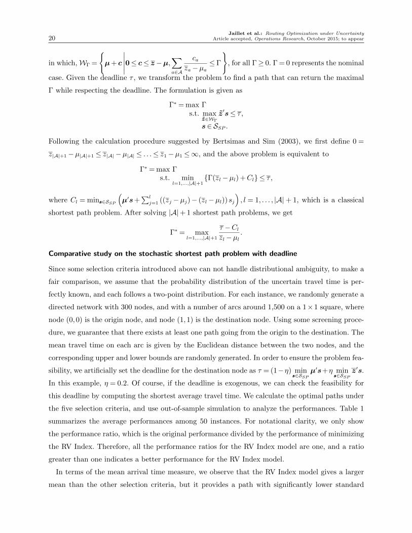
Comparative study on the stochastic shortest path problem with deadline

Since some selection criteria introduced above can not handle distributional ambiguity, to make a

fair comparison, we assume that the probability distribution of the uncertain travel time is per-

fectly known, and each follows a two-point distribution. For each instance, we randomly generate a

directed network with 300 nodes, and with a number of arcs around 1,500 on a 1×1 square, where

node (0,0) is the origin node, and node (1,1) is the destination node. Using some screening proce-

dure, we guarantee that there exists at least one path going from the origin to the destination. The

mean travel time on each arc is given by the Euclidean distance between the two nodes, and the

corresponding upper and lower bounds are randomly generated. In order to ensure the problem fea-

sibility, we artificially set the deadline for the destination node as τ = (1−η) minsss∈SSP

µ′s+η minsss∈SSP

z′s.

In this example, η = 0.2. Of course, if the deadline is exogenous, we can check the feasibility for

this deadline by computing the shortest average travel time. We calculate the optimal paths under

the five selection criteria, and use out-of-sample simulation to analyze the performances. Table 1

summarizes the average performances among 50 instances. For notational clarity, we only show

the performance ratio, which is the original performance divided by the performance of minimizing

the RV Index. Therefore, all the performance ratios for the RV Index model are one, and a ratio

greater than one indicates a better performance for the RV Index model.

In terms of the mean arrival time measure, we observe that the RV Index model gives a larger

mean than the other selection criteria, but it provides a path with significantly lower standard


Selection criteriaPerformance measures

MeanLateness

STDEV1 EL2 CEL3 VaR VaRCPU time

probability @95%4 @99%

Minimize average travel time 0.9845 1.1236 1.2061 1.3965 1.2279 1.0056 1.0138 0.0267Maximize arrival probability 1.0064 1.5491 1.1163 1.8732 1.2023 1.0167 1.0213 926.1399Maximize punctuality ratio 0.9864 1.0329 1.1498 1.2010 1.1565 1.0019 1.0082 1.2552Maximize budget of uncertainty 0.9896 1.1252 1.1549 1.3254 1.1595 1.0047 1.0102 44.8723Minimize the RV Index 1 1 1 1 1 1 1 11 STDEV refers to standard deviation;2 EL refers to expected lateness, EL=EP

((z′s∗− τ)+

);

3 CEL refers to conditional expected lateness, CEL=EP((z′s∗− τ)+ |z′s∗ > τ

);

4 VaR@γ refers to value-at-risk, VaR@γ = infν ∈<|P(z′s∗ > ν)≤ 1− γ .

Table 1 Performances of various selection criteria for the stochastic shortest path problem with deadline.

deviation, expected lateness and conditional expected lateness. Hence, by slightly increasing the

expected travel time, the RV Index model can better mitigate the risk of tardiness. In addition,

since solving the stochastic shortest path problem under the RV Index only requires solving a small

sequence of deterministic shortest path problems, the CPU time is relatively short compared to

the other methods, except for the selection criterion of minimizing the average travel time. For

maximizing the arrival probability, since we use a sampling average approximation, the calculation

takes quite a long time even with a small sample size (K = 80), and the performance is worse even

in terms of the lateness probability.

By varying the coefficient η, we also alter the deadline at the destination node, and summarize

the performance ratio of each selection criterion in Figure 1. We exclude the selection criterion

0.1 0.2 0.3 0.4 0.5 0.6 0.7 0.8 0.90.94

0.95

0.96

0.97

0.98

0.99

1

1.01Mean ratio

d

0.1 0.2 0.30.9

1

1.1

1.2

1.3

1.4

1.5

1.6Lateness probability ratio

d

0.1 0.2 0.3 0.4 0.5 0.6 0.7 0.8 0.90.95

1

1.05

1.1

1.15

1.2

1.25

1.3Standard deviation ratio

d

0.1 0.2 0.30.8

1

1.2

1.4

1.6

1.8

2

2.2Expected lateness ratio

d

RV index Budget of uncertainty Punctual ratio Mean

Figure 1 Performance comparison for the stochastic shortest path problem when deadline varies.

of maximizing the arrival probability, as a small sample size resulted in inconsistent solutions for


comparison. Among the remaining four selection criteria, the RV Index model outperforms the

others, especially in terms of standard deviation. It is worthwhile to point out that in terms of the

lateness probability ratio and expected lateness ratio, η is only used with values 0.1,0.2,0.3, since

when η is greater than 0.3, the lateness probability and expected lateness under the RV Index

solution are very close to 0. A similar conclusion can be derived when the travel times are uniformly

distributed.

Since the shortest path problem with deadline is a special case of our more general routing prob-

lem, we can also test the algorithm RO of Section 4 on it, though it is not necessarily polynomial-

time solvable. We randomly generate 50 instances, and compare the statistics on CPU time of

these two algorithms for a network with 300 nodes and 1,500 arcs. Table 2 suggests the calcula-

tion time of RO algorithm is longer than the bisection method, but is still attractive. It provides

an encouraging result for the employment of RO algorithm in the general routing optimization

problem.

StatisticsBisection RO algorithm

CPU time (sec) CPU time (sec) Number of iterations

Average 0.396 1.211 3.32Maximum 0.512 4.951 14Minimum 0.165 0.356 1Standard deviation 0.059 1.093 3.01

Table 2 Statistics of CPU time of two algorithms for the stochastic shortest path problem with deadline.

5.1. Illustration of the solution procedure on the general routing optimization problem

We next consider an example on a simple network with 5 nodes and 12 arcs shown in Figure 2, and

provide a detailed description of the results obtained using the Collective RV Index, as well as the

computational characteristics of our proposed solution methodologies. We assume that the travel

time follows continuous distribution and only the mean and bounded supports are known. The

information is specified in Table 3. The travel time uncertainties along the arcs vary according

Index Arc Lower bound Mean Upper bound Index Arc Lower bound Mean Upper bound

1 (1,2) 2(1−β) 2 2(1 +β) 7 (3,2) 2(1−β) 2 2(1 +β)2 (1,3) 2(1−β) 2 2(1 +β) 8 (3,4) 2(1−β) 2 2(1 +β)3 (1,4) 2(1−β) 2 2(1 +β) 9 (3,5) 1−β 1 1 +β4 (2,3) 3(1−β) 3 3(1 +β) 10 (4,2) 6(1−β) 6 6(1 +β)5 (2,4) 7(1−β) 7 7(1 +β) 11 (4,3) 4(1−β) 4 4(1 +β)6 (2,5) 4(1− 1.5β) 4 4(1+1.5β) 12 (4,5) 7(1−β) 7 7(1 +β)

Table 3 Travel time information corresponding to Figure 2.

to the parameter β. Note that arc 6 is distinct from the rest. Our aim is to find a path from

node 1 to node 5, that visits each node exactly once, and meets the specific deadline requirements


1"

2" 3"

4"

5"

Figure 2 A simple network with five nodes.

τ3 = τ5 = 14.5. Correspondingly, ND = 3,5 and NR =N . In this simple network, if we ignore the

deadline constraints, all the feasible paths can be easily enumerated as in Table 4.

Index Path

1 1→ 2→ 3→ 4→ 52 1→ 2→ 4→ 3→ 53 1→ 3→ 2→ 4→ 54 1→ 3→ 4→ 2→ 55 1→ 4→ 2→ 3→ 56 1→ 4→ 3→ 2→ 5

Table 4 All feasible paths for the illustrative example without the deadline requirements.

By substituting the uncertain travel times with their mean values, paths 1, 2, 4, 5, and 6 are

all feasible paths that can meet the deadline requirements. Instead, when the travel times take

their worst values, we can see that, if β = 0.1, both paths 5 and 6 would satisfy the deadline

requirements. If β = 0.2, only path 5 is feasible, and no path is feasible when β = 0.3,0.4. The result

indeed illustrates that the worst case approach may be overly conservative. With the Collective

RV Index, when β = 0.1,0.2, the selection decisions are the same as the worst-case method, and

the associated objective value is 0. When β = 0.3,0.4, the calculation procedure is listed in Table

5.

Several interesting results can be observed from this computational study. With the increase

of β, travel time becomes more uncertain, and the optimal path changes from path 5 to path 6.

Observing that node 3 has the same deadline as the destination node 5, intuitively, travelers may

expect that as long as node 3 can be reached before the destination node, the actual time of arrival

would be inconsequential. However, the obtained result is not so trivial. When β = 0.3, as shown

in Table 6, even the worst-case arrival time at node 3 through both path 5 and path 6 can meet

the presumed deadline. Therefore, with the full satisfaction property of the Collective RV Index,

the selection decision only depends on whether the arrival time meets the deadline at node 5, and

path 5 is calculated as optimal. Similarly, when β = 0.4, the value of the Collective RV Index of


β Iterationoptimal solution objective value optimal alpha summation of optimal alpha(path number) w∗ (α∗2, α

∗5) f(y∗)

0.3

0 5 (0,0.448) 0.4481 6 −1.024 (0,0.710) 0.7102 1 0.191 (0,5.844) 5.8443 2 0.360 (1.785,6.209) 7.9944 5 0.448 (0,0.448) 0.448

0.4

0 5 (0.439,1.137) 1.5761 6 −5.650 (0,1.551) 1.5512 1 −0.459 (0,10.464) 10.4643 2 0.678 (3.397,11.109) 14.5064 6 1.551 (0,1.551) 1.551

Table 5 Calculation procedure of the Collective RV Index model with different β.

path 6 only depends on the performance at node 5. Nonetheless, when traveling through path 5,

the Collective RV Index should account for both node 3 and node 5. Accordingly, path 6 becomes

the optimal path.

β NodePath 5 Path 6

Lower bound Mean Upper bound Lower bound Mean Upper bound

0.33 7.7 11 14.3 4.2 6 7.85 8.4 12 15.6 7.8 12 16.2

0.43 6.6 11 15.4 3.6 6 8.45 7.2 12 16.8 6.4 12 17.6

Table 6 Arrival time comparison between paths 5 and 6.

Computation results of the general routing optimization problem

The formulation of the routing optimization problem implies that the computation time greatly

depends on the network structure, |N |, |A|, and the properties of sets NR and ND. Additionally,

the deadline setting will also tremendously affect the size of the feasible set, and so, the number

of iterations. In this part, we mainly focus on the influence of the number of nodes and arcs on

the computation time and the number of iterations, and show the results in Table 7 and Table

8 respectively. We randomly generate the arcs for a network while ensuring the existence of a

Hamiltonian path, and the information of uncertain travel times includes means and supports. To

set reasonable deadlines, we first derive a feasible path that minimizes the total average travel

time. With this path, we calculate the corresponding mean arrival time and worst-case arrival time

for each node with a deadline requirement, and set the deadline in between. For each case, we

randomly generate 20 instances, and present the average values.

Table 7 demonstrates that the RO algorithm can solve moderate-size problems within a rea-

sonable time range. While setting the time limit as 7200 seconds, with the MCF formulation,

the RO algorithm can solve a network with 100 nodes, and 450 arcs for the case where NR =

ND⋃1,ND = [n/2], n. Table 8 shows that on average, we only need a relatively small number


G NR =N ,ND =N\1 NR =N ,ND = [n/2], n NR =ND⋃1,ND = [n/2], n

= N ,A Avg Max Min STD Avg Max Min STD Avg Max Min STD

|N |= 10 |A|= 30 0.78 2.00 0.20 0.52 0.45 0.94 0.19 0.25 0.18 0.37 0.13 0.06

|N |= 10 |A|= 50 6.06 17.7 0.72 5.55 1.93 5.52 0.32 1.38 0.41 1.19 0.16 0.29

|N |= 10 |A|= 70 21.7 135 0.72 31.8 5.84 26.0 0.40 6.50 0.58 1.23 0.27 0.31

|N |= 20 |A|= 60 8.59 28.6 1.17 7.57 3.02 8.11 1.18 1.94 1.59 6.77 0.44 1.68

|N |= 30 |A|= 90 55.8 310 5.52 69.3 24.0 96.6 3.37 28.2 6.23 23.7 1.84 6.19

|N |= 40 |A|= 120 854 5002 21.3 1436 134 718 11.8 202 13.3 36.1 4.34 10.1

Table 7 Computation time (sec) on routing optimization problem with different settings.

G = N ,A NR =N ,ND =N\1 NR =N ,ND = [n/2], n NR =ND⋃1,ND = [n/2], n

Avg Max Min STD Avg Max Min STD Avg Max Min STD

|N |= 10, |A|= 30 4.35 10 1 2.50 3 6 1 1.72 1.5 5 1 0.95

|N |= 10, |A|= 50 11.2 30 1 8.83 6.45 12 1 3.62 2.8 8 1 2.07

|N |= 10, |A|= 70 10.9 47 1 12.1 6.1 18 1 5.10 2.8 8 1 1.94

|N |= 20, |A|= 60 11.9 31 1 9.49 4.1 11 1 3.14 2.95 12 1 2.86

|N |= 30, |A|= 90 17.1 43 2 11.5 7.85 27 1 7.44 2.6 9 1 2.04

|N |= 40, |A|= 120 36.8 133 3 36.8 9.55 27 1 7.47 2 5 1 1.30

Table 8 Number of iterations on routing optimization problem with different settings.

of iterations. If more efficient algorithms can be implemented for solving the subproblem, the com-

putation time can be remarkably improved. For example, Adulyasak and Jaillet (2014) introduces

a branch-and-cut algorithm, which greatly reduces the computation time with |N |= 40, |A|= 120

for the second case from 134 seconds to 1.3 seconds. It is also clear that the computation time and

the number of iterations greatly depend on how tight the deadlines are, since tight deadlines imply

a small feasible set.

6. Extension: correlations between uncertainties

Clearly, in practice, the uncertain travel time on each arc, or the uncertain demand from each

customer may be correlated. For example, uncertain travel times may depend on some common

factors, e.g., weather conditions, existence of traffic jam. However, most papers in the relevant

literature dealing with routing optimization under uncertainty have assumed that uncertainties are

independently distributed so as to avoid the tremendous increase in modeling and computational

complexity. As an example, Kouvelis and Yu (1997) has shown that the following robust shortest

path problem

mins∈SSP

maxz′1s,z′2s,

where z1 = (z1a)a∈A,z2 = (z2a)a∈A are two travel time scenarios, is NP-hard. Qi et al. (2015) also

prove that when the arc travel times are correlated, the path selection problem that minimizes the

certainty equivalent of total travel time

mins∈SSP

Cα(z′s)

is NP-hard.


We next provide a possible way to extend our current model to the case in which the uncertain

parameters are correlated. Instead of specifying the commonly used covariance matrix, which may

greatly complicate the model, we assume that these uncertain parameters, e.g., uncertain travel

times or uncertain demands, are an affine function of independently distributed factors c1, . . . , cK ,

i.e.,

za = z0a +

K∑k=1

zka ck, ∀ a∈A,

in which the factor coefficients z0a, z

1a, . . . , z

Ka are known. These parameters can be estimated from

a linear regression technique. Correspondingly,

Cα(z′s)

= Cα

(∑a∈A

(z0a +

K∑k=1

zka ck

)sa

)

= Cα

(s′z0 +

K∑k=1

s′zkck

)

= s′z0 +K∑k=1

Cα(s′zkck

).

For the general routing problem, the only difference from the model with stochastic independence

assumption lies in the calculation of the function Cαi(z′xi) and its subgradient. The calculation is

rather straight forward. Hence, we can adopt Algorithm RO to solve the general routing problem

when the uncertain parameters are correlated.

Acknowledgments

This research was partially supported by the National Research Foundation (NRF) Singapore through the

Singapore MIT Alliance for Research and Technology (SMART) Center for Future Mobility (FM). The

authors would also like to acknowledge the assistance of Yee Sian Ng from National University of Singapore

and Yossiri Adulyasak from Singapore-MIT Alliance for Research and Technology for suggestions on the

computational study. Finally, we are grateful to three anonymous referees and an associate editor for valuable

comments on an earlier version of the paper.

References

Adulyasak Y, Jaillet P. Models and algorithms for stochastic and robust vehicle routing with

deadlines. Transportation Science, forthcoming, 2014.

Agra A, Christiansen M, Figueiredo R, Hvattum LM, Poss M, Requejo C. The robust vehicle

routing problem with time windows. Computers & Operations Research, 40, 856-866, 2013.

Aissi H, Bazgan C, Vanderpooten D. Complexity of the min-max and min-max regret assignment

problems. Operations research letters, 33, 634-640, 2005.

Aumann RJ, Serrano R. An economic index of riskiness. Journal of Political Economy, 116, 810-

836, 2008.


Averbakh I, Lebedev V. Interval data minmax regret network optimization problems. Discrete

Applied Mathematics, 138, 289-301, 2004.

Ben-Tal A, El Ghaoui L, Nemirovski A. Robust Optimization, Princeton University Press, 2009.

Bertsekas DP. Nonlinear Programming, Athena scientific, 1999.

Bertsimas D. A vehicle routing problem with stochastic demand. Operations Research, 40, 574-585,

1992.

Bertsimas D, Sim M. Robust discrete optimization and network flows. Mathematical Programming,

98, 49-71, 2003.

Bertsimas D, Sim M. The price of robustness. Operations Research, 52, 35-53, 2004.

Bertsimas D, Simchi-Levi D. A new generation of vehicle routing research: robust algorithms,

addressing uncertainty. Operations Research, 44, 286-304, 1996.

Brown DB, De Giorgi E, Sim M. Aspirational preferences and their representation by risk measures.

Management Science, 58, 2095-2113, 2012.

Brown DB, Sim M. Satisficing measures for analysis of risky positions. Management Science, 55,

71-84, 2009.

Campbell AM, Thomas BW. Probabilistic traveling salesman problem with deadlines. Transporta-

tion Science, 42, 1-21, 2008.

Catanzaro D, Labbe M, Salazar-Neumann M. Reduction approaches for robust shortest path prob-

lems. Computers and Operations Research, 38, 1610-1619, 2011.

Chang TS, Wan YW, Ooi WT. A stochastic dynamic traveling salesman problem with hard time

windows. European Journal of Operational Research, 198, 748-759, 2009.

Cho N, Burer S, Campbell AM. Modifying Soyster’s model for the symmetric traveling salesman

problem with interval travel times. Far East Journal of Applied Mathematics, 86, 117-144, 2014.

Claus A. A new formulation for the travelling salesman problem. SIAM Journal on Algebraic and

Discrete Methods, 5, 21-25, 1984.

Cordeau J.-F, Laporte G, Savelsbergh MWP, Vigo D. Vehicle Routing. Transportation, Handbooks

in Operations Research and Management Science, 14, 367-428, 2007.

Cornuejols G, Fonlupt J, Naddef D. The traveling salesman problem on a graph and some related

integer polyhedra. Mathematical Programming, 33, 1-27, 1985.

Danskin JM. The Theory of Max-Min and its Applications to Weapons Allocation Problems,

Springer, 1967.

Gilboa I, Schmeidler D. Maximin expected utility theory with non-unique prior. Journal of Math-

ematical Economics, 18, 141-153, 1989.

Gounaris CE, Wiesemann W, Floudas CA. The robust capacitated vehicle routing problem under

demand uncertainty. Operations Research, 61, 677-693, 2013.


Hame L, Hakula H. Dynamic journeying under uncertainty. European Journal of Operational

Research, 225, 455-471, 2013.

Hall NG, Long DZ, Qi J, Sim M. Managing underperformance risk in project portfolio selection.

Operations Research, 63, 660-675, 2015.

Jaillet P. A priori solution of a traveling salesman problem in which a random subset of the

customers are visited. Operations Research, 36, 929-936, 1988.

Jaillet P, Odoni A. The probabilistic vehicle routing problem. Vehicle Routing: Methods and Stud-

ies, 1988.

Jula H, Dessouky M, Ioannou PA. Truck route planning in nonstationary stochastic networks with

time windows at customer locations. IEEE Transactions on Intelligent Transportation Systems,

7, 51-62, 2006.

Karasan OE, Pinar MC, Yaman H. The robust shortest path problem with interval data. Industrial

Engineering Department, Bilkent University, 2001.

Khachiyan LG. The problem of calculating the volume of a polyhedron is enumerably hard. Russian

Mathematical Surveys, 44, 199-200, 1989.

Kosuch S, Lisser A. Stochastic shortest path problem with delay excess penalty. Electronic Notes

in Discrete Mathematics, 36, 511-518, 2009.

Kouvelis P, Yu G. Robust discrete optimization and its applications, Kluwer Academic Publishers,

Boston, 1997.

Lam SW, Ng TS, Sim M, Song JH. Multiple objectives satisficing under uncertainty. Operations

Research, 61, 214-227, 2013.

Laporte G. A concise guide to the traveling salesman problem. Journal of the Operational Research

Society, 61, 35-40, 2010.

Lee C, Lee K, Park S. Robust vehicle routing problem with deadlines and travel time/demand

uncertainty. Journal of the Operational Research Society, 63, 1294-1306, 2012.

Li X, Tian P, Leung CH. Vehicle routing problems with time windows and stochastic travel and

service times: models and algorithm. International Journal of Production Economics, 125, 137-

145, 2010.

Mazmanyan L, Trietsch D. Stochastic traveling salesperson models with safety time. Working paper,

2009.

Montemanni R, Gambardella LM, Donati AV. A branch and bound algorithm for the robust

shortest path problem with interval data. Operations Research Letters, 32, 225-232, 2004.

Montemanni R, Barta J, Mastrolilli M, Gambardella LM. The robust traveling salesman problem

with interval data. Transportation Science, 41, 366-381, 2007.


Nikolova E, Kelner J, Brand M, Mitzenmacher M. Stochastic shortest paths via quasi-convex

maximization. In Proceedings of 2006 European Symposium of Algorithms, 2006.

Nie Y, Wu X. Shortest path problem considering on-time arrival probability. Transportation

Research Part B, 43, 597-613, 2009.

Oncan T, Altinel IK, Laporte G. A comparative analysis of several asymmetric traveling salesman

problem formulations. Computers and Operations Research, 36, 637-654, 2009.

Ordonez F. Robust vehicle routing. Tutorials in Operations Research, 153-178, 2010.

Qi J, Sim M, Sun D, Yuan X. Preferences for travel time under risk and ambiguity: Implications

in path selection and network equilibrium. Working paper, 2015.

Russell RA, Urban TL. Vehicle routing with soft time windows and Erlang travel times. Journal

of the Operational Research Society, 59, 1220-1228, 2008.

Souyris S, Ordonez F, Cortes CE, Weintraub A. A robust optimization approach to dispatching

technicians under stochastic service times. In Proceedings of TRISTAN IV, 2007.

Sungur I, Ordonez F, Dessouky M. A robust optimization approach for the capacitated vehicle

routing problem with demand uncertainty. IIE Transactions, 40, 509-523, 2008.

Tas D, Dellaert N, Van Woensel T, de Kok T. Vehicle routing problem with stochastic travel times

including soft time windows and service costs. Computers & Operations Research, 40, 214-224,

2013.

Tas D, Gendreau M, Dellaert N, Van Woensel T, de Kok AG. Vehicle routing with soft time win-

dows and stochastic travel times: a column generation and branch-and-price solution approach.

European Journal of Operational Research, 236, 789-799, 2014.

Toth P, Vigo D. The vehicle routing problem. SIAM Monographs on Discrete Mathematics and

Applications, Philadelphia, Society for Industrial and Applied Mathematics, 2002.

Wiesemann W, Kuhn D, Sim M. Distributionally robust convex optimization. Operations Research,

forthcoming, 2014.

Woeginger GJ, Deinekoa VG. On the robust assignment problem under a fixed number of cost

scenarios. Operations Research Letters, 34, 175-179, 2006.

Patrick Jaillet is the Dugald C. Jackson Professor in the Department of Electrical Engineering

and Computer Science and a member of the Laboratory for Information and Decision Systems

at MIT. He is also co-Director of the MIT Operations Research Center. His research interests

include online optimization, online learning, and data-driven optimization with applications to

transportation and to the internet economy. He is a Fellow of INFORMS.

Jin Qi is an Assistant Professor at the Department of Industrial Engineering and Logistics

Management at Hong Kong University of Science and Technology. Her research interests include

robust optimization, transportation, health-care operations and target-based decision making.


Melvyn Sim is a Professor at the Department of Decisions Sciences, NUS Business school.

His research interests fall broadly under the categories of decision making and optimization under

uncertainty with applications ranging from finance, supply chain management, healthcare to engi-

neered systems. He serves as an associate editor for Operations Research, Management Science,

IIE Transactions and Mathematical Programming Computations.

Routing Optimization under Uncertaintyjaillet/general/RoutingOptimizationUncertainty-2015.pdf ·...

Documents

Transcript of Routing Optimization under Uncertaintyjaillet/general/RoutingOptimizationUncertainty-2015.pdf ·...