Routing
208
Internet Routing
-
Upload
melvin-cabatuan -
Category
Education
-
view
348 -
download
2
Transcript of Routing
Internet Routing
Outline
• Routing Basics
• IP Header/Fragmentation
• ARP Revisited/RARP
• Routing Protocols
• Interior/Exterior Routing
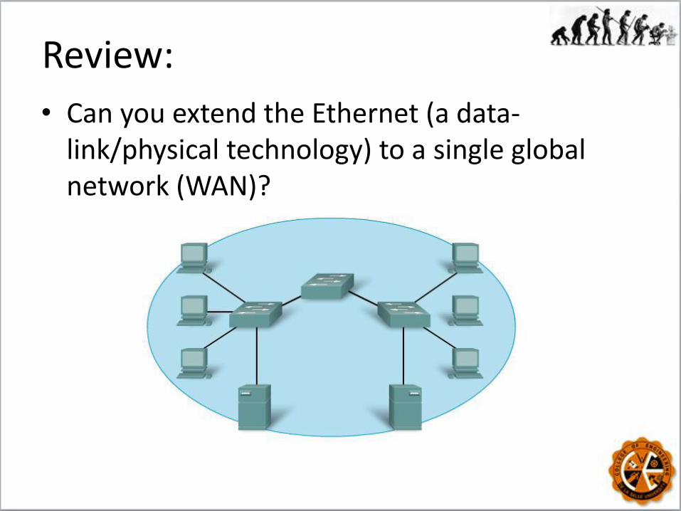
Review:
• Can you extend the Ethernet (a data-link/physical technology) to a single global network (WAN)?

Review:
• Why divide a network into smaller parts?

Understand • IP packets traverses unchanged via routers
from sub network to sub-network
Internet Protocol (IP) Concepts
• Delivery refers to the way a packet is handled by the underlying networks under the control of the network layer.
Ex. direct and indirect delivery
• Forwarding refers to the way a packet is delivered to the next station.
Delivery
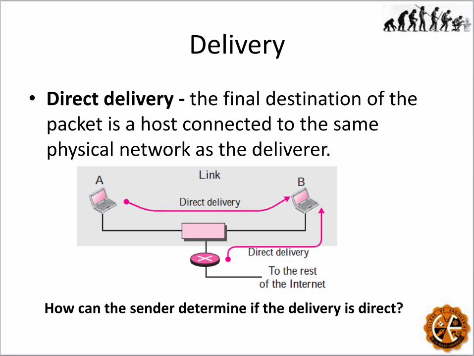
• Direct delivery - the final destination of the packet is a host connected to the same physical network as the deliverer.
How can the sender determine if the delivery is direct?

Delivery
• Indirect delivery - the packet goes from router to router until it reaches the one connected to the same physical network as its final destination.
Forwarding
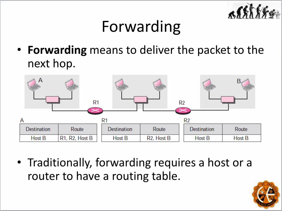
• Forwarding means to deliver the packet to the next hop.
• Traditionally, forwarding requires a host or a router to have a routing table.

Forwarding Techniques
• Next-hop method - the routing table holds only the address of the next hop instead of information about the complete route.
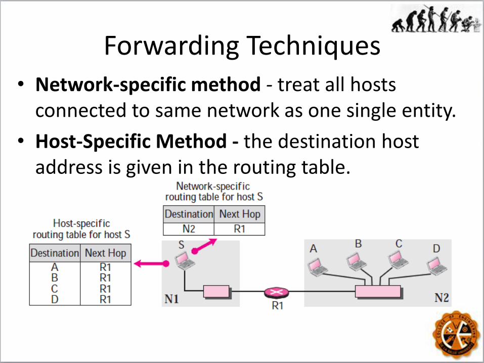
Forwarding Techniques • Network-specific method - treat all hosts
connected to same network as one single entity.
• Host-Specific Method - the destination host address is given in the routing table.

Forwarding Techniques
• Host-specific routing is used for purposes such as checking the route or providing security measures.
Forwarding Techniques
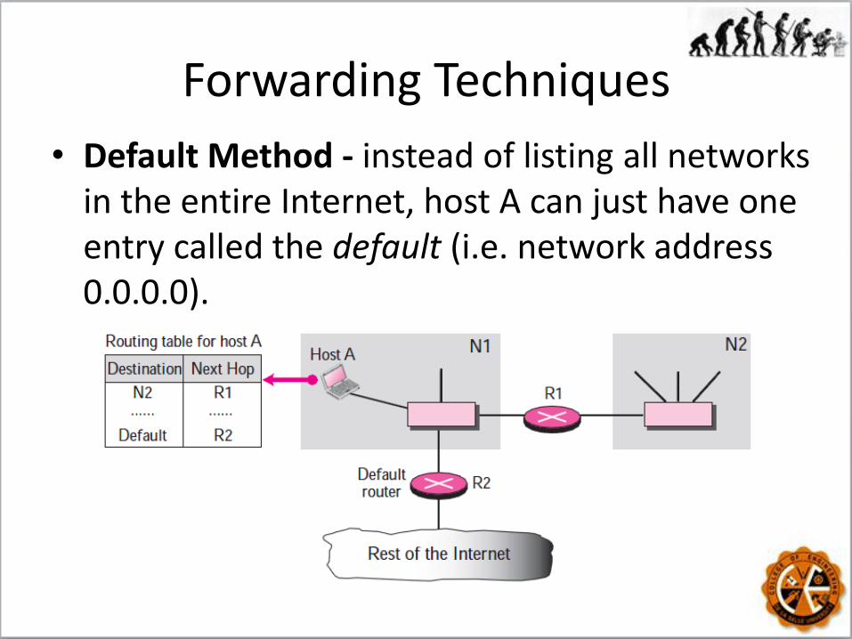
• Default Method - instead of listing all networks in the entire Internet, host A can just have one entry called the default (i.e. network address 0.0.0.0).

Forwarding with Classful Addressing
• Existence of a default mask in a classful address makes the forwarding process simple.

Forwarding with Classful Addressing
1. The destination address of the packet is extracted.
2. A copy of the destination address is used to find the class of the address. This is done by shifting the copy of the address 28 bits to the right. The result is a 4-bit number between 0 and 15. If the result is
a. 0 to 7, the class is A.
b. 8 to 11, the class is B.
c. 12 or 13, the class is C
d. 14, the class is D.
e. 15, the class is E.

Forwarding with Classful Addressing
3. The result of Step 2 for class A, B, or C and the destination address are used to extract the network address.
4. The class of the address and the network address are used to find next-hop information.
5. The ARP module uses the next-hop address and the interface number to find the physical address of the next router.
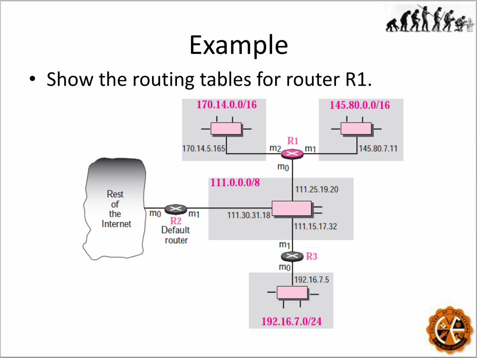
Example • Show the routing tables for router R1.

Solution • Some entries in the next-hop address column
are empty because in these cases, the destination is in the same network to which the router is connected (direct delivery).

Example • Router R1 in receives a packet with destination
address 192.16.7.14. Show how the packet is forwarded.
Solution • The destination address in binary is 11000000
00010000 00000111 00001110.
• A copy of the address is shifted 28 bits to the right. The result is 00000000 00000000 00000000 00001100 or 12. The destination network is class C.
• The network address is extracted by masking off the leftmost 24 bits of the destination address; the result is 192.16.7.0.
Solution
• The table for Class C is searched.
• The network address is found in the first row. The next-hop address 111.15.17.32. and the interface m0 are passed to ARP.
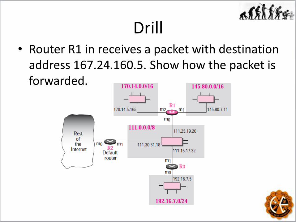
Drill • Router R1 in receives a packet with destination
address 167.24.160.5. Show how the packet is forwarded.
Solution • The destination address in binary is 10100111
00011000 10100000 00000101.
• A copy of the address is shifted 28 bits to the right. The result is 00000000 00000000 00000000 00001010 or 10. The class is B.
• The network address can be found by masking off 16 bits of the destination address, the result is 167.24.0.0. The table for Class B is searched.

Solution • No matching network address is found. The
packet needs to be forwarded to the default router.
• The next-hop address 111.30.31.18 and the interface number m0 are passed to ARP.
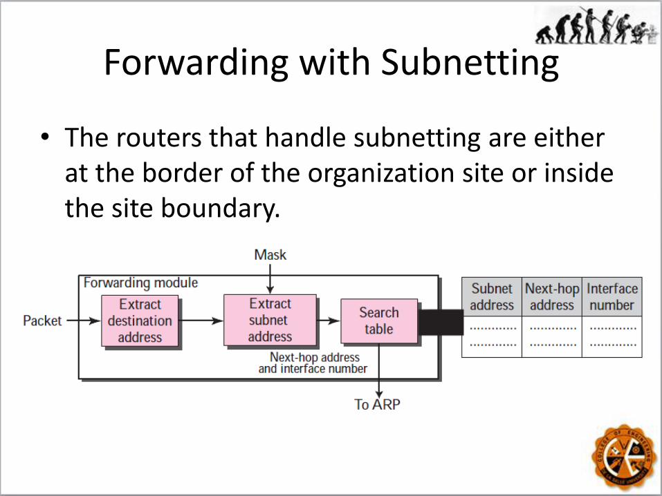
Forwarding with Subnetting
• The routers that handle subnetting are either at the border of the organization site or inside the site boundary.

Forwarding with Subnetting
1. The module extracts the destination address of the packet.
2. If the destination address matches any of the host-specific addresses in the table, the next-hop and the interface number is extracted from the table.
3. The destination address and the mask are used to extract the subnet address.
Forwarding with Subnetting
4. The table is searched using the subnet address to find the next-hop address and the interface number. If no match is found, the default is used.
5. The next-hop address and the interface number are given to ARP.
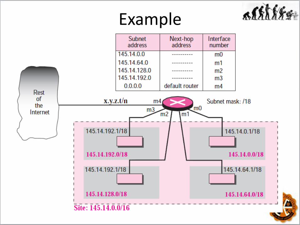
Example

Example • The site address is 145.14.0.0/16 (a class B).
• Every packet with destination address in the range 145.14.0.0 to 145.14.255.255 is delivered to the interface m4 and distributed to the final destination subnet by the router.
• x.y.z.t/n for the interface m4 because we do not know to which network this router is connected.
• The table has a default entry for packets that are to be sent out of the site.

Drill
• The router in previous figure receives a packet with destination address 145.14.32.78. Show how the packet is forwarded.
• Answer:
The mask is /18. After applying the mask, the subnet address is 145.14.0.0. The packet is delivered to ARP with the next-hop address 145.14.32.78 and the outgoing interface m0.
Drill
• The router in previous figure has a packet to send to the host with address 7.22.67.91. Show how the packet is routed.
• Answer:
The router receives the packet and applies the mask (/18). The network address is 7.22.64.0. The table is searched and the address is not found. The router uses the address of the default router and sends the packet to that router.

Forwarding with Classless Addressing
• In classless addressing, the whole address space is one entity; there are no classes.
• Thus, forwarding requires one row of information for each block involved.
• In classful addressing we can have a routing table with three columns;
• In classless addressing, we need at least four columns.
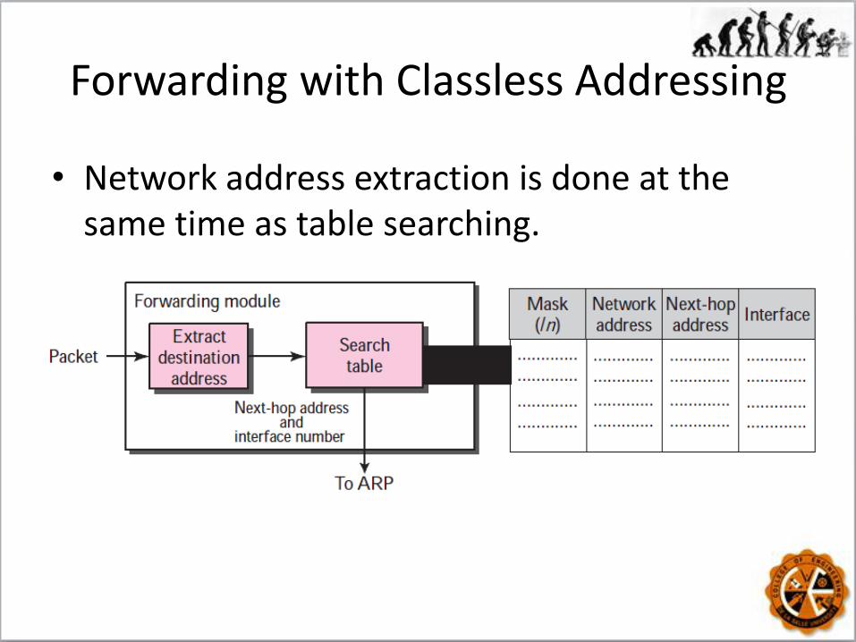
Forwarding with Classless Addressing
• Network address extraction is done at the same time as table searching.

Example
• Make a routing table for router R1 using the configuration.
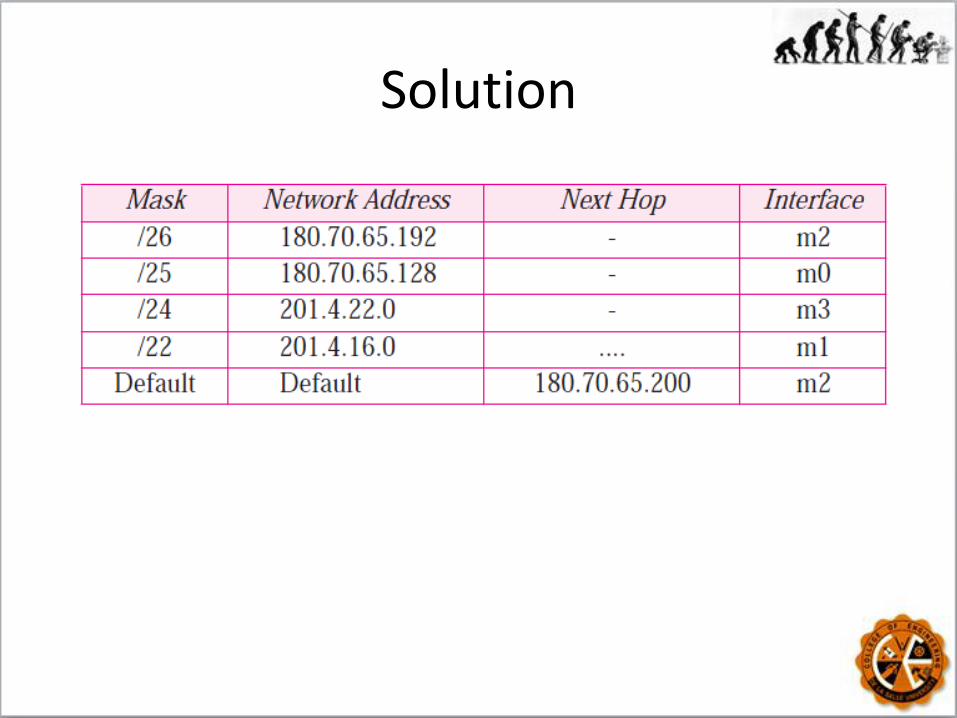
Solution
Example
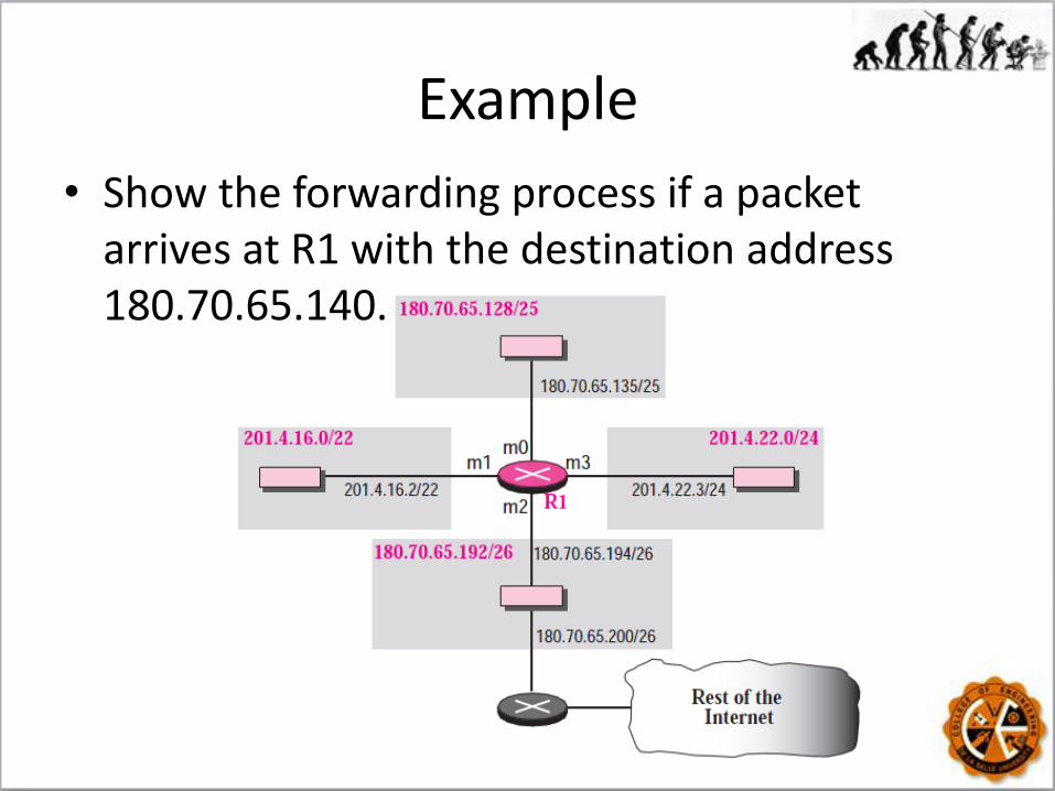
• Show the forwarding process if a packet arrives at R1 with the destination address 180.70.65.140.
Solution
• The first mask (/26) is applied to the destination address. The result is 180.70.65.128, which does not match the corresponding network address.
• The second mask (/25) is applied to the destination address. The result is 180.70.65.128, which matches the corresponding network address.
• The next-hop address and the interface number m0 are passed to ARP.
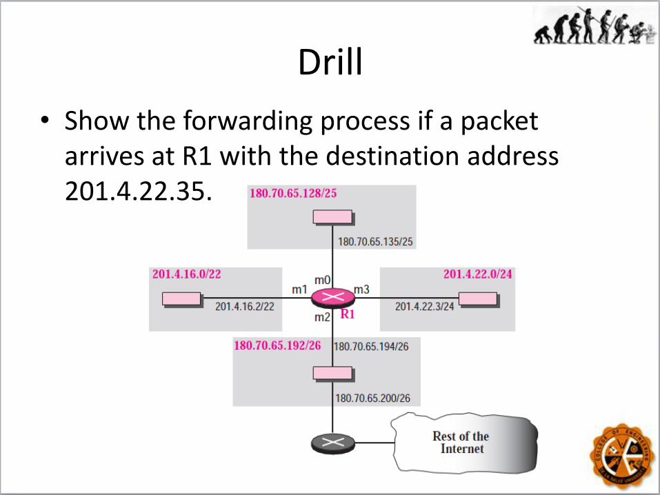
Drill
• Show the forwarding process if a packet arrives at R1 with the destination address 201.4.22.35.
Solution 1. The first mask (/26) is applied to the destination address. The result is 201.4.22.0, which does not match the corresponding network address (row 1).
2. The second mask (/25) is applied to the destination address. The result is 201.4.22.0, which does not match the corresponding network address (row 2).
3. The third mask (/24) is applied to the destination address. The result is 201.4.22.0, which matches the corresponding network address. The destination address of the packet and the interface number m3 are passed to ARP.

Example • Can we find the configuration of a router, R1,
if we know only its routing table?

What do we know?
• Three networks directly connected to router.
• Two networks indirectly connected to router.
• The router has three interfaces: m0, m1, & m2.
• There must be at least three other routers involved.
• One router, the default router, is connected to the rest of the Internet.
• But, we don’t know the …
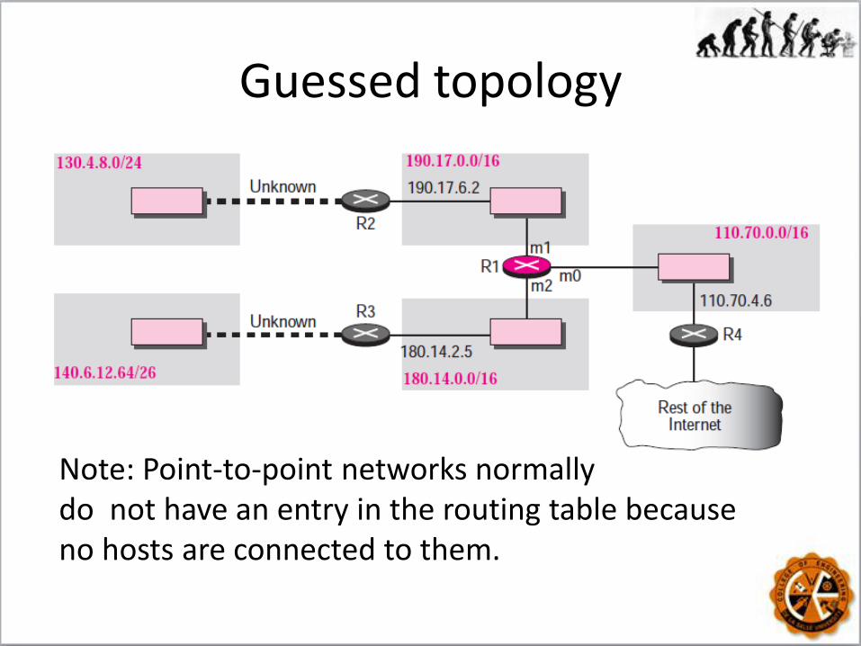
Guessed topology
Note: Point-to-point networks normally do not have an entry in the routing table because no hosts are connected to them.

Windows Routing Table
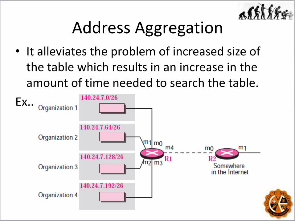
Address Aggregation • It alleviates the problem of increased size of
the table which results in an increase in the amount of time needed to search the table.
Ex..
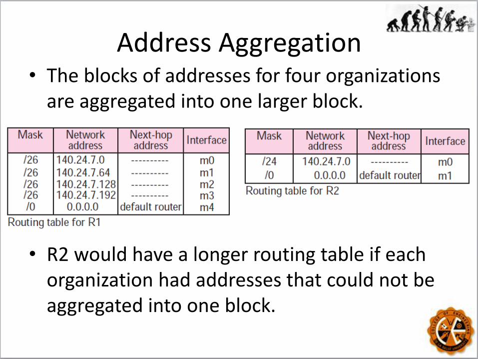
Address Aggregation • The blocks of addresses for four organizations
are aggregated into one larger block.
• R2 would have a longer routing table if each organization had addresses that could not be aggregated into one block.
Drill
• What happens if one of the organizations in the previous example is not geographically close to the other three?
• For example, if organization 4 cannot be connected to router R1 for some reason, can we still use the idea of address aggregation and still assign block 140.24.7.192/26 to organization 4?

Answer
• Yes because routing in classless addressing uses another principle, longest mask matching which states that the routing table is sorted from the longest mask to the shortest mask.
• Ex. Let there be three masks, /27, /26, and /24, the mask /27 must be the first entry and /24 must be last.

Longest mask matching
Hierarchical Routing
• To solve the problem of gigantic routing tables, we can create a sense of hierarchy in the routing tables.
• Ex. A local ISP can be assigned a single, but large, block of addresses with a certain prefix length. The local ISP can divide this block into smaller blocks of different sizes, and assign these to individual users and organizations, both large and small.
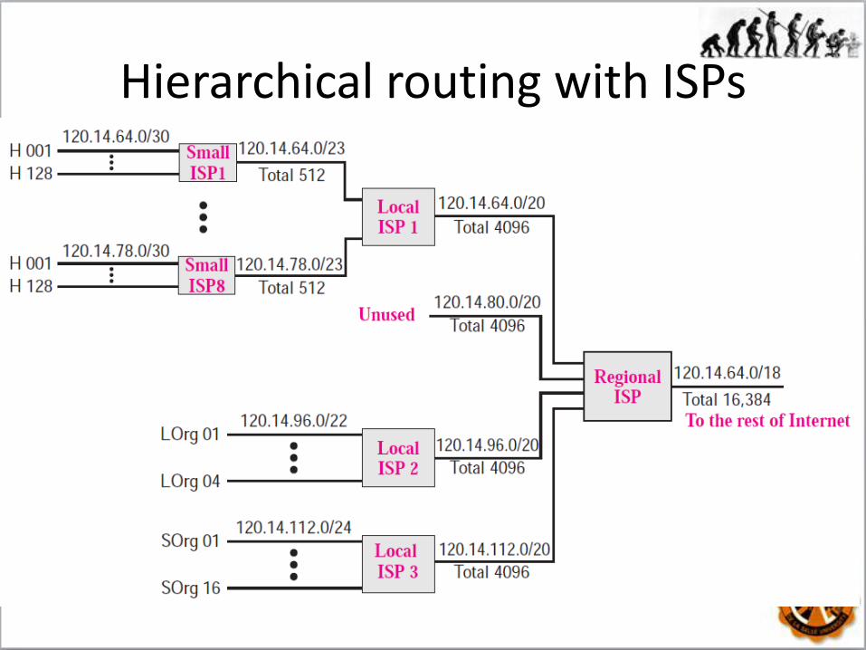
Hierarchical routing with ISPs

Geographical Routing
• To decrease the size of the routing table even further, we need to extend hierarchical routing to include geographical routing.
• We assign a block to America, a block to Europe, a block to Asia, a block to Africa, and so on.
• The routers of ISPs outside of Asia will have only one entry for packets to Asia in their routing tables.
Routing Table Search Algorithms
• In classful addressing, the routing table is organized as a list, divided into three tables (sometimes called buckets), one for each class.
• In classless addressing, there is no network information in the destination address. The simplest, but not the most efficient, search method is called the longest prefix match.

Forwarding Based on Destination Address and Label
• A connectionless network (datagram approach), a router forwards a packet based on the destination address in the header of packet.
• A connection-oriented network (virtual-circuit approach), a switch forwards a packet based on the label attached to a packet.

Forwarding based on destination address
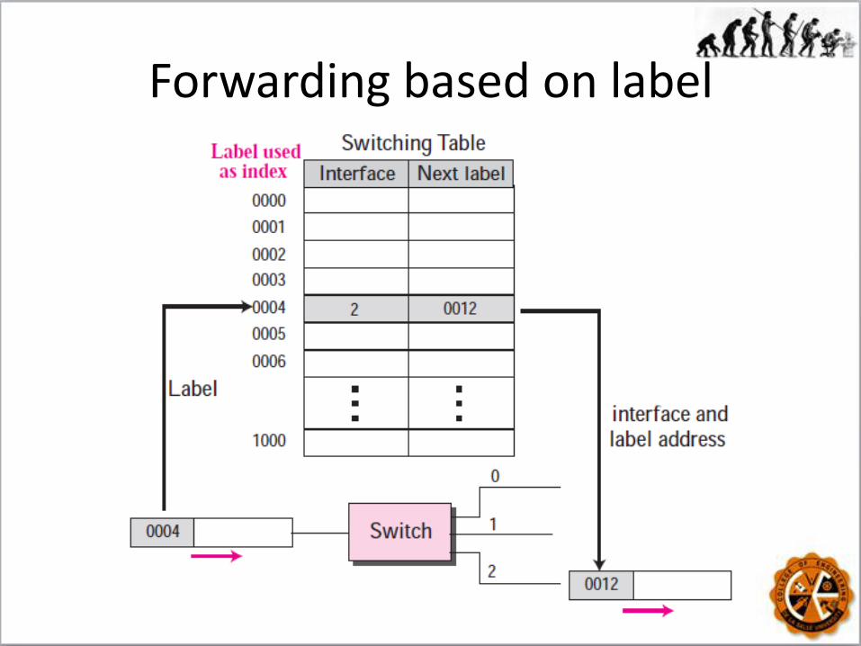
Forwarding based on label
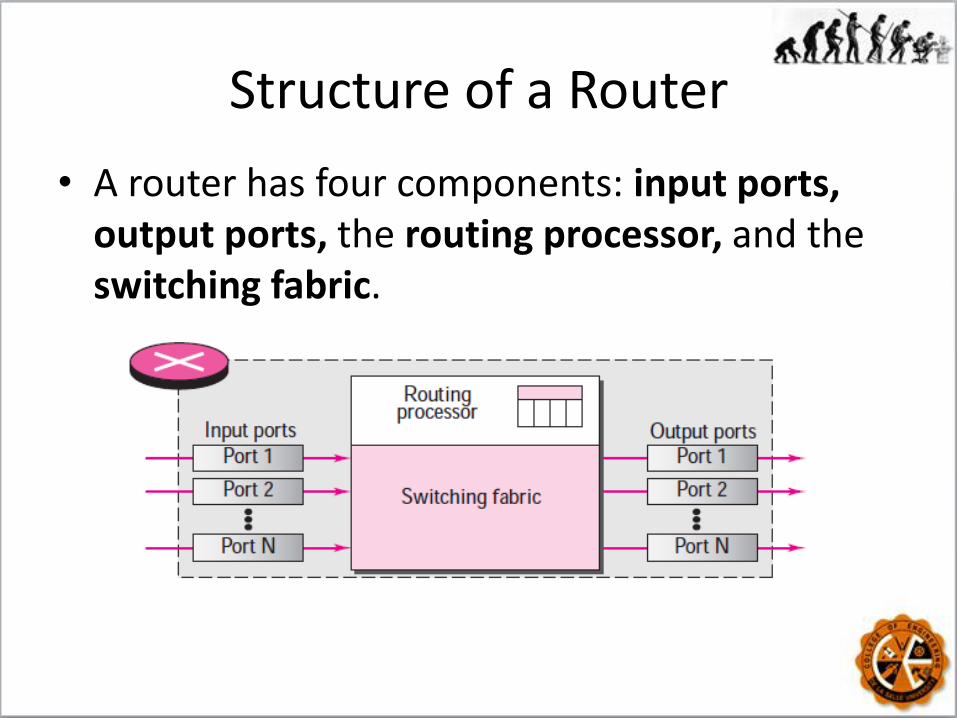
Structure of a Router
• A router has four components: input ports, output ports, the routing processor, and the switching fabric.
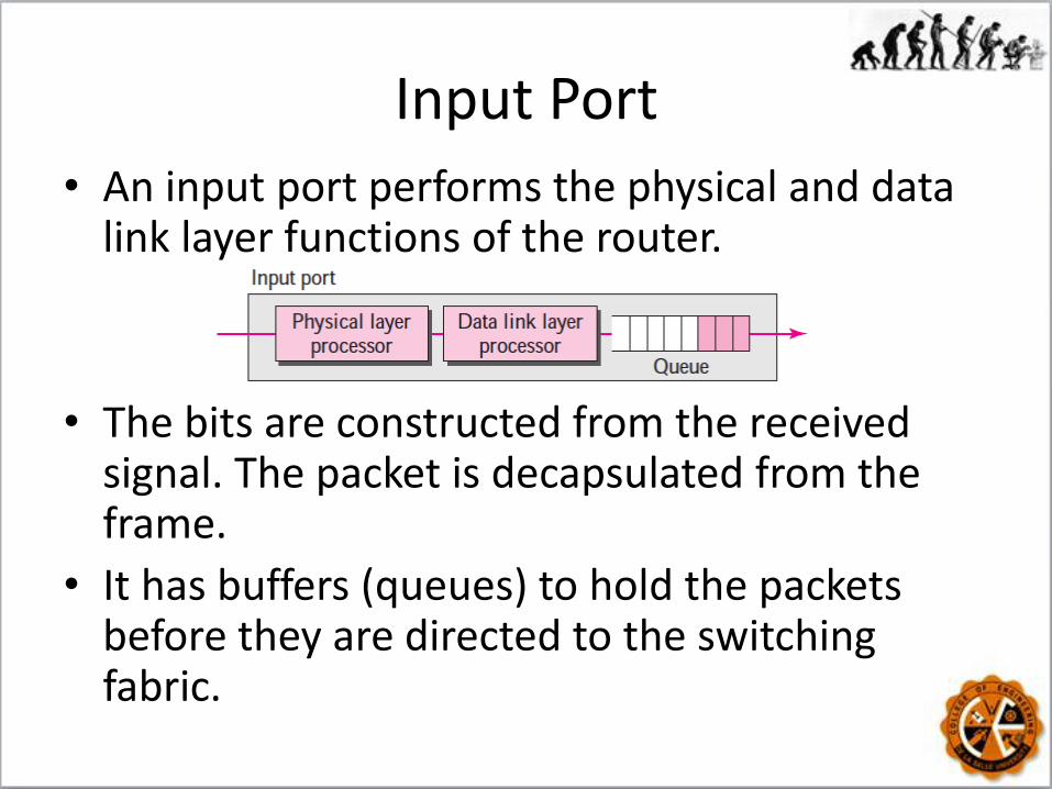
Input Port
• An input port performs the physical and data link layer functions of the router.
• The bits are constructed from the received signal. The packet is decapsulated from the frame.
• It has buffers (queues) to hold the packets before they are directed to the switching fabric.
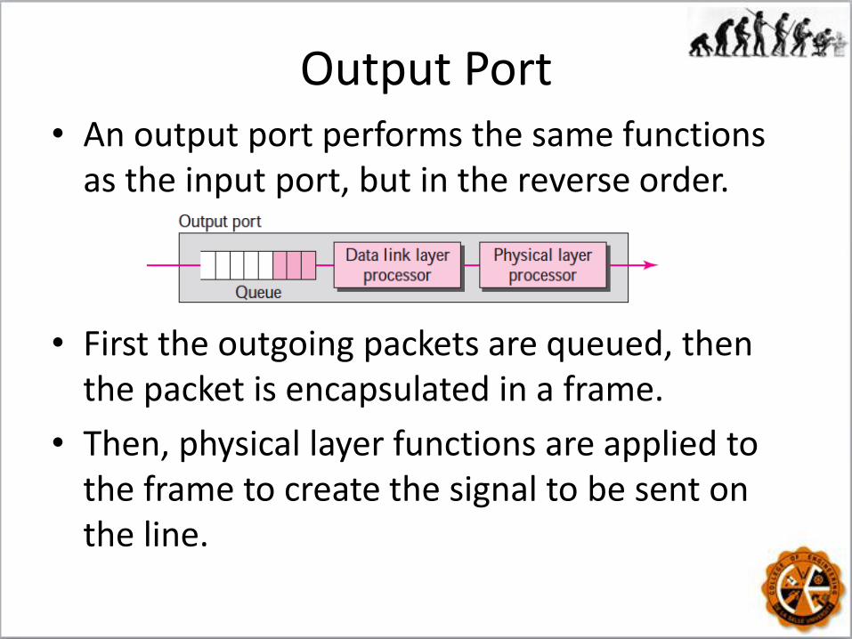
Output Port • An output port performs the same functions
as the input port, but in the reverse order.
• First the outgoing packets are queued, then the packet is encapsulated in a frame.
• Then, physical layer functions are applied to the frame to create the signal to be sent on the line.
Routing Processor
• The routing processor performs the functions of the network layer.
• The destination address is used to find the address of the next hop and, at the same time, the output port number from which the packet is sent out.
• This activity is sometimes referred to as table lookup because the routing processor searches the routing table.

Switching Fabrics
• Switching fabrics move the packet from the input queue to the output queue.
• The simplest type of switching fabric is the crossbar switch:
A crossbar switch connects n inputs to n outputs in a grid, using electronic microswitches at each crosspoint.

Switching Fabrics • A banyan switch is a multistage switch with
microswitches at each stage that route the packets based on the output port represented as a binary string.

Router Functions
• Connect LANs to make an internetwork

Router Functions
• Routers interconnect LANs to form the Internet
In Summary
• Routers connect LANs, and switches connect computers.
• Routers work with logical (IP) addresses rather than physical (MAC) addresses, as switches do.
• Routers work with packets rather than the frames that switches work with.
• Routers don’t forward broadcast packets, but switches do.
• Routers use routing tables, and switches use switching tables.
Datagram
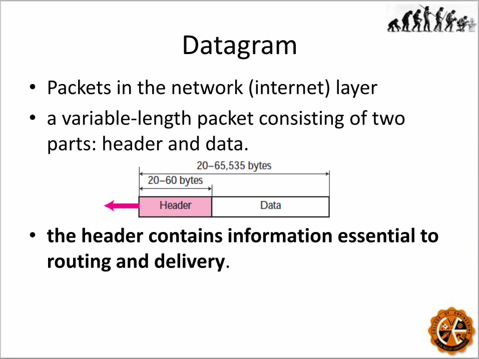
• Packets in the network (internet) layer
• a variable-length packet consisting of two parts: header and data.
• the header contains information essential to routing and delivery.

IP Header Format
IP Header Contents
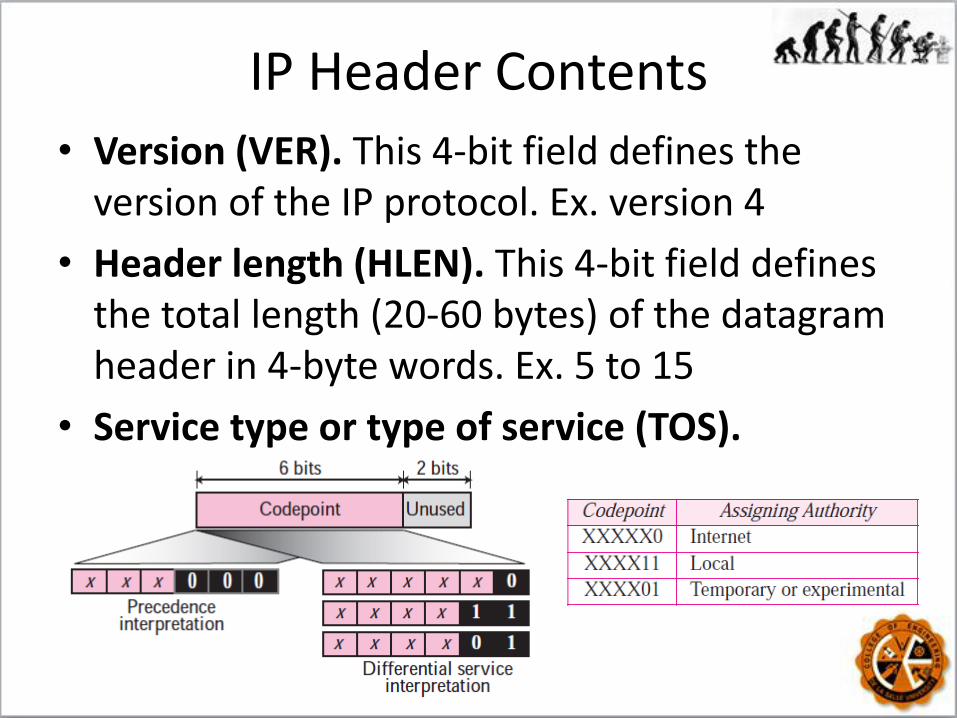
• Version (VER). This 4-bit field defines the version of the IP protocol. Ex. version 4
• Header length (HLEN). This 4-bit field defines the total length (20-60 bytes) of the datagram header in 4-byte words. Ex. 5 to 15
• Service type or type of service (TOS).

IP Header Contents
• Total length. This is a 16-bit field that defines the total length (header plus data) of the IP datagram in bytes.
Length of data = total length − header length
• Thus, the total length of the IP datagram is limited to:
65,535 (216 − 1) bytes
IP Header Contents
• Identification, Flags, and Fragmentation offset. used in fragmentation
• Time to live. used to control the maximum number of hops (routers) visited by the datagram.
What if the source wants to confine the packet
to the local network?

IP Header Contents • Protocol. This 8-bit field defines the higher-
level protocol that uses services of the IP layer.
• An IP datagram can encapsulate data from several higher level protocols such as TCP, UDP, ICMP, and IGMP.

IP Header Contents
• Source address. This 32-bit field defines the IP address of the source.
• Destination address. This 32-bit field defines the IP address of the destination.
• Checksum. Error detection. It is formed by adding bit streams using one’s complement arithmetic and then complementing the result.
Drill
• An IP packet has arrived with the first 8 bits as shown:
01000010
Will the receiver accept or discard the packet? Why?

Drill
• An IP packet has arrived with the first few hexadecimal digits as shown below:
45000028000100000102 . . .
• How many hops can this packet travel before being dropped?
• The data belong to what upper layer protocol?

Fragmentation • The division of a packet into smaller units to
accommodate a protocol’s MTU.
• Maximum transfer unit (MTU) The largest size data unit a specific network can handle.
• Ex. Ethernet LAN = 1500 bytes,
FDDI LAN = 4352 bytes, PPP = 296 bytes, etc.
Fragmentation
• In order to make the IP protocol independent of the physical network, the maximum length of the IP datagram was set to 65,535 bytes.
• Thus, for other physical networks, we must divide the datagram to make it possible to pass through these networks.
• Only data in a datagram is fragmented.
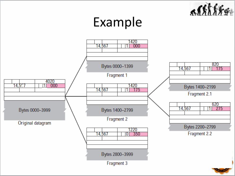
Example
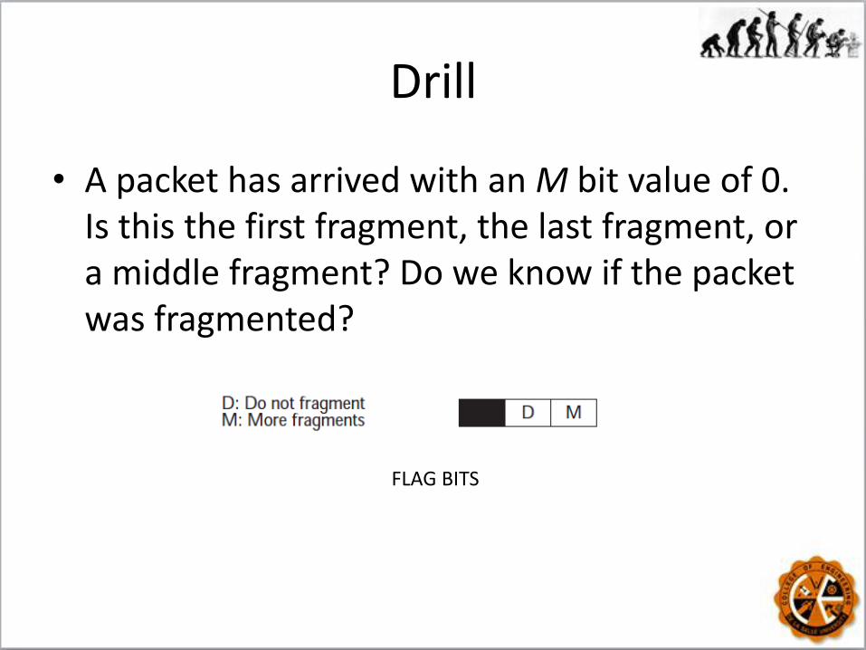
Drill
• A packet has arrived with an M bit value of 0. Is this the first fragment, the last fragment, or a middle fragment? Do we know if the packet was fragmented?
FLAG BITS
Drill
• A packet has arrived with an M bit value of 1. Is this the first fragment, the last fragment, or a middle fragment? Do we know if the packet was fragmented?

Drill
• A packet has arrived with an M bit value of 1 and a fragmentation offset value of zero. Is this the first fragment, the last fragment, or a middle fragment?
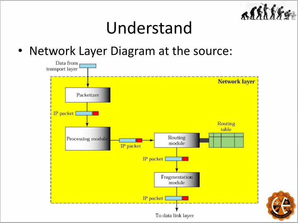
Understand • Network Layer Diagram at the source:
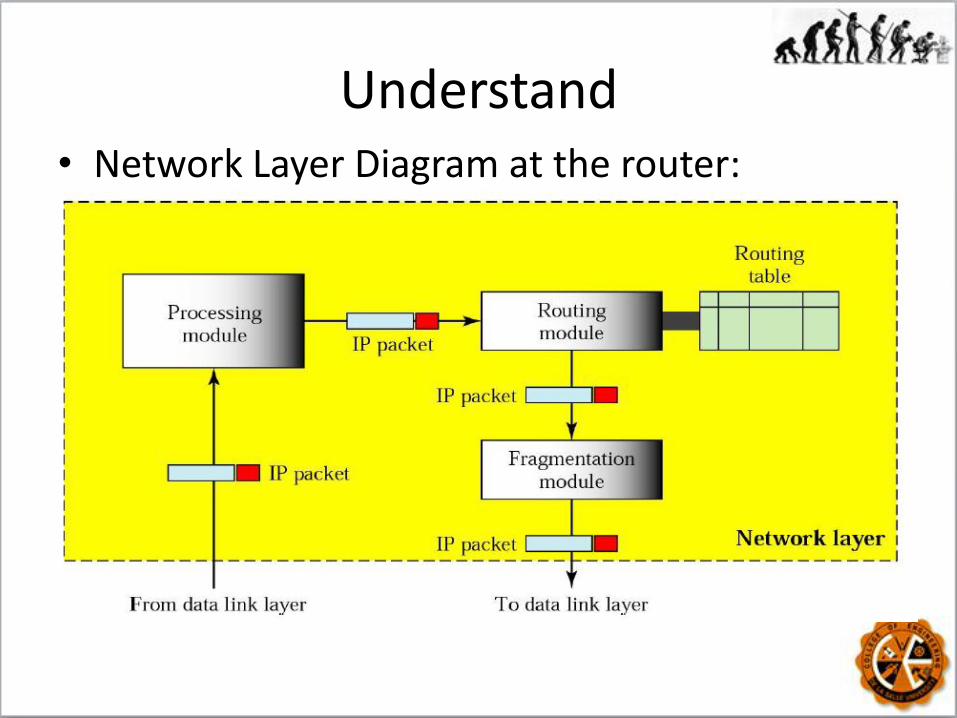
Understand • Network Layer Diagram at the router:

Understand
• Network Layer Diagram at the destination:
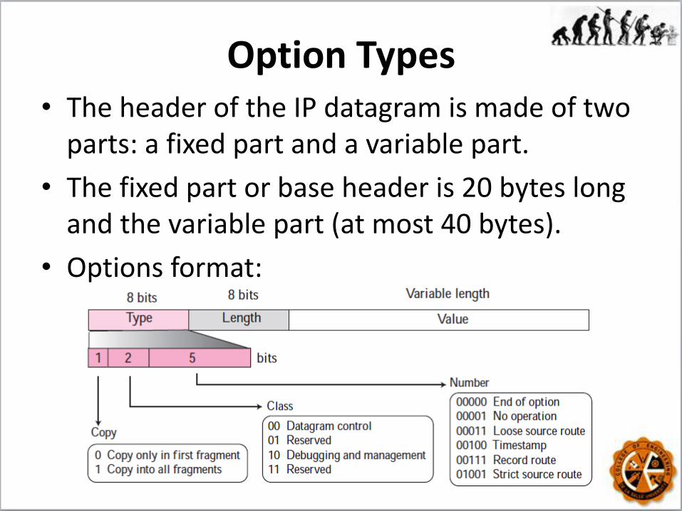
Option Types • The header of the IP datagram is made of two
parts: a fixed part and a variable part.
• The fixed part or base header is 20 bytes long and the variable part (at most 40 bytes).
• Options format:
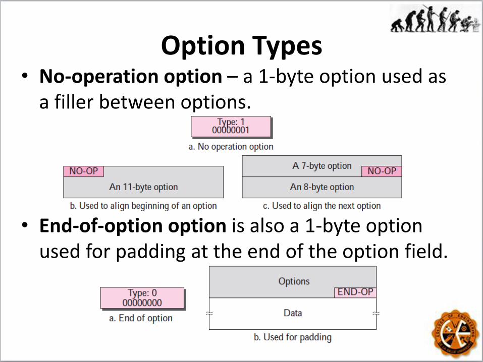
Option Types • No-operation option – a 1-byte option used as
a filler between options.
• End-of-option option is also a 1-byte option used for padding at the end of the option field.

• Record-route option - used to record the Internet routers that handle the datagram.
* Pointer points to the first available entry.
*

• Strict-source-route option is used by the source to predetermine a route for the datagram as it travels through the Internet.
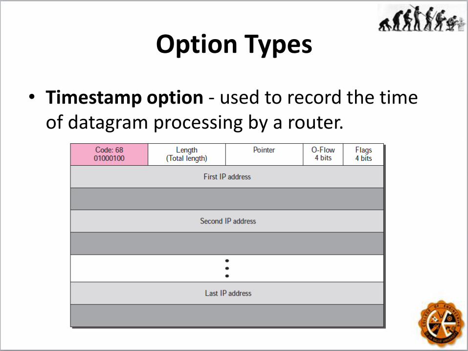
Option Types
• Timestamp option - used to record the time of datagram processing by a router.

Drill
• Which of the six options must be copied to each fragment?
a. No operation
b. End of option
c. Record route
d. Strict source route
e. Loose source route
f. Timestamp
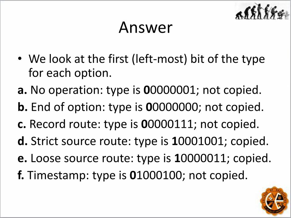
Answer
• We look at the first (left-most) bit of the type for each option.
a. No operation: type is 00000001; not copied.
b. End of option: type is 00000000; not copied.
c. Record route: type is 00000111; not copied.
d. Strict source route: type is 10001001; copied.
e. Loose source route: type is 10000011; copied.
f. Timestamp: type is 01000100; not copied.
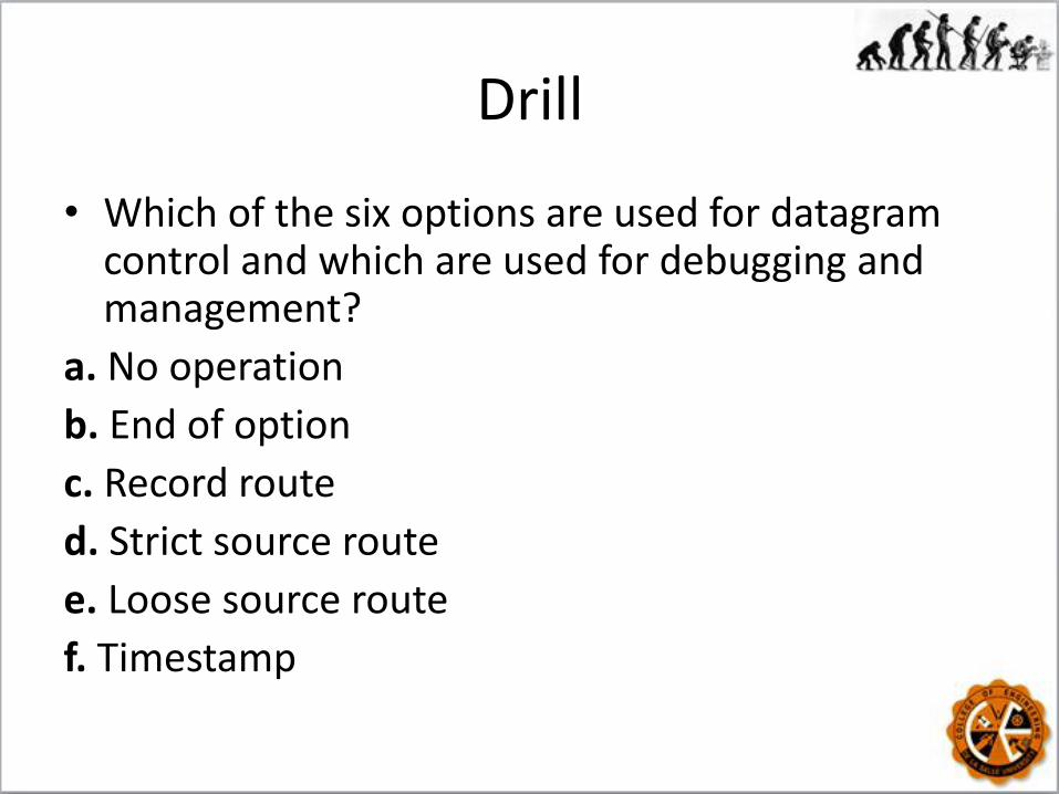
Drill
• Which of the six options are used for datagram control and which are used for debugging and management?
a. No operation
b. End of option
c. Record route
d. Strict source route
e. Loose source route
f. Timestamp

Answer
• We look at the second and third (left-most) bits of the type.
a. No operation: type is 00000001; datagram control. b. End of option: type is 00000000; datagram control. c. Record route: type is 00000111; datagram control. d. Strict source route: type is 10001001; datagram control. e. Loose source route: type is 10000011; datagram control. f. Timestamp: type is 01000100; debugging and management control.
ping utility
• An application program to determine the reachability of a destination using an ICMP echo request and reply.
ping dlsu.edu.ph
• Use the ping utility with the -R option to implement the record route option and show the interfaces and IP addresses.
traceroute utility
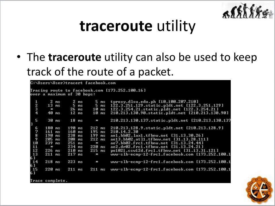
• The traceroute utility can also be used to keep track of the route of a packet.
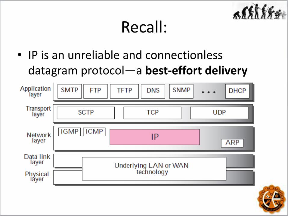
Recall:
• IP is an unreliable and connectionless datagram protocol—a best-effort delivery

ARP Revisited
• A protocol for obtaining the physical address of a node when the Internet address is known.
• Position of ARP in TCP/IP protocol suite:
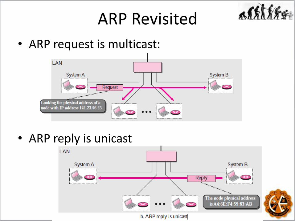
ARP Revisited
• ARP request is multicast:
• ARP reply is unicast

ARP Packet Format
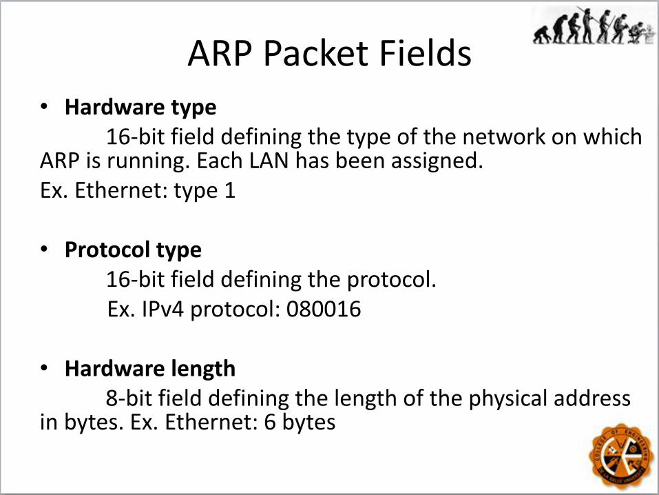
ARP Packet Fields • Hardware type 16-bit field defining the type of the network on which ARP is running. Each LAN has been assigned. Ex. Ethernet: type 1 • Protocol type 16-bit field defining the protocol. Ex. IPv4 protocol: 080016 • Hardware length 8-bit field defining the length of the physical address in bytes. Ex. Ethernet: 6 bytes
ARP Packet Fields
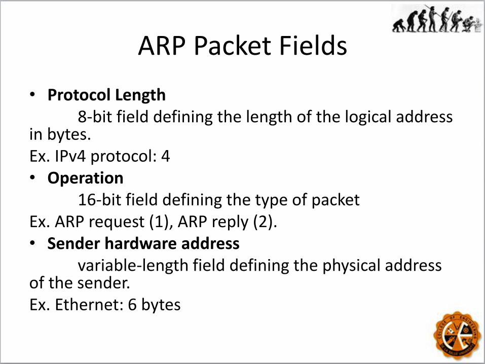
• Protocol Length 8-bit field defining the length of the logical address in bytes. Ex. IPv4 protocol: 4 • Operation 16-bit field defining the type of packet Ex. ARP request (1), ARP reply (2). • Sender hardware address variable-length field defining the physical address of the sender. Ex. Ethernet: 6 bytes

ARP Packet Fields
• Sender protocol address variable-length field defining the logical address of the sender. Ex. IPv4 protocol: 4 bytes • Target hardware address variable-length field defining the physical address of the target. Ex. Ethernet: 6 bytes • Target protocol address variable-length field defining the logical address of the target. Ex. IPv4 protocol: 4bytes
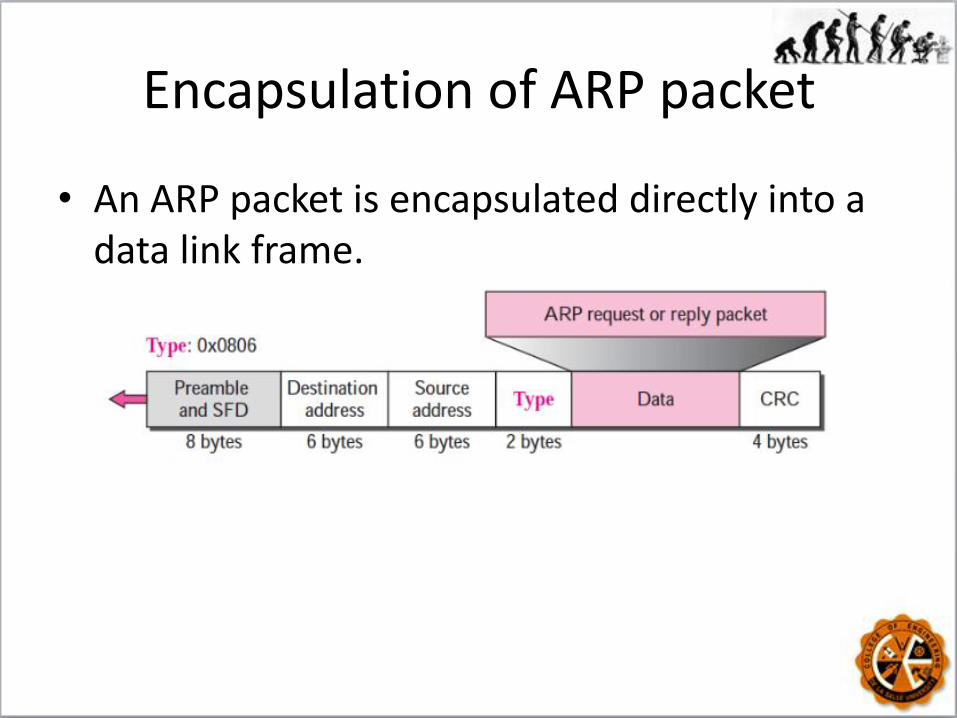
Encapsulation of ARP packet
• An ARP packet is encapsulated directly into a data link frame.
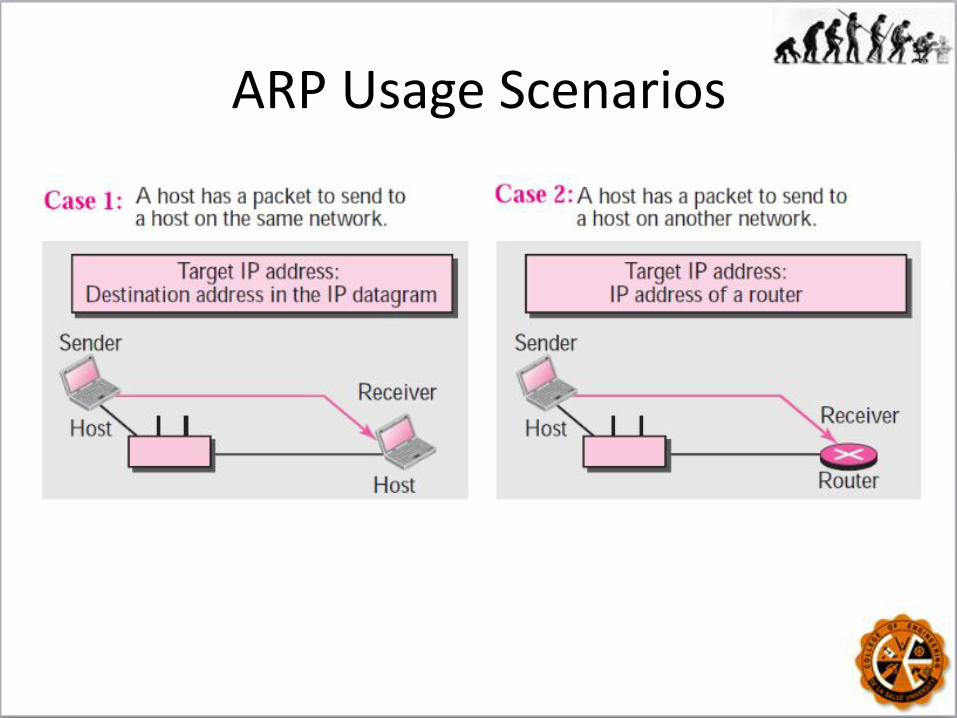
ARP Usage Scenarios

ARP Usage Scenarios
Example
A host with IP address 130.23.43.20 and physical address B2 : 34 : 55 : 10 : 22 : 10 has a packet to send to another host with IP address 130.23.43.25 and physical address A4 : 6E : F4 : 59 : 83 : AB (which is unknown to the first host). The two hosts are on the same Ethernet network. Show the ARP request and reply packets encapsulated in Ethernet frames.
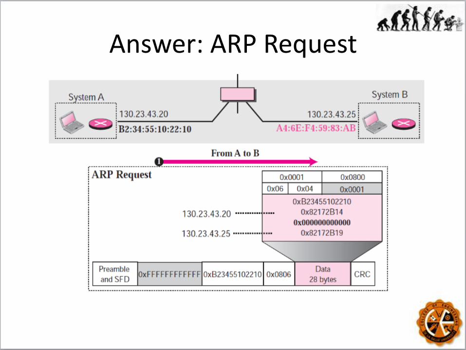
Answer: ARP Request
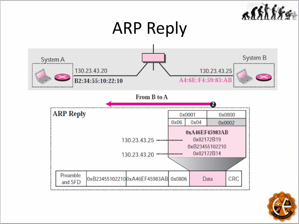
ARP Reply
ARP Package
• ARP package involves five components: a cache table, queues, an output module, an input module, and a cache-control module.
• The package receives an IP datagram that needs to be encapsulated in a frame that needs the destination physical (hardware) address.
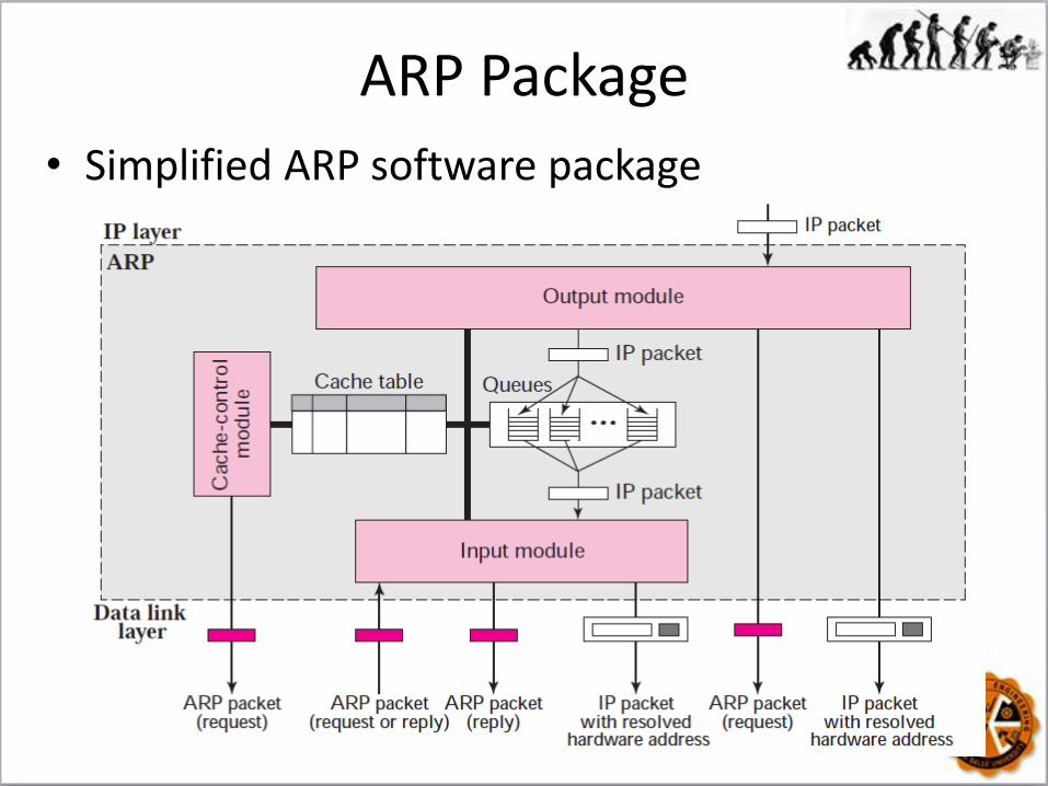
ARP Package
• Simplified ARP software package
ARP Components
• Cache Table - When a host or router receives the corresponding physical address for an IP datagram, the address can be saved in the cache table.
• The address can be used for the datagrams destined for the same receiver within the next few minutes.
• Cache Table is implemented as an array of entries.
Cache Table Entries
• State. This column shows the state of the entry. It can have one of three values:
FREE, PENDING, or RESOLVED.
- FREE state means that the time-to-live for this entry has expired.
- PENDING state means a request for this entry has been sent, but the reply has not yet been received.
- RESOLVED state means that the entry is complete. The entry now has the physical (hardware) address of the destination.
Cache Table Entries
• Hardware type, Protocol type, Hardware length, Protocol length. This columns is the same as the corresponding field in the ARP packet.
• Interface number. A router can be connected to different networks, each with a different interface number. Each network can have different hardware and protocol types.

Cache Table Entries
• Queue number. ARP uses numbered queues to enqueue the packets waiting for address resolution. Packets for the same destination are usually enqueued in the same queue.
• Attempts. This column shows the number of times an ARP request is sent out for this entry.
• Time-out. This column shows the lifetime of an entry in seconds.

Cache Table Entries
• Hardware address. This column shows the destination hardware address. It remains empty until resolved by an ARP reply.
• Protocol address. This column shows the destination IP address.
Queues
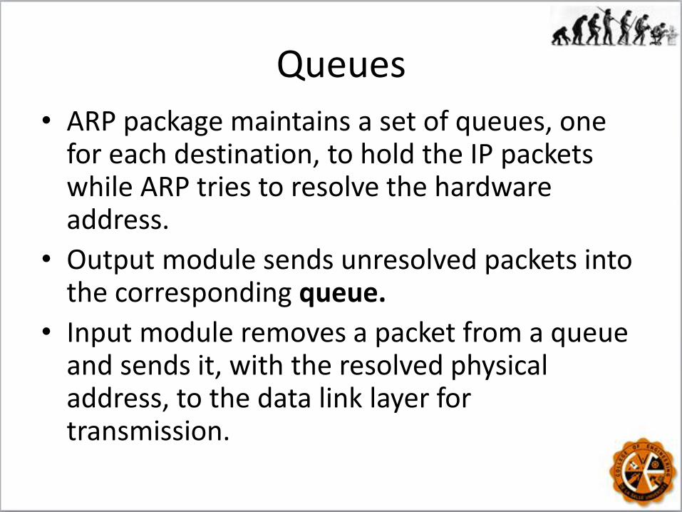
• ARP package maintains a set of queues, one for each destination, to hold the IP packets while ARP tries to resolve the hardware address.
• Output module sends unresolved packets into the corresponding queue.
• Input module removes a packet from a queue and sends it, with the resolved physical address, to the data link layer for transmission.
Output Module
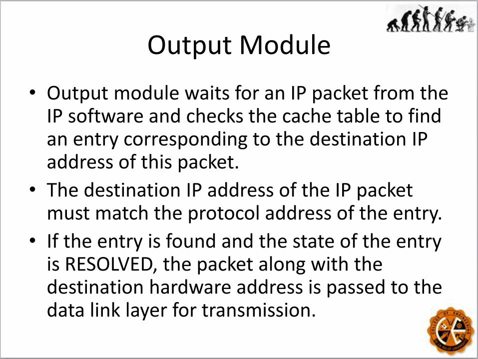
• Output module waits for an IP packet from the IP software and checks the cache table to find an entry corresponding to the destination IP address of this packet.
• The destination IP address of the IP packet must match the protocol address of the entry.
• If the entry is found and the state of the entry is RESOLVED, the packet along with the destination hardware address is passed to the data link layer for transmission.

Output Module
• If the entry is found and the state of the entry is PENDING, the packet waits until the destination hardware address is found.
• If no entry is found, the module creates a queue and enqueues the packet. A new entry with the state of PENDING is created for this destination and the value of the ATTEMPTS field is set to 1.
• An ARP request packet is then broadcast.
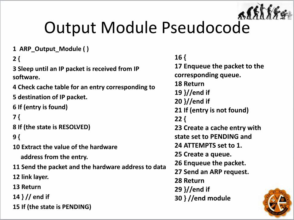
Output Module Pseudocode 1 ARP_Output_Module ( )
2 {
3 Sleep until an IP packet is received from IP software.
4 Check cache table for an entry corresponding to
5 destination of IP packet.
6 If (entry is found)
7 {
8 If (the state is RESOLVED)
9 {
10 Extract the value of the hardware
address from the entry.
11 Send the packet and the hardware address to data
12 link layer.
13 Return
14 } // end if
15 If (the state is PENDING)
16 { 17 Enqueue the packet to the corresponding queue. 18 Return 19 }//end if 20 }//end if 21 If (entry is not found) 22 { 23 Create a cache entry with state set to PENDING and 24 ATTEMPTS set to 1. 25 Create a queue. 26 Enqueue the packet. 27 Send an ARP request. 28 Return 29 }//end if 30 } //end module
Input Module
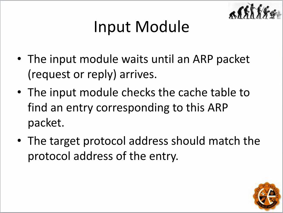
• The input module waits until an ARP packet (request or reply) arrives.
• The input module checks the cache table to find an entry corresponding to this ARP packet.
• The target protocol address should match the protocol address of the entry.

Input Module
• If the entry is found and the state of the entry is PENDING, the module updates the entry by copying the target hardware address in the packet to the hardware address field of the entry and changing the state to RESOLVED.
• If the entry is found and the state is RESOLVED, the module still updates the entry.
• This is because the target hardware address could have been changed.
Input Module
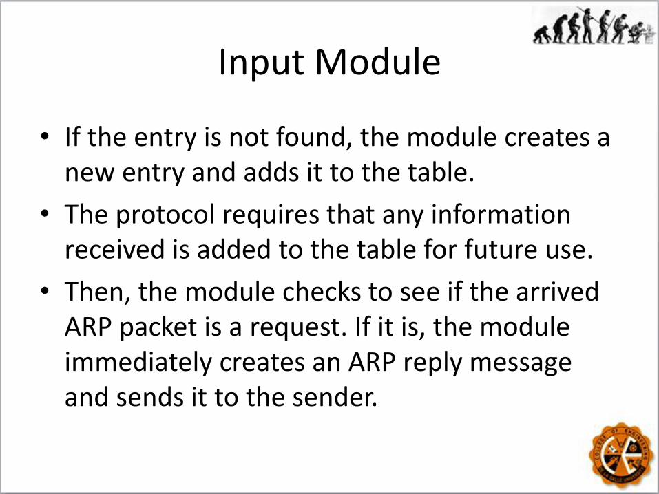
• If the entry is not found, the module creates a new entry and adds it to the table.
• The protocol requires that any information received is added to the table for future use.
• Then, the module checks to see if the arrived ARP packet is a request. If it is, the module immediately creates an ARP reply message and sends it to the sender.
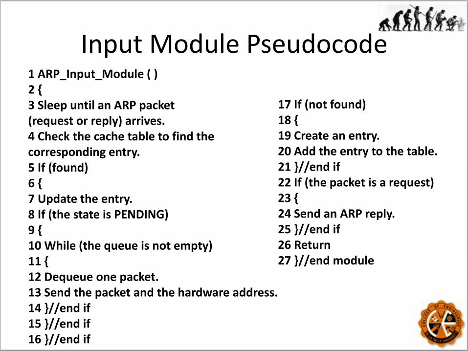
Input Module Pseudocode 1 ARP_Input_Module ( ) 2 { 3 Sleep until an ARP packet (request or reply) arrives. 4 Check the cache table to find the corresponding entry. 5 If (found) 6 { 7 Update the entry. 8 If (the state is PENDING) 9 { 10 While (the queue is not empty) 11 { 12 Dequeue one packet. 13 Send the packet and the hardware address. 14 }//end if 15 }//end if 16 }//end if
17 If (not found) 18 { 19 Create an entry. 20 Add the entry to the table. 21 }//end if 22 If (the packet is a request) 23 { 24 Send an ARP reply. 25 }//end if 26 Return 27 }//end module

Cache Module
• It periodically checks the cache table, entry by entry.
• If the state of the entry is FREE, it continues to the next entry.
• If the state is PENDING, the module increments the value of the attempts field by 1.
• If the state of the entry is RESOLVED, the module decrements the value of the time-out field by the amount of time elapsed since the last check.

Cache Module Pseudocode
1 ARP_Cache_Control_Module ( ) 2 { 3 Sleep until the periodic timer matures. 4 Repeat for every entry in the cache table 5 { 6 If (the state is FREE) 7 { 8 Continue. 9 }//end if 10 If (the state is PENDING) 11 {

Cache Module Pseudocode
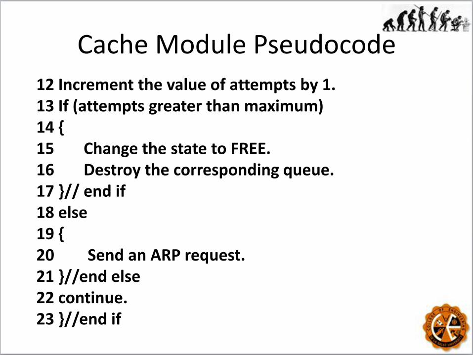
12 Increment the value of attempts by 1. 13 If (attempts greater than maximum) 14 { 15 Change the state to FREE. 16 Destroy the corresponding queue. 17 }// end if 18 else 19 { 20 Send an ARP request. 21 }//end else 22 continue. 23 }//end if
Cache Module Pseudocode
12 Increment the value of attempts by 1. 13 If (attempts greater than maximum) 14 { 15 Change the state to FREE. 16 Destroy the corresponding queue. 17 }// end if 18 else 19 { 20 Send an ARP request. 21 }//end else 22 continue. 23 }//end if

Cache Module Pseudocode
24 If (the state is RESOLVED) 25 { 26 Decrement the value of time-out. 27 If (time-out less than or equal 0) 28 { 29 Change the state to FREE. 30 Destroy the corresponding queue. 31 }//end if 32 }//end if 33 }//end repeat 34 Return. 35 }//end module
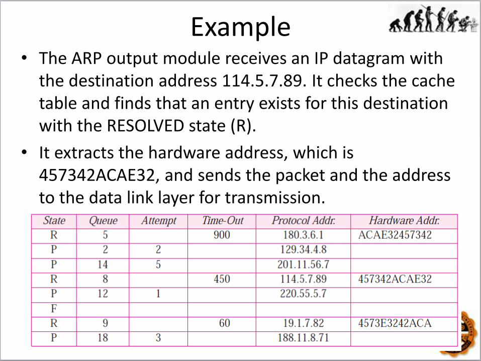
Example • The ARP output module receives an IP datagram with
the destination address 114.5.7.89. It checks the cache table and finds that an entry exists for this destination with the RESOLVED state (R).
• It extracts the hardware address, which is 457342ACAE32, and sends the packet and the address to the data link layer for transmission.

Drill • Twenty seconds later, the ARP output module receives
an IP datagram (from the IP layer) with the destination address 116.1.7.22.
Answer
• It checks the cache table and does not find this destination in the table.
• The module adds an entry to the table with the state PENDING and the Attempt value 1.
• It creates a new queue for this destination and enqueues the packet.
• It then sends an ARP request to the data link layer for this destination.

Answer
RARP
• Reverse Address Resolution Protocol (RARP)-
a version of ARP designed to provide the IP address for a booted computer.
• ARP maps an IP address to a physical address: RARP maps a physical address to an IP address.
• RARP used the broadcast service of the data link layer, which means that a RARP server must be present in each network.
• RARP can provide only the IP address of the computer
Routing Protocols
• Routing protocols have been created in response to the demand for dynamic routing tables.
• A routing protocol is a combination of rules and procedures that lets routers in the internet inform each other of changes.
• Ex. The sharing of information allows a router in Greenhills to know about the failure of a network in Paranaque.
Intra- and Inter-Domain Routing
• Routing inside an autonomous system is referred to as intra-domain routing.
• Routing between autonomous systems is referred to as inter-domain routing.
• Note: An autonomous system (AS) is a group of networks and routers under the authority of a single administration.

Autonomous system (AS)

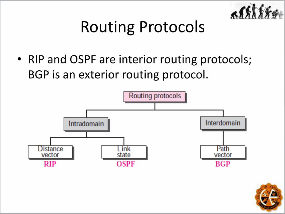
Routing Protocols
• Unicast Routing Protocols:
- Routing Information Protocol (RIP) - based on the distance vector routing algorithm.
- Open shortest path first (OSPF) - interior
routing protocol based on link state routing.
- Border Gateway Protocol (BGP) - interautonomous system routing protocol based on path vector routing.
• Multicasting and Multicast Routing Protocols
Routing Protocols
• RIP and OSPF are interior routing protocols; BGP is an exterior routing protocol.
Distance Vector Routing
• This method sees an AS, with all routers and networks, as a graph, a set of nodes and lines (edges) connecting the nodes.
• The graph theory used an algorithm called Bellman-Ford (also called Ford-Fulkerson) for a while to find the shortest path between nodes in a graph given the distance between nodes.
Bellman-Ford Algorithm
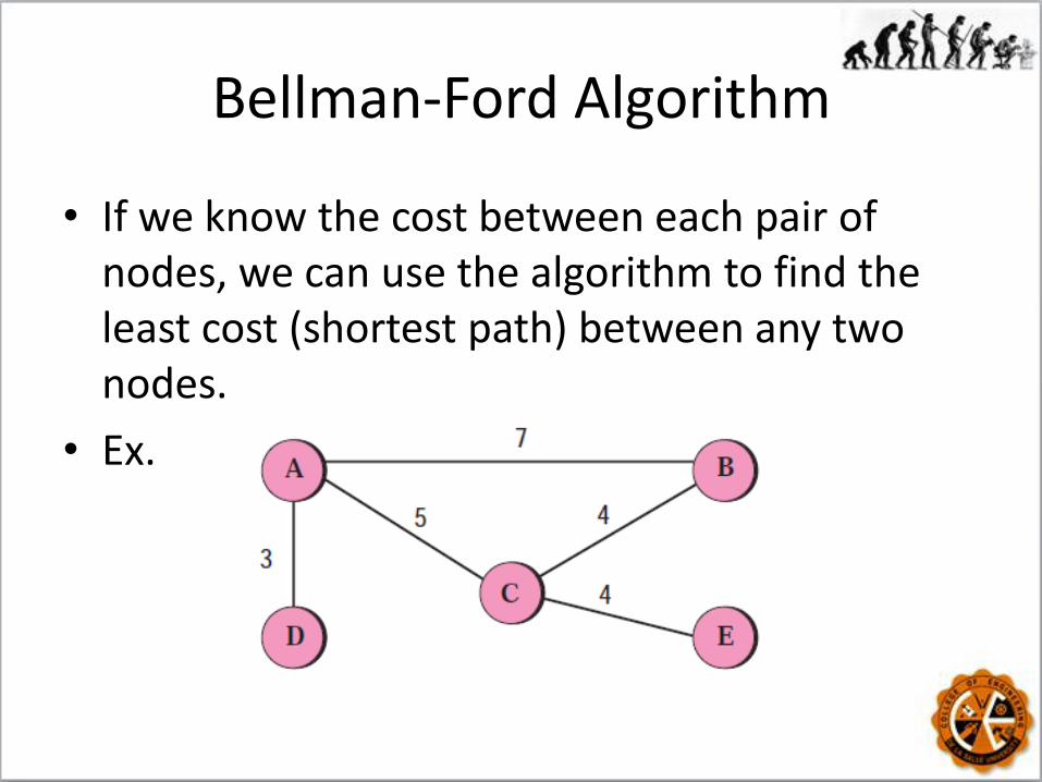
• If we know the cost between each pair of nodes, we can use the algorithm to find the least cost (shortest path) between any two nodes.
• Ex.
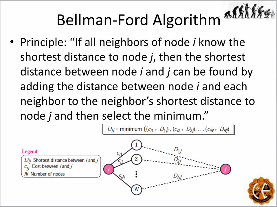
Bellman-Ford Algorithm • Principle: “If all neighbors of node i know the
shortest distance to node j, then the shortest distance between node i and j can be found by adding the distance between node i and each neighbor to the neighbor’s shortest distance to node j and then select the minimum.”
Bellman-Ford Algorithm
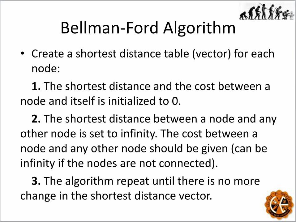
• Create a shortest distance table (vector) for each node:
1. The shortest distance and the cost between a node and itself is initialized to 0.
2. The shortest distance between a node and any other node is set to infinity. The cost between a node and any other node should be given (can be infinity if the nodes are not connected).
3. The algorithm repeat until there is no more change in the shortest distance vector.
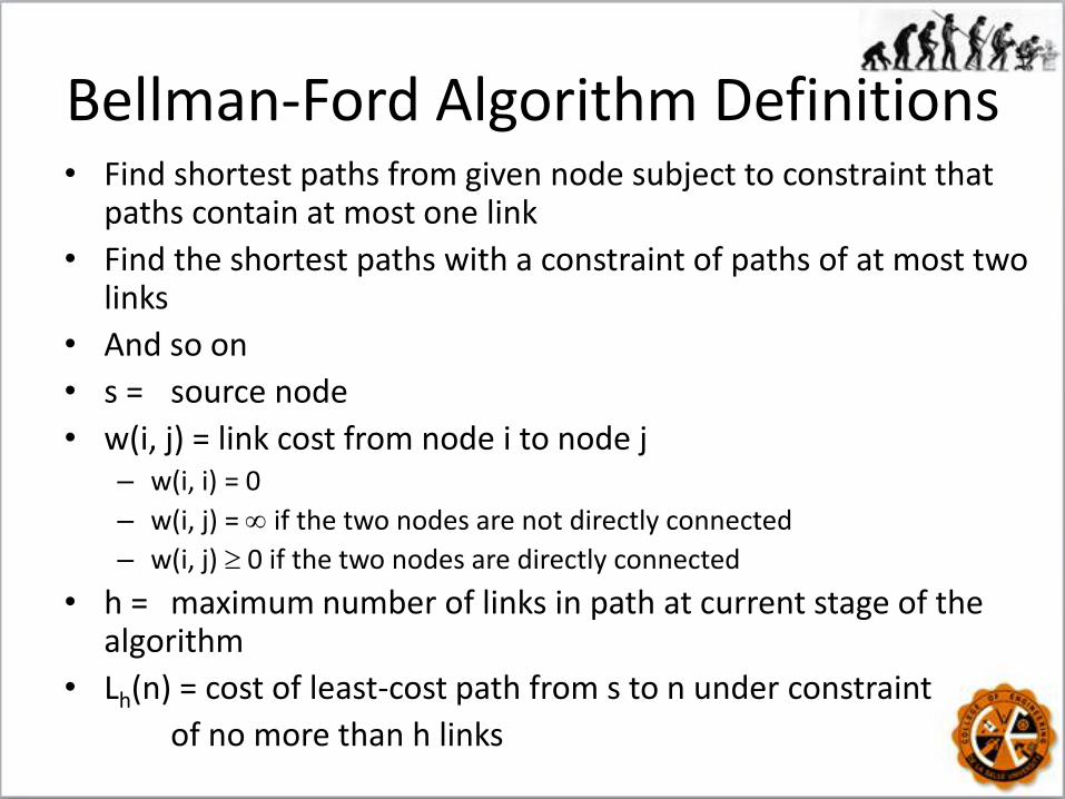
Bellman-Ford Algorithm Definitions • Find shortest paths from given node subject to constraint that
paths contain at most one link
• Find the shortest paths with a constraint of paths of at most two links
• And so on
• s = source node
• w(i, j) = link cost from node i to node j – w(i, i) = 0
– w(i, j) = if the two nodes are not directly connected
– w(i, j) 0 if the two nodes are directly connected
• h = maximum number of links in path at current stage of the algorithm
• Lh(n) = cost of least-cost path from s to n under constraint
of no more than h links

Bellman-Ford Algorithm
• Step 1 [Initialization] – L0(n) = , for all n s
– Lh(s) = 0, for all h
• Step 2 [Update]
• For each successive h 0 – For each n ≠ s, compute
– Lh+1(n)=minj[Lh(j)+w(j,n)]
• Connect n with predecessor node j that achieves minimum
• Eliminate any connection of n with different predecessor node formed during an earlier iteration
• Path from s to n terminates with link from j to n

Bellman-Ford Pseudocode
1 Bellman_Ford ( )
2 {
3 // Initialization
4 for (i = 1 to N; for j = 1 to N)
5 {
6 if(i == j) Dij = 0 cij = 0
7 else Dij = ∞ ; cij = cost
between i and j
8 }
9 // Updating 10 repeat 11 { 12 for (i = 1 to N; for j = 1 to N) 13 { 14 Dij ← minimum [(ci1 + D1j) ... (ciN + DNj)] 15 } // end for 16 } until (there was no change in previous iteration) 17 } // end Bellman-Ford
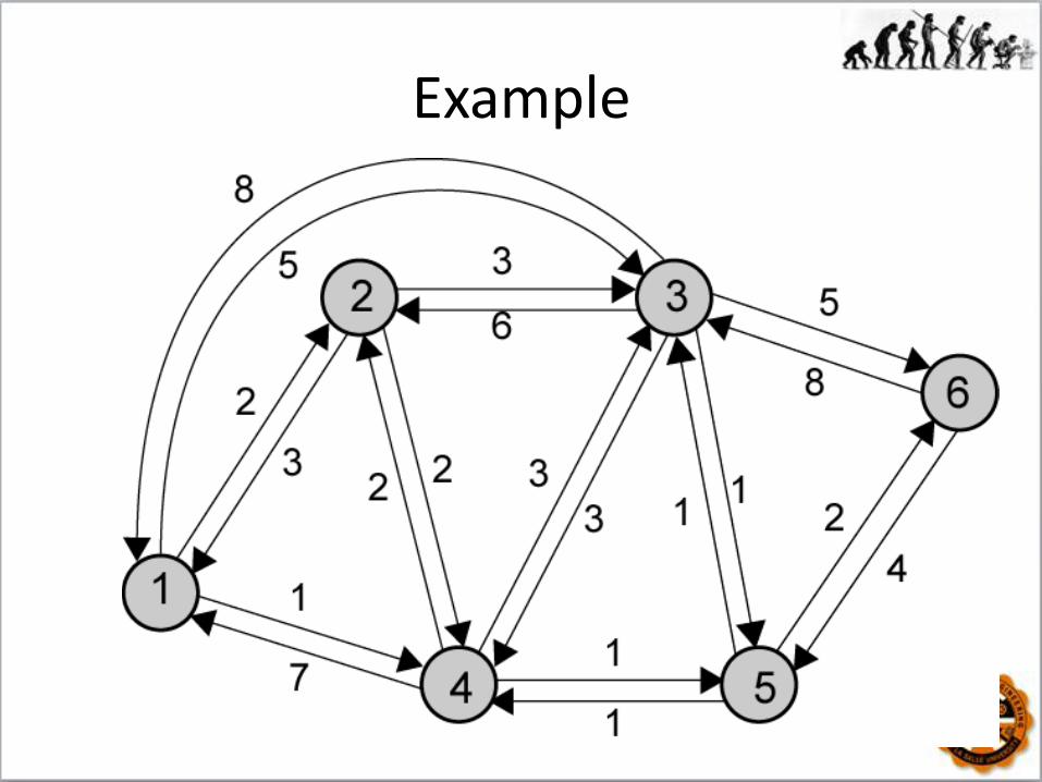
Example


Bellman-Ford Algorithm h Lh(2) Path Lh(3)
Path
Lh(4)
Path
Lh(5)
Path
Lh(6)
Path
0 - - - - -
1 2 1-2 5 1-3 1 1-4 - -
2 2 1-2 4 1-4-3 1 1-4 2 1-4-5 10 1-3-6
3 2 1-2 3 1-4-5-3 1 1-4 2 1-4-5 4 1-4-5-6
4 2 1-2 3 1-4-5-3 1 1-4 2 1-4-5 4 1-4-5-6
ARPANET Routing Strategies
• First Generation – 1969
– Distributed adaptive
– Estimated delay as performance criterion
– Bellman-Ford algorithm
– Node exchanges delay vector with neighbors
– Update routing table based on incoming info
– Doesn't consider line speed, just queue length
– Queue length not a good measurement of delay
– Responds slowly to congestion

ARPANET Routing Strategies
• Second Generation
– 1979
– Uses delay as performance criterion
– Delay measured directly
– Uses Dijkstra’s algorithm
– Good under light and medium loads
– Under heavy loads, little correlation between reported delays and those experienced

Dijkstra’s Algorithm Definitions • Find shortest paths from given source node to all other nodes,
by developing paths in order of increasing path length
N = set of nodes in the network
s = source node
T = set of nodes so far incorporated by the algorithm
• w(i, j) = link cost from node i to node j
– w(i, i) = 0
– w(i, j) = if the two nodes are not directly connected
– w(i, j) 0 if the two nodes are directly connected
• L(n) = cost of least-cost path from node s to node n currently known
– At termination, L(n) is cost of least-cost path from s to n

Dijkstra’s Algorithm Method • Step 1 [Initialization]
– T = {s} Set of nodes so far incorporated consists of only source node
– L(n) = w(s, n) for n ≠ s
– Initial path costs to neighboring nodes are simply link costs
• Step 2 [Get Next Node]
– Find neighboring node not in T with least-cost path from s
– Incorporate node into T
– Also incorporate the edge that is incident on that node and a node in T that contributes to the path

Dijkstra’s Algorithm Method
• Step 3 [Update Least-Cost Paths]
– L(n) = min[L(n), L(x) + w(x, n)] for all n T
– If latter term is minimum, path from s to n is path from s to x concatenated with edge from x to n
• Algorithm terminates when all nodes have been added to T
• At termination, value L(x) associated with each node x is cost (length) of least-cost path from s to x.

Example

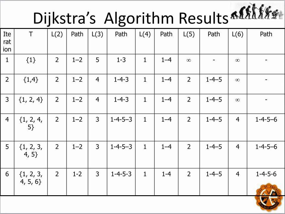
Dijkstra’s Algorithm Results Iteration
T L(2) Path L(3) Path L(4) Path L(5) Path L(6) Path
1 {1} 2 1–2
5 1-3 1 1–4 -
-
2 {1,4} 2 1–2
4 1-4-3 1 1–4 2 1-4–5
-
3 {1, 2, 4}
2 1–2
4 1-4-3 1 1–4 2 1-4–5
-
4 {1, 2, 4, 5}
2 1–2
3 1-4-5–3 1 1–4 2 1-4–5 4 1-4-5–6
5 {1, 2, 3, 4, 5}
2 1–2
3 1-4-5–3 1 1–4 2 1-4–5 4 1-4-5–6
6 {1, 2, 3, 4, 5, 6}
2 1-2
3 1-4-5-3 1 1-4 2 1-4–5 4 1-4-5-6
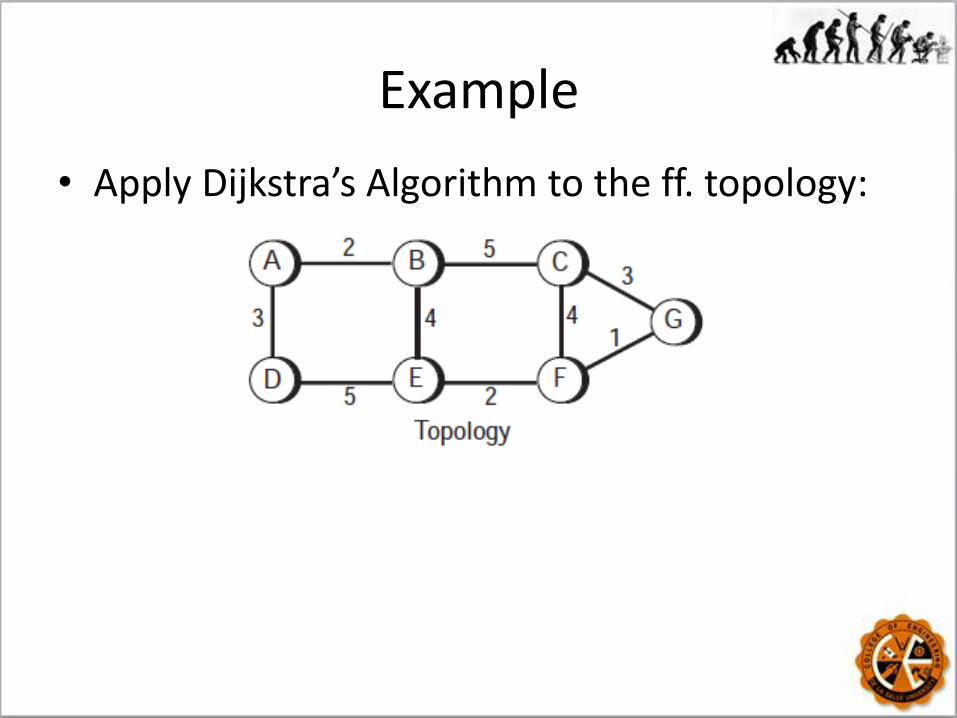
Example
• Apply Dijkstra’s Algorithm to the ff. topology:

Solution

Solution

Dijkstra’s vs. Bellman-Ford
– Bellman-Ford
• Calculation for node n involves knowledge of link cost to all neighboring nodes plus total cost to each neighbor from s
• Each node can maintain set of costs and paths for every other node
• Can exchange information with direct neighbors
• Can update costs and paths based on information from neighbors and knowledge of link costs
– Dijkstra
• Each node needs complete topology
• Must know link costs of all links in network
• Must exchange information with all other nodes
Distance Vector Routing Algorithm
• In distance vector routing, the cost is normally hop counts. So the cost between any two neighbors is set to 1.
• Each router needs to update its routing table asynchronously, whenever it has received some information from its neighbors.
• After a router has updated its routing table, it should send the result to its neighbors so that they can also update their routing table.

Distance Vector Routing Algorithm
• Each router should keep at least three pieces of information for each route: destination network, the cost, and the next hop.
• We refer to information about each route received from a neighbor as R (record), which has only two pieces of information: R.dest and R.cost.
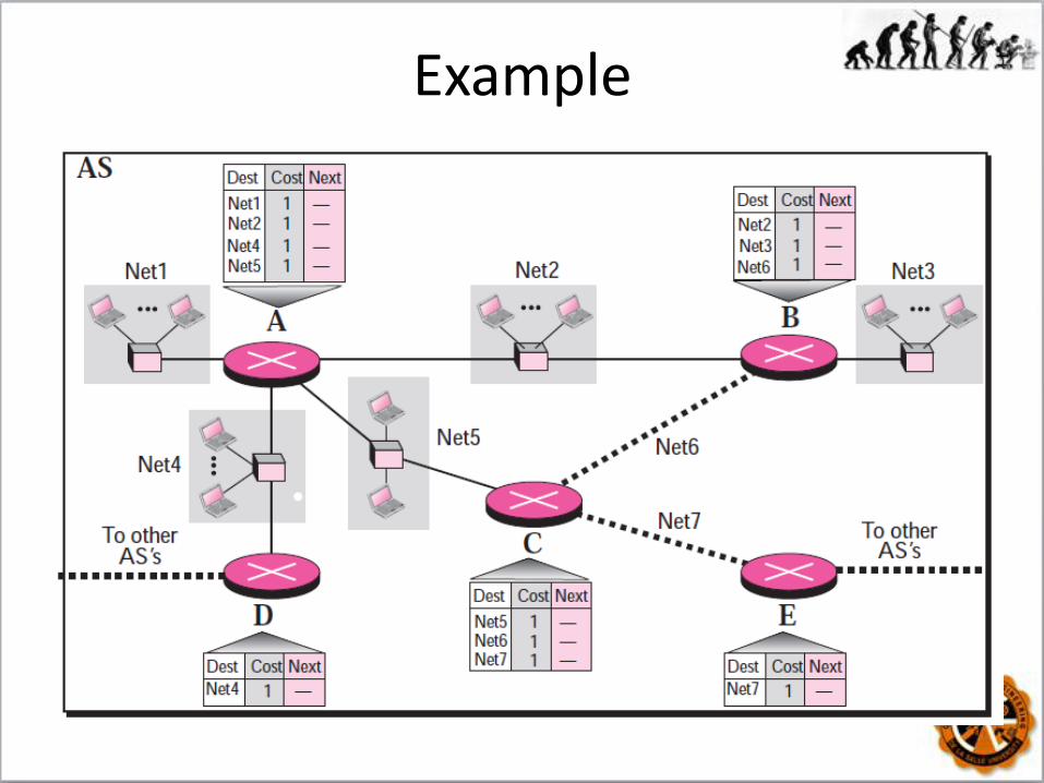
Example
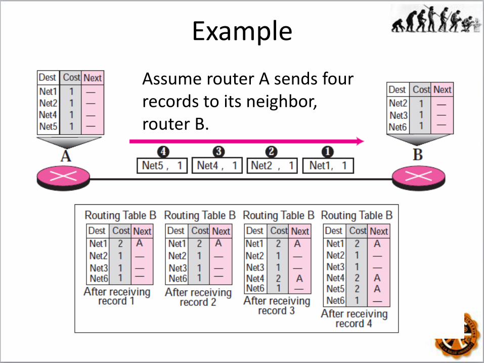
Example
Assume router A sends four records to its neighbor, router B.

Routing Information Protocol (RIP) • RIP is defined in RFC 1058, 1388, 1723 (RIP2)
• An intradomain (interior) routing protocol used inside an autonomous system.
• It is a very simple protocol based on distance vector routing.
• RIP implements distance vector routing directly.
• The distance is defined as the number of links (networks) that have to be used to reach the destination. The metric in RIP is called a hop count.

Routing Information Protocol (RIP)
• Infinity is defined as 16, which means that any route in an autonomous system using RIP cannot have more than 15 hops.
• The destination in a routing table is a network, which means the first column defines a network address.
• The next node column defines the address of the router to which the packet is to be sent to reach its destination.

Example

RIP Algorithm
If (destination not in the routing table)
Add the advertised information to the table.
Else
If (next -hop field is the same)
Replace entry in the table with the advertised one.
Else
If (advertised hop count smaller than one in the
table)
Replace entry in the routing table.
Return
Update Algorithm: Add one hop to the hop count for each advertised destination

RIP Message Format • Command. This 8-bit field specifies the type of
message: request (1) or response (2).
• Version. This 8-bit field defines the version.
• Family. This 16-bit field defines the family of the protocol used. For TCP/IP the value is 2.
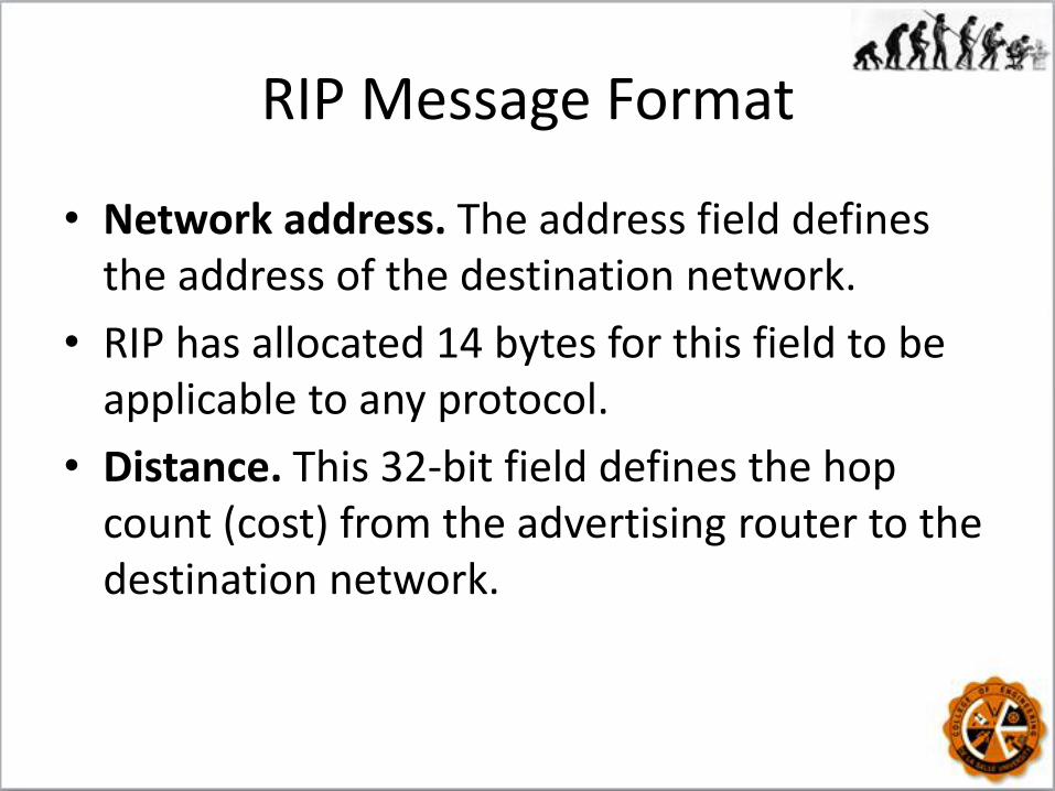
RIP Message Format
• Network address. The address field defines the address of the destination network.
• RIP has allocated 14 bytes for this field to be applicable to any protocol.
• Distance. This 32-bit field defines the hop count (cost) from the advertising router to the destination network.
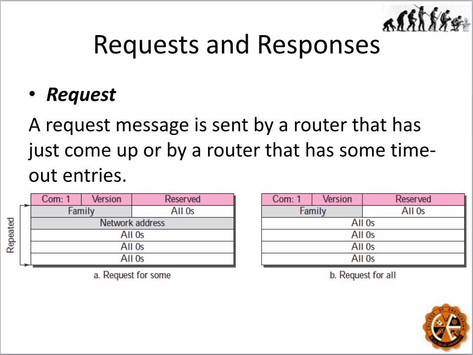
Requests and Responses
• Request
A request message is sent by a router that has just come up or by a router that has some time-out entries.

Requests and Responses
• Response A response can be either solicited or unsolicited. • A solicited response is sent only in answer to a
request. It contains information about the destination specified in the corresponding request.
• An unsolicited response, on the other hand, is sent periodically, every 30 seconds or when there is a change in the routing table.
• The response is sometimes called an update packet.

Example

RIP Version 2
• RIP version 2 was designed to overcome some of the shortcomings of version 1.
• The designers of version 2 have not augmented the length of the message for each entry.
• They have only replaced those fields in version 1 that were filled with 0s for the TCP/IP protocol with some new fields.
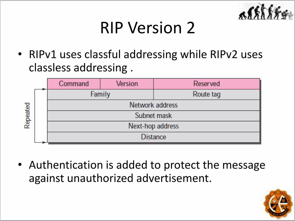
RIP Version 2
• RIPv1 uses classful addressing while RIPv2 uses classless addressing .
• Authentication is added to protect the message against unauthorized advertisement.

RIP Version 2
• Version 1 of RIP uses broadcasting to send RIP messages to every neighbor. All the routers on the network receive the packets, as well as the hosts.
• RIP version 2 uses the all-router multicast address to send the RIP messages only to RIP routers in the network.
Encapsulation
• RIP messages are encapsulated in UDP user datagrams.
• A RIP message does not include a field that indicates the length of the message. This can be determined from the UDP packet.
• RIP uses the services of UDP on well-known port 520.

Link State Routing
• If each node in the domain has the entire topology of the domain— the list of nodes and links, how they are connected including the type, cost (metric), and the condition of the links (up or down)—the node can use the Dijkstra algorithm to build a routing table.

Link State Routing
Link State Routing
• The topology must be dynamic, representing the latest situation of each node and each link.
• Link state routing is based on the assumption that, although the global knowledge about the topology is not clear, each node has partial knowledge: it knows the state (type, condition, and cost) of its links.
Building Routing Tables
• In link state routing, four sets of actions are required:
1. Creation of the states of the links by each node, called the link state packet or LSP.
2. Dissemination of LSPs to every other router, called flooding.
3. Formation of a shortest path tree for each node.
4. Calculation of a routing table based on the shortest path tree.
Link State Packet (LSP)
• LSP carries the node identity, the list of links, a sequence number, and age.
• Node identity and the list of links - are needed to make the topology.
• Sequence number - facilitates flooding and distinguishes new LSPs from old ones.
• Age - prevents old LSPs from remaining in the domain for a long time.

Understand
• LSPs are generated on which occasions?
Answer:
1. When there is a change in the topology of the domain.
2. On a periodic basis. (done to ensure that old information is removed from the domain)
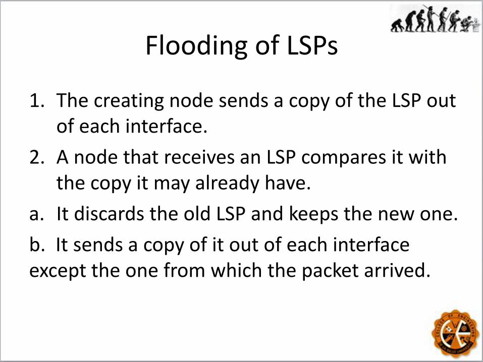
Flooding of LSPs
1. The creating node sends a copy of the LSP out of each interface.
2. A node that receives an LSP compares it with the copy it may already have.
a. It discards the old LSP and keeps the new one.
b. It sends a copy of it out of each interface except the one from which the packet arrived.
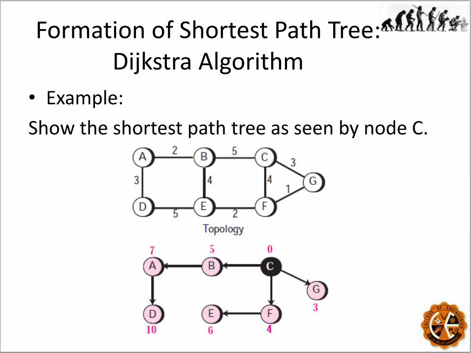
Formation of Shortest Path Tree: Dijkstra Algorithm
• Example:
Show the shortest path tree as seen by node C.
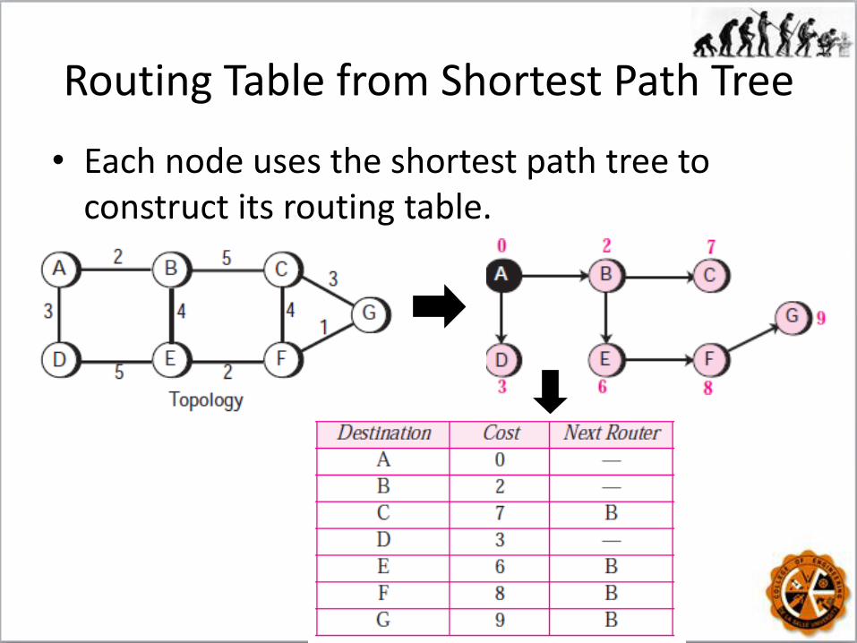
Routing Table from Shortest Path Tree
• Each node uses the shortest path tree to construct its routing table.

Open Shortest Path First (OSPF)
• An intradomain routing protocol based on link state routing.
• OSPF divides an autonomous system into areas.
• An area is a collection of networks, hosts, and routers all contained within an autonomous system.
• All networks inside an area must be connected.

OSPF
• Routers inside an area flood the area with routing information.
• At the border of an area, special routers called area border routers summarize the information about the area and send it to other areas.
• Backbone – a special area inside an AS where all of the other areas must be connected.

OSPF • The routers inside the backbone are called the
backbone routers.
• Each area has an area identification. The area identification of the backbone is zero.

OSPF Metric
• OSPF protocol allows the administrator to assign a cost, called the metric, to each route.
• The metric can be based on a type of service (minimum delay, maximum throughput, and so on).
• A router can have multiple routing tables, each based on a different type of service.

OSPF Links
• In OSPF, a connection is called a link.
• Point-to-point link - connects two routers without any other host or router in between.
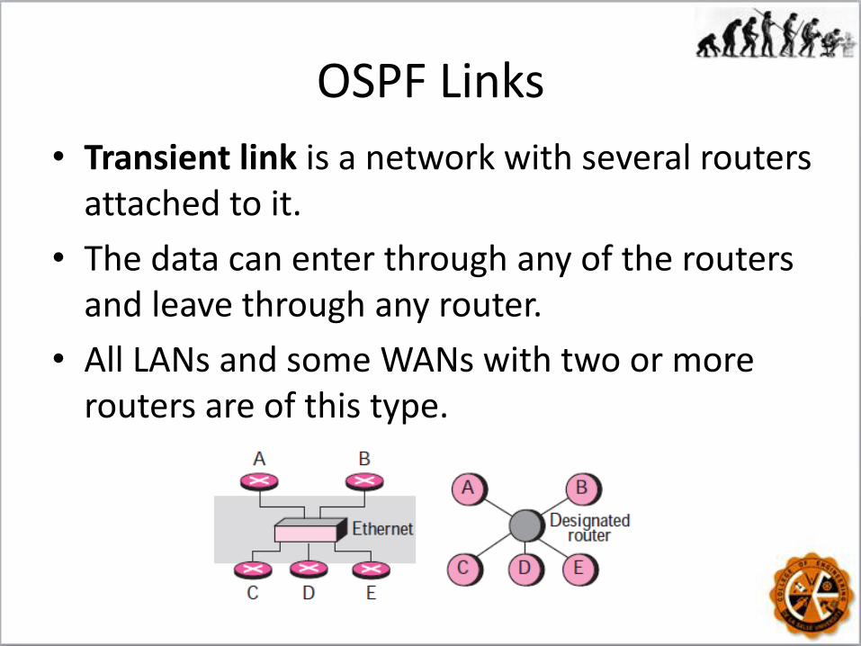
OSPF Links
• Transient link is a network with several routers attached to it.
• The data can enter through any of the routers and leave through any router.
• All LANs and some WANs with two or more routers are of this type.

OSPF Links • A stub link is a network that is connected to
only one router.
• The data packets enter the network through this single router and leave the network through this same router.
• A virtual link is created by the administration when the link between two routers is broken.
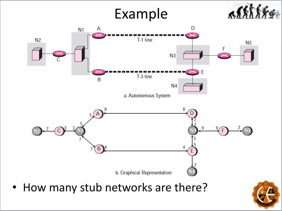
Example
• How many stub networks are there?
OSPF Packet Encapsulation
• OSPF packets are encapsulated in IP datagrams.
• They contain the acknowledgment mechanism for flow and error control.
• They do not need a transport layer protocol to provide these services.

Path Vector Routing • An exterior routing protocol for interdomain or
inter-AS routing.
• Recall: Distance vector and link state routing are both interior routing protocols.
• In distance vector routing, a router has a list of networks that can be reached in the same AS with the corresponding cost (number of hops).
• In path vector routing, a router has a list of networks that can be reached with the path (list of ASs to pass) to reach each one (path).
Analogy • The difference between the distance vector
routing and path vector routing can be compared to the difference between a national map and an international map.
• A national map can tell us the road to each city and the distance to be travelled if we choose a particular route;
• An international map can tell us which cities exist in each country and which countries should be passed before reaching that city.
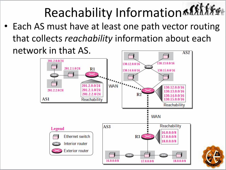
Reachability Information • Each AS must have at least one path vector routing
that collects reachability information about each network in that AS.

Routing Tables
• A path vector routing table for each router can be created if ASs share their reachability list with each other. Ex.
Path Vector Routing Features
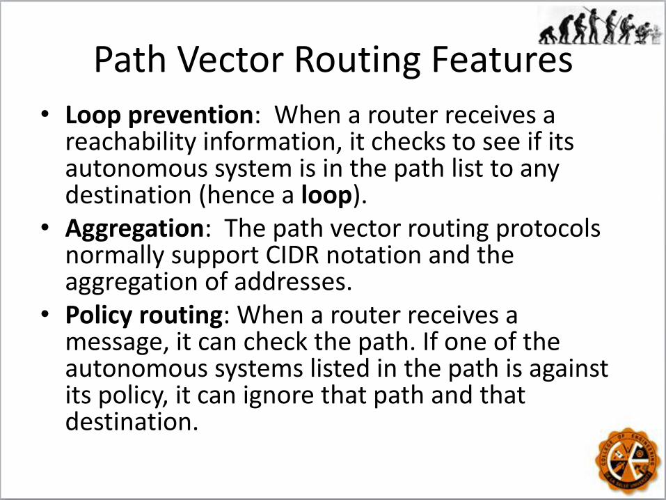
• Loop prevention: When a router receives a reachability information, it checks to see if its autonomous system is in the path list to any destination (hence a loop).
• Aggregation: The path vector routing protocols normally support CIDR notation and the aggregation of addresses.
• Policy routing: When a router receives a message, it can check the path. If one of the autonomous systems listed in the path is against its policy, it can ignore that path and that destination.

Border Gateway Protocol (BGP)
• An interdomain routing protocol using path vector routing.
• BGP uses classless interdomain routing addresses (prefix-based).
• The exchange of routing information between two routers using BGP takes place in a session.
• A session is a connection that is established between two BGP routers only for the sake of exchanging routing information.
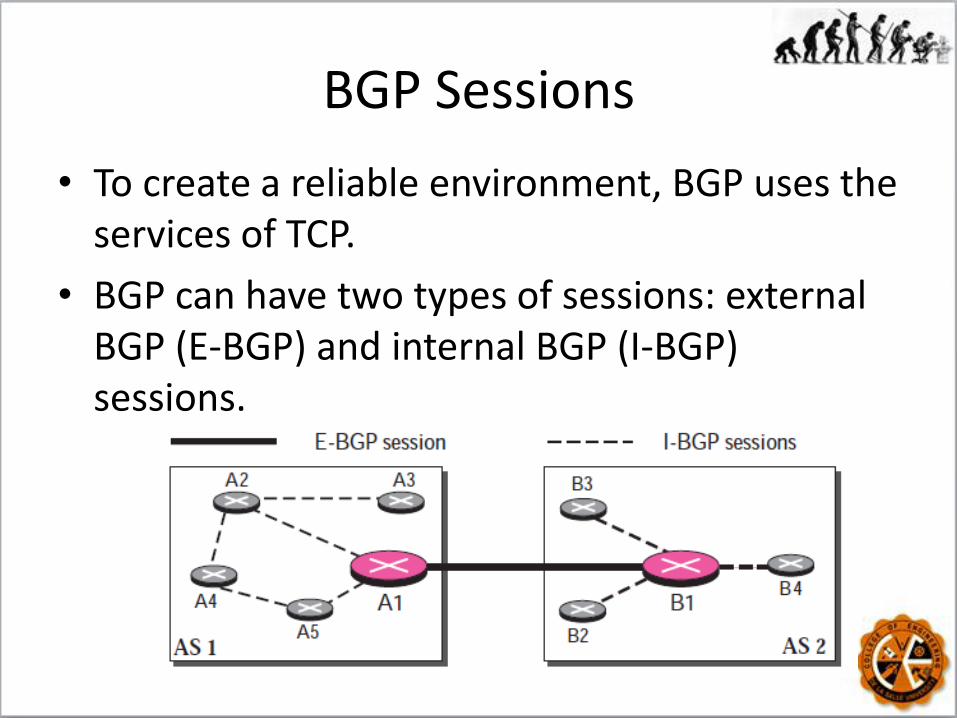
BGP Sessions
• To create a reliable environment, BGP uses the services of TCP.
• BGP can have two types of sessions: external BGP (E-BGP) and internal BGP (I-BGP) sessions.
Reading Assignment
• The types of OSPF packets and their formats.
• The types of BGP packets and their formats.
Hint: There are four types of BGP messages: open, update, keepalive, and notification.
• Multicasting and Multicast Routing Protocols
Multicast Link State Routing (MOSPF),
Multicast Distance Vector Routing, etc.

RFCs
• RIP is discussed in RFC1058, RFC1388, RFC1723 and RFC 2453.
• OSPF is discussed in RFC 1583 and RFC 2328.
• BGP is discussed in RFC 1654, RFC 1771, RFC 1773, RFC 1997, RFC 2439, RFC 2918, and RFC 3392.

End