
Roughness and Reflection in Machine Vision and Reflection in Machine Vision Ronald A. Stone July...
157
Roughness and Reflection in Machine Vision Ronald A. Stone CMU-€3-TR-94-41 The Robotics Institute Carnegie Mellon University Pittsburgh, Pennsylvania 15213 July 1994 0 1994 by Ronald A. Stone. All rights reserved This research was sponsored by the Avionics Laboratory, Wright Research and Development Center, Acronautical Systems Division (AFSC). U.S. Air Force, Wright-Patterson AFB, OH 45433-6543 under Contract F33615-9o-C-1465, Arpa Order No. 7597. The views and conclusions contained in this document are. thwe of the author and should not be interpreted as representing the official policies. either expressed or implied. of the United States Government.
Transcript of Roughness and Reflection in Machine Vision and Reflection in Machine Vision Ronald A. Stone July...

Roughness and Reflection in Machine Vision
Ronald A. Stone
CMU-€3-TR-94-41
The Robotics Institute Carnegie Mellon University
Pittsburgh, Pennsylvania 15213
July 1994
0 1994 by Ronald A. Stone. All rights reserved
This research was sponsored by the Avionics Laboratory, Wright Research and Development Center, Acronautical Systems Division (AFSC). U.S. Air Force, Wright-Patterson AFB, OH 45433-6543 under Contract F33615-9o-C-1465, Arpa Order No. 7597.
The views and conclusions contained in this document are. thwe of the author and should not be interpreted as representing the official policies. either expressed or implied. of the United States Government.

Roughness and Reflection in Machine Vision
Ronald A. Stone
July 1994
Department of Physics Camegie Mellon University
Pittsburgh, Pennsylvania 15213
Submitied in partiuEfu@llrnent of the requirements for the degree of Doctor of Philosophy
Thesis committee: Chair: Steven Shafer, Associate Professor, Carnegie Mellon University
Ned VanderVen, Professor, Carnegie Mellon University Stephen Garoff, Professor, Carnegie Mellon University
Michael Fuhnnan, The Aluminum Company of America
Copyright 0 1994 by Ronald A. Stone
This research was sponsored by the Avionics Laboratory, Wright Research and Development Center, Aeronautical Systems Division (AFSC), U.S. Air Force, Wright-Patterson AFB, OH 45433-6543 under Contract F33615-90-C- 1465, Arpa Order No. 1591.
The views and conclusions contained in this document are those of the author and should not be interpreted as repre- senting the official policies, either expressed or implied. of the U.S. Government.


Abstract
We want to develop algorithms which allow a computer vision system to qualitatively esti-
mate the roughness of reflective surfaces from a single image, under normal lighting conditions,
and with incoherent light. In order to make such a system applicable to most imaging situations,
we attempt to constrain the environment as little as possible, and thus, we will study the reflected
images of step edges, since these are ubiquitous and algorithms for their detection are mature.
We first derive a six-parameter model of reflected step edges, and show that with this model it
is possible to differentiate surfaces by roughness. In order for this differentiation to be correct,
however, certain information about the imaging geometry must be known; we list what informa-
tion is necessary, and describe the effect of changes in these parameters on the appearance of
reflected edges.
We then use this knowledge of the appearance of the reflected edges to develop two methods
of roughness estimation. The first method fits a curve described by the six-parameter model to the
reflected edge profile data by a combination of gradient descent and singular value decomposition
algorithms. The output of this algorithm is the best-fit values of the six parameters, one of which
is the root-mean-square slope of the surface, which we use to quantify the roughness. We then dis-
cuss the imaging conditions for which this algorithm works well. The next method of roughness
estimation treats the equation for the reflected radiance as a first kind Volterra integral equation.
After solving the integral equation, it calculates a quantity which allows it to order surfaces by
roughness. Although it does not calculate the roughness directly, as the first method does, it works
for many imaging situations for which the first algorithm does not.

page iu
We test these algorithms on the images of step edges reflected in the surfaces of five steel
disks of different roughness. We measure the root-mean-square slopes of these surfaces with a
proflometer and compare the output of our algorithms with these values. We find that both algo-
rithms order the surfaces correctly by roughness.

Acknowledgments
There are many people without whose help this thesis would not be. I would like to thank the
members of my committee, starting with my advisor, Steve Shafer. Steve has never ceased to
amaze me with his ability to generate interesting new directions for research, and his knack of
quickly grasping the essentials of any problem. This thesis would have been much less in every
sense without his help. I owe a great debt of gratitude ro Steve Garoff, who put in a level of effort
more appropriate to an advisor than a committee member. I would l i e to thank Michael Fuhrman
for all his help with my research. His comments were always remarkably insightful; his experi-
ence with technical issues was greatly appreciated. I would also like to express my thanks to Ned
VanderVen for his knowledgable comments and suggestions throughout my years at Camegie
Mellon.
I owe much to the people who helped with the technical aspects of my research. I would like
to thank Michael’s employer, the Aluminum Company of America, for its generous loan of the
steel disks which we used as the samples for our experiments. I am also indebted to Chris Bow-
man for giving me free rein of the clean room and the profilometer.
Many others have contributed over the years, in ways both large and small. I would like to
thank Roland Heid, O.S.B., for initially s p a r b g my interest in optics. He is a great teacher. The
other members of the Calibrated Imaging Lab, John Krurnm, Carol Novak, Reg Willson, Bruce
Maxwell, and Yalin Xiong, provided friendship as well as fascinating discussions about computer
vision. I would like to thank all my office mates over the years, as well as the whole gang in the
Physics department: Guru, Brent, Conrad, Dan, Raouli, Doros, and all the rest. I am especially

page v
grateful to the people who kept things running: Jim Moody, Bill Ross, Ralph Hyre, and Patty
Mackiewicz.
Finally, I would like to thank the really important people. First, my family, who have never
ceased providing support for the past twenty-eight years. I know I would not have been able to do
nearly as much as I have without the support of my parents, my brothers, my sister, and my great
aunt. Most of all, I would like to thank my fiance, Janet Bricmont, for her constant patience during
the writing of this thesis.

Ad Mujorern Dei Glonam

Contents 1 . Introduction 1
1.1 Background ................................................................................................................... 2
1.1.2 Applications to Computer Vision .......................................................................... 3 ...................................................... 1 . 1. 1 The Scattering of Light from Rough Surfaces 2
1.1.3 Our Research ........................................................................................................ 6 1.2 Thesis Outline ................................................................................................................ 7
9 2.1 Chapter Overview ......................................................................................................... 9 2.2 What is roughness? ....................................................................................................... 9
2.2.1 Roughness Statistics ............................................................................................ 9
2.3 The Reflection ofLight ................................................................................................ 14
2 . Roughness and Reflection
2.2.2 Roughness Models ............................................................................................ 12
2.3.1. The Theory of Reflection in the Physical Optics Regime .................................. 14 2.3.2. The theory of reflection in the geometrical optics reghe ................................ 17
2.4. Our Choice of Model .................................................................................................. 22 2.5. Conclusions ................................................................................................................ 24
3 . Edges 25 3.1. Chapter Overview ....................................................................................................... 25 3.2. Edges as an Extended Source ..................................................................................... 25 3.3. Limitations on the Differentiation of Edges ............................................................. 34
3.3.2. The Effect of Changes in the Source-Object Distance ...................................... 38 3.3.3. The Effect of Changes in the Viewing Angle ................................................... 41 3.3.4. The Effect of Changes in the Specular Spike Width ......................................... 43 3.3.5. Ambiguous Edges .............................................................................................. 44
3.4. The Effect of Surface Shape ........................................................................................ 47 3.5. Conclusions ................................................................................................................ 49
51 4.1. Chapter Overview ...................................................................................................... 5 1 4.2. The Algorithm ............................................................................................................ 51 4.3. The Surfaces ............................................................................................................... 57
4.3.1. Height and Slope Statistics ................................................................................ 57
4.4. Experimental Setup .................................................................................................... 68
4.6. Summary and Discussion ........................................................................................ ..88
89 5.1. Chapter Overview ....................................................................................................... 89 5.2. Shortcomings of the Iterative Method ........................................................................ 89 5.3. Reflected Radiance Equation ..................................................................................... 96
5.3.1. Modified Reflected Radiance Equation ............................................................ 96
3.3.1. Source-Object-Camera Configuration for the Simulations ............................... 35
4 . An Iterative Roughness Estimation Method
. . . 4.3.2. Height Distributions .......................................................................................... 63
4.5. Analysis of the Fitted Parameters .............................................................................. 77
5 . A Direct Roughness Estimation Method

5.3.2. Solution of the Modified Reflected Radiance Equation .................................. 101 5.4. Width Measures ........................................................................................................ 104
5.4.1. The Variance ................................................................................................... 104 5.4.2. Our Width Measure ......................................................................................... 108 5.4.3. The Effects of Noise ........................................................................................ 110
5.5. Experiment ............................................................................................................... 111 5.5.1. Experimental Configuration ............................................................................ 111
5.5.3.OldData ........................................................................................................... 116 5.5.4. New Images ..................................................................................................... 116
5.6. Conclusions .............................................................................................................. 126
128 6.1. Summary .................................................................................................................. 128 6.2. Contributlons ............................................................................................................ 128 6.3. Directions for future. research .................................................................................... 131 6.4. Concluding Remarks ................................................................................................ 132
7 . Bibliography 133
8 . Appendix 1 136
9 . Appendix 2 139
5.5.2. The Direct Roughness Estimation Algorithm .................................................. 113
6 . Summary and Conclusions
. .

List of Figures
1: Venn diagram of roughness models ..................................................................................... 13 2: The geometry for the scattering of light waves ..................................................................... 15 3: A rough surface comprised of mirror-like facets .................................................................. 18
under the assumption of geometrical optics models .............................................................. 18 5: The illumination environment for several points on a surface .............................................. 26
7: The one-dimensional reflection geometry ........................................................................... 28
Gaussian of approximately the same width ........................................................................... 32 9: Schematic of the simulation configuration ........................................................................... 35 10 Edges for several values of beta ......................................................................................... 37 1 1: Diagram to accompany the derivation of the angle for our simulations ............................. 39 12: Edges for several values ofbeta ......................................................................................... 40 13: Edges for several values of beta ........................................................................................ 40 14: Edges for several values of er .......................................................................................... 42
15: Edges for several values of er ........................................................................................... 42
4 The reflection geometry for the derivation of the scattered light intensity,
6: The reflection geometry ....................................................................................................... 27
8: The central lobe of the square of the sinc function and a
16: Edges for several values of 8, ............................................................................................ 43
17: Edges for several values of alpha ........................................................................................ 18: Two edge profiles with different parameter sets ................................................................ 45 19: Partoftheedgeprofilesforbetaequalto0.15 andO.20. .................................................... 46 20: Incidence and viewing angles for a curved surface ............................................................ 49 21: A schematic of the experimental configuration .................................................................. 52 22: The reflection geometry for the experimental configuration .............................................. 53 23: The initial guesses for the parameters A , B , and c for an edge profile ............................... 56 24: Relationship between the facet slope and the angle of the normal ...................................... 62 25: Number of occurrences of each height value, 1.5 microinches roughness sample .............. 64 26: Number of occurrences of each height value, 3.0 microinches roughness sample .............. 64 27: Number of occurrences of each height value, 4.5 microinches roughness sample .............. 65 28: Number of occurrences of each height value, 7.5 microinches roughness sample .............. 65 29: Number of occurrences of each height value, 9.5 microinches roughness sample .............. 66 30: Schematic of the experimental configuration ..................................................................... 69 31: The reflected image of the step edge in the 1.5 microinches sample
and the 3.0 rmcroinches sample .......................................................................................... 71 32: The reflected image of the step edge in the 4.5 microinches sample
33: The reflected image of the step edge in the 9.5 microinches sample .................................. 72 34: The average of the scanlines, 1.5 microinches roughness sample ...................................... 73 35: The average of the scanlines, 3.0 microinches roughness sample ...................................... 74 36: The average of the scanlines, 4.5 microinches roughness sample ...................................... 74 37: The average of the scanlines, 7.5 microinches roughness sample ...................................... 75 38: The average of the scanlines, 9.5 microinches roughness sample ...................................... 75
. .
. . and the 7.5 mcroinches sample .......................................................................................... 72

39: Best fit reflected edge profile anderror bars for 1.5 microinches roughness sample .......... 78 40: Best fit reflected edge profile anderror bars for 3.0 microinches roughness sample .......... 79 41: Best fit reflected edge profile anderror bars for 4.5 microinches roughness sample .......... 80 42: Best fit reflected edge profile anderror bars for 7.5 microinches roughness sample .......... 81 43: Best fit reflected edge profile anderror bars for 9.5 microinches roughness sample .......... 82
for the 1.5 microinches roughness sample ......................................................................... 85 45: Average reflected edge profile for the 1.5 microinches roughness sample ......................... 91 4 6 Best fit curve and error bars for 1.5 microinches roughness sample ................................... 91 47: Best fit edge profile and error bars for image number eight ................................................ 93 48: Best fit edge profile and error bars for image number eight ................................................ 93
and the error bars for image number eight .......................................................................... 94
into the camera for different points on the surface .............................................................. 98
44: A close-up view of part of the best fit curve and error bars
49: The average edge profile for image number five,
50: Different groups of facets will reflect light from the source
51: Schematic of the experimental configuration ................................................................... 112 5 2 The reflection geometry for the experimental configuration ............................................ 112 53: Geometry for the calculation of the viewing angle as a function of position .................... 114 5 4 The function u[el) for the 1.5 microinches roughness sample .......................................... 117
55: The function we,) for the 3.0 microinches roughness sample .......................................... 117
5 6 The function “e? for the 4.5 microinches roughness sample ......................................... 118
57: The function u(e+ for the 7.5 microinches roughness sample ........................................ 118
58: The function we+ for the 9.5 microinches roughness sample ......................................... 119
59: The function u(e,) for image 1 ......................................................................................... 120
6 0 The function u[e? for image 2 .......................................................................................... 121
61: The function u[e? for image 3 .......................................................................................... 121
62: The function u[e) for image4 .......................................................................................... 122
63: The function u[e+ for image 5 .......................................................................................... 122 I
64: The function u[e+ for image 6 .......................................................................................... 123
65: The function u(e3 for image 7 .......................................................................................... 123
66: The function u[e+ for image 8 .......................................................................................... 124
67: The function u(e2 for image 9 .......................................................................................... 124

List of Tables
1: Measured rms roughness value ............................................................................................ 59 2: Calculated correlation length ............................................................................................... 60 3: Estimate of the root-mean-square slope ............................................................................... 61 4 Mean height and roughness parameter ................................................................................. 67 5:Best fit values of the parameters ........................................................................................... 77 6: Chi squared value for the fit ................................................................................................. 83 7:: The calculated rms slope for the 1.5 microinches roughness sample
8:: The value of w for the five samples . 9:: The width measure w for the images of the 1.5 microinches roughness sample ............... 125
for several source-object-camera configurations ................................................................ 92
The images used are the same as those in Chapter 3 .......................................................... 119


1. Introduction
Many things can influence the appearance of an image recorded by a camera, such as the
lighting, the lens settings of the camera, and the properties of the objects in the scene. One impor-
tant property which is presently a subject of much research in the field of physics-based vision is
the effect of the roughness of reflective surfaces on their appearance. A complete description of
the change in the reflective properties of surfaces with respect to roughness is of theoretical inter-
est, but also has practical applications, from quality control in factories to general purpose vision
systems, in which a robot attempts to gain information about its environment. The estimation of
roughness could also aid a robotic vision system in material type classification and image seg-
mentation, and thus could be one of the low-level steps in a complete vision system. Obviously,
the understanding of the effects of surface roughness on object appearance and the development
of roughness estimation algorithms is important to the advancement of computer vision research.
This thesis will address many of the issues of the effects of roughness on the appearance of
reflective surfaces. It will study the reflected images of step edges, since these are present in many
environments and are one of the most thoroughly studied and commonly used image features. It
will present a model of the reflected images of step edges, and will show the effects of surface
roughness on the appearance of the edges. Finally, it will discuss the minimum amount of infor-
mation necessary for the estimation of surface roughness from edges, and will present algorithms
that estimate the roughness of a reflective surface by studying a single image of the surface con-
taining the reflection of one or more step edges.

page 2
1.1. Background
Although the analysis of the reflection of light from rough surfaces has a long history, the
application of this knowledge in the computer vision field for the analysis of the appearance of
rough surfaces occurred more recently. Theories of reflection found use in constrained laboratory
settings from their inception, but the computational complexity inherent in most computer vision
applications precluded their immediate use. As computational capabilities increased, however,
computer vision researchers were able to use more complete and physically meaningful descrip-
tions of reflection.
1.1.1. The Scattering of Light from Rough Surfaces
The study of the reflection of light from rough surfaces has its origin in the analysis of radar
reflected from rough ground and the ocean. Rice performed some of the first work in this area
shortly after the Second World War.[Rice 511 He assumed that the reflective surfaces had low
slopes, and with this simplification, he was able to solve for the scattered light intensity. Addition-
ally, he studied special cases of surface shape, such as sinusoids. His theory is presently important
in the measurement of the roughness of very smooth surfaces, such as lenses and other optical ele-
ments.[Stover 901
In 1963, Beckmann and Spizzichino proposed a model of the scattering of elecaomagnetic
waves from rough surfaces which used a different set of assumptions.[Beckmann and Spizzichino
631 Their theory dealt with surfaces which have a Gaussian distribution of height values, and the
calculations relied heavily on statistical methods. They derived a series solution for the scattered
intensity pattern. This theory works well for surfaces that are rougher than those dealt with by
Rice’s theory. With the advent of optical profilometers, this theory has gained favor with those

page 3
measuring the roughness of metal surfaces, and is now probably the most used description of
rough surface scattering among those researchers.
Both Rice’s and Beckmann and Spizzichino’s theories treat light as a wave phenomenon. It is
possible in some cases, however, to describe the reflection of the light by the laws of geomemcal
optics. Beckmann introduced such a description [Beckmann 571, and Du Castel and Spizzichino
improved upon it.[Du Castel and Spizzichino 591 In 1967, Torrance and Sparrow porrance and
Sparrow 671 used a geomeaical description of reflection to explain the existence of “off-specular
peaks” in the scattering patterns they found for rough metal surfaces, and showed how these
peaks could result from the shadowing of surface “microfacets” by one another. The calculations
involved in these geomemcal optics theories are often simpler than those of wave theories such as
Rice’s and Beckmann and Spizzichino’s. This accounts for much of their ppularity. As shown by
Beckmann and Spizzichino, however, limiting cases of their wave theory have an equivalent geo-
metrical optics formulation, thus making their wave optics theory as easy to use as the geometri-
cal optics theoIy in these cases.
Research into theories of the reflection of light from rough surfaces continues to this day. New
surface models, such as fractal descriptions of surfaces [Jaggard and Sun 901 , are popular. Most
of the new theories have not yet influenced the field of computer vision.
1.1.2. Applications to Computer Vision
At different stages in the history of computer vision and computer graphics research, particu-
lar ones of these theories of reflection from rough surfaces have enjoyed popularity.
Starting in the 1970’s, computer graphics researchers began studying reflection from rough
surfaces in order to create increasingly realistic images. They searched for theories which would

page 4
not only make convincing pictures, but which were also simple enough to use with the limited
computational power of the times. One of the first of these models was proposed by
Phong.[Phong 751 In this description, the distribution of the reflected light intensity, L , is given
by L = (case) ', where e represents the angle between the normal to the surface and the bisector
of the directions of the incident and reflected light rays, and n is a number greater than 1. Increas-
ing values of n represent decreasing roughness. There is little physical basis for this model, but
the resulting images were quite good for the time.
As computational power increased, many in the computer graphics field saw the need for bet-
ter descriptions of rough-surface reflection. The Torrance and Sparrow theory of reflection
became popular at this time. Blinn was the fist to use this theory to generate realistic images of
rough metallic objects.[Blinn 771
Researchers in the computer vision field also saw the potential of the Torrance and S p m w
geometrical optics theory for solving the inverse problem, that is, finding the roughness of a sur-
face from its reflected radiance distribution. One of the first applications of this theory in com-
puter vision was the work of Healey and Binford [Healey and Binford 871, in which rough
cylindrical metal surfaces were imaged under point source illumination. The intensity pattern
across the cylinder yielded the roughness as well as the radius of curvature of the surface.
The Torrance and S p m w theory has found use more recently in the photometric sampling
research of Ikeuchi and his collaborators.[Kiuchi and Ikeuchi 93][Solomon and Ikeuchi911
[Nayar et al. 881 Photomemc sampling is an experimental technique in which an object is illumi-
nated from several directions in turn, but viewed from a single direction. The illumination is usu-

page 5
ally a point source, although the method can work with extended sources. Analysis of the
resulting images allows the determination of the object shape and roughness.
The need for multiple images, small samples, and specialized equipment make the photomet-
ric stereo technique unsuitable for general purpose vision systems. Ikeuchi and Sat0 have intro-
duced a method of roughness estimation which uses the Torrance and Sparrow theory, and which
requires only a single image under point source illumination of the object being studied.[nEeuchi
and Sat0 911 It does, however, require knowledge of the object shape, and this is obtained with a
laser rangefinder.
Novak also used the Torrance and Sparrow theory in her analysis of the color histograms of
reflective dielectric surfaces.[Nov& 921 The analysis yielded the roughness of the surfaces, but it
required that the body reflection of the surfaces be Lambertian, SO that the shape of the object
could be estimated
Further increases in the power of computers allowed researchers to move from the Torrance
and Sparrow geometrical optics theory of reflection to the Beckmann and Spizzichino wave optics
theory. Cook and Torrance w e n the first to use this theory for computer graphics.[Cook and Tor-
rance 821 However, they used a simplified version of this theory which was also derived by Beck-
mann and Spizzichino.
Mundy and Porter were the first to use the theory of Beckmann and Spizzichino in a computer
vision setting.wundy and Porter 801 They developed a method for the detection of defects on
metal surfaces. Their method was similar to that of photometric stereo in that it calculated the
roughness of surfaces from multiple measurements of the reflected intensity made with different

page 6
point light source directions. Like Cook and Torrance, they also used a simplified version of the
theory.
Nayar used simulations to thoroughly study the wave optics theory of reflection. Thus he was
the first to use the complete theory of Bechann and Spizzichino in a computer vision setting.
[Nayar et a!. 911
1.1.3. Our Research
There are shoncomings to all of the methods of roughness estimation listed above. First, many
of the methods require multiple images of the reflective surface under study. The ability of
humans to estimate the roughness of surfaces does not have this constraint; most people can guess
the roughness of a surface from a single image. We believe that this ability is largely a matter of
pattern recognition, and that with the analysis of the proper image features, we may design algo-
rithms which determine roughness from a single image. Another shortcoming is that in all of the
methods of roughness estimation described above, the researchers have used point light sources.
Although point light sources are present in some imaging environments, they are not as common
as many researchers would like to believe. In order to overcome these problems, our roughness
estimation methods will analyze single images containing the reflections of step edges.
There are several reasons for our choice of studying step edges. We believe that edges are
more common than point light sources. Additionally, step edges will be present in many environ-
ments, particularly those containing artificial objects. Finally, the methods of edge detection and
analysis are mature, and are a common first step in many computer vision systems. Therefore, our
methods will not require additional preprocessing steps.

page 7
In our research, we will use the Beckmann and Spizzichino model of reflection, since it is one
of the most complete theories of reflection from rough surfaces, and because it has a geometrical
optics fornulation which is easy to use.
1.2. Thesis Outline
In the second chapter of the thesis, we discuss rough surfaces and the reflection of light from
such surfaces. We begin by describing some of the different ways of pmameterizing rough sur-
faces, and the statistics commonly used to quantify roughness. The chapter continues with a
description of the different theories of the reflection of light from rough surfaces and how certain
theories of reflection necessitate the use of certain surface parameterizations. We discuss in detail
the model we will use in most of our work to describe rough surfaces and the theory we use to
study the reflection of light from them.
In Chapter 3., we take up the subject of the reflected images of edges, the image feature
around which we will build our work. We derive an equation which describes the appearance of
the reflected edge image in a rough surface, and identify certain parameters, such as the shape of
the reflective surface and the viewing angle, which greatly influence the reflected edge profile.
Following this is a discussion of how variations in these parameters change the appearance of the
reflected edge image. Simulations of reflected edge profiles accompany this discussion. We also
show that there exist different parameter sets which produce reflected edges that appear almost
indistinguishable, and conclude that the values of these parameters must be known for any
method of roughness estimation to give accurate answers.
Chapter 4. introduces a six-parameter model of the profile of a reflected edge image. We then
present our first method of roughness estimation; the algorithm fits a cunre for OUT model to a

Page 8
reflected edge profile. It iteratively finds the best fit solution, and from this we may read off the
surface roughness. We test our method on several surfaces with different, known roughnesses.
The results of the algorithm are then compared with roughness values found by stylus profilome-
try, a common roughness measurement method
We begin Chapter 5. by giving examples of the reflected images of edges for which the itera-
tive solution method of roughness estimation does not work. After explaining why the method
failed in these cases, we introduce a second method of roughness estimation which is basal on the
theory of first-kind Volterra equations, and which can order surfaces by roughness. We show that
this new method works on the images for which the first method did not.
In the Summary and Conclusions chapter, we reiterate the important findings of this thesis and
discuss areas for future research.

2. Roughness and Reflection
2.1. Chapter Overview
Our study of the reflection of light from rough surfaces begins with a discussion of the defini-
tion of roughness. This is not as simple as it may seem at fist, and our choice of definition for
roughness often influences our choice of method for solving for the radiance of the reflected light.
We then discuss the physical-optics and geometrical-optics approaches to quantifying the reflec-
tion of light from surfaces. We choose to model rough surfaces as having a Gaussian distribution
of height values. We feel that this model adequately describes many real surfaces, and reflection
from such surfaces may be treated by both the methods of physical optics and geometrical optics.
2.2. What is roughness?
In order to study the reflection of light from rough surfaces, we must first define what we
mean by roughness. This is no easy task; myriad definitions exist, and each has its usefulness. Let
us describe a few of the most common definitions of roughness.
2.2.1. Roughness Statistics
Perhaps the most common way to quantify the roughness of a surface is to calculate the values
of some common statistical parameters for the surface. Let us assume, for ease of pedagogy, that
the rough surface under study is a one-dimensional function, Le. we know its height, h(x), for
every position, x . Ow definitions will hold for two-dimensional surfaces with minor modifica-
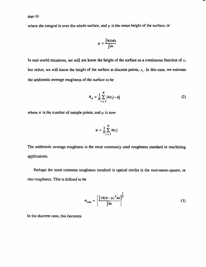
tions. The arirhmeric average roughness of the surface is defined to be [Stover 901
page 10
where the integral is over the whole surface, and p is the mean height of the surface, or
In real-world situations, we will not know the height of the surface as a continuous function of x ,
but rather, we will know the height of the surface at discrete points, xi. In this case., we estimate
the arithmetic average roughness of the surface to be
N
where N is the number of sample points, and p is now
The arithmetic average roughness is the most commonly used roughness standard in machining
applications.
Perhaps the most common roughness standard in optical circles is the mor-mean-square, or
nns roughness. This is defined to be
1
In the discrete case, this becomes
(3)

page 11
This statistic often appears in the equations describing the scattering of light from rough surfaces.
A less common roughness measure, but one which will figure prominently in this thesis, is the
root-mean-square slope. It is given by
mrm
dh dx
where h'(x) = - is the slope of the surface, and
Ih'odx Idx
v =
is the mean slope. In the discrete case, this becomes
where
N 1 v = p #(Xi)
i = 1
There are many other statistics which quantify surface roughness, but these three are some of the
most common, and, for our work, most useful measures.

page 12
2.2.2. Roughness Models
Although we can derive statistics for rough surfaces, these values are often not very informa-
tive. Many different rough surfaces may have the same rms roughness, for example, but the pat-
tern of the light scattered from each may be very different. Therefore, in order to calculate the
scattering of light from a surface, we must assume a form for the distribution of its height or slope
values.
As we stated in Section 2.2.1., we may parameterize a surface by means of its height values or
its slopes, and the choice will often determine the method we use to solve for the reflected light
radiance. Figure 1 presents a simple taxonomy of these models: this listing is by no means com-
plete, but clarifies the relationships between some of the commonly used models.
The first thing to note is that the diagmm shows that there is some overlap between the two
formalisms, because some height-based models have a slope-based interpretation. Next, we may
consider the directionality of the roughness. A surface which has constant height along one direc-
tion, although it may vary in the perpendicular direction, we call one-dimensionally rough. Such a
surface will be made up of many parallel grooves. A surface which has similar roughness along
any direction we call isotropically rough. There exist an infinite number of possible types of
directional roughness between these two extremes, although most machine vision researchers
consider only the limiting cases of isotropic and one-dimensional roughness. Two other common
classifications of models assume that the heights or slopes follow a Gaussian dismbution. Note
that all Gaussian height models have a slope interpretation, and thus also fall into the category of
slope-based models. Not all Gaussian slope models have a height-based interpretation, however.
Other models, such as fractal height models, appear in the optics literature [Jaggard and Sun 901,

Figure 1: Venn diagram of roughnes models
but are uncommon in machine vision research, probably due to their complex nature. These mod-
els do not appear in the diagram, since their relationship to other models is uncertain, although
they would belong in the category of height-based models.
The models which interest us the most are the isotropic and one-dimensional Gaussian mod-
els, which have characteristics of several of the previously listed classes. These are simple enough
to use in computer vision research, and describe the surface reflection from common materials,
such as metals and ceramics, quite accurately. The isotropic Gaussian height model and the one-
dimensional Gaussian height model were proposed by B e c h n and Spizzichino.[Beckmann
and Spizichino 631 The isotropic Gaussian slope model was proposed by Torrance and Sparrow
Page 14
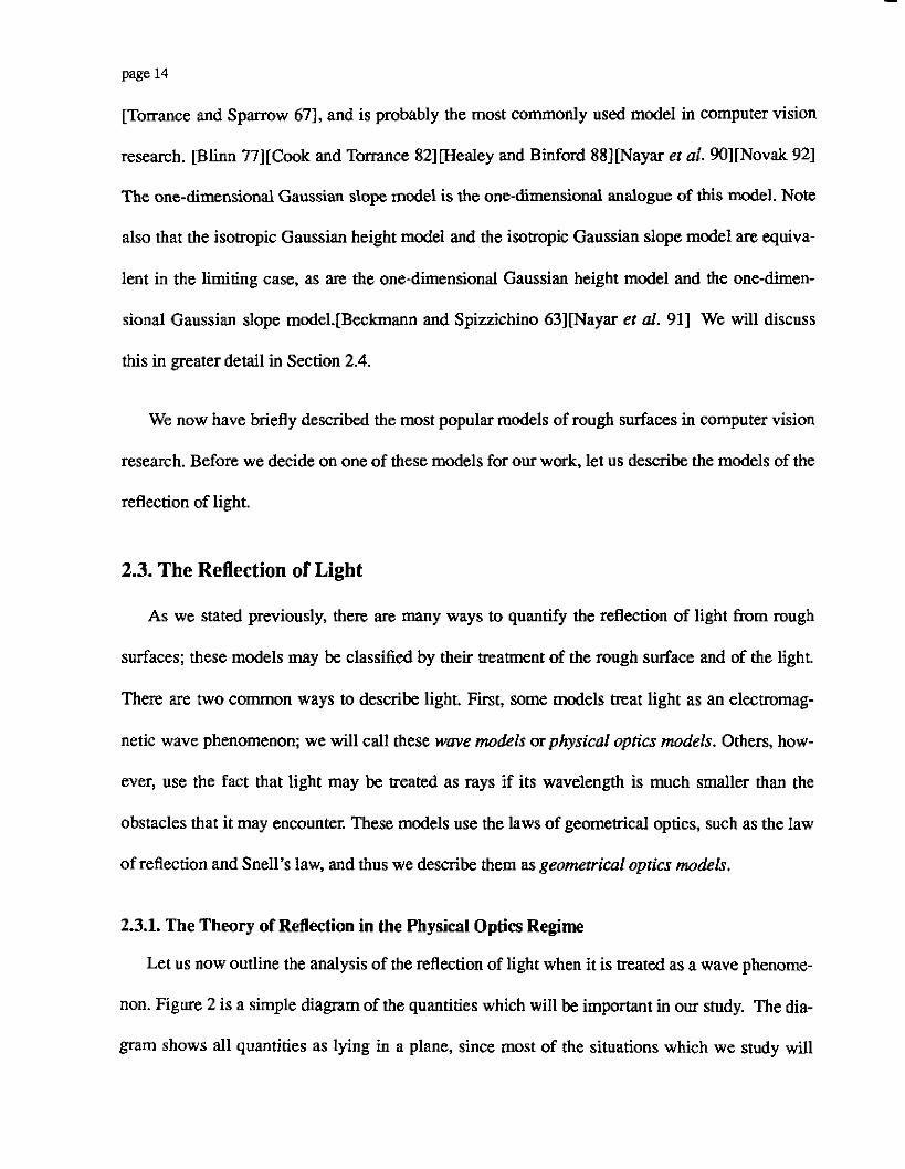
[Torrance and Sparrow 671, and is probably the most commonly used model in computer vision
research. [Blinn 77][Cook and Torrance 82lFealey and Binford 88NNayar et at. W][Novak 921
The one-dimensional Gaussian slope model is the one-dimensional analogue of this model. Note
also that the isotropic Gaussian height model and the isotropic Gaussian slope model are equiva-
lent in the limiting case, as are the one-dimensional Gaussian height model and the one-dimen-
sional Gaussian slope model.[Beckmann and Spizzichino 63][Nayar er d. 911 We will discuss
this in greater detail in Section 2.4.
We now have briefly described the most popular models of rough surfaces in computer vision
research. Before we decide on one of these models for our work, let us describe. the models of the
reflection of light.
2.3. The Reflection of Light
As we stated previously, there are many ways to quantify the reflection of light from rough
surfaces; these models may be classified by their treatment of the rough surface and of the light.
There are two common ways to describe light. First, some models treat light as an electromag-
netic wave phenomenon; we will call these wave models or physical optics models. Others, how-
ever, use the fact that light may be treated as rays if its wavelength is much smaller than the
obstacles that it may encounter. These models use the laws of geometrical optics, such as the law
of reflection and Snell’s law, and thus we describe them as geometricaloptics models.
2.3.1. The Theory of Reflection in the Physical Optics Regime
Let us now outline the analysis of the reflection of light when it is treated as a wave phenome-
non. Figure 2 is a simple diagram of the quantities which will be important in our study. The dia-
gram shows all quantities as lying in a plane, since most of the situations which we study will

Figure 2: The geometry for the scattering of light waves.
have scattering in the plane of incidence, and also because this makes the diagram easy to under-
stand. There are analogous results for scattering out of the plane which we will not show.
The direction of the incident light is denoted by the vector ki, and that of the reflected light by
k , . These vectors have magnitude equal to $, where h is the wavelength of the light. We will
assume for the moment that light is incident from only one direction, although it may reflect in
many directions, and hence, there will be many values of kr. The vector D is the scattering vector,
or kr - Ai, the difference between the reflected and incident vectors. Our goal is now to find the
intensity of the light for all directions of reflection, i.e. all values of k,, given the intensity and
direction of theincident light as well as the shape of the surface.
Because we are using the laws of physical optics, we treat the light as a wave. We solve for the
reflected intensity by treating each point of the surface as a point light source, and sum the effects

Page 16
of all sources, taking into account interference and diffraction. This is a difficult procedure, and
the results will vary greatly depending on the surface model that we choose. The most common
models used with the physical optics description of scattering are the Gaussian heights models,
both the one-dimensional and isotropic forms. Bec!unann and Spizzichino solved for the scattered
light intensity distribution for these cases and described the procedure for solving for the dishibu-
tion with the assumption of alternative surface models. Their derivation is too lengthy to include
here, but we present their result. The intensity, I, for a one-dimensionally rough surface with a
Gaussian distribution of height values is given by
X is the length of the part of the rough surface illuminated by the incident beam.
vx = (4) ( s iner+ sinei) and vz = k{mer- cmej) are the x and z components of the scattering
vector, respectively. g is equal to vzu , where a is the rms roughness of the surface. D is given by
: Corn tion and T is the correlation length of the surface. A definition of ngth appears with
the derivation. It is obvious that the expression is quite complicate& it is not surprising that it is
difficult to use in computer vision applications. This is especially true for intermediate values of
the roughness, i.e. g = 1, since the sum does not converge rapidly.
This formula is one of many that has been obtained for light scattering under the assumptions
of physical optics; it is also one of the simplest. Let us now see how this result compares with

page 17
those of the geometrical optics approach.
2.3.2. The theory of reflection in the geometrical optics regime
We may not only treat light as waves, but also as rays and thus describe its reflection and
refraction with the laws of geometrical optics. In this case, however, we ignore all diffractive
effects, and this is equivalent to the assumption that all obstacles that the light encounters are
much larger than its wavelength. For such obstacles, our calculated intensity distribution will be
correct, but for sufaces which have roughness on a scale much smaller than the wavelength of the
incident light, the calculated intensity distribution will be only an approximation to the true inten-
sity distribution.
Let us now describe the reflection of light from a rough surface with the methods of geometri-
cal optics. We first note that since we will be using the law of reflection, it is easiest to imagine
that the surface is comprised of small facets which reflect like a mirror. Figure 3 is a diagram of
such a surface. Once again, these facets are larger than the wavelength of the incident light. Since
the angle at which these facets are tilted will affect the reflection of light, we will use slope-based
surface roughness models. It is important to remember that, although we show the rays of light
reflecting off single facets in Figure 3, slope-based models do not deal with the individual facets
on the surface, but rather the statistical properties of the set of all facets on the surface.
We must now derive the radiance of light reflected by a rough faceted surface. This derivation
parallels that given by Torrance and Sparrow uorrance and Sparrow 671. Consider a small planar
patch of the surface under study, of size dA (see Figure 4). Assume an infinitesimal source of
radiance Li subtending a solid angle doi with direction of incidence, in spherical coordinates,
(e?qJ. (The normal to the mean surface is in direction (0.0). The reflected radiance is dr, with

page 18
Figure 3: A rough surface comprised of mirror-like facets. Light reflects off the facets according to the laws of geometrical optics.
*"f
______._._..----.-..- :--.-..-.-.------ ax
macroscopic surface normal
Figure 4: The reflection geometry for the derivation d t h e scattered light intensity, under the assumption of geometrical optics models.
page 19
direction (e,,@. For a given incidence direction and reflectance direction only those facets whose
normals bisect the angle between these directions will be able to reflect light from the source to
the receiver. Let the direction of the normals to these facets be (e,,q>. Let us denote the local angle
of incidence, or the angle between the source direction and the direction of the normals to the
privileged facets, as e iL.
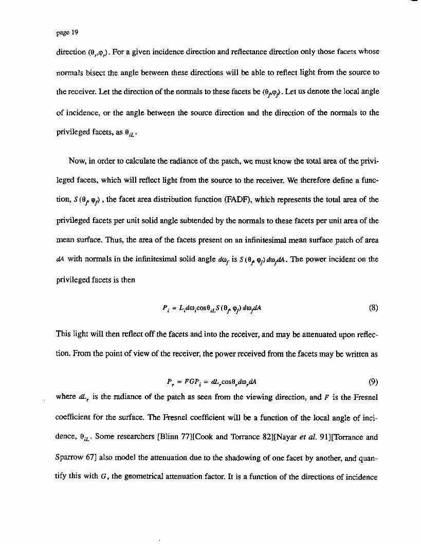
Now, in order to calculate the radiance of the patch, we must know the total area of the privi-
leged facets, which will reflect light from the source to the receiver. We therefore define a func-
tion, S (ef q) , the facet area distribution function (FADF), which represents the total area of the
privileged facets per unit solid angle subtended by the normals to these facets per unit area of the
mean surface. Thus, the area of the facets present on an infinitesimal mean surface patch of area
dA with normals in the infinitesimal solid angle do+ is s (e, ' p f )dm/4 . The power incident on the
privileged facets is then
This light will then reflect off the facets and into the receiver, and may be attenuated upon reflec-
tion. From the point of view of the receiver, the power received from the facets may be written as
Pr = FGP, = dLrcosB,dW,d4 (9) where dL, is the radiance of the patch as Seen from the viewing direction, and F is the Fresnel
coefficient for the surface. The Fresnel coefficient will be a function of the local angle of inci-
dence, eiL. Some researchers [Blinn 771[Cook and Torrance 82][Nayar et al. 91][Torrance and
Sparrow 671 also model the attenuation due to the shadowing of one facet by another, and quan-
tify this with G , the geometrical attenuation factor. It is a function of the directions of incidence

page 20
and reflectance. Torrance and Sparrow provide a derivation of this factor. Substituting the expres-
sion for the incident power into equation (9), we see that the radiance of the surface patch is
Most researchers use the simplifying relation [Nayar er d. 91][Torrance and Sparrow 671
We, however, will most often use the relation
doli = dw, (12)
This is merely a statement of the fact that if we hold er constant, all the facets which may reflect
light from the source to receiver will have the same normal, and will reflect light in a specular
fashion, so that the incident and reflected solid angles will be equal. We have found that numerical
methods of calculating the reflected radiance often perform better if we use this relation. Addi-
tionally, the equation for the reflected radiance, which we will show presently, has the Same form
for both the one-dimensional and two-dimensional cases if we make this substitution.
For an extended source, the reflected radiance is then
where the integral is over the hemisphere for which 0, is less than a/2.
There is also a normalization condition which any realistic FADF must satisfy. Consider one
facet of the surface and let its area be dF. The area of the projection of this element onto the mean

If we were to add up all the projected areas of all facets on the surface, we would obtain dA, the
area of the patch, i.e.
We also know that
so that
and
which is the normalization condition.
Just as we were able to apply physical optics methods of scattering analysis to many types of
surface models, we may also apply the geometrical optics methods to many models. In fact, the
above results p a i n to any slope-based model, or FADE Perhaps the most commonly used slope-
based model, and perhaps also the most commonly used rough surface reflection model in com-
puter vision work, is that proposed by Torrance and Sparrow [Torrance and Sparrow 671. The
model assumes a Gaussian dismbution of facet normals, such that

The constant, c , is related to the spread of the distibution of facet normals. The model is isotro-
pic, and is hence independent of Qf.
2.4. Our Choice of Model
In much of our subsequent research, we will need to decide whether we want to analyze scat-
tering with the methods of physical optics or geometrical optics, and we will also require a model
of the rough surfaces we study. Ideally, we would like to find a way to combine the power of the
physical optics approach with the mathematical simplicity of the geometrical optics methodology.
There exist cases in which scattering may be described equivalently by the physical optics
approach and a certain height model for the surface, and by the geometrical optics approach and a
certain FADE Beckmann and Spizzichino have shown [Beckmann and Spizzichino 631 that for
surfaces with Gaussian height distributions where the rms height is much larger than the wave-
length of the incident light, equation (7) reduces to
where 1 is a constant which simply represents the radiance of the source. In other words, the scat-
tered radiance consists of two terms, the first of which is focussed in a narrow range of angles, and
which may only be derived by physical optics methods, and the second of which is equivalent to
geomenical optics scattering. Nayar Wayar et al. 911 calls the first component the “specular spike
component of reflection”, and the second, the “specular lobe component”. It is interesting to note
that the first term is the same as the diffracted radiance distribution resulting from a single-slit

Page 23
source. The second term of equation (17) may be modified to include the effects of the Fresnel
coefficient and the shadowing of one facet by another as was done in equation (13). This yields
For a surface with a one-dimensional Gaussian height dismbution, the FADF is
and for a surface with an isotropic Gaussian height distribution, the FADF is
In these functions, p is the roughness parameter, and the rms slope, i.e. --? standard L-viation
of the facet slopes, is p/& for the one dimensional case and p for the isotropic cases. As noted by
Beckmann and Spizzichino and Nayar, these functions may be approximated by Gaussians in the
limit of small p , and thus the model of Torrance and Sparrow is a reasonable approximation to
equation (20) in this limit. It is interesting to note that in one sense such a surface is smooth, since
p is small and the surface has only low slopes, yet in another sense, the surface is rough, since the
rms height is much larger than the wavelength of light. The above facet area distribution functions
are more realistic than the Gaussian models, however, since they satisfy the normalization condi-
tion (equation (15)). We will use equations (17) and (19) in most of our work.

page 24
2.5. Conclusions
In this chapter, we have taken a brief look at a few of the many ways of modelling rough SUT-
faces and the reflection of light from them. We described both the height-based and slope-bas&
models for rough surfaces, and presented a normalization condition for a l l slope-based models, or
Facet Area Distribution Functions. We noted that the two methods of describing light reflection,
the physical optics approach and the geometrical optics approach, each have their strong points;
the physical optics models yield very accurate results, while the geometrical optics models are
easier to use. In order to combine the good points of both approaches, we will use the model of
Beckmann and Spizzichino, which is derived using physical optics methods, but which has a geo-
metrical optics formulation for the limiting case of rough surfaces. We must now use this model to
calculate the effects of roughness on the reflected images of step edges.
3. Edges
3.1. Chapter Overview
We saw in Chapter 2. that the mo-.. 2 Beckmann an Spizzic in0 provides a powerful, yet
easy-to-use, method of describing rough surfaces and the reflection of light from them. In this
chapter, we calculate the appearance of the image of a reflected step edge, assuming this model.
We then show how the shape of the edge varies with respect to changes in the roughness, the dis-
tance between the source and object, and the viewing angle. Following this is a discussion of how
different sets of these parameters may produce reflected edge images which are almost indistin-
guishable. We therefore conclude that knowledge of the source-object distance and viewing angle
is necessary for the functioning of any roughness estimation method which relies on the analysis
of edges.
3.2. Edges as an Extended Source
As we stated in Chapter 2., we will study the images of edges reflected in rough surfaces. Let
us begin this study by first defining a bit of our terminology. It should be clear from context when
we use the word edge to refer to the physical edge of the s o m e and when we use it to refer to the
reflected image of the source. We will try to be. clear in our usage, nonetheless, and will use terms
like reflected edge image and image of the refIecrion of the edge whenever possible. The reflected
image of the source will occupy a large part of the images we study. In order to make our results
easier to understand, we will therefore often show plots of the intesity of the reflected edge image
along the direction perpendicular to the image of the edge of the source. We will call these plots
reflected edge profiles. Now, let us describe the physical step edge source as an extended source
so that we may use equation (1 8) to calculate the appearance of the reflected image.
Page 26
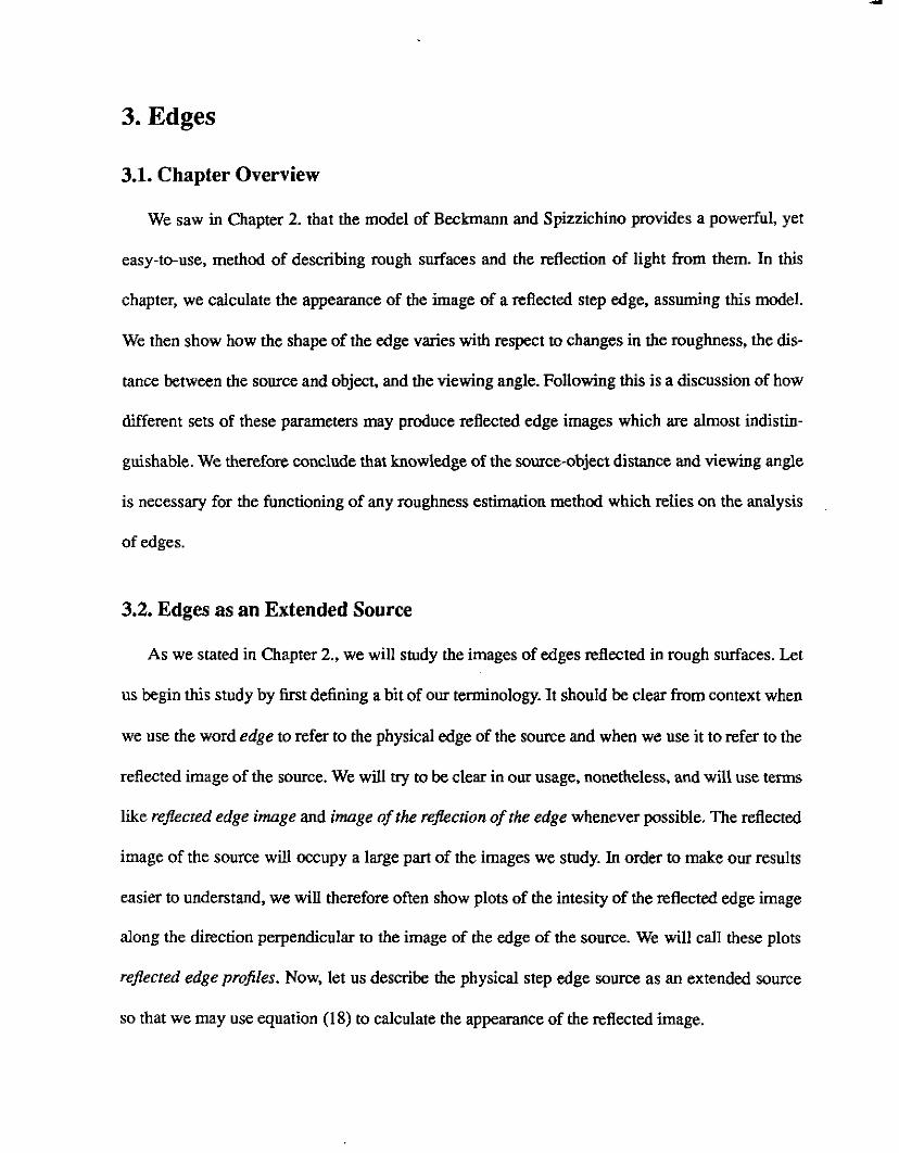
Consider a small patch of the reflective surface; perhaps it is the area viewed by one pixel.
The illuminutiun envirunmenrof this patch is the incident radiance for each incident direction, i.e.,
the brightness seen at the patch in each direction. Now let us assume that there is a step edge
which can be seen reflected in the surface. The illumination environment will thus contain a
bright region and a dark region. As we move from point to point on this surface, the two regions
which define the step edge will change, and thus, so will the illumination environment. As an
example, Figure. 5 shows the hemisphere of possible directions of incident light for several points
on a surface; the shaded regions show the directions from which light does impinge upon the sur-
face. This type of diagram is similar to the illustrations in [Maxwell and Shafer 931.
camera Q illumination environment at point A
A
C
Figure 5: The illumination environment for several points on a surface. The shaded regions d t h e hemispheres shaw the
angles from which light is incident on the surface.
page 27
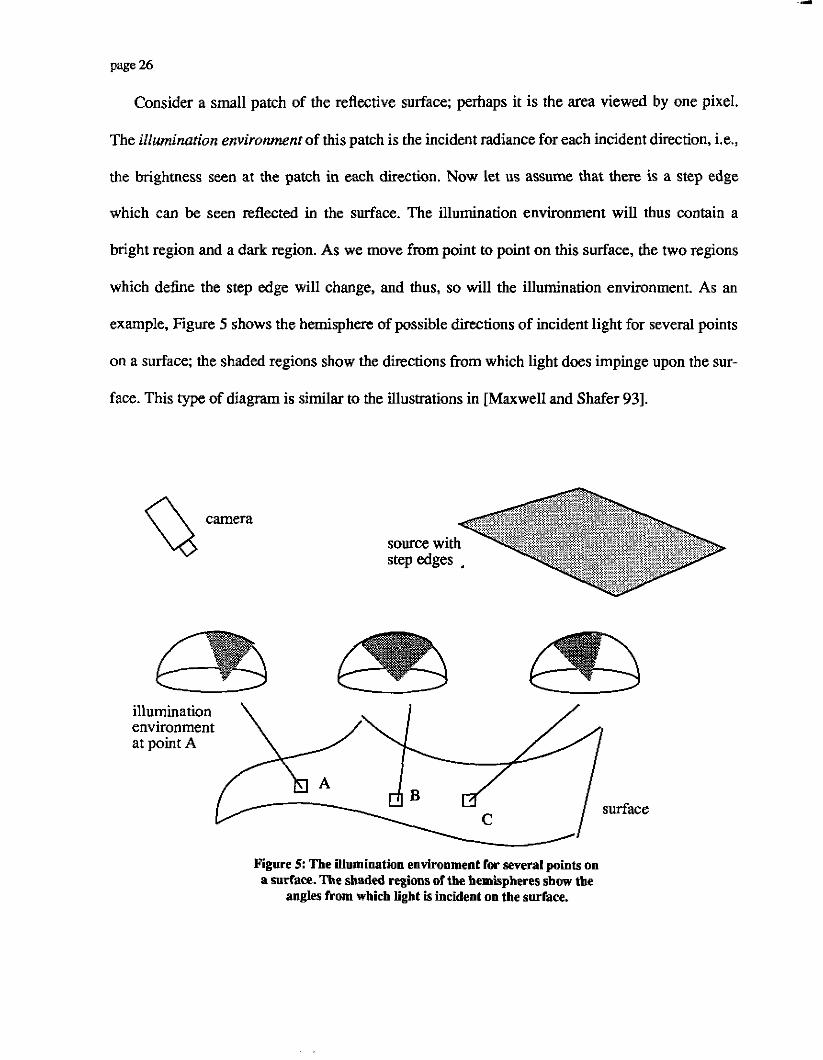
In most of this research, we will focus on one-dimensionally rough surfaces. The illumination
environment containing a step edge is particularly simple for this case. We will perform our calcu-
lations in the coordinate system of the surface patch. Therefore, let the normal to the patch be
along the z-axis, as shown in Figure 6, and let the grooves lie parallel to the y-axis (Le. the height
is constant for constant x). To begin, let us first consider the easiest case, in which the view vector
lies in the plane of the surface normals, i.e., the x-z plane, and assume the edge of the source is
parallel to the y-axis. As we see in Figure 7, light may be incident on the surface at many angles,
ei, where -5 < ei < !! . We assume that the illumination environment consists of a step edge of con- 2- 2
stant radiance, i , and thus, L, equals I for Oio s e i s O i l , and zero otherwise. We also know the
direction of the view vector, and hence 8,. for the patch. Because the facets which reflect light
from the source to the camera bisect the angle between these dmtions, we have
A macroscopic j surfacenormal
bisector of d"f *f Q
t ._._____..-.-----
Figure 6: The reflection geometry.
and reflection
t z
Figure 6: The reflection geometry.

x
Figure 7: The one-dimensional reflection geometq
ei+ e? ej =
and we therefore know the range of values of e, for which light will reflect from the source into
the camera. Let us denote the starting and ending values of this range by ep and eP, where
and e,-, = - eil + er . We are now able to calculate the reflected radiance for the surface 'io + Or 2
efl =
patch.
Before we do this, however, we note that eio and O i l , and hence the values of OD and en, vary
from point to point on the surface because the source subtends a different angle at each point. In
order to find the form of the reflected image of the edge, we must know the values of efl and ejl
at every patch on the surface. These values will depend on the relative positions of the source and
surface; for instance, for a source which is far from the reflective object, en and e,-, will vary

page 29
slowly across the surface while they will change much more quickly across the surface for a
source that is closer to the object. Similarly, e, will be different for different points on the surface,
and it depends on the relative positions of the reflective object and the camera. All of these vari-
ables depend on the shape of the object. To sum up, em, O f l , and 8, are all functions of the posi-
tion on the object, x . We denote this by e,&), ef l (x) , and O,(x). We also note that it is possible for
the radiance pattern of the incident light to vary from point to point on the reflective surface. This
will be true if the source radiance depends on the direction from which the light leaves the source.
Most light bulbs exhibit this behavior, as do many materials which act as sources by reflecting
light. However, if the distance from the surface to the source is much larger than the length of the
surface under study, the radiance pattern of the incident light will change little across the reflec-
tive surface, since the angles subtended by the source change little over this length. Even in cases
where the source is relatively close to the surface, we will assume that the source is Lambertian,
that is, its radiance is independent of the direction of the emitted light. We do this in order to be
able to calculate the reflected radiance pattern.
Now, let us return to equation (18), which gives the reflected ladiance for a patch. Once again,
it is
or, for an extended source
We will make the simplifying assumptions that F = 1 and G = 1. The fust assumption holds

page 30
fairly well over a large range of angles for most metals. The second assumption holds when both
ei and e7 are less than approximately 45 degrees[Nayar et al. 911. With these assumptions and the
one-dimensional form of the FADF given by equation (19), the equation for the reflected radiance
becomes
Let us now focus on finding the integral of the second term in this equation. Because the angle
at which light is incident on each facet must equal the angle at which light exits the facet,
and thus
and
If we remove the assumptions that the edge of the source is parallel to the grooves of the
rough reflecting surface and the view vector lies in the x-z plane, we only modify the quation

.-
page 31
slightly. Note that the rough surface is still parameterized by a single variable, Or, so that we may
still calculate the reflected radiance by means of equation (24). For this case, however, coseiL is
given by
Because the surface is "one-dimensionally" rough, however, 'pf = 0, and thus
so that
In order to complete this description of the reflection of light from rough surfaces, we must
calculate the integral of the first term in equation (28), the specular spike component. As stated in
Chapter 2., vx is the x-component of the scattering vector, or
p = (4) (sine, + sinej)
Therefore, the specular spike component of reflection is
where k is the wavenumber of the light, or 2r divided by the wavelength. Figure 8 shows the cen-

X
Figure 8: The central lobe of the square of the anc function and a Gaussian of approximately the
same width.
tral lobe of this function and a Gaussian with a similar width. It is obvious that we may approxi-
mate the spike component with a Gaussian with minimal loss of accuracy. This fact was first
noted by Nayar[Nayar er al. 911. Therefore, we model the radiance of the spike component as.
where we have set X equal to L, and 5 is the cross-sectional length of the incident beam. If 5
remains constant, the length of the illuminated portion of the surface will change in this fashion.
By equation (21), we may write
m e r

page 33
where we may make the final approximation because, as we stated in Section 2.4., the specular
spike component is focused in a narrow range of angles and thus has non-zero radiance only for
small values of ef Thus, for a point source, the reflected radiance of the spike component is
where we now let a quantify the angular spread of the spike component. We expect that a will
remain constant with respect to roughness, since this has no effect on the wavelength of the inci-
dent light or the effective beamwidth. For a step edge, the reflected radiance of the specular spike
component is
We now substitute this expression into equation (28) and find the equation for the radiance of light
reflected from a rough surface to be
In our experiments with rough surfaces and roughness estimation algorithms, we find that the
ratio of the radiances of the two components of reflection does not always behave as predicted by
equation (33). We therefore allow the magnitudes of the two components to vary independently in
our algorithms. This is probably an over-generalization of the reflected radiance equation, since

page 34
there appears to be some relationship between the two radiances, but since we do not how the
form of this relationship, we assume their independence. We thus model the radiance of the
reflected light as
where we have introduced A and E to describe the magnitudes of the two components. Any
changes in the multiplicative constant I can be equivalently modelled by changes in A and E , and
therefore, 1 no longer appears in the equation. Further discussion of the behavior of the relative
radiances of the specular spike and specular lobe components appears in Chapter 4.
Equation (34) allows us to calculate the radiance of the reflected edge image at any point on
the rough reflective surface. The behavior of this equation with respect to its parameters, such as
the roughness and the viewing angle, determines how much information we may obtain from the
reflected image. For example, if the fonn of a reflected edge varies little with respect to rough-
ness, then no method of roughness estimation based on edge analysis will work. Therefore, let us
investigate the behavim of this equation, so that we may develop realistic methods of roughness
estimation.
3.3. Limitations on the Differentiation of Edges
We may now use equation (34) to predict the appearance of edges under a variety of condi-
tions: different roughnesses, different object shapes, and different souroe, object, and camera con-
figurations. We want, however, to be able to solve the inverse problem, that is, given the

Page 35
appearance of the edge, find the roughness of the object. The measured appearance of the edge,
including the effects of noise and finite image size, will obviously af€ect our ability to determine
the roughness. We will attempt to quantify such limitations. To do this, we will simulate the
appearance of reflected edges for different roughnesses and different source, object, and camera
configurations. If we find that for a particular configuration the reflected edge image does not
change with respect to roughness, then we conclude that for this configuration, no information on
the roughness of the surface may be obtained.
3.3.1. Source-Object-Camera Configuration for the Simulations
We will begin by studying same edge profiles for the simple case in which the reflective sur-
face is planar, and the source is an infinite half plane parallel to the reflective surface. Figure 9 is a
schematic of this configuration. We also assume that the camera is far from the surface, so that
top view front left view
reflective object
I source source
camera Figure 9: Schematic of the simulation configuration

page 36
is approximately constant across the region of interest of the surface. In our simulations, the
parameters of this configuration which we will change are the surface roughness, the perpendicu-
lar distance between the plane of the source and the plane of the reflective surface, and the view-
ing angle.
We choose this arrangement of s o m , object, and camera for several reasons. First, this is
essentially the configuration that will be used in our later experiments. Therefore, any insight we
gain from these simulations can be applied to our experiments. Secondly, the assumption of a pla-
nar surface allows us to ignore the effects of the object curvature on the appearance of the edge.
This will make OUT initial set of simulations easier to understand. We will discuss the effects of
surface curvature on reflected edge profiles briefly at the end of the chapter.
The choice of an infinite half-plane serves several purposes. Note. that equation (34), the
expression for the reflected radiance, is a difFerence between two similar terms, one dependent on
the variable On, which describes the angular position of one side of the bright region in the illumi-
nation environment, and another term dependent on the variable On, which gives the position of
the other side of the bright region. Thus, equation (34) actually represents the difference of the
two edges which bound the bright region in the illumination environment. If we allow our source
to be an infinite half plane, we essentially force en to go to -;, and we will be able to study the
appearance of a single edge. The closeness of the source serves another purpose. The values of efl
will vary from point to point on the reflective surface, while the values of Or will not change
much. Note that the error function terms in equation (34), which are the dominant terms, are sym-
metric with respect to ei, and er by equation (21). Thus, if the source were far from the object,
page 37
and the viewer near, it would be possible to obtain the same reflected edge image as with the
opposite configuration. We would also see the same changes in the appearance of the edge with
respect to changes in Or as we did in theopposite case with respect to changes in erl . Thus, this
initial set of simulations will be applicable to the case with the near camera and far source, as long
as we are careful to reverse the roles of the variables.
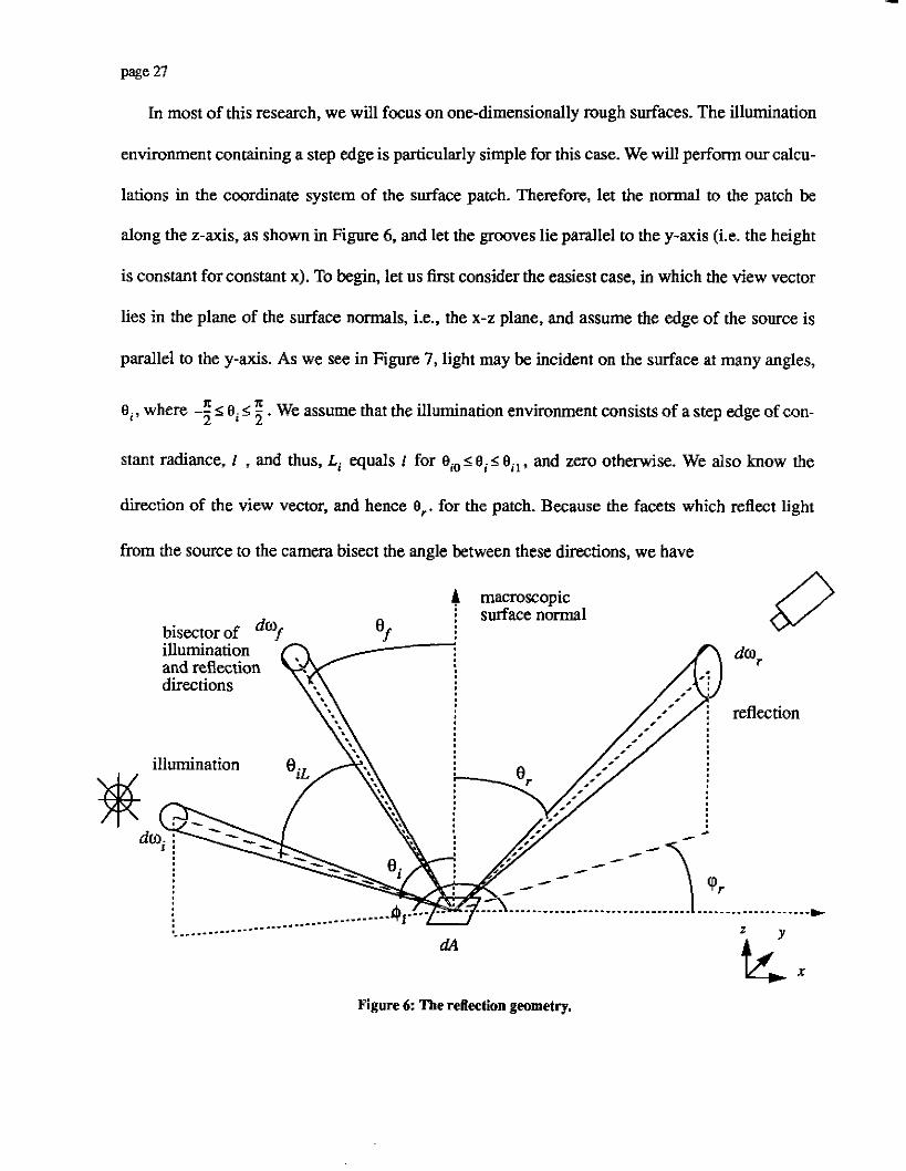
Figure 10 is the fmt example of our sets of simulated edge profiles, and shows the intensity of
the edge as a function of position along the surfm. It shows five profiles graphed together to
facilitate comparison. We choose the scale in these graphs to reflect the values in common imag-
ing situations. Our camera records intensity values in the range from 0 to 4095, and in order to
prevent clipping, we try to keep the maximum measured intensity in the range from 3000 to 4OOO.
For this series of simulations, the values of the parameters in equation (34) are
1500.00
5m00
--.- beta - 0.20 beta - 0.15 beta = 0.1 0 beta - 0.05
--- -.- .._ ...... - beta - 0.0
X Figure 10: Edges far several values of beta. As the roughness
inereass, the top and bottom of the edge k a m e mare rounded. A = 1O00, B = 1000,0, = O b degrees,D = 500, a = 0.0.

page 38
0 A - the magnitude of the specular spike component, intensity units
B - the magnitude of the specular lobe component, lo00 intensity units
- 9, - the viewing angle, 0 degrees
- D - the source to surface distance, 500 length units
a - the width of the specular spike component, 0.0. For this value of a, the specular
spike component becomes a delta function.
p, therms slope, takes on the values 0.00,0.025,0.050,0.075, and 0.100. As expected, the higher
the value of PI or the rougher the surface, the more the lobe component spreads out, and the more
rounded the top and bottom of the edge profile become. Let us now change the values of the
parameters, and see what effects this will have on the edge profiles.
3.3.2. The Effect of Changes in the Source-Object Distance
Consider equation (34) once again. The variable gives the angle of the normal to those fac-
ets which will reflect light from the edge of the source into the camera. The functional form of efl
across the surface, ef l (x) ,largely determines the appearance of the reflected edge. For our simula-
tions, with a planar surface, parallel planar source, and distant camera, equation (21) yields
where D is the perpendicular distance between the source and surface, and the origin of the coor-
dinate system is at the point on the surface closest to the edge of the source. Figure 11 shows the
relationship between the angles.
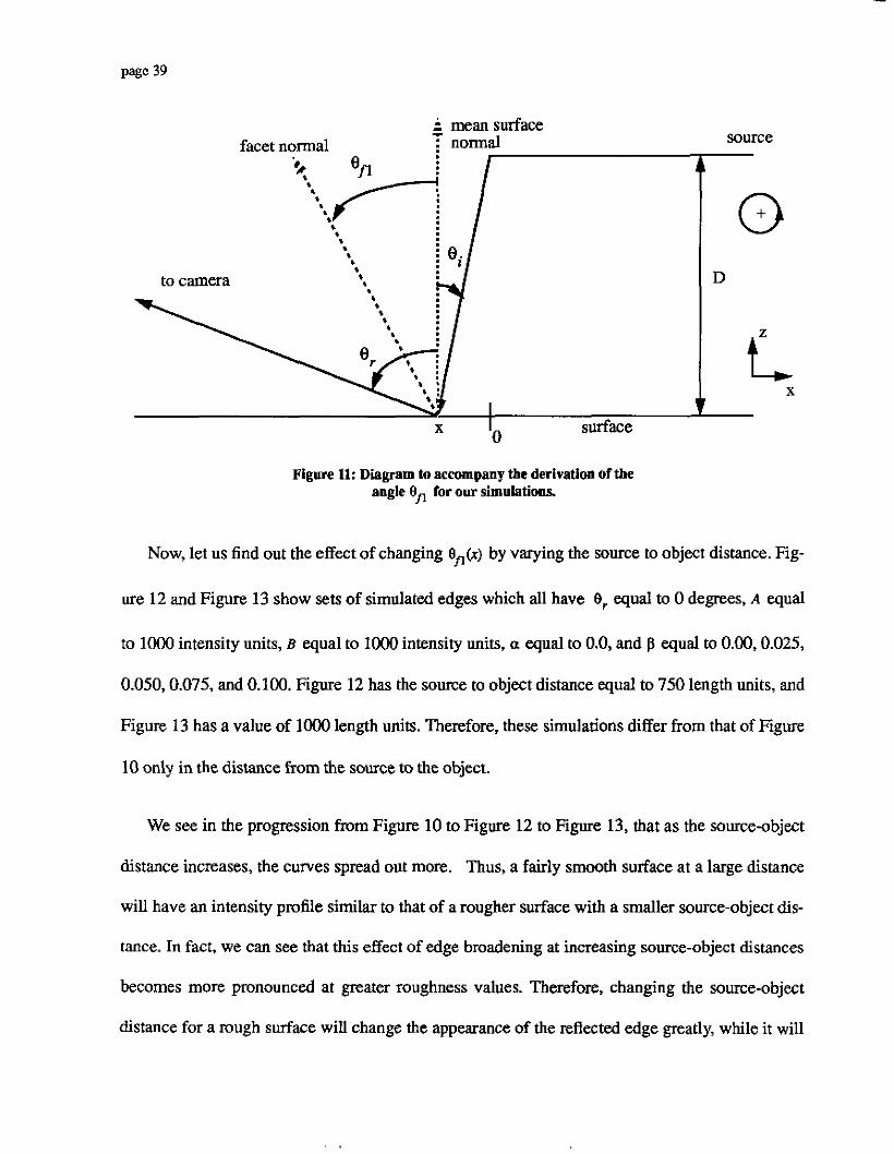
page 39
Figure 11: Diagram to accompany tbc derivation of the angle On for OUT simulatiws.
Now, let us find out the effect of changing On(x) by varying the source to object distance. Fig-
ure 12 and Figure 13 show sets of simulated edges which all have 0, equal to 0 degrees, A equal
to loo0 intensity units, B equal to IO00 intensity units, a equal to 0.0, and p equal to 0.00,0.025,
0.050,0.075, and 0.100. Figure 12 has the source to object distance equal to 750 length units, and
Figure 13 has a value of lo00 length units. Therefore, these simulations differ from that of Figure
10 only in the distance from the source to the object.
We see in the progression from Figure 10 to Figure 12 to Figure 13, that as the source-object
distance increases, the curves spread out more. Thus, a fairly smooth surface at a large distance
will have an intensity profile similar to that of a rougher surface with a smaller source-object dis-
tance. In fact, we can see that this effect of edge broadening at increasing source-object distances
becomes more pronounced at greater roughness values. Therefore, changing the source-object
distance for a rough surface will change the appearance of the reflected edge greatly, while it will

1 3m.00
0) E 2 s 2500.00
1m.00 -
500.00 -
0.00
- .. - beta - 0.20 - -- beta-0.15 -.- beta = 0.10 . . . . . . . . . beta - 0.05 - beta-0.0 *f ,2. / . .A, .
I
X
Figure 12: Edges for several values of beta, A = 1 W , B = 1000, er = 0.0 degrees D = 750, a = 0.0.
0 3ooo.00-
9!
* z 2500.00 -
2ooaw -
1500.w -
lwo.00 -
m . w ]
- .. - beta - 0.20 --- beta - 0.15 --- beta - 0.10 . . . . . . . -. beta = 0.05 - beta- 0.0
Figure 13: Edges for several values of beta. A t 1o00, B = 1000, Or = 0.0 degrees, D = 1O00, a = 0.0.

page 41
cause less of a change for a smoother surface, and a perfectly smooth surface appears the same at
all source-object distances. We conclude, therefore, that the distance between the source and
object planes drastically affects the reflected image of the edge. This is especially true the rougher
the surface.
3.3.3. The Effect of Changes in the Viewing Angle
Next, let us test the effect of changing er on the appearance of the edges. We expect to see
some change, since as we vary the viewing angle, different facets will reflect light from the source
into the camera. Everyday experience, however, indicates that there might not be a large amount
of change until er approaches grazing angles, since the appearance of images reflected in metals
tend to look the same for most viewing directions.
Figure 14 to Figure 16 show sets of simulated edge profiles which all have a source to object
distance of 750 units, A equal to intensity units, a equal to
0.0, and 9, equal to 0, 15, 30, and 45 degrees.. Figure 14 has p equal to 0.0, Figure 15 has p
intensity units, B equal to
equal to 0.05, and Figure 16 has p equal to 0.1. As expected, the curves with p equal to 0.0, i.e.
the profiles for a perfectly smooth surface, look the same for all angles 8,. For the other values of
p, the edge profiles broaden as we increase e,, although the effect is not as strong as in the simu-
lations in which we varied the source to object distance. Also, this broadening is greater for
greater roughness values. Another feature of these graphs is that for greater values of e?, the last
term of equation (34) becomes larger, and the lobe component changes slightly, but noticeably.
This results in the apparent asymmetry of the graphs, which is actually because of the slight
change in height of the lobe component.
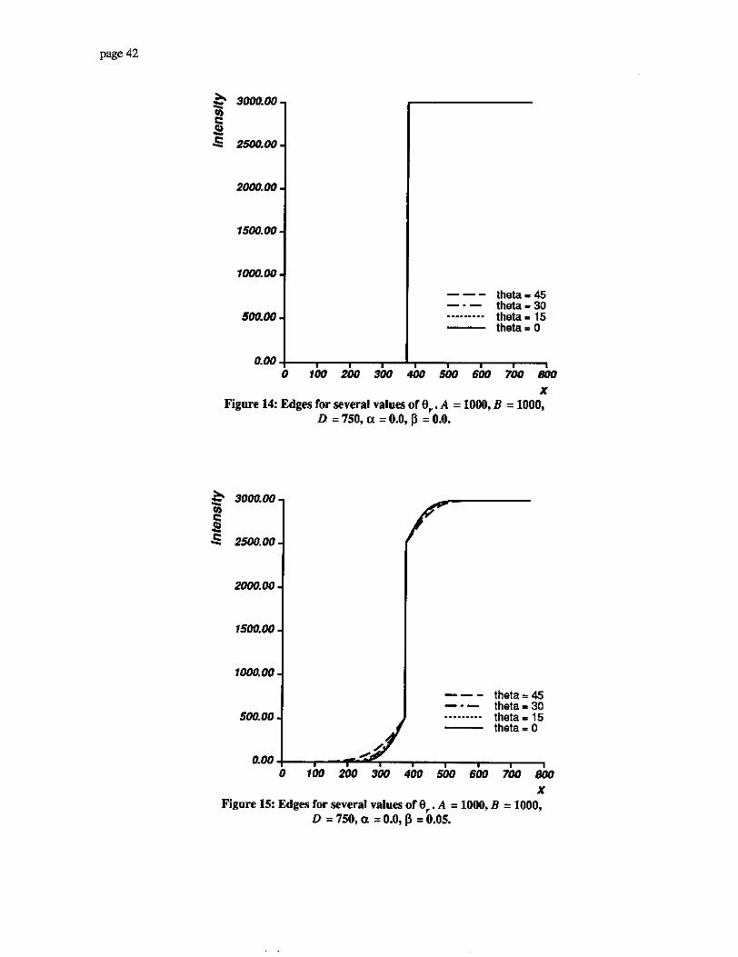
page 42
3 3 m 0 0 -
c % u)
s 2500.00-
2ooo.00 -
15oO.W -
I w o . 0 0 -
5oaw -
a. w
theta - 45
theta = 15
--- theta - 30 theta-0
-.- ......... - 1
0 100 200 3W 400 500 6W 700 800
theta = 45 theta - 30 theta - 15
--- -.- ......... - theta- 0
0.00 I 0 100 200 300 400 500 600 700 800
X Figure 15: Edges for several values of Br . A = 1000, B = 1000,
D = 750, a = 0.0, p = 0.05.

page 43
theta - 45 theta - 30 theta - 15 theta - 0
--- ....... _. -
X
Figure 16: Edges for several values of 0,. A = 1000, B = 1000, D = 750, a = 0.0, p = 0.10.
Our next conclusion is that the the viewing angle does indeed affect the shape of the reflected
edge profile, albeit not as drastically as did the source-object distance.
3.3.4. The Effect of Changes in the Specular Spike Width
For the sake of completeness, we must study a, which determines the width of the specular
spike component of reflection. The expression for the pan of the edge prolile due to the spike
component is quite similar to that due to the lobe component, so we expect it to spread with
increasing a,
Figure 17 shows edge profiles where the distance from the source to surface is 750 length
units, Or is 0 degrees, A is lo00 intensity units, B is loo0 intensity units, p is 0.05, and a takes on
the values 0.0, 0.015, and 0.030. The behavior is similar to that for a change of p, but, as
expected, it is now the spike component which spreads. According to our model, a has no depen-

aloha - 0.030 ._....... Y - ~ ~~~
-.,.1a-0.015 - alpha = 0.000
X Figure 17: Edges for several values of alpha. A = 1000, B = 1000,
€Ir = 0.0 degree& D = 750, fi = 0.05.
dence on other parameters such as
help us to determine if this is in fact hue.
fi, and the source to object distance. Our experiments will
3.3.5. Ambiguous Edges
We now have an idea how the intensity p f i l e across an edge varies as the roughness, viewing
angle, and source to object distance change.With this knowledge, we may point out some limita-
tions in the analysis of edges.
First, consider Figure 18. In it, we see two edge profiles. One of these has A equal to loo0
intensity units, B equal to lo00 units, a equal to 0.0, p equal to 0.10, Br equal to 0 degrees, and a
source to object distance of 750 length units. The other edge profile has A equal to 1oM3 intensity
units, B equal to lo00 units, a equal to 0.0, p equal to 0.15 , Or equal to 30 degrees, and a source
to object distance of 425 length units. Obviously, the surfaces and configurations are quite differ-
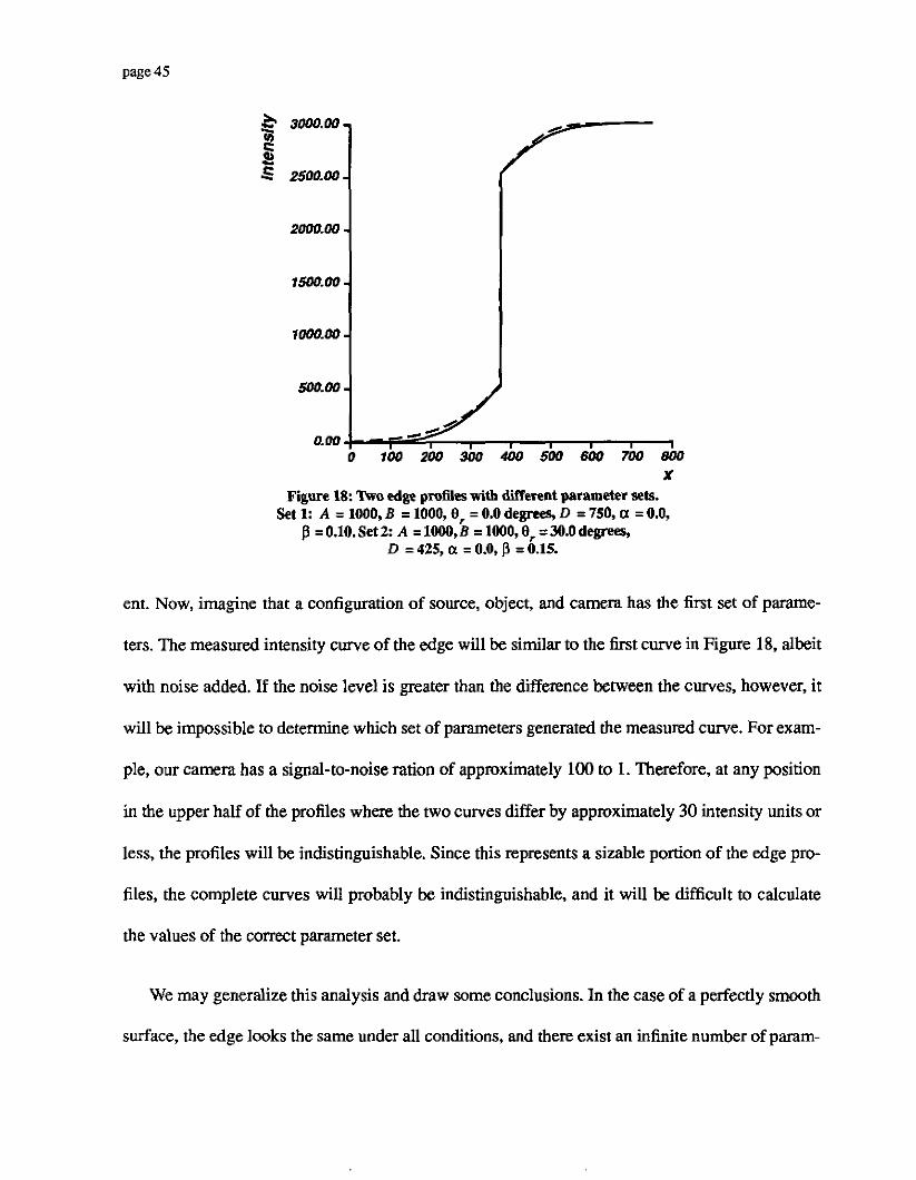
page 45
ent. Now, imagine that a configuration of source, object, and camera has the first set of parame-
ters. The measured intensity m e of the edge will be similar to the first curve in Figure 18, albeit
with noise added. If the noise level is greater than the difference between the curves, however, it
will be impossible to determine which set of parameters generated the measured curve. For exam-
ple, our camera has a signal-to-noise ration of approximately 100 to 1. Therefore, at any position
in the upper half of the profiles where the two curves differ by approximately 30 intensity units or
less, the profiles will be indistinguishable. Since this represents a sizable portion of the edge pro-
files, the complete curves will probably be indistinguishable, and it will be difficult to calculate
the values of the c a t parameter set.
We may generalize this analysis and draw some conclusions. In the case of a perfectly smooth
surface, the edge looks the same under all conditions, and there exist an infinite number of param-

page 6
eter sets which may generate the same edge profile. In this case, however, it is easy to determine
the roughness, p, which is of interest to us. For other values of the roughness, however, there exist
many parameter sets which may generate the same curve, to within noise levels, thus making any
analysis of the roughness suspect. Therefore, OUT first conclusion about the limitations of edge
analysis is that for any surface which is not perfectly smooth, the viewing angle and source to
object distance must be known in order to determine the surface roughness.
Next, consider Figure 19. One of these edges has A equal to IO00 intensity units, B equal to
IO00 units, a equal to 0.0, p equal to 0.15, er equal to 0 degrees, and a source to object distance
of 1O00 length units; the other has the same values for all parameters except p , which equals 0.20.
In Figure 13, these curves look significantly different, and yet, in Figure 19, their differences are
beta - 0.20 beta-0.15
. . . . . -. . .
0.00 I, 2611 280 500 320 340 360 380 4w 420 440 460 480
X Figure 1 9 Part of the edge profiles for beta equal to 0.15 and
0.20. A = 1000, E = 1000, Or = 0.0 degrees, D = 1000, a = 0.0.

page 41
small, in fact, the greatest difference between the curves is only about fifty intensity units. This is
obviously due to the fact that we only show part of the complete edge profile. If we attempt to
determine the roughness from one of these graphs, it will therefore be difficult to obtain an accu-
rate value for p . For a fixed image width, this effect is more pronounced at greater roughness val-
ues and greater source-object distances, since these widen the reflected image of the edge. There-
fore, our next conclusion about the limitations of edge analysis is that we should have the full
edge profile in order to accurately measure the roughness. Although this may seem to be a minor
point to make, the iruncation of the reflected image of the edge may easily occur in real imaging
environments.
3.4. The Effect of Surface Shape
We have seen how the image of a step edge reflected in a planar rough surface behaves with
respect to some-object distance, viewing angle, and roughness. Another variable which we have
not yet studied is the shape of the reflective surface. We will see that the effect of the object shape
on the reflected edge image is mostly a combination of the effects we have already studied.
Consider a generic surface. The position of a patch of the surface and its orientation are well-
defined, although they may take on any values. As we move across the surface, these two values
will change, and thus, so will the viewing angle, er , and the angle of the facets which reflect light
from the edge of the source, efl. With the proper placement and orientation of the patch, it is pos-
sible to obtain any value for the reflected radiance between zero and a maximum value which
must be less than or equal to the radiance of the source. The proper placement and orientation of
all patches on the surface can thus generate any given edge profile. Therefore, if we know the
position and orientation of all patches on the surface, we may use equation (34) to calculate the

page 48
appearance of the reflected image of a step edge for a given roughness and configuration of
source, object, and camera, or we may solve the inverse problem and calculate the roughness,
given the same knowledge about the configuration. If we do not know the shape of the reflective
object, however, such calculations ax impossible, since a given edge profile can result from a
multitude of configurations of source, camera, object position, and object shape. If we assume that
the surface is continuous, this limits the number of configurations which can produce the reflected
edge image, but not enough to produce a one-to-one mapping between edge profiles and surface
shapes. We therefore conclude that it is necessary to h o w the shape of the reflective object in
order to calculate the roughness of the surface.
The effect of the surface shape on the reflected edge image is even more complicated than this
analysis seems to imply. Curved mirrors may act as lenses, and they suffer from many of the same
distortions, such as spherical aberration and coma. Therefore, some blurring of the edge image
may be due to the shape of the surface, rather than the roughness. As a result, roughness estima-
tion algorithms will tend to calculate the value of the roughness as being greater than its true
value. Again, in order to account for such effects, the shape of the surface must be known.
Despite all of these difficulties, there are a few general statements that we can make about the
effect of surface shape on the behavior of reflected images of step edges. First, as long as the sur-
face curvature is small relative to the extent of the edge, we may approximate the surface as a
plane over the region of interest, and use the information we obtained in Section 3.3.. Secondly, if
the surface has a single sign of curvature, the width of the edge varies monotonically with respect
to the curvature. Consider Figure 20. Here we see a step edge and a convexly curved reflective
surface. The values of 0, and ei change more quickly with respect to x than they do for a plane,
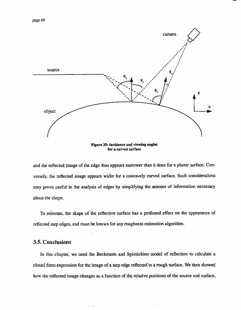
Figure 20: Incidence and viewing angles for a curved surface
and the reflected image of the edge thus appears narrower than it does for a planar surface. Con-
versely, the reflected image appears wider for a concavely curved surface. Such considerations
m y prove useful in the analysis of edges by simplifying the amount of information necessary
about the shape.
To reiterate, the shape of the reflective surface has a profound effect on the appearance of
reflected step edges, and must be known for any roughness estimation algorithm.
3.5. Conclusions
In this chapter, we used the BBckmann and Spizzichino model of reflection to calculate a
closed form expression for the image of a step edge reflected in a rough surface. We then showed
how the reflected image changes as a function of the relative positions of the source and surface,

page 50
the viewing angle, and the surface shape. From our simulations, we were able to draw several
conclusions. First, that in order to determine the roughness of a surface from the reflected images
of step edges, the shape of the surface as well as its position relative to the source and the camera
must be known. Additionally, the image should contain as much of the reflected edge profile as
possible in order to prevent the calculation of incorrect parameter sets and roughness values.
These limitations apply not only to the roughness estimation methods we present in this thesis,
but to any method based on reflected edge images. Let us keep these results in mind and present
our methods for roughness estimation.

4. An Iterative Roughness Estimation Method
4.1. Chapter Overview
In this chapter, we present an algorithm which calculates the roughness of a surface by itera-
tively fitting a curve to the reflected image of an edge with a gradient descent algorithm. We first
describe the algorithm, and then discuss five rough surfaces on which we test the algorithm. The
rms slopes of the surfaces are found by stylus profilometry, a conventional method of roughness
measurement. We then use our algorithm on the images of step edges reflected in the five samples
and compare the results of our method with those found with the profilometer. We find that our
method orders all of the surfaces correctly by roughness. We also conclude that although this
method ranks the surfaces well, it may not be applicable as a mensuration scheme.
4.2. The Algorithm
Our first algorithm is actually a quite obvious way of determining the roughness of a reflective
surface. It fits a cuwe described by our model to the profile of a real reflected edge; the value of
the m s slope which results in the best fit curve is then taken to be the rms slope of the surface.
This procedure is not as simple as it may first seem, and we want to discuss some of the h e r
points in its application.
Let us begin by returning to equation (M), the equation for the appearance of a reflected step
edge image under the assumption of the Beckmann and Spizzichino model of reflection. It is

..-
In order to use our roughness fitting algorithm, we must find the values of er0 and efl for all
points on the surface. These give the orientation of the normals to those facets which reflect light
from one edge of the source into the camera We already found these values for our simulations in
Section 3.3.2. Let us briefly repeat the derivation. Figure 21 shows the s o m e and reflective object
as well as a ray of light that leaves the source and reflects off the surface. Note that since we
assume that the camera is far from the surface, 9, is a constant for all points on the reflective sur-
. Cxss,) .. . source plane -.
A D
7
Figure 21: A schematic of the experimental configuration

PF 53
face. For our experimental configuration, which we describe more completely in Section 4.4.,
'p, = 0, and the plane of reflection is perpendicular to both the reflective surface and the edge of the
source, and we may derive all the necessary terms from Figure 22. Let xSrc be a point on the
source, and x be a point on the object. We see that
where D is the distance between the source plane and the object plane. Also, by equation (21),
Because we model the step edge as a half-infinite plane, €$, is equal to -; for all points on the
surface. If we let the position of the edge be the origin, i.e. xSrc = 0 at the edge,
Figure 22: The reflection geometry for the experimental configuration

atan( s) + e, 2 ep =
We therefore know the initial and final values of e, for all points on the object, and we may use
equation (35) to calculate the radiance of the reflected light.
Now, in order to fit the model to the data, we must account for several effects which change
the appearance of the reflected image, but which are not included in equation (35). First, note that
the dimmest parts of the image will not have a zero intensity, but rather, then will be a constant
offset due to ambient light and perhaps camera effects such as the dark current, which is the cur-
rent presenr in the CCD even when no light enters the camera. We model this with the constant, C.
Next, note that the value given for e, is the result of a measurement and is therefore not exact; the
same is true for Bi . Apart from the term me,, which is a small number for this experimental con-
figuration and which is multiplied by othw small numbers, e, and Bi only appear as part of their
sum. Therefore, we may model the errors in both Or and ei by replacing 0, with e, + A0 . The final
model for the reflected edge is then
where
am( g) + er + AO,
Of, = 2
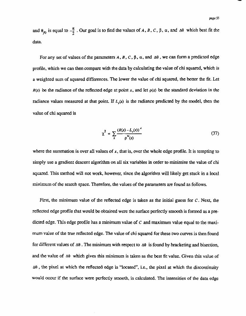
pl8e 55
and Bp is equal to -; . Our goal is to find the values of A , B, C, p, a , and AB which best fit the
data.
For any set of values of the parameters A , E , C, f3, a, and AB , we can form a predicted edge
profile, which we can then compare with the data by calculating the value of chi squared, which is
a weighted sum of squared differences. The lower the value of chi squared, the better the fit. Let
R(X) be the radiance of the reflected edge at point X , and let p(x) be the standard deviation in the
radiance values measured at that point. If L,(x) is the radiance predicted by the model, then the
value of chi squared is
where the summation is over all values of X , that is, over the whole edge profile. It is tempting to
simply use a gradient descent algorithm on all six variables in order to minimize the value of chi
squared. This method will not work, however, since the algorithm will likely get stuck in a local
minimum of the search space. Therefore, the values of the parameters are found as follows.
First, the minimum value of the reflected edge is taken as the initial guess for C. Next, the
reflected edge profile that would be obtained were the surface perfectly smooth is formed as a pre-
dicted edge. This edge profile has a minimum value of C and maximum value equal to the maxi-
mum value of the true reflected edge. The value of chi squared for these two curves is then found
for different values of AB . The minimum with respect to AB is found by bracketing and bisection,
and the value of A0 which gives this minimum is taken as the best fit value. Given this value of
At3 , the pixel a1 which the reflected edge is "located", Le., the pixel at which the discontinuity
would occur if the surface were perfectly smooth, is calculated. The intensities of the data edge

pmfde a few (usually three) pixels on either side of this pixel are recorded, and their difference is
taken as the initial value of A. The first guess for B is then the maximum value of the reflected
edge, minus C , minus A . Figure 23 shows a typical edges profile, and the initial values for these
parameters.
At this point, the initial guesses for A , B , C , and A8 have been determined, and the iterative
search for the best fit parameters begins. A gradient descent algorithm finds the value of beta
which minimizes chi squared for these initial values of A , B , Cand A8 , with a equal to 0.0. Beta
starts at 0.1; we choose this value because it seems to be in the middle of the range of p for com-
mon objects, and the algorithm converges well when starting from this value. When this gradient
descent subroutine reaches its minimum, p is held fixed, and the minimum with respect to a is
found by gradient descent. When this reaches a minimum, singular value decomposition is used to
X Figure 23: The initial guesses for the parameters A , B , and C for an edge
profile. The value of AB is related to the position ofthe edge.

m e 9
find the best fit values of A , B , and C for these values of p and a. The algorithm cycles between
fitting for p , for a, and for A , E , and C until convergence is reached.
In this section, we have presented an algorithm which utilizes both gradient descent and sin-
gular value decomposition to estimate the roughness of reflective surfaces. The algorithm uses a
model with six parameters: A and B , the magnitudes of the specular spike and specular lobe com-
ponents of reflection, respectively, C , the offset of the edge profile, p. therms slope of the surface,
a, the width of the specular spike component of reflection, and AB , the sum of the error in the
measurement of the viewing angle and the angle of incidence. The algorithm finds the values of
the six parameters which best fit the measured reflected edge image in the least-squares sense. Let
us now describe the results of using this algorithm on real images and surfaces.
4.3. The Surfaces
In order to test the accuracy of our methai of roughness estimation, we had to determine if
our calculated roughness values corresponded to those found by conventional means. This acted
as a test of the appropriateness of the method as a mensuration scheme. Therefore, we measured
our samples with a stylus profilometer, so that we could compare these measurements with those
made with our algorithm. In this section, we describe these measurements, and we also discuss
the validity of our assumption that the surfaces have a Gaussian distribution of height values,
which allowed us to determine if the distribution of height values affected the reflected edge pro-
file.
4.3.1. Height and Slope Statistics
In our experiments, we used samples of reflective surfaces with known roughness values. Our
samples were circular steel disks, three inches in diameter, which had been milled to produce a

one-dimensionally rough surface on one face of each disk. The values of the arithmetic average
roughness, R,, as stated by the manufacturer, were 1.5, 3.0, 4.5, 7.5, and 9.5 microinches.[Alcoa
941 As we mentioned in Chapter 2., the rms height and nns slope determine the distribution of
the scattered light more than do other surface statistics such as arithmetic average rough-
ness.[Beckmann and Spizzichino 63][Stover SO] Therefore, we could not use the roughness val-
ues stated by the manufacturer, but instead calculated the rms slopes of the surfaces from
measurements made with a profdometer.
Before we describe our measurements, we mention a caveat. As noted by Bennett and Matt-
son [Bennett and Mattson 891, different values of surface roughness will be obtained for the same
surface with different instruments. For example, stylus profilometers generally measure higher
values for the roughness of a surface than do optical profilometers. Keeping this in mind, we per-
formed the following measurements. A Tencor Alpha Step 200 stylus proflometer was used to
measure the surface profiles of the samples. For each scan, the profilometer measured the surface
height at 2000 points over a 400 micrometer distance, and ten scans were made for each sample.
We used these measurements to calculate the root-mean-square heights of the surfaces. The
calculated rms height values appear in Table 1. The values in microinches are given for compari-
son with the stated roughness values. Remember that the roughness values stated by the manufac-
turer were the arithmetic average roughness, rather than the root mean square roughness, and
therefore need not be the same as the values we calculate. Notice the unusually high value for the
7.5 microinches roughness sample; also note that the rms values place the samples in the same
order as do the arithmetic average roughness values.
Our edge fitting algorithm produces estimates of the standard deviation of the facets normals,

Measured rms roughness value
rms roughness micrometers microinches sample
1.5 microinches 0.0366 f 0.0002 1 . 4 4
3.0 microinches 0.0690 f 0.0003 2.72
4.5 microinches 0.136f0.001 5 .34
7.5 microinches 0.241 * 0.001 9 . 4 8
9.5 microinches 0.255 f 0.001 10.05
Table 1
rather than ms height values. In mst cases, it is difficult to relate these two parameters, but for a
surface with a Gaussian dismbution of heights, we know that the facet area distribution function
for such a surface is [Beckmann and Spizzichino 631
where CT is the rms height and T the correlation length of the surface. Comparison with equation
(19) shows that B = $. In order to find the correlation length of a surface with N height samples
at positions xi, we form the autocorrelation function,

where A is the spacing between the height sample positions, and ‘T = jA. This function should
have a maximum at T~ = 0. The correlation length, T, is defined as the position where the autocoT-
relation function reaches e -1 . hmes its peak value.
The correlation lengths of the surfaces were found by computing the autocorrelation function
of each profile, and then fitting a function of the form
in the least squares sense to each. The correlation length was found from this fitted function. The
resulting values appear in Table 2. Again, notice the large value for the 7.5 microinches roughness
sample. Graphs of the scans from the profilometer confmn that this sample has a high amplitude,
long wavelength variation imposed on the surface in addition to the roughness variations. This
Calculated correlation length
sample correlation length (micrometers)
1.5 microinches 5.8 f 2.7
3.0 microinches 8.6 f 3.8
4.5 microinches 5.1 f 1.2
21.2 f 2.4 1 . 5 microinches
4.2 5 0.8
Table 2
9.5 microinches

page 61
long wavelength variation is probably due to chatter during the milling process; chatter is the
motion of the milling head in the direction perpendicular to its travel, and is due to poor stabiliza-
tion of the head. Visual inspection verifies the existence of chatter for this sample. Let us now cal-
2 0 culate
estimates of the rms slope as calculated by other methods.
for the five samples. We denote this quantity pProfl in order to differentiate it from
Table 3 shows the calculated values of p,,, . In order to make the roughness parameter easier
to understand, we will express it both as a slope and as the angle of a normal to a facet, since this
second representation is easier to visualize. Figure 24 shows how we may do this. First, however,
we note that although we refer to p as the root-mean-square slope of the surface, it is actually
equal to the root-mean-square slope multiplied by the square mot of two. With this knowledge,
Estimate of the root-mean-square slope.
sample b 0 f l r m s slope (degrees)
1.5 microinches 0.0126f0.0059 0.5 10 f 0.239
3.0 microinches 0.0160 f 0.0071 0.648 f 0.288 ~~ ~~~ ~~ ~
2.16f0.510 4.5 microinches 0.0533 ?r 0.0126
7.5 microinches 0.0227 f 0.0026 0.920 k 0.105
9.5 microinches 0.121 f 0.023 1 4.89 f 0.936 Table 3

4 mean surface normal :
M
Figure 24: Relationship between the facet slope and tbe angle of the normal.
we see that the root-mean-square angle of the normals to the facets is atan @/JZ) . There are sev-
eral things that we note immediately from the table. First, the values of pprofl can be used to dif-
ferentiate the surfaces by roughness, although the error in the measurements is large enough to
cause some overlap between the values. More important, however, is the fact that the ordering of
the surfaces by roughness is not the same as it was when the arithmetic average roughness was
used as the roughness criterion. We see that the fourth sample, which has an arithmetic average
roughness of 7.5 microinches, has a lower value of ppr0,, than does the third sample, which has an
arithmetic average roughness of 4.5 microinches. Since therms slope of the surface is the quantity
in which we are interested, we must compare the values obtained by our roughness estimation
algarithm with these calculated values of pplof,, and we hope to find the same ordering. We will,
however, continue to refer to the samples by their arithmetic average roughness values, since this
will be a simple identification scheme.

In this section, we calculated the roughness parameter, ppre,, for the five rough surfaces, and
found that we may use these values to order the surfaces by roughness, although the ordering dif-
fers from that found when considering the arithmetic average roughness values. We will compare
the results of our roughness estimation algorithm with these values of ppro,-, , but before we do
this, we must study the surfaces futher to determine if our assumption that they have Gaussian
height distributions is true.
4.3.2. Height Distributions
As we stated in the previous section, it is possible that some or all of the sample surfaces do
not have a Gaussian distribution of height values. If this is hue, then the facet area distribution
function used in the roughness estimation algorithm is incorrect, and we cannot expect reasonable
results. Therefore, we analyzed the raw height data from our profilometer scans to determine the
actual height distributions for the samples.
The profilometer measured the height values in the range from -1.500 to 1.500 micrometers in
units of 0.005 micrometers. For each sample, we counted the number of of Occurrences of each
height value in all scans, and plotted this number versus the height value to form a height histc-
gram. Figure 25 to Figure 29 show these histograms.
These distributions appear to be fairly close to Gaussian distributions, except for the 7.5
microinches sample. The dismbution for the 7.5 microinches sample looks as if it might be the
sum of two Gaussian-like distributions. The existence of a long surface wavelength due to chatter
during the milling process might explain the appearance of this histogram. In any case, we must
be careful in interpreting the results of our algorithm on this sample, since it obviously violates
our assumption of a Gaussian dismbution of height values.

micrometers
15 microinches sample Figure 2 5 Number of occurrences of each height value
micrometers
3.0 microinches sample Figure 26: Number of Occurrences of each height value

-1.iW - 1 . h 4.500 0 . h 0 . h r h o 1200 micrometers
4.5 microinches sample Figure 27: Number of occurrences of each height value
micrometers
7.5 microinches sample Figure 28: Number of occurrences of eacb height value

micrometers
9.5 microinches sample Figure 2 9 Number of occurrences of each height value
Let us now consider the height dismbutions for the other four samples. Although they appear
to be Gaussian, we must test this hypothesis. As we show in Appendix 1, if we have a scan of the
surface with S measured points, the probability, W , that there will be n points with height values
in the range k to k + A h is given by the binomial distribution,
where P is the probability of a height measurement being in the range h to k + Ah. P is given by
Ah e P = &o
where, as before, p is the mean height of the surface, and o is the rms height. We know that the
standard deviation of the binomial distribution is Jsp(I-p) [Scheaffer and Mendenhall 751, and

we may thus model our histograms as binomial distributions, and find a value of chi squared for
each set of parameters p and 0. The values which give the best fit to the data appear in Table 4.
Notice that the mean values are not zero, as they would be for a binomial distribution. The best fit
values of the rms roughness are close to those shown in Table 1. Because this was a nonlinear fit,
however, it was difficult to obtain bounds on the probable error of these values, and we cannot be
certain if the m roughnesses as found by profilometric methods fall in the range of acceptable
values as found in this fit. We were able, however, to use the chi-square probability function to
test the goodness of the fit. The results of this pmxdure show that the surfaces actually are not
Gaussian. When we use OUT algorithm on the images of step edges reflected in these samples, we
will see if this violation of the assumption of Gaussian height distributions affects the results.
The analysis of the height histograms has given us insight into the validity of the assumptions
Mean height and roughness parameter
sample mean height (micrometers) (r
1.5 microinches -0.0025 0.0416
3.0 microinches -0.0025 0.0733
4.5 microinches -0.0075 0.153
7.5 microinches -0.0025 0.248
9.5 microinches -0.0175 0.313
Table 4

of the Beckmann and Spizzichino model of reflection. We see that the Gaussian distribution of
heights is a reasonable, if not exact, model for properly milled surfaces. "he analysis has also ver-
ified our guess that the 7.5 microinches sample does not have a Gaussian height distribution.
Obviously, we must be careful in the interpretation of the scattering of light from rough surfaces
unless we know that the surface has a Gaussian distribution of heights. Since few models of
reflection exist for other types of surfaces, it is probably wise nonetheless to use the model of
Beckmann and Spizzichino in the absence of other information, because it is thoroughly devel-
oped, and because the Gaussian dismbution is the limiting distribution of the sum of values drawn
from arbitrary distributions, as stated in the Central Limit Thereom. In the next section, we will
study images of reflected step edges and will see that this model works fairly well even for sur-
faces which are mildly non-Gaussian.
4.4. Experimental Setup
Let us now show the results of using our roughness estimation algorithm on real images. In
this section, we will discuss how we obtained the images and how we processed the image data
prior to using the algorithm; most importantly, we will present the calculated roughness values.
We will show the images that we used in our experiments so that we may visually order the sur-
faces by roughness and check if the algorithm agrees with our intuition.
Our experimental configuration, not coincidentally, was essentially the same as that used in
our simulations, and thus, we could utilize the knowledge we gained from our numerical experi-
ments. The camera was a 12-bit Photometrics Star 1 camera, and was located far enough away
from the steel disks that we could assume that e, was constant for all points on the reflective sur-
face. A large piece of white paper was used as the step edge source. Because the source had a

m e 69
much greater area than the steel plates, it was an appropriate choice to approKimate a semi-infinite
step edge. The piece of paper was lighted by a halogen lamp. Figure 30 shows the experimental
configuration.
As we stated in the previous chapter, in order to obtain accurate estimates of the surface
roughness, we must know the distance between the source and object as well as the viewing
angle. Positions in the Calibrated Imaging Laboratory may be accurately measured with a pair of
surveyor's theodolites. The distance from the plane of the samples to the plane of the source was
measured with these and was found to be 9.57cm. The distance from the disks to the camera was
simply measured with a tape measure and was found to be approximately 120cm. The calculation
of the viewing angle was a bit more intricate.
The camera in the Calibrated Imaging Laboratory rests on a six degree of freedom jig, which
front left view I top view
halogen lamp
source
camera Figure 30: Schematic of the experimental configuration

positions the camera to within one thousandth of an inch in its translational degrees of freedom,
and to within one hundredth of a degree in its rotational degrees of freedom. In order to calculate
the viewing angle, the disk was first removed from its holding stand, and was replaced by a mjr-
Tor. A pin was placed approximately three inches in front of the mirror. The camera was translated
and rotated until the head of the pin and its image coincided. The optical axis of the camera was
then perpendicular to the plane of the mirror. This jig position was set as the origin. Next, the
camera was translated and rotated until the image of the edge could be seen in the mirror. The
position and orientation of the camera were recorded, and from this, the viewing angle was calcu-
lated, and 8, was found to be 7.29 degrees.
An improperly focused camera will cause the image of the step edge to blur and will make the
surface appear rougher than it actually is. Therefore, while the mirror was in the stand, the camera
was focused so that the image of the step edge appeared sharp. The camera focus remained the
same for the imaging of all samples, since the experimental configuration remained the same. The
mirror was removed, and the first sample was placed in the stand.
The sample was aligned so that its grooves were parallel to the edge of the source. This was
done to ease the analysis of the resulting images. In order to apply the results of the theory, the
intensity of the reflected step edge should be studied along the direction perpendicular to the
reflected edge. For a generic configuration of source, reflective surface, and camera, it would
therefore be necessary to find the reflected edge and determine its direction. This is not difficult in
general, and would be the first step in a roughness estimation vision system, We felt that the extra
calculation involved in edge detection would add nothing to the test of the theory, and thus the
reflected edge was aligned vertically in the image. Similarly, the grooves of the rough surface lay

m e 71
along this direction. This was done merely to simplify the calculations, and in no way represents a
loss of generality in the test of the theory.
Sixteen images were taken of each sample and these were averaged to obtain one representa-
tive image for each sample. This averaging decreases the effects of camera noise. The use of six-
teen images provides us with two extra bits of accuracy by decreasing the uncertainty of the
measurement of the intensity at apixel by a factor of four. The images used as data appear in Fig-
ure 31 to Figure 33 in order of increasing roughness. The change in the appearance of the
reflected step edges with respect to roughness is as one would expect from intuition.
Athough we averaged sixteen images of each sample to obtain each image used, by our algo-
rithm, this process only reduced the noise introduced by the camera. There are other sources of
intensity variation in the images, however, which we will not d e l and therefore consider noise.
Figure 31: The reflected image of the step edge in the 1 5 microinches RA sample and the 3.0 microinches RA sample

Figure 32: The reflected image of the step edge in the 4.S microinches RA sample and the 7.5 microinches RA sample
Figure 33: The reflected image of the step edge in the 9.5 microinches RA sample
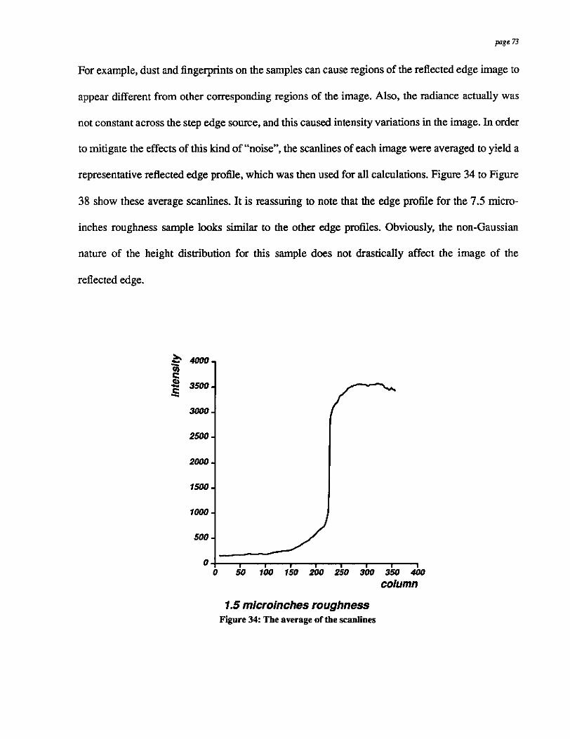
For example, dust and fingerprints on the samples can cause regions of the reflected edge image to
appear different from other corresponding regions of the image. Also, the radiance actually was
not constant across the step edge source, and this caused intensity variations in the image. In order
to mitigate the effects of this kind of “noise”, the scanlines of each image were averaged to yield a
representative reflected edge profile, which was then used for all calculations. Figure 34 to Figure
38 show these average scanlines. It is reassuring to note that the edge profile for the 7.5 micm-
inches roughness sample looks similar to the other edge profiles. Obviously, the non-Gaussian
nature of the height distribution for this sample does not drastically affect the image of the
reflected edge.
1 0 50 loo 150 200 250 3m 350 400
wiumn
1.5 microinches roughness Figure 34: The average of the scanlines
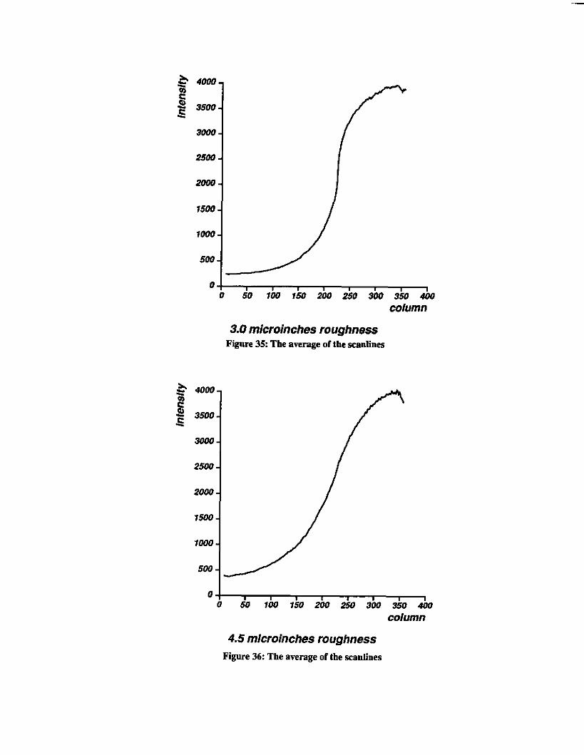
0 50 100 150 200 250 900 550 400 column
3.0 microinches roughness Figure 35: The average of the scanlines
0 50 100 150 200 250 300 950 400 column
4.5 microinches roughness Figure 36: The average of the scanlines

0 50 100 150 200 250 300 3SQ 400 wlumn
7.5 microinches roughness Figure 3’1: The average of the scanlines
- i5 401111- z g 3500- -
m0Q-
2500 -
2000 -
1500 -
1000 - 500 I
0 50 100 150 2w 250 3QQ 350
- i5 401111- z g 3500- -
m0Q-
2500 -
2000 -
1500 -
1000 - 500
9.5 microinches roughness Figure 38: The average of the wanlines
I 0 50 100 150 2w 250 3QQ 350

The algorithm was then run on all five images; the best fit values of the parameters for each
sample are shown in Table 5. Let us list the meanings of the six parameters again for the sake of
clarity,
A - the magnitude of the specular spike component
+ B - the magnitude of the specular lobe component
+ C - the offset of the reflected edge profile
AI3 - the error in the measurement of the viewing and incidence angles
a - the width of the specular spike component
p, - the root-mean-square slope of the surface as determined by our optical roughness
estimation method. It should be equal to the standard deviation of the FADE
In order to make the roughness parameter easier to understand, we will once again express it
in terms of the angles of the normals to facets, rather than as the slopes of facets.The last row of
Table 5 shows these values in units of degrees. The best fit curves and the data for each sample are
shown in Figure 39 through Figure 43. The solid lines represent the fitted c w e , and the dashed
lines show the average scanline plus and minus the standard deviation of the measured intensities
in each column.
The fits to the data curves appear reasonable by eye, and the values of pop, listed in Table 5
seem to indicate that the algorithm can order the surfaces by roughness. Before we accept these
conclusions, and before we further analyze the results of the roughness estimation algorithm, we
must determine if the fits to the data are truly acceptable.
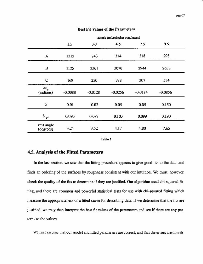
Best Fit Values of the Parameters
sample (microinches roughness)
1.5 3.0 4.5 7.5 9.5
A 1215 743 3 14 318 298
B 1125 2361 3070 2944 2633
C 169 250 378 307 534
A9r (radians) -0.0088 4.0128 -0.0256 -0.01 84 -0.0856
a 0.01 0.02 0.05 0.05 0.150
Po,, 0.080 0.087 0.103 0.099 0.190
rms angle (degrees) 3.24 3.52 4.17 4.00 7.65
Table 5
4.5. Analysis of the Fitted Parameters
In the last section, we saw that the fitting procedure appears to give good fits to the data, and
finds an ordering of the surfaces by roughness consistent with our intuition. We must, however,
check the quality of the fits to determine if they are justified. Our algorithm used chi-squared fit-
ting, and there are common and powerful statistical tests for use with chi-squared fitting which
measure the appropriateness of a fitted curve for describing data. If we determine that the fits are
justified, we may then interpret the best fit values of the parameters and see if there are any pat-
terns to the values.
We first assume that our model and fitted parameten are correct, and that the errors are distrib-

- a 4ooo.00 v1 C $2 s
35m00
30W.00
250~100
2000.00
1500.00
1000.00
500.00 . . . . . . . . - error bars
best fit -
I 0 50 100 150 200 250 300 350 400
column
1.5 microinches roughness
Figure 39: Best fit reflected edge profile and error bars for 1.5 microinches roughness sample

- 0 4500.00
c ti VI
c - 4OW.W
35moo
3m.00
25w.00
2000.00
1500.00
1oIM.00
3.0 microinches roughness Figure 40: Best fit reflected edge pr& and error bars for 3.0 microinches
roughness sample
. . . . . . . . . error bars best f i t -
1 400
column

.- 22 45w.00 z s! .s
4000.00
35W.00
30W.00
2uIo.w
2OOO. w
15w.00
looo.w
500. W . . . . . . . . . error bars
best fit -
4.5 microinches roughness
Figure 41: Best fit reflected edge prome and error bars for 4.5 microinches roughness sample

500. 00
7.5 mlcroiRches roughness
Figure 42: Best fit reflected edge profile and e m bars for 7.5 microinches roughness sample
error bars . . . . . . . . - - best fii
0.00 I

error bars best fit
.- ....... -
I 50 100 150 m 250 900 350 400
column
9.5 microinches roughness
Figure 43: Best fit retlected edge profile and error bars for 9 3 microinches roughness sample

lnge 83
uted normally. x' is a weighted sum of the squared errors, and was defined in equation (37). Let v
represent the number of degrees of M o r n in the problem, thar is, the number of data points
minus the number of parameters. If xL and v are approximately equal, then the fitted curve lies
within the error bars at most points along its length, and the fit is good. We can quantify this idea
with the variable Q , which represents the value of the incomplete gamma function, and gives the
probability that the value of chi squared would be higher purely by chance than the measured
value. Thus, a value of 0.5 shows a good fit, and most researchers accept values greater than or
equal to 0.05 as indicating a good fit. Values much lower than this indicate that our assumptions
are violated, and that either the model or the values of the fitted parameters are probably incorrect.
The statistics quantifying the goodness of the fits are shown in Table 6. Although the predicted
edge profiles are close to the data profiles, the fits are not acceptable.
Chi squared value for the fit
2 e sample x V
180974 54322 0.000000 1.5 microinches
3.0 microinches 18077 1 54322 0.000000
127972 54322 0.000000
161844 54322 0.000000
104902 54322 0.000000
4.5 microinches
7.5 microinches
9.5 microinches
Table 6

It is obvious from the graphs of the fitted curves and the data, Figure 39 to Figure 43, that the
fits, even though they are not technically acceptable, are nonetheless useful, and perhapes even
reasonable. Why, then, do we obtain such low values of Q? There are several possible reasons.
First, the model of the reflected light, equation (18). is technically incorrect. The specular lobe
component of reflection may be described by geometrical optics and a Facet Area Distribution
Function only for very rough surfaces (those for which therms roughness is much greater than the
wavelength of the light).peckmann and Spizzichino 631 In this case, there should be no specular
spike component, and thus, for all our samples which showed an appreciable spike component,
this equation is not appropriate. Notice the general downward trend in the values of x L with
increasing roughness. This is presumably because the model is more applicable to the rougher
surfaces. Another possible cause of error is the non-Gaussian distribution of the heights of the
surfaces. Since the 7.5 microinches roughness sample had the height distribution which differed
the most from a Gaussian, we would expect the error between its fitted and data profiles to be the
highest of all the samples. However, the emrs of the fits decrease monotonically as the values of
and pop, for the surfaces increase. We may thus conclude that although the non-Gaussian p v o f l
nature of the height distribution may contribute to the error, it is probably not the main cause. This
indicates that our algorithm will probably function reasonably for surfaces which do not have a
Gaussian height distribution. A third cause of the error is the fact that the source does not have a
uniform radiance. This was the origin of the large error bars in the data curves; the noise in the
camera is not this great. We could reduce this error by modelling the radiance pattern of the
source; this could be a topic of future research, and would yield some improvement in the quality
of the fits. Note also on the right hand side of all images that the intensity drops off, rather than
levelling out or increasing. This is possibly due to the finite extent of the piece of paper which

acted as the step edge source, but more likely is due to the blurring by the camera of the dark
region beyond the sample into the region of interest. This occurs because the camera is focused on
the edge of the reflected image of the source, rather than on the sample surface itself. Therefore,
some blurring of the edge of the steel disk occurs.
Perhaps the most likely cause of the low values of Q , however, is irregularities of the surfaces
themselves because of contamination and inconsistencies in the milling process. Many of the
short-range variations in the data curves are in fact reproducible, and hence indicate the presence
of contaminants or regions of differing roughness which cause intensity variations much larger
than the noise level. Consider Figure 44. This is a magnified version of the lower left part of Fig-
ure 39, the best fit and measured edge profiles for the 1.5 microinches roughness sample. As we
can see, the variation in the measured curve is much greater than the error in the curve over much
of this region. Other images of this sample, taken with different step edge sources and with differ-
ent viewing angles, show the same pattern of intensity variations. Obviously, these intensity fluc-
........ .... ........ ......... ......... error bars best fit -
140.00 ! I I 1
10 20 30 40 50 60 m 80 90 column
Figure 44: A close-np view of part of tbe best fit curve aid error bars for the 1.5 microinches roughness sample. The measured intensity variations are larger than the error and a p p r in
all images d the sample.

tuations are due to variations of the surface itself, which are, in turn, probably due to
contamination. h order to improve our fits, then, we would have to model the location of surface
defects.
The introduction of additional parameters to describe these sources of error would slow down
the fitting algorithm and possibly affect its convergence. Since our fits capture the shape of the
edge profiles well, we choose to accept them as they are and not modify our algorithm to model
surface defects or any of the other causes of error listed above.
Since we have decided to accept the fits to the data as they are, we will forge ahead,
undaunted, into our analysis of the fitted parameters. The first thing we note is that the values of
the rms slope found by our method are not the same as those found with the profilometer and
listed in Table 3. In fact, the values found by our curve-fitting method do not even fall into the
range of possible values of pprofl as calculated from the profilometric data, although the two sets
of values are of the same order of magnitude. This discrepancy could be due to the poor quality of
the estimates of the correlation length, or to the fact that two different methods of measurement
were used for these calculations. It is also interesting to note that the optical values of the rough-
ness parameter, p,,, are higher than the values found with the profilometer, pprofl. We stated ear-
lier that the opposite behavior is common in roughness measurement systems. Therefore, the
existence of differences between pprofl and pop, was really not unexpected, but the relative mag-
nitudes of the values was surprising. This observation, plus the fact that the values of p,,ofl, and
pop, are so different seems to indicate that the algorithm might not be able to accurately estimate
the rms slopes of the surfaces. The second point of note about the fitted values is that the fitting
process correctly orders the samples by roughness. The values found for pop, are reasonable, and

are similar to those found by other computer vision researchers.[Novak 921 These facts show that
our algorithm might be useful for the accurate measurement of surface roughness. On the basis of
these two conflicting pieces of information, we must therefore conclude that the algorithm can
order the surfaces correctly by roughness, but that its use as part of a mensuration scheme is ques-
tionable.
One of the most interesting things to note about the results of the fitting process is that a, the
width of the specular spike component of reflection, increases with increasing roughness. This is
not predicted by our model, and is a significant finding. It should be included in all future com-
puter vision models of the reflection of light from rough surfaces. It might be possible to exploit
this variation of a with respect to roughness in other roughness estimation systems. The fact that
the specular spike component is so localized might cause problems, however, because the data
will be present in only a small part of the image, but it will also avoid problems associated with
the reflected image of the edge running off the bounds of the image. More research will be neces-
sary to determine the functional dependence of the spike width on the surface roughness.
We next note that the value of C tends to increase with increasing roughness. This is probably
because the image does not contain the entire edge profile for the rougher samples, and the algo-
rithm mistakenly assigns a higher value to C to compensate for the brightness due to the missing
part of the edge. This effect seems to be of minor consequence.
As we have seen, our method of fitting a six-parameter curve to the reflected edge profile does
a good job of matching the appearance of the reflected edge, even though the curves are techni-
cally not acceptable fits to the data. The parameter j3 allows us to order the samples by roughness,
and, surprisingly, the parameter a also increases with increasing roughness, indicating that we
may use this parameter, too, in ordering the surfaces by roughness. Although the method might
not be useful for the accurate measurement of therms slope of a surface, it can differentiate sur-
faces on the basis of therms slope.
4.6. Summary and Discussion
We have shown in this chapter that if we model the reflection of light from our samples with
the theory of Beclanam and Spizzichino, we may obtain reasonable fits to the reflected images of
step edges. We introduced an algorithm which fits a six-parameter function to the profiles, and
orders the surfaces correctly by roughness; the non-Gaussian nature of the surfaces does not seem
to affect this ability. Perhaps the most interesting discovery is that the width of the specular spike
component is a function of the roughness. We have no explanation for this phenomenon, and we
believe that more research will be necessary to determine its cause and its exact functional rela-
tionship. We noted that it might be possible to exploit this relationship in order to measure rough-
ness.
Our roughness estimation algorithm seems to be an acceptable way of quantifying the rough-
ness of surfaces. It is especially useful in situations in which the environment can be controlled,
such as mensuration schemes. However, in a more general purpose vision system, we might not
have such control of the environment, and perhaps we will not have all of the reflected image of
the edge, which, as we noted in the previous chapter, could cause problems in the roughness esti-
mation. Therefore, we intend to look for more robust methods to estimate the roughness; addition-
ally, we will look for more general models of rough surfaces, for use with these new methods.
5. A Direct Roughness Estimation Method
5.1. Chapter Overview
The method of roughness estimation presented in Chapter 4. seems io work fairly well. It can
order surfaces by roughness and provide good fits to the reflected edge profiles, but the veracity of
the calculated rms slope may be questioned There are some other shortcomings of the method
which we will discuss presently. We would like to find a method of roughness estimation which
does not suffer from these difficulties. Therefore, we present a modified form of the reflected radi-
ance equation and discuss its significant features. We will show that it is an example of a type of
thoroughly studied, easily solvable equation. We then present a method of roughness estimation
which uses this equation and calculates a roughness measure directly, thereby avoiding the prob-
lems of local minima in the search space. We first test this method on the images of our samples
from Chapter 4., then use this algorithm on images of our samples for which the iterative method
failed. We show that the new method of roughness estimation obtains results for the situations in
which the previous method did not work. We finally discuss the shortcomings of this method and
directions for future research.
5.2. Shortcomings of the Iterative Method
We saw in the last chapter that we may find the roughness of a reflective surface by fitting a
six parameter function to the image of a reflected edge. In order to do this, we need to know the
position and orientation of the surface, as well as the position of the source and camera. The
method works fairly well but we were unable to determine if it would be useful as a mensuration
tool, since we could not measure the rms slope of the surface by other means. There are some
other problems with this method, also, largely due to its iterative nature. Let us show the situa-

tions in which this methcd fails, and then find the cause of these failures.
Consider Figure 45. Here we see the average profile of a reflected edge for the 1.5 micro-
inches arithmetic roughness sample. The perpendicular distance from the plane of the reflective
surface to the some is 0.322 meters and the viewing angle is 8 degrees. If we run our iterative
algorithm on this image, we find the best fit values of the parameters to be A equal to 1321, B
equal to 712, C equal to 438, equal to 0.042, and a equal to 0.01. Figure 46 shows the best fit
curve and the error bars for each pixel. If we compare this fit to that found for the same sample in
Chapter 4.and shown in Figure 39, it is obvious that the new fit to the reflected edge profile is not
as good as the earlier one, even though the viewing angle is almost the same and the source-object
distance and object-camera distance differ little from the values in the previous experiment. The
value of p is also quite different from that calculated in the last chapter.We took eight other
images with this sample and with different configurations of source, sample, and camera; the
results of the fitting algorithm appear in Table 7. Again, we see that the values are quite different
than those found in the last chapter, and that they vary greatly amongst themselves. They seem to
decrease with increasing viewing angle, er. and with increasing source-object distance. Obvi-
ously,there appears to be a problem with the repeatablility of the method, and with its sensitivity
to the viewing angle and the position of the source relative to the reflective object.

- & 4oM)m- g g 5500.00- -
2500.m - 2ooo.w -
1501200 - 1 m m -
I 204 250 3w 350 400 450 500
z s! 950000- C -. 3ooo.W-
2500.00 - m a 0 -
::!--J, 5m.00 204 250 3w 350 400 , 450 , 500 I
column Figure 4 5 Average reflected edge profile for the
1.5 microinches roughness sample
........ -2 ...... r- ........
am I 204 250 300 350 400 450 500
column Figure 46: Best fit curve and error bars for 1.S
microinches rougbness sample

or (deg) P image source distance (m) camera distance (m)
1 0.322 1.540 8 0.042
2 0.368 1.540 20 0.054
3 1.423 1.540 20 0.017
4 0.320 1.540 45 0.013
5 0.598 1.545 30 0.013
6 0.223 1.545 30 0.036
7 0.071 1.545 30 0.073
8 0.714 1.545 30 0.023
9 1.016 1.545 30 0.024
Table I: The calculated rim slope for the 1 5 microinches roughness sample for several som-object-camera configurations.
There are other problems with the iterative method of roughness estimation. Consider Figure
47, which is the best fit curve and error bars for image number eight. The method used by the
algorithm to find starting values for the fit was described in Chapter 4. If we instead start our algo-
rithm from the best fit values for image number five, i.e. A equal 1277, B equal 723, C equal 525,
p equal 0.013, and a equal 0.00, it will converge to the solution A equal 1165, B equal 837, C
equal 554, p equal 0.007, and a equal 0.00. Figure 48 shows the best fit edge profile and error
bars forthis solution.. The Erst solution has X' = 235922 and the second has x* = 128496, show-
ing that the second is a better fit. Thus, we see that there exist local minima in our search space,
and that we may get different estimates of the roughness, depending on the starting guesses in our

......... error bars bestfit -
- 5 4ooo.00- I2 s? e 35oa00- c
3 m 0 0 -
25OO.00 - 2004.00 -
7500.00 - fwo.00 -
500.00 I
column 150 m 250 300 3511 400
Figure 47: Best fit edge pmtile and error bars for image number eight. This fit used the default starting values in the mnghness
estimation algorithm.
c.. /u----+ ......... .......
..a .f
......... error bars best fa -
500.00, I I I 1
150 2w 250 300 350 400 column
edge pmtile and error bars for imaEe number Figure 48: Best eight. This fit used the best fit parameters for image number five as
its starting values.

algorithm
9m.w - 2500.00 -
2m.w - 15W.W -
lw(1.W-
The cause of these problems is not hard to discover. As we discussed in Section 3.3., unless
we have the full reflected edge profiles, it is hard to differentiate some profiles which belong to
surfaces with different roughnesses. In fact, almost all edge profiles, regardless of roughness, will
appear the same if we consider a small enough portion of the edge profile, so that any differences
behveen the curves is less than the noise in the images. Figure 19 shows this clearly. In Figure 49,
we plot a shifted version of the average edge profile for image number 5 and the error bars for
image number 8. We see that the average edge profile lies between the error bars for most of its
extent, and therefore, images number 5 and 8 are essentially indistinguishable. Since the geornet-
r i d configurations which formed these images were quite different, the fitted parameters differ,
even though the images are quite similar. This explains the widely varying values found in the
most recent series of experiments. The indistinguishability of the profiles also contributes to the
error bars . . . . . . . . . I - average
1 900 350 400
Figure 49: The average edge pro6le for image number five, and the error bars for image number eight The average profile lies witbin
the error bars for most of its extent
5w.w , 150 200 250
column

Plgc 95
problems with local minima. The existence of local minima is determined by the form of the fitted
equations, but the indistinguishability of profiles makes it more difficult to find the correct starting
values, and easier to fall into a minimum, since there is less curve to differentiate solutions. Con-
versely, if we have the full reflected edge profile, we should be more likely to find the p r o p
roughness value for a surface. Image number 7 bears out this hypothesis. The source to object dis-
tance for the experiments of Chapter 4. was 0.096 meters and the viewing angle was 7.29 degrees.
The distance for image number 7 is 0.W1 meters, meaning that we probably have most of the
reflected edge profile in this image, even though the viewing angle is 30 degrees. The fitted value
of is 0.073, which is the largest of any values found in this series of experiments, and which is
fairly close to the value found in Chapter 4., which was 0.080. Therefore, we believe that the iter-
ative method worked correctly on this image.
We may rightly ask if our results from the last chapter may be trusted. There were five san-
ples in the experiments of Chapter 4., with arithmetic average roughnesses of 1.5, 3.0, 4.5, 7.5,
and 9.5 microinches. As we stated above, unless we have the full edge profiles, our results are
questionable. The images for the fist four samples contained large portions of the profiles, and
this indicates that we may trust the calculated values. The image for the 9.5 tniminches sample
did not show the full edge profile, but the surface roughness was ordered properly. Therefore, we
feel that the value for this sample may not be exactly correct, but is probably close to the correct
value. Additionally, we used our iterative algorithm on these images, but used different starting
values, and found that it converged to the same results. Thus, we believe that we can trust our
results from the last chapter.
Our most recent series of experiments has shown that there are some shortcomings to the iter-

pate 96
ative method of roughness estimation. We can only conclude that in order for the method to work,
we must have most of the reflected edge profile, but that if we do have this, the method works
well. Let us now look for a method which does not require the full edge profile, and which will
not become trapped in local minima of the search space.
5.3. Reflected Radiance Equation
5.3.1. Modified Reflected Radiance Equation
We now wish to devise a method of roughness estimation which does not have the problems
of our iterative method. In order to do this, we will modify the reflected radiance equation
slightly, so that we may use alternative methods of solution.
Let us return to the equation for the reflected radiance due to an extended source, equation
(23). Once again, this is
where ef is the facet n o d angle, 0, is the viewing angle, S(O$ is the FADF, a quantifies the
spread of the specular spike, A and E are constants relating the strength of the spike and lobe
components, and I gives the radiance of the source. We have taken the liberty of replacing the first
term in the integrand by its approximation, which we derived in Chapter 3.. As we noted in that
chapter, A and B can take on any values and can thus represent any source intensity. Therefore,
we will absorb l into the definitions of A and B and I will no longer appear in the equation. Now,
let us consider the limits of integration. As we showed in Chapter 3.. for every point on the sur-
face, there will be a range of values of e, for which light will be incident on the surface from the

m e 97
source and will then reflect into the camera. This range will change from point to point on the SUT-
face. We may phrase this another way if we change OUT focus of attention from the source-object-
camera configuration to the reflective object itself.
Consider a generic FADE The value of the FADF for an infinitesimal range of values of Of is,
by definition, the ratio of the area of facets with their normals in this range to the area of the mean
surface. For essentially all surfaces, the FADF will be bounded, that is, there will be two values of
Of, beyond which the FADF equals zero. Obviously, the values of ef will always lie between -: and 5 , since a higher value would imply that the surface has “folded over” on itself, and we study
only single-valued surfaces. For most surfaces, however, the range of facet angles will be much
smaller than this. Let us call the endpoints of this range efmimi. and efmx. If the range of integration
does not overlap the range of non-zero values of the FADF, there will be no light reflected. If the
range of integration overlaps the range of non-zero values of the FADF, there will be some facets
on the surface which will reflect light from the source to the camera. Figure 50 shows several
schematics of a some, object, and camera. The schematics show the range of all facet orienta-
tions, the directions of some incident light rays, and the direction of the reflected ray for different
points on the surface. In all the diagrams, the angles of the facet n o d s which actually do reflect
light from the source to camera are Wed in with black. In this series of diagrams, the range of fac-
ets which reflect light varies, but, so long as light is reflected, this range always contains the end-
point closest to the source. Therefore. in equation (39), the final value of the range of integration
varies as a function of the position on the surface, but the initial value remains the same. For the
region of the surface for which one of the endpoints of the range of integration stays fixed, we
may write equation (39) as

source
/
No light retlected
1 Some facets reflect light into the camera
%
More facets reflect light into the camera
I AU facets reflect light into the camera
Figure 50: Different groups of facets will reflect light from the 80m into the camera for dflerent points on the surface. The directions shorn in black are the normals to t h w facets which reflect light from some
point on the source into the camera.

As before, e, is a function of xobj. Naturally, we will obtain the same form for the equation if
remains constant rather than e,min. If we know the relative positions of the source, reflective
surface, and camera, it is not difficult to calculate which points are in the region for which the
starting value of the range of integration is fixed.
Of=
Let us now modify the equation slightly in another way. Consider the ratio
The reason for studying this function will become apparent shortly. Let US multiply the fist term
in the integral by this ratio; the FADF in the second term is already multiplied by it. As long as
the ratio remains close to one, the approximation will be justified. It is easy to see that the ratio
approximates unity for small values of er. Now, the values of a remain fairly small; in fact, for
our roughest sample, the 9.5 microinches sample, the value of a was found to be only 0.150. This
implies that the value of the exponential in the fist term of the integral will be appreciable only
for small values of 0,. and thus, the ratio will contribute to the integral only when its value is
approximately equal to one. For example, for e, = 0.150, a = 0.150, and 0, = 45 degrees, the
exponent will equal e-', and the ratio will be equal to approximately 1.138. Its value will be even
smaller for most of our imaging situations. Therefore, for all values of e,, for which the exponent
is appreciably larger than zero, our introduction of the ratio will change the value of the integral
only slightly. With this change to equation (40), we may factor the integrand, and the equation for

the reflected radiance becomes
Let us multiply both sides of the equation by cme, to make the important things about this
equation more clear. We then obtain
There are several interesting things about the form of this equation. Fist of all, note that it is
very similar to a convolution. The only difference between this equation and a convolution is that
the limits of integration of a convolution would be -E and x , rather than h i t e values which vary
from point to point on the surface. Therefore, it might be possible to use Fourier methods to solve
for the quantity
Additionally, it is possible to make a different approximation and cast the reflected radiance
equation into true convolution form; details appear in Appendix 2.
Next, note that this is also an integral equation. A general integral equation is of the form
where U(X) is the unknown function, and f ix) and K(x, t) are known. If h equals zero, this is called

page IO1
afirsr-kind integral equation. If the upper limit of integration, b , is equal to x or a function of x , it
is called a Volterra integral equntion. Therefore, equation (42) is a first kind Voltma integral
equation. Unlike many other first kind integral equations, first kind Voltena equations are usually
stable with respect to inversion. Just as with the convolution, we may use the methods of solution
for Volterra equations to find
This is the weighted sum of the FADF and a Gaussian. We will use this function to quantify the
roughness of surfaces.
Therefore, by modifying the reflected radiance equation slightly, we put it into a form which
can be solved in two different ways. The function for which we will solve is a weighted sum of
the FADF and a Gaussian, and we must discover how we may use this to estimate roughness.
5.3.2. Solution of the Modified Reflected Radiance Equation
We showed in the last section that if we make some small changes to our description of the
reflection of light from rough surfaces and the reflected radiance equation, the form of the
reflected radiance distribution is governed by an equation which is similar to a convolution and is
also a first kind Volterra equation. We must decide whether we want to solve the equation with the
methds applicable to convolutions or those for use with Volterra equations.
We have decided to attack the problem of solving equation (42) with the methods suitable for
Volterra equations. We feel that these methods are simple, and yield good results. In this section,
we develop numerical, rather than analytical, methcds of solution.

p g e 102
In order to solve the equation, fist consider a point on the surface. Because 15~ and e7 are
known at every point, we may calculate L,cosB,, which is given by
<Y where u(e9 = Ae
mate the integral by the sum
+BS(B>. We may then discretize the variable of integration, and approxi-
We must decide on the number of function evaluations, N, which will be used in the sum, and the
size of the steps, Aefi. Figure 50 will help us with this endeavor. Let us start at a point on the sur-
face where the reflected edge profile is dim, and move perpendicular to the reflected edge, in the
direction of increasing brightness. For most singly-curved surfaces, a larger pomon of the facets
will reflect light into the camera as we move from point to point on the surface in this direction.
The change in the endpoint of the range of facets will be the obvious choice for Aefi. For every
point in the edge profile, then, the number of function evaluations wiU be the same as the position
of the point in the profile. For example, for the first point in the profile, there will be one term in
the sum, for the second, two terms, for the third, three terms, and so on. Therefore, if we let i
denote the position of the measured radiance along the edge profile, we will obtain a matrix equa-
tion of the form
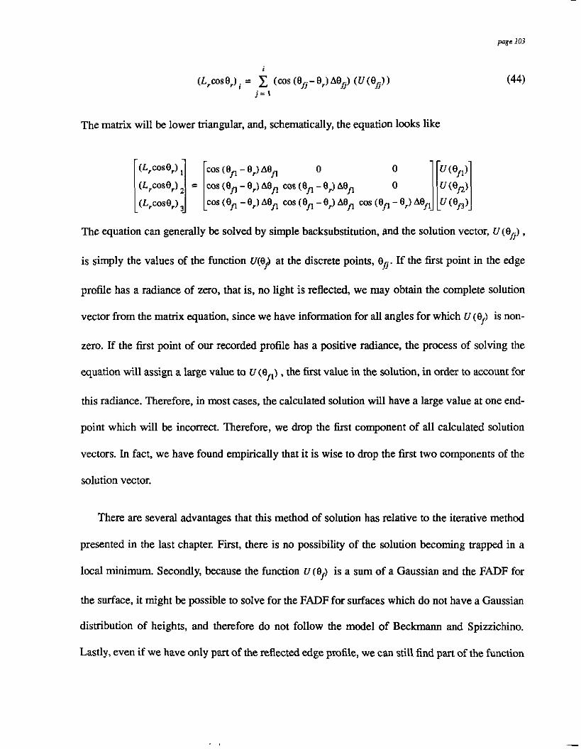
The matrix will be lower triangular, and, schematically, the equation looks like
(L,wse,) I cos (e - er)Ae,, 0 0
(L,wser) = (eP P - er) Ae,, COS (e, - e,) &efl 0 ]pj 1 cos(eP-e,)Aef l wsce,-ejAe, m(efl-er)Aefl u(e,)
The equation can generally be solved by simple backsubstitution, and the solution vector, (I (0,) ,
is simply the values of the function u(e+ at the discrete points, efi. If the first point in the edge
profile has a radiance of zero, that is, no light is reflected, we may obtain the complete solution
vector from the matrix equation, since we have information for all angles for which (Icef) is non-
zero. If the first point of our recorded profile has a positive radiance, the process of solving the
equation will assign a large value to (I (e,) , the first value in the solution, in order to account for
this radiance. Therefore, in most cases, the calculated solution will have a large value at one end-
point which will be incorrect. Therefore, we drop the first component of all calculated solution
vectors. In fact, we have found empirically that it is wise to drop the first two components of the
solution vector.
There are several advantages that this method of solution has relative to the iterative method
presented in the last chapter. First, there is no possibility of the solution becoming trapped in a
local minimum. Secondly, because the function U (Of) is a sum of a Gaussian and the FADF for
the surface, it might be possible to solve for the FADF for surfaces which do not have a Gaussian
dismbution of heights, and therefore do not follow the model of Beckmann and Spizzichino.
Lastly, even if we have only part of the reflected edge profile, we can still find part of the function

p g e 104
U(ef) . Of course, we must determine if the corruption of the data by noise will prevent the
achievement of these goals.
The first-kind Volterra integral equation form of the reflected radiance equation provides a
new way of describing the reflection of light from rough surfaces, and new methods of solution
for the FADF. We must now see how we can use the results of this equation to quantify surface
roughness.
5.4. Width Measures
Although we may use the new method of solution to find the FADF for any surface for which
we have geometrical reflection, it is probably unwise to take the resulting function too literally,
since noise may corrupt the shape of the calculated function. Perhaps, however, there exist other
quantities which we may derive from U($) in order to estimate the surface roughness.
5.4.1. The Variance
In earlier chapters of this thesis, we repeatedly referred to the “width” of the Facet Area Dis-
tribution Function, denoted p, and stated that it represented the roughness of the surface. This
quantity is related to the standard deviation of the distribution function. Perhaps we can find a
similar quantity for the function u (ef).
Although we have not yet assumed a specific model of the FADF in the calculations of this
chapter, in order to continue with ourcalculations, we must now do so. As in other sections of this
thesis, we assume the model of Beckmann and Spizzichino. Therefore, we substitute this FADF
into the function u(ef), to obtain

p g c 105
(45)
Let us now calculate the “width” of CI ( ef)
Perhaps the most common way of quantifying the width of a probability density function is to
find its variance or its standard deviation, which is the square root of the variance. If F ( x ) is a
probability density function, normalized so that
the mean value of the distribution is
and the variance of the distribution is defined to be
Let us perform these calculations for the function u(ef) . We will not perfom a strict normaliza-
tion or calculation of the variance, but rather related calculations.
We must first normalize the function; therefore, we must find the value of its integral so that
we may divide by this number to normalize u(e,) . The calculations are actually easier if, rather
than finding the value of the integral, we find a related quantity which we denote N. We thus form

page I06
As we commented in Section 53.1.. a is a small number, and therefore, the first term of the inte-
gral will contribute to N only for small values of Or Therefore, we will approximate case, by 1 in
the 6rst term of equation (47). For e, equal to 0.150, which we found for a for our roughest sam-
ple, cose, is approximately 0.989, and it differs from 1 by only 1.1 per cent; our approximation is
thus reasonable. With this change, equation (47) becomes
z 2
We solve equation (48) to find
N = A & a + B (49)
Because u(e,) is symmehic about zero, its mean value is zero. We may now find a quantity akin
to the variance by forming
This time, we approximate ~ s e f ( t a d f ) ' by 0; in the first term of the integral. For 0, equal to
0.150, the difference is only about 0.38 percent of the c o m t value. We then find
3 2 A h a + B p 2 ( A h a + B )
var =
We would now like to determine if this is a useful quantity for characterizing roughness. We

page 107
mean “roughness” in the intuitive sense, rather than actually choosing nns heights or rms slopes
as our roughness parameter. Although we do not know the exact dependence of the four parame-
ters, A , B , a , and p on the roughness, our experiments have given us some rules of thumb. As the
surface roughness increases, a and p increase. In fact, we could choose these parameters to be our
definition of roughness if we so desired. B tends to increase or remain constant with increasing
roughness, while A decreases with increasing roughness. How, then, does this variance-like quan-
tity change with increasing roughness? We let p represent this intuitive roughness and calculate
We know that
and
The parameters must be larger than zero, and p is always larger than a . Therefore,

page io8
a(var)>O aB
ab
and can take on both positive and negative values. Our "rules of thumb" state that
g<0
E,O
dP
dP
@ > O dP
and
Thus, the derivative of this quantity with respect to roughness can take on both positive and nega-
tive values. As a result, there exist local minima in the space of its possible values. Numerical
experiments conlirm this. Since this variance-like quantity does not vary monotonically with
respect to roughness, it is not a suitable parameter to quantify roughness.
We must now look for a function which, like the variance, measures the width of the dishibu-
tion, but which varies monotonically with respect to the roughness.
5.4.2. Our Width Measure
In the last section, we studied a width measure that was related to the traditional measure of

the width of a distribution, the variance. We showed, however, that it is unsuitable for estimating
the roughness. We must now look for a related, but more useful, function. In this section, we will
introduce a new function which we have developed that serves this purpose.
Consider once again the function,
At e, = 0, the function takes on its maximum value, A +
constant, rather than N. This means that we make the maximum value of the distribution equal to
one. Now, the function we want to study is
Let us use this as our normalization J i b '
For lack of a good name, let us simply refer to this new function as our width measure, W. It is
equal to
We again let p represent the intuitive roughness and calculate
,

p g e 110
We know that
and
The "rules of thumb" are the same as they were in Section 5.4.1., and therefore, W increases with
increasing roughness for all physically realizable values of the parameters. Thus, our width mea-
sure, and the Volterra equation description of the reflected step edge which allows us to calculate
it, provide a new method of roughness estimation. Let us perform experiments to determine the
usefulness of this method.
5.43. The Effects of Noise
As in any experiment, OUT results will be cormpted by noise. Therefore, we must study how
noise will affect our calculations, and then devise methods to correct for this. We obtain many
reflected edge profiles in OUT analysis of the image, and we may average these to reduce the
effects of the noise. The question is, should we average the profiles before we perform our calcu-
lations, or should we average the results of our calculations? In the solution of the Voltena equa-

tion, noise will corrupt the calculation of ~ ( e $ . The matrix form of the equation is linear, so that
we will obtain the same answer regardless of whether we average the data before solving the
equation, or if we solve the equation for each profile and then average the results. The calculation
of W , however, is nonlinear, and tends to magnify the effects of noise since we square the term
tanor Therefore, we should average the scanlines before we perform our calculations in order to
minimize the noise going into the calculation of W.
5.5. Experiment
In the previous section, we stated that we wished to quantify the width of the function, UV+) ,
and showed the problems with using the variance, a common width measure. We then derived a
function, which we simply call our width measure and denote by W , which we may use as a crite-
rion for roughness estimation, since it varies monotonically with respect to roughness for a sur-
face with a Gaussian distribution of heights. Let us now calculate W for the images of step edges
reflected in some real surfaces.
5.5.1. Experimental Configuration
In our experiments, we will use the same rough surfaces as we did in Chapter 4. In fact, we
will use the same experimental configuration and images as we did in that chapter, although we
will also perform additional experiments. In Section 5.2., we mentioned these additional images
briefly, when we showed that the iterative method of roughness estimation would not work on
them. We will discuss them again in greater detail now. Let us describe the experimental configu-
ration one more time. Figure 5 1 and Figure 52 show the experimental configuration and label the
important physical quantities.. The source is a large sheet of white paper, illuminated by a halo-
gen lamp, and is parallel to the face of the reflective surface. The distance from the wurce to the

--
page JJZ
top view
halogen lamp
front left view
camera Figure 51: Schematic of the experimental configuration
n . obi Figure 52: The reflection geomehy for the experimental configuration
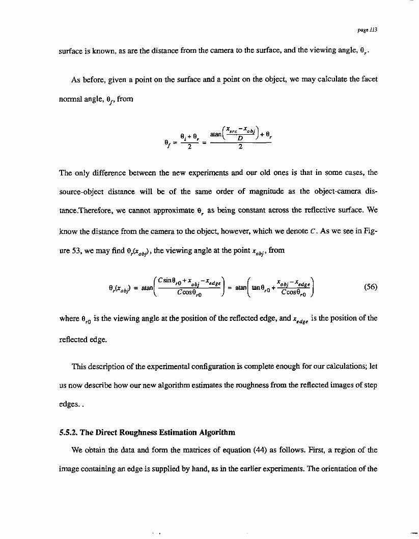
pap 113
surface is known, as are the distance from the camera to the surface, and the viewing angle, e?.
As before, given a point on the surface and a point on the object, we may calculate the facet
normal angle, ef, from
The only difference between the new experiments and our old ones is that in some cases, the
source-object distance will be of the same order of magnitude as the object-camera dis-
tance.Therefore, we cannot approximate as being constant across the reflective surface. We
h o w the distance from the camera to the object, however, which we denote C. As we see in Fig-
ure 53, we may find er(xOb>, the viewing angle at the point xobj, from
where ero is the viewing angle at the position of the reflected edge, and
reflected edge.
is the position of the
This description of the experimental configuration is complete enough for ow calculations; let
us now describe how our new algorithm estimates the roughness from the reflected images of step
edges..
5.5.2. The Direct Roughness Estimation Algorithm
We obtain the data and form the matrices of equation (44) as follows. First, a region of the
image containing an edge is supplied by hand, as in the earlier experiments. The orientation of the

page 114
camera
t
Figure 53: Geometry for the eakulatiw of the viewing angle as a function of position.
edge is also given. Next, the image is scanned perpendicular to the edge to obtain reflected edge
proflees, and the profiles are averaged to yield a representative protile.
The algorithm then starts at the side of the average edge profile with the lower intensity, and,
as per equation (43), records L,(xl)me,(xl), where xI is the position of the point under study. It
next calculates the angle, eed8el, at which a facet would need to be oriented in order for light to
reflect from the edge of the source, off this point of the surface, and into the camera. All light seen
at this point is thus reflected from facets which lie between -E and erddLl. It then finds the mid-
point of this range, denoted Omid l . The [1,1] element in the matrix.is then cos ( €Imidl -8 , )A9, ,
where ABI = eedgeI-(-:)
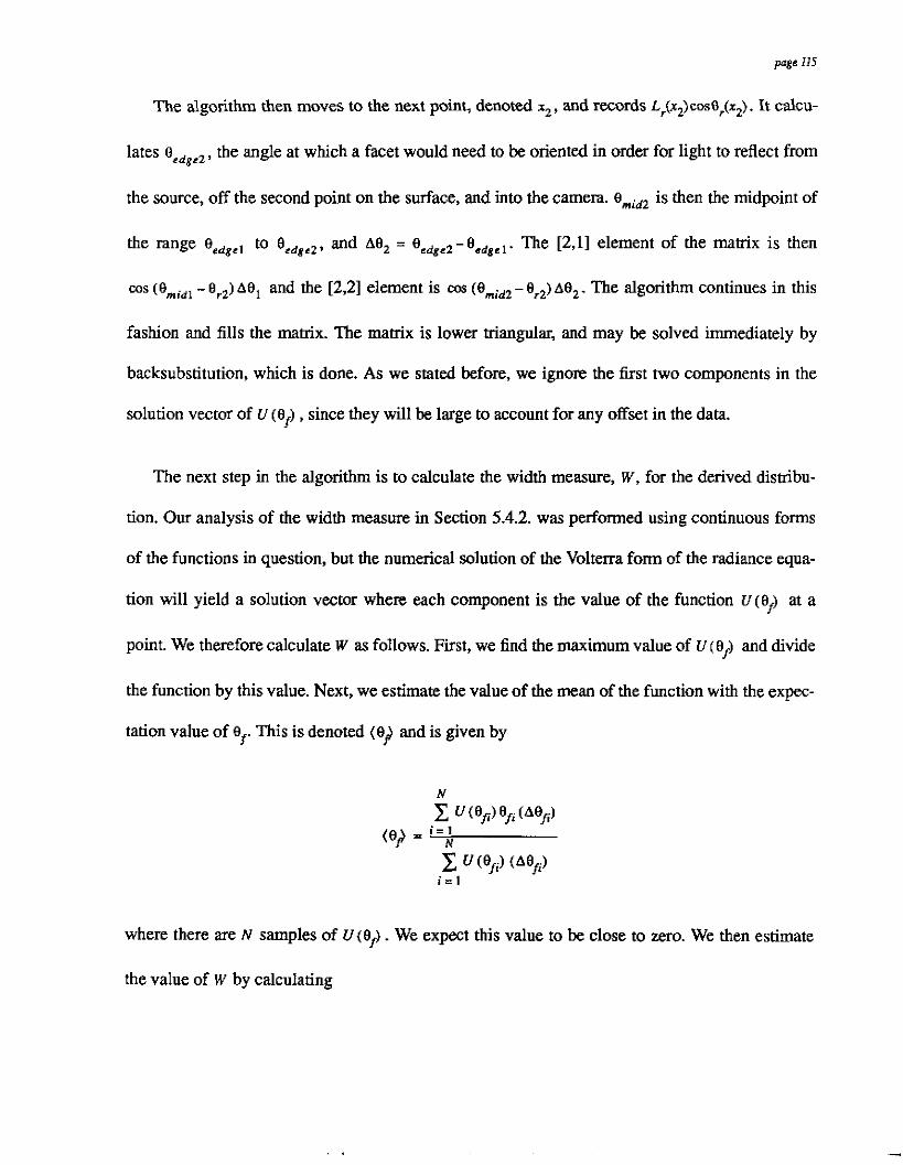
page I15
The algorithm then moves to the next point, denoted x2, and records L,(.x2)cos8,(x2). It calcu-
lates ecdgc2, the angle at which a facet would need to be oriented in order for light to reflect from
the source, off the second point on the surface, and into the camera. BmidZ is then the midpoint of
the range to O c d g r 2 , and Ae2 = eadgc2- e e d g r l . The [2,1] element of the matrix is then
cos (enidl -e,) A e l and the [2,2] element is cos (e , id2-e,2)Ae2. The algorithm continues in this
fashion and fills the matrix. The matrix is lower triangular, and may be solved immediately by
backsubstitution, which is done. As we stated before, we ignore the first two components in the
solution vector of U (ef) , since they will be large to account for any offset in the data.
The next step in the algorithm is to calculate the width measure, W , for the derived dismbu-
tion. Our analysis of the width measure in Section 5.4.2. was performed using continuous forms
of the functions in question, but the numerical solution of the Volterra form of the radiance equa-
tion will yield a solution vector where each component is the value of the function u(ef) at a
point. We therefore calculate W as follows. First, we find the maximum value of U ( ef) and divide
the function by this value. Next, we estimate the value of the mean of the function with the expec-
tation value of Or This is denoted (e$ and is given by
where there are N samples of U t e f ) . We expect this value to be close to zero. We then estimate
the value of w by calculating

page 116
For the smoother of our samples, the results of this calculation are often at the level of
machine precision for our computer. This indicates that most of the terms in the sum of equation
(57) are smaller than the machine precision, and that the calculation suffers severely from the
results of roundoff error. In order to solve this problem, we multiply each term in the the sum by a
constant, which we choose to be loo00. There is no special significance to this number, other than
that the calculated values of the pseudovariance for our samples are generally in the range from 0
to loo.
5.5.3. Old Data
Let us now use our algorithm on the images from Chapter 4., and calculate the width measure
for each. Pictures of these images and the average scanlines for the regions of interest appear in
that chapter. Figure 54 to Figure 58 show u(ef) for each image. The values of the w for each
sample appear in Table 8. As before, the samples are ordered correctly. The differences between
the values of W seem significant, and this would make the mthd useful for roughness differenti-
ation. We must perform more experiments to determine the uncertainty in these calculations, to
see if the differentiation is valid.
5.5.4. New Images
We have seen that the width measure W can order the surfaces by roughness. In order to deter-
mine the usefulness of the method, however, we must determine the uncertainty in these calcula-
tions and see if the method can work for different confignations of some, reflective surface, and
camera. Our next se.t of experiments uses only the 1.5 microinches roughness sample. The experi-

page 117
I -0.25 4-20 4.15 4.10 4.05
-?wow - radians Figure 54: The function V@,) for the 1.5
microinches roughness sample.
I 1 radians dMM0
Figure 55: The function U(O> for the 3.0 microinches roughness sample.

page 118
5
Figure 56: The function U@,J for the 4.5 microinches rnughness sample.
40000 -I Figure 57: The function U(B$ for the 7.5
microinches roughness sample.

I
Figure 58: The function U(e> for the 9.5 microinches roughness sample.
sample (microinches roughness) W
1.5 0.0983
3.0 3.29
4.5 25.5
7.5 16.1
9.5 31.9
Table 8: The value of W for tbe five samples. The images nsed are the same as those in Chapter 3.
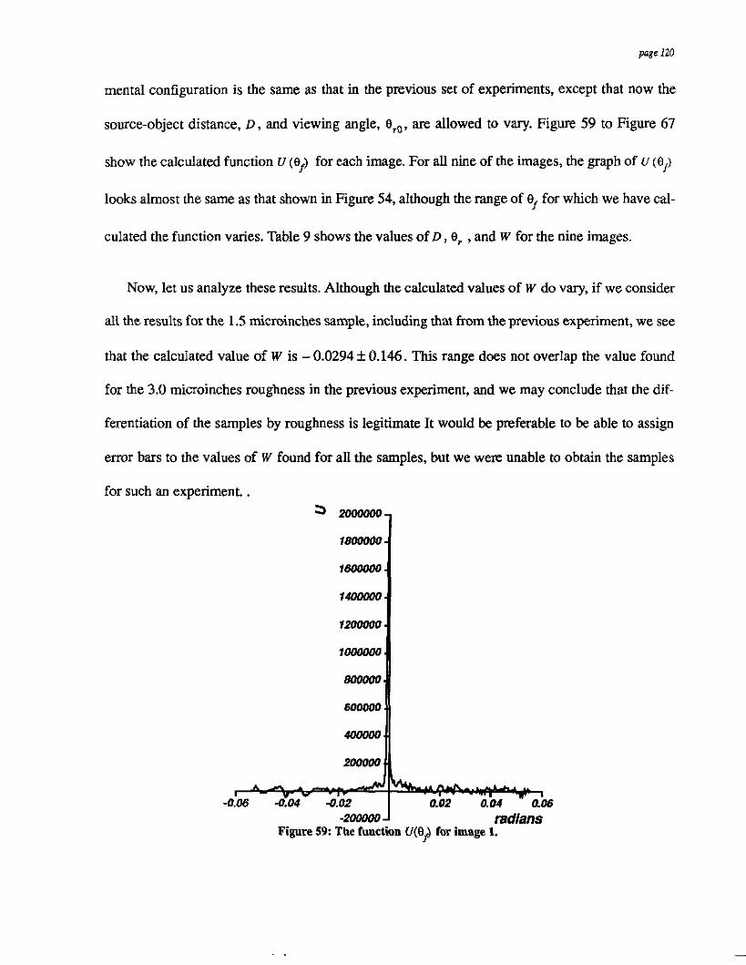
page 120
mental configuration is the same as that in the previous set of experiments, except that now the
source-object distance, D , and viewing angle, gro, are allowed to vary. Figure 59 to Figure 67
show the calculated function U (0,) for each image. For all nine of the images, the graph of u (Of)
looks almost the same as that shown in Figure 54, although the range of e, for which we have cal-
culated the function varies. Table 9 shows the values of D , Or , and w for the nine images.
Now, let us analyze these results. Although the calculated values of W do vary, if we consider
all the results for the 1.5 microinches sample, including that from the previous experiment, we see
that the calculated value of W is - 0.0294 k 0.146. This range does not overlap the value found
for the 3.0 microinches roughness in the previous experiment, and we may conclude that the dif-
ferentiation of the samples by roughness is legitimate It would be preferable to be able to assign
e m bars to the values of W found for all the samples, but we were unable to obtain the samples
for such an experiment. .
-0
Figure 59: The function U(9> for image 1.
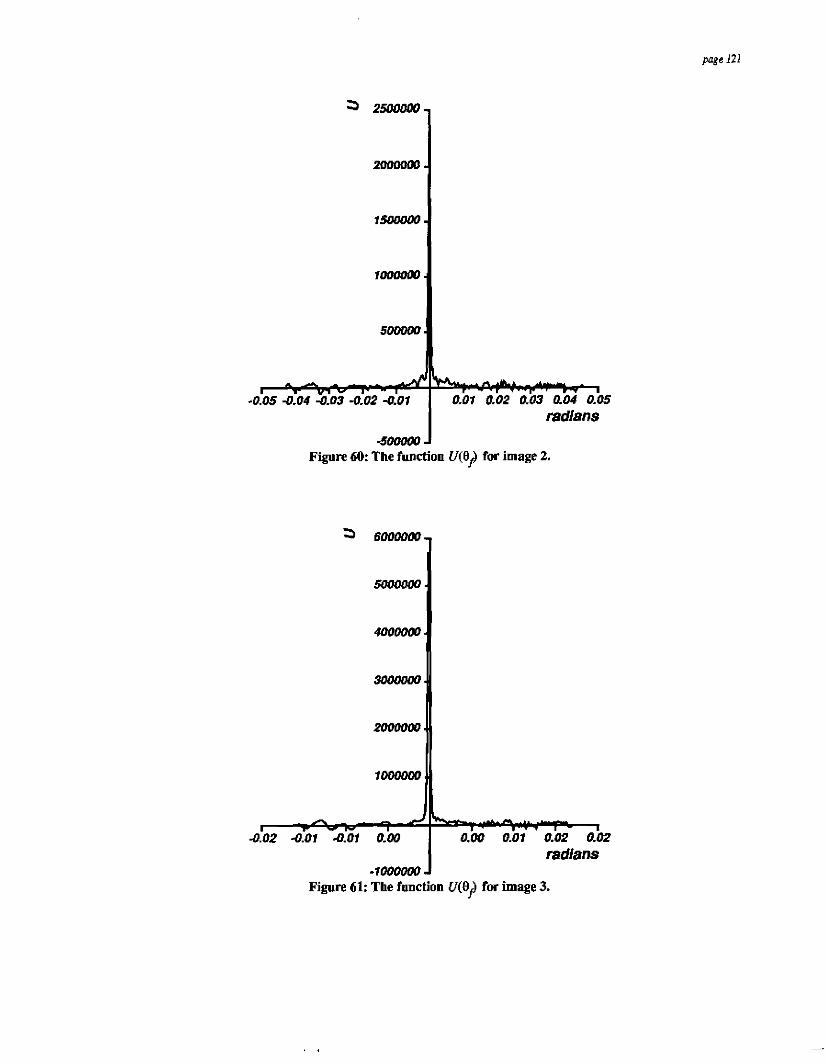
page 121
mmam
QM)(Mw.
Figure 60: The function U(O$ for image 2.
3 SMMOW-,
SOOWW.
2M)IMoo.
looowD

p g e 122
-1owwO Figure 62: The function U(9> for image 4.
radims
3 45ooom
4owow
35ooolm
3LMaaw
25woW
2wwao
15(Mow
lowoW
5WOW - -0.03 4.02 -0.01
-5wMM Figure 63: The function U(9> for image 5.
radians
,

3 1t?oooo6
7600006
14000011
12wooO
lMMMM
800000
6oooW
4MIow)
2 m
w -0.06 4.04 4.02
-2wwoo Figure 64: The function U(fJ'Cer, for image 6.
-1owW radlans
radlans
Figure 6 5 The function U@,J for image 7.

pap 124
3 4 s m
# O m
3500000
SOOOOW
25wMM
2-
1500000
1OMMw
5omm + -0.03 0.02 0.oi 4.01 0.00
radlans s m Figure 66: The function U(O> for image 8.
- mdians
0.00 0.01 0.02 a02
Figure 67: The function U(0J for image 9.
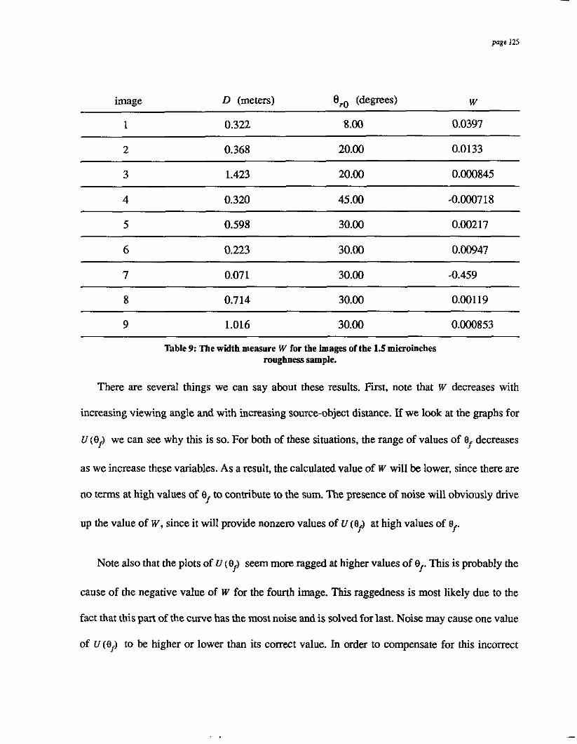
pnge 125
image D (meters) oro ( d e w 4 W
1 0.322 8 .OO 0.0397
2 0.368 20.00 0.0133
3 1.423 20.00 0.000845
4 0.320 45.00 -0.0007 18
5 0.598 30.00 0.00217
6 0.223 30.00 0.00947
7 0.07 1 30.00 -0.459
8 0.714 30.00 0.001 19
9 1.016 30.00 0.000853
Table 9 The width measure W for the images of the 1.5 microinches roughness sample.
There are several thiigs we can say about these results. First, note that w decreases with
increasing viewing angle and with increasing source-object distance. If we look at the graphs for
U (ej) we can see why this is so. For both of these situations, the range of values of et decreases
as we increase these variables. As a result, the calculated value of W will be lower, since there are
no terms at high values of to contribute to the sum. The presence of noise will obviously drive
up the value of W , since it will provide nonzero values of U ( e j ) at high values of er
Note also that the plots of U (ej) seem more ragged at higher values of er This is probably the
cause of the negative value of W for the fourth image. This raggedness is most likely due to the
fact that this part of the curve has the most noise and is solved for last. Noise may cause one value
of U (ef) to be higher or lower than its correct value. In order to compensate for this incorrect
page I26
value, the next point solved for will either lower or higher than its correct value. This may cause
oscillations that build up over time. There are possible ways to solve this problem and improve
the method. For example, we may solve for the function u(ef) twice by starting from both posi-
tive and negative values of ef and then averaging these results. We may also smooth the average
reflected edge profile prior to solution for U (Of). We leave the pursuit of such methods to other
researchers.
Perhaps the most imponant thing that can be said about the second set of experiments is that
results were obtained, and they were fairly consistent and close to that found in the first series of
experiments. This cannot be said of the iterative method of roughness estimation. Remember,
these images did not have complete edge profiles, and the roughness values found by the iterative
method varied widely. Although the results found by this method are not as precise nor as easily
understood as those of the iterative method, the calculation of our width measure seems to be a
more robust method of ordering surfaces by roughness.
5.6. Conclusions
In this chapter, we have shown that although the iterative method of roughness estimation pro-
duces accurate values, it requires most of the reflected edge profile in order to work correctly. In
order to produce a new method which does not require the full edge, we modified the reflected
radiance equation slightly and cast it in the form of a first kind Volterra integral equation. We
showed how to solve the equation numerically and introduced a derived quantity, W , which
increases monotonically with increasing roughness. We calculated W for the images of Chapter
4., and showed that it orders the surfaces correctly. We next calculated W for the images for which
the iterative method would not work. The new method worked, and yielded values close to that

prge I27
found for the image of the 1.5 microinches roughness sample from Chapter 4.
Although it is dimcult to relate physical values such as the root-mean-square height or Toot-
mean-square slope of the surface to this new width measure, the function W does seem to be a
possibly useful function for the differentiation of surface roughness, and should be explored fur-
ther. Perhaps the accuracy of the solution for U (ef) could be increased to allow calculation of the
full FADF of the surface. This would allow us to gain more information about surfaces which do
not follow the Beckmann and Spizzichino model of reflection.

6. Summary and Conclusions
6.1. Summary
In this thesis we have shown that it is possible to estimate the roughness of a surface by study-
ing a single image of step edges reflected in the surface. We derived an equation describing the
appearance of a reflected edge, and have shown that in order to determine the roughness, we must
have knowledge of the relative positions of the light source, the reflective object, and the camera.
Two techniques for estimating the roughness of the surface were presented. The first technique fits
a curve described by the model of the reflected edge to an image of a reflected edge and finds the
root-mean-square slope of the surface. This algorithm could be useful for accurate measurement
of surface roughness. The second technique analyzes the reflected edge profile and calculates a
quantity which we have derived that increases monotonically for increasing roughness and thus
allows us to order surfaces by roughness. This is a more robust method, since it requires less of
the reflected edge image than does the fmt method, and would be more useful for general purpose
vision systems.
6.2. Contributions
There are several contributions this thesis makes to ow understanding of the appearance of
rough reflective surfaces.
This thesis presents a model of the appearance of reflected step edges.
Although many researchers within and without the computer vision field have studied
the reflection of light f?om rough surfaces, they have usually focused on situations with

p g e I29
point light sources. This thesis addresses the effect of roughness on the reflected images
of step edges, since edges are an important low-level visual feature and are used in many
physics-based vision algorithms. It describes how the reflected images of edges change
with respect to roughness.
This thesis identifies the information necessary to determine the roughness of a surface
from a single image containing reflected edges.
In this thesis, we have shown that many different configurations of source, reflective
surface, camera, and roughness can produce images which are indistinguishable to
within noise levels of the camera Therefore, we conclude that in order to calculate the
roughness of a surface from a single image of a reflected step edge, we must know the
relative positions of the source, object, and camera This knowledge is incorporated in
all our methods of roughness estimation.
The experiments discussed in this thesis indicate that the width of the specular spike
component of reflection increases with increasing roughness.
The change in the width of the specular spike component of reflection with respect to
roughness is not predicted by Beckmann and Spizzichino’s theory of the reflection of
light from rough surfaces. Knowledge of this effect allowed us to e u c e a realistic
model of the profile of a reflected step edge.
* The most important contribution of this thesis is the presentation of two roughness esti-
mation algorithms.

The first algorithm iteratively fits a curve predictd by our six-parameter model
to a reflected edge profile and calculates the rms slope of the surface. It pro-
duces good fits to the edge profiles and orders surfaces correctly by roughness.
This method has the potential to be used as part of an accurate roughness esti-
mation system.
The second algorithm demonstrates that it is possible to order surfaces by
roughness without having the full reflected edge profile, and without solving
for the roughness m y . The program models the reflected radiance equation
as a fist-kind Volterra integral equation, and solves it to obtain the weighted
sum of the Facet Area Distribution Function for the surface and a Gaussian
which is related to the width of the specular spike component. From this func-
tion, it calculates a quantity which we define and which varies monotonically
with respect to roughness. Since this algorithm does not compute the rough-
ness directly, it probably will not find use as part of a mensuration scheme.
Because it orders surfaces correctly by roughness even when only part of the
reflected edge profile is present, however, it may be useful as part of a general
purpose vision system.
We have not exhaustively studied the topic of light reflection from rough surfaces, or even the
effects of surface roughness on the reflected images of step edges, but these findings provide the
necessary first information and methods which will aid any future computer vision work in this
ma. There remains much research to be done on this topic.

6.3. Directions for future research
In all of our work, we assumed that the surfaces were onedimensionally rough, and that they
had Gaussian dismbutions of height values. However, there exist many other types of rough sur-
faces. As we showed in this thesis, the appearance of reflected edges in some other types of sur-
faces, such as those with non-Gaussian height distributions, can differ from that in surfaces with
one-dimensional, Gaussian roughnesses. Future. research should expand the applicability of the
roughness estimation methods, so that they will work for surfaces with non-Gaussian distribu-
tions of heights and two-dimensional roughnesses, both directional and isotropic. There has been
much research recently in the optical scattering literature on the reflection of light from rough SUI-
faces with non-Gaussian height distributions, such as surfaces with fractal height dismbutions.
The results from research such as this will obviously provide the theoretical framework for these
new methods.
Other ideas for research would remove or modify the assumptions in our algorithms. One
such idea would be to work around the assumption of known source, object, and camera posi-
tions. For example, if we allow multiple images of the reflective surface, it might be possible to
use stereo on the reflected image of the edge in order to calculate the source-object distance. We
could also modify our analyses to study the interaction of several edges, and the profiles of non-
step edges. These changes would allow us to estimate roughness under many more circumstances
than do our present methods.
The analysis of edge profiles and roughness by frequency space methods is another area of
possibly fruitful research. Fourier, wavelet, and related frequency-domain techniques have shown
great promise in many areas of physics-based vision, from texture analysis to segmentation to ste-

page 132
reo. Such a method of roughness estimation could be a p a l of a larger vision system which uses
frequency space based methods as the unifying representation. The convolution form of the
reflected radiance equation presented in Appendix 2 is a first step in this direction.
6.4. Concluding Remarks
Obviously, the study of the reflection of light from rough surfaces for computer vision is a rich
area for research. As our understanding of how to measure roughness in both constrained and
unconstrained environments grows, we will be able to use these methods, and new ones, to calcu-
late roughness for inspection and quality control, and for general purpose robots.

p g r 133
7. Bibliography
[Alcoa 941 The samples were manufaeturad by The Aluminum Company of America, Alcoa Lab-
oratories, Alcoa Center, PA 15069 for their own use.
[Beckmann and Spizzichino 631 Pee Beckmann and Andre Spizzichino,
tromannetic Waves from Rough Surfaces, The Macmillan Company, 1963.
. of Elec-
Feckmann 571 Petr Beckmann, A New Approach to the P m M f a l f a ‘on from a Rough
Surfa~. , Acta Technica CSAV 2,311-355, 1957.
[Bennett and Mattson 891 I. M. Bennett and L. Mattson, Introduction to Surface Roughness and
Scattering, Optical Society of America, Washington, D.C., 1989.
[ B l i ~ 771 J. E Blinn, “Models of Light Reflection for Computer Synthesized Pictures”, Com-
puter Graphics 11, no. 2, 192 - 198, (1977).
[Cao e? al. 9 1 J Lin-xiang Cao, Theodore V. Vorburger, A. George Lieberman, and Thomas R. Let-
tieri, “Light-scattering measurement of the ms slopes of rough surfaces”, Applied Optics 30,
3221- 3227,1991.
[Cook and Torrance 821 R. L. Cook and K. E. Torrance, “A Reflectance Model for Computer
Graphics”, ACM Transactions on Graphics 1, no.l,7 - 24, (1982).
lJ)u Castel and Spizzichino 591 E Du Castel and A. Spizzichino, Reflexion en milieu inho-
moghe. (Rkflexions partielles dans l’atmosphkre et propagation a grande distance, 3kme partie.)
Ann. T6lkomm. 14,33-40,1959.
[Healey and Binford 871 Glenn Healey and Thomas 0. Binford, “Local Shape from Specularity”,

Plge 134
Computer Vision, Graphics, and Image Processing 42,62 - 86, (1988).
[Ikeuchi and Sat0 911 K. Ikeuchi and K. Sato, “Determining Reflectance Properties of an Object
Using Range and Brightness Images”, IEEE Trans. Pattern Anal. Mach. Intell. 13, no. 11, 1139-
53, November 1991.
[Jaggard and Sun 901 Dwight I. Jaggard and Xiaoguang Sun, “Scattering from Fractally Corm-
gated Surfaces”, I. Opt. Soc. Am. A 7,1131 - 1139,1990.
[Kiuchi and Ikeuchi 931 Tesuo Kiuchi and Katsushi Ikeuchi, Vetermining Surface Roughness
and Shape of Specular Diffuse Lobe Objects Using Photometric Sampling Device”,
[Maxwell and Shafer 931 B. Maxwell and S. Shafer, ,4 Framewor k for Seeme n m n Us inp Phvs-
ical Models of Image Formation, Technical Report W-RI-TR-93-29, Carnegie Mellon Univer-
sity, Pittsburgh, 1993.
Mundy and Porter 801 J. L. Mundy and G. B. Porter, “Visual Inspection of Metal Surfaces”, Pro-
ceedings of the Fifth International Conference on Pattern Recognition, vol. 1,232-7, IEEE, 1980.
[Novak 921 Carol Novak, &$imati ne Scene Rmemes bv A nalv v s with
Phvsics-Based Mode Is, Ph.D. thesis, Camegie Mellon University (1992).
[Nayar er al. 881 Shree K. Nayar, Katsushi Ilceuchi, and Takeo Kanade, Extracting ShaDe and
Reflectance o fhmber t ian. S w u la. and Hvbrid Surfaca Technical Report CMU-RI-TR-88-14,
Camegie Mellon University, Pittsburgh, 1988.
mayar et al. 901 Shree K. Nayar, Katsushi Ikeuchi, and Take0 Kanade, “Determining Shape and
Reflectance of Hybrid Surfaces by Photometric Sampling”, IEEE Transactions on Robotics and
p*e 135
Automation 6, (1990).
[Nayar er ul. 911 Shree K. Nayar, Katsushi Ikeuchi, and Takm Kanade, “Surface Reflection:
Physical and Geometrical Perspectives”, IEEE Transactions on Pattern Analysis and Machine
Intelligence 13,611 - 634, (1991).
[Phong 751 Bui-Tuong Phong, “Illumination for Computer Generated Images”, Comm. ACM 18,
no. 6, June 1975.
[Rice 511 Stephen 0. Rice, “Reflection of Electromagnetic Waves from Slightly Rough Surfaces”,
Commun. Pure Appl. Math. , vol. 4, 351-378, 1951.
[Scheaffer and Mendenhall 751 R. L. ScheafFer and W. Mendenhall, m u c t i o n to Probab ilitq
Theow and Auulications, North Scituate, Massachusetts, Duxbury Press, 1975.
[Solomon and Ikeuchi 911 Fredric Solomon and Katsushi Ikeuchi, Extractine the Shape and
Rouehness o f SDWU lar Lobe Obiects Us ine Four Lieht Photo metnc Stereo , Technical Report
CMU-RI-TR-91-17, Camegie Mellon University, Pittsburgh, 1991.
[Stover 901 John C. Stover, Qp- Measurement and A nalvsis, McCraw-Hill, New
York, 1990.
[Torrance and Sparrow 671 K. E. Torrance and E. M. Sparrow, “Theory for Off-Specular Reflec-
tion From Roughened Surfaces”, Journal of the Optical Society of America 57, (1967).

8. Appendix 1
We wish to determine if the surfaces actually exhibit a Gaussian distribution of height values.
Therefore, for each surface, we made a histogram of the number of occurrences of each height
value in the ten profiles for each surface. These histograms appeared in Figure 25 to Figure 29. As
the number of measured points increases, these histograms should approximate a Gaussian disni-
bution more and more closely. The true form of the histograms can be derived, however. We first
consider the case of no measurement emrs. Consider a discretely sampled rough surface with a
Gaussian distribution of heights. The probability of a given sample being in the height range h to
h + d h is
where a,, is the standard deviation of the distribution. Now, if we have a scan of the surface with
S sample points, the probability that R of them will be in the range from h to h + dh is given by the
binomial distribution, or
pmbabiliry = [ t) P" (1 - P) '-*
The mean and variance of the binomial distribution are known to be SP and SP (1 - P ) , respec-
tively.
If we now allow the existence of measmment e m s , we must change the value of P . The
probability that a measured point has value hi is, as before,

page 137
dhi e p . = Knah
The probability that the measuring instrument will record the value of this point as h is
where we have assumed that the measurement errors are Gaussian distributed with standard devi-
ation 5m. The probability that the point has value hi, but is recorded as h is then p f l i . We sum
these probabilities over all possible values of hi to determine the probability of a point having
measured value in the range from k to k + dh . This probability is
If a,,,*ah. i.e. if the measurement errors are much smaller than the standard deviation of the
height distribution, as is our case, the second term in the sum is appreciable only for a small range
of values of i , and the first term is fairly constant over this range. Therefore, we may approximate
hi in the first term by h , and factor out the first term to find

page 138
The sum is approximately equal to one, so that
and we may use the results we derived for the case with no measmment errors.

page 139
9. Appendix 2
Let us show that we may approximate the reflected radiance equation by a convolution. It is
easiest to begin from equation (40)
As in Chapter 5.. we will multiply the fust term of the integrand by
to obtain
We could also write this as
where ei = 2er- er is the angle of the incident light ray, and Lite> describes the configuration of
the source. Licei) is equal to 2 for ei in the range
20roc10bj) - eT c ei < ~e~c~, ,~) - or
and zero otherwise. This is not yet a true convolution, partly because the range of non-zero values
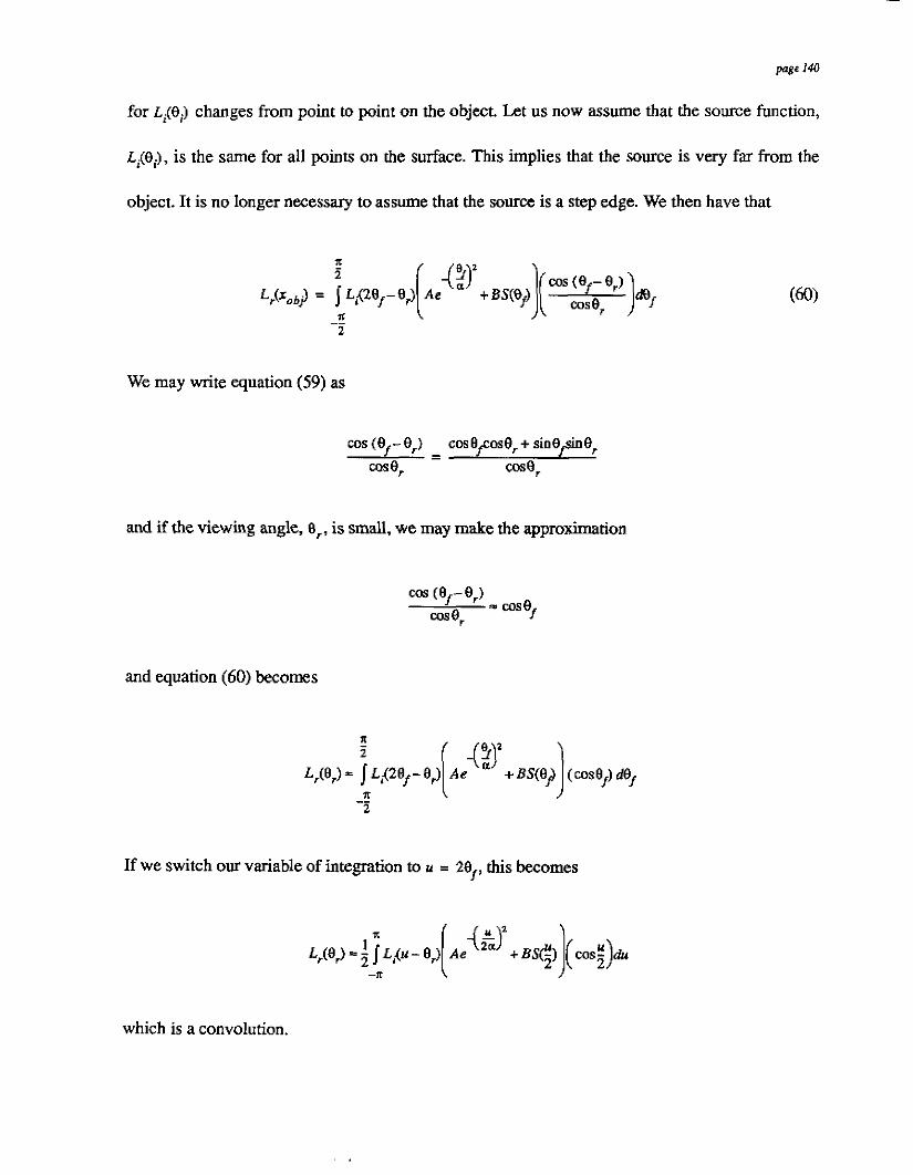
P8' 148
for Licei) changes from point to point on the object. Let us now assume that the source function,
Li(ei) , is the same for all points on the surface. This implies that the source is very far from the
object. It is no longer necessary to assume that the source is a step edge. We then have that
We may write equation (59) as
and if the viewing angle, e,, is small, we may make the approximation
and equation (60) becomes
If we switch our variable of integration to u = ZB,, this becomes
which is a convolution.

page 141
Convolution is a commonly used operation in the physical sciences and signal processing. In
order to solve a convolution equation, we may move into the Fourier domain by taking the Fou-
rier n a n s f m of both sides of the equation to yield
where 3 cf(r)) denotes the Fourier transform of the function flx) . We then solve for the weighted
sum by dividing by the transform of L,(u - e,) and taking the inverse Fourier transform to yield
Obviously, the form of the source function must be known.
There are a few problems with this method, none of which is insurmountable. First, if the Fou-
rier transform in the denominator takes on values with small or zero magnitude, the division
becomes unstable or even undefined. We may solve this problem by solving in the forward direc-
tion rather than by division, or by simply avoiding division for the small values and interpolating
the result from the rest of the function. Another problem with solving this type of equation is that
for computer applications, the Fourier bansform is found with the Fast Fourier Transform algo-
rithm. This algorithm imposes periodic boundary conditions on the data; in other words, it wraps
the data so that its beginning and end are the same value. This can cause problems, but there are
common techniques used in numerical analysis which circumvent any difficulties.
The convolution is one of the most used types of equations in image analysis. Therefore, it
should be easy to solve the reflected radiance equation with this method. We decided to use the

Volterra equation method of solution, however, since it did not involve the assumption that the
source is far from the surface, as does the convolution equation. We feel that it will be a fruitful
area of research for future investigators, however.