ROUGHING IT UP: INCLUDING JUMP COMPONENTS...

ROUGHING IT UP: INCLUDING JUMP COMPONENTS IN THEMEASUREMENT, MODELING, AND FORECASTING OF

RETURN VOLATILITY

Torben G. Andersen, Tim Bollerslev, and Francis X. Diebold*

Abstract—A growing literature documents important gains in asset returnvolatility forecasting via use of realized variation measures constructedfrom high-frequency returns. We progress by using newly developedbipower variation measures and corresponding nonparametric tests forjumps. Our empirical analyses of exchange rates, equity index returns, andbond yields suggest that the volatility jump component is both highlyimportant and distinctly less persistent than the continuous component,and that separating the rough jump moves from the smooth continuousmoves results in significant out-of-sample volatility forecast improve-ments. Moreover, many of the significant jumps are associated withspecific macroeconomic news announcements.

I. Introduction

VOLATILITY is central to asset pricing, asset alloca-tion, and risk management. In contrast to the estima-

tion of expected returns, which generally requires longtimespans of data, the results of Merton (1980) and Nelson(1992) suggest that volatility may be estimated arbitrarilywell through the use of sufficiently finely sampled high-frequency returns over any fixed time interval. However, theassumption of a continuous sample path diffusion underly-ing the theoretical results is invariably violated in practice.Thus, despite the increased availability of high-frequencydata for a host of different financial instruments, practicalcomplications have hampered the implementation of directhigh-frequency volatility modeling and filtering proce-dures.1

In response, Andersen and Bollerslev (1998), Andersen,Bollerslev, Diebold, and Labys (2001) (henceforth ABDL),Barndorff-Nielsen and Shephard (2002a,b), and Meddahi

(2002), among others, have recently advocated the use ofnonparametric realized volatility, or variation, measures toconveniently circumvent the data complications while re-taining most of the relevant information in the intraday datafor measuring, modeling, and forecasting volatilities overdaily and longer horizons. Indeed, the empirical results inABDL (2003) strongly suggest that simple models of real-ized volatility outperform the popular GARCH and relatedstochastic volatility models in out-of-sample forecasting.2

At the same time, recent parametric studies have sug-gested the importance of explicitly allowing for jumps, ordiscontinuities, in the estimation of specific stochastic vol-atility models and in the pricing of options and otherderivatives.3 In particular, it appears that many (log) priceprocesses are best described by a combination of a smoothand very slowly mean-reverting continuous sample pathprocess and a much less persistent jump component.4 Thusfar, however, the nonparametric realized volatility literaturehas paid comparatively little attention to jumps, and related,to distinguishing jump from nonjump movements.

Set against this backdrop, in the present paper we seek tofurther advance the nonparametric realized volatility ap-proach through the development of a practical nonparamet-ric procedure for separately measuring the continuous sam-ple path variation and the discontinuous jump part of thequadratic variation process. Our approach builds directly onthe new theoretical results in Barndorff-Nielsen and Shep-hard (2004a, 2006) involving so-called bipower variationmeasures constructed from the summation of appropriatelyscaled cross-products of adjacent high-frequency absolutereturns.5 Implementing these ideas empirically with morethan a decade of five-minute high-frequency returns for theDM/$ foreign exchange market, the S&P 500 market index,and the thirty-year U.S. Treasury yield, we shed new lighton the dynamics and comparative magnitudes of jumps

Received for publication March 30, 2004. Revision accepted for publi-cation April 17, 2006.

* Department of Finance, Northwestern University; Department of Eco-nomics, Duke University; and Department of Economics, University ofPennsylvania, respectively.

Earlier versions of this paper were circulated under the title “Some LikeIt Smooth, and Some Like It Rough: Disentangling Continuous and JumpComponents in Measuring, Modeling and Forecasting Asset Return Vol-atility.” Our research was supported by the National Science Foundation,the Guggenheim Foundation, and the Wharton Financial InstitutionsCenter. We are grateful to Olsen and Associates for generously supplyingtheir intraday exchange rate data. Xin Huang provided excellent researchassistance. We would also like to thank Federico Bandi, Michael Jo-hannes, Neil Shephard, George Tauchen, and two anonymous referees forhelpful comments, as well as seminar participants at the NBER/NSF TimeSeries Conference, the Montreal Realized Volatility Conference, the Aca-demia Sinica Conference on Analysis of High-Frequency Financial Dataand Market Microstructure, the Erasmus University Rotterdam Journal ofApplied Econometrics Conference, the Aarhus Econometrics Conference,the Seoul Far Eastern Meetings of the Econometric Society, the PortlandAnnual Meeting of the Western Finance Association, the NBER SummerInstitute, and the NYU Innovations in Financial Econometrics Confer-ence, as well as Baruch College, Nuffield College, Princeton, Toronto,UCLA, Wharton, and Uppsala Universities.

1 See, among others, Andersen and Bollerslev (1997), Dacorogna et al.(2001), Engle (2000), Russell and Engle (2005), and Rydberg and Shep-hard (2003).

2 These empirical findings are further corroborated by the analyticalresults for specific stochastic volatility models reported in Andersen,Bollerslev, and Meddahi (2004).

3 See, among others, Andersen, Benzoni, and Lund (2002), Bates (2000),Chan and Maheu (2002), Chernov, Gallant, Ghysels, and Tauchen (2003),Drost, Nijman, and Werker (1998), Eraker (2004), Eraker, Johannes, andPolson (2003), Johannes (2004), Johannes, Kumar, and Polson (1999),Maheu and McCurdy (2004), Khalaf, Saphores, and Bilodeau (2003), andPan (2002).

4 Earlier influential work on homoskedastic jump-diffusions includesMerton (1976), Ball and Torous (1983), Beckers (1981), and Jarrow andRosenfeld (1984). More recently, Jorion (1988) and Vlaar and Palm(1993) incorporated jumps in the estimation of discrete-time ARCH andGARCH models. See also the discussion in Das (2002).

5 This approach is distinctly different from the recent work of Aıt-Sahalia (2002), who relies on direct estimates of the transition densityfunction.

The Review of Economics and Statistics, November 2007, 89(4): 701–720© 2007 by the President and Fellows of Harvard College and the Massachusetts Institute of Technology

across the different markets. We also demonstrate importantgains in terms of volatility forecast accuracy by explicitlydifferentiating the jump and continuous sample path com-ponents. These gains obtain at daily, weekly, and evenmonthly forecast horizons. Our new HAR-RV-CJ forecast-ing model incorporating the jumps builds directly on theheterogenous AR model for the realized volatility, or HAR-RV model, due to Muller et al. (1997) and Corsi (2003), inwhich the realized volatility is parameterized as a linearfunction of the lagged realized volatilities over differenthorizons.

The paper proceeds as follows. In the next section webriefly review the relevant bipower variation theory. Insection III we describe our high-frequency data, extract apreliminary measure of jumps, and describe their features.In section IV we describe the HAR-RV volatility forecastingmodel, modify it to allow and control for jumps (producingour HAR-RV-J model), and assess its empirical perfor-mance. In section V we significantly refine the jump esti-mator by shrinking it toward zero in a fashion motivated byrecently developed powerful asymptotic theory, and byrobustifying it to market microstructure noise (as motivatedby the extensive simulation evidence in Huang andTauchen, 2005). We then illustrate that many of the jumpsso identified are associated with macroeconomic news. Insection VI we build a more refined model that makes fulluse our refined jump estimates by incorporating jump andnonjump components separately. The new model (HAR-RV-CJ) includes the earlier HAR-RV-J as a special and poten-tially restrictive case and produces additional forecast en-hancements. We conclude in section VII with severalsuggestions for future research.

II. Theoretical Framework

Let p(t) denote a logarithmic asset price at time t. Thecontinuous-time jump diffusion process traditionally used inasset pricing is conveniently expressed in stochastic differ-ential equation (sde) form as

dp�t� � ��t�dt � ��t�dW�t� � ��t�dq�t�,(1)

0 � t � T,

where �(t) is a continuous and locally bounded variationprocess, �(t) is a strictly positive stochastic volatility pro-cess with a sample path that is right continuous and haswell-defined left limits (allowing for occasional jumps involatility), W(t) is a standard Brownian motion, and q(t) isa counting process with (possibly) time-varying intensity�(t). That is, P[dq(t) � 1] � �(t)dt, where �(t) � p(t) p(t) refers to the size of the corresponding discrete jumpsin the logarithmic price process. The quadratic variation forthe cumulative return process, r(t) � p(t) p(0), is then

r, r�t � �0

t

�2�s�ds � �0�s�t

�2�s�, (2)

where by definition the summation consists of the q(t)squared jumps that occurred between time 0 and time t. Ofcourse, in the absence of jumps, or q(t) � 0, the summationvanishes and the quadratic variation simply equals theintegrated volatility of the continuous sample path compo-nent.

Several recent studies concerned with the direct estima-tion of continuous time stochastic volatility models havehighlighted the importance of explicitly incorporatingjumps in the price process along the lines of equation (1).6

Moreover, the specific parametric model estimates reportedin this literature have generally suggested that any dynamicdependence in the size or occurrence of the jumps is muchless persistent than the dependence in the continuous samplepath volatility process. Here we take a complementarynonparametric approach, squarely in the tradition of therealized volatility literature but specifically distinguishingjump from nonjump movements, relying on both the recentemergence of high-frequency data and powerful asymptotictheory.

A. High-Frequency Data, Bipower Variation, and Jumps

Let the discretely sampled -period returns be denoted byrt, � p(t) p(t ). For ease of notation we normalizethe daily time interval to unity and label the correspondingdiscretely sampled daily returns by a single time subscript,rt�1 � rt�1,1. Also, we define the daily realized volatility, orvariation, by the summation of the corresponding 1/ high-frequency intradaily squared returns,7

RVt�1� � � �j�1

1/

rt�j � , 2 , (3)

where for notational simplicity and without loss of gener-ality 1/ is assumed to be an integer. Then, as emphasizedinAndersen and Bollerslev (1998),ABDL (2001), Barndorff-Nielsen and Shephard (2002a, b), and Comte and Renault(1998), among others, it follows directly by the theory ofquadratic variation that the realized variation convergesuniformly in probability to the increment of the quadraticvariation process as the sampling frequency of the underly-ing returns increases. That is,

RVt�1� � 3 �t

t�1

�2�s�ds � �t�s�t�1

�2�s�, (4)

for 3 0. Thus, in the absence of jumps the realizedvariation is consistent for the integrated volatility that fig-ures prominently in the stochastic volatility option pricing

6 See, among others, Andersen, Benzoni, and Lund (2002), Eraker,Johannes, and Polson (2003), Eraker (2004), Johannes (2004), and Jo-hannes, Kumar, and Polson (1999).

7 We will use the terms realized volatility and realized variation inter-changeably.

THE REVIEW OF ECONOMICS AND STATISTICS702

literature. This result, in part, motivates the modeling andforecasting procedures for realized volatilities advocated inABDL (2003). It is clear, however, that in general therealized volatility will inherit the dynamics of both thecontinuous sample path process and the jump process.Although this does not impinge upon the theoretical justi-fication for directly modeling and forecasting RVt�1( )through simple procedures that do not distinguish jump andnonjump contributions to volatility, it does suggest thatsuperior forecasting models may be constructed by sepa-rately measuring and modeling the two components inequation (4).

Building on this intuition, the present paper seeks toimprove on the predictive models developed in ABDL(2003) through the use of new and powerful asymptoticresults (for 3 0) of Barndorff-Nielsen and Shephard(2004a, 2006) that allow for separate (nonparametric) iden-tification of the two components of the quadratic variationprocess. Specifically, define the standardized realized bi-power variation as

BVt�1� � � �12 �

j�2

1/

�rt�j� , � �rt�� j1�� , �, (5)

where �1 � �(2/�) � E(�Z�) denotes the mean of theabsolute value of standard normally distributed randomvariable, Z. It is then possible to show that for 3 0,8

BVt�1� � 3 �t

t�1

�2�s�ds. (6)

Hence, as first noted by Barndorff-Nielsen and Shephard(2004a), combining the results in equations (4) and (6), thecontribution to the quadratic variation process due to thediscontinuities (jumps) in the underlying price process maybe consistently estimated (for 3 0) by

RVt�1� � � BVt�1� � 3 �t�s�t�1

�2�s�. (7)

This is the central insight on which the theoretical andempirical results of this paper build.

Of course, nothing prevents the estimates of the squaredjumps defined by the right side of equation (7) from becom-ing negative in a given finite ( � 0) sample. Thus,following the suggestion of Barndorff-Nielsen and Shep-hard (2004a), we truncate the actual empirical measure-ments at zero,

Jt�1� � � maxRVt�1� � � BVt�1� �, 0�, (8)

to ensure that all of the daily estimates are nonnegative.

III. Data and Summary Statistics

To highlight the generality of our empirical results relatedto the improved forecasting performance obtained by sep-arately measuring the contribution to the overall variationcoming from the discontinuous price movements, wepresent the results for three different markets. We begin thissection with a brief discussion of the data sources, followedby a summary of the most salient features of the resultingrealized volatility and jump series for each of three markets.

A. Data Description

We present the results for three markets: the foreignexchange spot market (DM/$), the equity futures market(U.S. S&P 500 index), and the interest rate futures market(thirty-year U.S. Treasury yield). The DM/$ volatilitiesrange from December 1986 through June 1999, for a total of3,045 daily observations. The underlying high-frequencyspot quotations were kindly provided by Olsen & Associatesin Zurich, Switzerland. This same series has been previ-ously analyzed in ABDL (2001, 2003). The S&P 500 vol-atility measurements are based on tick-by-tick transactionsprices from the Chicago Mercantile Exchange (CME) aug-mented with overnight prices from the GLOBEX automatedtrade execution system, from January 1990 through Decem-ber 2002. The T-bond volatilities are similarly constructedfrom tick-by-tick transactions prices for the thirty-year U.S.Treasury bond futures contract traded on the Chicago Boardof Trade (CBOT), again from January 1990 through De-cember 2002. After removing holidays and other inactivetrading days, we have a total of 3,213 observations for eachof the two futures markets.9 A more detailed description ofthe S&P and T-bond data is available in Andersen, Boller-slev, Diebold, and Vega (2005), where the same high-frequency data are analyzed from a very different perspec-tive. All of the volatility measures are based on linearlyinterpolated logarithmic five-minute returns, as in Muller et

8 Corresponding general asymptotic results for so-called realized powervariation measures have recently been established by Barndorff-Nielsenand Shephard (2003, 2004a); see also Barndorff-Nielsen, Graversen, andShephard (2004) for a survey of related results. In particular, it followsthat in general for 0 � p � 2 and 3 0,

RPVt�1� , p� � �p1 1p/ 2 �

j�1

1/

�rt�j � , �p 3 �t

t�1

�p�s�ds,

where �p � 2p/ 2�(1⁄2( p � 1))/�(1⁄2) � E(�Z�p). Hence, the impact ofthe discontinuous jump process disappears in the limit for the powervariation measures with 0 � p � 2. In contrast, RPVt�1( , p) divergesto infinity for p � 2, while RPVt�1( , 2) � RVt�1( ) converges to theintegrated volatility plus the sum of the squared jumps, as in equation (4).Related expressions for the conditional moments of different powers ofabsolute returns have also been utilized by Aıt-Sahalia (2004) in theformulation of a GMM-type estimator for specific parametric homoske-dastic jump-diffusion models.

9 We explicitly exclude all days with sequences of more than twentyconsecutive five-minute intervals of no new prices for the S&P 500, andforty consecutive five-minute intervals of no new prices for the T-bondmarket.

ROUGHING IT UP 703

al. (1990) and Dacorogna et al. (1993).10 For the foreignexchange market this results in a total of 1/ � 288high-frequency return observations per day, while the twofutures contracts are actively traded for 1/ � 97 five-minute intervals per day. For notational simplicity, we omitthe explicit reference to in the following, referring to thefive-minute realized volatility and jump measures definedby equations (3) and (8) as RVt and Jt, respectively.

B. Realized Volatilities and Jumps

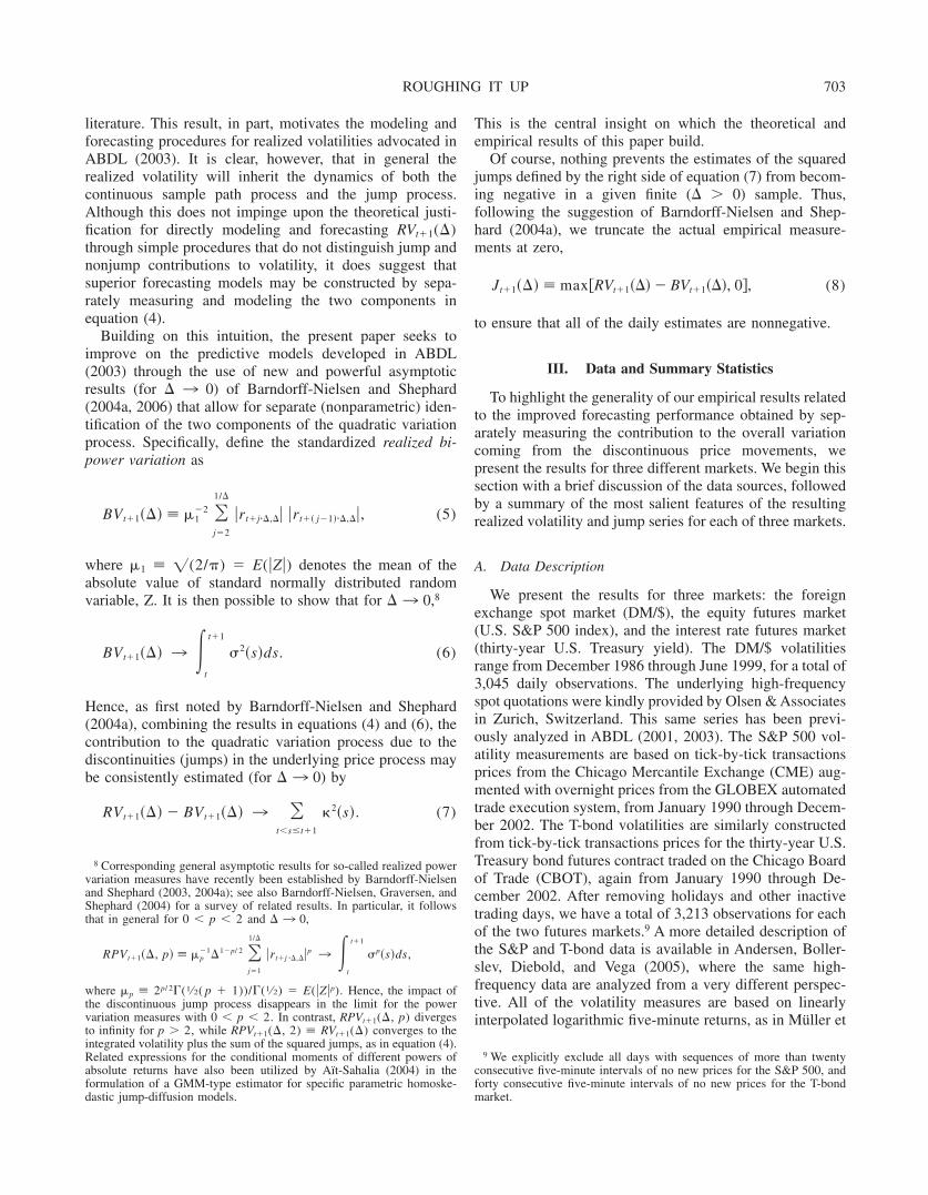
The first panels in figures 1A–C show the resulting threedaily realized volatility series in standard deviation form, orRVt

1/ 2. Each of the three series clearly exhibits a high degree

of own serial correlation. This is confirmed by the Ljung-Box statistics for up to tenth-order serial correlation re-ported in tables 1A–C equal to 5,714, 12,184, and 1,718,respectively. Similar results obtain for the realized variancesand logarithmic transformations reported in the first andthird columns in the tables. Comparing the volatility acrossthe three markets, the S&P 500 returns are the most volatile,followed by the exchange rate returns. Also, consistent withearlier evidence for the foreign exchange market in ABDL(2001), and related findings for individual stocks inAndersen, Bollerslev, Diebold, and Ebens (2001) and theS&P 500 in Deo, Hurvich, and Lu (2006) and Martens, vanDijk, and de Pooter (2004), the logarithmic standard devi-ations are generally much closer to being normally distrib-uted than are the raw realized volatility series. Hence, froma modeling perspective, the logarithmic realized volatilitiesare more amenable to the use of standard time seriesprocedures.11

The second panels in figures 1A–C display the separatemeasurements of the jump components (again in standarddeviation form) based on the truncated estimator in equation

10 To mitigate the impact of market microstructure frictions in theconstruction of unbiased and efficient realized volatility measurements, anumber of recent studies have proposed ways of “optimally” choosing (e.g., Aıt-Sahalia, Mykland, & Zhang, 2005; Bandi & Russell, 2004,2006), subsampling schemes (e.g., Zhang, Aıt-Sahalia, & Mykland, 2005;Zhang, 2004), prefiltering (e.g., Andreou & Ghysels, 2002; Areal &Taylor, 2002; Bollen & Inder, 2002; Corsi, Zumbach, Muller, & Da-corogna, 2001; Oomen, 2006), Fourier methods (Barucci & Reno, 2002;Malliavin & Mancino, 2002), or other kernel type estimators (e.g.,Barndorff-Nielsen, Hansen, Lunde, & Shephard, 2006; Hansen & Lunde,2006; Zhou, 1996). For now we simply follow ABDL (2000, 2001), alongwith most of the existing empirical literature, in the use of unweightedfive-minute returns for each of the three actively traded markets analyzedhere. However, we will return to a more detailed discussion of the marketmicrostructure issue and pertinent jump measurements in section V below.

11 Modeling and forecasting log volatility also has the virtue of auto-matically imposing nonnegativity of fitted and forecasted volatilities.

FIGURE 1.—(A) DAILY DM/$ REALIZED VOLATILITIES AND JUMPS; (B) DAILY S&P 500 REALIZED VOLATILITIES AND JUMPS

0.00.51.01.52.02.5

1987 1989 1991 1993 1995 1997 1999

0.00.51.01.52.02.5

1987 1989 1991 1993 1995 1997 1999

0

5

10

15

1987 1989 1991 1993 1995 1997 1999

0.00.51.01.52.02.5

1987 1989 1991 1993 1995 1997 1999

0123456

1990 1992 1994 1996 1998 2000 2002

0123456

1990 1992 1994 1996 1998 2000 2002

0

5

10

15

1990 1992 1994 1996 1998 2000 2002

0123456

1990 1992 1994 1996 1998 2000 2002

Key: The top panel shows daily realized volatility in standard deviation form, or RVt1/ 2. The second panel graphs the jump component defined in equation (8), Jt

1/ 2. The third panel shows the Z1,t( ) statistic, withthe 0.999 significance level indicated by the horizontal line. The bottom panel graphs the significant jumps corresponding to � � 0.999, or Jt,0.999

1/ 2 . See the text for details.


(8).12 As is evident from the figures, many of the largestrealized volatilities are directly associated with jumps in theunderlying price process. Some of the largest jumps in theDM/$ market occurred during the earlier 1986–88 part ofthe sample, while the size of the jumps for the S&P 500 hasincreased significantly over the most recent 2001–02 period.In contrast, the size of the jumps in the T-bond market seemto be much more evenly distributed throughout the sample.Overall, both the size and occurrence of jumps appear to bemuch more predictable for the S&P 500 than for the othertwo markets.

These visual observations are readily confirmed by thestandard Ljung-Box portmanteau statistics for up to tenth-order serial correlation in the Jt, Jt

1/ 2, and log ( Jt � 1)series reported in the last three columns in tables 1A–C.It is noteworthy that although the Ljung-Box statistics forthe jumps are generally significant at conventional sig-nificance levels (especially for the jumps expressed instandard deviation or logarithmic form), the actual values

are markedly lower than the corresponding test statisticsfor the realized volatility series reported in the first threecolumns. This indicates decidedly less own dynamicdependence in the portion of the overall quadratic vari-ation originating from the discontinuous sample pathprice process compared to the dynamic dependence in thecontinuous sample path price movements. The numbersin the table also indicate that the jumps are relativelyleast important for the DM/$ market, with the mean of theJt series accounting for 0.072 of the mean of RVt, whilethe same ratios for the S&P 500 and T-bond marketsequal 0.144 and 0.126, respectively.

Motivated by these observations, we now put the idea ofseparately measuring the jump component to work in theconstruction of new and simple-to-implement realized vol-atility forecasting models. More specifically, we followABDL (2003) in directly estimating a set of time seriesmodels for each of the different realized volatility measuresin tables 1A–C; i.e., RVt, RVt

1/ 2, and log (RVt). Then, inorder to assess the added value of separately measuring thejump component in forecasting the realized volatilities, wesimply include the raw Jt, Jt

1/ 2, and log ( Jt � 1) jump seriesas additional explanatory variables in the various forecast-ing regressions.

IV. Accounting for Jumps in Realized VolatilityModeling and Forecasting

A number of empirical studies have argued for the im-portance of long-memory dependence in financial marketvolatility. Several different parametric ARCH and stochasticvolatility formulations have also been proposed in the liter-ature for capturing this phenomenon (e.g., Andersen &Bollerslev, 1997; Baillie, Bollerslev, & Mikkelsen, 1996;Breidt, Crato, & de Lima, 1998; Dacorogna et al., 2001;Ding, Granger, & Engle, 1993; Robinson, 1991). Thesesame empirical observations have similarly motivated theestimation of long-memory type ARFIMA models for real-ized volatilities in ABDL (2003), Areal and Taylor (2002),Deo, Hurvich, and Lu (2006), Koopman, Jungbacker, andHol (2005), Martens, van Dijk, and de Pooter (2004), Pong,Shackleton, Taylor, and Xu (2004), and Thomakos andWang (2003), among others.

Here we eschew such complicated fractionally integratedlong-memory formulations and rely instead on the simple-to-estimate HAR-RV class of volatility models proposed byCorsi (2003). The HAR-RV formulation is based on astraightforward extension of the so-called HeterogeneousARCH, or HARCH, class of models analyzed by Muller etal. (1997), in which the conditional variance of the dis-cretely sampled returns is parameterized as a linear functionof the lagged squared returns over the identical returnhorizon together with the squared returns over longer and/or

12 The difference between the daily realized variation and bipowervariation measures result in negative estimates for the squared daily jumpson 30.6%, 27.9%, and 18.3% of the days for each of the three markets,respectively. As discussed below, in the absence of jumps, the differenceshould be negative asymptotically ( 3 0) for half of the days in thesample.

FIGURE 1C.—DAILY U.S. T-BOND REALIZED VOLATILITIES AND JUMPS

0.00.40.81.21.62.0

1990 1992 1994 1996 1998 2000 2002

0.0

0.5

1.0

1.5

2.0

1990 1992 1994 1996 1998 2000 2002

0

5

10

15

1990 1992 1994 1996 1998 2000 2002

0.0

0.5

1.0

1.5

2.0

1990 1992 1994 1996 1998 2000 2002

Key: The top panel shows daily realized volatility in standard deviation form, or RVt1/ 2. The second

panel graphs the jump component defined in equation (8), Jt1/ 2. The third panel shows the Z1,t( ) statistic,

with the 0.999 significance level indicated by the horizontal line. The bottom panel graphs the significantjumps corresponding to � � 0.999, or Jt,0.999

1/ 2 . See the text for details.

ROUGHING IT UP 705

shorter return horizons.13 Although the HAR structure doesnot formally possess long memory, the mixing of relativelyfew volatility components is capable of reproducing a re-markably slow volatility autocorrelation decay that is al-most indistinguishable from that of a hyperbolic (long-memory) pattern over most empirically relevant forecasthorizons.14

A. The HAR-RV-J Model

To define the HAR-RV model, let the multiperiod nor-malized realized variation, defined by the sum of the corre-sponding one-period measures, be denoted by

RVt,t�h � h1RVt�1 � RVt�2 � · · · � RVt�h�, (9)

where h � 1, 2, . . . . Note that, by definition RVt,t�1 �RVt�1. Also, provided that the expectations exist,E(RVt,t�h) � E(RVt�1) for all h. For ease of reference, wewill refer to these normalized measures for h � 5 and h �22 as the weekly and monthly volatilities, respectively. Thedaily HAR-RV model of Corsi (2003) may then be ex-pressed as15

RVt�1 � �0 � �DRVt � �WRVt5,t � �MRVt22,t � εt�1,

(10)

where t � 1, 2, . . . , T. Of course, realized volatilities overother horizons could easily be included as additional ex-planatory variables on the right side of the regression

13 Muller et al. (1997) heuristically motivate the HARCH model throughthe existence of distinct groups of traders with different investmenthorizons.

14 Mixtures of low-order ARMA models have similarly been used inapproximating and forecasting long-memory dependence in the condi-tional mean by Basak, Chan, and Palma (2001), Cox (1991), Hsu andBreidt (2003), Man (2003), O’Connell (1971), and Tiao and Tsay (1994),among others. The component GARCH model in Engle and Lee (1999)and the multifactor continuous time stochastic volatility model in Gallant,Hsu, and Tauchen (1999) are both motivated by similar considerations; seealso the discussion of the related multifractal regime-switching models inCalvet and Fisher (2001, 2002).

15 The time series of realized volatilities in this and all of the subsequentHAR-RV regressions are implicitly assumed to be stationary. Formal testsfor a unit root in RVt�1 easily reject the null hypothesis of nonstationarityfor each of the three markets. Also, the standard log-periodogram esti-mates of the degree of fractional integration in RVt�1 equal 0.347, 0.383,and 0.437, respectively, with a theoretical asymptotic standard error of0.087.

TABLE 1A.—SUMMARY STATISTICS FOR DAILY DM/$ REALIZED VOLATILITIES AND JUMPS

RVt RVt1/2 log (RVt) Jt Jt

1/2 log (Jt � 1)

Mean 0.508 0.670 0.915 0.037 0.129 0.033St. dev. 0.453 0.245 0.657 0.110 0.142 0.072Skewness 3.925 1.784 0.408 16.52 2.496 7.787Kurtosis 26.88 8.516 3.475 434.2 18.20 108.5Min. 0.052 0.227 2.961 0.000 0.000 0.000Max. 5.245 2.290 1.657 3.566 1.889 1.519LB10 3,786 5,714 7,060 16.58 119.4 63.19

TABLE 1B.—SUMMARY STATISTICS FOR DAILY S&P 500 REALIZED VOLATILITIES AND JUMPS


1/2 log (Jt � 1)

Mean 1.137 0.927 0.400 0.164 0.232 0.097St. dev. 1.848 0.527 0.965 0.964 0.332 0.237Skewness 7.672 2.545 0.375 20.68 5.585 6.386Kurtosis 95.79 14.93 3.125 551.9 59.69 59.27Min. 0.058 0.240 2.850 0.000 0.000 0.000Max. 36.42 6.035 3.595 31.88 5.646 3.493LB10 5,750 12,184 15,992 558.0 1,868 2,295

TABLE 1C.—SUMMARY STATISTICS FOR DAILY U.S. T-BOND REALIZED VOLATILITIES AND JUMPS


1/2 log (Jt � 1)

Mean 0.286 0.506 1.468 0.036 0.146 0.033St. dev. 0.222 0.173 0.638 0.069 0.120 0.055Skewness 3.051 1.352 0.262 8.732 1.667 5.662Kurtosis 20.05 6.129 3.081 144.6 10.02 57.42Min. 0.026 0.163 3.633 0.000 0.000 0.000Max. 2.968 1.723 1.088 1.714 1.309 0.998LB10 1,022 1,718 2,238 20.53 34.10 26.95

Key: The first six rows in each of the panels report the sample mean, standard deviation, skewness, and kurtosis, along with the sample minimum and maximum. The rows labeled LB10 give the Ljung-Box teststatistic for up to tenth-order serial correlation. The daily realized volatilities and jumps for the DM/$ in panel A are constructed from five-minute returns spanning the period from December 1986 through June1999, for a total of 3,045 daily observations. The daily realized volatilities and jumps for the S&P 500 and U.S. T-bonds in panels B and C are based on five-minute returns from January 1990 through December2002, for a total of 3,213 observations.


equation, but the daily, weekly, and monthly measuresemployed here afford a natural economic interpretation.16

This HAR-RV model for one-day volatilities extendsstraightforwardly to longer horizons, RVt,t�h. Moreover,given the separate nonparametric measurements of the jumpcomponent discussed above, the corresponding time seriesis readily included as an additional explanatory variable,resulting in the new HAR-RV-J model,

RVt,t�h � �0 � �DRVt � �WRVt5,t � �MRVt22,t

� �JJt � εt,t�h.(11)

With observations every period and longer forecast horizons,or h � 1, the error term will generally be serially correlated upto (at least) order h 1. This will not affect the consistency ofthe regression coefficient estimates, but the correspondingstandard errors of the estimates obviously need to be adjusted.In the results discussed below, we rely on the Bartlett/Newey-West heteroskedasticity consistent covariance matrix estimatorwith 5, 10, and 44 lags for the daily (h � 1), weekly (h � 5),and monthly (h � 22) regression estimates, respectively.

Turning to the results reported in the first three columnsin tables 2A–C, the estimates for �D, �W, and �M confirmthe existence of highly persistent volatility dependence.Interestingly, the relative importance of the daily volatilitycomponent decreases from the daily to the weekly to themonthly regressions, whereas the monthly volatility com-ponent tends to be relatively more important for the longer-run monthly regressions. Importantly, the estimates of thejump component, �J, are systematically negative across allmodels and markets, and with few exceptions, overwhelm-ingly significant.17 Thus, whereas the realized volatilitiesare generally highly persistent, the impact of the laggedrealized volatility is significantly reduced by the jumpcomponent. For instance, for the daily DM/$ realized vol-atility a unit increase in the daily realized volatility impliesan average increase in the volatility on the following day of0.430 � 0.196/5 � 0.244/22 � 0.480 for days where Jt �0, whereas for days in which part of the realized volatilitycomes from the jump component the increase in the vola-tility on the following day is reduced by 0.486 times thejump component. In other words, if the realized volatility isentirely attributable to jumps, it carries no predictive powerfor the following day’s realized volatility. Similarly for theother two markets: the combined impact of a jump forforecasting the next day’s realized volatility equals 0.341 �0.485/5 � 0.165/22 0.472 � 0.027 and 0.074 �0.317/5 � 0.358/22 0.152 � 0.002, respectively.

Comparing the R2’s of the HAR-RV-J models to the R2’sof the “standard” HAR model reported in the last row, inwhich the jump component is absent and the realizedvolatilities on the right side but not the left side of equation(11) are replaced by the corresponding lagged squared daily,weekly, and monthly returns clearly highlights the addedvalue of the high-frequency data. Although the coefficientestimates of the �D, �W, and �M coefficients in the “stan-dard” HAR models (available upon request) generally alignfairly closely with those of the HAR-RV-J models reportedin the tables, the explained variation is systematicallylower.18 Importantly, the gains afforded by the use of thehigh-frequency-based realized volatilities are not restrictedto the daily and weekly horizons. In fact, the longer-runmonthly forecasts result in the largest relative increases inthe R2’s, with those for the S&P 500 and T-bonds tripling forthe HAR-RV-J models relative to those from the HARmodels based on the coarser daily, weekly, and monthlysquared returns. These large gains in forecast accuracythrough the use of realized volatilities are, of course, en-tirely consistent with the earlier empirical evidence inABDL (2003), Bollerslev and Wright (2001), and Martens(2002), among others, and further corroborated by the analyt-ical results of Andersen, Bollerslev, and Meddahi (2004).

B. Nonlinear HAR-RV-J Models

Practical use of volatility models and forecasts ofteninvolves standard deviations as opposed to variances. Thesecond set of columns in tables 2A–C thus reports theparameter estimates and R2’s of the corresponding HAR-RV-J model cast in standard deviation form,

�RVt,t�h�1/ 2 � �0 � �DRVt

1/ 2��W�RVt5,t�1/ 2

��M�RVt22,t�1/ 2��JJt

1/ 2 � εt,t�h.(12)

The qualitative features and ordering of the different param-eter estimates are generally the same as for the varianceformulation in equation (11). In particular, the estimates for�J are systematically negative. Similarly, the R2’s indicatequite dramatic gains for the high-frequency-based HAR-RV-J model relative to the standard HAR model. The morerobust volatility measurements provided by the standarddeviations also result in higher R2’s than for the variance-based models reported in the first three columns.19

As noted in table 1 above, the logarithmic daily real-ized volatilities are approximately unconditionally normally

16 Related mixed data sampling, or MIDAS in the terminology ofGhysels, Santa-Clara, and Valkanov (2004), regressions have recentlybeen estimated by Ghysels, Santa-Clara, and Valkanov (2006).

17 Note that nothing prevents the forecasts of the realized volatilitiesfrom the HAR-RV-J model with �J � 0 from becoming negative. We didnot find this to be a problem for any of our in-sample model estimates,however. A more complicated multiplicative error structure, along thelines of Engle (2002) and Engle and Gallo (2006), could be employed toensure positivity of the conditional expectations.

18 Note that although the relative magnitudes of the R2’s for a givenvolatility series are directly comparable across the two models, as dis-cussed in Andersen, Bollerslev, and Meddahi (2005), the measurementerrors in the left-hand-side realized volatility invariably result in a sys-tematic downward bias in the reported R2’s vis-a-vis the inherent predict-ability in the true latent quadratic variation process.

19 The R2 � 0.431 for the daily HAR-RV-J model for the DM/$ realizedvolatility series in the fourth column in table 2A also exceeds thecomparable in-sample one-day-ahead R2 � 0.355 for the long-memoryVAR model reported in ABDL (2003).

ROUGHING IT UP 707

TABLE 2A.—DAILY, WEEKLY, AND MONTHLY DM/$ HAR-RV-J REGRESSIONS

RVt,t�h � �0 � �DRVt � �WRVt5,t � �MRVt22,t � �JJt � εt,t�h

(RVt,t�h)1/2 � �0 � �DRVt1/2 � �W(RVt5,t)1/2 � �M(RVt22,t)1/2 � �JJt

1/2 � εt,t�h

log (RVt,t�h) � �0 � �D log (RVt) � �W log (RVt5,t) � �M log (RVt22,t) � �J log (Jt � 1) � εt,t�h

h

RVt,t�h (RVt,t�h)1/2 log (RVt,t�h)

1 5 22 1 5 22 1 5 22

�0 0.083 0.132 0.231 0.096 0.159 0.293 0.122 0.142 0.269(0.015) (0.018) (0.025) (0.015) (0.021) (0.034) (0.021) (0.030) (0.048)

�D 0.430 0.222 0.110 0.392 0.216 0.124 0.408 0.252 0.162(0.043) (0.040) (0.022) (0.033) (0.028) (0.020) (0.030) (0.029) (0.027)

�W 0.196 0.216 0.218 0.248 0.264 0.243 0.271 0.265 0.221(0.063) (0.055) (0.043) (0.046) (0.050) (0.040) (0.042) (0.051) (0.039)

�M 0.244 0.323 0.225 0.223 0.296 0.219 0.212 0.284 0.226(0.061) (0.068) (0.062) (0.041) (0.056) (0.063) (0.036) (0.054) (0.065)

�J 0.486 0.297 0.166 0.103 0.047 0.026 0.762 0.590 0.395(0.096) (0.070) (0.056) (0.039) (0.031) (0.029) (0.161) (0.176) (0.178)

RHAR-RV-J2 0.364 0.417 0.353 0.431 0.472 0.386 0.476 0.502 0.407

RHAR2 0.252 0.261 0.215 0.261 0.272 0.225 0.160 0.159 0.138

Key: The table reports the OLS estimates for daily (h � 1) and overlapping weekly (h � 5) and monthly (h � 22) HAR-RV-J volatility forecast regressions. The realized volatilities and jumps are constructedfrom five-minute returns spanning the period from December 1986 through June 1999, for a total of 3,045 daily observations. The standard errors reported in parentheses are based on a Newey-West/Bartlett correctionallowing for serial correlation of up to order 5 (h � 1), 10 (h � 5), and 44 (h � 22), respectively. The last two rows labeled RHAR-RV-J

2 and RHAR2 are for the HAR-RV-J model and a “standard” HAR model with

no jumps and with the realized volatilities on the right side of the regression replaced with the corresponding lagged daily, weekly, and monthly squared returns.

TABLE 2B.—DAILY, WEEKLY, AND MONTHLY S&P 500 HAR-RV-J REGRESSIONS



1/2 � εt,t�h


h


1 5 22 1 5 22 1 5 22

�0 0.088 0.186 0.387 0.060 0.102 0.205 0.065 0.001 0.022(0.054) (0.066) (0.074) (0.020) (0.030) (0.038) (0.015) (0.019) (0.036)

�D 0.341 0.220 0.109 0.375 0.262 0.169 0.348 0.235 0.164(0.094) (0.064) (0.040) (0.041) (0.038) (0.029) (0.028) (0.025) (0.024)

�W 0.485 0.430 0.287 0.354 0.395 0.291 0.329 0.363 0.260(0.111) (0.097) (0.093) (0.064) (0.067) (0.071) (0.041) (0.050) (0.049)

�M 0.165 0.220 0.279 0.239 0.270 0.357 0.285 0.334 0.444(0.067) (0.079) (0.088) (0.040) (0.058) (0.069) (0.031) (0.046) (0.054)

�J 0.472 0.228 0.075 0.213 0.134 0.054 0.260 0.187 0.105(0.102) (0.078) (0.067) (0.051) (0.041) (0.046) (0.062) (0.064) (0.080)

RHAR-RV-J2 0.415 0.569 0.474 0.604 0.697 0.634 0.693 0.761 0.727

RHAR2 0.248 0.239 0.159 0.322 0.320 0.275 0.197 0.219 0.218

Key: The table reports the OLS estimates for daily (h � 1) and overlapping weekly (h � 5) and monthly (h � 22) HAR-RV-J volatility forecast regressions. The realized volatilities and jumps are constructedfrom five-minute returns spanning the period from January 1990 through December 2002, for a total of 3,213 daily observations. The standard errors reported in parentheses are based on a Newey-West/Bartlettcorrection allowing for serial correlation of up to order 5 (h � 1), 10 (h � 5), and 44 (h � 22), respectively. The last two rows labeled RHAR-RV-J

2 and RHAR2 are for the HAR-RV-J model and a “standard” HAR

model with no jumps and with the realized volatilities on the right side of the regression replaced with the corresponding lagged daily, weekly, and monthly squared returns.

TABLE 2C.—DAILY, WEEKLY, AND MONTHLY U.S. T-BOND HAR-RV-J REGRESSIONS



1/2 � εt,t�h


h


1 5 22 1 5 22 1 5 22

�0 0.077 0.088 0.126 0.118 0.152 0.222 0.353 0.323 0.473(0.012) (0.013) (0.017) (0.017) (0.021) (0.031) (0.044) (0.051) (0.080)

�D 0.074 0.084 0.044 0.066 0.082 0.044 0.104 0.100 0.063(0.031) (0.016) (0.011) (0.026) (0.014) (0.009) (0.024) (0.015) (0.012)

�W 0.317 0.217 0.160 0.319 0.215 0.162 0.324 0.206 0.154(0.050) (0.043) (0.040) (0.045) (0.039) (0.036) (0.043) (0.039) (0.032)

�M 0.358 0.416 0.373 0.369 0.429 0.388 0.379 0.440 0.395(0.056) (0.055) (0.070) (0.046) (0.051) (0.068) (0.046) (0.053) (0.070)

�J 0.152 0.202 0.140 0.047 0.062 0.042 0.869 0.693 0.545(0.099) (0.042) (0.034) (0.032) (0.018) (0.015) (0.240) (0.129) (0.123)

RHAR-RV-J2 0.130 0.308 0.340 0.171 0.332 0.360 0.200 0.351 0.379

RHAR2 0.067 0.128 0.105 0.072 0.117 0.093 0.025 0.042 0.035

Key: The table reports the OLS estimates for daily (h � 1) and overlapping weekly (h � 5) and monthly (h � 22) HAR-RV-J volatility forecast regressions. The realized volatilities and jumps are constructedfrom five-minute returns spanning the period from January 1990 through December 2002, for a total of 3,213 daily observations. The standard errors reported in parentheses are based on a Newey-West/Bartlettcorrection allowing for serial correlation of up to order 5 (h � 1), 10 (h � 5), and 44 (h � 22), respectively. The last two rows labeled RHAR-RV-J

2 and RHAR2 are for the HAR-RV-J model and a “standard” HAR

model with no jumps and with the realized volatilities on the right side of the regression replaced with the corresponding lagged daily, weekly, and monthly squared returns.


distributed for each of the three markets. This empiricalregularity motivated ABDL (2003) to model the logarithmicrealized volatilities, in turn allowing for the use of standardnormal distribution theory and related mixture models.20

Guided by this same idea, we report in the last threecolumns of tables 2A–C the estimates of the logarithmicHAR-RV-J model,

log �RVt,t�h� � �0 � �D log �RVt� � �W log �RVt,t5�

� �M log �RVt,t22�

� �J log �Jt � 1� � εt,t�h.

(13)

The estimates are again directly in line with those of theHAR-RV-J models for RVt,t�h and (RVt,t�h)1/ 2 discussedearlier. In particular, the �D coefficients are generally thelargest in the daily models, the �W’s are the most importantin the weekly models, and the �M’s in the monthly models.At the same time, the negative estimates of the �J coeffi-cients temper the persistency in the forecasts, suggestingthat jumps in the price processes tend to be associated withshort-lived bursts in volatility.

V. Shrinkage Estimation and MicrostructureNoise Correction

The empirical results discussed thus far rely on the simplenonparametric jump estimates defined by the differencebetween the realized volatility and the bipower variation. Asdiscussed in section II, the theoretical justification for thosemeasurements is based on the notion of increasingly finersampled returns, or 3 0. Of course, any practical imple-mentation with a fixed sampling frequency, or � 0, isinvariably subject to measurement error. The nonnegativitytruncation in equation (8) alleviates part of this finite-sample problem by eliminating theoretically infeasible neg-ative estimates for the squared jumps. However, the result-ing Jt

1/ 2 series depicted in figures 1A–C arguably alsoexhibit an unreasonably large number of nonzero smallpositive values. It may be desirable to treat these smalljumps as measurement errors, or part of the continuoussample path variation process, associating only large valuesof RVt( ) BVt( ) with the jump component. The nextsubsection provides a theoretical framework for doing so.

A. Asymptotic Distribution Theory

The distributional results developed in Barndorff-Nielsenand Shephard (2004a, 2006) and extended in Barndorff-

Nielsen, Graversen, Jacod, et al. (2006) imply that, undersufficient regularity, frictionless market conditions and inthe absence of jumps in the price path,

1/ 2RVt�1� � � BVt�1� �

��14 � 2�1

2 � 5� �t

t�1

�4�s�ds�1/ 2

f N�0, 1�,

(14)

for 3 0. Hence, an abnormally large value of thisstandardized difference between RVt�1( ) and BVt�1( ) isnaturally interpreted as evidence in favor of a “significant”jump over the [t, t � 1] time interval. Of course, theintegrated quarticity that appears in the denominator needsto be estimated in order to actually implement this statistic.In parallel to the arguments underlying the robust estimationof the integrated volatility by the realized bipower variation,it is possible to show that even in the presence of jumps, theintegrated quarticity may be consistently estimated by thenormalized sum of the product of n � 3 adjacent absolutereturns raised to the power of 4/n. In particular, on definingthe standardized realized tripower quarticity measure,

TQt�1� �

� 1�4/33 �

j�3

1/

�rt�j � , �4/3�rt�� j1�� , �4/3�rt�� j2�� , �4/3,

(15)

where �4/3 � 22/3 � �(7/6) � �(1⁄2)1 � E(�Z�4/3). Itfollows that for 3 0,

TQt�1� � f �t

t�1

�4�s�ds. (16)

Combining the results in equations (14)–(16), the “signifi-cant” jumps may therefore be identified by comparingrealizations of the feasible test statistics,21

20 This same transformation has subsequently been used for other mar-kets by Deo, Hurvich, and Lu (2006), Koopman, Jungbacker, and Hol(2005), and Martens, van Dijk, and de Pooter (2004) among others. Ofcourse, the log-normal distribution isn’t closed under temporal aggrega-tion. Thus, if the daily logarithmic realized volatilities are normallydistributed, the weekly and monthly volatilities can not also be log-normally distributed. However, as argued by Barndorff-Nielsen and Shep-hard (2002a) and Forsberg and Bollerslev (2002), the log-normal volatilitydistributions may be closely approximated by Inverse Gaussian distribu-tions, which are formally closed under temporal aggregation.

21 Similar results were obtained by using the robust realized quad-powerquarticity measure advocated in Barndorff-Nielsen and Shephard (2004a,2006),

QQt�1� � � 1�14 �

j�4

1/

�rt�j � , � �rt�� j1�� , �rt�� j2�� , .�rt�� j3�� , �.

Note, however, that the realized quarticity,

RQt�1� � � RPVt�1� , 4� � 1�41 �

j�1

1/

rt�j � , 4 ,

used in estimating the integrated quarticity by Barndorff-Nielsen andShephard (2002a) and Andersen, Bollerslev, and Meddahi (2005) is notconsistent in the presence of jumps, which in turn would result in acomplete loss of power for the corresponding test statistic obtained byreplacing TQt�1( ) in equation (17) with RQt�1( ).

ROUGHING IT UP 709

Wt�1� � � 1/ 2RVt�1� � � BVt�1� �

��14 � 2�1

2 � 5�TQt�1� ��1/ 2 ,

(17)

to a standard normal distribution.The extensive simulation-based evidence for specific

parametric continuous time diffusions reported in Huangand Tauchen (2005) suggests that the Wt�1( ) statisticdefined in equation (17) tends to over-reject the null hy-pothesis of no jumps for large critical values. At the sametime, following the approach advocated by Barndorff-Nielsen and Shephard (2004b), different variance stabilizingtransforms for the joint asymptotic distribution of the real-ized volatility and bipower variation measures generallyproduce test statistics with improved finite-sample perfor-mance. In particular, on applying the delta rule to the jointbivariate distribution, Huang and Tauchen (2005) find thatthe ratio-statistic,

Zt�1� � � 1/ 2

�RVt�1� � � BVt�1� ��RVt�1� �1

��14 � 2�1

2 � 5� max �1, TQt�1� �BVt�1� �2��1/ 2 ,

(18)

where the max adjustment follows by a Jensen’s inequalityargument as in Barndorff-Nielsen and Shephard (2004b), isvery closely approximated by a standard normal distributionthroughout its entire support in samples of the size relevanthere.22 Moreover, they find that the ratio-statistic in equation(18) also has reasonable power against several empiricallyrealistic calibrated stochastic volatility jump diffusion mod-els.

Hence we naturally identify the “significant” jumps bythe realizations of Zt�1( ) in excess of some critical value,say ��,

Jt�1,�� IZt�1� � � �� RVt�1� � (19)

BVt�1� �],

where I[�] denotes the indicator function.23 To ensure thatthe estimated continuous sample path component variationand jump variation sum to the total realized variation, weestimate the former component as the residual,

Ct�1,�� IZt�1� � � �� RVt�1� � (20)

�I[Zt�1( )��]�BVt�1( ).

Note that for �� 0, the definitions in equations (19) and(20) automatically guarantee that both Jt�1,�( ) andCt�1,�( ) are positive.24 Of course, the nonnegativity trun-cation imposed in equation (8) underlying the empiricaljump measurements employed in the preceding two sectionscorresponds directly to � � 0.5, or Jt,0.5.

B. Market Microstructure Noise

As already discussed in section IIIA, a host of practicalmarket microstructure frictions, including the use of discreteprice grid points and bid-ask spreads, invariably rendersfictitious the assumption of a continuously observed loga-rithmic price process following a semimartigale. Hence,following Aıt-Sahalia, Mykland, and Zhang (2005), Bandiand Russell (2006), and Zhang, Mykland, and Aıt-Sahalia(2005), among others, assume that the observed price pro-cess is “contaminated” by a market microstructure noisecomponent, say p(t) � p*(t) � v(t), where p*(t) refers tothe true (latent) semimartingale logarithmic price processthat would obtain in the absence of any frictions, while v(t)denotes an i.i.d. white-noise component.25 The discretelysampled -period observed returns,

rt, � p*�t� � p*�t � � � v�t� � v�t � � (21)

�r*t, � �t, ,

then equal the true (latent) returns plus the first-ordermoving-average process, �t, . Assuming that the varianceof v(t) does not depend upon , the noise term willeventually (for 3 0) dominate the contribution to theoverall realized variation in equation (3) coming from thesquared true (latent) high-frequency returns, formally ren-dering RVt�1( ) inconsistent as a measure of the quadraticvariation of p*(t). In practice, the impact of the marketmicrostructure noise is most easily controlled through thechoice of . Our choice of a five-minute sampling fre-quency for the very active markets analyzed here is moti-vated by this bias-variance tradeoff, as the bias in therealized variation measure in equation (3) appears to largelyvanish at this frequency.

By analogous arguments, the noise term will generallyresult in an upward bias in the new bipower variationmeasure in equation (5) for “too small,” as E(�r*t, �) �E(�r*t, � �t, �). The first-order serial correlation in �t,

further implies that any two adjacent observed returns, sayrt�j � , and rt�( j1) � , , will be serially correlated. In com-parison to the realized variation measure based on the sum

22 In an earlier version of this paper, we relied on the log-based statistic,

Ut�1� � � 1/ 2log �RVt�1� �� log �BVt�1� ��

��14 � 2�1

2 � 5�TQt�1� �BVt�1� �2�1/ 2 ,

which produced qualitatively very similar results.23 As noted in personal communication with Neil Shephard, this may

alternatively be interpreted as a shrinkage estimator for the jump compo-nent.

24 It is possible that, by specifying �( ) 3 1 as an explicit function of 3 0, this approach may formally be shown to result in period-by-periodconsistent (as 3 0) estimates of the jump component. Of course, datalimitations restrict the sampling frequency ( � 0), rendering such a resultof limited practical use.

25 More complicated non-i.i.d. market microstructure noise componentshave been analyzed in the realized volatility setting by Bandi and Russell(2004) and Hansen and Lunde (2006), among others.


of the squared high-frequency returns, this spuriously in-duced first-order serial correlation will therefore result in anadditional source of bias in the BVt�1( ) measure. Ofcourse, similar arguments apply to the tripower quarticitymeasure in equation (15). As discussed at length in Huangand Tauchen (2005), this in turn implies that in the presenceof market microstructure noise, the jump test statisticsdiscussed in the previous section will generally be biasedagainst finding jumps. In particular, it is possible to showthat in the absence of jumps, lim 3�[RVt�1( ) BVt�1( )] � � � 0, so that the Wt�1( ) test statisticdefined in equation (17) will be negatively biased. Althoughcomparable analytical results are not available for the ratio-statistic in equation (18), the numerical calculations andextensive simulation evidence reported in Huang andTauchen (2005) confirm that for small values of , the testtends to be undersized, and this tendency to under-rejectfurther deteriorates with the magnitude of the variance ofthe v(t) noise component.

The spurious serial correlation in the observed returnsdefined in equation (21) is, however, readily broken throughthe use of staggered, or skip-one, returns. Specifically,replacing the sum of the absolute adjacent returns in equa-tion (5) with the corresponding staggered absolute returns, amodified realized bipower variation measure may be de-fined by

BV1,t�1� �

� �12�1 � 2 �1 �

j�3

1/

�rt�j � , � �rt�� j2�� , �,(22)

where the normalization factor in front of the sum reflectsthe loss of two observations due to the staggering. Ofcourse, higher-order serial dependence could be broken inan analogous fashion by further increasing the lag length.Similarly, the integrated quarticity may alternatively beestimated by the staggered realized tripower quarticity,

TQ1,t�1� � � 1�4/33�1 � 4 �1

�j�5

1/

�rt�j � , �4/3�rt�� j2�� , �4/3�rt�� j4�� , �4/3.(23)

Importantly, as shown by Barndorff-Nielsen and Shephard(2004a), in the absence of the noise component, thesestaggered realized variation measures remain consistent forthe corresponding integrated variation measures. Conse-quently, the asymptotic distribution of the test statisticobtained by replacing BVt�1( ) and TQt�1( ) in equation(18) with their staggered counterparts, BV1,t�1( ) andTQ1,t�1( ), respectively, say Z1,t�1( ), will also be asymp-totically (for 3 0) standard normally distributed. How-ever, following the discussion above, the staggering shouldhelp alleviate the confounding influences of the market

microstructure noise, resulting in empirically more accuratefinite-sample approximations. This conjecture is indeedconfirmed by the comprehensive simulation results reportedin Huang and Tauchen (2005), which show that the ratio-statistic calculated with the staggered realized bipower andtripower variation measures performs admirably for a widerange of market microstructure contaminants.26

Hence, in the empirical results reported below we rely onthe Jt,�( ) and Ct,�( ) measures previously defined inequations (19) and (20) calculated on the basis of thestaggered Z1,t( ) statistic. To facilitate the notation, we willagain omit the explicit reference to the sampling frequency, , simply referring to the jump and continuous sample pathvariability measures calculated from the five-minute returnsas Jt,� and Ct,�, respectively. Subsequently, we shall sum-marize various features of these jump measurements forvalues of � ranging from 0.5 to 0.9999, or �� ranging from0.0 to 3.719.

26 Quoting from the conclusion of Huang and Tauchen (2005): “TheMonte Carlo evidence suggests that, under the arguable realistic scenariosconsidered here, the recently developed tests for jumps perform impres-sively and are not easily fooled.”

FIGURE 2.—INTRADAY PRICE MOVEMENTS

21:05 5:00 13:00 21:00

−1.5

−1

−0.5

0

DM/$ 12/10/87

21:05 5:00 13:00 21:00

−2

−1

0

1

DM/$ 9/17/92

7:15 9:50 12:30 15:15

−0.5

0

0.5

1

1.5

2S&P 6/30/99

7:15 9:50 12:30 15:15

0

2

4

6

8S&P 7/24/02

7:15 9:50 12:30 15:15

0

0.5

1

1.5

T−Bond 8/1/96

7:15 9:50 12:30 15:15

−2

−1.5

−1

−0.5

0

0.5T−Bond 12/7/01

Key: The figure graphs the five-minute intraday price increments for days with large jump statisticsZ1,t( ) (left-side panels), and days with large daily price moves but numerically small jump statistics(right-side panels).

ROUGHING IT UP 711

C. Jump Measurements and Macroeconomic News

Before summarizing the full-sample time series evidence,it is instructive to look at a few specific days to illustrate theworking of the jump statistic. To this end, figure 2 displaysthe five-minute increments in the logarithmic prices for ahighly significant jump day and a day with a large contin-uous price move for each of the three markets. For ease ofcomparison, the logarithmic price has been normalized tozero at the beginning of each day, so that a unit incrementcorresponds to a 1% return in all of the graphs.

The first panel shows the movements in the DM/$ ex-change rate on December 10, 1987. The Z1,t statistics forthis day equals 10.315, thus indicating a highly significantjump. The timing of the jump, as evidenced by the apparentdiscontinuity at 13:30 GMT, corresponds exactly to the 8:30EST release of the U.S. trade deficit for the month ofOctober.27 Quoting from the Wall Street Journal: “The tradegap swelled to a record $17.63 billion in October, sendingthe dollar and bonds plunging.” The second panel in the firstrow depicts a similar large daily decline in the value of thedollar on September 17, 1992. In fact, this is the day in theentire sample with the highest value of BV1,t � 4.037. Atthe same time, the Z1,t statistic for this day equals 0.326,and thus in spite of the overall large daily move, does notsignify any jump(s). This particular day succeeds the dayfollowing the temporary withdrawal of the British poundfrom the European Monetary System, and it has previouslybeen highlighted in the study by Barndorff-Nielsen andShephard (2006). Again, quoting from the Wall Street Jour-nal: “The dollar and the pound each sank more than 2%against the mark as nervousness persisted in the currencymarket.” Of course, without the benefit of the intradayhigh-frequency data, the day-to-day price moves in the firsttwo panels would look almost identical.

Turning to the second row in the figure, the first panelshows the five-minute movements in the S&P 500 on June30, 1999. As suggested by visual inspection of the plot, theZ1,t � 7.659 statistic is again highly significant. Moreover,the apparent timing of the jump at 13:15 CST, or 14:15 EST,corresponds exactly to the time of the 1/4% increase in theFed funds rate on that day. That rate hike was accompaniedby a statement by the Fed that it “might not raise rates againin the near term due to conflicting forces in the economy,”which apparently was viewed as a positive sign by themarket. In contrast, on July 24, 2002, as depicted in thepanel on the right, Z1,t � 0.704, while BV1,t achieves itsmaximum value of 29.247. The abnormally large dailyreturn of 7.157 is also the largest over the whole sample.Yet, this “rough” daily move is made up of the sum of many“smooth” intraday price moves, with no apparent jump(s) in

the process. Interestingly, the NYSE also saw a recordtrading volume of 2.77 billion shares on that day.

The last row in the figure refers to the T-bond market. Theapparent timing of the highly significant jump, Z1,t �6.877, on August 1, 1996, corresponds directly to therelease of the National Association of Purchasing Managers(NAPM) index at 9:00 CST, or 10:00 EST.28 In contrast, thesecond T-bond panel for December 7, 2001, again depicts alarge daily, but generally “smooth” intraday, price move.Interestingly, most of the movements occurred in the morn-ing following news of higher than expected joblessness.While this did not result in an immediate jump in the T-bondprice, it reassured most economists that the Fed would cutits rate at the next board meeting the following business day,which in fact it did. According to the Wall Street Journal:“Economists said the jobs report removed any lingeringdoubts that the Federal Reserve will reduce interest rates forthe 11th time in the past 12 months when it meets tomorrow.”

The direct association of the highly significant jump daysin figure 2 with readily identifiable macroeconomic newsaffirms earlier case studies for the DM/$ foreign exchangemarket in Barndorff-Nielsen and Shephard (2006) and isdirectly in line with the aforementioned evidence inAndersen, Bollerslev, Diebold, and Vega (2003, 2005),among others, documenting significant intradaily pricemoves in response to a host of macroeconomic news an-nouncements. Similarly, Johannes (2004) readily associatesthe majority of the estimated jumps in a parametric jump-diffusion model for daily interest rates with specific macro-economic news events. At the same time, informal inspec-tion suggests that not all of the jump days identified by largevalues of the nonparametric high-frequency Z1,t statistic areas easily linked to specific “news” arrivals. Indeed, it wouldbe interesting, but beyond the scope of the present paper, toattempt a more systematic characterization of the types ofevents that cause the different markets to jump. Instead, weturn to a discussion of various summary statistics related tothe time series of significant jumps employed in our subse-quent volatility forecasting models.29

D. Jump Dynamics

To begin, the first row in tables 3A–C reports the propor-tion of days with significant jumps for each of the three

27 The systematic news announcement analysis in Andersen, Bollerslev,Diebold, and Vega (2003, 2005) also points to the U.S. trade balance asone of the most important regularly scheduled macroeconomic newsreleases for the foreign exchange market.

28 The results in Andersen, Bollerslev, Diebold, and Vega (2005) againindicate that, for the T-bond market, news about the NAPM index resultsin the overall highest five-minute return regression R2 among all of theregularly scheduled macroeconomic announcements.

29 Obviously, it is literally impossible to obtain perfect jump detection onthe basis of discretely observed data. On very volatile days smaller jumpsmay be “hidden,” resulting in a loss of power, or an increase in the typeII error rate. On the other hand, on very tranquil days the inference will bemore precise, and certain “microstructure effects” may be identified asjumps, resulting in an increase in the type I error rate. The Huang andTauchen (2005) study provides further guidelines for understanding thesetradeoffs. Meanwhile, as discussed in section VI, from a practical per-spective the most relevant question arguably remains: What are the gainsin forecast accuracy (if any) to our particular approach of disentanglingjump and nonjump components?


markets based on the Z1,t statistic as a function of thesignificance level, �. Although the use of �’s in excess of0.5 has the intended effect of reducing the number of dayswith jumps, the procedure still identifies many more signif-icant jumps than would be expected if the underlying priceprocess was continuous. Comparing the jump intensitiesacross the three markets, the foreign exchange and theT-bond markets generally exhibit the highest proportion ofjumps, whereas the stock market has the lowest.30 Forinstance, employing a cutoff of � � 0.999, or �� 3.090,results in 417, 244, and 424 significant jumps for each of thethree markets respectively, all of which far exceed theexpected three jumps for a continuous price process (0.001times 3,045 and 3,213, respectively). Indeed, all of the dailyjump proportions are much higher than the jump intensitiesestimated with specific parametric jump diffusion modelsapplied to daily or coarser-frequency returns, which typi-cally suggest only a few jumps a year; see, for example, theestimates for the S&P 500 in Andersen, Benzoni, and Lund(2002). Intuitively, just as the stock market crash of 1987and the corresponding large negative daily return on Octo-

ber 17 is not visible in the time series of annual equityreturns, many of the jumps identified by the high-frequency-based realized variation measures employed here will in-variably be hidden in the coarser daily or lower-frequencyreturns.

Turning to the second and third rows in the table, it isnoteworthy that although the proportion of jumps dependsimportantly on the particular choice of �, the sample meansand standard deviations of the resulting jump time series arenot nearly as sensitive to the significance level. This obser-vation is further corroborated by the time series plots foreach of the three markets in the third and fourth panels infigures 1A–1C, which show the Z1,t statistics and a hori-zontal line at 3.090, along with the resulting significantjumps, or Jt,0.999

1/ 2 . It is evident that the test statistic generallypicks out the largest values of Jt

1/ 2 as being significant, sothat the sample means and standard deviations of the timeseries depicted in the second and the fourth panels are allfairly close.

The Ljung-Box statistics for up to tenth-order serialcorrelation in the Jt,� series for the S&P 500 reported in thefourth row in table 3B are all highly significant, regardlessof the choice of �. This contrasts with most of the paramet-ric jump-diffusion model estimates reported in the recentliterature, which as previously noted suggest very little, or

30 This ordering among the three markets is again consistent with theevidence in Andersen, Bollerslev, Diebold, and Vega (2005), showing thatequity markets generally respond the least to macroeconomic news an-nouncements.

TABLE 3A.—SUMMARY STATISTICS FOR SIGNIFICANT DAILY DM/$ JUMPS

� 0.500 0.950 0.990 0.999 0.9999

Prop. 0.859 0.409 0.254 0.137 0.083Mean. 0.059 0.047 0.037 0.028 0.021St. dev. 0.136 0.137 0.135 0.131 0.127LB10, Jt,� 65.49 26.30 6.197 3.129 2.414LR, I(Jt,� � 0) 0.746 2.525 0.224 0.994 0.776LB10, Dt,� 10.78 9.900 7.821 6.230 19.95LB10, Jt,�

� 73.62 116.4 94.19 87.69 34.57

TABLE 3B.—SUMMARY STATISTICS FOR SIGNIFICANT DAILY S&P 500 JUMPS

� 0.500 0.950 0.990 0.999 0.9999


� 320.8 146.0 77.06 35.11 25.49

TABLE 3C.—SUMMARY STATISTICS FOR SIGNIFICANT DAILY U.S. T-BOND JUMPS

� 0.500 0.950 0.990 0.999 0.9999


� 21.23 17.18 15.18 9.090 11.98

Key: The significant jumps for each of the three markets, Jt,�, are determined by equation (19) along with the staggered bipower and tripower variation measures in equations (22) and (23), respectively. The firstrow in each of the panels gives the proportion significant jump days for each of the different �’s. The next two rows report the corresponding mean and standard deviation of the jump series, while the row labeledLB10, Jt,� gives the Ljung-Box tests for up to tenth-order serial correlation. LR, I( Jt,� � 0) denotes the likelihood ratio test for i.i.d jump occurrences against a first Markov chain, while LB10, Dt,�, and LB10, Jt,�

�

refer to the Ljung-Box tests for serial correlation in the corresponding durations, or times between jumps, and the sizes of the significant jumps, respectively.

ROUGHING IT UP 713

no, predictable variation in the jump process. Still, it isnoteworthy that the values of the Ljung-Box statistics forthe significant S&P 500 jumps are all much less than thecorresponding statistics for the realized variation seriesreported in table 1B. The corresponding Ljung-Box tests forthe DM/$ and T-bond jump series are not nearly as large,and generally insignificant for the jumps defined by �’s inexcess of 0.990.

These findings are further corroborated by Christoffer-sen’s (1998) likelihood ratio test for the null of i.i.d. jumpsagainst a first-order Markov alternative reported in the fifthrow. Under the null of no dependence, this test statisticshould be asymptotically chi-square distributed with onedegree of freedom. None of the test statistics for � equal to0.999 or 0.9999 for the DM/$ and T-bond markets exceedthe corresponding 95% critical value of 3.84, while the testsfor the S&P 500 are highly significant.

Interestingly, when looking beyond the own linear depen-dence and the Ljung-Box test for the Jt,� series, a somewhatdifferent picture emerges. In particular, decomposing theJt,� series into the times between jumps and the sizes of thecorresponding jumps, there appears to be strong evidencefor clustering in the occurrences of the significant jumps forboth the S&P 500 and T-bond markets, as evidenced by theLjung-Box test for up to tenth-order serial correlation in thedurations between the jumps, denoted by LB10, Dt,� in table3. Similarly, the Ljung-Box tests for serial correlation in thetime series of only the significant jumps, denoted by LB10,Jt,�

� in table 3, strongly suggest that large (small) jumps tendto cluster together in time with other large (small) jumps forboth the DM/$ and S&P 500 markets. In contrast, for the

T-bond market and � � 0.999, only the durations but not thesizes of the jumps appear to cluster in time.

The more complex dynamic dependence in the significantjump time series is further illustrated in figure 3, which plotsthe smoothed jump intensities and jump sizes for each of thethree markets. The graphs are constructed by exponentiallysmoothing (with a smoothing parameter of 0.94) the averagemonthly jump intensities and sizes of the significant jumpsbased on � � 0.999. The jump sizes are again expressed instandard deviation form, or Jt,0.999

1/ 2 . From the very first panelthe DM/$ jump intensities are approximately constantthroughout the sample. Similarly, the smoothed jump sizesfor the T-bond market depicted in the last panel vary verylittle over the sample period. In contrast, all of the other fourpanels suggest the existence of potentially important tem-poral dependence in the jump arrival processes and jumpsizes.31 Of course, exponential smoothing automaticallyinduces some serial correlation, so that the appearance ofdependence gleaned from the figure should be carefullyinterpreted. Note also that the common scale enforced onthe three jump-size panels tends to hide the subtle, but

31 It would be interesting, but beyond the scope of the present paper, tofurther explore the formulation of parametric jump-diffusion models bestdesigned to capture such nonlinear dependence. For instance, followingBates (2000), Pan (2002), and Eraker (2004), the jump intensity could bespecified as a function of the instantaneous diffusion volatility. In thenotation of equation (1), �(t) � �0 � �1�(t). Similarly, the size of thejumps could be allowed to depend on the volatility and/or lagged pastjump sizes, as in, for example, �2(t) � �0 � �1�(t) � �2�2(t1). Therecent discrete-time parametric model estimates reported in Chan andMaheu (2002) and McCurdy and Maheu (2004) also point to the existenceof time-varying jump intensities in U.S. equity index returns.

FIGURE 3.—SMOOTHED JUMP INTENSITIES AND JUMP SIZES

1986/12 1991/01 1995/03 1999/06

0.05

0.1

0.15

0.2

DM/$ Jump Intensity

1986/12 1991/01 1995/03 1999/060

0.5

1

DM/$ Jump Size

1990/01 1994/04 1998/08 2002/12

0.05

0.1

0.15

0.2

S&P 500 Jump Intensity

1990/01 1994/04 1998/08 2002/120

0.5

1

S&P 500 Jump Size

1990/01 1994/04 1998/08 2002/12

0.05

0.1

0.15

0.2

T-Bond Jump Intensity

1990/01 1994/04 1998/08 2002/120

0.5

1

T-Bond Jump Size

Key: The figure graphs the exponentially smoothed (with a smoothing parameter of 0.94) average monthly jump intensities and sizes for the significant jumps based on � � 0.999. The jump sizes are expressedin standard deviation form, or Jt,0.999

1/ 2 .


systematic, decline in the sizes of the jumps for the DM/$market over the sample period, as evidenced by the highlysignificant LB10, Jt,�

� in table 3; see also the plot for the rawjump series in figure 1A.

Instead, we next turn to a simple extension of the HAR-RV-J volatility forecasting model introduced in section IV,in which we incorporate the time series of significant jumpsas additional explanatory variables in a straightforwardlinear fashion.

VI. Accounting for Jumps in Realized VolatilityModeling and Forecasting, Revisited

The regression estimates of the HAR-RV-J model re-ported in section IV show that inclusion of the simpleconsistent daily jump measure corresponding to � � 0.5 asan additional explanatory variable over and above the dailyrealized volatilities results in highly significant and negativeestimates of the jump coefficient. These results are, ofcourse, entirely consistent with the summary statistics forthe jump measurements discussed above, which indicatemarkedly less own (linear) serial correlation in the signifi-cant jump series in comparison to the realized volatilityseries. Building on these results, the present section extendsthe HAR-RV-J model by explicitly decomposing the real-ized volatilities that appear as explanatory variables on theright side into the continuous sample path variability and thejump variation utilizing the separate nonparametric mea-surements based on the Z1,t statistic along with equations(19) and (20), respectively. In so doing, we rely exclusivelyon � � 0.999, and the jump series depicted in the bottompanels of figures 1A–C.32 To facilitate the exposition, weomit the 0.999 subscript on the Jt,0.999 and Ct,0.999 series inwhat follows.

A. The HAR-RV-CJ Model

Defining the normalized multiperiod jump and continu-ous sample path variability measures,

Jt,t�h � h1 Jt�1 � Jt�2 � · · · � Jt�h�, (24)

and

Ct,t�h � h1Ct�1 � Ct�2 � · · · � Ct�h�, (25)

respectively, the new HAR-RV-CJ model may be expressedas

RVt,t�h � �0 � �CDCt � �CWCt5,t � �CMCt22,t

� �JDJt � �JWJt5,t � �JMJt22,t � εt,t�h.(26)

The model obviously nests the HAR-RV-J model in equa-tion (11) for �D � �CD � �JD, �W � �CW � �JW, �M �

�CM � �JM, and �J � �JD, but in general it allows for amore flexible dynamic lag structure.33

Turning to the empirical estimates in the first threecolumns in tables 4A–C, most of the jump coefficientestimates are insignificant. In other words, the predictabilityin the HAR-RV realized volatility regressions is almostexclusively due to the continuous sample path components.For the DM/$ and the S&P 500, the HAR-RV-CJ modelstypically result in relatively modest increases in the R2 ofless than 0.01 in absolute value compared to the HAR-RV-Jmodels in tables 2A–B, whereas for the T-bond market theimprovements are closer to 0.02, or about 4%–5% in arelative sense. The tests for first-, sixth-, and twenty-third-order serial correlation in the residuals from the estimated(h � 1), weekly (h � 5), and monthly (h � 22)regressions also indicate that the HAR-RV-CJ models haveeliminated most of the strong serial correlation in the RVt,t�h

series.34 Still, some statistically significant autocorrelationsremain at higher lags for some of the models, suggestingthat further refinements might be possible.

These same qualitative results carry over to the nonlinearHAR-RV-CJ models cast in standard deviation and logarith-mic form; that is,

�RVt,t�h�1/ 2 � �0 � �CDCt

1/ 2

� �CW�Ct5,t�1/ 2 � �CM�Ct22,t�

1/ 2 � �JDJt1/ 2

� �JW� Jt5,t�1/ 2 � �JM� Jt22,t�

1/ 2 � εt,t�h,

(27)

and

log �RVt,t�h� � �0 � �CD log �Ct�

� �CW log �Ct5,t� � �CM log �Ct22,t�

� �JD log �Jt � 1� � �JW log �Jt5,t � 1�

� �JM log �Ct22,t � 1� � εt,t�h,

(28)

respectively. The jump coefficient estimates, reported inthe last six columns in tables 4A–C, are again insignifi-cant for most of the markets and forecast horizons. Incontrast, the estimates of �CD, �CW, and �CM, whichquantify the impact of the continuous sample path vari-ability on the total future variation, are all generally highlysignificant.

To further illustrate the predictability afforded by theHAR-RV-CJ model, figures 4A–C plot the daily, weekly,and monthly realized volatilities (again in standard-deviation form) together with the corresponding forecastsfrom the model in equation (27). The close coherence

32 By “optimally” choosing �, it may be possible to further improveupon the empirical results reported below. However, for simplicity and toguard against obvious data snooping biases, we simply restrict � � 0.999.

33 For the two models to be nested, the (implicit) choice of � employedin the measurements of Jt,t�h and Ct,t�h should, of course, be the sameacross models.

34 The lag one, six, and twenty-three autocorrelations of the residualsfrom the three DM/$ HAR-RV-CJ models are 0.014, 0.026, and 0.003,respectively. For the S&P 500, the same residual autocorrelations are0.011, 0.007, and 0.081, while for T-bonds the autocorrelations are0.003, 0.006, and 0.060, respectively.

ROUGHING IT UP 715

between the different pairs of realizations and forecasts isimmediately evident across all of the markets and forecasthorizons. Visual inspection of the graphs also shows that thevolatility in the U.S. T-bond market is the least predictable,followed by the DM/$, and then the S&P 500. Nonetheless,the forecasts of the T-bond volatilities still track the overallpatterns fairly well, especially for the longer weekly andmonthly horizons.

All told, these results underscore the potential benefitfrom a volatility forecasting perspective of separately mea-

suring the individual components of the realized volatility. Itis possible that even further improvements may be obtainedby a more structured approach in which the jump compo-nent, Jt, and the continuous sample path component, Ct, areeach modeled separately. These individual models for Jt andCt could then be used in the construction of separateout-of-sample forecasts for each of the components, as wellas combined forecasts of the total realized variation process,RVt,t�h � Ct,t�h � Jt,t�h. We leave further work alongthese lines for future research.

TABLE 4A.—DAILY, WEEKLY, AND MONTHLY DM/$ HAR-RV-CJ REGRESSIONS

RVt,t�h � �0 � �CDCt � �CWCt5,t � �CMCt22,t � �JD Jt � �JWJt5,t � �JMJt22,t � εt,t�h

(RVt,t�h)1/2 � �0 � �CDCt1/2 � �CW (Ct5,t)1/2 � �CM(Ct22,t)1/2 � �JD Jt

1/2 � �JW (Jt5,t)1/2 � �JM(Jt22,t)1/2 � εt,t�h

log (RVt,t�h) � �0 � �CD log (Ct) � �CW log (Ct5,t) � �CM log (Ct22,t) � �JD log (Jt � 1)� �JW log (Jt5,t � 1) � �JM log (Ct22,t � 1) � εt,t�h

h


1 5 22 1 5 22 1 5 22

�0 0.083 0.131 0.231 0.096 0.158 0.292 0.095 0.114 0.249(0.015) (0.018) (0.025) (0.015) (0.021) (0.034) (0.024) (0.036) (0.057)

�CD 0.407 0.210 0.101 0.397 0.222 0.127 0.369 0.205 0.130(0.044) (0.040) (0.021) (0.032) (0.029) (0.019) (0.026) (0.021) (0.016)

�CW 0.256 0.271 0.259 0.264 0.289 0.264 0.295 0.318 0.258(0.077) (0.054) (0.046) (0.048) (0.051) (0.042) (0.039) (0.048) (0.040)

�CM 0.226 0.308 0.217 0.212 0.281 0.205 0.217 0.270 0.213(0.072) (0.078) (0.074) (0.044) (0.060) (0.068) (0.036) (0.055) (0.071)

�JD 0.096 0.006 0.002 0.022 0.001 0.003 0.043 0.024 0.004(0.089) (0.040) (0.017) (0.027) (0.017) (0.010) (0.111) (0.076) (0.044)

�JW 0.191 0.179 0.073 0.006 0.001 0.002 0.076 0.317 0.127(0.168) (0.199) (0.125) (0.033) (0.044) (0.028) (0.239) (0.327) (0.242)

�JM 0.001 0.055 0.014 0.034 0.011 0.014 0.690 0.301 0.261(0.329) (0.460) (0.604) (0.057) (0.087) (0.127) (0.408) (0.668) (0.990)

RHAR-RV-CJ2 0.368 0.427 0.361 0.443 0.486 0.397 0.485 0.514 0.415

Key: The table reports the OLS estimates for daily (h � 1) and overlapping weekly (h � 5) and monthly (h � 22) HAR-RV-CJ volatility forecast regressions. All of the realized volatility measures are constructedfrom five-minute returns spanning the period from December 1986 through June 1999, for a total of 3,045 daily observations. The weekly and monthly measures are the scaled sums of the corresponding dailymeasures. The significant daily jump and continuous sample path variability measures are based on equations (19) and (20), respectively, along with the staggered power variation measures in equations (22) and(23), using a critical value of � � 0.999. The standard errors reported in parentheses are based on a Newey-West/Bartlett correction allowing for serial correlation of up to order 5 (h � 1), 10 (h � 5), and 44(h � 22), respectively.

TABLE 4B.—DAILY, WEEKLY, AND MONTHLY S&P 500 HAR-RV-CJ REGRESSIONS


(RVt,t�h)1/2 � �0 � �CDCt1/2 � �CW (Ct5,t)1/2 � �CM (Ct22,t)1/2 � �JD Jt

1/2 � �JW (Jt5,t)1/2 � �JM(Jt22,t)1/2 � εt,t�h

log (RVt,t�h) � �0 � �CD log (Ct) � �CW log (Ct5,t) � �CM log (Ct22,t) � �JD log (Jt � 1) � �JW log (Jt5,t � 1)� �JM log (Ct22,t � 1) � εt,t�h

h


1 5 22 1 5 22 1 5 22

�0 0.143 0.222 0.393 0.062 0.103 0.202 0.063 0.003 0.026(0.040) (0.057) (0.075) (0.018) (0.028) (0.037) (0.013) (0.019) (0.036)

�CD 0.356 0.224 0.135 0.381 0.262 0.183 0.320 0.224 0.162(0.067) (0.043) (0.023) (0.041) (0.031) (0.024) (0.028) (0.022) (0.020)

�CW 0.426 0.413 0.204 0.367 0.413 0.272 0.368 0.383 0.274(0.120) (0.114) (0.070) (0.063) (0.072) (0.061) (0.043) (0.053) (0.049)

�CM 0.111 0.168 0.319 0.163 0.206 0.322 0.246 0.297 0.403(0.063) (0.076) (0.070) (0.042) (0.062) (0.065) (0.032) (0.049) (0.056)

�JD 0.153 0.016 0.005 0.043 0.013 0.005 0.006 0.027 0.018(0.063) (0.049) (0.022) (0.043) (0.027) (0.017) (0.066) (0.049) (0.031)

�JW 0.465 0.362 0.456 0.082 0.096 0.132 0.062 0.163 0.198(0.233) (0.205) (0.287) (0.071) (0.075) (0.113) (0.105) (0.126) (0.176)

�JM 0.355 0.458 0.215 0.133 0.170 0.190 0.207 0.233 0.246(0.304) (0.448) (0.202) (0.054) (0.084) (0.105) (0.085) (0.136) (0.201)

RHAR-RV-CJ2 0.421 0.574 0.478 0.613 0.700 0.639 0.696 0.763 0.722

Key: The table reports the OLS estimates for daily (h � 1) and overlapping weekly (h � 5) and monthly (h � 22) HAR-RV-CJ volatility forecast regressions. All of the realized volatility measures are constructedfrom five-minute returns spanning the period from January 1990 through December 2002, for a total of 3,213 daily observations. The weekly and monthly measures are the scaled sums of the corresponding dailymeasures. The significant daily jump and continuous sample path variability measures are based on equations (19) and (20), respectively, along with the staggered power variation measures in equations (22) and(23), using a critical value of � � 0.999. The standard errors reported in parentheses are based on a Newey-West/Bartlett correction allowing for serial correlation of up to order 5 (h � 1), 10 (h � 5), and 44(h � 22), respectively.


VII. Concluding Remarks

Building on recent theoretical results in Barndorff-Nielsen and Shephard (2004a, 2006) for bipower variationmeasures, we provide a simple and easy-to-implementpractical framework for measuring “significant” jumps infinancial asset prices. Applying the theory to more than adecade of high-frequency prices from the foreign ex-change, equity, and fixed-income markets, we find thatthe procedure works well empirically. Our nonparametricmeasurements suggest that jumps dynamics are much lesspersistent (and predictable) than continuous sample pathdynamics. In addition, the high-frequency data underly-ing our estimates allow us to identify many more jumpsthan do the parametric models based on daily or courser-frequency data hitherto reported in the literature. It alsoappears that many of the most significant jumps arereadily associated with specific macroeconomic newsannouncements. Finally, when separately including thecontinuous sample path and jump variability measures ina simple linear volatility forecasting model, we find thatonly the continuous part has predictive power, in turnresulting in significant gains relative to the simple real-ized volatility forecasting models advocated in some ofthe recent literature.

The ideas and empirical results presented here aresuggestive of several interesting extensions. First, itseems natural that jump risk may be priced differentlyfrom easier-to-hedge continuous price variability; see, forexample, Santa-Clara and Yan (2004). Hence, separatelymodeling and forecasting the continuous sample path, orintegrated volatility, and jump components of the qua-dratic variation process, as discussed above, is likely to

result in important improvements in derivatives and otherpricing decisions.

Second, our choice of a five-minute sampling frequencyand the new skip-one realized bipower and tripower varia-tion measures to mitigate the market microstructure fric-tions in the high-frequency data were based on intuitive butinformal considerations. It would be interesting to furtherinvestigate the “optimal” choice of sampling frequency, orthe use of optimal subsampling schemes in the constructionof the bi- and tripower variation measures. The relatedresults for the realized variation measures in, for example,Bandi and Russell (2004, 2006), Hansen and Lunde (2006),and Zhang, Mykland, and Aıt-Sahalia (2005), should behelpful.

Third, if interest centers exclusively on volatility fore-casting, the use of more traditional robust power variationmeasures defined by the sum of absolute high-frequencyreturns raised to powers less than two might afford addi-tional gains over and above the improvements provided bythe bipower variation and significant jump measures usedhere; the recent empirical results in Forsberg and Ghysels(2004) are suggestive.

Fourth, casual empirical observation suggests that verylarge price moves, or jumps, often occur simultaneouslyacross different markets. It would be interesting to extendthe present analysis to a multivariate framework explicitlyincorporating such commonalities through the use ofquadratic covariation and appropriately defined copowervariation measures; the abstract theoretical results inBarndorff-Nielsen, Graversen, Jacod, et al. (2006) areintriguing. In addition to allowing for more accuratestatistical identification of the most important, or significant,

TABLE 4C.—DAILY, WEEKLY, AND MONTHLY U.S. T-BOND HAR-RV-CJ REGRESSIONS


(RVt,t�h)1/2 � �0 � �CDCt1/2 � �CW (Ct5,t)1/2 � �CM(Ct22,t)1/2 � �JD Jt

1/2 � �JW (Jt5,t)1/2 � �JM(Jt22,t)1/2 � εt,t�h

log (RVt,t�h) � �0 � �CD log (Ct) � �CW log (Ct5,t) � �CM log (Ct22,t) � �JD log (Jt � 1) � �JW log (Jt5,t � 1)� �JM log (Ct22,t � 1) � εt,t�h

h


1 5 22 1 5 22 1 5 22

�0 0.085 0.095 0.133 0.133 0.166 0.236 0.337 0.335 0.473(0.011) (0.012) (0.017) (0.016) (0.019) (0.031) (0.040) (0.052) (0.079)

�CD 0.107 0.064 0.031 0.087 0.069 0.034 0.091 0.068 0.036(0.031) (0.015) (0.006) (0.025) (0.013) (0.006) (0.022) (0.012) (0.007)

�CW 0.299 0.238 0.196 0.306 0.223 0.180 0.297 0.203 0.168(0.051) (0.047) (0.037) (0.045) (0.042) (0.033) (0.043) (0.042) (0.030)

�CM 0.366 0.426 0.369 0.367 0.428 0.380 0.389 0.439 0.382(0.062) (0.062) (0.068) (0.048) (0.055) (0.065) (0.046) (0.055) (0.064)

�JD 0.136 0.010 0.019 0.080 0.006 0.007 0.769 0.090 0.091(0.055) (0.021) (0.008) (0.026) (0.012) (0.006) (0.185) (0.082) (0.041)

�JW 0.230 0.050 0.075 0.090 0.043 0.004 0.775 0.227 0.289(0.122) (0.081) (0.067) (0.033) (0.029) (0.025) (0.390) (0.298) (0.271)

�JM 0.271 0.145 0.116 0.113 0.076 0.057 1.319 0.477 0.034(0.177) (0.216) (0.245) (0.045) (0.058) (0.075) (0.589) (0.773) (0.918)

RHAR-RV-CJ2 0.144 0.325 0.377 0.192 0.353 0.393 0.222 0.365 0.400

Key: The table reports the OLS estimates for daily (h � 1) and overlapping weekly (h � 5) and monthly (h � 22) HAR-RV-CJ volatility forecast regressions. All of the realized volatility measures are constructedfrom five-minute returns spanning the period from January 1990 through December 2002, for a total of 3,213 daily observations. The weekly and monthly measures are the scaled sums of the corresponding dailymeasures. The significant daily jump and continuous sample path variability measures are based on equations (19) and (20), respectively, along with the staggered power variation measures in equations (22) and(23), using a critical value of � � 0.999. The standard errors reported in parentheses are based on a Newey-West/Bartlett correction allowing for serial correlation of up to order 5 (h � 1), 10 (h � 5), and 44(h � 22), respectively.

ROUGHING IT UP 717

jumps, this should also enhance our understanding of theunderlying economic influences that “drive” financial mar-kets and prices.

Last, and not at all least, additional exploration of vari-ations on the shrinkage estimation undertaken here wouldbe of great interest. We simply shrink raw jump estimatestoward zero by setting all those less than some arbitrarythreshold (motivated by classical asymptotic distributiontheory) to zero. This “hard threshold” contrasts with the“soft thresholds” typical of Bayesian shrinkage, whichwould involve coaxing, but not forcing, of raw jump esti-mates toward zero. A thorough Bayesian analysis must,however, await future work.

REFERENCES

Aıt-Sahalia, Y., “Telling from Discrete Data Whether the UnderlyingContinuous-Time Model Is a Diffusion,” Journal of Finance 57(2002), 2075–2121.

“Disentangling Volatility from Jumps,” Journal of FinancialEconomics 74 (2004), 487–528.

Aıt-Sahalia, Y., P. A. Mykland, and L. Zhang, “How Often to Sample aContinuous-Time Process in the Presence of Market Microstruc-ture Noise,” Review of Financial Studies 18 (2005), 351–416.

Andersen, T. G., L. Benzoni, and J. Lund, “Estimating Jump-Diffusionsfor Equity Returns,” Journal of Finance 57 (2002), 1239–1284.

Andersen, T. G., and T. Bollerslev, “Heterogeneous Information Arrivalsand Return Volatility Dynamics: Uncovering the Long-Run inHigh-Frequency Returns,” Journal of Finance 52 (1997), 975–1005.

“Answering the Skeptics: Yes, Standard Volatility Models DoProvide Accurate Forecasts,” International Economic Review 39(1998), 885–905.

FIGURE 4.—(A) DAILY, WEEKLY, AND MONTHLY DM/$ REALIZED VOLATILITIES AND HAR-RV-CJ FORECASTS (B) DAILY, WEEKLY, AND MONTHLY S&P500 REALIZED VOLATILITIES AND HAR-RV-CJ FORECASTS

0.00.51.01.52.02.5

0.00.51.01.52.02.5

1987 1989 1991 1993 1995 1997 1999

0.0

0.5

1.0

1.5

2.0

0.0

0.5

1.0

1.5

2.0

1987 1989 1991 1993 1995 1997 1999

0.0

0.4

0.8

1.2

1.6

0.0

0.4

0.8

1.2

1.6

1987 1989 1991 1993 1995 1997 1999

0123456

0123456

1990 1992 1994 1996 1998 2000 2002

0

1

2

3

4

0

1

2

3

4

1990 1992 1994 1996 1998 2000 2002

0

1

2

3

4

0

1

2

3

4

1990 1992 1994 1996 1998 2000 2002

Key: The top, middle, and bottom panels show daily (h � 1), weekly (h � 5), and monthly (h � 22) realized volatilities, RV t,t�h1/ 2 (left scale), and the corresponding forecasts from the HAR-RV-CJ model in

standard deviation form in equation (27) (right scale). See the text for details.

FIGURE 4C.—DAILY, WEEKLY, AND MONTHLY U.S. T-BOND REALIZED

VOLATILITIES AND HAR-RV-CJ FORECASTS

0.00.40.81.21.62.0

0.00.40.81.21.62.0

1990 1992 1994 1996 1998 2000 2002

0.0

0.2

0.4

0.6

0.8

1.0

0.0

0.2

0.4

0.6

0.8

1.0

1990 1992 1994 1996 1998 2000 2002

0.0

0.2

0.4

0.6

0.8

1.0

0.0

0.2

0.4

0.6

0.8

1.0

1990 1992 1994 1996 1998 2000 2002

Key: The top, middle, and bottom panels show daily (h � 1), weekly (h � 5), and monthly (h �22) realized volatilities, RVt,t�h

1/ 2 (left scale), and the corresponding forecasts from the HAR-RV-CJ modelin standard deviation form in equation (27) (right scale). See the text for details.


Andersen, T. G., T. Bollerslev, F. X. Diebold, and H. Ebens, “TheDistribution of Realized Stock Return Volatility,” Journal of Fi-nancial Economics 61 (2001), 43–76.

Andersen, T. G., T. Bollerslev, F. X. Diebold, and P. Labys, “GreatRealizations,” Risk 13 (2000), 105–108.

“The Distribution of Realized Exchange Rate Volatility,” Journalof the American Statistical Association 96 (2001), 42–55.“Modeling and Forecasting Realized Volatility,” Econometrica 71

(2003), 579–625.Andersen, T. G., T. Bollerslev, F. X. Diebold, and C. Vega, “Micro Effects

of Macro Announcements: Real-Time Price Discovery in ForeignExchange,” American Economic Review 93 (2003), 38–62.

“Real-Time Price Discovery in Stock, Bond and Foreign Ex-change Markets,” manuscript, Northwestern University, Duke Uni-versity, University of Pennsylvania, and University of Rochester(2005).

Andersen, T. G., T. Bollerslev, and N. Meddahi, “Analytic Evaluation ofVolatility Forecasts,” International Economic Review 45 (2004),1079–1110.

“Correcting the Errors: Volatility Forecast Evaluation UsingHigh-Frequency Data and Realized Volatilities,” Econometrica 72(2005), 279–296.

Andreou, E., and E. Ghysels, “Rolling-Sample Volatility Estimators:Some New Theoretical, Simulation, and Empirical Results,” Jour-nal of Business and Economic Statistics 20 (2002), 363–376.

Areal, N. M. P. C., and S. J. Taylor, “The Realized Volatility of FTSE-100Futures Prices,” Journal of Futures Markets 22 (2002), 627–648.

Baillie, R. T., T. Bollerslev, and H. O. Mikkelsen, “Fractionally IntegratedGeneralized Autoregressive Conditional Heteroskedasticity,” Jour-nal of Econometrics 74 (1996), 3–30.

Ball, C. A., and W. N. Torous, “A Simplified Jump Process for CommonStock Returns,” Journal of Financial and Quantitative Analysis 18(1983), 53–65.

Bandi, F. M., and J. R. Russell, “Microstructure Noise, Realized Volatility,and Optimal Sampling,” manuscript, University of Chicago (2004).

“Separating Microstructure Noise from Volatility,” Journal ofFinancial Economics 79:3 (2006), 655–692.

Barndorff-Nielsen, O. E., S. E. Graversen, J. Jacod, M. Podolskij, and N.Shephard, “A Central Limit Theorem for Realised Power andBipower Variation of Continuous Semimartingales” (pp. 33–68), inY. Kabanov, R. Lipster, and J. Stoyanov (Eds.), From StochasticAnalysis to Mathematical Finance, Festschrift for Albert Shiryaev(Springer Verlag, 2006).

Barndorff-Nielsen, O. E., S. E. Graversen, and N. Shephard, “PowerVariation and Stochastic Volatility: A Review and Some NewResults,” Journal of Applied Probability 41A (2004), 133–143.

Barndorff-Nielsen, O. E., P. R. Hansen, A. Lunde, and N. Shephard,“Designing Realised Kernels to Measure the Ex-Post Variation ofEquity Prices in the Presence of Noise,” manuscript, StanfordUniversity (2006).

Barndorff-Nielsen, O. E., and N. Shephard, “Econometric Analysis ofRealised Volatility and Its Use in Estimating Stochastic VolatilityModels,” Journal of the Royal Statistical Society 64 (2002a),253–280.

“Estimating Quadratic Variation Using Realized Variance,” Jour-nal of Applied Econometrics 17 (2002b), 457–478.

“Realised Power Variation and Stochastic Volatility,” Bernoulli 9(2003), 243–265.

“Power and Bipower Variation with Stochastic Volatility andJumps,” Journal of Financial Econometrics 2 (2004a), 1–37.

“How Accurate Is the Asymptotic Approximation to the Distri-bution of Realised Volatility,” in D. Andrews, J. Powell, P. A. Ruud,and J. Stock (Eds.), Identification and Inference for EconometricModels. A Festschrift in Honour of T. J. Rothenberg (Cambridge,U.K.: Cambridge University Press, 2004b).

“Econometrics of Testing for Jumps in Financial EconomicsUsing Bipower Variation,” Journal of Financial Econometrics 4(2006), 1–30.

Barucci, E., and R. Reno, “On Measuring Volatility and the GARCHForecasting Performance,” Journal of International FinancialMarkets, Institutions and Money 12 (2002), 183–200.

Basak, G., N. H. Chan, and W. Palma, “The Approximation of Long-Memory Processes by an ARMA Model,” Journal of Forecasting20 (2001), 367–389.

Bates, D. S., “Post-’87 Crash fears in the S&P 500 Futures OptionMarket,” Journal of Econometrics 94 (2000), 181–238.

Beckers, S., “A Note on Estimating the Parameters of the Diffusion-JumpModel of Stock Returns,” Journal of Financial and QuantitativeAnalysis 16 (1981), 127–140.

Bollen, B., and B. Inder, “Estimating Daily Volatility in Financial MarketsUtilizing Intraday Data,” Journal of Empirical Finance 9 (2002),551–562.

Bollerslev, T., and J. H. Wright, “Volatility Forecasting, High-FrequencyData, and Frequency Domain Inference,” this REVIEW 83 (2001),596–602.

Breidt, F. J., N. Crato, and P. de Lima, “The Detection and Estimation ofLong-Memory in Stochastic Volatility,” Journal of Econometrics83 (1998), 325–348.

Calvet, L., and A. Fisher, “Forecasting Multifractal Volatility,” Journal ofEconometrics 105 (2001), 27–58.

“Multifractality in Asset Returns: Theory and Evidence,” thisREVIEW 84 (2002), 381–406.

Chan, W. H., and J. M. Maheu, “Conditional Jump Dynamics in StockMarket Returns,” Journal of Business and Economic Statistics 20(2002), 377–389.

Chernov, M., A. R. Gallant, E. Ghysels, and G. Tauchen, “AlternativeModels for Stock Price Dynamics,” Journal of Econometrics 116(2003), 225–257.

Christoffersen, P., “Evaluating Interval Forecasts,” International Eco-nomic Review 39 (1998), 841–862.

Comte, F., and E. Renault, “Long Memory in Continuous Time StochasticVolatility Models,” Mathematical Finance 8 (1998), 291–323.

Corsi, F., “A Simple Long Memory Model of Realized Volatility,” manu-script, University of Southern Switzerland (2003).

Corsi, F., G. Zumbach, U. A. Muller, and M. Dacorogna, “ConsistentHigh-Precision Volatility from High-Frequency Data,” EconomicNotes 30 (2001), 183–204.

Cox, D. R., “Long-Range Dependence, Non-Linearity and Time Irrevers-ibility,” Journal of Time Series Analysis 12 (1991), 329–335.

Curci, G., and F. Corsi, “A Discrete Sine Transform Approach for RealizedVolatility Measurement,” manuscript, University of Pisa (2003).

Dacorogna, M. M., R. Gencay, U. A. Muller, O. V. Pictet, and R. B. Olsen,An Introduction to High-Frequency Finance. (San Diego: Aca-demic Press, 2001).

Dacorogna, M. M., U. A. Muller, R. J. Nagler, R. B. Olsen, and O. V.Pictet, “A Geographical Model for the Daily and Weekly SeasonalVolatility in the Foreign Exchange Market,” Journal of Interna-tional Money and Finance 12 (1993), 413–438.

Das, S. R., “The Surprise Element: Jumps in Interest Rates,” Journal ofEconometrics 106 (2002), 27–65.

Deo, R., C. Hurvich, and Y. Lu, “Forecasting Realized Volatility Using aLong-Memory Stochastic Volatility Model: Estimation, Predictionand Seasonal Adjustment,” Journal of Econometrics 131 (2006),29–58.

Ding, Z., C. W. J. Granger, and R. F. Engle, “A Long-Memory Property ofStock Market Returns and a New Model,” Journal of EmpiricalFinance 1 (1993), 83–106.

Drost, F. C., T. E. Nijman, and B. J. M. Werker, “Estimation and Testingin Models Containing Both Jumps and Conditional Heteroskedas-ticity,” Journal of Business and Economic Statistics 16 (1998),237–243.

Engle, R. F., “The Econometrics of Ultra-High-Frequency Data,” Econo-metrica 68 (2000), 1–22.

“New Frontiers for ARCH Models,” Journal of Applied Econo-metrics 17 (2002), 425–446.

Engle, R. F., and G. M. Gallo, “A Multiple Indicators Model for VolatilityUsing Intra-Daily Data,” Journal of Econometrics 131 (2006),3–27.

Engle, R. F., and G. J. Lee, “A Permanent and Transitory ComponentModel of Stock Return Volatility,” in R. F. Engle and H. White(Eds.), Cointegration, Causality, and Forecasting: A Festschrift inHonor of Clive W. J. Granger (Oxford, U.K.: Oxford UniversityPress, 1999).

Eraker, B., “Do Stock Prices and Volatility Jump? Reconciling Evidencefrom Spot and Option Prices,” Journal of Finance 59 (2004),1367–1403.

Eraker, B., M. S. Johannes, and N. G. Polson, “The Impact of Jumps inVolatility,” Journal of Finance 58 (2003), 1269–1300.

ROUGHING IT UP 719

Forsberg, L., and T. Bollerslev, “Bridging the Gap Between the Distribu-tion of Realized (ECU) Volatility and ARCH Modeling (of theEuro): The GARCH-NIG Model,” Journal of Applied Economet-rics 17 (2002), 535–548.

Forsberg, L., and E. Ghysels, “Why Do Absolute Returns Predict Vola-tility So Well?” manuscript, University of North Carolina, ChapelHill (2004).

Gallant, A. R., C. T. Hsu, and G. Tauchen, “Using Daily Range Data toCalibrate Volatility Diffusions and Extract the Forward IntegratedVariance,” this REVIEW 81 (1999), 617–631.

Ghysels, E., P. Santa-Clara, and R. Valkanov, “The MIDAS Touch: MixedData Sampling Regressions,” manuscript, University of NorthCarolina and UCLA (2004).

“Predicting Volatility: How to Get the Most out of Returns DataSampled at Different Frequencies,” Journal of Econometrics 131(2006), 59–95.

Hansen, P. R., and A. Lunde, “Realized Variance and Market Microstruc-ture Noise,” Journal of Business and Economic Statistics 24(2006), 127–161.

Hsu, N. J., and F. J. Breidt, “Bayesian Analysis of Fractionally IntegratedARMA with Additive Noise,” Journal of Forecasting 22 (2003),491–514.

Huang, X., and G. Tauchen, “The Relative Contribution of Jumps to TotalPrice Variance,” Journal of Financial Econometrics 3 (2005),456–499.

Jarrow, R. A., and E. Rosenfeld, “Jump Risk and the Intertemporal CapitalAsset Pricing Model,” Journal of Business 57 (1984), 337–351.

Johannes, M., “The Statistical and Economic Role of Jumps in Continuous-Time Interest Rate Models,” Journal of Finance 59 (2004), 227–260.

Johannes, M., R. Kumar, and N. G. Polson, “State Dependent JumpModels: How Do U.S. Equity Markets Jump?” manuscript, Uni-versity of Chicago (1999).

Jorion, P., “On Jump Processes in the Foreign Exchange and StockMarkets,” Review of Financial Studies 1 (1988), 427–445.

Khalaf, L., J.-D. Saphores, and J.-F. Bilodeau, “Simulation-Based ExactJump Tests in Models with Conditional Heteroskedasticity,” Jour-nal of Economic Dynamics and Control 28 (2003), 531–553.

Koopman, S. J., B. Jungbacker, and E. Hol, “Forecasting Daily Variabilityof the S&P 100 Stock Index Using Historical, Realised and ImpliedVolatility Measures,” Journal of Empirical Finance 12 (2005),445–475.

Maheu, J. M., and T. H. McCurdy, “News Arrival, Jump Dynamics andVolatility Components for Individual Stock Returns,” Journal ofFinance 59 (2004), 755–793.

Malliavin, P., and M. E. Mancino, “Fourier Series Methods for Measure-ment of Multivariate Volatilities,” Finance and Stochastics 6(2002), 49–61.

Man, K. S., “Long Memory Time Series and Short Term Forecasts,”International Journal of Forecasting 19 (2003), 477–491.

Mancini, C., “Statistics of a Poisson-Gaussian Process,” manuscript,Universita di Firenze (2003).

“Estimation of the Parameters of Jump of a General Poisson-Diffusion Model,” Scandinavian Actuarial Journal 104 (2004),42–52.

Martens, M., “Measuring and Forecasting S&P 500 Index Futures Vola-tility Using High-Frequency Data,” Journal of Futures Markets 22(2002), 497–518.

“Estimating Unbiased and Precise Realized Covariances,” manu-script, Erasmus University Rotterdam (2004).

Martens, M., D. van Dijk, and M. de Pooter, “Modeling and ForecastingS&P 500 Volatility: Long-Memory, Structural Breaks and Nonlin-earity,” manuscript, Erasmus University Rotterdam (2004).

Meddahi, N., “A Theoretical Comparison Between Integrated and Real-ized Volatility,” Journal of Applied Econometrics 17 (2002), 479–508.

Merton, R. C., “Option Pricing when Underlying Stock Returns AreDiscontinuous,” Journal of Financial Economics 3 (1976), 125–144.

“On Estimating the Expected Return on the Market: An Explor-atory Investigation,” Journal of Financial Economics 8 (1980),323–361.

Muller, U. A., M. M. Dacorogna, R. D. Dave, R. B. Olsen, O. V. Puctet,and J. von Weizsacker, “Volatilities of Different Time Resolu-tions—Analyzing the Dynamics of Market Components,” Journalof Empirical Finance 4 (1997), 213–239.

Muller, U. A., M. M. Dacorogna, R. B. Olsen, O. V. Puctet, M. Schwarz,and C. Morgenegg, “Statistical Study of Foreign Exchange Rates,Empirical Evidence of a Price Change Scaling Law, and IntradayAnalysis,” Journal of Banking and Finance 14 (1990), 1189–1208.

Nelson, D. B., “Filtering and Forecasting with Misspecified ARCH Mod-els I: Getting the Right Variance with the Wrong Model,” Journalof Econometrics 52 (1992), 61–90.

Nielsen, M. Ø., and P. H. Frederiksen, “Finite Sample Accuracy ofIntegrated Volatility Estimators,” manuscript, Cornell University(2004).

O’Connell, P. E., “A Simple Stochastic Modelling of Hurst’s Law,”Proceedings of International Symposium on Mathematical Modelsin Hydrology 1 (1971), 169–187.

Oomen, R. C. A., “Properties of Realized Variance Under AlternativeSampling Schemes,” Journal of Business and Economic Statistics24 (2006), 219–237.

Pan, J., “The Jump-Risk Premia Implicit in Options: Evidence from anIntegrated Time Series Study,” Journal of Financial Economics 63(2002), 3–50.

Pong, S., M. B. Shackleton, S. J. Taylor, and X. Xu, “ForecastingCurrency Volatility: A Comparison of Implied Volatilities andAR(FI)MA Models,” Journal of Banking and Finance 28 (2004),2541–2563.

Robinson, P. M., “Testing for Strong Serial Correlation and DynamicConditional Heteroskedasticity in Multiple Regressions,” Journalof Econometrics 47 (1991), 67–84.

Russell, J. R., and R. F. Engle, “A Discrete-State Continuous-Time Modelof Financial Transaction Prices and Times: The AutoregressiveConditional Multinomial—Autoregressive Duration Model,” Jour-nal of Business and Economic Statistics 23 (2005), 166–180.

Rydberg, T., and N. Shephard, “The Dynamics of Trade-by-Trade PriceMovements,” Journal of Financial Econometrics 1 (2003), 2–25.

Santa-Clara, P., and S. Yan, “Jump and Volatility Risk and Risk Premia: ANew Model and Lessons from S&P 500 Options,” manuscript,UCLA (2004).

Thomakos, D. D., and T. Wang, “Realized Volatility in the FuturesMarket,” Journal of Empirical Finance 10 (2003), 321–353.

Tiao, G. C., and R. S. Tsay, “Some Advances in Non-Linear and AdaptiveModeling in Time Series,” Journal of Forecasting 14 (1994),109–131.

Vlaar, P. J. G., and F. C. Palm, “The Message in Weekly Exchange Ratesin the European Monetary System: Mean Reversion, ConditionalHeteroskedasticity, and Jumps,” Journal of Business and EconomicStatistics 11 (1993), 351–360.

Zhang, L., “Efficient Estimation of Stochastic Volatility Using NoisyObservations: A Multi-Scale Approach,” manuscript, CarnegieMellon University (2004).

Zhang, L., P. A. Mykland, and Y. Aıt-Sahalia, “A Tale of Two Time Scales:Determining Integrated Volatility with Noisy High-FrequencyData,” Journal of the American Statistical Association 100 (2005),1394–1411.

Zhou, B., “High-Frequency Data and Volatility in Foreign ExchangeRates,” Journal of Business and Economic Statistics 14 (1996),45–52.


ROUGHING IT UP: INCLUDING JUMP COMPONENTS...

Documents

Transcript of ROUGHING IT UP: INCLUDING JUMP COMPONENTS...