Rotterdam Model versus Almost Ideal Demand …kuwpaper/2006Papers/200605.pdfRotterdam Model versus...

Rotterdam Model versus Almost Ideal Demand System: Will the Best Specification Please Stand Up?

William A. Barnett University of Kansas

Ousmane Seck

California State University at Fullerton

May 18, 2007

Abstract

Among the many demand specifications in the literature, the Rotterdam model and the Almost Ideal Demand System (AIDS) have particularly long histories, have been highly developed, and are often applied in consumer demand systems modeling. Using Monte Carlo techniques, we seek to determine which model performs best in terms of its ability to recover the true elasticities of demand. In applications, the AIDS model has been used in linearized form, where the linearization is accomplished by the choice of a price index to replace the price aggregator function that is within the full nonlinear model. Since the Rotterdam model also is linear in a very similar form, the comparison of the Rotterdam model and the AIDS model has been the subject of much speculation in the literature. We derive the formulas for the AIDS model’s elasticities, when the Törnqvist or two modified versions of the Stone price index are used to linearize the model. We not only compare the resulting linearized AIDS model with the Rotterdam model, but also with the full nonlinear AIDS. Keywords: Rotterdam Model, Almost Ideal Demand System, consumer demand system, Monte Carlo study, flexible functional forms JEL Classifications: C3, E41, G12, C43, C22

2

1. Introduction

Estimation of demand functions consistent with economic theory has been a highly

published area in the last forty years. The majority of the currently influential papers have appeared

following the adoption of flexible functional forms, which rely heavily on duality theory. The

Generalized Leontief (Diewert, 1971), the Translog (Christensen et al., 1975), the Rotterdam

(Theil, 1965, 1975; Barten, 1964, 1968, 1977), and the Almost Ideal Demand System or AIDS

(Deaton and Muellbauer, 1980a,b) are examples of popular demand models. Their functional forms

are locally flexible, in the sense that they do not put a priori restrictions on the possible elasticities

at a point. These models possess enough parameters to approximate any elasticities at a given

point. But locally flexible functional forms often exhibit small regular regions consistent with

microeconomic theory. As a result, a number of alternative flexible functional forms with larger

regular regions have been developed. Examples include the Quadratic AIDS model (QUAIDS)

(Banks et al., 1997), the Laurent model (Barnett, 1983, 1985; Barnett and Lee 1985; Barnett et al.

1985, 1987), and the Generalized Exponential Form (G.E.F) (Cooper and McLaren, 1996).

As an alternative to locally flexible functional forms, a seminonparametric approach has

been used to specify globally flexible functional forms, having enough parameters to approach

arbitrary elasticities at all points asymptotically. Gallant (1981) proposed the Fourier model, using

the sin/cos series expansions. The Asymptotically Ideal Model (Barnett and Jonas, 1983; Barnett

and Yue, 1998) applies Gallant’s global approach to the Müntz-Szatz series expansion.

Although many functional forms are available, economic theory does not answer the

question of which specification is the best to choose in estimating demand functions using a given

data set. This is ambiguity is unavoidable, since the space of neoclassical functions cannot be

spanned by any model having a finite number of parameters. Different approaches for comparison

have been proposed in the literature.

An elementary approach consists of estimating different specifications of demand functions

with a given data set and selecting the one that has the best goodness of fit statistics (Berndt,

Darrough and Diewert, 1977; Fisher, Fleissig and Serletis, 2001). A second approach uses the fact

that the properties of demand functions derived from neoclassical preferences are known only in

the region within which the functions satisfy theoretical regularity conditions. Knowing the

location and size of the regular region can help support the choice of one functional form over

another (Caves and Christensen, 1980; Barnett and Lee, 1985; Barnett et al., 1985). A third

3

approach uses a Monte Carlo study to explore accuracy of the demand model, when the true

elasticities of substitutions are known (Barnett and Choi, 1989).

In applied microeconomics, the AIDS and the Rotterdam models are frequently used, since

each can be estimated in a linearized form with theoretical restrictions easily imposed and tested.

Earlier linear demand models possessed awkward connections with economic theory that tended to

be difficult to impose or test. Studies that compare these two models have been few, even though

Deaton and Muellbauer (1980a) pointed out the striking similarity between these two models. In

particular, the AIDS model with linearizing price index (LA-AIDS) can be rewritten in a first

difference form, such that LA-AIDS has the same dependent variables as the Rotterdam model in

its absolute price version. Alston and Chalfant (1993) developed a statistical test for comparing the

LA-AIDS model versus the Rotterdam model with real data, but no Monte Carlo comparisons of

the two models have ever been published.

Although current computer capabilities permit nonlinear estimation, the linear approximated

AIDS model is still widely used in the place of the full AIDS. In addition, no Monte Carlo study

has ever compared the linearized AIDS with the full AIDS model in their ability correctly to

approximate known elasticities of substitution.1 We conduct a Monte Carlo study comparing the

linearized AIDS model, the full AIDS model, and the Rotterdam model.

2. Elasticities of substitution

The concept of elasticity of substitution between two factors was first introduced by Hicks

(1932) as a tool for analyzing changes in the distribution of income between capital and labor,

when factor price ratios change. Because of its ability to classify goods as complements or

substitutes and its interpretation as curvature of isoquants, elasticities of substitution carry much

information.

Allen and Hicks (1934) proposed generalizations to more than two factors. The

generalizations are known as the Hicks's elasticity of substitution (HES) and a version of the

current Allen-Uzawa elasticity of substitution (AUES). The HES is no longer used, since it ignores

substitution among factors when relative prices change. Allen (1938) and Uzawa (1962) improved

1 Alston, Foster, and Green (1994) generated data with price elasticities consistent with the nonlinear AIDS formulas, and tested the ability of four linear approximate AIDS to recover the known elasticities.

4

upon the second generalization, and that improved formula is now the one known as the AUES,

having formula is given by:

( ) ( )log , / ,

log /i jAU

iji j

x U x U

p pσ

⎡ ⎤∂ ⎣ ⎦= −⎡ ⎤∂ ⎣ ⎦

p p

( , ) ( , )( , ) ( , )

ij

i j

C U C UC U C U

=p pp p

( , )( , )

ij

j

Uw Uε

=pp

, (1)

where the subscripts on the cost function, C , indicate differentiation with respect to the indicated

prices, and ( , ) log ( , ) / logij i jU x U pε = ∂ ∂p p is the Hicksian elasticity of demand for good i with

respect to the price of good j , while ( , )jw Up is the expenditure share of good j . The vector of n

prices is p and U is the utility level.

Another generalization of the two-input elasticity, known as the Morishima elasticity of

substitution, was proposed by Morishima (1967) and advocated by Blackorby and Russell (1981,

1989). It is given by

( ) ( )log , / , )

log /i jM

iji j

x U x U

p pσ

⎡ ⎤∂ ⎣ ⎦= −⎡ ⎤∂ ⎣ ⎦

p p

( )( )

( )( )

, ,, ,

i ij i ii

j i

p C U p C UC U C U

= −p p

p p

( , ) ( , )ij iiU Uε ε= −p p , (2)

where the last line of the equation is based upon normalization of the price of good j to unity. In

accordance with the usual preference in the literature, we choose to use the Allen-Uzawa elasticity

of substitution (AUES).

With Hicksian demand functions, we compute the AUES directly. But when we estimate

the Marshallian demand functions, we recover the elasticities of substitution from the Slutsky

5

equation in its elasticities form, ( , ) ( , ) ( , )ij ij j iU m w e mε ε= +p p p , where ie is the income elasticity

of the demand for good i , m is total consumption expenditure, and ( , )ij mε p is the uncompensated

cross-price elasticity for good i .

3. Model description

We briefly introduce the Rotterdam model in its absolute price version and the AIDS

model. We provide the theoretical constraints that must be satisfied for the models to be consistent

with consumer theory. We also provide the formulas for the various elasticities of demand that we

use for those models.

3.1 The absolute price version of the Rotterdam model2

The absolute price version of the model is:

1

nit it i t ij jt it

jw Dq DQ Dpμ π υ

== + +∑ (3)

where , , 11 ( )2it i t i tw w w −= + is the average budget share of good i between the periods 1−t and t ,

υit is a stochastic disturbance, and 1n

t it itiDQ w Dq== ∑ can be shown is the log-change in real

income.

The model is estimated subject to the following theoretical restrictions:

11

=∑=

n

iiμ for Engel aggregation (4)

01

=∑=

n

iijπ for linear homogeneity, (5)

and symmetry, ij jiπ π= . With this model, the Slutsky substitution matrix is ][ ijπ .

When the linear homogeneity restriction is imposed, each equation has n unknown

parameters and n independent variables. The system can be estimated with one equation deleted

after imposing Engel aggregation and symmetry. If equation n is deleted, its parameters can be

recovered by summing the 1−n equations and by using the constraints of homogeneity, Engel

aggregation, and symmetry. The imposition of theoretical restrictions on the model has the virtue

of reducing the number of unknown parameters and improving the efficiency of the estimation.

2 See Barten (1964), Barnett (1979), and Theil (1965, 1975a,b) for the derivations.

6

Equation (3) subject to the homogeneity restriction becomes

( )1

1

nit it i t ij jt nt it

jw Dq DQ Dp Dpμ π υ

−

== + − +∑ . (6)

Estimation can be subject to the restriction of symmetry. Theory also requires negative semi-

definiteness of the Slutsky matrix; but, rather than being imposed, that restriction usually is just

checked at the point of approximation. With imposed linear homogeneity restriction, the rank of

][ ijπ becomes 1−n . The condition for this matrix to be negative semi-definite in the three-good

case is

011 <π and 11 1211 22 12 21

21 22det 0.

π ππ π π π

π π⎛ ⎞⎡ ⎤

= − >⎜ ⎟⎢ ⎥⎣ ⎦⎝ ⎠

(7)

These restrictions could be imposed during estimation. But as the number of goods

increases, that imposition becomes computationally burdensome and hence rarely is imposed but

rather just checked after estimation. In our comparisons of the Rotterdam with the AIDS model,

we report the percent of replications producing non-violation of the negative semi-definiteness as

an indicator of regularity. In particular, regularity percentage is defined in our results as the percent

of non-violations of negative semi-definiteness.

3.2 The full AIDS (PIGLOG) model

The AIDS model in budget shares is

log logi i ik k ik

mw pP

α γ β ⎛ ⎞= + +∑ ⎜ ⎟⎝ ⎠

, (8)

where the price deflator of the logarithm of income is

*0

1log log log log2k k kj k j

k k jP p p pα α γ= + +∑ ∑ ∑ (9)

and )(21 **

kiikik γγγ += .

The restrictions on the demand functions are deduced from the cost function, using

Shephard's duality lemma. The following are the resulting conditions imposed during estimation of

the constrained model:

11

=∑=

n

iiα for adding up, (10)

7

*

1 10and 0

n nij i

i iγ β

= == =∑ ∑ for linear homogeneity, (11)

**jiij γγ = for symmetry. (12)

Equation (8) can be interpreted as a Marshallian or uncompensated demand function in

budget shares. The Hicksian price elasticities of good i with respect to good j can be derived from

the Marshallian price elasticities by using the Slutsky equation in elasticities. The expression for

the Marshallian price elasticity becomes

1 [ ( log )]Mij ij ij i j kj k

kip

wε δ γ β α γ= − + − + ∑ , (13)

where ijδ is the Kronecker delta, defined as:

1=ijδ if ji = ,

0= otherwise, (14)

while the income elasticity for good i is

1 ii

iwβ

η = + . (15)

Unlike the Rotterdam model, the AIDS model permits testing negative semi-definiteness of

the Slutsky matrix at each data point. Using the Slutsky equation in terms of elasticities and the

adding-up restriction, we find that the sum of Hicksian elasticities will seldom equal zero, where

that sum is

1 11 ( / )Hn nij j ij j i ii inw w wε γ β= == − + + +∑ ∑ .

Hence the Slutsky matrix is negative semi-definite, if

011 <Hε and 11 12

11 22 21 1221 22

det 0H H

H H H HH H

ε εε ε ε ε

ε ε

⎡ ⎤⎢ ⎥ = − >⎢ ⎥⎣ ⎦

, (16)

where Hijε is the Hicksian elasticity for good i with respect to the price of good j . Equation (16)

for the AIDS model is analogous to equation (7) for the Rotterdam model and can be used to

compute an upper bound on the percent of non-violations of negative semi-definiteness of the

Slutsky matrix

8

3.3 The linear approximation of the AIDS model: LA-AIDS

In applications, the nonlinearity of the AIDS model is usually viewed as a technical

problem to be circumvent by a linearizing approximation to income’s price deflator (9).3 In fact in

the original literature on this model, the model was not called AIDS until after linearization. The

fully nonlinear model described in section 3.2 above was called PIGLOG. Deaton and Muellbauer

(1980a,b) suggest Stone's price index. When linearized by the use of Stone’s index, PIGLOG was

named the almost ideal demand system (AIDS) by Deaton and Muellbauer. Stone's geometric price

index is given by

1

jn wj

jP p

== ∏ . (17)

Since we are calling PIGLOG the AIDS model, even in its fully nonlinear form, we use the

designation LA-AIDS (Linear approximated AIDS) to designate the special cases of PIGLOG

produced by linearization by Stone’s index and by other linearizing price indexes that we consider.

Estimation of the resulting LA-AIDS model has a potential, but usually overlooked, simultaneity

bias problem, because the expenditure share iw is on both sides of the demand function for good i .

Another issue with the use of Stone's index to linearize the model is that the simplification in

estimation of LA-AIDS is offset by difficulties in deriving the elasticities. We compute the correct

elasticities using Green and Alston (1990).

The Marshallian price elasticities, expressed in expenditure share form, are

log log 1log log log

ji iij ij ij

j j i j

wq wp p w p

ε δ δ∂∂ ∂

= = − + = − +∂ ∂ ∂

, (18)

where again, as in (14),

ijδ is the Kronecker delta, (19)

and the income elasticities are

log log 11 1 .log log log

i i i

i

q w wm m w m

∂ ∂ ∂= + = +

∂ ∂ ∂ (20)

Applying (18) to the demand functions (8) yields

1 loglogij ij ij i

i i

Pw p

ε δ γ β⎛ ⎞∂

= − + −⎜ ⎟∂⎝ ⎠. (21)

3 See, e.g., Alston et al (1994).

9

If we differentiate the logarithm of Stone's price index with respect to the logarithm of the

price of good j and use (18), we have

loglog loglog log

kj k k

kj j

wP w w pp p

∂∂= +∑

∂ ∂. (22)

If we substitute (22) into (21), the expression for the Marshallian price elasticity becomes

log ( )ij iij ij i k k kj kj

kij iw w p

w wγ β

ε δ ε δ⎡ ⎤

= − + − + +∑⎢ ⎥⎣ ⎦

. (23)

The elasticity of good i with respect to the price of good j is a function of all price

elasticities. Equation (23) is a system of 2n equations with 2n unknown parameters. In matrix

form, equation (23) can be written as

( )′= − +E A kc E I , (24)

where [ ]ijε=E and [ ]ija=A are nn× matrices with E being the matrix of elasticities and with

/ /ij ij ij i i j ia w wδ γ ϖ β= − + − . The column vector 1 2[ , , , ]nc c c ′=c … has elements logj j jc w p= ,

the vector 1 2[ , , , ]nk k k ′=k … has elements /i i ik wβ= , and I is the identity matrix.

Solving (24) for E yields

1[ ] [ ]−′= + + −E kc I A I I . (25)

The income elasticities from the LA-AIDS are different from (15). Applying (20) to (8) and using

Stone's price index, we can derive the income elasticity in budget share form from

log 11log log

i ii

i

q wm w m

η∂ ∂

= = +∂ ∂

. (26)

Using the demand for good i in budget share (8), the partial derivative with respect to income is

log .log log

ii i

w Pm m

β β∂ ∂

= −∂ ∂

(27)

The derivative of the Stone's price index in (27) can be written as

log log log ( 1).log log

jj i j j

j j

wP p w pm m

η∂∂

= = −∑ ∑∂ ∂

(28)

Hence, the income elasticity of good i is related to the income elasticities of all other goods by the

following expression

10

1 1 log ( 1)ii j i j

jiw p

wβ

η η⎡ ⎤

= + − −∑⎢ ⎥⎢ ⎥⎣ ⎦

. (29)

Equation (29) can be written in vector form as

′= −n k kc n , (30)

where k and c are as defined in (24), and n is an n-dimensional column vector having elements

1i in η= − . Solving (30) for n yields the following expression

1[ ]−′= +n Ι kc k . (31)

As in the nonlinear AIDS case, the Allen-Uzawa elasticities of substitution are derived from the

Hicksian elasticities and the Slutsky equation.

4. Non-homothetic preferences and the true elasticities

The Leontief technology and the Arrow, Chenery, Minhas and Solow (1961) constant

elasticity of substitution production function yield elasticity of substitution between two goods

equal respectively to zero and a constant. Both of those early models have elasticities of

substitution that are the same for all pairs of goods and do not vary as quantities vary. Even in the

two good case, these models are defective, since decreasing marginal returns are associated with

varying elasticities of substitution between the two goods.

The generalized-quadratic functional form (Kadiyala, 1972; Denny 1974) weakens those restrictive

implications. That utility function is

12

1 21 1

( , , , )n n

n ij i ji j

U Q Q Q A a Q Qρ

ρ ρ

= =

⎡ ⎤= ∑ ∑⎢ ⎥

⎢ ⎥⎣ ⎦… . (32)

The following restrictions on the parameters guarantee that the utility function satisfies the

regularity conditions of quasi-concavity and monotonicity:

;2/1<ρ 2 2

1 11;ij

i ja

= ==∑ ∑ 0ija > for all ji, ; ij jia a= for all ji ≠ . (33)

The only restriction on the scaling parameter, A, is positivity. When n = 2, the expression for the

elasticity of substitution has a simple form given by

R+−=

ρξ

11*

12 , (34)

11

where

2

11 22 12

11 12 12 22( )( )a a aR

a Q a a a Qρ ρρ −−

= −+ +

(35)

and 12 / QQQ = .

The utility function (32) is homothetic in iQ , i = 1, ... ,n. Homotheticity implies that all

income elasticities are unitary. The utility function can be transformed into a non-homothetic

utility function by defining the quantities iQ to be supernumerary quantities, iii axQ −= , with ix

being the quantity of good i and ia a constant.

To retain the simplicity of the two-good generalized quadratic, while introducing a third

good, with the possibility of different elasticities of substitution between different pairs of goods,

we adopt the weakly-separable-branch generalized-quadratic defined by (36). This model was

originated by Barnett (1977) and called WS-branch. In adopting this model for our Monte Carlo

study, we follow Barnett and Choi (1989). The resulting utility function in the 3-goods case is

1

2 2 21 1 2 2 3 11 12 221 1 2 2( ( , ), ( )) [ ]U Q x x Q x A a Q a Q Q a Qρ ρ ρ ρ ρ= + + , (36)

where 1Q and 2Q are aggregator functions defined as follows

12 2 21 1 1 2 11 1 12 1 2 22 2( , ) [ ]Q Q y y B b y b y y b yδ δ δ δ δ= = + + , (37)

with supernumerary quantities i i iy x a= − , 2,1=i and with 2 2 3 3 3 3( )Q Q x y x a= = = − . The

parameters are A, B, aij, bij, δ, and ρ.

Parameter constraints similar to (33) are sufficient to ensure regularity of the aggregator

function (37). The scaling parameters A and B in (36) and (37) produce monotonic

transformations of the utility function, and hence A and B can be set equal to unity without loss of

generality.

Dual to the quantity aggregator function, ),( 211 yyQ , there exists a price aggregator

function, p* = 1QP , such that the identity

12

1 1 2 1( , ) Q i iiQ y y P p y== ∑ holds, whenever ),( 21 yy is the

solution to ii i yp∑=

2

1min subject to kyyQ =),( 211 , with k a positive constant. The price index

dual to the quantity aggregator function can be computed directly as the ratio between total

expenditure on 1y and 2y and the quantity aggregate 1Q , in accordance with the well-known Fisher

12

factor reversal test. The use of this exact price aggregate will have valuable implications in our

simplification of the income elasticities formulas.

The relevant formulas for the elasticities can be derived from the usual partial derivatives of

the demand functions with respect to prices and income. However, Barnett and Choi (1989)

derived formulas from the income and prices elasticities and for the elasticities of substitution in a

manner that benefits from the simplicity of the Allen-Uzawa elasticities of substitution. For

}2,1{∈i and 3=j , Barnett and Choi found that the elasticity of substitution between ix and jx is

ij

iijj

xxaxax

ap

))((

.1

*12

12

−−

−=

ξσ , (38)

where *12ξ is the elasticity of substitution between the exact aggregates 1Q and 2Q , p is the vector

of income normalized prices, mpp ii /= , with “income” defined to mean total consumption

expenditure, kk k xpm ∑ ==

3

1. The income elasticities are given by

11

j jj

j

x apa x

η−

=−

, for .3,2,1=j (39)

The supernumerary quantities 1y and 2y are weakly separable from 3y . Therefore the

elasticity of substitution between 1y and 2y , and hence between 1x and 2x , is calculated using the

aggregator function 1Q defined by equation (37). Therefore the elasticity of substitution between

1y and 2y can be written as

'12 11

R+−=

δξ (40)

where

))((

*'22121211

2122211

δδδybbbyb

bbbR++

−−= − , (41)

and 12 / yyy = . The elasticity of substitution between 1x and 2x is

12 1 1 2 212

1 2

( )( )1

x a x apa x x

ξσ − −=

−. (42)

13

The compensated cross-price elasticities are derived from the Allen-Uzawa elasticities of

substitution by using their relationship with cross-price elasticities and expenditure shares:

Hij ij jwπ σ= , (43)

where Hijπ is the Hicksian elasticity of the demand for good i with respect to the price of good j

and where the expenditure shares are /j j j k kkw p x p x= ∑ .

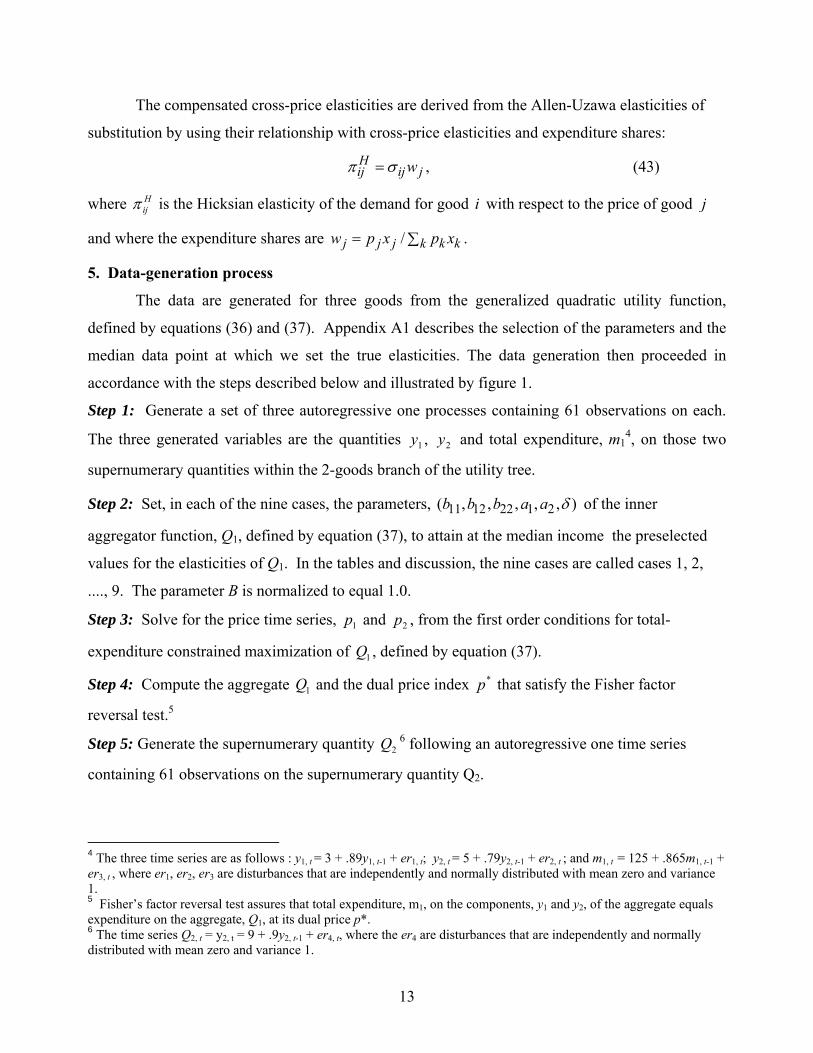
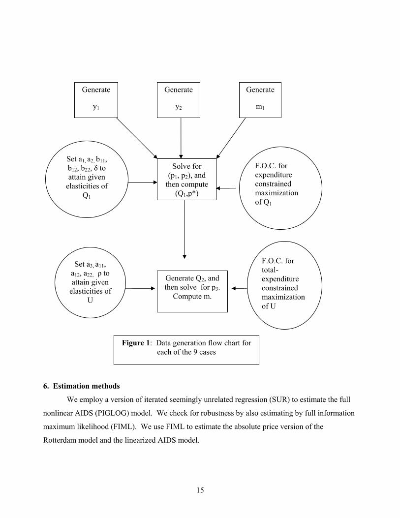
5. Data-generation process

The data are generated for three goods from the generalized quadratic utility function,

defined by equations (36) and (37). Appendix A1 describes the selection of the parameters and the

median data point at which we set the true elasticities. The data generation then proceeded in

accordance with the steps described below and illustrated by figure 1.

Step 1: Generate a set of three autoregressive one processes containing 61 observations on each.

The three generated variables are the quantities 1y , 2y and total expenditure, m14, on those two

supernumerary quantities within the 2-goods branch of the utility tree.

Step 2: Set, in each of the nine cases, the parameters, 11 12 22 1 2( , , , , , )b b b a a δ of the inner

aggregator function, Q1, defined by equation (37), to attain at the median income the preselected

values for the elasticities of Q1. In the tables and discussion, the nine cases are called cases 1, 2,

...., 9. The parameter B is normalized to equal 1.0.

Step 3: Solve for the price time series, 1p and 2p , from the first order conditions for total-

expenditure constrained maximization of 1Q , defined by equation (37).

Step 4: Compute the aggregate 1Q and the dual price index *p that satisfy the Fisher factor

reversal test.5

Step 5: Generate the supernumerary quantity 2Q 6 following an autoregressive one time series

containing 61 observations on the supernumerary quantity Q2.

4 The three time series are as follows : y1, t = 3 + .89y1, t-1 + er1, t; y2, t = 5 + .79y2, t-1 + er2, t ; and m1, t = 125 + .865m1, t-1 + er3, t , where er1, er2, er3 are disturbances that are independently and normally distributed with mean zero and variance 1. 5 Fisher’s factor reversal test assures that total expenditure, m1, on the components, y1 and y2, of the aggregate equals expenditure on the aggregate, Q1, at its dual price p*. 6 The time series Q2, t = y2, t = 9 + .9y2, t-1 + er4, t, where the er4 are disturbances that are independently and normally distributed with mean zero and variance 1.

14

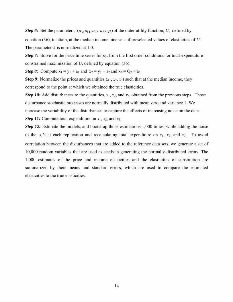
Step 6: Set the parameters, 3 11 12 22( , , , , )a a a a ρ of the outer utility function, U, defined by

equation (36), to attain, at the median income nine sets of preselected values of elasticities of U.

The parameter A is normalized at 1.0.

Step 7: Solve for the price time series for p3, from the first order conditions for total-expenditure

constrained maximization of U, defined by equation (36).

Step 8: Compute x1 = y1 + a1 and x2 = y2 + a2 and x3 = Q2 + a3.

Step 9: Normalize the prices and quantities (x1, x2, x3) such that at the median income, they

correspond to the point at which we obtained the true elasticities.

Step 10: Add disturbances to the quantities, x1, x2, and x3, obtained from the previous steps. Those

disturbance stochastic processes are normally distributed with mean zero and variance 1. We

increase the variability of the disturbances to capture the effects of increasing noise on the data.

Step 11: Compute total expenditure on x1, x2, and x3.

Step 12: Estimate the models, and bootstrap those estimations 1,000 times, while adding the noise

to the ix 's at each replication and recalculating total expenditure on x1, x2, and x3. To avoid

correlation between the disturbances that are added to the reference data sets, we generate a set of

10,000 random variables that are used as seeds in generating the normally distributed errors. The

1,000 estimates of the price and income elasticities and the elasticities of substitution are

summarized by their means and standard errors, which are used to compare the estimated

elasticities to the true elasticities.

15

6. Estimation methods

We employ a version of iterated seemingly unrelated regression (SUR) to estimate the full

nonlinear AIDS (PIGLOG) model. We check for robustness by also estimating by full information

maximum likelihood (FIML). We use FIML to estimate the absolute price version of the

Rotterdam model and the linearized AIDS model.

Set a1, a2, b11, b12, b22, δ to attain given

elasticities of Q1

Solve for (p1, p2), and

then compute (Q1,p*)

F.O.C. for expenditure constrained maximization of Q1

Generate

y1

Generate

y2

Generate

m1

Set a3, a11, a12, a22, ρ to attain given

elasticities of U

Generate Q2, and then solve for p3.

Compute m.

F.O.C. for total-expenditure constrained maximization of U

Figure 1: Data generation flow chart for each of the 9 cases

16

In estimating the nonlinear AIDS model, we first pick starting values for the parameters of

income’s price deflator (9). We substitute those starting values into the income deflator and

estimate the demand system (8), with the parameters of (9) treated as fixed. In the next step, the

resulting parameters for (8) are substituted into (9), and the iteration process continues until

convergence, defined to be when the differences between the parameter values in two successive

estimation are all less than or equal to 210− . This iterated SUR estimation procedure is analogous

to the one conventionally used with the relative price version of the Rotterdam model, which has a

similar source of nonlinearity from its use of the parameterized Frisch price index. As has been

shown with the relative price version of the Rotterdam model, this iterated SUR estimator produces

consistent estimates of all parameters and is considerably more convenient to use than FIML

estimation, when the source of nonlinearity is a price aggregator function embedded within the

model.7

The Rotterdam model represented by equation (3) will be estimated with the following

assumptions on the regressors and the disturbance vector. For each time 1, and , ,t t ntt DQ Dp Dp…

are nonstochastic. The disturbance vector, 1( , , )t t ntυ υ ′=υ … , has zero mean and time-independent

contemporaneous covariance matrix, [ ]ijω , which is a symmetric positive semi-definite nn×

matrix with rank 1−n and satisfies 1 0nijj ω= =∑ for each i . Also E 0][ =jtisεε for ts ≠ .

In addition, the theoretical symmetry of the Slutsky coefficient matrix ][ ijπ will be imposed

along with the linear homogeneity restrictions, ∑ ==

n

j ij10π and ∑=

=n

i i11μ .

7. Performance of Different Price Approximations

It is common in the literature to linearize the AIDS model by using Stone’s nonparametric

statistical index, (17), to approximate income’s parameterized price-deflator. But that

approximation has shortcomings. Pashardes (1993) has shown that errors resulting from that

approximation can be seen as an omitted variable. The resulting estimates of the parameters of the

demand functions may thereby be biased. In addition, Moschini(1995) pointed out that Stone's

7Although this estimator is consistent, it is not asymptotically efficient. Barnett’s (1976) result on the asymptotic equivalence of FIML with iterated Aitken are not applicable here, since his proof assumes no overlap between the parameters on each side of the iteration. The purpose of this iterated SUR estimator with the relative price version of the Rotterdam model has been to capture the consistency acquired from joint estimation, while minimizing transmission of errors in estimation of the price aggregator function’s parameters to the estimators of the demand function’s parameters. We explore that potential contamination by also using FIML for comparison.

17

index failed to satisfy the "commensurability" property, in the sense that the growth rate of the

price index is not invariant to the unit of measurement of prices. Moschini suggests three

alternative indexes: the Törnqvist index and two normalized forms of the Stone index.8 In this

section, we will investigate whether these alternative price approximations perform better or worse

than the exact price index, when preferences are generated from Barnett’s (1977) WS-branch

model.

7.1 The Törnqvist price index

Diewert (1976) showed that the Törnqvist index is exact for the translog unit cost function,9

*0 0

1 1 1

1log ( ) log log log2

N N Nk k kj k j

k k jc p p p pα α γ

= = == + +∑ ∑ ∑ , (44)

where jiij γγ = , ∑ ==

N

k i11α , and 0

1=∑ =

N

k kjα for Nk ,,2,1 …= . Therefore, the Törnqvist price

index is a superlative price index, in the sense defined by Diewert (1976). The fixed-base

Törnqvist price index (often called the Divisia price index in discrete time, when chained) is

defined by:

00

1log ( ) log2

jtTt jt j

j j

pP w w

p= +∑ . (45)

Hence,

0 0

1 1

log 1 1 1log loglog 2 log 2 2

T n nt ktjt kt k j

k kjt jt

P ww p p wp p= =

⎡ ⎤∂ ∂= + − +∑ ∑⎢ ⎥

∂ ∂⎢ ⎥⎣ ⎦

001

log1 ( ) log2 log

n kt ktjt j kt

k jtk

p ww w wpp=

⎡ ⎤⎛ ⎞ ∂⎢ ⎥= + + ⎜ ⎟∑ ⎜ ⎟ ∂⎢ ⎥⎝ ⎠⎣ ⎦

8We follow Moschini in using fixed base indexes, since chained indexes would diverge further from the underlying theory on which the AIDS model was derived. Nevertheless, we plan future research on the robustness of our conclusions to the use of chained indexes. 9A price index P is exact for a neoclassical aggregator function f having unit cost function dual c, if P(p1,p2,s1,s2) = c(p2)/c(p1), where (x1,x2) is the solution to the maximization of the aggregator function f subject to total cost constraint.

18

001

1 ( ) log ( )2

n ktjt j kt kj kj

k k

pw w wp

ε δ=

⎡ ⎤⎛ ⎞⎢ ⎥= + + +⎜ ⎟∑ ⎜ ⎟⎢ ⎥⎝ ⎠⎣ ⎦

, (46)

where εkj is the Marshallian cross price elasticity, (18), and δkj is the Kronecker delta (14).

Substituting (46) into (21), the uncompensated cross-price elasticity of demand for good i with

respect to the price of good j is

001

1 ( ) log ( )2

nij i ktij ij jt j kt kj kj

ki i k

pw w ww w p

γ βε δ ε δ

=

⎡ ⎤⎛ ⎞⎛ ⎞ ⎢ ⎥= − + − + + +⎜ ⎟∑⎜ ⎟ ⎜ ⎟⎝ ⎠ ⎢ ⎥⎝ ⎠⎣ ⎦. (47)

Let E be the matrix of price elasticities. Equation (47) can be written in matrix notation as

*1* ( )2⎡ ⎤′= − +⎢ ⎥⎣ ⎦

E A kc E I , (48)

where [ ]ijε=E and ** ija⎡ ⎤= ⎣ ⎦A are nn× matrices, with E the matrix of elasticities, and

0* ( )

/2

i jt jij ij ij i

i

w wa w

wβ

δ γ+

= − + − , * * *1 2* ( , , , )nc c c ′=c … with *

0log jtj j

j

pc w

p

⎛ ⎞⎜ ⎟=⎜ ⎟⎝ ⎠

, and

1 2( , , , )nk k k ′=K … with /i i ik wβ= . Solving (48) for E yields

( )1

*1 *2

−⎛ ⎞′= + + −⎜ ⎟⎝ ⎠

E I kc A I I . (49)

The derivation of the income elasticities is analogous and uses

01

log 1 loglog 2 log

T n kt k

k k

p wPm mp=

⎛ ⎞ ∂∂= ⎜ ⎟∑ ⎜ ⎟∂ ∂⎝ ⎠

01 log ( 1).2

n ktkt k

k k

pwp

η⎛ ⎞

= −⎜ ⎟∑ ⎜ ⎟⎝ ⎠

(50)

Substituting (50) into the general expression for income elasticity as a function of the derivative of

the log-change of the price index with respect to income, we obtain

01 11 log ( 1)

2

n kti i kt k

ki k

pww p

η β η⎡ ⎤⎛ ⎞⎢ ⎥= + − −⎜ ⎟∑ ⎜ ⎟⎢ ⎥⎝ ⎠⎣ ⎦

(51)

This expression can be written in matrix notation as follows:

19

*12

′= −n k kc n , (52)

where n is as defined in (30). Hence n is an n dimensional vector with elements 1−= iin η . After

some manipulation, the income elasticities are obtained. In matrix notation, after solving for n, we

get

1

*12

−⎛ ⎞′= +⎜ ⎟⎝ ⎠

n I kc k (53).

7.2 A first modified Stone's index (Paasche-like index )

As shown by Moschini (1995), Stone's index can be modified to be invariant to the unit of

measurement. We call the modified index the quasi-Paasche index, since it uses current period

expenditure weights. The resulting price index in logarithms is

0log logP ktt kt

k k

pP wp

= ∑ . (54)

Using this price index, the price elasticities will be slightly different from those generated using

Stone's index. Indeed, equation (22) becomes, after some manipulations,

0log logloglog log

Pt kt kt

jt ktkjt jtk

P p ww wp pp

∂ ∂= +∑

∂ ∂ (55)

Then the Marshallian price elasticities become analogous to (39), but with kplog replaced by

0log / logkt kp p . We substitute (55) into (21) to acquire the price elasticities. In matrix notation,

the matrix of price elasticities is given by

( ) ( )1

* ,−

′= + + −E I kc A I I (56)

where the variables are as defined in section 3.3.

We now compute the income derivatives of the price index:

01

log loglog log

P nt kt kt

kt tk

P p wm mp=

⎛ ⎞∂ ∂= ⎜ ⎟∑ ⎜ ⎟∂ ∂⎝ ⎠

0log ( 1)n kt

kt kk k

pwp

η⎛ ⎞

= −⎜ ⎟∑ ⎜ ⎟⎝ ⎠

. (57)

20

In matrix notation, we have the following result, which is the analogous to (52):

*′= −n k kc n , (58)

where the variables are as previously defined. Solving for n, we get

( ) 1*

−′= +n I kc k . (59)

7.3 A second modified Stone's index (Laspeyres-like index)

Moschini (1995) also proposed a Laspeyres-like modification, PL, of Stone’s index. This

modification is the analog to the Laspeyres index in logarithms, with weights computed from base

period expenditures. The index is

00log log jtL

t jj j

pP w

p= ∑ . (60)

Then it follows immediately that

0loglog

Lt

jjt

P wp

∂=

∂. (61)

The price elasticity of good i with respect to the price of good j is given by

0ij iij ij j

it itw

w wγ β

ε δ= − + − . (62)

The income elasticity of good i becomes

1 ii

itwβ

η = + , (63)

which is the same as (15) for the full nonlinear AIDS model. The formulas for the elasticities in

this case are close to those of the full nonlinear AIDS, but not identical for the price elasticities.

8. Estimation Results

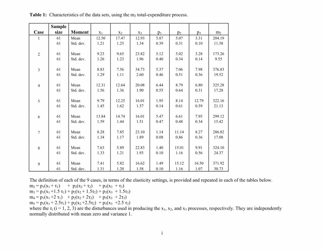
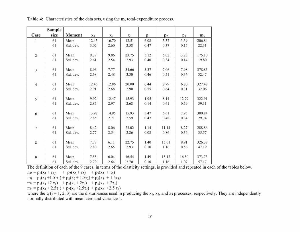
Tables 1-4 summarize the stochastic properties of the generated data. We report the mean

and standard deviations of the quantities of three commodities, 21, xx and 3x , of their respective

prices, 21, pp and 3p , and of the total-expenditure processes. Total expenditure appears more

volatile than prices and quantities, as is consistent with real world data. We use four specifications

21

of the total-expenditure processes, m2, m3, m4, and m5.10 See the footnote to table 1 for the

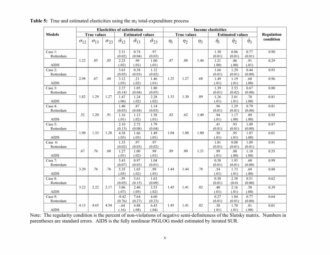
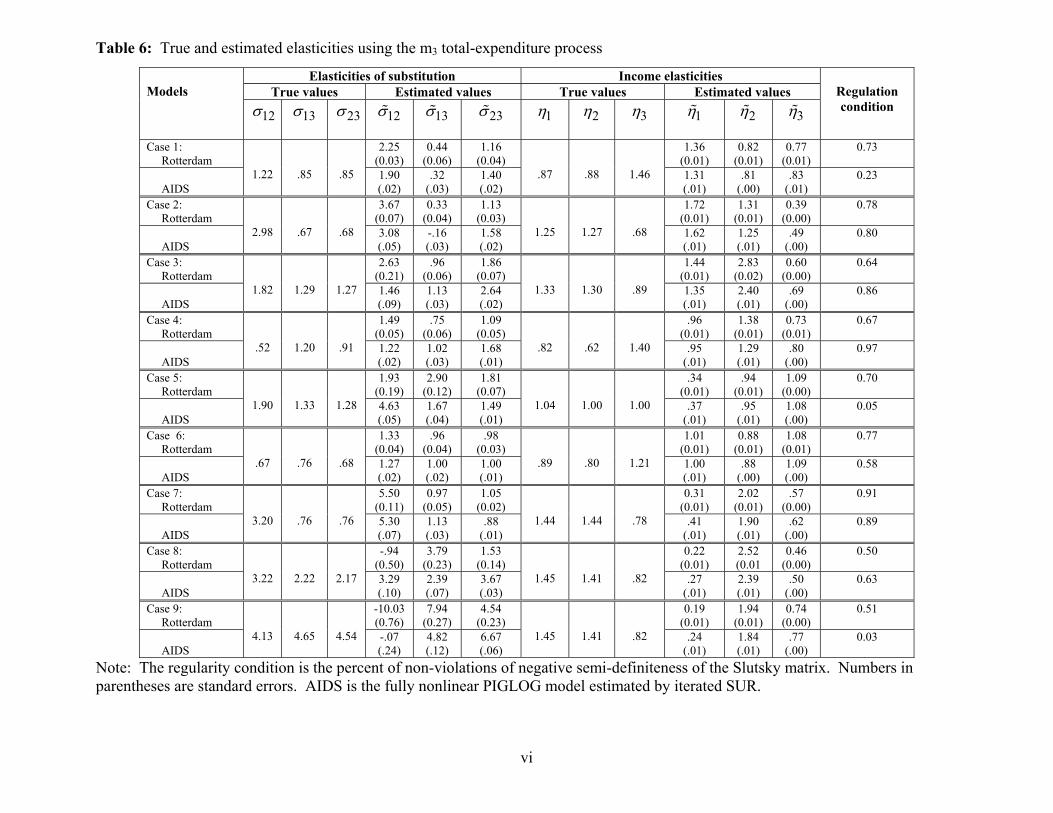
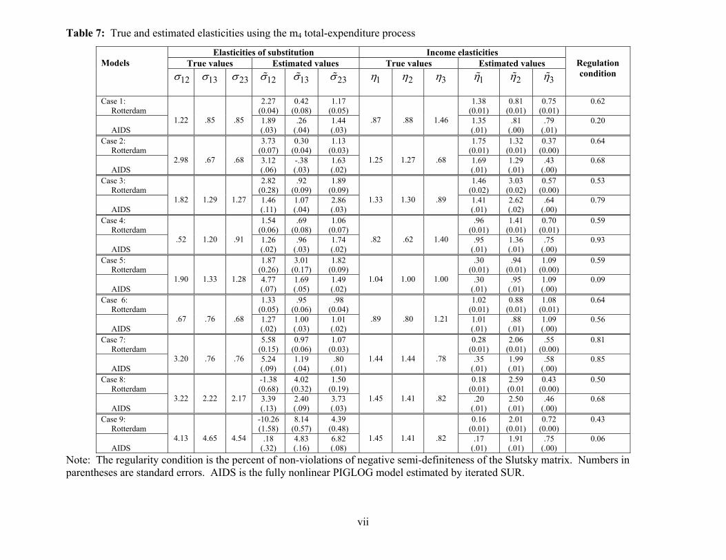
definition of the four specifications.11 Tables 5 - 8 provide comparisons of performance of the

Rotterdam model with the full nonlinear AIDS (PIGLOG) model.

Looking at the estimates of income elasticities, we observe that the two models yield similar

results. Quantitatively, when the AIDS overestimates or underestimates the income elasticities, the

Rotterdam also does. Qualitatively though, the results are similar.

The two models depart from one another in their performance in recovering the true

elasticities of substitution. In cases 1, 2, and 7, where the true elasticity of substitution among

goods in the inner aggregator function, 12σ , is high and low among pairs of goods in different

aggregator functions, 13σ and 23σ , both models produce higher estimates of 12σ , with the AIDS

estimates lower than the Rotterdam estimates. The estimates of 13σ from the Rotterdam are slightly

closer to the true values and the ranking of the two models in estimating 23σ favors the Rotterdam

in two out of three cases. Qualitatively though, the Rotterdam dominates. In fact the AIDS

misclassifies goods 1 and 3 as complements, when they are substitutes by construction.12

When all elasticities of substitution, 12σ , 13σ , 23σ , are moderately high (cases 3 and 5),

both models perform relatively well in estimating all three of the elasticities of substitution. This

finding that the Rotterdam model produces satisfactory estimates of elasticities of substitution in

this case corroborates Barnett and Choi (1989), who acquired similarly positive results for the

Rotterdam model with data produced from homothetic preferences.

The same observations apply when the elasticities of substitution are all low, as in

case 6. Quantitatively, both models overestimate the elasticities, but the Rotterdam estimates of 13σ

and 23σ are always slightly smaller than the AIDS estimates. When, as in case 4, the elasticity

within the aggregator function ( 12σ ) is low and higher between goods in different aggregator

functions, both models overestimate the lower elasticities ( 12σ , 23σ ), and underestimate the higher

elasticity of substitution.

10Recall that m1 has already been defined to be expenditure on only two of the three supernumerary quantities. 11In the specifications of the total expenditure processes, m2, m3, m4, and m5, the errors in total expenditure are a combination of the errors in the quantities. 12This tendency to classify two goods as complements, when they are actually substitutes, has been found previously for the translog model by Guilkey and Lovell (1980) and Guilkey, Lovell and Sickles (1983).

22

But in cases 8 and 9, all of the true elasticities of substitution are generally unusually high.

In such cases, indifference curves are almost linear. In those cases, the two models performed

poorly in estimating the higher elasticity of substitution between goods within the inner aggregator

function, 12σ (case 9). The precision of that estimated elasticity is very low, with the standard

deviation being about three times greater than the estimated value of the elasticity. The AIDS

accommodated the high elasticities better than the Rotterdam, since AIDS performed well in case 8

for the four specifications of the disturbances.

In case 9, that result on low precision was found with all of our specifications of the total

expenditure process, as seen in tables 5 through 8. Surprisingly, that low precision does not appear

for the estimated substitutability between pairs of goods in different aggregator functions. For those

pairs of good in cases 8 and 9, the two models yield positive, very high elasticities of substitution

with small standard deviations. This high precision relative to that of the estimated elasticity

between goods 1 and 2 is an unexpected finding.

A consistent pattern appears in the standard errors of the two models and in the regularity

condition column of the tables. The AIDS produces smaller standard errors in all 9 cases and with

all specifications of total-expenditure. The percentage of violations of the Slutsky matrix’s negative

semi-definiteness does not appear to be a factor in the relative performance of the two models.

However, for high percentages of violations, the AIDS would perform qualitatively poorly (cases 1,

5, 9).

The theoretical properties of the demand function are known only when the regularity

conditions are satisfied, since the duality theory on which the models’ derivations are based require

regularity. Hence the violations of negative semi-definiteness can be a source of the relatively poor

performance of the AIDS model in estimating elasticities.13

The differences in the performances between the Rotterdam and the nonlinear AIDS models

are not the result of the different estimation methods, namely the Iterated SUR (ITSUR) with the

nonlinear AIDS model and FIML for the Rotterdam model and linearized AIDS model. For

comparison, we also estimated the nonlinear AIDS with FIML. No significant differences were

found between nonlinear AIDS with ITSUR and with FIML14.

13Regarding the nature of this problem with other models, see Caves and Christensen (1980), Barnett and Lee (1985), and Barnett et al. (1985). 14The results of that comparison can be obtained from the authors upon request.

23

Tables 9a-9i contain the results of our estimations of the Linear Approximated AIDS (LA-

AIDS), when different price indices are used to produce the linearization. In the literature, the most

popular LA-AIDS uses Stone's index, which produced the original AIDS model of Deaton and

Muellbauer. We also estimated linear AIDS models using three other price indices: the Törnqvist

index and the two price-normalized modified-Stone indexes, motivated by the Paasche and

Laspeyres indexes. It is immediately evident that the linear approximations yield results very

different from those obtained from the nonlinear AIDS model in tables 5-8.

The results from the four linearized models are very similar quantitatively and qualitatively.

But the sign problems that the nonlinear AIDS models were displaying sometimes became worse.

The results in tables 9a-9i show that the linearly approximated AIDS models perform significantly

differently from the PIGLOG model they are designed to approximate.

9. Conclusion

Among the many demand specifications in the literature, the Rotterdam model and the

Almost Ideal Demand System (AIDS) have particularly long histories, have been highly developed,

and are often applied in consumer demand systems modeling. Using Monte Carlo techniques, we

seek to determine which model performs better in terms of its ability to recover the true elasticities

of demand. Three findings follow from this paper:

[1] Both the Rotterdam and the PIGLOG (fully nonlinear AIDS) models perform well, when

substitution among goods is low. The higher the level of aggregation, the lower the

elasticity of substitution among aggregates. Therefore when modeling consumer demand

at the aggregate level, both models may yield correct estimates of the elasticities of

substitution.

[2] When the elasticities of substitutions among goods is moderately high, both models

perform well.

[3] When substitution among all goods is very high, the nonlinear PIGLOG perform better

than the Rotterdam.

[4] The Rotterdam model appears better at recovering the true elasticities, when we

implement exact aggregation within weakly separable branches of a utility tree. When

attempting to build consistent aggregates, the Rotterdam appears to perform better.

Within weakly separable branches of the utility tree, the nonlinear PIGLOG model may

24

classify substitutes as complements or overestimate the elasticities of substitution among

goods.

We derive the formulas for the linearized AIDS model’s elasticities, when the Törnqvist

price index or either of two modified Stone indexes are used to linearize the model. We find that

these three indices, along with Stone’s widely used price index, do not yield satisfactory results.

The use of those linearizations exacerbates misclassification of goods as complements and leads to

estimated elasticities different from those of the full nonlinear PIGLOG model, which the

linearized AIDS models are designed to approximate.

These findings are robust in the sense that they do not change, whether we estimate the

PIGLOG, AIDS, or Rotterdam models using ITSUR or FIML estimation.

25

10. References Allen RGD. 1938. Mathematical analysis for economists. Macmillan: London.

Allen RGD, Hicks JR. 1934. A reconsideration of the theory of value, II. Economica 1(2): 196-219.

Alston JM, Chalfant A. 1993. The silence of the Lamdas: a test for the Almost Ideal and Rotterdam models.

American Journal of Agricultural Economics 75: 304-14.

Alston JM, Foster KA, Green R. 1994. Estimating elasticities with the linear approximate ideal demand system:

some Monte Carlo results. Review of Economics and Statistics 76:351-56.

Arrow KJ, Chenery HB, Minhas BS, Solow RM. 1961. Capital-labor substitution and economic efficiency. Review

of Economics and Statistics 43:225-50.

Banks J, Blundell R, Lewbel A. 1997. Quadratic Engel curves and consumer demand. Review of Economics and

Statistics 79:527-39.

Barnett WA. 1976. Maximum likelihood and iterated Aitken estimation of non-linear systems of equations.

Journal of the American Statistical Association 71:354-360.

Barnett WA. 1977. Recursive subaggregation and a generalized hypocycloidal demand model. Econometrica 45:

1117-1136.

Barnett WA. 1979. Theoretical foundations of the Rotterdam model. Review of Economic Studies 46: 109-30.

Barnett WA. 1983. New indices of money supply and the flexible Laurent demand system. Journal of Business

and Economic Statistics 1: 7-23.

Barnett WA, Jonas A. 1983. The Muntz-Szatz demand system: an application of a globally well-behaved series

expansion. Economic Letters 11(4): 337-42.

Barnett WA. 1985. The Minflex Laurent Translog flexible functional form. Journal of Econometrics 30: 33-44.

Barnett WA., Lee WY. 1985. The global properties of the Minflex Laurent, Generalized Leontief and Translog

flexible functional forms. Econometrica 53: 1421-1437.

26

Barnett WA, Lee WY, Wolfe MD. 1985. The three- dimensional global properties of the Minflex Laurent,

Generalized Leontief, and Translog flexible functional forms. Journal of Econometrics 30: 3-31.

Barnett WA., Lee WY, Wolfe MD. 1987. The global properties of the two Minflex Laurent flexible functional

forms. Journal of Econometrics 36: 281-98.

Barnett WA, Choi S. 1989. A Monte Carlo study of tests of blockwise weak separability. Journal of Business and

Economic Statistics 7: 363-377.

Barnett WA, Yue P. 1998. Semiparametric estimation of the Asymptotically Ideal Model: the AIM demand

system. In Nonparametric and Robust Inference, Advances in Econometrics 7, Rhodes G, Formby T(eds). JAI

Press: Greenwich, CT; 229-52.

Barten AP. 1964. Consumer demand functions under conditions of almost additive preferences. Econometrica 32:

1-38.

Barten AP. 1968. Estimating demand equations. Econometrica Vol. 36(2): 213-51.

Barten AP. 1977. The systems of consumer demand functions approach: A Review. Econometrica 45: 23-51.

Berndt ER, Darrough MN, Diewert WE. 1977. Flexible functional forms and expenditure distribution: an

application to Canadian consumer demand functions. International Economic Review. 18: 651-75.

Blackorby C, Russell RR. 1981. The Morishima elasticity of substitution: symmetry, constancy, separability, and

its relationship to the Hicks and Allen elasticities. Review of Economic Studies 48: 147-58.

Blackorby C, Russell RR. 1989. Will the real elasticity of substitution please stand up? (A comparison of the

Allen/Uzawa and Morishima elasticities). American Economic Review 79: 882-888.

Caves DW, Christensen LR. 1980. Global properties of flexible functional forms. American Economic Review 70:

422-32.

Christensen LR, Jorgenson DW, Lau LJ. 1975. Transcendental logarithmic utility functions. American Economic

Review 65: 367-83.

Cooper RJ, McLaren KR. 1996. A system of demand equations satisfying effectively global regularity conditions.

Review of Economics and Statistics.

27

Deaton A, Muellbauer J. 1980a. An Almost Ideal Demand System. American Economic Review 70: 312-26.

Deaton A, Muellbauer J. 1980b. Economics and consumer behavior. Cambridge University Press.

Denny M. 1974. The relationship between functional forms for production systems. Canadian Journal of

Economics 7: 21-31.

Diewert WE. 1971. An Application of the Shephard duality theorem: a Generalized Leontief production function.

Journal of Political Economy 79: 461-507.

Diewert WE. 1976. Essays in index number theory. North Holland: Amsterdam.

Fisher D, Fleissig AR, Serletis A. 2001. An empirical comparison of flexible demand system functional forms.

Journal of Applied Econometrics 16: 59-80.

Gallant AR. 1981. On the bias in flexible functional forms and an essentially unbiased form: The Fourier flexible

form. Journal of Econometrics 15: 211-45.

Green, R. and JM Alston. 1990. Elasticities in AIDS Models. American Journal of Agricultural Economics. 72:

442-445.

Guilkey DK, Lovell CAK, Sickles RC. 1980. On the flexibility of the translog approximation. International

Economic Review. 21:137-147.

Guilkey DK, Lovell CAK. 1983. A comparison of the performance of three flexible functional forms. International

Economic Review. 24: 591-616.

Hicks JR. 1932. Theory of wages. Macmillan: London.

Kadiyala KR. 1972. Production functions and elasticity of substitution. Southern Economic Journal 38: 281-284.

Morishima M. 1967. A few suggestions on the theory of elasticity. Keizai Hyoron (Economic Review) 16: 149-

150.

Moschini G. 1995. Units of measurement and the Stone index in demand system estimation, American Journal of

Agricultural Economics 77: 63-68.

28

Pashardes A. 1993. Bias in the estimation of the Almost Ideal Demand System with the Stone index

approximation. Economic Journal 103: 908-915.

Theil H. 1965. The information approach to demand analysis. Econometrica 33: 67-87.

Theil H. 1975a. Theory and measurement of consumer demand. Volume 1 . Amsterdam: North-Holland.

Theil H. 1975b. Theory and measurement of consumer demand. Volume 2. Amsterdam: North-Holland.

Uzawa H. 1962. Production functions with constant elasticity of substitution. Review of Economic Studies 30:

291-99.

29

Appendix A1: Selection of the values of the generating model’s utility-function parameters and of the median vector of

variables, (prices, quantities and expenditures).

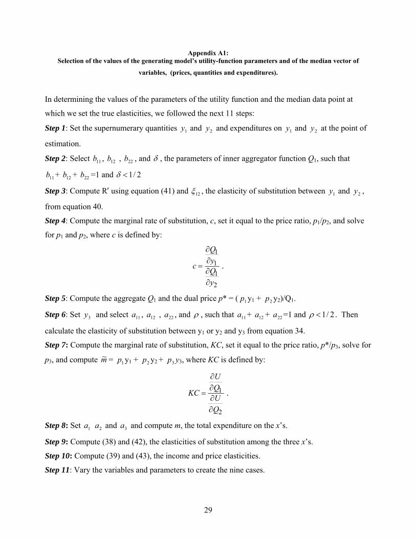
In determining the values of the parameters of the utility function and the median data point at

which we set the true elasticities, we followed the next 11 steps:

Step 1: Set the supernumerary quantities 1y and 2y and expenditures on 1y and 2y at the point of

estimation.

Step 2: Select 11b , 12b , 22b , and δ , the parameters of inner aggregator function Q1, such that

11b + 12b + 22b =1 and 1/ 2δ <

Step 3: Compute R’ using equation (41) and 12ξ , the elasticity of substitution between 1y and 2y ,

from equation 40.

Step 4: Compute the marginal rate of substitution, c, set it equal to the price ratio, p1/p2, and solve

for p1 and p2, where c is defined by:

1

11

2

Qyc Qy

∂∂

=∂∂

.

Step 5: Compute the aggregate Q1 and the dual price p* = ( 1p y1 + 2p y2)/Q1.

Step 6: Set 3y and select 11a , 12a , 22a , and ρ , such that 11a + 12a + 22a =1 and 1/ 2ρ < . Then

calculate the elasticity of substitution between y1 or y2 and y3 from equation 34.

Step 7: Compute the marginal rate of substitution, KC, set it equal to the price ratio, p*/p3, solve for

p3, and compute m~ = 1p y1 + 2p y2 + 3p y3, where KC is defined by:

1

2

UQKC UQ

∂∂

=∂∂

.

Step 8: Set 1a 2a and 3a and compute m, the total expenditure on the x’s.

Step 9: Compute (38) and (42), the elasticities of substitution among the three x’s.

Step 10: Compute (39) and (43), the income and price elasticities.

Step 11: Vary the variables and parameters to create the nine cases.

i

Table 1: Characteristics of the data sets, using the m2 total-expenditure process.

Case Sample

size Moment x1 x2 x3 p1 p2 p3 m2 61 Mean 12.50 17.47 12.93 5.87 5.07 3.31 204.19 1

61 Std. dev. 1.21 1.25 1.34 0.39 0.31 0.10 11.58

61 Mean 9.23 9.65 23.82 5.12 5.02 3.28 173.26 2 61 Std. dev. 1.26 1.23 1.96 0.40 0.34 0.14 9.55

61 Mean 8.83 7.56 34.73 5.37 7.06 7.98 376.83

3 61 Std. dev. 1.29 1.11 2.60 0.46 0.51 0.36 19.52

61 Mean 12.31 12.64 20.08 6.44 8.79 6.80 325.28

4 61 Std. dev. 1.56 1.36 1.90 0.55 0.64 0.31 17.28

61 Mean 9.79 12.25 16.01 1.95 8.14 12.79 322.16

5 61 Std. dev. 1.45 1.62 1.57 0.14 0.61 0.59 21.13

61 Mean 13.84 14.74 16.01 5.47 6.61 7.95 299.12

6 61 Std. dev. 1.59 1.44 1.51 0.47 0.48 0.34 15.42

61 Mean 8.28 7.85 23.10 1.14 11.14 8.27 286.82

7 61 Std. dev. 1.34 1.17 1.89 0.08 0.86 0.36 17.08

61 Mean 7.63 5.89 22.83 1.40 15.01 9.91 324.10

8 61 Std. dev. 1.33 1.21 1.93 0.10 1.16 0.56 24.37

61 Mean 7.41 5.82 16.62 1.49 15.12 16.50 371.92

9 61 Std. dev. 1.31 1.20 1.58 0.10 1.16 1.07 30.73

The definition of each of the 9 cases, in terms of the elasticity settings, is provided and repeated in each of the tables below. m2 = p1(x1 + τ1) + p2(x2 + τ2) + p3(x3 + τ3) m3 = p1(x1 +1.5 τ1) + p2(x2 + 1.5τ2) + p3(x3 + 1.5τ3) m4 = p1(x1 +2 τ1) + p2(x2 + 2τ2) + p3(x3 + 2τ3) m5 = p1(x1 + 2.5τ1) + p2(x2 +2.5τ2) + p3(x3 +2.5 τ3) where the τi (i = 1, 2, 3) are the disturbances used in producing the x1, x2, and x3 processes, respectively. They are independently normally distributed with mean zero and variance 1.

ii


Case Sample


61 Std. dev. 2.05 1.76 1.75 0.47 0.37 0.15 14.22

61 Mean 9.28 9.72 23.80 5.12 5.02 3.28 173.88 2 61 Std. dev. 1.65 1.63 2.23 0.40 0.34 0.14 12.64

61 Mean 8.87 7.63 34.71 5.37 7.06 7.98 377.50

3 61 Std. dev. 1.70 1.54 2.77 0.46 0.51 0.36 23.15

61 Mean 12.36 12.72 20.05 6.44 8.79 6.80 326.01

4 61 Std. dev. 1.95 1.77 2.18 0.55 0.64 0.31 21.58

61 Mean 9.83 12.33 15.98 1.95 8.14 12.79 322.41

5 61 Std. dev. 1.87 2.04 1.90 0.14 0.61 0.59 26.48

61 Mean 13.88 14.81 15.98 5.47 6.61 7.95 299.69

6 61 Std. dev. 1.94 1.83 1.82 0.47 0.48 0.34 19.69

61 Mean 8.33 7.92 23.07 1.14 11.14 8.27 287.50

7 61 Std. dev. 1.77 1.60 2.16 0.08 0.86 0.36 22.79

61 Mean 7.68 5.96 22.80 1.40 15.01 9.91 324.86

8 61 Std. dev. 1.78 1.68 2.21 0.10 1.16 0.56 31.18

61 Mean 7.46 5.89 16.59 1.49 15.12 16.50 372.53

9 61 Std. dev. 1.77 1.67 1.91 0.10 1.16 1.07 38.48


iii


Case Sample


61 Std. dev. 2.52 2.16 2.15 0.47 0.37 0.15 18.17

61 Mean 9.32 9.79 23.77 5.12 5.02 3.28 174.49 2 61 Std. dev. 2.11 2.07 2.56 0.40 0.34 0.14 16.13

61 Mean 8.92 7.70 34.68 5.37 7.06 7.98 378.18

3 61 Std. dev. 2.17 2.01 3.01 0.46 0.51 0.36 27.58

61 Mean 12.40 12.79 20.03 6.44 8.79 6.80 326.75

4 61 Std. dev. 2.42 2.22 2.52 0.55 0.64 0.31 26.63

61 Mean 9.88 12.40 15.95 1.95 8.14 12.79 322.66

5 61 Std. dev. 2.34 2.50 2.27 0.14 0.61 0.59 32.59

61 Mean 13.93 14.88 15.95 5.47 6.61 7.95 300.26

6 61 Std. dev. 2.37 2.26 2.18 0.47 0.48 0.34 24.57

61 Mean 8.37 7.99 23.05 1.14 11.14 8.27 288.18

7 61 Std. dev. 2.26 2.06 2.49 0.08 0.86 0.36 29.05

61 Mean 7.72 6.03 22.78 1.40 15.01 9.91 325.62

8 61 Std. dev. 2.27 2.16 2.55 0.10 1.16 0.56 38.94

61 Mean 7.51 5.96 16.56 1.49 15.12 16.50 373.13

9 61 Std. dev. 2.27 2.15 2.29 0.10 1.16 1.07 47.49


iv


Case Sample


61 Std. dev. 3.02 2.60 2.58 0.47 0.37 0.15 22.31

61 Mean 9.37 9.86 23.75 5.12 5.02 3.28 175.10 2 61 Std. dev. 2.61 2.54 2.93 0.40 0.34 0.14 19.80

61 Mean 8.96 7.77 34.66 5.37 7.06 7.98 378.85

3 61 Std. dev. 2.68 2.48 3.30 0.46 0.51 0.36 32.47

61 Mean 12.45 12.86 20.00 6.44 8.79 6.80 327.48

4 61 Std. dev. 2.91 2.68 2.90 0.55 0.64 0.31 32.06

61 Mean 9.92 12.47 15.93 1.95 8.14 12.79 322.91

5 61 Std. dev. 2.85 2.97 2.68 0.14 0.61 0.59 39.11

61 Mean 13.97 14.95 15.93 5.47 6.61 7.95 300.84

6 61 Std. dev. 2.85 2.71 2.59 0.47 0.48 0.34 29.74

61 Mean 8.42 8.06 23.02 1.14 11.14 8.27 288.86

7 61 Std. dev. 2.77 2.54 2.86 0.08 0.86 0.36 35.57

61 Mean 7.77 6.11 22.75 1.40 15.01 9.91 326.38

8 61 Std. dev. 2.80 2.65 2.93 0.10 1.16 0.56 47.19

61 Mean 7.55 6.04 16.54 1.49 15.12 16.50 373.73

9 61 Std. dev. 2.79 2.64 2.70 0.10 1.16 1.07 57.17


v

Table 5: True and estimated elasticities using the m2 total-expenditure process

Elasticities of substitution Income elasticities True values Estimated values True values Estimated values

Models

12σ

13σ 23σ

12σ 13σ 23σ 1η 2η 3η 1η 2η 3η

Regulation condition

Case 1: Rotterdam

2.31 (0.02)

0.74 (0.04)

.97 (0.03)

1.30 (0.01)

0.86 (0.01)

0.77 (0.01)

0.90

AIDS

1.22

.85

.85 2.25 (.02)

.99 (.01)

1.00 (.01)

.87

.88

1.46 1.21 (.00)

.86 (.00)

.91 (.01)

0.29

Case 2: Rotterdam

3.63 (0.05)

0.38 (0.03)

1.12 (0.02)

1.66 (0.01)

1.29 (0.01)

0.44 (0.00)

0.93

AIDS

2.98

.67

.68 3.12 (.03)

.21 (.02)

1.46 (.01)

1.25

1.27

.68 1.49 (.01)

1.19 (.01)

.60 (.00)

0.96

Case 3: Rotterdam

2.37 (0.14)

1.05 (0.04)

1.80 (0.05)

1.39 (0.01)

2.53 (0.02)

0.67 (0.00)

0.80

AIDS

1.82

1.29

1.27 1.47 (.06)

1.24 (.02)

2.28 (.02)

1.33

1.30

.89 1.26 (.01)

2.01 (.01)

.78 (.00)

0.81

Case 4: Rotterdam

1.40 (0.03)

.87 (0.04)

1.14 (0.03)

.96 (0.01)

1.29 (0.01)

0.79 (0.00)

0.81

AIDS

.52

1.20

.91 1.16 (.01)

1.13 (.02)

1.58 (.01)

.82

.62

1.40 .94 (.01)

1.17 (.00)

.89 (.00)

0.95

Case 5: Rotterdam

2.10 (0.13)

2.72 (0.08)

1.79 (0.04)

.41 (0.01)

.93 (0.01)

1.09 (0.00)

0.87

AIDS

1.90

1.33

1.28 4.38 (.03)

1.66 (.03)

1.49 (.01)

1.04

1.00

1.00 .50 (.01)

.95 (.01)

1.07 (.00)

0.01

Case 6: Rotterdam

1.33 (0.02)

.97 (0.03)

.97 (0.02)

1.01 (0.01)

0.88 (0.01)

1.09 (0.01)

0.91

AIDS

.67

.76

.68 1.27 (.01)

1.00 (.02)

.99 (.01)

.89

.80

1.21 .99 (.01)

.88 (.00)

1.10 (.00)

0.55

Case 7: Rotterdam

5.43 (0.07)

0.97 (0.03)

1.04 (0.01)

0.38 (0.01)

1.93 (0.01)

.60 (0.00)

0.99

AIDS

3.20

.76

.76 5.35 (.05)

1.03 (.02)

.99 (.01)

1.44

1.44

.78 .54 (.01)

1.73 (.01)

.69 (.00)

0.88

Case 8: Rotterdam

-.59 (0.05)

3.61 (0.15)

1.63 (0.09)

0.30 (0.01)

2.38 (0.01

0.51 (0.00)

0.62

AIDS

3.22

2.22

2.17 3.06 (.07)

2.40 (.05)

3.53 (.02)

1.45

1.41

.82 .40 (.01)

2.16 (.01)

.58 (.00)

0.39

Case 9: Rotterdam

-9.42 (0.76)

7.64 (0.27)

4.60 (0.23)

0.27 (0.01)

1.84 (0.01)

0.77 (0.00)

0.64

AIDS

4.13

4.65

4.54 -.64 (.16)

4.88 (.08)

6.43 (.04)

1.45

1.41

.82 .38 (.01)

1.70 (.01)

.81 (.00)

0.01

Note: The regularity condition is the percent of non-violations of negative semi-definiteness of the Slutsky matrix. Numbers in parentheses are standard errors. AIDS is the fully nonlinear PIGLOG model estimated by iterated SUR.

vi



Models

12σ

13σ 23σ

12σ 13σ 23σ 1η 2η 3η 1η 2η 3η


Case 1: Rotterdam

2.25 (0.03)

0.44 (0.06)

1.16 (0.04)

1.36 (0.01)

0.82 (0.01)

0.77 (0.01)

0.73

AIDS

1.22

.85

.85 1.90 (.02)

.32 (.03)

1.40 (.02)

.87

.88

1.46 1.31 (.01)

.81 (.00)

.83 (.01)

0.23

Case 2: Rotterdam

3.67 (0.07)

0.33 (0.04)

1.13 (0.03)

1.72 (0.01)

1.31 (0.01)

0.39 (0.00)

0.78

AIDS

2.98

.67

.68 3.08 (.05)

-.16 (.03)

1.58 (.02)

1.25

1.27

.68 1.62 (.01)

1.25 (.01)

.49 (.00)

0.80

Case 3: Rotterdam

2.63 (0.21)

.96 (0.06)

1.86 (0.07)

1.44 (0.01)

2.83 (0.02)

0.60 (0.00)

0.64

AIDS

1.82

1.29

1.27 1.46 (.09)

1.13 (.03)

2.64 (.02)

1.33

1.30

.89 1.35 (.01)

2.40 (.01)

.69 (.00)

0.86

Case 4: Rotterdam

1.49 (0.05)

.75 (0.06)

1.09 (0.05)

.96 (0.01)

1.38 (0.01)

0.73 (0.01)

0.67

AIDS

.52

1.20

.91 1.22 (.02)

1.02 (.03)

1.68 (.01)

.82

.62

1.40 .95 (.01)

1.29 (.01)

.80 (.00)

0.97

Case 5: Rotterdam

1.93 (0.19)

2.90 (0.12)

1.81 (0.07)

.34 (0.01)

.94 (0.01)

1.09 (0.00)

0.70

AIDS

1.90

1.33

1.28 4.63 (.05)

1.67 (.04)

1.49 (.01)

1.04

1.00

1.00 .37 (.01)

.95 (.01)

1.08 (.00)

0.05

Case 6: Rotterdam

1.33 (0.04)

.96 (0.04)

.98 (0.03)

1.01 (0.01)

0.88 (0.01)

1.08 (0.01)

0.77

AIDS

.67

.76

.68 1.27 (.02)

1.00 (.02)

1.00 (.01)

.89

.80

1.21 1.00 (.01)

.88 (.00)

1.09 (.00)

0.58

Case 7: Rotterdam

5.50 (0.11)

0.97 (0.05)

1.05 (0.02)

0.31 (0.01)

2.02 (0.01)

.57 (0.00)

0.91

AIDS

3.20

.76

.76 5.30 (.07)

1.13 (.03)

.88 (.01)

1.44

1.44

.78 .41 (.01)

1.90 (.01)

.62 (.00)

0.89

Case 8: Rotterdam

-.94 (0.50)

3.79 (0.23)

1.53 (0.14)

0.22 (0.01)

2.52 (0.01

0.46 (0.00)

0.50

AIDS

3.22

2.22

2.17 3.29 (.10)

2.39 (.07)

3.67 (.03)

1.45

1.41

.82 .27 (.01)

2.39 (.01)

.50 (.00)

0.63

Case 9: Rotterdam

-10.03 (0.76)

7.94 (0.27)

4.54 (0.23)

0.19 (0.01)

1.94 (0.01)

0.74 (0.00)

0.51

AIDS

4.13

4.65

4.54 -.07 (.24)

4.82 (.12)

6.67 (.06)

1.45

1.41

.82 .24 (.01)

1.84 (.01)

.77 (.00)

0.03


vii



Models

12σ

13σ 23σ

12σ 13σ 23σ 1η 2η 3η 1η 2η 3η


Case 1: Rotterdam

2.27 (0.04)

0.42 (0.08)

1.17 (0.05)

1.38 (0.01)

0.81 (0.01)

0.75 (0.01)

0.62

AIDS

1.22

.85

.85 1.89 (.03)

.26 (.04)

1.44 (.03)

.87

.88

1.46 1.35 (.01)

.81 (.00)

.79 (.01)

0.20

Case 2: Rotterdam

3.73 (0.07)

0.30 (0.04)

1.13 (0.03)

1.75 (0.01)

1.32 (0.01)

0.37 (0.00)

0.64

AIDS

2.98

.67

.68 3.12 (.06)

-.38 (.03)

1.63 (.02)

1.25

1.27

.68 1.69 (.01)

1.29 (.01)

.43 (.00)

0.68

Case 3: Rotterdam

2.82 (0.28)

.92 (0.09)

1.89 (0.09)

1.46 (0.02)

3.03 (0.02)

0.57 (0.00)

0.53

AIDS

1.82

1.29

1.27 1.46 (.11)

1.07 (.04)

2.86 (.03)

1.33

1.30

.89 1.41 (.01)

2.62 (.02)

.64 (.00)

0.79

Case 4: Rotterdam

1.54 (0.06)

.69 (0.08)

1.06 (0.07)

.96 (0.01)

1.41 (0.01)

0.70 (0.01)

0.59

AIDS

.52

1.20

.91 1.26 (.02)

.96 (.03)

1.74 (.02)

.82

.62

1.40 .95 (.01)

1.36 (.01)

.75 (.00)

0.93

Case 5: Rotterdam

1.87 (0.26)

3.01 (0.17)

1.82 (0.09)

.30 (0.01)

.94 (0.01)

1.09 (0.00)

0.59

AIDS

1.90

1.33

1.28 4.77 (.07)

1.69 (.05)

1.49 (.02)

1.04

1.00

1.00 .30 (.01)

.95 (.01)

1.09 (.00)

0.09

Case 6: Rotterdam

1.33 (0.05)

.95 (0.06)

.98 (0.04)

1.02 (0.01)

0.88 (0.01)

1.08 (0.01)

0.64

AIDS

.67

.76

.68 1.27 (.02)

1.00 (.03)

1.01 (.02)

.89

.80

1.21 1.01 (.01)

.88 (.01)

1.09 (.00)

0.56

Case 7: Rotterdam

5.58 (0.15)

0.97 (0.06)

1.07 (0.03)

0.28 (0.01)

2.06 (0.01)

.55 (0.00)

0.81

AIDS

3.20

.76

.76 5.24 (.09)

1.19 (.04)

.80 (.01)

1.44

1.44

.78 .35 (.01)

1.99 (.01)

.58 (.00)

0.85

Case 8: Rotterdam

-1.38 (0.68)

4.02 (0.32)

1.50 (0.19)

0.18 (0.01)

2.59 (0.01

0.43 (0.00)

0.50

AIDS

3.22

2.22

2.17 3.39 (.13)

2.40 (.09)

3.73 (.03)

1.45

1.41

.82 .20 (.01)

2.50 (.01)

.46 (.00)

0.68

Case 9: Rotterdam

-10.26 (1.58)

8.14 (0.57)

4.39 (0.48)

0.16 (0.01)

2.01 (0.01)

0.72 (0.00)

0.43

AIDS

4.13

4.65

4.54 .18 (.32)

4.83 (.16)

6.82 (.08)

1.45

1.41

.82 .17 (.01)

1.91 (.01)

.75 (.00)

0.06


viii



Models

12σ

13σ 23σ

12σ 13σ 23σ 1η 2η 3η 1η 2η 3η


Case 1: Rotterdam

2.30 (0.05)

0.42 (0.10)

1.18 (0.06)

1.39 (0.01)

0.81 (0.01)

0.74 (0.01)

0.53

AIDS

1.22

.85

.85 1.89 (.03)

.23 (.05)

1.47 (.03)

.87

.88

1.46 1.37 (.01)

.80 (.00)

.76 (.01)

0.19

Case 2: Rotterdam

3.80 (0.12)

0.28 (0.06)

1.14 (0.05)

1.78 (0.01)

1.32 (0.01)

0.35 (0.00)

0.64

AIDS

2.98

.67

.68 3.19 (.08)

-.53 (.04)

1.65 (.03)

1.25

1.27

.68 1.73 (.01)

1.31 (.01)

.39 (.00)

0.59

Case 3: Rotterdam

2.94 (0.37)

.90 (0.11)

1.93 (0.12)

1.48 (0.02)

3.15 (0.02)

0.54 (0.00)

0.46

AIDS

1.82

1.29

1.27 1.46 (.13)

1.04 (.05)

3.00 (.03)

1.33

1.30

.89 1.45 (.01)

2.76 (.02)

.61 (.00)

0.72

Case 4: Rotterdam

1.59 (0.08)

.65 (0.10)

1.03 (0.09)

.96 (0.01)

1.44 (0.01)

0.68 (0.01)

0.51

AIDS

.52

1.20

.91 1.29 (.03)

.93 (.04)

1.78 (.02)

.82

.62

1.40 .95 (.01)

1.40 (.01)

.71 (.00)

0.87

Case 5: Rotterdam

1.87 (0.33)

3.11 (0.21)

1.83 (0.11)

.29 (0.01)

.95 (0.01)

1.09 (0.00)

0.51

AIDS

1.90

1.33

1.28 4.86 (.08)

1.71 (.07)

1.50 (.02)

1.04

1.00

1.00 .26 (.01)

.95 (.01)

1.09 (.00)

0.12

Case 6: Rotterdam

1.34 (0.06)

.95 (0.07)

.98 (0.05)

1.03 (0.01)

0.88 (0.01)

1.08 (0.01)

0.54

AIDS

.67

.76

.68 1.28 (.03)

1.01 (.04)

1.02 (.02)

.89

.80

1.21 1.01 (.01)

.88 (.01)

1.09 (.00)

0.51

Case 7: Rotterdam

5.67 (0.20)

0.94 (0.09)

1.08 (0.03)

0.26 (0.02)

2.09 (0.01)

.54 (0.00)

0.69

AIDS

3.20

.76

.76 5.18 (.12)

1.24 (.05)

.74 (.02)

1.44

1.44

.78 .31 (.01)

2.04 (.01)

.56 (.00)

0.79

Case 8: Rotterdam

-1.72 (0.88)

4.15 (0.41)

1.53 (0.24)

0.16 (0.01)

2.62 (0.01

0.42 (0.00)

0.34

AIDS

3.22

2.22

2.17 3.45 (.16)

2.41 (.12)

3.79 (.04)

1.45

1.41

.82 .16 (.01)

2.58 (.01)

.43 (.00)

0.67

Case 9: Rotterdam

-9.65 (2.05)

7.98 (0.73)

4.09 (0.61)

0.13 (0.01)

2.05 (0.01)

0.71 (0.00)

0.36

AIDS

4.13

4.65

4.54 .31 (.41)

4.86 (.21)

6.95 (.10)

1.45

1.41

.82 .12 (.01)

1.96 (.01)

.74 (.00)

0.07


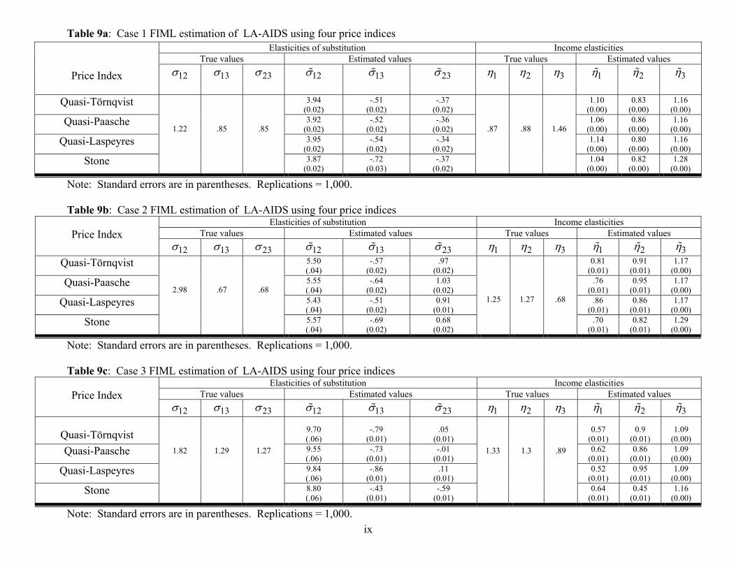
ix

Table 9a: Case 1 FIML estimation of LA-AIDS using four price indices


Price Index

12σ 13σ 23σ 12σ 13σ 23σ 1η 2η 3η 1η 2η 3η

Quasi-Törnqvist 3.94 (0.02)

-.51 (0.02)

-.37 (0.02)

1.10 (0.00)

0.83 (0.00)

1.16 (0.00)

Quasi-Paasche 3.92 (0.02)

-.52 (0.02)

-.36 (0.02)

1.06 (0.00)

0.86 (0.00)

1.16 (0.00)

Quasi-Laspeyres 3.95 (0.02)

-.54 (0.02)

-.34 (0.02)

1.14 (0.00)

0.80 (0.00)

1.16 (0.00)

Stone

1.22

.85

.85

3.87 (0.02)

-.72 (0.03)

-.37 (0.02)

.87

.88

1.46

1.04 (0.00)

0.82 (0.00)

1.28 (0.00)

Note: Standard errors are in parentheses. Replications = 1,000. Table 9b: Case 2 FIML estimation of LA-AIDS using four price indices

Elasticities of substitution Income elasticities True values Estimated values True values Estimated values Price Index

12σ 13σ 23σ 12σ 13σ 23σ 1η 2η 3η 1η 2η 3η

Quasi-Törnqvist 5.50 (.04)

-.57 (0.02)

.97 (0.02)

0.81 (0.01)

0.91 (0.01)

1.17 (0.00)

Quasi-Paasche 5.55 (.04)

-.64 (0.02)

1.03 (0.02)

.76 (0.01)

0.95 (0.01)

1.17 (0.00)

Quasi-Laspeyres 5.43 (.04)

-.51 (0.02)

0.91 (0.01)

.86 (0.01)

0.86 (0.01)

1.17 (0.00)

Stone

2.98

.67

.68

5.57 (.04)

-.69 (0.02)

0.68 (0.02)

1.25

1.27

.68

.70 (0.01)

0.82 (0.01)

1.29 (0.00)

Note: Standard errors are in parentheses. Replications = 1,000. Table 9c: Case 3 FIML estimation of LA-AIDS using four price indices

Elasticities of substitution Income elasticities True values Estimated values True values Estimated values Price Index

12σ 13σ 23σ 12σ 13σ 23σ 1η 2η 3η 1η 2η 3η


-.79 (0.01)

.05 (0.01)

0.57 (0.01)

0.9 (0.01)

1.09 (0.00)


-.73 (0.01)

-.01 (0.01)

0.62 (0.01)

0.86 (0.01)

1.09 (0.00)


-.86 (0.01)

.11 (0.01)

0.52 (0.01)

0.95 (0.01)

1.09 (0.00)

Stone

1.82

1.29

1.27

8.80 (.06)

-.43 (0.01)

-.59 (0.01)

1.33

1.3

.89

0.64 (0.01)

0.45 (0.01)

1.16 (0.00)

Note: Standard errors are in parentheses. Replications = 1,000.

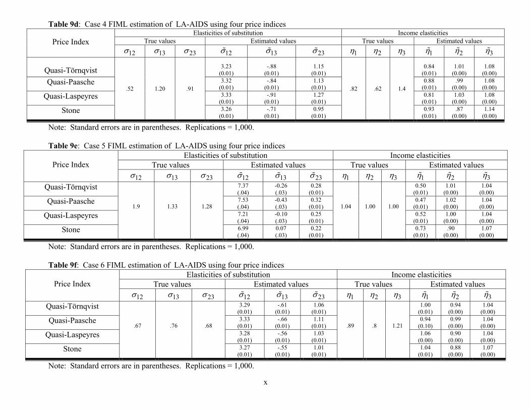
x

Table 9d: Case 4 FIML estimation of LA-AIDS using four price indices Elasticities of substitution Income elasticities

True values Estimated values True values Estimated values Price Index 12σ 13σ 23σ 12σ 13σ 23σ 1η 2η 3η 1η 2η 3η


-.88 (0.01)

1.15 (0.01)

0.84 (0.01)

1.01 (0.00)

1.08 (0.00)


-.84 (0.01)

1.13 (0.01)

0.88 (0.01)

.99 (0.00)

1.08 (0.00)


-.91 (0.01)

1.27 (0.01)

0.81 (0.01)

1.03 (0.00)

1.08 (0.00)

Stone

.52

1.20

.91

3.26 (0.01)

-.71 (0.01)

0.95 (0.01)

.82

.62

1.4

0.93 (0.01)

.87 (0.00)

1.14 (0.00)

Note: Standard errors are in parentheses. Replications = 1,000. Table 9e: Case 5 FIML estimation of LA-AIDS using four price indices


Price Index

12σ 13σ 23σ 12σ 13σ 23σ 1η 2η 3η 1η 2η 3η


-0.26 (.03)

0.28 (0.01)

0.50 (0.01)

1.01 (0.00)

1.04 (0.00)


-0.43 (.03)

0.32 (0.01)

0.47 (0.01)

1.02 (0.00)

1.04 (0.00)


-0.10 (.03)

0.25 (0.01)

0.52 (0.01)

1.00 (0.00)

1.04 (0.00)

Stone

1.9

1.33

1.28

6.99 (.04)

0.07 (.03)

0.22 (0.01)

1.04

1.00

1.00

0.73 (0.01)

.90 (0.00)

1.07 (0.00)

Note: Standard errors are in parentheses. Replications = 1,000. Table 9f: Case 6 FIML estimation of LA-AIDS using four price indices


Price Index

12σ 13σ 23σ 12σ 13σ 23σ 1η 2η 3η 1η 2η 3η


-.61 (0.01)

1.06 (0.01)

1.00 (0.01)

0.94 (0.00)

1.04 (0.00)


-.66 (0.01)

1.11 (0.01)

0.94 (0.10)

0.99 (0.00)

1.04 (0.00)


-.56 (0.01)

1.03 (0.01)

1.06 (0.00)

0.90 (0.00)

1.04 (0.00)

Stone

.67

.76

.68

3.27 (0.01)

-.55 (0.01)

1.01 (0.01)

.89

.8

1.21

1.04 (0.01)

0.88 (0.00)

1.07 (0.00)


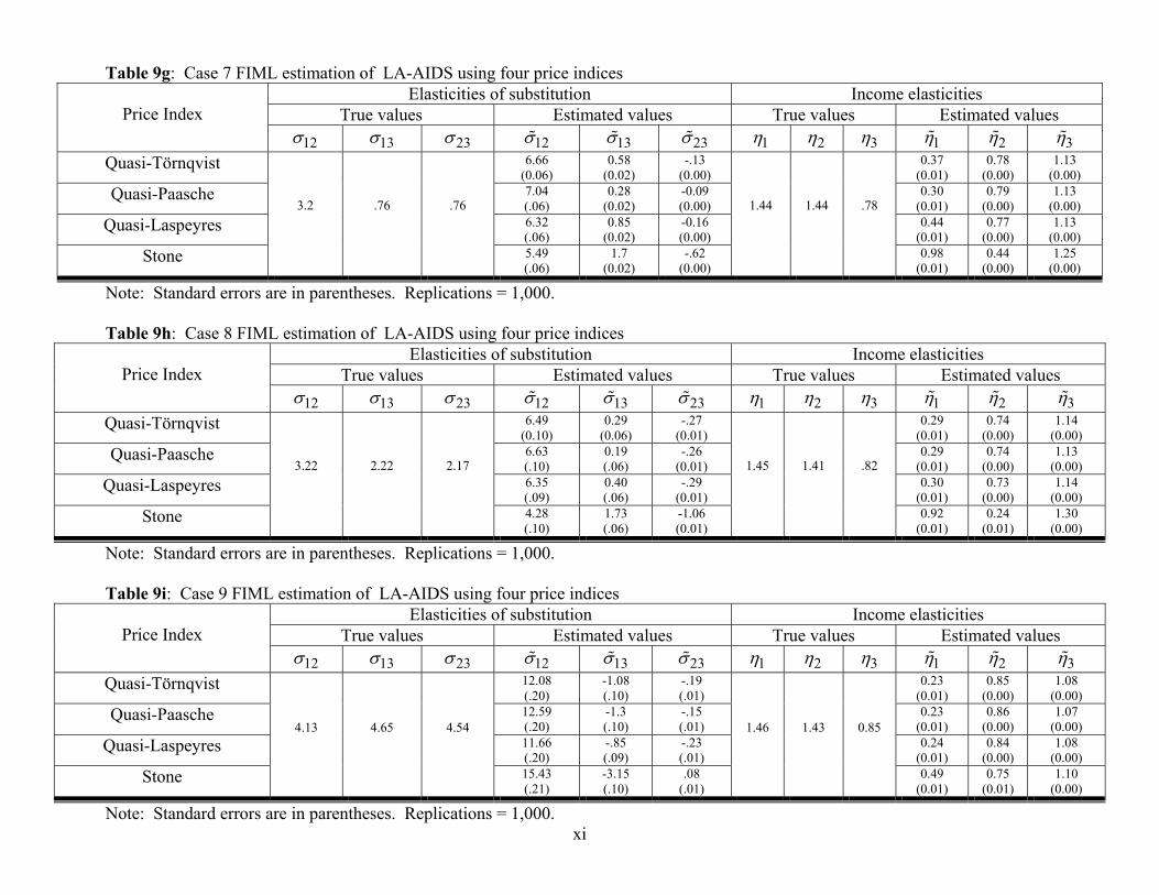
xi

Table 9g: Case 7 FIML estimation of LA-AIDS using four price indices


Price Index

12σ 13σ 23σ 12σ 13σ 23σ 1η 2η 3η 1η 2η 3η


0.58 (0.02)

-.13 (0.00)

0.37 (0.01)

0.78 (0.00)

1.13 (0.00)


0.28 (0.02)

-0.09 (0.00)

0.30 (0.01)

0.79 (0.00)

1.13 (0.00)


0.85 (0.02)

-0.16 (0.00)

0.44 (0.01)

0.77 (0.00)

1.13 (0.00)

Stone

3.2

.76

.76

5.49 (.06)

1.7 (0.02)

-.62 (0.00)

1.44

1.44

.78

0.98 (0.01)

0.44 (0.00)

1.25 (0.00)

Note: Standard errors are in parentheses. Replications = 1,000. Table 9h: Case 8 FIML estimation of LA-AIDS using four price indices


Price Index

12σ 13σ 23σ 12σ 13σ 23σ 1η 2η 3η 1η 2η 3η


0.29 (0.06)

-.27 (0.01)

0.29 (0.01)

0.74 (0.00)

1.14 (0.00)


0.19 (.06)

-.26 (0.01)

0.29 (0.01)

0.74 (0.00)

1.13 (0.00)


0.40 (.06)

-.29 (0.01)

0.30 (0.01)

0.73 (0.00)

1.14 (0.00)

Stone

3.22

2.22

2.17

4.28 (.10)

1.73 (.06)

-1.06 (0.01)

1.45

1.41

.82

0.92 (0.01)

0.24 (0.01)

1.30 (0.00)


Table 9i: Case 9 FIML estimation of LA-AIDS using four price indices


Price Index

12σ 13σ 23σ 12σ 13σ 23σ 1η 2η 3η 1η 2η 3η


-1.08 (.10)

-.19 (.01)

0.23 (0.01)

0.85 (0.00)

1.08 (0.00)


-1.3 (.10)

-.15 (.01)

0.23 (0.01)

0.86 (0.00)

1.07 (0.00)


-.85 (.09)

-.23 (.01)

0.24 (0.01)

0.84 (0.00)

1.08 (0.00)

Stone

4.13

4.65

4.54

15.43 (.21)

-3.15 (.10)

.08 (.01)

1.46

1.43

0.85

0.49 (0.01)

0.75 (0.01)

1.10 (0.00)


Rotterdam Model versus Almost Ideal Demand …kuwpaper/2006Papers/200605.pdfRotterdam Model versus...

Documents

Transcript of Rotterdam Model versus Almost Ideal Demand …kuwpaper/2006Papers/200605.pdfRotterdam Model versus...