1

ROTORDYNAMICS AND BALANCING REVISITED

Balancing of large, flexible rotors with significant body eccentricity

Zlatan Racic Marin Racic Z-R Consulting Z-R Consulting Bradenton, FL Hales Corners, WI zlatanraco@aol.com mzracic@gmail.com

ABSTRACT When working to balance newly manufactured rotors, current methods generally work well. New rotors are generally concentric and without distortions, and standard rotordynamics theories describe their behavior well. However, in the service industry, most rotors arrive with bows or deformations from many years of operation. When dealing with flexible rotors with significant mass eccentricities or bows (in excess of the “controlled initial unbalance” limits allowed by ISO 1940), current theories don’t fully address or explain their dynamic behavior. Furthermore, standard balancing methods often require excessive runs and encounter difficulties in meeting contracted balancing criteria. A new balancing procedure has been developed which allows successful multi-plane balancing (using 2N+1 balancing planes) of rigid or flexible rotors found to be outside ISO 1940 standards. The procedure utilizes measured runout eccentricities and FE-modeled rotor mode shapes for the selection of balancing planes. The majority of balancing is done on any common, high-speed balancing machine at not higher than 50% above the first system resonance. The key is separating “rigid mode” effects from resonant effects, and balancing each separately. The rigid modes are balanced using axially distributed weights, while the resonant modes are balanced only with modal weights in a zero-sum force and moment configuration. The end result is a “dynamically straight” rotor that remains balanced and has no distortion or bending at any speed. This method requires fewer runs, saving time and money, and the rotor is guaranteed not to need field balancing upon properly aligned installation. Key Words: Balancing; Eccentricity; Inertial force; Inertial mechanics; Precession; Rotor; Rotordynamics; Vibration ,

2

INTRODUCTION: Balancing technology is still relatively new. Thirty or forty years ago it was primarily still part of the skilled trade and was often obscured. In more recent years, balancing literature has proliferated, and numerous writings on general balancing and the balancing of flexible rotors can be found. The majority of papers and references are centered around the derivation of equations of motion based on a Jeffcott rotor model. These balancing concepts, developed as a result of theoretical work, have been able to satisfy most rotors’ balancing requirements, particularly for newly manufactured rotors. The original practical balancing guidelines and criteria were established by OEMs to deal with new rotors, and these OEM practices were subsequently transferred to industry. In practice, however, especially in the service industry, many rotors tend to be “difficult” to balance. New rotors generally don’t have the problems that service rotors encounter, and the OEMs’ standards and practices don’t translate well to rotors that have mass eccentricities in the form of bows, deformations, machining errors or other issues. The ever growing need in power generation to produce ever increasing megawatts has led to increasingly slender and flexible rotor design for turbines and generators. This increased flexibility can lead to difficulties in balancing, and especially when the rotors have been deformed outside their design tolerances. The manufacturing standards that have been created to classify and to deal with these and all rotors have been based on the machining accuracy, condition and dynamic behavior of newly manufactured rotors. Though not an exact application of Pareto’s 80/20 rule, the ratio seems to hold that at least 80% of newly manufactured rotors are in the expected condition (that is, their distributed mass eccentricity falls within the limits designated by ISO 1940 standards), and standard methods of balancing apply. The other 20% or so are considered from a standards point of view to be “exceptions” and are suggested to be dealt with on a case by case basis. However, when it comes to the service environment, all the rotors encountered have been running for some period of time, and through various operational issues or repairs, may have developed defects such as bows, bent couplings or other problems. Among these operational rotors handled in service repair facilities, the above ratio is reversed, and around 80% of these rotors are outside the manufacturing limits prescribed in ISO 1940, and behave as exceptions. As such, the standard balancing methods do not apply, or at the very least tend to encounter significant difficulties. When standard balancing methods are used (such as the N-method or N+2 method), even any rotor with mass eccentricity can eventually appear to be balanced perfectly well in a balancing facility, since it is operating in an uncoupled condition. However, when the balanced eccentric rotor is reinstalled in the field and coupled to other rotors, it very often has excessive vibration and doesn’t run as expected. Countless times, an argument develops where the service shop says, “It was balanced perfectly well over here, it must be your installation error,” while the plant replies, “We installed it correctly, so it must be your error in balancing.” In reality, both sides can be telling the truth, and the apparent error arises instead from a misunderstanding of rotordynamics behavior.

3

The goal of this paper is to qualitatively explain the rotordynamic behavior of flexible rotors with significant distributed mass eccentricity that can lead to the rotor’s inability to run when installed in the field, and to demonstrate a new balancing method that successfully balances any eccentric or bowed rotor, additionally guaranteeing that it will run smoothly when installed in the field. The Problem of Assumptions: All rotors used as tools for transmitting power are treated in textbooks as simple beams, or as massless shafts with attached point-masses. Many beam theories were developed in the past ((Timoshenko, Euler-Bernoulli), along with methods to calculate a rotor’s critical speeds and to predict its rotordynamic behavior (Prohl-Myklestad, Stodola-Vianello, Rayleigh, Ritz and FEA based). These theories and others are all founded on the assumption that a rotor acts at all times as a pure spring-and-mass system, and that its behavior is linear through its entire operating speed range. These theories also assume that the rotor mass is absolutely concentric. These assumptions are valid in practice for concentric rotors with negligible mass eccentricities within the limits of ISO 1940, and are perfectly valid in a wide range of cases. However, in the unique cases where a rotor has distributed mass eccentricity outside the limits of ISO 1940, these theories don’t fully explain the rotor’s behavior. When a rotor’s mass eccentricity exceeds the point where the dynamic contribution from that eccentricity is negligible, the rotor no longer behaves as a linear system. Additionally, at a speed above the rotor’s first system resonance frequency, it no longer behaves as a pure spring-mass system, but rather as a body governed by inertial forces. It is in this mode of behavior that balancing eccentric rotors becomes difficult. Balancing method descriptions almost always include the statement, “assuming that the rigid rotor unbalances have been solved.” However, it is the rigid rotor unbalances that in an eccentric rotor create the difficulties to begin with, and their full effect with regard to eccentric rotors is neglected in theories of rotor behavior and balancing. In the equation of motion of a spring-mass system, mass eccentricities are assumed to have the same effect as unbalance forces. However, for a significantly eccentric rotor, this is true only up to the rotor system’s first critical speed, but is not true at higher speeds. Above the first critical speed, the inertia of the eccentric mass becomes dominant over the spring force of the rotor system. Another incorrect assumption is that an eccentric rotor will spin about purely a single axis at all speeds. In practice, a rotor with distributed mass eccentricity naturally changes its axis of rotation (or precession) from its shaft axis (that is, the line connecting the two journal centers) to its central principal mass axis (that is, the line passing through the mean center of mass from all radial planes) as it passes through its first system critical

4

speed, and later at higher resonant frequencies. At lower speeds, the mass axis will technically be in precession around the shaft axis, though the rotation and precession will be synchronous and identical, and there really is no true separate precession. At higher speeds (above the first system resonance), the rotation and precession are still synchronous, but separate. The spinning of the rotor body remains around the shaft axis at all speeds, since the input torque always acts about this axis, while this shaft axis also at the same time precesses around the mass axis. In both cases, low, before the 1st system resonance, and high, above 1st 1st system resonance speed, the minimum amplitude measured is equal to the eccentricity excluding any rotor’s bending.

Figure 1: Sketch of the change in axis precession of a bowed rotor at the first critical speed, with the center shifting from the shaft axis to the mass axis.

5

The cause of this axis change is based within the asymmetric inertial forces generated from the mass eccentricity, due to the rotor tendency of self balancing above the first system critical. This will be explained in detail in the next section of the paper. A simple sketch showing the general idea of this change in axis is seen in Figure 1. (The way the figure is shown here is only applicable if spinning uncoupled in free-free mode; if coupled, other bending will likely occur). This change in axis is most readily visible when a rotor is spinning in a balancing bunker, and can be observed in the measured position of the shaft centerline. In a balancing facility, if an eccentric rotor is brought up to speed while uncoupled (free-free mode), its rotation will switch at the first critical speed from being centered at the shaft axis, to a precession of the shaft axis around the now-centered mass axis (or, will switch to the maximum extent allowed by the bearing clearances, in case the eccentricity distribution is particularly skewed or large). Any balancing weights that are subsequently placed based on readings above the first critical will inadvertently balance the rotor around its mass axis, since the mass axis will have become the center of precession of the shaft axis. Any measured responses of displacements or bearing forces will likewise be based on the rotor’s rotation about its mass axis. These responses can appear to be within tolerance criteria in the bunker, making the rotor appear to be well balanced, but the rotor will likely not run well when installed in the field and spin constrained around a “forced” axis. After being balanced around its mass axis, if the rotor is reinstalled in the field and coupled to other rotors, its rotation (and any precession) will be constrained to its shaft axis at all speeds. In this situation, the mass eccentricity itself along with the installed balance weights will now all act as unbalance forces on the rotor, since the rotor has not been balanced around its shaft axis. This will create very high vibrations in the rotor train. The solution is to first balance a rotor with eccentricity in a way that balance weights are distributed to counteract unbalance forces from the distributed mass eccentricity, such that the overall central principal mass axis is shifted to be fully coincidental to the shaft axis, while also not causing any new rotor bending (meaning that no unresolved moments were left on rotor). This will prevent the change in rotational axis from occurring (since now there is effectively only one axis to deal with). This will also solve the “rigid mode” forces (this will be described in more detail later). Any remaining unbalance effects at higher speeds can be balanced if needed using purely modal weights (so that no new moments are created from modal bending). When installed in the field, the rotor will naturally spin around its shaft axis at any speed, and provided it is installed with correct alignment, the rotor is guaranteed to run smoothly in the field. To get the proper balancing weight distribution, an eccentric rotor must be balanced in a minimum of 2N+1 balancing planes (where N is the highest mode the rotor reaches at

6

operating speed). It is well known that any fully rigid rotor can be balanced in any two planes. Any flexible rotor can be divided into shorter sections or “modal elements” such that each element acts as a rigid body at frequency of its’ critical speed. By balancing the mass eccentricity and unbalance of each rigid element in two planes (each non-open-end plane of the rotor is shared by two elements, since the elements are adjacent), and by proper axial distribution of the weights, placed in planes selected based on rotor’s highest mode, within its’ operating range the unbalance effect from the mass eccentricity (that is, the “rigid mode” responses) can be compensated for and fully eliminated for all speeds. Before moving on, it should be remembered that the general definition of a balanced rotor is that the rotor produces zero dynamic forces at the bearings, and not necessarily zero displacement. Also, an ideally balanced eccentric rotor, for which the axial distribution of unbalance is known, would be balanced in an infinite number of balancing planes (Federn). Only then would the rotor’s mass axis be brought exactly coincidental to the rotor’s shaft axis. This would mean that ALL unbalances are compensated for with forces from balancing weights, such that none would be excited at the respective resonant speeds, and that there would be no unresolved internal moments left on the rotor. The author has developed a balancing procedure to select the balancing planes and ensure proper weight distribution to remove the effects of any rotor body eccentricity (referring to the rotor mass between the bearings), and thus the effect of inertial forces at higher speeds. The full balancing procedure can be completed at less than 50% above the first system critical speed. Thus, it is given the name, Quasi-High Speed Balancing Method (QHSBM). A detailed explanation of this new balancing method in high speed balancing facility for large turbine generator rotors is described in the second half of this paper. ROTORDYNAMIC BEHAVIOR OF ECCENTRIC ROTORS: Before delving into the explanations, some terminology should be clarified first: As mentioned earlier, the rotor’s shaft axis (torque axis, or shaft centerline, or geometric axis, or design axis) is the line connecting the center of the journals, and is the axis the rotor is intended by design to spin around. The rotor’s mass axis (or principal mass axis) is meant as the mean straight line passing through the center of the mass of each radial plane of the rotor. The rotor’s torque axis is the center of where the input torque is applied (via a coupling), and it is the torque axis that truly defines a rotor’s rotational axis. In this paper, the torque axis is assumed to always be the shaft axis, although errors in machining or couplings or alignment can cause this to not always be the case in real life. Any rotor always spins at all times and speeds around its torque axis. However, this torque axis itself can be in synchronous precession around the mass axis at higher rotational speeds. The “rigid modes” of the rotor refer to the motion of the rotor as a fully rigid beam without any bending. There are two rigid modes, lateral and rocking. The lateral rigid

7

mode is vibration displacement of the rotor only parallel to the shaft axis. The rocking rigid mode is as it sounds – a tilting vibration displacement of the rotor around its center of gravity. These two rigid modes should not be confused with the first and second critical speed rotor responses that have similar motions but may have some additional rotor’s elastic bending. The lateral and rocking rigid modes arise from the centrifugal force from a rotor’s eccentricity, and can be present at all rotational speeds of an eccentric rotor. These rigid modes are not present on a non-eccentric rotor. The rigid mode responses steadily increase with increasing rotor speed (they can be seen as a constant up-sloping amplitude line on a Bode plot, starting from very low speed). In contrast, the first and second critical speed modes are only defined at resonance and are independent of any additional forcing function besides the original unbalance. A static unbalance is one that causes the mass axis to be displaced only parallel to the shaft axis (for example, this could be an eccentricity distributed equally along the full length of the rotor). This causes the lateral rigid mode, which can also be called the “static response” usually at very low speeds but on sufficiently soft bearings. A couple unbalance is one that causes the mass axis to be tilted while still intersecting the shaft axis at the axial center of gravity of the rotor (this exact situation is almost never seen on real rotors). A quasi-static unbalance is one that causes the mass axis to be both laterally displaced and tilted with regard to the shaft axis, such that the mass axis intersects the shaft axis at some point other than the rotor’s axial geometric center. This is the most common real situation, and is the case dealt with in this paper. The phrase “bending modes” is used here to refer to any shaft-bending component of the first and second critical speed resonance responses (though these are not true bending modes, as the bending depends on the bearing stiffness), or to the third critical speed response (which is the first true bending mode of the rotor, being intrinsic to the geometry of the rotor shaft alone, and not dependent on the bearings). The purpose is that to understand the behavior of an eccentric rotor and to balance it properly, the purely rigid body effects must be dealt with first, ideally fully separately from any bending effects from the rotor’s flexibility. In real practical life, as in the case in a balancing bunker, some flexing is allowed ,as it will be seen later. Natural Behavior of an Eccentric Rotor: Ideally, if unconstrained, any rotor will want to naturally spin about its mass axis. In a perfectly concentric rotor, this mass axis would coincide with the shaft axis, and the rotor would naturally spin around the shaft axis at all speeds, as it was designed to. Traditional rotor balancing theory would apply in this case.

8

Where things get interesting is when looking at an eccentric rotor with quasi-static distributed unbalance (typically a shaft bow or machined eccentricity), where the rotor is constrained to spin about its shaft axis (in noncentroidal rotation). In this state, there are numerous aspects of the rotor’s behavior that need to be separated and dealt with individually for the purposes of balancing. In an eccentric rotor, the natural tendency would be to rotate about the mass axis, which would not coincide with the shaft axis. If it spun freely this way, the rotor would be absolutely “self-balanced”, without transmitting any forces (with measured displacement equal to the measured rigid mode eccentricities). However, this tendency is constrained at lower rotation speeds (below the first critical speed) by gravity holding it in the bearings, by the spring forces within the bearings and the rotor body itself, and by the applied torque acting along its shaft centerline. This is the region where the spring-mass system governs the rotor behavior, and in which the system acts linearly. Ultimately, an eccentric rotor’s behavior is dependant on many variables, such as the level of shaft flexibility, the stiffness of the bearings, the bearing clearances, the distribution of the eccentricity, and whether it is coupled to another mass (rotor). These variables can dictate how the rigid mode responses will be manifested in the rotor. The forces causing the rigid mode responses will be present regardless. If the rotor is relatively free to move, the forces will be seen as rigid mode displacements. If the rotor is constrained by the bearings, the displacement will be low, and the forces will be seen as high stress in the bearings. In either situation, the tendency remains for the rotor to switch its rotational axis as it reaches the first critical speed. During this flip in axis, the position of the rotor in space changes, and depending on the bearing constraints, the rotor displacement may be instead converted into and seen as bearing forces. The total energy to be dissipated in the system remains constant, however. The Two Axes: Here is a more detailed, qualitative look at the change in rotational axis described earlier. In general, a rotor with significant mass eccentricity can be thought to rotate around two different axes within the operating range, with the axis depending on rotational speed. Or more accurately stated, (at any one time) there is an axis of rotation and a synchronous axis of precession. When driven up in speed, the rotor first starts spinning around its shaft axis. The mass axis is essentially precessing around the shaft axis, as the eccentricity (or “high point” spins around with the rotor body. Then as it passes through the first critical speed, the rotation “flips” to the mass axis. Here, the shaft axis (essentially the whole rotor body) is synchronously precessing around the mass axis, while rotation is still continuing about the shaft axis (or axis of torque). When the rotor decelerates or freewheels down, the rotor follows the same pattern, flipping from its mass axis back to its shaft axis, although since there is now an absence of torque, the rotor’s shaft centerline position in space (relative to the 0-0 journal reference point) may be

9

different (as hysteresis) when this flip in axis takes place on coastdown. The input torque itself can act as a constraint to the position of the rotational axis. A drawing of a shaft-centerline plot can be seen in Figure 2. This sketch shows a generic shaft centerline plot representing the shaft centerline(s)’ position with increasing speed. At the different speeds, a representation of the centerline’s orbit is shown. There are actually two different centerlines being followed through the speed range. At lower speeds, the centerline of the orbit shown is the actual shaft axis. At higher speeds (above the first system resonance), the centerline of the orbit shown is actually the mass axis. The smaller orbits above the first critical represent the effect of the “self-balancing mode,” where the rotor response lags the outward force from the inertia of the eccentricity by 180 degrees, offsetting its effect. Any subsequent phase shift of rotor passing through higher modes is done about the rotor’s mass axis. With every phase shift, mass centerline may assume a different place in reference to the original coordinate axis.

10

Figure 2: Sketch showing a generic shaft centerline plot, following the shaft centerline(s)’ static position as it changes with speed. At low speed, the centerline is truly the shaft axis, while at high speed the centerline is really the mass axis. In both cases, the orbits shown represent what would be measured by shaft displacement probes. Of course, the probes and software cannot distinguish between an orbit generated by precession of the mass axis or precession of the shaft axis, and in both cases, the orbit dimension would be a sum of both the deflection from unbalance response and the size of the mass eccentricity. Note that the slight change drawn here in the direction of the shaft centerline path at the critical speed represents the flipping of the axes and the associated change in position of the centerlines; this path change can in reality go in any direction on a real rotor, and is not predictable. Both the motion of the shaft axis and the motion of the mass axis are occurring synchronously at the same time. For the sake of a simple visualization only, this precession relationship is not unlike the motion of the earth, moon and sun (the mechanics are wholly different, of course). The moon is spinning synchronously with regard to the earth while orbiting (precessing) around the earth, while the earth is also orbiting around the sun. Visualizing the low speed rotor situation, the moon is like the mass axis precession, the earth is like the shaft axis, which has its own orbit around the sun and is also spinning (albeit not synchronously with regard its orbit around the sun), and the sun would be like the coordinate center of the shaft axis orbit. (It should be noted: For each orbit showing mass axis precession, there is truly also an orbit of the shaft centerline (shaft axis) as well but that isn’t drawn; it would be drawn within the mass axis orbit and be of the same shape, with elliptical radii equal to the mass axis orbit, less the peak distance measure of the eccentricity. The same thing applies to the shaft axis precession orbit; there could be drawn the smaller mass axis orbit within it. For the sake of a less messy drawing, these orbits are left off.) To further clarify, the starting axis (shaft axis) is the initial center of rotation that the torque is (assumed in this case to be) applied to (with a 0-0 coordinate reference being at the center of the journals), and the rotor’s motion in this rotational axis is dominated by spring and mass forces. This means that the rotor’s motion is in the same direction as the unbalance force (from the eccentricity), or that the rotor’s motion is in phase with the force applied. When in its shaft axis, the eccentricity (“high point” of the surface) will spin around with the rotor and will always be the same distance away from the center of rotation (which is the shaft axis), assuming there is no any additional rotor elastic bending. Or in other words, the mass axis is precessing about the shaft axis. The force arising from the inertia of the mass eccentricity will create lateral rigid mode vibration, which acts to pull the rotor outward as it spins, in the direction of the eccentricity (or mass axis).

11

The second axis around which the rotor’s rotation (or rather, precession) is centered above the first system resonance (critical) speed is the mean line through the center of mass. In this axis, the direction of the rotor’s motion is lagging (theoretically) 180 degrees behind the direction of the unbalance force from the eccentricity. This in effect self-balances the lateral rigid mode of the rotor around the mass axis (the rocking rigid mode, if present, would remain, and be observed at higher speed). Also, in reality, this “flip” angle need not be exactly 180 degrees, but can vary somewhat depending on the ratio of the unbalance caused by eccentricity and the amount and direction of other unbalances on a rotor. While the shaft axis is precessing about the mass axis, the rest of the rotor body now essentially acts as the “high point” and spins around this new mass-center of rotation as referenced from the initial coordinate axis (this new axis from here on becomes the new reference for the center of rotation). For a rotor spinning in free-free mode this change is easy to visualize. But when the same rotor is spinning in a constrained state coupled within a multi-rotor train, its operating deflection shape can be difficult to visualize. It is necessary to keep in mind the overall level of rigidity or flexibility of the rotor in question, or the amount of flexing of any particular sections of the rotor between the bearings. The change in axis occurs, as mentioned, through the first critical speed. However, the change itself actually occurs a little before or a little after the actual critical speed, depending on the distribution of the eccentricity and a damping of the system. In the case of a bend or a bow, where the eccentricity is higher in the center and drops to nearly zero at the rotor ends, the flip in axis occurs after the first critical speed, and in this case, any residual displacement residual amplitude is actually rotor eccentricity! In the case of a distributed mass eccentricity along the length of the rotor, the flip in axis occurs before the first critical speed and any residual displacement amplitude is actually a residual unbalance. Furthermore, after the flipping of the axes at around the first critical speed, it is also important to note that the position of the mass axis does not necessarily then stay in its new place through the rest of the speed range. If higher critical speed responses or residual rigid mode effects induce bending in the rotor, this bending will act to again shift the mass centerline. The shaft axis will still continue its precession around the mass axis, but the overall position of the rotor (and the magnitude of the transmitted forces) relative to the bearings may continue to change as the rotor passes through higher speeds. This can all be seen in a Bode plot. The flip in axis is seen as a drop in rotor vibration amplitude, accompanied by a phase shift, as the lateral rigid mode is momentarily self-balanced just before or after the first critical resonance response appears. (A side note: the first critical resonance response is actually excited by the lateral rigid mode

12

unbalance; if the lateral rigid mode is fully balanced and compensated for, the first critical resonance response will not appear). If there are no other unresolved unbalances or internal moments, then the amplitude will remain constant at the level of the eccentricity for all higher speeds. This demonstrates that the vibration amplitude of a perfectly balanced eccentric rotor can not be reduced any lower than the value of the rotor’s eccentricity. The vibration amplitude readings can actually be reduced, but only in a false manner by intentionally unbalancing the rotor, such that the shaft displacements at the bearings are converted instead into new forces pounding the bearings. Obviously, this is not a desired solution to reduce vibration amplitudes. The measured vibration amplitudes can also appear to be smaller than the true level of eccentricity because of the choice of measuring location, especially if the location is far away from the axial center of gravity of a rotor that is elastically sagging due to gravity. It should also be noted that an eccentric rotor requires constant additional torque to maintain constant-speed rotation, as compared to a concentric rotor. The constant force resulting from momentum acting outward on the eccentric mass of the rotor causes either extra flexing of the rotor (more so for flexible rotors), or causes a continuous extra, cyclic “push” into the bearings (more so for rigid rotors). This cyclic bearing stress or rotor flexing must originate from the original input energy of the rotor. As this force is dissipated into the bearing, additional energy in the form of extra torque is needed to maintain the rotor’s speed, beyond the amount of torque needed to overcome standard friction and windage losses. Another Visualization: To better understand the dynamics occurring in the lateral rigid mode of an eccentric rotor, it may be helpful to visualize the rotational axes and the centrifugal force effects in a simpler picture. In the case of a (rigid mode) rotor rotating freely unconstrained, it might be easier to first imagine a spinning, two-blade propeller with one blade significantly heavier than the other (say, with one wooden blade and one steel blade, and in the absence of gravity). Imagine the propeller’s rotation is frictionless, and is initially about its geometric center (its mounting point), and that its mount is held in a fixed, stationary position, allowing no vibration. As it spins, the unequal momentum of the propeller blades will exert forces on its mount, in the net direction of the steel blade (in response to the centripetal force exerted by the mount). This is a result of the blades’ constituent particles’ inertia, wanting to move in a straight line in space, but being constantly accelerated radially inward through the eccentric mass toward the center of rotation, by centripetal force (that is, the angle of all particles’ velocity vectors is being continually turned to follow the circular path of motion).

13

Because the inertia of the two blades is different, there will be a constant force exerted on the propeller’s mount. If this is a fully closed system, then all the energy is conserved. Both force (internal stress on the mount) and rotation (or motion), originate from the same original sum total of energy within the system. Any subsequent change in rotational velocity requires an equivalent change in forces within the system (a conversion between kinetic and potential energy). If the net centrifugal force is continuously exerted as a stress force on the mount (that is, the propeller isn’t balanced in its rotation), the energy utilized in producing this force on the mount is equivalently reduced in the energy (and hence, rotating speed) of the blades’ motion. The blades would slow down steadily over time. This effect is solely because of the unbalanced rotation about a forced geometric axis, as opposed to an axis located at the propeller’s center of mass. Now, let us imagine that the propeller’s mount is suddenly removed, and the propeller is left to spin freely unconstrained (still ignoring gravity). The net inertia of the blade wouldn’t change (nor momentum, which is conserved), even though the rotational motion would instantly change. Given the difference in masses of the blades, the inertia of the particles in the steel blade would be much greater than the inertia of the wooden blade. The blade’s rotation will flip to a rotational axis such that the inertia of each particle of the blade will be balanced by the net inertia of another particle (or particles) of the blade on the opposite side of the new rotational axis. Or put another way, at the moment of release, the point of the overall center of mass (on the propeller’s rotational plane) would stay stationary in space, and would instantly (no damping considered) become the propeller’s new axis of rotation. Or, it could also be said that the propeller’s original axis of rotation is now precessing around the center of mass. (However, unlike an eccentric rotor, there is no rotation still occurring around the original rotation point, since there is no torque applied there.) The net rotational velocity about its axis would remain constant as well. Since momentum is conserved, the difference in inertia of the two blades would be converted into a difference in velocity between the blades, by virtue of the wooden blade now being farther from the new axis of rotation than the steel blade, while maintaining circular motion. Now, let us imagine this above scenario taking place within each radial plane of a cylindrical, rigid rotor, rotating at a relatively low speed (well below the first critical speed). First, let us imagine a rotor that is perfectly concentric and rotating about its own shaft axis, and that the rotor is fully constrained within two bearings.

14

It would rotate smoothly, and if the bearings were instantly removed, the rotation of the rotor would remain unchanged. This scenario also demonstrates that there would have been no forces exerted on the bearings. By definition, the rotor is perfectly balanced. Now let us imagine this rigid rotor as having an evenly distributed body mass eccentricity (as a static unbalance), and imagine again that it is rotating fully constrained within two fully rigid, stationary bearings (assuming straight concentric journals, such that the forced rotation of the rotor is about its shaft axis). In a similar manner as in the propeller example, the rigid rotor would exert a force against the bearings, with the net direction of the force being identical to the direction of the sum of all vectors drawn from the shaft centerline to the rotor’s center of mass in every radial plane. Even if there is no motion at the bearings, the tendency of the inertia of the eccentric portion of the rotor to asymmetrically “pull” the rotor radially outward would create a continuous synchronous dynamic force on the bearings. The rotor in this case is clearly not balanced. Since the rotor is fully constrained by its bearings, the “vibration” of the rotor if measured at the journals would appear to be zero, if based on displacement measurements alone. It might wrongly appear to be perfectly balanced. Meanwhile, force measurements at the bearings would show very high force levels. If these bearings were instantly removed (imaging the rotor in space), the rotor would instantly shift its rotational axis to the mean straight line of the center of mass of each radial plane of the rotor. The journal centers would no longer be in the axis of rotation, and an otherwise stationary probe placed at the journals would measure “vibration.” However, the rotor would not be experiencing true vibration at this point, and would actually be perfectly balanced as it would be spinning freely about its mass axis. The rotor wouldn’t bend or change shape in any way, and would be in a state of “dynamic equilibrium.” If the journals were straightened and their centers repositioned to line up with this mass axis line, and these journals were again placed within bearings, the bearings would once again experience no forces. BALANCING CONSIDERATIONS FOR ECCENTRIC ROTORS: The conclusion from the situations described so far is that a rotor will naturally want to spin around its center-of-mass axis in free space, and that any rotor spinning in that axis will be naturally balanced and will not transmit forces to its bearings. A goal of balancing any eccentric rotor, therefore, should be to use balance weights to bring the rotor’s mass axis into alignment with the rotor’s shaft axis. However, it is imperative that the correct axial distribution of balancing weights is utilized to accomplish this.

15

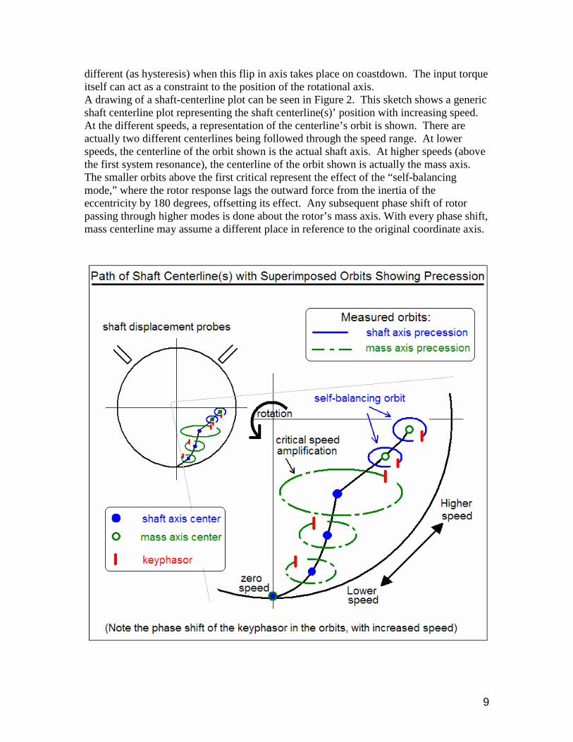
Of course, when approaching an eccentric rotor to be balanced, the true shape of the eccentricity is unknown. Taking detailed runout readings in practice is a crucial first clue to the weight distribution that might be needed, and to recognize the smallest vibration amplitudes obtainable given the eccentricity. While attempting to “mirror” the distribution of the mass eccentricity by placing balance weights, the distribution of the eccentricity can only be inferred by the rotor’s measured behavior. This brings up another important concept. The purpose of compensating for the eccentricity in multiple balancing planes is to essentially create a “mirror image” of sorts of the mass eccentricity. See the image below. If the shape and amount of the eccentricity is mirrored by the balancing weights, then the rotor will be “dynamically straight” in operation at any speed. This means that the rotor will not change shape or bend, regardless of speed (excluding any other random unbalance).This is the most critical requirement to successfully balance an eccentric rotor.

Figure 3: Distribution of balancing weights mirror the shape of the eccentricity

Shifting the center of mass of the rotor into the shaft axis is not sufficient on its own without proper axial weight distribution. A concentrated weight at one or two planes could shift the mass axis toward the shaft axis as well. However, a concentrated weight would create bending at higher speeds due to creating a high localized centrifugal force. Furthermore, a concentrated weight or two would invariably introduce internal moments into the rotor. While concentrated weights could possibly reduce the rigid lateral mode and the flip in axis, the rigid rocking mode would be worsened. Therefore, it could be more accurately considered that the mass axis isn’t actually being moved or shifted to the shaft axis. Rather, the properly axially distributed weights are creating a compliment to the mass eccentricity, utilizing balancing weights at a certain distance to create a certain force to be opposite and equivalent to the forces created by the mass eccentricity. Only by this method can a rotor that is dynamically straight be achieved. Rigid Modes versus Resonant Modes, Revisited: Rigid rotor modes are often negligible on concentric rotors, but have a large effect in balancing eccentric rotors. Recall that that there are two purely rigid modes of a rotor: a lateral (translational) mode and a rocking (pivoting mode). Within the operating speed range of power generation rotors, there are also typically up to three resonant mode

16

responses that occur at their respective critical speeds. The first two resonant responses (the so-called first and second mode responses) are connected to the presence of the two rigid modes, but when dealing with eccentric rotors, these must be viewed separately. The third mode resonant response is the first true bending mode, where two nodal points will always occur between the bearings, and where the rotor shaft intrinsically bends independent of bearing stiffness. Rigid Modes: It is possible to have first and second (and third) mode resonant responses without having purely rigid mode responses present. However, it is not possible to have only the rigid mode response without also exciting resonant mode responses at their respective critical speeds. However, by properly balancing the rigid mode response, the first and second mode resonant responses can often be eliminated at the same time. Eccentric rotors demonstrate both rigid mode behavior and resonant mode behavior. The rigid rotor modes are based and originate entirely within the shaft. The rigid mode behavior is typically the best observed at low speeds, where the rotor behaves as a purely rigid, unbending beam. That is not to say that the rotor in this state won’t ever exhibit some flexing as well, particularly if it is coupled to other rotors, although the source of the motion would still be from rigid mode behavior. The rigid modes of an eccentric rotor can be seen regardless of speed, as their source is from centrifugal force from unbalance, and not from a resonance excitation. However, to be seen, the unbalance must be a distributed eccentricity (like a bowed shaft), to produce a large enough centrifugal force. A simple point mass unbalance will not induce rigid mode behavior, as the resultant centrifugal forces generally do not get large enough. The asymmetric momentum from sufficiently large mass eccentricity will result in increasing force with the square of rotational speed. This force will then be apparent as either steadily increasing vibration amplitude, from a speed of zero on up, or as steadily increasing bearing forces. A typical Bode plot showing this can be seen in Figure 4.

17

Figure 4: Bode plot showing steady up-sloping amplitude from rigid mode, with first and second critical speed responses added on top at the respective critical speeds. Which type or response is seen depends on the constraint of the bearings and the distribution of the eccentricity. If the mass axis is particularly skewed, the rotor will want to operate in that skewed line, but will likely find the bearing constraining its motion. In this case, the force will find its outlet as potential energy via a pounding or pushing force in the bearings. If the mass axis is more parallel to the shaft, then the bearing clearances will allow the force to find its outlet as kinetic energy via increased shaft amplitude with speed. Additionally, the all-speed visibility of these lateral or rocking modes within an eccentric rotor is dependent on the overall system damping. If the bearings are particularly stiff and have only marginal damping, then the response of these modes can be quite high. If the bearings are soft with a lot of damping, then these modes may not be seen at all. Due to the variability in the type of observed presence of the rigid modes, it is important for balancing purposes to measure both shaft amplitudes and bearing forces. Focusing only on one or the other can create misinformation regarding the state of balance of the rotor. Ultimately, the rigid modes unbalance can be solved using the principles of statics, viewing the rotor as a simple beam under distributed forces. Balancing weights need only be applied and distributed on the side of the rotor opposite the net eccentricity, such that the centrifugal force of the weights will equal the centrifugal force from the eccentricity. In balancing an eccentric rotor, this static solution MUST be completed first before dealing with any other resonant responses, and must compensate for both unbalance forces and moments. This ensures that the rotor becomes dynamically straight

18

at all speeds (does not bend). Very often, the resonant responses will end up being solved as well, or at least greatly reduced with the application of the correct static solution. A rigid rotor (or a rigid section, or “modal element” of an otherwise flexible rotor), regardless of speed, can be balanced in 2 planes. Once the rotor (or each of its elements) is properly balanced in 2 planes, the rotor can run at any speed and remain balanced. A rigid rotor (or a rigid element of a flexible rotor) stays rigid and balanced regardless of speed. This is the key principle utilized in the Quasi-High Speed Balancing Method described later. Resonant Modes: In contrast to the rigid modes, the resonant response modes are seen only at their respective critical speeds, and are based on the increased response due to amplification from an excitation force (such as unbalance) at that given speed. However, as mentioned earlier, unbalance from eccentricity that causes the rigid mode responses will also act to excite the first or second mode resonant responses, which will then act as an amplification of the same rotor motion caused by the rigid modes. A quasi-static eccentricity will excite both first and second resonant modes. At the second critical speed, the eccentricity that causes the rocking rigid mode will excite the S-mode shape response. A purely static eccentricity will excite only the first resonant mode, but not the second resonant mode (since the unbalance will be symmetric about that mode’s nodal point; there will also be no rigid rocking mode). Whether these resonant modes’ excitation responses appear more as rigid-like translation, or rocking, or as bending in the familiar first and second mode shapes, depends on the level of damping and the ratio of stiffness between the bearings and the shaft. Higher bearing stiffness will result in more of a bending response, while higher shaft stiffness will produce more of a rigid-beam type of response. If the rotor is fully concentric, there will likely be no noticeable rigid mode behavior (lateral or rocking). In a concentric rotor, the first appreciable vibration will then not occur until the first critical speed, when whatever residual unbalance exists on the rotor (not a bow or eccentricity) excites the first mode shape. After passing through the first critical speed, the concentric rotor’s vibration returns to zero until reaching the second critical speed. If there is no unbalance on a concentric rotor, then both the first and second critical speeds can pass by without resonant excitation. The only way to see their existence would be by observing the phase shifts. Above these first two resonant modes, on either an eccentric or concentric rotor, there is the first flexural mode or first bending critical (also often called the third critical). This

19

third critical is the first mode at which the shaft itself is actually inherently bending internally, with nodal points between the bearings. The frequency or eigenvalues (rotor speed) at which the third critical occurs is completely independent of the bearing supports. This is in contrast to the first two critical speed resonant responses, where the speed at which they occur and their responses are both bearing (support) stiffness dependent. Although the third critical inherently bends the rotor, the specific shape (eigenvector) of the bending still depends on the bearing stiffness. In soft bearings, the resultant shape has only a single bend in the center. In rigid (stiff) bearings, the shape will include some bending at the ends of the rotor as well, since the ends are constrained in the bearings. After completely balancing the rigid modes, it is sometimes seen that there are still resonant responses at the second and third critical speeds. These responses can possibly come from other residual point-mass unbalances, but more typically are caused by long overhangs outside the bearings that have some flexible bending behavior of their own. If the long overhangs cause a resonant excitation of the second mode, the vibration at the ends of the rotors will be seen to be 180 degrees out of phase with each other. If the overhangs excite the third mode, the vibration responses at the rotor ends will be in phase with each other. If the rigid modes are not completely balanced, then the overall motion of the rotor will be a combination of the resonant speed responses (at the critical speeds) and the rigid mode responses (present through all speeds). Again, this is most readily recognized by looking at the amplitude response on a Bode and Nyquist plots. The rigid mode component of the rotor’s motion will be seen as an up-sloping line through the entire speed range, while the resonant mode responses will be seen as spikes in amplitude on top of this line, at the critical speeds. The Overall Balancing Concept for Eccentric Rotors: It is essential that the rigid modes must be balanced and resolved first, before dealing with the bending modes. This assures that the shaft axis and mass axis become coincidental, and prevents all of the effects from the rotor’s change in rotation axis at the first system critical speed. More accurately, it prevents any visible change in axis from occurring. This prevents the mass eccentricity from inducing any additional bending in the rotor from its centrifugal force at higher speeds (assuming the shaft has some flexibility), and the rotor will behave like a concentric static beam. Or stated another way, it assures that the rotor will operate dynamically straight through the entire operating speed range. It can be assured that the rigid modes are balanced when the bearing forces are zero (or minimized to practical values) at all speeds, other than possibly at the rotor’s critical speeds. The rotor will behave as a linear system, and standard balancing procedures would now apply from this point forward.

20

After the rigid mode is resolved, any additional resonance responses must be balanced using only purely modal weights. This generally takes the form of an S-shot for a second mode or out-of-phase response, or a V-shot for a third mode or in-phase response). These modal shots are defined as weight distributions such that the sum of all forces and moments produced by the weights equals zero (ΣF = 0 and ΣM = 0). This is essential so as not to disrupt the rigid mode balance solution by adding new forces or moments that would act to re-shift the mass axis away from the shaft axis. In the placement of the modal weights in these distributions, the “acting” nominal weights should be at the point(s) of maximum rotor deflection(s) of the particular mode being balanced and compensating weights must be placed at the nodal points of the mode, so as not to disturb the rigid mode solution. The resolution of the remaining resonance responses should be relatively straightforward, after the effects of the rigid mode behavior have been removed. A Comparison of Balancing Methods: There are today, in principle, only two balancing methods generally used for balancing flexible rotors (in free-free mode) in a high speed balancing facility or balancing bunker. An example of the typical highly-eccentric rotor balancing results of these methods, and the new 2N+1 method (or QHSBM), is shown next. The following images are for the simulated balancing of an 800MW, 165,000 pound generator rotor (with a length of 515 inches and bearing span of 337 inches) that passes through three critical speeds up to 3600rpm. For the purpose of this comparison of methods, the rotor model was given a tapered, distributed mass eccentricity from zero to five mils (the model of the rotor can be seen earlier in Figure 3). The actual balancing process and results for the real rotor is presented in the final section of the paper. N-Method: The first is the so-called N-method, advocated by Bishop and Caldwell (developed in the USA), where N indicates the number of balancing planes, which corresponds to the highest critical speed reached in the rotor’s operating speed range. For example, a rotor passing through three critical speeds requires only three balancing planes. This method does not consider any rigid mode unbalances. The N-method is based around the needs of an OEM manufacturing environment, where quality control assures that the new machined rotors have no eccentricity or are within the tolerances of ISO 1940. However, balancing becomes a frustrating activity when the N-method is applied to balancing rotors with bows or other eccentricities outside the prescribed tolerances. This was recognized even by Bishop. While defending the position that only one plane per rotor mode is sufficient to balance any flexible rotor, he did not skip mentioning that rotors which exhibit difficulties during balancing are treated on a case by case basis. The end result of balancing very flexible, significantly eccentric rotors by the N-method is that the rotor operates in a contorted shape and produces larger forces on the bearings. The single concentrated weight used at the midplane to balance the first mode response will end up bending the rotor at higher speeds. An example of this contorted shape can be seen in

21

Figure 5. For balancing rotors with significant eccentricity, the N-method is always a compromise at best.

Figure 5: Resulting contorted shape of a significantly eccentric rotor when using the N-method

N+2 Method: The second method was developed in Europe by a manufacturer of balancing machines (Schenk A.G.), and is known as the N+2 method. It is advocated by Kellenberger and Federn (Switzerland and Germany), and is superior to the N-method when dealing with rotors with some mass eccentricity. Here too, N is the number of critical speeds passed by the rotor up to its operating speed. The extra two planes come from the recognition of the need to resolve forces from a rotor’s rigid mode unbalances, which in this method are balanced first at low speed. Thereafter, the N+2 method uses distributed modal weights in such a way that the sum of the weights’ forces and moments equals zero, thereby correcting for modal elastic deflections at higher speeds while not disrupting the rigid mode solution. The use of the extra 2 (typically outboard) planes in the N+2 method is based on the rule from statics that forces acting on any rigid beam can be resolved in any two randomly selected planes. However, this carries the assumption that the rotor behaves linearly like a beam at all speeds. If the rotor is concentric, this can be true. If the rotor is bowed or highly eccentric, then this assumption no longer applies. The effect of inertial forces acting on the distributed mass eccentricity of a rigid or constrained rotor differs from the inertial forces acting on eccentricities created momentarily by modal flexural deflection at critical speeds. In a significantly eccentric rotor, the rigid modes cannot be properly solved (that is, the mass axis cannot be shifted into the shaft axis) using only two planes without also creating new internal moments or creating new bending in the rotor. The

22

rotor body will end up being distorted to be balanced. This causes the rigid mode responses (from mass eccentricity) to remain regardless. However, the rotor will nonetheless retain its overall shape better compared to the N-method. There are a couple other practical disadvantages to the N+2 method. One is that the method requires a special balancing machine to enable balancing at low speed. Another is that the only measurement looked at is the force in the bearings, while shaft deflection is ignored. If dealing with an eccentric rotor, this can give an incomplete picture of the total behavior of the rotor and of the effects of the mass eccentricity. A third disadvantage is that after being balanced in “rigid mode”, the rotor must be spun through each subsequent mode speed all the way to operating speed to be balanced for high speed operation (as in the N-method as well). Overall, the success of this method is directly proportional to the quality of rotor machining and the amount or type of distribution of mass eccentricities. For rotors with high levels of eccentricity, the N+2 method results are similar to those of the N-method. For rotors with lower levels of eccentricity, the N+2 method results are closer to the 2N+1 method (shown next).

Figure 6: N+2 method results, showing a better maintained rotor shape, but still with rotor distortion and bending. Bearing forces will still be high.

Quasi-High Speed Balancing Method (2N+1 Method):

23

The author has studied in depth the well known papers on theoretical balancing of flexible rotors, primarily those from two authors, Bishop and Kellenberger, as well as many books on balancing high speed rotors. Out of all, only Kellenberger describes the need to first resolve a rotor’s rigid mode unbalances at low speeds before proceeding with high speed balancing. However, even Kellenberger does not acknowledge the assumptions he uses for doing so. He mathematically demonstrates the principles of removing bearing forces and a rotor’s elastic displacement amplitudes, but under the assumption that the rotor behaves linearly at any speed, ignoring the existence of inertial forces on eccentric or bowed rotors at higher speeds. After balancing nearly a thousand large rotors in a high speed balancing facility, it became clear to the author that the N+2 method of balancing pioneered by Kellenberger produces superior results when balancing very slightly bowed or eccentric rotors. The N-method pioneered by Bishop is also an absolutely acceptable method of balancing rotors provided that there are minimal eccentricities, though it does not provide good results of rotor in operation, when balancing bowed or eccentric rotors. The rotor must already have minimized “controlled initial unbalances” for the method to produce good results.

Figure 7: A "dynamically straight" rotor when using 2N+1 balancing planes for, solving the rigid modes first. The Quasi-High Speed Balancing Method (QHSBM) evolved from experience gained through many years of balancing in a service shop environment, handling a variety of

24

generator and turbine rotors of all makes and sizes. QHSBM could be thought of as an advanced version of the N+2 balancing method. Balancing a rotor using QHSBM is accomplished primarily by correcting a rotor’s rigid mode unbalances at a speed lower than its operating speed. Most, if not all balancing is done below and up to a speed 50% above the rotor system’s first fundamental critical speed, as long as the rotor’s responses in that speed range are measurable and consistent (typically from around 800 to 1500 rpm for large generator rotors). QHSBM is mostly suitable for rotors with deformation, bows and eccentricities that have developed on rotor body between bearings through many years of use in power plant environment. By the author’s experience, the great majority of all rotors handled by the author in an independent high-speed bunker facility have deformations in excess of the “controlled initial unbalance” limits for eccentricity allowed by ISO1940. The total number of balancing planes is determined by the expression 2N+1 and includes the full body of the rotor, including the overhangs (for a long coupling shaft), which may have their own critical speeds independent of those of the main rotor body. It is necessary to include long overhangs of this type as they can affect the state of balance of the rotor itself during the balancing process. The equation 2N+1 is derived from the minimum number of Finite Elements required to define a rotor in FE modeling, in a way that no eigenvalues and corresponding eigenvectors will be missed within the speed range of interest. This also means that each of the elements when defined this way will behave as a fully rigid beam within the entire operating speed range. This fact, combined with the principle that any rigid rotor can be balanced in two balancing planes leads to the minimum requirement of 2N+1 balancing planes. For example, a relatively rigid rotor that only passes through its first critical speed before reaching operating speed could be defined in an FE model with only two modal elements (with the shared element border at the midplane). Each half of the rotor would behave as a fully rigid body at first critical speed, and as such, each half can be balanced in two planes. Since the midplane is shared between the two elements, the weight placed there applies to each element. In this example, number of modes passed, N, is equal to one, so balancing can be completed using three planes. This is the minimum number of planes possible to use to balance any eccentric rotor. Similarly, a rotor passing through only the first two critical speeds can be divided into four rigid modal elements, which leads to five total balancing planes. A rotor passing through three critical speeds must be divided into six rigid modal elements, which leads to seven total balancing planes. Furthermore, if modal weights are needed to resolve any residual unbalances after fully balancing the two rigid modes (lateral and rocking), they are appropriately distributed among the same set of planes.

25

Two Other Quasi-High Speed Balancing Methods: It should be mentioned that besides the QHSBM, there are two more not very publicized balancing methods by which the balancing was performed at quasi-high speed (that is, at a speed lower than operating speed, but above the rotor-bearing system’s first critical speed). The first method was written for NASA-Marshall Space Flight Center by E.Zorzi and J.Giordano, from Mechanical Technology Incorporated (MTI), and G.VonPragenau, titled “Low-Speed Flexible Rotor Balancing for Smooth, High-Speed Operation.” The intent of the method was to handle special cases of very high speed rotor operation, where balancing facility did not exist to balance the rotor “at speed”. The method required several steps:

1. Developing an FE model of rotor to determine all modes within operating range. 2. Providing balancing planes accordingly to the deflection peaks of the rotor’s

modes. 3. Providing measurement locations at the balance planes.

In principle, the method worked, but it never expanded its use into the general balancing industry. The second method, called “Pseudo-high speed balancing,” was developed and patented by Prof. Dr. Ehrich on behalf of General Electric. The purpose of this method was similar to the MTI method, with a focus on small rotors, but with the intent of increasing efficiency of production in the manufacturing environment. This method also required modal prediction using specifically devised influence coefficients, and balancing was designed to be performed by operators who were sufficiently trained, but without the need for an extensive knowledge of rotor dynamics. A disadvantage of this method is that it is only done on a low speed balancing machine, where the rotor response during balancing is only measured as a direct bearing force, and shaft displacement is neglected. The Author’s Quasi-High Speed Balancing Method (QHSBM) has some elements of the previously mentioned methods, but it was developed principally for shop balancing of large flexible rotors (turbines and generators for power generation) having an inherent bow or body eccentricity, which would otherwise have to be corrected by machining. (An exception applies to turbine rotors which by design have only two balancing planes. When such a rotor develops a bow, the only way to balance it correctly requires the machining of a third balancing groove. If that is not possible for any reason, then the only way to correct the rotor’s vibration behavior is to machine new axis centers; in reality, to

26

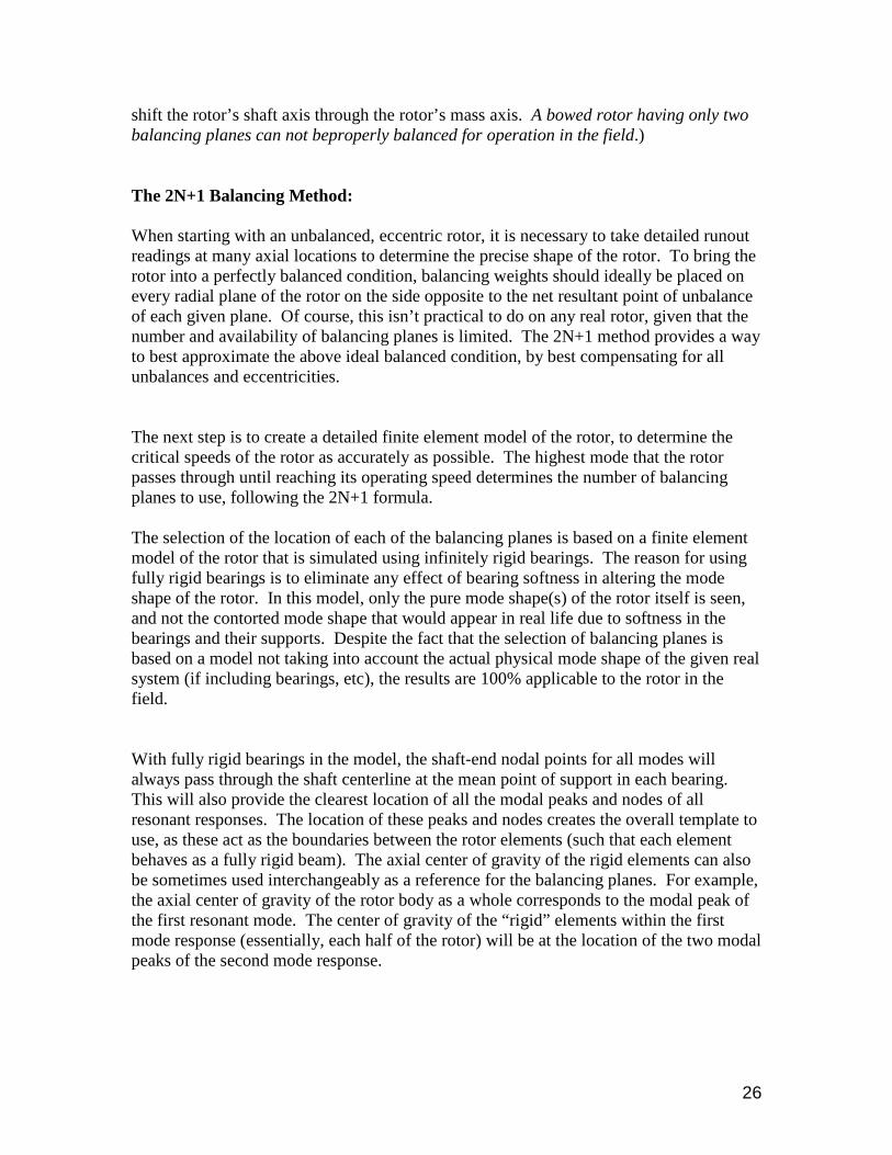
shift the rotor’s shaft axis through the rotor’s mass axis. A bowed rotor having only two balancing planes can not beproperly balanced for operation in the field.) The 2N+1 Balancing Method: When starting with an unbalanced, eccentric rotor, it is necessary to take detailed runout readings at many axial locations to determine the precise shape of the rotor. To bring the rotor into a perfectly balanced condition, balancing weights should ideally be placed on every radial plane of the rotor on the side opposite to the net resultant point of unbalance of each given plane. Of course, this isn’t practical to do on any real rotor, given that the number and availability of balancing planes is limited. The 2N+1 method provides a way to best approximate the above ideal balanced condition, by best compensating for all unbalances and eccentricities. The next step is to create a detailed finite element model of the rotor, to determine the critical speeds of the rotor as accurately as possible. The highest mode that the rotor passes through until reaching its operating speed determines the number of balancing planes to use, following the 2N+1 formula. The selection of the location of each of the balancing planes is based on a finite element model of the rotor that is simulated using infinitely rigid bearings. The reason for using fully rigid bearings is to eliminate any effect of bearing softness in altering the mode shape of the rotor. In this model, only the pure mode shape(s) of the rotor itself is seen, and not the contorted mode shape that would appear in real life due to softness in the bearings and their supports. Despite the fact that the selection of balancing planes is based on a model not taking into account the actual physical mode shape of the given real system (if including bearings, etc), the results are 100% applicable to the rotor in the field. With fully rigid bearings in the model, the shaft-end nodal points for all modes will always pass through the shaft centerline at the mean point of support in each bearing. This will also provide the clearest location of all the modal peaks and nodes of all resonant responses. The location of these peaks and nodes creates the overall template to use, as these act as the boundaries between the rotor elements (such that each element behaves as a fully rigid beam). The axial center of gravity of the rigid elements can also be sometimes used interchangeably as a reference for the balancing planes. For example, the axial center of gravity of the rotor body as a whole corresponds to the modal peak of the first resonant mode. The center of gravity of the “rigid” elements within the first mode response (essentially, each half of the rotor) will be at the location of the two modal peaks of the second mode response.

27

When selecting the elements for generating a FEA model, another rule of thumb is that the axial length of any element must not be any greater than the diameter of the element. In this way, it can be assured that each of the elements will behave independently as a purely rigid beam, and will have no bending within itself. QHSB-Method Example for a Rotor Operating Above its Third Critical Speed: The example showing the 2N+1 method is done on the same eccentric rotor model (with quasi-static distributed mass eccentricity) as for the other two methods above. Recall that the rotor operates above its third critical speed, and therefore, there will be seven balancing planes used. A summary diagram of the balancing planes, balancing shots and weight distributions used is shown in the Figure 8, and can be referenced during the explanation of the procedure. The five central, pre-selected balancing planes are those determined from FE modal analysis to be at the modal peaks and nodes of the first and second mode resonant responses. These planes, however, are used to resolve the rigid modes of the rotor resulting from the mass eccentricity. By successfully resolving the rigid modes, the first and second mode resonant mode responses will be eliminated as well.

28

Figure 8: Identification and location of balancing correction planes and weight distribution

29

The rigid lateral mode is balanced first, and uses the central three planes (planes 1, 2, and 3). The balance weights are placed in a proportional distribution where approximately half of the first static trial shot is placed at the midplane, and the other half is divided equally at each quarter-plane (the initial angle is based on the eccentricities indicated by the runout readings, or from an estimated phase lag observed on a Nyquist (Polar) plot. The reason for this distribution goes back to the concept that any fully rigid rotor can be balanced in two planes. Looking at the first mode response alone, each half of the rotor acts as a rigid beam, and therefore each half can be considered as a rigid element that can be balanced in two planes. Since each of these two rigid elements (with regard to the first mode) shares the midplane, this plane is essentially utilized twice, once for each rigid element. Since the first mode response is typically symmetric about the midplane, each of these two rigid elements will likely have a similar solution. Therefore, each rigid element receives the same initial solution in its balance shot, with the end result being that the midplane is used twice. The influence coefficients can then suggest an axial redistribution or phase shift of the weights to fine-tune the solution. The rocking rigid mode is then resolved similarly via a procedure of using trial shots and obtaining influence coefficients, using the outer two planes in pairs as 2 and 4 and 3 and 5, one set at a time. This distribution is refined using influence coefficients until it can be seen that there is no longer a rising upslope in the amplitude displayed on a Bode plot at speeds above the system first resonance. If there is a rising slope, then the rigid rocking mode has not been fully resolved (as can be observed later in Figure 12). This process ultimately results in five balancing planes being needed to fully solve the rigid mode responses from the eccentricity, which results in the rotor becoming dynamically straight. The rotor’s mass axis and shaft axis should be coincidental through the entire speed range, and no change in axis will occur above the first critical speed. If the rigid modes were solved correctly, then a Bode plot should show a flat horizontal line all the way to operating speed (with an amplitude value equal to the rotor’s eccentricity), with an exception possibly being a brief spike in amplitude at the second and third critical speeds (as can be seen later in Figure 14). If the amplitude has remained flat until a speed of 50% above the first critical, then it can be assured that it will remain flat for all higher speeds as well. This is the reason the term Quasi-High Speed can be used. There is not a need to run to the second critical speed or higher to continue balancing, as the solution is already completed. The only need is to run once to operating speed to verify if the third critical speed is being excited. The other two outboard balancing planes (planes 6 and 7) are used as part of standard modal weight configurations to resolve either the third critical (first flexural mode), or to resolve any additional response of the second resonant mode induced by the motion of long overhangs. If there is an increase in amplitude near the third critical speed, it can be seen if the responses at the ends of the rotor are in phase or out of phase, or possibly

30

some combination of both. If the responses are in phase, a modal V-shot should be used. If the responses are out of phase, a modal S-shot should be used. If the responses are a combination of both, the motion with larger amplitude should be balanced first with the appropriate modal shot, with refinement then done using the other modal shot. Lastly, in the rare occasion that a long overhang itself has an independent critical speed response, balancing weights in the couplings themselves can be used as part of a modal weight configuration. This last portion, though, is not considered to be a part of the overall 2N+1 balancing procedure, since any eccentricity of the overhangs MUST be resolved by machining before commencing any rotor balancing. Other Things to Remember: While balancing, if the position of the eccentricity can’t be measured directly, its true polar-angle direction can be determined based on the phase lag of the rotor’s displacement response at the first critical speed. The direction of the eccentricity will be 90 degrees ahead (in the direction of rotation) of the displacement response. Then, to balance the unbalance effect of eccentricity, the balance weights should be placed 180 degrees opposite to the eccentricity. This means that the weights to correct the rigid mode are placed 90 degrees behind the peak displacement response at the first critical. By balancing near the first system resonance, the clearest rotor response is seen, and the dynamic lag can be compensated based on the Polar plot data. If the response is being measured through force instead of displacement, then it should be remembered that force measured directly at low speeds doesn’t have phase lag, and the measurement will always point in the direction of the mass eccentricity. For speeds at the first critical and higher, the force may lag somewhat, depending on balancing speed and the system damping. This lag in directly measured force, however, is not the same as the lag in displacement, and the angle relation is determined by testing, i.e. the direction of eccentricity if based on force measurements alone at higher speeds can be better determined by obtaining influence coefficients. Additionally, when dealing with influence coefficients, the software calculation does not know that more than one plane is being used at a time for a given trial balance shot. Therefore, whatever results are obtained through influence coefficients must be applied proportionally to all the planes where weights were placed for that trial shot (each weight would adjusted up or down by the same percentage of its total mass). The Key Point Repeated: In summary, any rigid mode unbalance can be balanced in five planes (for a typical industrial rotor operating above its third critical speed). This method will solve the rigid lateral mode response (using the first three planes), and also solve the rigid rocking mode

31

response (using the additional two planes). The rotor balanced in this manner will be dynamically straight, and will not bend at any speed. Any higher mode resonant responses must be solved only with modal weight distributions so as not to disturb the rigid mode solution. More concisely still, the bending component of the vibration is to be resolved only with purely modal weights. The rigid component of the vibration is resolved as if dealing with a static beam, by simply compensating for all the distributed forces and the moments that are acting on the beam, by placing correction weights in axially preselected balancing planes. 2N+1 Method: Step by Step Example for a Real Generator Rotor: The following section shows plots for the balancing process of a real generator rotor, using the QHSB-Method (in 2N+1planes). The model results shown earlier were to simulate the balancing of this rotor (albeit using a “cleaner” eccentricity distribution – the real rotor had an eccentricity of around 2 mils, in a more randomly undefined distribution shape). Like in any balancing process, thoughtful planning must be done and predetermined rules must be followed. First Roll: The rotor is first rolled in its original unbalanced state to the maximum speed achievable, without exceeding preset vibration amplitude limits. An image of the Bode plot can be seen in Figure 9. In this example, the rotor’s run-up was halted upon observing an exponential increase in amplitude while approaching the first critical. If the speed were allowed to increase any further, the amplitude could potentially keep growing exponentially, risking bearing or rotor damage. To roll to higher speeds, a balance shot must be placed first. The rotor response is plotted using polar plots. This can show either displacements or velocities (which provide the forces), depending on the instrument setup of the balancing facility. The signals from sensors located at same reference angle from two journals are plotted on same polar plot. The polar plot for this first roll is seen in Figure 10. The amount of the first trial weight set is estimated using the 10% rule suggested by Bentley Nevada, which states that the centrifugal force generated from the trial weight, at operating speed should not exceed 10 percent of total rotor weight:

Wtrial = m * e * ω² = 0.1*Wrotor.

Based on the angles of the static response vectors at the highest speed reached (the vector arrows seen in Figure 10), with consideration of a possible phase lag, the first trial weight

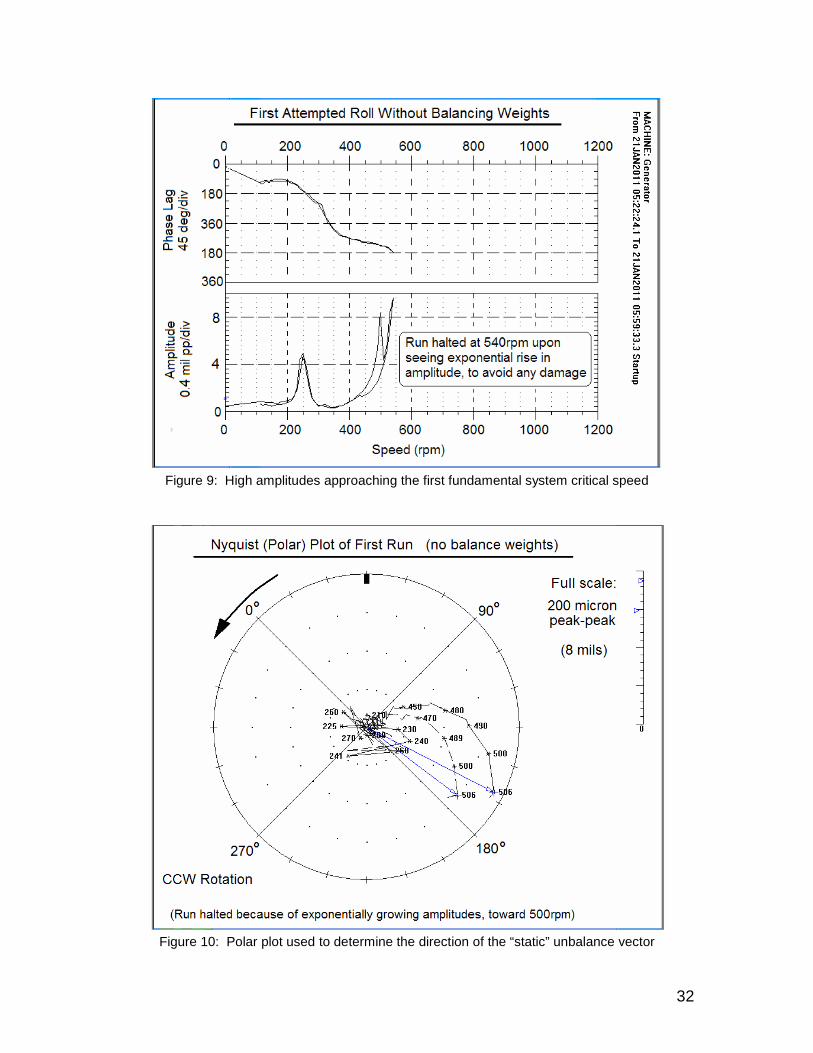
32

Figure 9: High amplitudes approaching the first fundamental system critical speed

Figure 10: Polar plot used to determine the direction of the “static” unbalance vector

33

set for the compensation of the rotor's rigid lateral mode (which excites the first system resonance) is distributed in three planes as shown earlier on Figure 8. The weight placement angle is chosen based on the direction of the response vector seen in the polar plot. The rotor is run again and the response is used to generate the first set of influence coefficients. Another run may be necessary to bring the amplitude of the rotor’s first system resonance down to the point where it is equal to the initial slow roll runout from eccentricity. The angle of the weights could be adjusted within +/- 5 degrees from the initial phase angle. The polar plot after placing the first trial shot is seen in Figure 11.

Figure 11: Trial shot placed in 3 planes, acting to resolve the amplitude at the first fundamental critical speed If the rotor amplitude rises at some slope after passing a resonance speed, it is an indication that the static unbalance is not symmetric (that is, the mass eccentricity is actually a quasi-static unbalance), and indicates that the true mass center is axially off by some distance from the rotor’s geometric center. This slope can be seen in the Bode plot in Figure 12.

34

Figure 12: Bode plot amplitude slope after critical speed; indication of CG off rotor’s geometric center

Figure 13: The rigid mode responses are resolved, continue to higher speeds

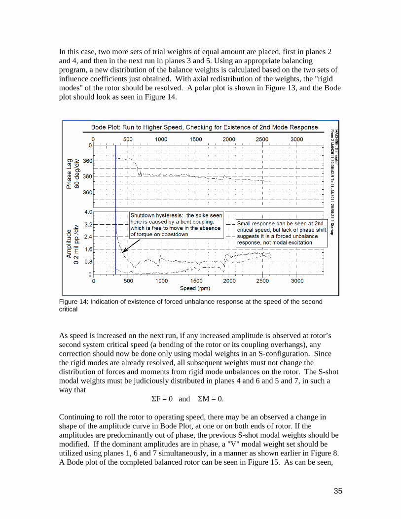
35

In this case, two more sets of trial weights of equal amount are placed, first in planes 2 and 4, and then in the next run in planes 3 and 5. Using an appropriate balancing program, a new distribution of the balance weights is calculated based on the two sets of influence coefficients just obtained. With axial redistribution of the weights, the "rigid modes" of the rotor should be resolved. A polar plot is shown in Figure 13, and the Bode plot should look as seen in Figure 14.

Figure 14: Indication of existence of forced unbalance response at the speed of the second critical As speed is increased on the next run, if any increased amplitude is observed at rotor’s second system critical speed (a bending of the rotor or its coupling overhangs), any correction should now be done only using modal weights in an S-configuration. Since the rigid modes are already resolved, all subsequent weights must not change the distribution of forces and moments from rigid mode unbalances on the rotor. The S-shot modal weights must be judiciously distributed in planes 4 and 6 and 5 and 7, in such a way that ΣF = 0 and ΣM = 0. Continuing to roll the rotor to operating speed, there may be an observed a change in shape of the amplitude curve in Bode Plot, at one or on both ends of rotor. If the amplitudes are predominantly out of phase, the previous S-shot modal weights should be modified. If the dominant amplitudes are in phase, a "V" modal weight set should be utilized using planes 1, 6 and 7 simultaneously, in a manner as shown earlier in Figure 8. A Bode plot of the completed balanced rotor can be seen in Figure 15. As can be seen,

36

the total vibration at the bearing locations at the end of the balancing process is less than half a mil through the entire speed range.

Figure 15: Final Bode plot of the sufficiently balanced rotor

If the final balancing weight distribution result were to be mapped out as a curve, it should ideally be a mirror image of the curve of the runout reading shape of the rotor. The Bode plot should remain a flat line for all speeds, and the rotor will be running dynamically straight. When a rotor is eccentric, the flat Bode plot line is not necessarily at zero, but may be flat at 1 or 2 mils which represents the amount of eccentricity in the rotor, and it cannot be reduced any farther. (Or rather, it could be “reduced” only by faking it, such as by actually unbalancing the rotor to an operating position where a nodal point is shifted to the displacement probe’s measuring location, which would dramatically increase the force of the rotor on the bearings.) It should be self evident that every possible combination of unbalance from eccentricities is impossible to predict. Nevertheless, by solving a rotor's rigid modes first, using the QHSB-Method with balancing plane selection based on the rotor's highest mode shape within its operating speed range, the rotor will be made "dynamically straight". By accomplishing this, the rotor will behave linearly through its entire operating speed range. With that, the effects of the inertia forces from any mass eccentricity, and any nonlinear rotor behavior can be avoided, making the entire balancing process simpler and more efficient. Excellent results can be obtained in fewer runs, and the end result is a well-balanced rotor that is guaranteed to run smoothly when installed in the field.

37

CONCLUSIONS: 1. Any rotor that is concentric within the limits of ISO 1940 regarding residual eccentricity can be successfully balanced using any of the balancing methods. 2. When using standard methods to balance any rotor that is bowed or eccentric, exceeding the criteria of ISO 1940, whether rigid or flexible, the rotor will be inadvertently balanced around its mass axis at speeds above the first system resonance. At operating speed, the rotor will be contorted and it will create or increase forces in the bearings if constrained by bearing clearances or by being coupled to other rotors. 3. All rigid, bowed rotors balanced by the N or the N+2 methods on a soft-bearing low speed balancing machine will be problematic after being coupled to other rotors and placed in service, if the final balance was completed while the rotor was spinning (or in precession) around its mass axis. 4. A rigid, eccentric rotor balanced using the N+2 method on a hard-bearing low speed balancing machine will be correctly balanced if it is balanced in three planes, and will operate fine after it is placed back in service. (Assuming the couplings are concentric to journals). 5. Any flexible, bowed or eccentric rotors operating above the second critical speed, and balanced by the N or the N+2 method will operate in a contorted shape, mimicking the highest operating mode shape. This condition can also create problems on composite rotors (generators) where some components can “lock up” and create vibrations from “thermal” related issues. 6. Any flexible or rigid rotors, with bows or eccentricities, balanced using the 2N+1, QHSB Method, after resolving the rotor’s rigid mode unbalances, will become dynamically straight, and will maintain its shape through all speeds. Even after using modal correction weights at higher speeds for fine-tuning if necessary, the rotor will operate as balanced around its shaft axis, with guaranteed performance in the field. 7. With many additional runs in a balancing facility and a lot of trial and error, a highly eccentric or bowed rotor may ultimately be brought to spin around its shaft axis and be balanced correctly using other methods as well. However, the number of runs, labor hours spent and the electricity costs for the drive motor used makes the choice of procedures an economics issue as well. 8. The QHSBM is applicable on any low or high speed balancing machine, saves the number of trial runs and uses less power during the balancing process. Finally, a rotor balanced by the Quasi-High Speed Balancing Method produces better balancing results, which makes follow-up balancing of the rotor in the field unnecessary.

38

Other Closing Comments: A Jeffcott rotor doesn’t fully represent the behavior of an eccentric rotor. In a Jeffcott model with a massless shaft holding an eccentric disk, the “rotor” can achieve a self-balanced state as the disk’s center of mass moves into the rotational axis at high speed. However, it accomplishes this in the model only by bending the shaft, and without the shaft transmitting any forces. In a real eccentric rotor, the entire shaft itself shifts the position of its rotational (or precessional) axes, and this dynamic motion both effects and depends on the transmission of forces into the bearings (and identifying this dynamic motion is the key to successful balancing). In the Jeffcott model, this dynamic behavior of the shaft itself and its resulting change in the forces on the bearings is generally neglected. The cross coupling (that is, the effect of the bearings on the rotor combined with the effect of the rotor on the bearings) between the static forces (bearing-originating) and dynamic forces (rotor-originating) is really an interaction between the inertia forces acting on the rotor and the dynamic stiffness acting at the bearings. The rotor’s static shaft centerline position is determined by the equilibrium of static forces in the bearings (as in a simple beam). The rotor’s dynamic motion or position (such as it’s varying precession of axes) is determined by the equilibrium of the forces from centripetal and tangential acceleration acting on every infinitesimal radial plane of any portion of the rotor in which there is mass eccentricity. Real-life rotors in a balancing bunker on two bearings can assume a self-balance state, with stable rotation centered around the mass axis. This can happen as long as the bearing clearances are larger than the rotor’s bow or mass eccentricity (tighter bearing clearances will restrain the rotor from shifting into its position of natural dynamic equilibrium). Real-life bowed rotors, or rotors with significant eccentricities can never achieve a self-balanced state when they are assembled in a rotor train, even when they were balanced “well” in a bunker by the N or N+2 methods.

The overall dynamic behavior described also applies to very high speed turbochargers, compressors, or vertical pumps with impellers mounted outboard of the bearings on a slender cantilever. They can seldom achieve their maximum designed operating speed, since eccentricity is introduced by shaft bending or by the impellers’ deformation or shaft-fits at very high speeds, usually at the system first critical speed. In these small rotors, if spinning at 50,000+ rpm, even a few microns of eccentricity can negatively impact its dynamic behavior.

Besides the standard rotor type classification by ANSI or ISO standards, rotors must be further classified between those being in compliance with ISO 1940 and those outside compliance, with regard to residual eccentricities.

39

If we balance only rotors that are in compliance, does that mean that those outside compliance cannot be balanced and that they should be discarded? NO! Rotors out of compliance must be further classified to those having eccentricities on the body between the axial centers of the journals, and those having eccentricities in sections outside of the body of the rotor (that is, outside the first mode nodal point or axial journal centerline), such as in the couplings, seals and journals.

Rotors with eccentricities of the body between the journal centers CAN be balanced using the appropriate number of balancing planes, proper plane locations and appropriate balancing method. Eccentricities of sections of the rotor outside the journal centers MUST be machined to bring the rotor into compliance. Rotors with significant eccentricities between the journals that do not have the sufficient number of balancing planes available cannot ever be properly balanced for operation in the field, before adding the necessary planes, or by corrective machining. Bibliography: 1 Bishop R.E.D. , Parkinson A.G., “On the Use of Balancing Machine for Flexible Rotors.”, Journal of

Engineering for Industry, pp 561-572, 1972

2 Kellenberger W.,” Should a Flexible Rotor be Balanced in N or N+2 Planes?” Transaction. ASME Journal of Engineering for Industry 94, No 2. 1972

3 Rieger N.F. and Zhou S. “Comparison of Effectiveness of Several Balancing Methods for Flexible Rotors.” Proceedings of IFToMM Conference on Rotordynamic Applications in Power Plants, Rome Italy, 1982.

4 Gunter E.J. Dynamic Stability of Rotor Bearing Systems, Washington DC: NASA report SP-113, 1966.

5 Gunter E.J, Barrett L.E., Allaire P.E. “Balancing of Multimass Flexible Rotors, Part I: Theory and Part II: Experimental Results.” Proceedings of the Fifth Turbomachinery Symposium, Texas A&M, October 1976.

6 Ehrich F. Handbook of Rotordynamics, McGraw-Hill, 1992.

7 Bently D.E., Hatch C.T., and Grissom B. Fundamental of Rotating Machinery Diagnostics, Bently Pressurized Bearing Press, Minden NV, 2002.

8 Racic Z. and Hidalgo J. “Practical Balance of Flexible Rotors for Power Generation.” Proceedings of the ASME IDETC/CIE Conference, Las Vegas NV, USA, September 2007

9 Racic Z. and Hidalgo J. “The Effect of Applied High Speed Balancing Method on Flexible Generator Rotor Response in Operation.” Proceedings of the ISCORMA-4, Calgary, Canada, August 2007

10 Rao S.S., Engineering Optimization, Theory and Practice. 3rd Edition NY, Willey-Interscience, 1996 11 Ferdinand P. Beer and E. Russell Johnston Jr. Sixth Edition, Vector Mechanics for Engineers – Dynamics, WCB, McGraw- Hill, 1997. 12 Victor Wowk, Machinery Vibrations: Balancing, A McGraw-Hill, Special Reprint Edition, 1995. 13 Mark S. Darlow, Balancing of High Speed Machinery, Springer-Verlag, 1989.

40

14 Robert G. Loewy, Vincent J. Piarulli, Rochester Applied Science Associates, Inc., Internal, 1969. 15 Hato Schneider, Balancing Technology, Schenck, 1991.