Rosa Ramirez ( Université d’Evry ) Shuangliang Zhao ( ENS Paris) Classical Density Functional...
42
• Rosa Ramirez (Université d’Evry) • Shuangliang Zhao (ENS Paris) sical Density Functional Theory of Solvation in Molecular Sol Daniel Borgis Département de Chimie Ecole Normale Supérieure de Paris [email protected]
-
Upload
esther-gregory -
Category
Documents
-
view
222 -
download
2
Transcript of Rosa Ramirez ( Université d’Evry ) Shuangliang Zhao ( ENS Paris) Classical Density Functional...

• Rosa Ramirez (Université d’Evry)• Shuangliang Zhao (ENS Paris)
Classical Density Functional Theory of Solvation in Molecular Solvents
Daniel Borgis Département de Chimie
Ecole Normale Supérieure de [email protected]

Solvation: Some issues
For a given molecule in a given solvent, can we predict efficiently and with « chemical accuracy:
• The solvation free energy
• The microscopic solvation profile
A few applications:• Differential solvation (liquid-liquid extraction)• Solubility prediction• Reactivity• Biomolecular solvation, ….
Explicit solvent/FEP

Solvation: Implicit solvent methods
Dielectric continuum approximation (Poisson-Boltzmann)
rrr 04 r
i
80
Biomolecular modelling: PB-SA method
AdF rrr 02
1
Solvent Accessible Surface Area (SASA)
electrostatics + non-polar
Quantum chemistry: PCM method

Improved implicit solvent models
• Integral equations
• Interaction site picture (RISM) (D. Chandler, P. Rossky, M. Pettit, F. Hirata, A. Kovalenko)
• Molecular picture (G. Patey, P. Fries, …)
• Classical Density Functional Theory
This work: Can we use classical DFT to define an improved and well-founded implicit solvation approach?
(based on « modern » liquid state theory)
)(, rcrh ijijSite-site OZ + closure
Molecular OZ + closure 21122112 ,,,,, ΩΩrΩΩr ch

)'()'()('2
1)()(
1)(
4
2
1)( 0
2 rPrrTrPrrrErPrPr
rrP
dddrdF
Fpol
entropy
Fexc
Solvent-solvent
Fext
P(r)
ir
]);([)(0 iielec FVU rrPr
DFT formulation of electrostatics

Dielectric Continuum Molecular Dynamics
M. Marchi, DB, et al., J. Chem Phys. (2001), Comp. Phys. Comm. (2003)
Use analogy with electronic DFT calculations and CPMD method
k
rkkPrP )exp()()( i
ii
ii
P
VF
dt
dm
F
dt
dM
rr
r
kP
kP
02
2
2
2
)(
)(
On-the-fly minimization with extended Lagrangian
Plane wave expansion
Soft « pseudo-potentials »
)(1111
rr
Hsis

Dielectric Continuum Molecular Dynamics
-helix horse-shoe

Dielectric Continuum Molecular Dynamics
Energy conservation Adiabaticity

Beyond continuum electrostatics: Classical DFT of solvation
densitysolventnorientatioposition/, Ωr
In the grand canonical ensemble, the grandpotential can be written as a functional of (r
NVddFST cextexc ΩrΩrΩr ,,
0
Ωr,0
Ωr,0Functional minimization:
Thermodynamic equilibriumD. Mermin (« Thermal properties of the inhomogeneous electron gas », Phys. Rev., 137 (1965))
Intrinsic to a given solvent

In analogy to electronic DFT, how to use classical DFT as a « theoretical chemist »tool to compute the solvation properties of molecules, in particular their solvationfree-energy ?
0 Ωr,
0 F
energy freeSolvation min F
0, c ),(, Ωrextc V
But what is the functional ??

The exact functional
extexcid FFFF x
01
0
111 ln
xxxx
dTkF Bid
111 xxx extext VdF
,, 121121 xxxxxx CddTkF Bexc 0 xx
;,1, 21)2(1
021 xxxx cdC xx 0
),( Ωrx
),( Ωr

The homogeneous reference fluid approximation
Neglect the dependence of c(2)(x1,x2,[]) on the parameter , i.e use
direct correlation function of the homogeneous system
21021)2(
21)2( ,;,;, xxxxxx ccc
c(x1,x2) connected to the pair correlation function h(x1,x2) through the Ornstein-Zernike relation
2331302121 ,,,, xxxxxxxxx hcdch
1,, 2121 xxxx ghg(r)
h(r)

The homogeneous reference fluid approximation
Neglect the dependence of c(2)(x1,x2,[]) on the parameter , i.e use
direct correlation function of the homogeneous system
21021)2(
21)2( ,;,;, xxxxxx ccc
c(x1,x2) connected to the pair correlation function h(x1,x2) through the Ornstein-Zernike relation
2332311333021122112 ,,),,(,,,, ΩΩrΩΩrΩrΩΩrΩΩr hcddch
1,, 2121 xxxx ghg(r)
h(r)

),,(h 2112 ΩΩr
),,(c 2112 ΩΩr
The picture
Functional minimization

Rotational invariants expansion
),,ˆ(),,( 2112122112 ΩΩrΩΩr lmnlmn rhh
),,ˆ(),,( 2112122112 ΩΩrΩΩr lmnlmn rcc
1Ω
2Ω
12r

21121121112
21110000 ))((3,,1 ΩΩrΩrΩΩΩ
The case of dipolar solvents
The Stockmayer solvent
1Ω
2Ω
12r
11212
11211012
11000012
0002112 )()()(),,( rcrcrcc ΩΩr

Particle density Polarization density
ΩrΩr , dn ΩrΩΩrP ,0 d
Ωr,F rPr ,nF
densitysolventnorientatioposition/, Ωr
R. Ramirez et al, Phys. Rev E, 66, 2002 J. Phys. Chem. B 114, 2005
A generic functional for dipolar solvents

A generic functional for dipolar solvents
PPPP ,,,, nFnFnFnF excextid
010
111 )(
)(ln)(, nn
n
nndTknF Bid
r
rrrP
)(/)(L)(
)(/)(Lsinh
)(/)(Lln 0
1
01
01
rrrrr
rrr nPP
nP
nPdTkB
)()( rPr P
L(x)LangevindefonctionladeInverse)(L 1 x

A generic functional for dipolar solvents
PPPP ,,,, nFnFnFnF excextid
010
111 )(
)(ln)(, nn
n
nndTknF Bid
r
rrrP
)(2
)( 2
r
rPr
ndTk
dB
litypolarizabinalorientatiolocal3
2
TkB
d

A generic functional for dipolar solvents
PPPP ,,,, nFnFnFnF excextid
)()()()(, rPrrrrrP qLJext EdnVdnF

A generic functional for dipolar solvents
PPPP ,,,, nFnFnFnF excextid
)()()(2
, 212000
121 rrrrP nrcnddTk
nF Bexc
)()()()(3)(2 2112212112
11221
rPrPrrPrrPrr rcddTkB
)()()(2 2112
11021 rPrPrr rcdd
TkB
Connection to electrostatics: R. Ramirez et al, JPC B 114, 2005

)(
)(
)(
12112
12110
12000
rh
rh
rh
The picture
Functional minimization
)(
)(
)(
12112
12110
12000
rc
rc
rc

O-Z
h-functions c-functions
Step 1: Extracting the c-functions from MD simulations
Pure Stockmayer solvent, 3000 particles, few ns
= 3 A, n0 = 0.03 atoms/A3 0 = 1.85 D, = 80

Step 2: Functional minimisation around a solvated molecule
• Minimization with respect to • Discretization on a cubic grid (typically 643)• Conjugate gradients technique• Non-local interactions evaluated in Fourier space (8 FFts per minimization step)
)(and)( rPrn
Minimisation step

N-methylacetamide: Particle and polarization densities
trans cis

N-methylacetamide: Radial distribution functions
H
CH3
O
N
C

N-methylacetamide: Isomerization free-energy
cis trans
Umbrella sampling
DFT

DFT: General formulation
One needs higher spherical invariants expansions or angular grids
2112 ,,cand, ΩΩrΩrTo represent:
4N 8N
32 NNN
Begin with a linear model ofAcetonitrile (Edwards et al)
(with Shuangliang Zhao)

Step 1: Inversion of Ornstein-Zernike equation
2331302121 ,,,,,,,, ΩΩkΩΩkΩΩΩkΩΩk hcdch
10 ))()(()( kHWIkHkC
Step 2: Minimization of the discretized functional
extexcid FFFF x
0
0
ln
Ωr,Ωr,
Ωr,ΩrddTkF Bid
Ωr,Ωr,Ωr extext VddF
222121221111 ),,(2
1Ω,rΩΩrrΩrΩ,rΩr cddddFexc
Vexc(r1,1)

Step 2: Minimization of the discretized functional
• Discretization of on a cubic grid for positions and Gauss-Legendre grid for orientations (typically 643 x 32)
2,, ΩrΩr
• Minimization in direct space by quasi-Newton (BFGS-L) (8x10⁶ variables !!)
• 2 x N = 64 FFTs per minimization step
~20 s per minimization step on a single processor
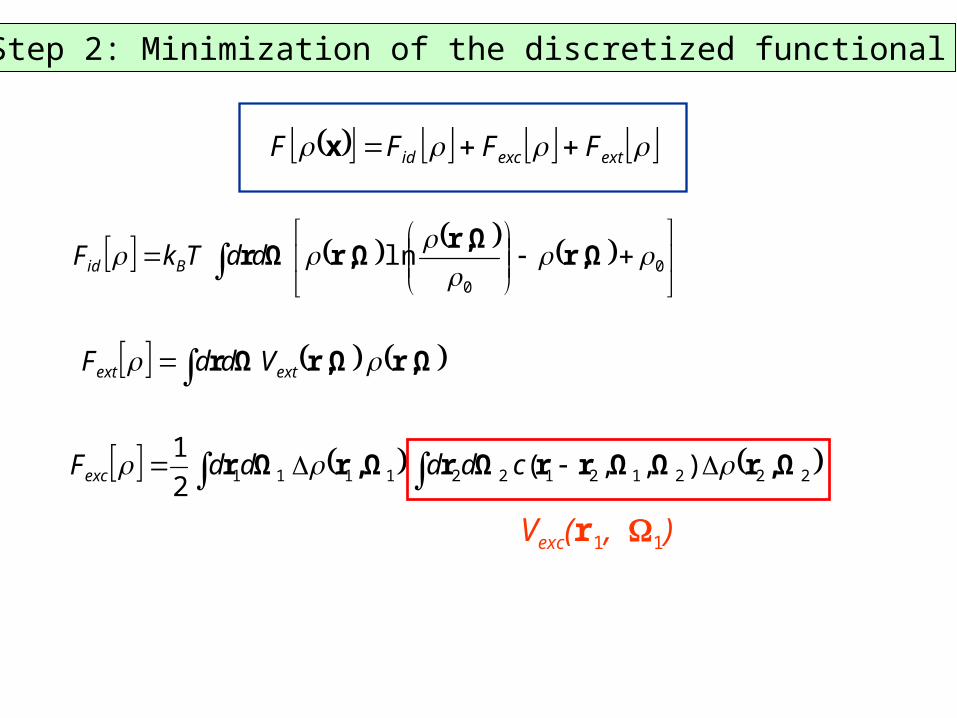
MD
DFT
Solvent structure
Na+Na
Solvation in acetonitrile: Results
MD
DFT

Solvation in acetonitrile: Results
MD (~20 hours)
DFT (10 mn)

Solvation in acetonitrile: Results
Halides solvation free energy
Parameters for ion/TIP3P interactions

Solvation in SPC/E water
Solute-Oxygen radial distribution functions
MD
DFT
Z
X
Y
Three angles: ,,

CH3
C
N
Solvation in SPC/E water

Cl-q
Solvation in SPC/E water

Solvation in SPC/E water
Water in water
HNC PL-HNC HNC+B
g OO(r
)

Conclusion DFT
• One can compute solvation free energies and microscopic solvation profiles using « classical » DFT
• Solute dynamics can be described using CPMD-like techniques
• For dipolar solvents, we presented a generic functional of or
• Direct correlation functions can be computed from MD simulations • For general solvents, one can use angular grids instead of rotational invariants expansion
rP
• BEYOND: -- Ionic solutions -- Solvent mixtures -- Biomolecule solvation
rPr ,n
R. Ramirez et al, Phys. Rev E, 66, 2002 J. Phys. Chem. B 114, 2005 Chem. Phys. 2005L. Gendre at al, Chem. Phys. Lett.S. Zhao et al, In prep.

DCMD: « Soft pseudo-potentials »
V(r)
r
V(r) = (r)-1= 4/((r)-1)
V(r)
r
)(1111
rr
Hsis
=0

Dielectric Continuum Molecular Dynamics
Hexadecapeptide P2
La3+ Ca2+

DCMD: Computation times
System Nb of atoms
CPU total
CPU forces
CPU TIP3P
Dipep-tide
22 3.2 0.1 2.45
Octa 83 3.3 0.3 2.45
BPTI 892 5.7 2.7 2.72
Each time step correspond to a solvent free energy, thus an average over many solvent microscopic configurations
linear in N !