
ROS Based High Performance Control Architecture for an ...
114
University of New Mexico UNM Digital Repository Electrical and Computer Engineering ETDs Engineering ETDs Fall 7-31-2017 ROS Based High Performance Control Architecture for an Aerial Robotic Testbed Christoph Hintz University of New Mexico Follow this and additional works at: hps://digitalrepository.unm.edu/ece_etds Part of the Controls and Control eory Commons is esis is brought to you for free and open access by the Engineering ETDs at UNM Digital Repository. It has been accepted for inclusion in Electrical and Computer Engineering ETDs by an authorized administrator of UNM Digital Repository. For more information, please contact [email protected]. Recommended Citation Hintz, Christoph. "ROS Based High Performance Control Architecture for an Aerial Robotic Testbed." (2017). hps://digitalrepository.unm.edu/ece_etds/389
Transcript of ROS Based High Performance Control Architecture for an ...

University of New MexicoUNM Digital Repository
Electrical and Computer Engineering ETDs Engineering ETDs
Fall 7-31-2017
ROS Based High Performance ControlArchitecture for an Aerial Robotic TestbedChristoph HintzUniversity of New Mexico
Follow this and additional works at: https://digitalrepository.unm.edu/ece_etds
Part of the Controls and Control Theory Commons
This Thesis is brought to you for free and open access by the Engineering ETDs at UNM Digital Repository. It has been accepted for inclusion inElectrical and Computer Engineering ETDs by an authorized administrator of UNM Digital Repository. For more information, please [email protected].
Recommended CitationHintz, Christoph. "ROS Based High Performance Control Architecture for an Aerial Robotic Testbed." (2017).https://digitalrepository.unm.edu/ece_etds/389

Candidate Department This thesis is approved, and it is acceptable in quality and form for publication: Approved by the Thesis Committee: , Chairperson

ROS Based High Performance ControlArchitecture for an Aerial Robotic
Testbed
by
Christoph Hintz
B.S., in Mechanical Engineering, Texas A&M University - Corpus
Christi, 2015
THESIS
Submitted in Partial Fulfillment of the
Requirements for the Degree of
Master of Science
Electrical Engineering
The University of New Mexico
Albuquerque, New Mexico
December, 2017

Dedication
To my parents, Grit and Mario, as well as my partner, Jasmine, for their support
and encouragement they gave me along the way. Dankeschon fur eure Hilfe.
“If something hasn’t broken on your helicopter, it’s about to.” – from ”Introduction
to Helicopter and Tiltrotor Flight Simulation” by Mark E. Dreier
iii

Acknowledgments
I would like to thank my grandparents, Erika and Gunter Hoppe, my siblings,Marieke and Lene Hintz, as well as my closest friend Philipp Bahr, who encouragedand supported me throughout the process.
I would like to thank my academic advisor, Professor Rafael Fierro to give me theability to do research with him, as well as supporting and advising me throughoutthe process. Additionally, I would like to thank Professor Francesco Sorrentino andProfessor Svetlana Poroseva for their advice and being a part of my committee.
Lastly, I want to thank all the MARHES friends and members for their helpduring the process. I would like to name Patricio Cruz, Gregory Brunson, StevenMaurice, Shakeeb Ahmad, Corbin Wilhelmi and Joseph Kloeppel for their help andadvice throughout this process.
iv

ROS Based High Performance ControlArchitecture for an Aerial Robotic
Testbed
by
Christoph Hintz
B.S., in Mechanical Engineering, Texas A&M University - Corpus
Christi, 2015
M.S., Electrical Engineering, University of New Mexico, 2017
Abstract
The purpose of this thesis is to show the development of an aerial testbed based
on the Robot Operating System (ROS). Such a testbed provides flexibility to control
heterogenous vehicles, since the robots are able to simply communication with each
other on the High Level (HL) control side. ROS runs on an embedded computer
on-board each quadrotor. This eliminates the need of a Ground Base Station, since
the complete HL control runs on-board the Unmanned Aerial Vehicle (UAV).
The architecture of the system is explained throughout the thesis with detailed
explanations of the specific hardware and software used for the system. The imple-
mentation on two different quadrotor models is documented and shows that even
though they have different components, they can be controlled similarly by the
framework. The user is able to control every unit of the testbed with position,
velocity and/or acceleration data. To show this independency, control architectures
are shown and implemented. Extensive tests verify their effectiveness. The flexibility
v

of the proposed aerial testbed is demonstrated by implementing several applications
that require high-performance control.
Additionally, a framework for a flying inverted pendulum on a quadrotor using
robust hybrid control is presented. The goal is to have a universal controller which
is able to swing-up and balance an off-centered pendulum that is attached to the
UAV linearly and rotationally. The complete dynamic model is derived and a con-
trol strategy is presented. The performance of the controller is demonstrated using
realistic simulation studies. The realization in the testbed is documented with mod-
ifications that were made to the quadrotor to attach the pendulum. First flight tests
are conducted and are presented.
The possibilities of using a ROS based framework is shown at every step. It has
many advantages for implementation purposes, especially in a heterogeneous robotic
environment with many agents. Real-time data of the robot is provided by ROS
topics and can be used at any point in the system. The control architecture has been
validated and verified with different practical tests, which also allowed improving the
system by tuning the specific control parameters.
vi

Contents
List of Figures xi
List of Tables xvi
Glossary xvii
1 Introduction 1
1.1 Motivation . . . . . . . . . . . . . . . . . . . . . . . . . . . . . . . . . 1
1.2 Problem Statement . . . . . . . . . . . . . . . . . . . . . . . . . . . . 3
1.3 Related Work . . . . . . . . . . . . . . . . . . . . . . . . . . . . . . . 4
1.4 Organization of this Thesis . . . . . . . . . . . . . . . . . . . . . . . . 6
2 System Overview 7
2.1 Hardware . . . . . . . . . . . . . . . . . . . . . . . . . . . . . . . . . 7
2.1.1 MARHES Testbed . . . . . . . . . . . . . . . . . . . . . . . . 7
2.1.2 AscTec Hummingbird . . . . . . . . . . . . . . . . . . . . . . . 8
vii

Contents
2.1.3 QAV250 . . . . . . . . . . . . . . . . . . . . . . . . . . . . . . 10
2.1.4 Vicon System . . . . . . . . . . . . . . . . . . . . . . . . . . . 12
2.1.5 Odroid XU4 . . . . . . . . . . . . . . . . . . . . . . . . . . . . 14
2.2 Software . . . . . . . . . . . . . . . . . . . . . . . . . . . . . . . . . . 16
2.2.1 ROS . . . . . . . . . . . . . . . . . . . . . . . . . . . . . . . . 16
3 Modeling of the Quadrotor 21
3.1 Kinematics Model . . . . . . . . . . . . . . . . . . . . . . . . . . . . . 21
3.2 Dynamic Model of a Quadrotor . . . . . . . . . . . . . . . . . . . . . 23
3.2.1 Newton-Euler Approach . . . . . . . . . . . . . . . . . . . . . 26
3.2.2 Linearized Model . . . . . . . . . . . . . . . . . . . . . . . . . 29
3.3 System Architecture . . . . . . . . . . . . . . . . . . . . . . . . . . . 32
4 Applications 34
4.1 MAST . . . . . . . . . . . . . . . . . . . . . . . . . . . . . . . . . . . 34
4.1.1 Introduction . . . . . . . . . . . . . . . . . . . . . . . . . . . . 34
4.1.2 Architecture . . . . . . . . . . . . . . . . . . . . . . . . . . . . 35
4.1.3 Velocity Estimator . . . . . . . . . . . . . . . . . . . . . . . . 38
4.1.4 Demo . . . . . . . . . . . . . . . . . . . . . . . . . . . . . . . 41
4.2 ASAP . . . . . . . . . . . . . . . . . . . . . . . . . . . . . . . . . . . 42
4.2.1 Introduction . . . . . . . . . . . . . . . . . . . . . . . . . . . . 42
viii
Contents
4.3 System Schematic . . . . . . . . . . . . . . . . . . . . . . . . . . . . . 43
4.4 Trajectory Tracking . . . . . . . . . . . . . . . . . . . . . . . . . . . . 44
4.5 Experimental Results . . . . . . . . . . . . . . . . . . . . . . . . . . . 45
5 Inverted Pendulum on a Quadrotor 48
5.1 Model . . . . . . . . . . . . . . . . . . . . . . . . . . . . . . . . . . . 49
5.2 Control Design . . . . . . . . . . . . . . . . . . . . . . . . . . . . . . 54
5.2.1 Energy Control . . . . . . . . . . . . . . . . . . . . . . . . . . 55
5.2.2 LQR Control . . . . . . . . . . . . . . . . . . . . . . . . . . . 56
5.3 Stability Analysis . . . . . . . . . . . . . . . . . . . . . . . . . . . . . 59
5.4 Matlab . . . . . . . . . . . . . . . . . . . . . . . . . . . . . . . . . . . 60
5.4.1 Linear Pendulum . . . . . . . . . . . . . . . . . . . . . . . . . 61
5.4.2 Rotational Pendulum . . . . . . . . . . . . . . . . . . . . . . . 62
5.4.3 Reduce Swinging . . . . . . . . . . . . . . . . . . . . . . . . . 64
5.5 Gazebo . . . . . . . . . . . . . . . . . . . . . . . . . . . . . . . . . . . 65
5.6 Implementation . . . . . . . . . . . . . . . . . . . . . . . . . . . . . . 69
6 Conclusions, Contributions and Improvements 74
6.1 Conclusions . . . . . . . . . . . . . . . . . . . . . . . . . . . . . . . . 74
6.2 Contributions . . . . . . . . . . . . . . . . . . . . . . . . . . . . . . . 75
6.3 Improvements . . . . . . . . . . . . . . . . . . . . . . . . . . . . . . . 76
ix

Contents
Appendices 78
A Graphs for Trajectory Tracking a Figure Eight 79
B Gazebo Simulation 84
C Picture Sequence of Gazebo Simulation 86
References 89
x

List of Figures
1.1 Drawing of the MARHES testbed with quadrotors in the Vicon mo-
tion capture area. The UAV in the front is able to go out of the
Vicon area by getting position information from a camera. . . . . . . 3
2.1 Heterogenous MARHES Testbed with a variety of humanoid, ground
and aerial robots in the Vicon motion capture area. . . . . . . . . . 8
2.2 AscTec Hummingbird quadrotor with Odroid XU4 microprocessor
on top of it and Vicon markers attached. . . . . . . . . . . . . . . . 9
2.3 QAV250 frame based quadrotor with Odroid XU4 microprocessor on
top of it and Vicon markers attached. The Odroid is secured by a
custom design and 3D printed part. . . . . . . . . . . . . . . . . . . 11
2.4 Schematic of the Vicon system and its setup in the laboratory. . . . 13
2.5 Vicon equipment for setup and view of Tracker software. . . . . . . . 14
2.6 Odroid XU4 microprocessor from Hardkernel. . . . . . . . . . . . . . 15
2.7 Publish/Subscribe concept of topics by nodes in the Robotic Oper-
ating System [1] . . . . . . . . . . . . . . . . . . . . . . . . . . . . . 17
xi

List of Figures
3.1 Schematic diagram of the quadrotor aerial vehicle. The world frame
A shown in black and the body frame B shown in green with
their related axes. The distance from the origin of the world frame
to the origin of the body frame is shown by r in red. The system
characteristics are symbolized in light blue. . . . . . . . . . . . . . . 22
3.2 Overview of the closed loop control architecture implemented and
parts where the different controllers are running. . . . . . . . . . . . 32
4.1 Heterogeneous robot system consisting of aerial and ground units.
Cloud resources to optimize the mission. . . . . . . . . . . . . . . . . 36
4.2 Control schematic for waypoint following of AscTec Hummingbird.
The asctec mav framework controllers are bypassed and only used
to send angles and thrust references to the LL attitude controller. . 37
4.3 Waypoint following results for AscTec Hummingbird on-board build
in controller vs. custom linear controller. . . . . . . . . . . . . . . . 38
4.4 Waypoint following results for AscTec Hummingbird on-board build
in controller vs. custom linear controller. . . . . . . . . . . . . . . . 39
4.5 Comparison of the velocity estimator algorithms explained. . . . . . 40
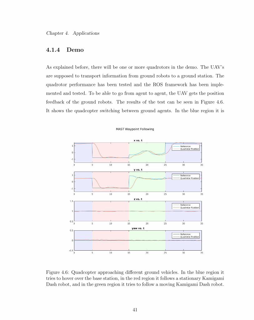
4.6 Quadcopter approaching different ground vehicles. In the blue region
it tries to hover over the base station, in the red region it follows a
stationary Kamigami Dash robot, and in the green region it tries to
follow a moving Kamigami Dash robot. . . . . . . . . . . . . . . . . 41
4.7 ASAP project. The idea of vehicle detection, tracking and neutral-
ization. . . . . . . . . . . . . . . . . . . . . . . . . . . . . . . . . . . 43
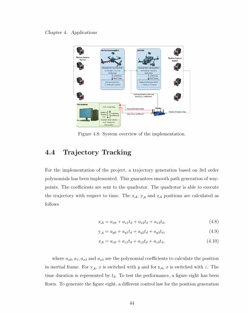
4.8 System overview of the implementation. . . . . . . . . . . . . . . . . 44
xii

List of Figures
4.9 x vs. y graphs of figure eight trajectory tracking at different speeds . 46
4.10 Experimental results of Scenario 1 for the implementation of the
reachability analysis . . . . . . . . . . . . . . . . . . . . . . . . . . . 47
4.11 Experimental results of Scenarios 2 for the implementation of the
reachability analysis . . . . . . . . . . . . . . . . . . . . . . . . . . . 47
5.1 Schematic diagram of the quadrotor with the pendulum (red), pen-
dulum arm extension (Yellow) and counterweight (blue) attached to
it. The world frame A shown in gray and the body frame B
shown in green with their related axes. The distance from the origin
of the world frame to the origin of the body frame is shown in red.
The system characteristics are symbolized in light blue. . . . . . . . 49
5.2 Block Diagram of the Control Schematic . . . . . . . . . . . . . . . 54
5.3 Stability analysis of the hybrid controller. . . . . . . . . . . . . . . . 60
5.4 Responses of the states to balance the pendulum with LQR control.
First graph shows the y position of the quadrotor, second graph
shows the pitch angle of the quadrotor and the last graph shows the
pendulum angle. . . . . . . . . . . . . . . . . . . . . . . . . . . . . . 62
5.5 Responses of the states to balance the pendulum with heading change
of the quadrotor. First graph shows the heading angle yaw of the
quadrotor and the last graph shows the pendulum angle. . . . . . . 63
5.6 Responses of the states to reducing the swing of the pendulum. First
graph shows the y position of the quadrotor, second graph shows the
pitch angle of the quadrotor and the last graph shows the pendulum
angle. . . . . . . . . . . . . . . . . . . . . . . . . . . . . . . . . . . . 65
xiii

List of Figures
5.7 Translational position and rotational angle of quadrotor and pendu-
lum for linear swing-up and balancing. . . . . . . . . . . . . . . . . . 67
5.8 Translational position and rotational angle of quadrotor and pendu-
lum for rotational swing-up and balancing. . . . . . . . . . . . . . . 68
5.9 Quadcopter with attached pendulum. Custom designed and printed
parts to cover Odroid XU4, hold markers, attach the pendulum to
quadrotor and attach pendulum to ball bearing. . . . . . . . . . . . 70
5.10 Linear position control of quadrotor with pendulum attached. . . . . 71
5.11 Rotational position control of quadrotor with pendulum attached. . 72
A.1 Position vs. time graphs for trajectory tracking figure eight with gain
k=0.5 . . . . . . . . . . . . . . . . . . . . . . . . . . . . . . . . . . . 80
A.2 Position vs. time graphs for trajectory tracking figure eight with gain
k=1.0 . . . . . . . . . . . . . . . . . . . . . . . . . . . . . . . . . . . 81
A.3 Position vs. time graphs for trajectory tracking figure eight with gain
k=1.5 . . . . . . . . . . . . . . . . . . . . . . . . . . . . . . . . . . . 82
A.4 Position vs. time graphs for trajectory tracking figure eight with gain
k=2.0 . . . . . . . . . . . . . . . . . . . . . . . . . . . . . . . . . . . 83
B.1 Control tree of Gazebo simulation with all control nodes and used
topics. . . . . . . . . . . . . . . . . . . . . . . . . . . . . . . . . . . 85
C.1 Picture sequence of swing-up and balancing simulation the linear
pendulum on a quadrotor in Gazebo. . . . . . . . . . . . . . . . . . 87
xiv

List of Figures
C.2 Picture sequence of swing-up and balancing simulation the rotational
pendulum on a quadrotor in Gazebo. . . . . . . . . . . . . . . . . . 88
xv

List of Tables
2.1 ROS Distributions since December 31, 2012. Additionally, informa-
tion about the compatibility with Ubuntu versions and end of date
for their support. . . . . . . . . . . . . . . . . . . . . . . . . . . . . 18
xvi

Glossary
A World frame
B Body frame
r Distance between world and body frame
ARB Orientation of body frame with respect to the world frame
xA, yA and zA Position of quadrotor origin in world frame
φ, θ and ψ Quadrotor Euler angles in world frame
xB, yB and zB Position of quadrotor origin in body frame
p, q and r Rotational angles in body frame
T1, T2, T3 and T4 Thrust of each of the four motors
Lq Distance between quadrotor origin and motor
ξ Position vector of quadrotor in inertial frame
η Attitude vector of quadrotor in inertial frame
q Vector containing linear and angular position of quadrotor in inertial
frame
xvii

Glossary
vA Linear velocity vector in inertial frame
ν Angular velocity vector in body frame
I Inertia matrix
Ixx, Iyy and Izz Inertia’s around xB, yB and zB, respectively
Tf Collective thrust from the four rotors
τxB , τyB , τzB Moment created by motors around xB, yB and zB, respectively
ρ Air density
Ct Aerodynamic coefficient
Cd Moment coefficient of the blade
rb Blade radius
ω Rotational speed of propeller
kt Force constant
km Moment constant
Mi Moment created by i-th motor
MB Moment matrix including the moments acting on the quadrotor
u Control matrix
mq Mass of the quadrotor
f Non-conservative forces applied to the quadrotor
Ω Skew-symmetric matrix
xviii

Glossary
g Earth gravity constant
Kp, Ki and Kd Tunable proportional, integral and derivative control gains, respec-
tively
e Error between desired and actual value
vx Velocity of x
Ts Sampling time
ax0, ax1, ax2 and ax3 Polynomial coefficients for x
k Gain for trajectory tracking speed
xL Position vector of pendulum
ω Angular velocity in body frame
Le Distance from quadrotor origin to pendulum pivot
Lp Pendulum length
S− Suspension point reference frame
S+ Reference frame always parallel to B
T Kinetic Energy
Vp Potential Energy
Ip Pendulum Inertia
L Lagrangian
α Pendulum angle
E Energy
xix

Glossary
J Quadratic cost function
K Control matrix
Q Performance index matrix
R State cost matrix
V1 and V2 Lyapunov function candidates
xx

Chapter 1
Introduction
1.1 Motivation
Unmanned aerial vehicles are becoming more popular, due to their capabilities.
There is an infinite amount of possibilities where these semi-autonomous or fully-
autonomous systems can assist humans to reduce time, improve quality or decrease
danger. Possible applications are search and rescue, delivery, environmental moni-
toring, photography, etc. As they become more advanced and less expensive they
also emerge into the educational sector, especially as control examples.
The quadrotor is one of the more popular unmanned aerial vehicles, due to its
vertical take-off and landing capabilities, hovering flight and simple control. As a
result many research groups use them as part of their testbed [2–5]. Its model has
been well researched by different groups across the world [6–8], where the quadrotors
are modeled in an x-configuration or plus-configuration. Attitude low level controllers
have been developed to show reliable results while performing aggressive maneuvers
[9, 10].
1
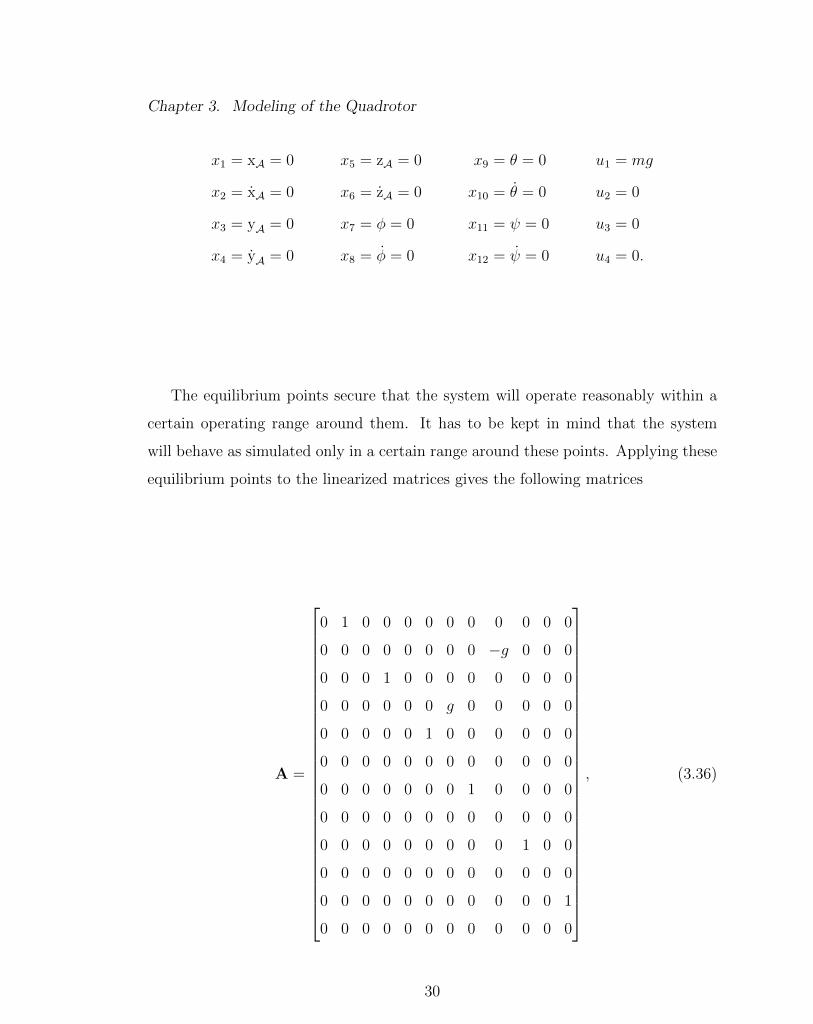
Chapter 1. Introduction
A common way to control the quadrotors is to have a ground control station, but
this has the disadvantage that it lacks flexibility. The GS has to be communicating
with the unmanned aerial vehicle (UAV) at all times, which requires that it be within
communication range.. This makes the process of going from an indoor motion
capture environment to a more realistic outdoor environment difficult. Additionally
a communication delay is introduced, since the position feedback has to first go to
the GS and then the GS sends control inputs to the quadrotor.
The purpose of this thesis is to develop a flexible high performance on-board
control architecture for aerial vehicles in the Multi-Agent, Robotics, Hybrid, and
Embedded Systems (MARHES) Laboratoy at the Univeristy of New Mexico. The
goal is to have an on-board microprocessor interfaced with different vehicles in order
to perform various applications, which then can be implemented reliably with mini-
mum effort. Previosly the quadrotors in the MARHES testbed have been controlled
off-board using LabView [11] or on-board using an Intel Edison microprocessor [12].
Eliminating the GS in the architecture will decrease the position feedback delay to
make the UAVs more robust and high performance. A picture of the marhes testbed
can be seen in Figure 1.1. The architecture makes it possible to replace the Vicon
position feedback with camera position information which allows the quadrotor to
fly outside the restricted area.
ROS has been evolving over the last several years as the robotic communication
system of choice on the Ubuntu operating system. It has capabilities which have not
been seen before. It is developed by specialists in different robotic exercises and can
be used without charge by the community. It lifted robotic implementations to a
whole new level. There are ROS packages for almost every robot or sensor, which can
be easily manipulated and used in its node/topic environment, to implement basic to
extraordinary applications. Due to its capabilities it is part of almost every robotic
research laboratory and many industrial application [13–15]. Additionally it offers
2

Chapter 1. Introduction
the open-source physical simulator Gazebo, which offers detailed models of almost
every robot. The controllers can be implemented and tested in Gazebo and copied
almost one to one to the real system, which makes the whole process faster and safer.
The smaller, lighter and faster microprocessors, like Odroid, Rasperry Pi or Nvidia
Jetson allow for the on-board use of Ubuntu and ROS resources. This makes the
robot more interesting due to its advanced capabilities of on-board processing and
elimination of a GS, if desired.
Figure 1.1: Drawing of the MARHES testbed with quadrotors in the Vicon motioncapture area. The UAV in the front is able to go out of the Vicon area by gettingposition information from a camera.
1.2 Problem Statement
The main goal of this thesis is to implement a real-time high performance control
architecture for UAV’s. To achieve this, a ROS based high level architecture has to
3

Chapter 1. Introduction
be implemented for an on-board microprocessor. This allows for independence of the
vehicle type. It is possible to use an AscTec AutoPilot or Pixracer flight controller
with any kind of configuration of the body, as long as the attitude controller is
accordingly tuned and the high level controllers are similar. The interface setup
allows for extraction and use of real-time data from the quadrotor or motion capture
system at any point. The quadrotor must be able to be controlled with position,
velocity and/or acceleration commands.
To achieve this goal, certain subgoals have to be met along the process. A model
of a rigid body quadrotor is derived. Linear position control has been developed and
implemented. The control has to demonstrate that it is able to takeoff, land, hover,
follow waypoints, follow velocities and track trajectories. The ROS framework has
to be able to interface with MATLAB and execute trajectories that were developed
in Matlab. It also has to fly in a stable manner, even with off-centered balance.
It will be evaluated with different applications that were developed to demonstrate
the flexibility of the vehicle. A framework for a flying inverted pendulum will be
developed and shown in Gazebo, to explore the possibility of implementing it in the
MARHES laboratory.
1.3 Related Work
In the past few years, the quadrotor has become more popular and has been well
studied in papers that show many types of stabilization techniques, controllers and
models. The nonlinear model, which assumes a rigid body configuration has been
derived using Newton-Euler formalism or Lagrangian [6]. This work describes in
detail the dynamic model of a x-configuration quadrotor with all forces, moments,
inertias, etc., that act on it. The difference between a x-configuration and plus-
configuration is in the control matrix [7]. Usually the low level controller is stabilizing
4

Chapter 1. Introduction
the attitude. It can be seen that there is a tendency towards PD, PID controllers or
nonlinear controllers. All three variations have proven to be good solutions and can
be used in aggressive maneuvers [16, 17].
Different applications of quadrotors have been exploited. As an example, loads
have been modeled hanging from the aerial vehicle to reduce swinging [18]. Agile
adaptive control is implemented to correct the switch in the center of mass. These
systems can be used in aerial transportation. It has been simulated and tested in the
MARHES Testbed. Additionally quadrotors could be used for carrying information
between ground agents. Many micro robots could be implemented in order to take
pictures or collect information about the environment. The quadrotors could be
used in this environment to collect the data from the ground-robot via an optical
link and relay it to a home station [19]. A lot of research has been devoted to
reachability analysis, where the quadrotor or a group of quadrotors could catch a
potential threat [20, 21].
Additionally, a quadrotor could be used as an aerial Segway or flying taxi. A
model of an inverted pendulum on a quadrotor would be needed for this type of
application, which has been done for a linear and rotational inverted pendulum.
Swing-up and balancing controllers have been developed for both cases, where it is
usual to swing-up the pendulum with an energy controller and balance it with an
LQR controller [22–25]. Researchers at ETH Zurich have already implemented flying
inverted pendulums, which are balanced in the center of the quadrotor. The UAV’s
are able to balance the pendulum as well as throw and catch it from one quadrotor
to another, respectively [26, 27]. For the throwing maneuver an optimal path of the
quadrotor to the pendulum launch is derived, as well as an optimal catching instant.
The simulation and experiments have been published and demonstrated in the Flying
Machine Arena.
All the work that is presented in this sections show the ability and flexibility of
5

Chapter 1. Introduction
quadrotors. A desire to have a general architecture which can be used for various
applications to simplify the implementation process as well as the performance can
be seen.
1.4 Organization of this Thesis
In the following chapter the different hardware and software used throughout the the-
sis is presented. It includes detailed descriptions of vehicles, their sensors, the motion
capture system, on-board microprocessor and the Robotic Operating System. Their
characteristics and advantages/disadvantages will be shown. In Chapter 3 the model
of the quadrotor will be derived using Newton-Euler formalism. The differences be-
tween a x-configuration and plus-configuration will be explained. Additionally, it
will describe the ROS architecture and implementation of the on-board microproces-
sor. Chapter 4 shows different applications that demonstrate the flexibility of this
architecture. Chapter 5 will show the development of a control strategy that will be
able to swing up and balance a flying inverted pendulum in a linear and rotational
manner. It includes the model, controllers for swing-up and balancing, stability
analysis using Lyapunov, Gazebo implementation and preliminary implementation
results. Chapter 6 will be a conclusion and discussion of future possibilities of the
framework.
6

Chapter 2
System Overview
2.1 Hardware
2.1.1 MARHES Testbed
The heterogeneous MAHRES Testbed at the University of New Mexico consists
of a variety of different ground and aerial vehicles. The ground rovers are three
TurtleBot2 [28], five Pioneer 3-AT [29] and ten TXT-1 body based monster trucks
[30]. Additionally there are currently two different bio-inspired crawling robots,
the OctoRoACH [31] and five miniROaCHes [32], which are a modification of the
Kamigami Dash robot. The flying robots used in the MARHES testbed are three
AscTec Hummingbirds [33], seven Pixracer based quadrotors with QAV250 frame and
a custom made Pixracer based multirotor. Furthermore, two humanoid Baxter [34]
robots are part of the laboratory. For exact position feedback a Vicon MX [35]
motion capture system is used. A safety net is installed in the testbed area for
security reasons. The MARHES laboratory, with a majority of the robots, can be
seen in Figure 2.1. Odroid XU-4 [36] or Nvidia Jetson TK1 [37] are used as on-board
7

Chapter 2. System Overview
microprocessors for the aerial vehicles, whereas the miniRoACHes are developed with
a Raspberry Pi Zero W [38] as the on-board computer.
Figure 2.1: Heterogenous MARHES Testbed with a variety of humanoid, ground andaerial robots in the Vicon motion capture area.
2.1.2 AscTec Hummingbird
The AscTec Hummingbird quadrotor is typical vehicle used in research due to its
advanced capabilities, open-source software and extensive resources that are provided
by research groups on-line. The UAV can be seen in Figure 2.2. Designed for research,
it has the capability of high performance flight maneuvers and, due to its design, is
easy to repair [33]. It is designed to fly in a plus configuration, which means that the
front extends along one of the arms, which can be seen by the orange tape attached
in the picture.
It comes with the Ascending technologies AutoPilot, which is able to run Low-
Level(LL) attitude control loops including the process of collected sensor data with
8

Chapter 2. System Overview
data fusion at 1000Hz. It is possible to run custom High-Level controllers on the
provided High-Level(HL) processor, however for this thesis the HL processor is only
used to interface the Odroid-XU4 microprocessor and pass the desired inputs to the
LL controller. The board can be interfaced with GPS provided by AscTec for outdoor
implementations. For safety, AscTec is providing several emergency modes that
can be essential to rescue the vehicle before a disaster happens. The HL processor
provides a serial interface which is used to get information from radio receivers,
XBee receivers or other serial interfaces. For this thesis it will communicate with
the Odroid to implement position, velocity or acceleration control at a bau drate of
921600.
Figure 2.2: AscTec Hummingbird quadrotor with Odroid XU4 microprocessor ontop of it and Vicon markers attached.
The Hummingbird uses specific Electronic Speed Controllers(ESC) and motors
developed for it. This guarantees flawless interfacing with the AutoPilot. The motors
are designed for improving efficiency as well as maneuverability in combination with
the ESC’s. The 1000kV motors paired with the 12 inch propellers only need 100W
9

Chapter 2. System Overview
per motor. This implementation makes it possible to reach flight times of up to 30
minutes if there is no payload attached to the quadrotor. Each motor is able to
approximately generate 5N of maximum thrust. The maximum takeoff weight for
the quadcopter is given to be 710g, and having a weight of 510g it allows for 200g
of extra payload that can be attached safely. The batteries used for the UAV are
3s Lipo batteries, which are light but also less powerful than higher cell batteries.
The 3 Cell batteries provide a voltage of 12.6V when they are fully charged. The
batteries used for this thesis have a rating of 1800mAh.
Additionally, the body structure is very lightweight, which also helps to increase
efficiency as well as a agility. The core of the hummingbird is made out of three levels
of carbon fiber plates for stiffness and weight reduction. These levels are connected
by four magnesium structures which add stability to the frame. The arms are made
out of two carbon fiber plates which are connected through a layer of balsa wood.
This makes them structurally stiff, but the main advantage is that the wood layer
makes them extremely light weight. The diameter from motor to motor is 36.5mm
which makes it a Mini Rotorcraft Unmanned Aerial or Aircraft System(RUAS) [39].
2.1.3 QAV250
The QAV250 based quadrotor has been developed as part of a project with Sandia
Laboratories. It was developed to have a small UAV with extensive maneuverability
and payload capacities. The vehicle has been built from scratch, which allowed for
a variety of components to choose from to produce the best output. It can be seen
in Figure 2.3. It flies in a x-configuration.
For the flight controller, the PixRacer is used due to its compatibility with ROS
and its extensive resources [40]. It is able to communicate with the on-board com-
puter over USB. Its attitude controller is running at 400Hz, whereas it is getting
10

Chapter 2. System Overview
Accelerometer, Gyroscopic and Magnetometer updates at 4000Hz. One of the main
advantages is that it is compatible with OneShot ESC protocol. This increases the
flight performance, because the Flight Controller(FC) and ESC synchronize their
loop-time, which eliminates the error of reused PWM signals without OneShot. Fur-
thermore, the signal sent from FC to ESC is shorter, 125us-250us compared to 1ms-
2ms. With OneShot protocol comes a feature called Active Braking, this will actively
brake the motor when the speed is supposed to be decreased by applying reversed
voltage, instead of applying less volts and waiting until the desired propeller speed is
reached. These factors lead to a increase in quadrotor response, which adds stability,
agility and maneuverability. Additionally, it has several telemetry, GPS and radio re-
ceivers that work with almost all equipment that is used in the Radio Controlled(RC)
vehicle sector. Its small footprint (32mmx32mm) allows it to be implemented in small
body frames.
Figure 2.3: QAV250 frame based quadrotor with Odroid XU4 microprocessor on topof it and Vicon markers attached. The Odroid is secured by a custom design and 3Dprinted part.
The ESC used to convert the FC signals to motor outputs are Lumenier F390
11

Chapter 2. System Overview
30A, which come with OneShot and Active Breaking capabilities, when configured
on the FC side. They withstand 30A continuous and 40A burst for 10 seconds. Its
powerful F390 chip allows for fast response. Cobra 2205 size motors with 2500kV
were choosen due to their quality and extreme thrust generation. Their advanced
bearings allow almost frictionless rotation. In combination with 5 inch propellers
and 16V they are able to produce 1.5kg thrust per motor. The combined maximum
thrust of 6kg is an advantage, since the complete quadrotor weights approximately
820g with battery it is able to handle securely an additionally 3kg payload.
The Lumenier QAV250 frame is a two level x-type frame. It has a motor to motor
diameter of 250mm. The 3k carbon fiber structure adds stiffness to the quadrotor
in addition to being light-weight. The design allows the quadcopter to withstand
even strong impacts. Considering the size, weight and payload capability it can be
counted as a small-scale RUAS [39].
2.1.4 Vicon System
The MARHES laboratoy Vicon system is used for position and orientation feedback
for the aerial vehicles. The high precision, fast update rate, simple setup, friendly user
interface and extensive resources make it a perfect research resource to implement,
test and tune control algorithms. It consist of 8 cameras and an MX Giganet which
collects all of the camera feedback and interfaces a computer running Vicon Tracker
software on Windows 7 Operating System(OS) [35]. It delivers high-precision vehicle
data with an error down to 0.5mm in the position and 0.5deg to the rotation at
an update rate of up to 225Hz. The Bonita cameras operate at 240 frames per
second(fps). The cameras have red LED’s which are reflected by the markers, as seen
in Figure 2.2 and 2.3, to get feedback of a predefined object. The setup schematic
of the Vicon area can be seen in Figure 2.4. In the picture the Ethernet connections
12

Chapter 2. System Overview
are shown by the solid lines and the Wifi connection can be seen by the dotted line.
Figure 2.4: Schematic of the Vicon system and its setup in the laboratory.
The Tracker software is the interface between the computer and the MX Giganet.
First the cameras have to be calibrated using the Vicon Wand seen in Figure 2.5a.
Next the user is able to set the origin with the same wand, where the long end marks
the x-axis. The coordinate system follows a East-North-Up system, which means
that z is up, y to the left and x is to the front. The markers have to be attached
on the robots next in an asymmetric order, so that Vicon is able to see differences
between the agents. It is then possible to create a model in the Tracker software,
which can be published to the network. Every robot that is connected to the same
router via Ethernet or wireless is able to run ViconStream code, which is provided
for Windows, Ubuntu and MAC OS by Vicon. A picture of the virtual created room
in Tracker can be seen in Figure 2.5b and a close range view of the created Vicon
13

Chapter 2. System Overview
(a) Vicon Wand to setupthe Vicon area.
(b) Vicon area showing thecreated area, each of thecameras and 2 objects.
(c) Close look at an objectin the tracker software.
Figure 2.5: Vicon equipment for setup and view of Tracker software.
model in the real-time position and orientation tracking system is seen in Figure
2.5c. It shows a close range view of the object created with the markers and the
origin for this object. The position and orientation of this origin is the published by
Vicon, and it is possible to manipulate the origin of an object if needed.
2.1.5 Odroid XU4
The Odroid XU-4, which can be seen in Figure 2.6, has been chosen due to its
enhanced capabilities and small size [36]. Some relevant characteristics given by the
developer are
• CortexTM-A15 2Ghz and CortexTM-A7 Octa core CPUs
• 2Gbyte LPDDR3 RAM PoP stacked
• eMMC5.0 HS400 Flash Storage
• 2 x USB 3.0 Host, 1 x USB 2.0 Host
• Size : 83 x 58 x 20 mm
14

Chapter 2. System Overview
Figure 2.6: Odroid XU4 microprocessor from Hardkernel.
• Linux Kernel 4.9 LTS
The 64 bit memory bandwidth processor in combination with the 2Gb RAM
gives enough calculation power to run advanced programs, especially for an on-board
computer. Similar microprocessors are significantly less powerful, as an example the
Odroid is approximately 7 times faster than the latest Raspberry PI 3. For this thesis
32gb eMMC cards are used, which are approximately 4 times faster than high quality
MicroSD cards. The storage makes it possible to use Lubuntu 14.04 as the operating
system with a desktop version of ROS. The serial connector gives the ability to
connect the Odroid XU4 with the AscTec AutoPilot board and the USB 3.0 port is
used to connect to the Pixracer FC. In both cases, one of the USB 3.0 port is used for
the WiFi adapter to get fast high precision Vicon position and orientation updates
from the Router. The small footprint of the microprocessor makes it possible to fit
it on small quadrotor bodies. Parts to mount the Odroid on the different multirotor
bodies have been designed and printed. The light weight of 38 grams does not add
a lot of payload to the UAV’s, which makes it a reasonable choice.
15

Chapter 2. System Overview
2.2 Software
2.2.1 ROS
The Robotic Operating System has become the standard for robotic research. It is
an open source free of charge meta-operating system [41]. It combines the following
services
• operating system
• hardware abstraction
• low-level device control
• message-passing between processes
• package management
The robot framework additionally provides libraries to obtain, build, write and run
code. The communication infrastructure is the main advantage of ROS. It makes
it as simple as possible to use different robots or sensors and interface them with
each other. It is a node and topic system. Nodes are essentially Python Code or
C++ programs downloaded or specifically built by the users which can subscribe or
publish to different topics. As soon as a topic is published each node has the ability
to subscribe to it. This concept can be seen in Figure 2.7. The ROS Message Types
are predefined or custom messages, which define the format of how the information is
published. There are basic messages which are efficient and well arranged, however
advanced users can also create their own message types if needed.
ROS was designed to interface with Ubuntu, which is used as a typical research
operating system, due to its capabilities and the fact that it is free of charge. Over the
16

Chapter 2. System Overview
Figure 2.7: Publish/Subscribe concept of topics by nodes in the Robotic OperatingSystem [1]
years there have been several distribution versions of ROS. A table of ROS version,
their Ubuntu compatibility and end of support date can be seen in Table 2.1. The
ROS version used throughout the thesis is ROS Indigo Igloo. It has the advantage
that it is mainly made for Ubuntu 14.04, which is a Long Term Support version of
Ubuntu that added security to the project. Ubuntu 14.04 also has a light version,
called Lubuntu which interface with the Odroid-XU4. The user has the ability to
install different versions of ROS, which are the Full Desktop, Desktop, Bare-Bones
and Individual package version. The difference between them are essentially the
amount of packages that come predefined with them, which correlates to the storage
amount needed for the version. Whereas on a ground station one would install
the Full-Desktop version, for the on-board computer, the desktop version has been
chosen. It ensures that not to much of the 32gb memory storage of the Odroid
XU4 eMMC card is used and is still sufficient. Additionally, specific packages are
needed later on they can be installed manually, so there is no real drawback of using
a lighter version other than the compiling time for ROS packages may take longer,
due to initially missing packages.
For the communication between the Odroid XU4 and AscTec AutoPilot the
asctec mav framework ROS package is been used. This package is supported up
17

Chapter 2. System Overview
ROS Version Ubuntu Version End of Support
Lunar Loggerhead 17.04(Zesty),16.10(Yakkety)& 16.04(Xenial) May 2019
Kinetic Kame 16.04(Xenial) & 15.10(Wily) April 2021
Jade Turtle 15.04(Wily), 14.10(Utopic) & 14.04(Trusty) May 2017
Indigo Igloo 14.04(Trusty) & 13.10(Saucy) April 2019
Hydro Medusa 13.04(Raring), 12.10(Quantal) & 12.04(Precise) May 2015
Groovy Galapagos 12.10(Quantal), 12.04(Precise) & 11.10(Oneiric) July 2014
Table 2.1: ROS Distributions since December 31, 2012. Additionally, informationabout the compatibility with Ubuntu versions and end of date for their support.
to ROS Indigo. It provides communication at baud rates of 921600. Additionally,
IMU data fusion at 1kHz has been implemented in the package and is able to be
used for the attitude control. These state estimations are provided in custom ROS
messages which can be used to implement controllers on the platform. The frame-
work allows to send positions, velocities or accelerations to the quadrotor. Positions
and velocities are in the world frame which is provided by the Vicon system. For the
acceleration, the user sends a normalized thrust value (0 to 1), roll and pitch in body
frame in rad and the heading in rads
. It connects via serial communication. Since the
Odroid has a 1.8V logic and the AutoPilot board has a 3.3V logic, a simple voltage
level converter board is used to make communication possible. For The PixRacer
FC, the mavros package is used. It is developed for px4 based flight controllers, like
PixHawk, PixHawk Mini and PixRacer. The advantages of this package are the ex-
tensive resources and number of people involved in the project. It is possible to send
motion capture or vision position data to the ROS package and fuse it with the IMU
data with the desired trust in the on-board and off-board data. The quadrotor can
be controlled in various ways by sending linear and rotational positions, velocities
and/or accelerations to the PixRacer. An Extended Kalman Filter (EKF) provides
state estimation. The motion capture system is using the Vicon SDK in combi-
nation with a lightweight communications and marshaling package to optimize the
high-bandwidth communication.
18
Chapter 2. System Overview
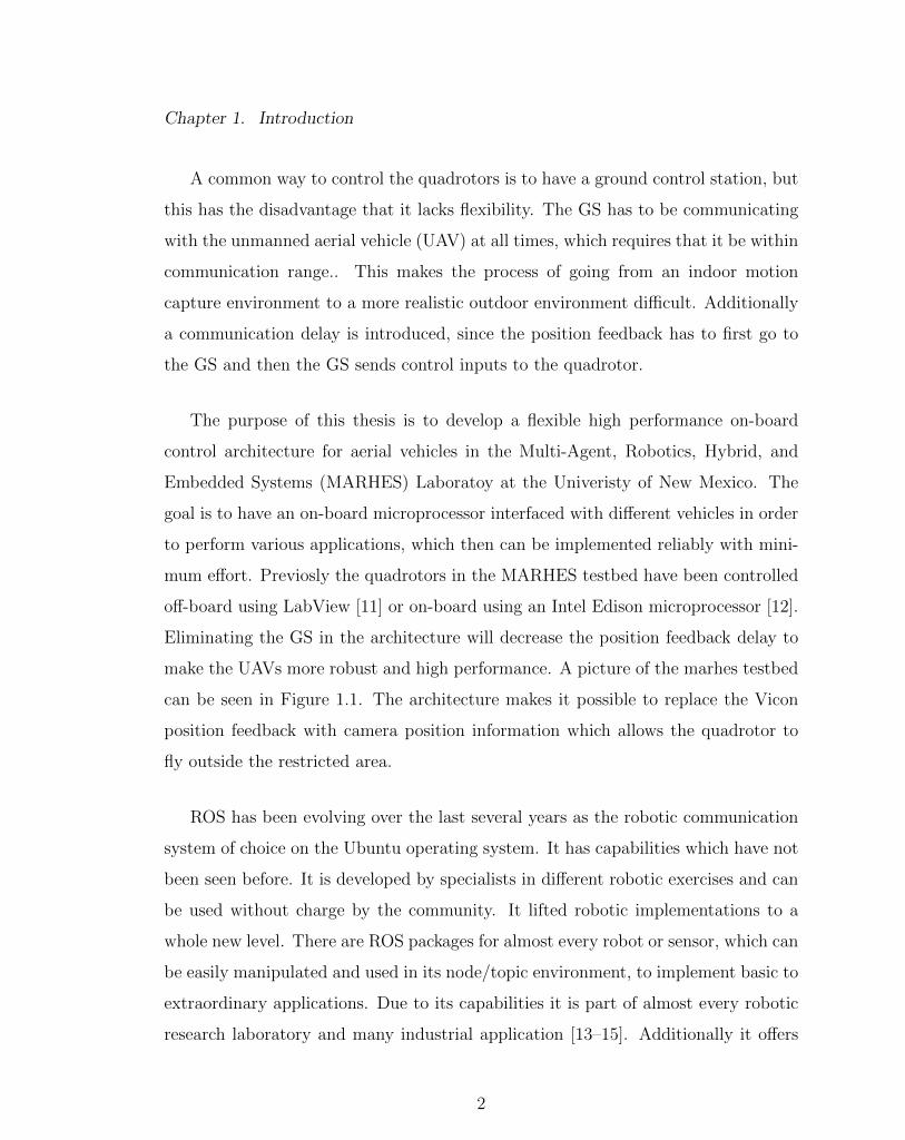
Additionally ROS provides a physical simulator which is called Gazebo [42]. Fea-
tures of Gazebo are
• Dynamics simulation - high performance physics engines
• Advanced 3D graphics - realistic rendering of environment
• Sensors and noise - model sensors with noise
• Plugins - ability to develop custom plugins for robot, sensor and environmental
control
• Robot models - many existing robots have already been modeled and are avail-
able
• TCP/IP transport - ability to run simulation from remote servers
Since Gazebo is embedded in ROS, it uses the same structure. This makes it
a useful tool, because the controllers can be created, implemented and tested in
a close to real world scenario and taken to the real robot in similar fashion. These
advantages lead to the use of the simulator for a specific application presented in this
thesis. The simulation will consider an inverted pendulum on a quadrotor and has
been completely tested in Gazebo. The rotors simulator package has been used to
get an exact replica of the AscTec Hummingbird with all its characteristics [43]. This
eliminated the need of designing the quadrotor from zero in Gazebo. A pendulum
has been modeled and attached to the quadrotor with all characteristics and inertias.
The cascade control strategy has been implemented and is explained later on in the
thesis.
Additionally a new ROS version is currently under development. Even though
new distributions of ROS are continuously developed, there were some disadvantages
that are so deep in the ROS core that a new version called ROS 2 is being developed.
19

Chapter 2. System Overview
This new version is focusing on improving support for multiple Data Distribution
Service(DDS) middleware implementations. It is being tested for more Operating
Systems, including Windows 10. It also tries to implement more programming lan-
guages. All these changes are an effort to improve the system and further adapt
to the robotics community, which has changed since ROS 1 was first introduced in
2007.
20

Chapter 3
Modeling of the Quadrotor
For the quadrotor model certain assumptions have to be made. The first assumption
is that the quadrotor is symmetrical and has a rigid body structure with 6 Degrees
of Freedom (DOF) [6, 16, 44, 45]. 3 DOF for translation and 3 for orientation. Ad-
ditionally, the propellers are also assumed to be a rigid body. The thrust and drag
created by the propellers are proportional to the square of the rotational propeller
speed. The center of mass (COM) of the quadrotor lies at the center of its body
frame.
3.1 Kinematics Model
The schematics of the model can be seen in Figure 3.1. The world frame A has the
reference axes xA, yA and zA. It can be noticed that zA is going out of the world or
up. The Euler angles which define the rotation around the axes are defined as follows,
φ is the angle around the x-axis, θ is the angle around the y-axis and ψ is the angle
around the z-axis. The body frame B of the the quadrotor is attached to its COM
and has the reference axes xB, yB and zB. The axes xB is pointing toward propeller
21

Chapter 3. Modeling of the Quadrotor
one and represents the front of the quadrotor, yB is pointing toward propeller two
and zB i pointing upwards. The distance between these two coordinate frames is r,
where r can be expressed as r = [x y z]T .
Figure 3.1: Schematic diagram of the quadrotor aerial vehicle. The world frame Ashown in black and the body frame B shown in green with their related axes. Thedistance from the origin of the world frame to the origin of the body frame is shownby r in red. The system characteristics are symbolized in light blue.
The multirotor inputs for the four motors are represented as T1, T2, T3 and T4.
T1 and T3 are rotating counter-clockwise, whereas T2 and T4 are rotating clockwise.
The distance between the center of mass of the quadrotor and the motors is shown
by Lq.
The rotational matrix ARB defines the orientation of the body frame to the world
frame, which is needed due to the fact that some states of the dynamic model are
22

Chapter 3. Modeling of the Quadrotor
measured in the world frame (i.e. gravitation and quadrotor position), and some
are measured in body frame (i.e. thrust created by propellers) [44]. The rotation
sequence used for this thesis will be Z-Y-X or 3-2-1. The quadrotor orientation is
described by roll (φ), pitch(θ) and yaw(ψ), so that the rotational matrix ARB(ψ, θ, φ)
looks as follows
ARB =
cθcψ sθsφcψ − cφsψ cψsθcφ+ sφsψ
cθsψ sθsφsψ + cφcψ sψsθcφ− sφcψ
−sθ sφcθ cφcθ
. (3.1)
It can be noted that s is the sine function and c is the cosine function. Additionally
it can be said that ARB is orthogonal.
3.2 Dynamic Model of a Quadrotor
The position of the quadrotor COM is defined in the inertial frame by ξ and the
attitude is expressed by η, so that the vector q accommodates the linear and angular
position in the inertial frame
ξ =
xA
yA
zA
,η =
φ
θ
ψ
,q =
ξη
. (3.2)
The body dynamics of the quadrotor are represented by vA, which represents the
linear velocity in inertial frame and ν, which represents the angular velocity in body
frame.
vA =
xA
yA
zA
,ν =
p
q
r
, (3.3)
23

Chapter 3. Modeling of the Quadrotor
where p, q and r represent the angular velocities in the fixed body frame. The
inertia matrix for the quadrotor is defined as follows
I =
Ixx 0 0
0 Iyy 0
0 0 Izz
. (3.4)
The inputs to the system are the four forces created by the motors [46]. The first
input is the collective thrust represent by Tf .
Tf =4∑i=1
Ti (3.5)
The force created by a single rotor can be described as follows.
Ti =1
2ρACtr
2bω
2i = ktω
2i (3.6)
where ρ represents the air density, Ct is the aerodynamic coefficient, A is the blade
area, rb is the blade radius, kt represents the force constant and ω is the rotational
speed of the blade. With the help of equation (3.6) it is possible to rewrite equation
(3.5) to
Tf = kt
4∑i=1
ω2i (3.7)
The second and third input into the system represent the torques around the x
and y body axis created by the difference of motor speeds. The moment, which is
force multiplied with the distance, around the body axis xB and yB can be described
as follows
24

Chapter 3. Modeling of the Quadrotor
τxB = T2Lq − T4Lq
= ktω22Lq − ktω2
4Lq
= ktLq(ω22 − ω2
4)
(3.8)
τyB = T3Lq − T1Lq
= ktω23Lq − ktω2
1Lq
= ktLq(ω23 − ω2
1).
(3.9)
The fourth input describes the moment around the z body frame axis. It is is
calculated by addition/subtraction of the individual moments created by each rotor.
The moments created by each motor can be described as follows
Mi =1
2ρACdr
2bω
2i = kmω
2i . (3.10)
The moment created by the i-th motor is described by Mi, Cd represents the
moment coefficient of the blade and km describes the moment constant. This equation
helps to represent the moment around zB which looks like
τzB = M2 +M4 −M1 −M3
= kmω22 + kmω
24 − kmω2
1 − kmω23
= km(ω22 + ω2
4 − ω21 − ω2
3).
(3.11)
It is known that u4 is the weakest input, due to the fact that the moment constant
km is usually smaller than the force constant kt. Combining equation (3.5), (3.8),
(3.9) and (3.11) one can develop a matrix, which includes the forces and moments
acting on the quadrotor by its inputs, which looks as follows
25

Chapter 3. Modeling of the Quadrotor
MB =
Tf
τxB
τyB
τzB
=
kt∑4
i=1 ω2i
ktLq(ω22 − ω2
4)
ktLq(ω23 − ω2
1)
km(ω22 + ω2
4 − ω21 − ω2
3)
. (3.12)
This can be redefined into the inputs for the system, where Tf is u1, τxB represent
u2, τyB defines u3 and τzB is u4. This allows to express the control matrix u as follows.
u =
u1
u2
u3
u4
=
kt kt kt kt
0 ktLq 0 −ktLq−ktLq 0 ktLq 0
−km km −km km
ω21
ω22
ω23
ω24
. (3.13)
3.2.1 Newton-Euler Approach
Using Newton-Euler formalism, the equations of motion for the translational and
rotational motion can be derived. The translational change is described in world
frame, whereas the rotational motion is described in body frame [45]. The external
forces applied to a rigid body can be described by the following equations
ξ = vA (3.14)
mqvA = f (3.15)
R = RΩ (3.16)
Iν = −ν × Iν + τ. (3.17)
Equation (3.15) describes Newton’s first law applied to the body frame, where f
described the non-conservative forces applied to the quadrotor and mq denoted the
26

Chapter 3. Modeling of the Quadrotor
quadrotor mass. The following equation describes the law to achieve the derivative to
the rotational matrix, with respect to time, where Ω represents the skew-symmetric
matrix. Equation (3.17) is used to calculate the moments around the body axis. The
non conservative forces can be separated in gravitational and translational forces, so
that f = ARBTf −mqgξz, and equation (3.15) becomes
mqvA = ARBTf −mqgξz. (3.18)
The translational forces of equation (3.18) were calculated using the statement
ARBTf , where Tf = [0 0 kt∑4
i=1 ω2i ]′ = [0 0 u1]
′ according to the input matrix
represented in Equation (3.13), so that they can be represented as follows
ARBTf =
cθcψ sθsφcψ − cφsψ cψsθcφ+ sφsψ
cθsψ sθsφsψ + cφcψ sψsθcφ− sφcψ
−sθ sφcθ cφcθ
0
0
u1
=
(cψsθcφ+ sφsψ)u1
(sψsθcφ− sφcψ)u1
(cφcθ)u1
.(3.19)
The gravitational forces only act on the altitude or z component, so that
mqgξz = mqg
0
0
1
=
0
0
mqg
.(3.20)
With equation (3.19) and (3.20) the non conservative forces for the translational
motion can be rewritten as
27

Chapter 3. Modeling of the Quadrotor
xA =(cψsθcφ+ sφsψ)u1
mq
, (3.21)
yA =(sψsθcφ− sφcψ)u1
mq
, (3.22)
zA =(cφcθ)u1mq
− g. (3.23)
For the rotational motion we can rewrite equation (3.17) toIxx 0 0
0 Iyy 0
0 0 Izz
p
q
r
= −
p
q
r
×Ixx 0 0
0 Iyy 0
0 0 Izz
p
q
r
+
τxB
τyB
τzB
=
qrIyy − rqIzz
rpIzz − prIxx
pqIxx − qpIyy
+
u2
u3
u4
=
qr(Iyy−Izz)+u2
Ixx
rp(Izz−Ixx)+u3Iyy
pq(Ixx−Iyy)+u4Izz
.
(3.24)
For small angle assumptions of the vehicle it can be assumed that there is a
relation between the rotational angles in body frame and the rotational velocity in
world frame which is φ ≈ p, θ ≈ q and ψ ≈ r [47]. This assumptions makes it
possible to rewrite equation (3.24) which becomes
φ =Iyy − IzzIxx
θψ +u2Ixx
, (3.25)
θ =Izz − IxxIyy
φψ +u3Iyy
, (3.26)
ψ =Ixx − IyyIzz
θφ+u4Izz
. (3.27)
With equation (3.21), (3.22), (3.23), (3.25), (3.26) and (3.27), which describe the
translational and rotational motion of the quadrotor, the complete model can be
built, which looks as follows
28

Chapter 3. Modeling of the Quadrotor
xA =(cψsθcφ+ sφsψ)u1
mq
, (3.28)
yA =(sψsθcφ− sφcψ)u1
mq
, (3.29)
zA =(cφcθ)u1mq
− g, (3.30)
φ =Iyy − IzzIxx
θψ +u2Ixx
, (3.31)
θ =Izz − IxxIyy
φψ +u3Iyy
, (3.32)
ψ =Ixx − IyyIzz
θφ+u4Izz
. (3.33)
The collective thrust is described by u1 and the roll, pitch and yaw moments are
represented by u2, u3 and u4, respectively. The under-actuated system has can move
in 6 degrees of freedom with 4 control inputs.
3.2.2 Linearized Model
For linear control it is important to bring the model into state space represen-
tation. First the system has to be linearized around the hovering point, which
means that u1 = mg. The states for the linearized model are chosen as follow
x = [xA xA yA yA zA zA φ φ θ θ ψ ψ]T . The linearized state space representa-
tion follows the common model, which looks as follows.
x = Ax+ Bu, (3.34)
y = Cx+ Du, (3.35)
where A is the state matrix, B the input matrix, C the output matrix and
D the feed-through matrix. The linear system has the advantage that simple and
systematic controllers can be applied which still give excellent outputs. The following
equilibrium points have been chosen
29
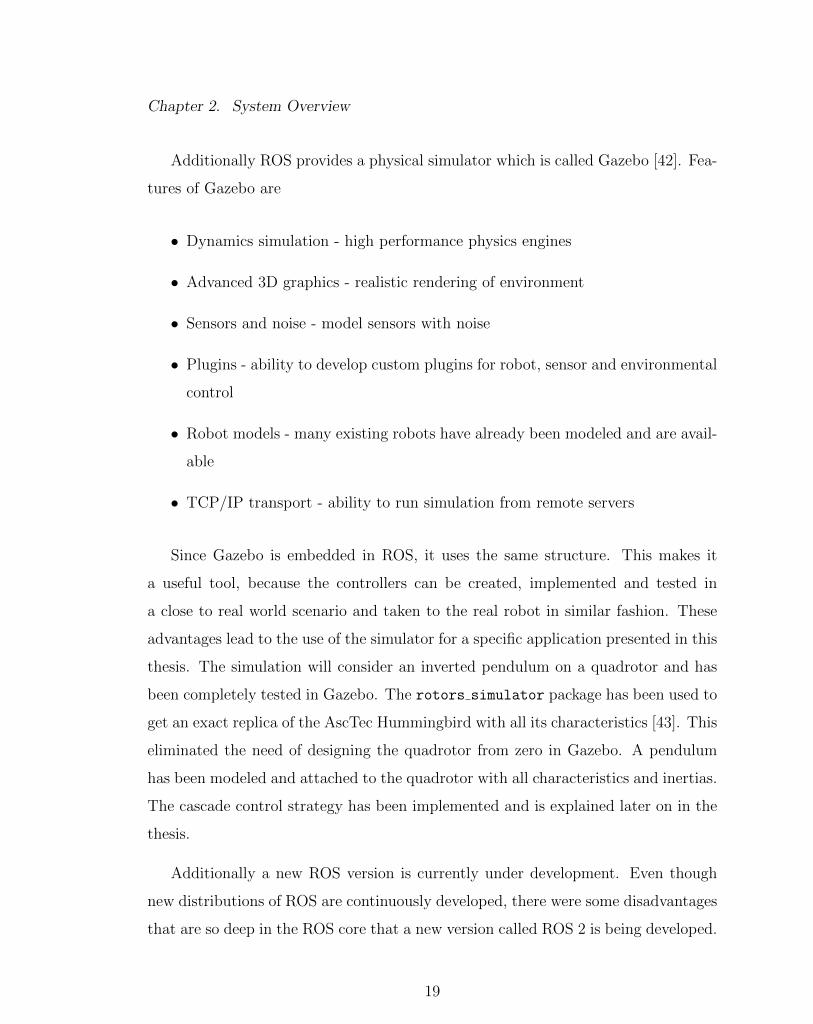
Chapter 3. Modeling of the Quadrotor
x1 = xA = 0
x2 = xA = 0
x3 = yA = 0
x4 = yA = 0
x5 = zA = 0
x6 = zA = 0
x7 = φ = 0
x8 = φ = 0
x9 = θ = 0
x10 = θ = 0
x11 = ψ = 0
x12 = ψ = 0
u1 = mg
u2 = 0
u3 = 0
u4 = 0.
The equilibrium points secure that the system will operate reasonably within a
certain operating range around them. It has to be kept in mind that the system
will behave as simulated only in a certain range around these points. Applying these
equilibrium points to the linearized matrices gives the following matrices
A =
0 1 0 0 0 0 0 0 0 0 0 0
0 0 0 0 0 0 0 0 −g 0 0 0
0 0 0 1 0 0 0 0 0 0 0 0
0 0 0 0 0 0 g 0 0 0 0 0
0 0 0 0 0 1 0 0 0 0 0 0
0 0 0 0 0 0 0 0 0 0 0 0
0 0 0 0 0 0 0 1 0 0 0 0
0 0 0 0 0 0 0 0 0 0 0 0
0 0 0 0 0 0 0 0 0 1 0 0
0 0 0 0 0 0 0 0 0 0 0 0
0 0 0 0 0 0 0 0 0 0 0 1
0 0 0 0 0 0 0 0 0 0 0 0
, (3.36)
30

Chapter 3. Modeling of the Quadrotor
B =
0 0 0 0
0 0 0 0
0 0 0 0
0 0 0 0
0 0 0 0
1mq
0 0 0
0 0 0 0
0 1Ixx
0 0
0 0 0 0
0 0 1Iyy
0
0 0 0 0
0 0 0 1Izz
, (3.37)
C =
1 0 0 0 0 0 0 0 0 0 0 0
0 0 1 0 0 0 0 0 0 0 0 0
0 0 0 0 1 0 0 0 0 0 0 0
0 0 0 0 0 0 1 0 0 0 0 0
0 0 0 0 0 0 0 0 1 0 0 0
0 0 0 0 0 0 0 0 0 0 1 0
(3.38)
and
D = 0. (3.39)
The inertias of the quadrotor are specific to the model and can easily be applied
to the matrices. The mass of the quadrotor is also model specific. The earth gravity
constant g is used which is -9.81ms2
.
31

Chapter 3. Modeling of the Quadrotor
3.3 System Architecture
In an actual system, the implementation looks a little bit different than the model.
Unless direct motor control is implemented, it is usual to use a cascade control
architecture. Normally a LL controller is controlling the attitude of the quadrotor
and a HL controller is implementing position, velocity, acceleration or similar control
that fits the specific needs. A generic control structure for the system of this thesis
can be seen in Figure 3.2.
The two different systems have their own FC, which can be interfaced with the
HL control implemented in this thesis. For the AscTec the LL controller running
the attitude and altitude control loop is the AscTec AutoPilot. For the QAV250
frame base quadrotor, the PixRacer acts as attitude controller. Both come with
their own advantages which are mainly the attitude control loop speed of 1kHz on
the AscTec and the flexibility to use electromechanical components for the PixRacer.
The attitude controller is utilized to stabilize the quadrotor. Both FC are interfaced
by the Odroid XU4, which is the HL controller. The HL side of the control is
completely implemented using ROS.
Figure 3.2: Overview of the closed loop control architecture implemented and partswhere the different controllers are running.
The implemented architecture makes it possible to generate an input signal on-
board the quadrotor, which can directly send its generated desired inputs to the
asctec mav framework or the mavros framework on the different UAV’s. These
32

Chapter 3. Modeling of the Quadrotor
desired inputs could be positions, velocities and/or accelerations. The respective
HL controllers will ensure that these points are met and send roll and pitch angles,
heading velocity and thrust values to the LL control. Additionally, it is possible to
bypass these HL control algorithms and implement your own which sends directly
desired roll and pitch angles, yaw velocity and a normalized thrust value. The
attitude controller converts these desired orientation inputs into control inputs for
the motors. Additionally, the altitude controller is converting the desired thrust in
the collective thrust input into the motors. The motor inputs are sent to the motors
and converted to thrust and momentum created by each individual motor. The
motor inputs with specific dynamics are producing the outputs of the system that
will be captured using sensors. The Vicon sensor will be used as a feedback for the
HL side of the controls. It gives feedback about the position and orientation of the
object created. This feedback can be used to estimate the velocity and accelerations
of each state. It can be said that the Vicon sensor can easily be replaced by GPS or a
camera using simultaneous localization and mapping algorithms. IMU is used for the
attitude control. It feeds the rotational velocity and linear acceleration back to the
PixRacer or AscTec AutoPilot. The inputs to the FL controllers could come from
mapping, trajectory generation, obstacle avoidance, etc. algorithms. Additionally it
is possible to add more sensors like Sonar, IR, laser, etc. for specific applications.
33

Chapter 4
Applications
The main purpose for this framework was to be as flexible as possible for different
applications. The ROS framework has to be designed to work with multiple het-
erogeneous robots and communicate with them. The two main projects that the
quadrotors are used for are the Micro Autonomous Systems and Technology(MAST)
and Aerial Suppression of Airborne Platforms (ASAP) project implemented by the
MARHES laboratory. The focus and implementation of these projects will be dis-
cussed.
4.1 MAST
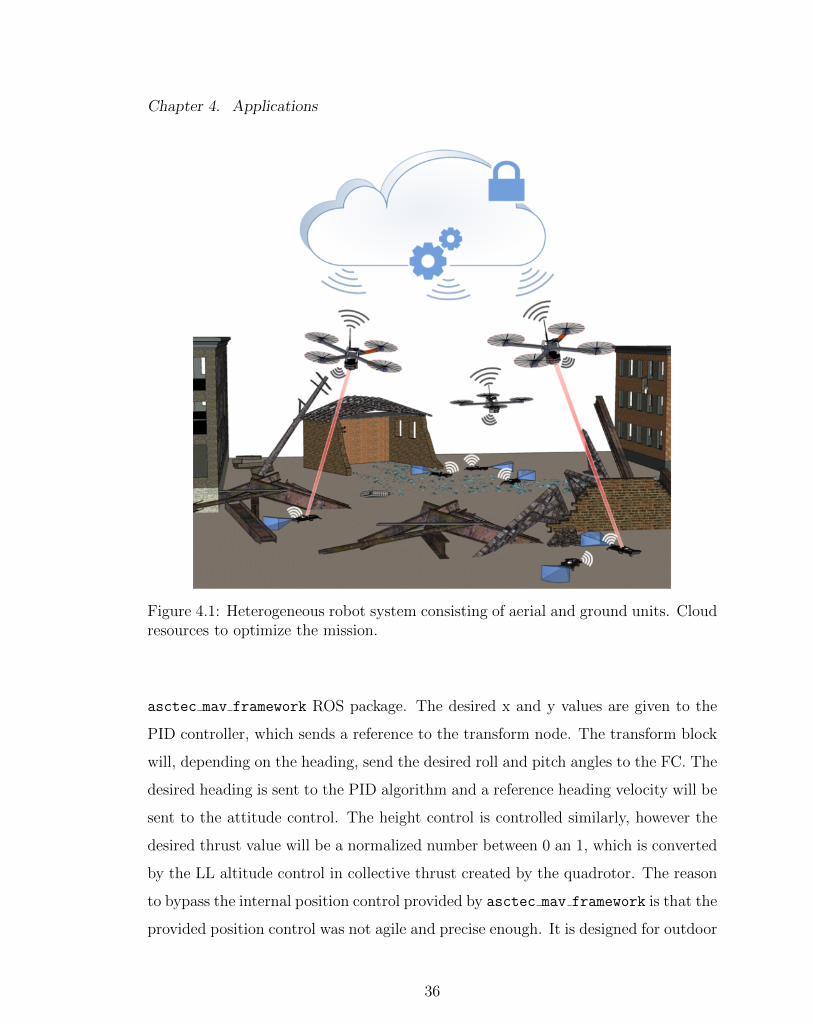
4.1.1 Introduction
For the MAST project, the MARHES lab is developing a system which is able to ef-
fectively deploy and coordinate a network of heterogeneous robots, as seen in Figure
4.1. The idea is to be able to use small and cheap universal ground robots that map
specific information of an area and send it via an optical link to aerial vehicles. The
34

Chapter 4. Applications
aerial vehicles can sufficiently get information from multiple ground robots and bring
it to a home station which would act as a cloud. Using the strength of node of the
whole system makes it possible to overcome limitations of specific robots. The cloud
is then powerful enough to use this information and extract what it needs. Such a
framework would be helpful in situations like surveillance of complex environments,
search and rescue, localization of targets, etc. The advantage of having an optical
link between the ground robots and aerial robots is that it has a robust high com-
munication rate. An optical link can only be jammed if the intruder is physically
between the transmitter and receiver, which makes it interesting for security applica-
tions. As ground robots, the Kamigami Dash robots have been modified so that they
have ROS on-board a Raspberry Pi zero. They are equipped with cameras and will
take pictures of the environment. When their internal storage is full the quadrotor
will fly above them and extract the data. The quadrotor will then fly to a ground
station, which will represent the cloud and upload the data, so that it will be able to
go back and get more information as soon as it has uploaded all data to the ground
station. For this application, the quadrotor has to be able to do waypoint navigation
and hover above an object to transmit and receive data. The quadrotor used for
this application is the AscTec Hummingbird due to its advantage of superior flight
time of up to 20 minutes. First the waypoint architecture will be discussed. Then a
velocity estimator for the controller is implemented and tested before the results of
the implemented linear control are presented.
4.1.2 Architecture
For the waypoint navigation, a position control which sends roll and pitch angles,
yaw velocity and a normalized thrust reference directly to the LL controller has
been developed. It is a PID controller and the schematic can be seen in Figure 4.2.
The Odroid XU4 is still used as microprocessor running the HL controller with the
35
Chapter 4. Applications
Figure 4.1: Heterogeneous robot system consisting of aerial and ground units. Cloudresources to optimize the mission.
asctec mav framework ROS package. The desired x and y values are given to the
PID controller, which sends a reference to the transform node. The transform block
will, depending on the heading, send the desired roll and pitch angles to the FC. The
desired heading is sent to the PID algorithm and a reference heading velocity will be
sent to the attitude control. The height control is controlled similarly, however the
desired thrust value will be a normalized number between 0 an 1, which is converted
by the LL altitude control in collective thrust created by the quadrotor. The reason
to bypass the internal position control provided by asctec mav framework is that the
provided position control was not agile and precise enough. It is designed for outdoor
36

Chapter 4. Applications
environments with GPS feedback, so the focus was on robustness and reliability.
Using Vicon as position feedback gives less noise with higher precision.
Figure 4.2: Control schematic for waypoint following of AscTec Hummingbird. Theasctec mav framework controllers are bypassed and only used to send angles andthrust references to the LL attitude controller.
The PID controllers for each state look as follows
xr = Kpxex(t) +Kix
∫ t
0
ex(τ)dτ +Kdxdex(t)
dt, (4.1)
yr = Kpyey(t) +Kix
∫ t
0
ey(τ)dτ +Kdxdey(t)
dt, (4.2)
ψd = Kpψeψ(t) +Kiψ
∫ t
0
eψ(τ)dτ +Kdψdeψ(t)
dt, (4.3)
thrustd = Kpzez(t) +Kiz
∫ t
0
ez(τ)dτ +Kdzdez(t)
dt, (4.4)
,where xr, yr, ψ and thrustd are the inputs into the system. xr and yr are a
reference that goes into the transform, and the transform calculates the desired roll
and pitch that go to the LL controller. Kp, Ki and Kd are the tunable control gains.
The error is shown by e.
37

Chapter 4. Applications
Figure 4.3: Waypoint following results for AscTec Hummingbird on-board build incontroller vs. custom linear controller.
4.1.3 Velocity Estimator
The velocity estimator has been used for the derivative part of the PID control
algorithm. Different methods have been taken into account which are the Two-Point
Derivative, Three-Point Derivative and Al-Alaoui Derivative [48]. These derivatives
38

Chapter 4. Applications
Figure 4.4: Waypoint following results for AscTec Hummingbird on-board build incontroller vs. custom linear controller.
can be calculated as follows
Two-Point : vx =x(k)− x(k − 1)
Ts, (4.5)
Three-Point : vx =x(k + 1)− x(k − 1)
2Ts, (4.6)
Al-Alaoui : vx = −1
7vx(k − 1) +
8(x(k)− x(k − 1))
7Ts, (4.7)
39

Chapter 4. Applications
where x and vx are the position and velocity, respectively. It can be noticed that the
two point estimator is a linear estimation between two points, this works very well
if there is no noise in the system. Even though the Vicon system provides reliable
feedback, a small amount of noise is amplified in the velocity. This can lead to
problems, especially with small step sizes. The three point derivative is less affected
by noise due to the fact that it is taking linear measurements of 2 time steps. The
real-time implementation problem is that it requires a future measurement. The
Al-Alaoui velocity estimation is taking the previous measurement into account. The
comparison of the estimators in the real implementation can be seen in Figure 4.5.
Figure 4.5: Comparison of the velocity estimator algorithms explained.
It can be seen that the three-point estimator is ahead by one time step. This
is due to the fact that the estimation takes future measurements into account. The
two-point and Al-Alaoui estimator perform similarly, whereas it can be noted that
the spikes of the Al-Alaoui algorithm has higher peaks. Taking this into account,
it has been decided that the Two-Point estimation is the best one for the real-time
implementation and will be used for the PID position control.
40
Chapter 4. Applications
4.1.4 Demo
As explained before, there will be one or more quadrotors in the demo. The UAV’s
are supposed to transport information from ground robots to a ground station. The
quadrotor performance has been tested and the ROS framework has been imple-
mented and tested. To be able to go from agent to agent, the UAV gets the position
feedback of the ground robots. The results of the test can be seen in Figure 4.6.
It shows the quadcopter switching between ground agents. In the blue region it is
Figure 4.6: Quadcopter approaching different ground vehicles. In the blue region ittries to hover over the base station, in the red region it follows a stationary KamigamiDash robot, and in the green region it tries to follow a moving Kamigami Dash robot.
41

Chapter 4. Applications
trying to hover over the ground station, to get information from the Kamigami Dash
robots. Then it moves towards the first stationary Kamigami, which is shown by
the red region. When it received all the information it needed it goes to the next
Kamigami, which is shown by the green region. This Kamigami is moving and the
quadrotor is following it. When it receives all of the information it needs from the
ground robot it flies back to hover over the ground station, where it can upload all
the data it has collected. It can be seen that the quadrotor is able to switch between
ground units, and is able to hold position reliably if the ground robot is not moving.
If the ground robot is moving, it hovers above it with some position latency, however
it is still performing well enough to be in the region of getting information. The
ROS framework on each node in the system made it simple to communicate between
robots and get information about their status.
4.2 ASAP
4.2.1 Introduction
Due to the increase of personal and commercial aerial vehicles in the last few years,
more research is being conducted on security in possible threat situations. This
includes detection, tracking, and neutralization. The research proposed here works
towards a threat capture system. First, when a threat is detected, forward stochastic
reachability analysis is used to evaluate the exact future probability distribution of
the threat from its current location. This is followed by an optimal control problem
to optimize the capture probability [21]. This novel approach has been developed
and tested in the MARHES lab. The quadrotors used for this experiment is the
QAV250 with on-board microprocessor.
42

Chapter 4. Applications
Figure 4.7: ASAP project. The idea of vehicle detection, tracking and neutralization.
4.3 System Schematic
The control architecture for this project makes use of the implemented position con-
troller included with the ROS packages. This makes the implementation simple and
saves time. Since the reachability analysis is running in Matlab and it needs Mat-
lab functions, the implementation makes use of the new developed Matlab Robotics
Toolbox. This toolbox makes it possible to receive and send ROS messages that
can be integrated in the framework. The system schematic can be seen in Figure
4.8. Matlab is calculating way-points for the pursuer and threat. The polyfit
function is computing trajectory coefficients for a third order polynomial that are
sent to the quadrotors. The quadrotors execute these trajectories on-board and are
able to switch their trajectories for a receding horizon environment in which updated
coefficients get sent continuously.
43
Chapter 4. Applications
Figure 4.8: System overview of the implementation.
4.4 Trajectory Tracking
For the implementation of the project, a trajectory generation based on 3rd order
polynomials has been implemented. This guarantees smooth path generation of way-
points. The coefficients are sent to the quadrotor. The quadrotor is able to execute
the trajectory with respect to time. The xA, yA and zA positions are calculated as
follows
xA = ax0 + ax1td + ax2td + ax3td, (4.8)
yA = ay0 + ay1td + ay2td + ay3td, (4.9)
zA = az0 + az1td + az2td + az3td, (4.10)
where ax0, a1, ax2 and ax3 are the polynomial coefficients to calculate the position
in inertial frame. For yA, x is switched with y and for zA, x is switched with z. The
time duration is represented by td. To test the performance, a figure eight has been
flown. To generate the figure eight, a different control law for the position generation
44

Chapter 4. Applications
has been used which is able to test the system with a difficult trajectory and can be
simplified by changing the gain k. It look as follows
xA = sin(ktd) (4.11)
yA = sin(0.5ktd) (4.12)
zA = 0.2sin(0.25ktd). (4.13)
The results of the test with different gains can be seen in Figure 4.9. This shows a
2D view from above. It can be seen that at a slow speed the quadrotor is following the
trajectory precisely. For k=1.5 and k =2.0 the quadcopter is overshooting, however
it is still able to follow the trajectory. More detailed results of the tests can be seen
in Appendix A. This figure shows each position with respect to time. There it can
be seen that some delay exists in the trajectory following. The position z of the
quadrotor is a little jittery, however it is still able to follow the trajectory. These
tests give promising results and show that the quadrotor is able to follow generated
positions.
4.5 Experimental Results
The framework has been implemented in the MARHES laboratory. It is an open-
loop experiment. The reachability analysis is generating trajectories at the beginning
of the experiment. These trajectory coefficients are sent to the quadrotor which
also triggers a flag that initiates the trajectory execution loop. With the help of a
duration timer, the waypoints along the path are generated at 100Hz and send to the
on-board position controller of the UAV. Two different scenarios have been tested
and evaluated. Their positions have been saved on-board the quadrotor to generate
the results seen in Figure 4.10 and Figure 4.11. The threat can be seen in red. It
is approaching the asset. The pursuer is following the generated trajectory that was
45

Chapter 4. Applications
Figure 4.9: x vs. y graphs of figure eight trajectory tracking at different speeds
generated by the reachability analysis. It captures the threat both times before the
threat can reach the asset. When the pursuer is inside the capture region of the
threat, the quadrotors stop and the test is counted as successful. The results of the
reachability analysis look promising.
46

Chapter 4. Applications
Figure 4.10: Experimental results of Scenario 1 for the implementation of the reach-ability analysis
Figure 4.11: Experimental results of Scenarios 2 for the implementation of the reach-ability analysis
47

Chapter 5
Inverted Pendulum on a
Quadrotor
As part of this thesis a framework for an off-centered inverted pendulum on a quadro-
tor has been developed. The goal is to have a quadrotor which can swing-up and
balance the pendulum in a linear and rotational fashion. A model has been derived
using Lagrangian. It adds the pendulum state to the complete nonlinear model rep-
resentation derived in chapter 3 on page 21. The control design is presented and
discussed. The controllers for each state of the hybrid systems have been developed
and stability of the system has been tested using Lyapunov. After achieving the
LQR gain matrix for the linear and rotational inverted pendulum, as well as the
swing reduction gain matrix Kswing using Matlab, the system has been simulated.
First the balancing maneuver has been simulated in Matlab. The full gazebo imple-
mentation has been developed and shows promising results. First steps of the real
system implementation with preliminary results are shown.
48
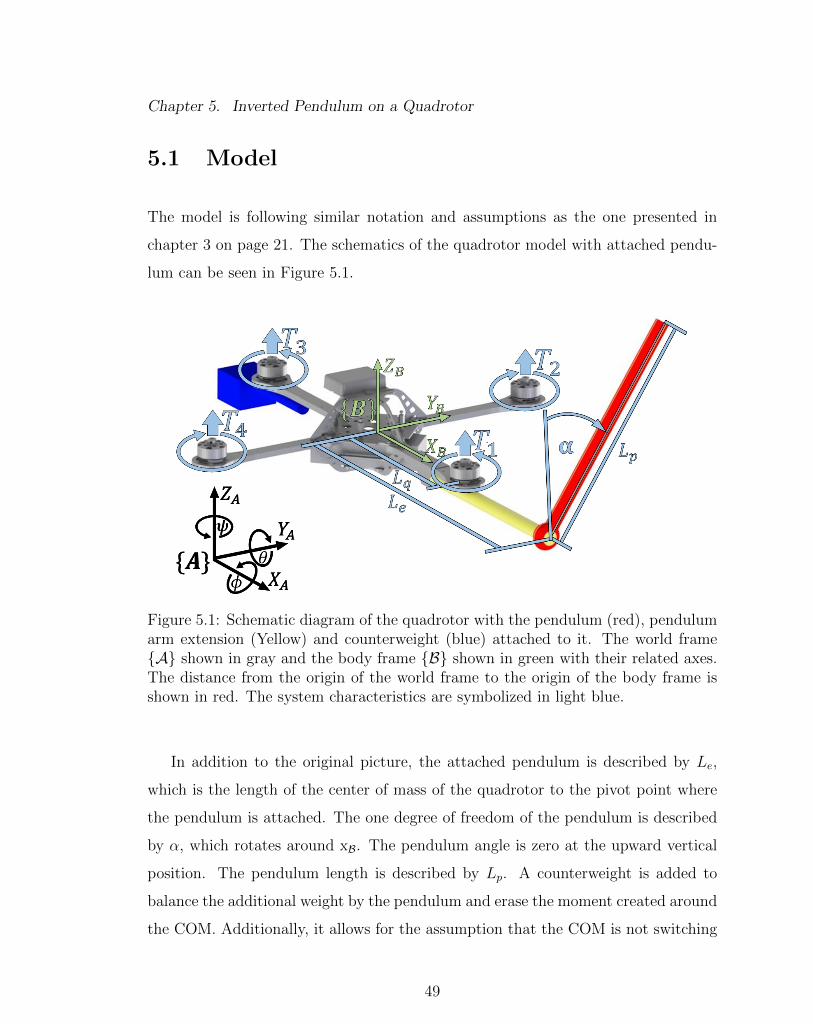
Chapter 5. Inverted Pendulum on a Quadrotor
5.1 Model
The model is following similar notation and assumptions as the one presented in
chapter 3 on page 21. The schematics of the quadrotor model with attached pendu-
lum can be seen in Figure 5.1.
Figure 5.1: Schematic diagram of the quadrotor with the pendulum (red), pendulumarm extension (Yellow) and counterweight (blue) attached to it. The world frameA shown in gray and the body frame B shown in green with their related axes.The distance from the origin of the world frame to the origin of the body frame isshown in red. The system characteristics are symbolized in light blue.
In addition to the original picture, the attached pendulum is described by Le,
which is the length of the center of mass of the quadrotor to the pivot point where
the pendulum is attached. The one degree of freedom of the pendulum is described
by α, which rotates around xB. The pendulum angle is zero at the upward vertical
position. The pendulum length is described by Lp. A counterweight is added to
balance the additional weight by the pendulum and erase the moment created around
the COM. Additionally, it allows for the assumption that the COM is not switching
49
Chapter 5. Inverted Pendulum on a Quadrotor
due to the pendulum. The mass of the pendulum attachment is given by mpand the
counterweight mass is described by mc.
The Lagrangian method is used to derive the model. The position of the pendu-
lum is given by xL =[xL yL zL
]T, respectively. Additionally the angular velocity
vector in body frame is described by ω =[ωx ωy ωz
]T.
As seen in the Figure 5.1 the pendulum is off-centered in the x-axis of the quadro-
tor body frame, so that the suspension point of the pivot can be described as (0, 0, Le)
in B [49]. The center of mass of the pendulum will be given by 12Lp. So let us
define le =[0 0 Le
]and lp =
[0 0 1
2Lp
].
Hence, q and can be defined as,
q =[xA yA zA φ θ ψ α
]. (5.1)
Furthermore, it is possible to describe the position of the COM of the pendulum
in the world frame by
xL = ξ + Rz(ψ)Ry(θ)leT + RS+
S−Rx(α)lTp . (5.2)
The pendulum angle is defined in an inverted configuration of the suspension
point reference frame, which is represented by S−. Whereas S+ reference frame
is always parallel to B. The corresponding matrix is given by
RS+
S− =
1 0 0
0 −1 0
0 0 −1
. (5.3)
The quadrotor position in world frame is defined by ξ and the pendulum positions
also in world frame are given by xL. The angular velocities of the quadrotor ω and
50

Chapter 5. Inverted Pendulum on a Quadrotor
the pendulum angle α are given in body reference frame and α is assumed to be in
the suspension point frame S−.
xL
yL
zL
=
xA
yA
zA
+
cθsψ −sψ cψsθ
sψcθ cψ sψsθ
−sθ 0 cθ
0
0
12Lp
+
1 0 0
0 −cα sα
0 −sα −cα
0
0
Le
. (5.4)
Equation (5.4) can be computed and written in full form as follows
xA
yA
zA
ωx
ωy
ωz
xL
yL
zL
=
1 0 0 0 0 0 0
0 1 0 0 0 0 0
0 0 1 0 0 0 0
0 0 0 1 0 −sθ 0
0 0 0 0 cφ sφcθ 0
0 0 0 0 −sφ cφcθ 0
1 0 0 0 Lesθcψ −Lecθsψ 0
0 1 0 0 −Lesθsψ Lecθcψ cα
0 0 1 0 −Lecα 0 12Lpsα
xA
yA
zA
φ
θ
ψ
α
(5.5)
which can be presented by
x = J(q)q. (5.6)
For the Lagrangian method the potential and kinetic energy has to be calculated.
The kinetic energy of the complete system can be expressed as follows,
T =1
2xTQMQxQ +
1
2xTLMLxL +
1
2ωT Iω +
1
2IP α
2, (5.7)
or
51

Chapter 5. Inverted Pendulum on a Quadrotor
T =1
2xTMx =
1
2qTJ(q)TMJ(q)q +
1
2IP α
2. (5.8)
The matrix M = diag([mq,mq,mq, Ixx, Iyy, Izz,mp,mp,mp]). The mass of the
quadrotor is represented by mq and the pendulum mass is represented by mp. The
pendulum inertia is shown by IP and the quadrotor inertia’s are shown by Ixx, Iyy
and Izz about x, y and z axis.
Now that the kinetic energy is calculated, the potential energy calculation is the
next step, It is given by Vp, which looks as follows
Vp = mqgzq +mqg(zQ − L sin θ − L cosα). (5.9)
Since the kinetic and potential energy expressions have been calculated, it is
possible to evaluate the Lagrangian,
L = T − Vp. (5.10)
The Euler-Lagrange equation can be used to calculated the dynamics of the off-
centered pendulum attached to the quadrotor [50],
d
dt[∂L∂q
]− ∂L∂q
= fext, (5.11)
which can be written as,
d
dt[Wq]− 1
2
∂
∂q[qTW]q +
∂V
∂q= fext. (5.12)
We obtain
Wq + (W − 1
2
∂
∂q[qTW])q +
∂V
∂q= fext. (5.13)
52

Chapter 5. Inverted Pendulum on a Quadrotor
From Equation (5.13), one can obtain the mass, Coriolis and gravitational terms
for the equation of motion of the flying inverted pendulum which looks as follows,
Mq + C(q, q)q + G(q) = fext, (5.14)
where W = JT (q)MJ(q) + diag([0, 0, 0, 0, 0, 0, 0, IP ]).
With these equations it is possible to get the complete model of the system.
Additionally, it has to be said that it is assumed that the pendulum mass is so small
that it does not affect the quadrotor. The quadrotor complete nonlinear model can
be written as
xA =(cψsθcφ+ sφsψ)u1mq +mp +mc
, (5.15)
yA =(sψsθcφ− sφcψ)u1mq +mp +mc
, (5.16)
zA =(cφcθ)u1
mq +mp +mc
− g, (5.17)
φ =Iyy − IzzIxx
θψ +u2Ixx
, (5.18)
θ =Izz − IxxIyy
φψ +u3Iyy
, (5.19)
ψ =Ixx − IyyIzz
θφ+u4Izz
, (5.20)
α =12mpLpLecαψ + 1
4mpL
2pcαsαψ2 + 1
2mpLpgsα + 1
2mpLpyAcα
Ip + 14mpL2
p
−Bpα.
(5.21)
It should be noted that the pendulum state α is effected by two movements, the
linear acceleration in y and the rotational motion of the quadrotor.
53

Chapter 5. Inverted Pendulum on a Quadrotor
5.2 Control Design
For the control design of an inverted pendulum on a quadrotor, Energy control will
be used to swing-up the pendulum, and a LQR controller will be used to balance it.
The decision between linear or rotational swing-up and balancing will be decided by
a digital switch. Figure 5.2 shows the dual hybrid control design. For both cases,
energy control will be used to get the pendulum out of its rest state and reach its
upward vertical position with a zero velocity. This makes it easier for the LQR
controller to take over and balance the pendulum in the upward vertical position.
For the switch from energy control to LQR control some boundaries were defined.
The controller switches to balance mode when α is less than ±0.25 radians around
the upward vertical position and has less than 0.4 rads
angular velocity. For safety
reasons it is switching back if the angle of the pendulum is more than ±0.35 radians
from the upward vertical equilibrium point.
Figure 5.2: Block Diagram of the Control Schematic
54

Chapter 5. Inverted Pendulum on a Quadrotor
5.2.1 Energy Control
The energy control that is described here is generating a rotational or linear acceler-
ation, which will be fed into the low level controller. This means that in both cases
the whole nonlinear model is considered. The energy control has been chosen due
to its advantage that the upward vertical pendulum position is reached with zero
rotational velocity, which makes the switch between controllers easier [51]. First, the
potential and kinetic energy of the pendulum is calculated by
E =1
2Ipα +
1
2mpgLp(cosα− 1). (5.22)
The upward vertical position when α = 0 has no energy, so that it can be said
that the desired energy of the pendulum is 0. Different solutions and approaches
have been tested, where the obvious approach is to swing it up as fast as possible,
with the biggest control input possible. This comes with disadvantages like possible
chattering. Therefore different control laws have been implemented, a common one
that avoids chattering looks as follows
u = satumax(k(E − Eo)sign(α cosα)). (5.23)
A control saturation has been implemented by satumax , which saturates umax.
Additionally, a control gain has been presented by k. Tuning this gain is up to the
user and can be customized to the system. A faster switching of the control signal
is achieved by sign(αcα)). As explained before, the desired energy Eo is zero. The
actual system energy E, which was calculated using Equation (5.22), will reach zero
with this control law. In the downward vertical position, the control law will be zero
due to sign(αcα), so that at the energy control input at this point is defined as mgLp
2.
All of these tweaks in the control law make it more adjustable in the real system,
and the user has to set umax and k carefully to get the best output. It is obvious
55

Chapter 5. Inverted Pendulum on a Quadrotor
that bigger numbers bring the pendulum up faster, however there is the possibility
that they make the whole system unstable.
5.2.2 LQR Control
In this section a brief introduction of LQR control is presented. The system needs
to go to a specific set point based on a specific cost of the system. This cost could
be time, energy, fuel capacity, etc. How do we determine an input u(t) to make this
happen? To minimize the quadratic cost which is J;
J =
∫ ∞0
(xTQx+ uTRu)dt (5.24)
The solution to this equation is an LQR controller, a linear quadratic regulator.
u(t) = −Kx, where K = R−1BTP (5.25)
That minimizes Equation (5.24) and P is the solution to the algebraic ricatti
equation,
ATP + PA−PBR−1BTP + Q = 0 (5.26)
Where the choice for R and Q are dependent on the goals of the minimization
of the system.
LQR for Linear Balancing
For the linear LQR balancing control, the model will be reduced, due to the ability to
decouple the states of the model, to 6 states which are α, α, yA, yA, φ, φ This makes
56

Chapter 5. Inverted Pendulum on a Quadrotor
the control easier and clear. The remaining states will be handled by an individual
position controller, so that they can be left out to simplify the calculation. The
model was then linearized around the hovering position and the right constraints and
equilibrium points were applied to the model. The assumption is applied that the
position control of ψ is controlling the heading and it has no effect on the pendulum
for this analysis, since it is suppose to be 0 at all times of the linear balancing. The
linearized model looks as follows
yA =−φu1
mq +mp +mc
, (5.27)
φ =u2Ixx
, (5.28)
α =12mpLpgα + 1
2mpLpyA
Ip + 14mpL2
p
. (5.29)
The goal is to balance the pendulum at its upward vertical position, so the equi-
librium point for α has been chosen to be zero. To implement the LQR controller,
the feedback gain matrix, K, must be determined. To do this, the performance index
matrix R, and the state cost matrix Q must be positive definite. They were chosen
as
Q = 20(CT ∗C), (5.30)
and
R = p ∗ [1], (5.31)
where p = 0.2 which allows the system to reach the states faster without er-
ror. The states that are available in the real world implementation by the Vicon
motion capture system are yA, φ and α. Therefore it can be stated that C =
[1, 0, 0, 0, 0, 0; 0, 0, 1, 0, 0, 0; 0, 0, 0, 0, 1, 0]. The matrix K will then be fed back into
the system, so that x = (A−BK)x.
57

Chapter 5. Inverted Pendulum on a Quadrotor
LQR for Rotational Balancing
Similarly to the linear balancing for the rotational balancing, the model will be
reduced to 4 states which are α, α, ψ, ψ. This can be assumed since the goal is to
balance α and the pendulum is not effected by the other states in the rotational
setup. Therefore, an independent position controller will handle these states. The
nonlinear system will be linearized. The characteristics of the system and the chosen
equilibrium points have been applied to the linearized state space matrices. For the
pendulum state it is assumed that the linear movement does not affect it. Since this
study wants to balance the pendulum in the upward vertical position, it is important
to choose zero as an equilibrium point for the angle of the pendulum. The linearized
model looks as follows
ψ =u4Izz
, (5.32)
α =12mpLpLeψ + 1
2mpLpgα
Ip + 14mpL2
p
. (5.33)
The other states want to be driven to zero. The final linear state space represen-
tation has been used to develop an LQR controller that will balance the pendulum
for small angles around the upward vertical position. Similar to the linear balancing,
the goal is to minimize the error and reach the desired states faster. The weights
have been chosen as follows
Q = 20(CT ∗C), (5.34)
and
R = p ∗ [1], (5.35)
where p = 0.2. The resulting static gain matrix K was fed back into the system.
58

Chapter 5. Inverted Pendulum on a Quadrotor
5.3 Stability Analysis
Lyapunov function is used to determine the stability of the hybrid system. The
system can be seen as a hybrid switch system, due to its switch from energy to LQR
control [52]. The two states are used to achieve different goals, the energy control is
suppose to bring up the pendulum to the upwards vertical position r = 0 and the
LQR controller is suppose to stabilize it. As explained before, it is assumed that
the pendulum weight is so small that it does not affect the quadrotor. To analyze
the stability we let V1 and V2 be Lyapunov function candidates for swinging-up and
balancing, respectively.
V1 =1
2E2 + δ, ∀ r ∈ R2 (5.36)
V2 = rTPr, ∀ r ∈ Γ2 (5.37)
where Γ2 is the region in the neighborhood of the equilibrium point. P defines a
positive-definite, symmetric matrix. The design parameter which can be varied is δ.
In the swing-up mode, r ∈ Γ1 = R2\Γ2 where Γ1,Γ2 ⊂ R2 are the regions in
state space. The switching occurs when Vi(r) − Vj(r) = 0, where Γi represent the
current region of operation and i 6= j. It can be stated that equilibrium point is
asymptotically stable if the min(V1, V2) Lyapunov switching sequence is used. This
can also be seen in Figure 5.3.
It can be seen that both Lyapunov functions approach zero, which shows that
the system is stable in the sense of Lyapunov. The energy control brings it close to
the origin and then the LQR control can take over to get the system quicker to the
origin and have a better performance.
59

Chapter 5. Inverted Pendulum on a Quadrotor
Figure 5.3: Stability analysis of the hybrid controller.
5.4 Matlab
Matlab has been used to simulate the LQR controller designed previously. The
model used for the simulation is the one described in Chapter 3 on page 21. The
gain matrices achieved in Section 5.2.2 on page 56 will be used to calculate u = −Kx
so that x = (A − BK)x. Additionally the swing reduction will be tested, so that
it can be guaranteed the for the experiment. The pendulum will also be able to
stabilize the downward vertical position. This adds stability to the system between
the two modes, and makes it possible to guarantee that the swing up and balancing
maneuvers can be performed from a resting pendulum.
These Matlab results will be essential for the next step, which is the Gazebo
60

Chapter 5. Inverted Pendulum on a Quadrotor
simulation of the whole system. It will give an understanding of the transformation
point, where the swing- up control can switch to balancing control. This will mostly
depend on the angle of the pendulum. However, as an additional fact it will help
that during the transformation the pendulum is already approaching the uprights
vertical position, so that even though it might switch to the LQR when the pendulum
has a greater angle away from the upward vertical position, its velocity is moving it
already in the right direction.
5.4.1 Linear Pendulum
The simulation results for the linear balancing of the pendulum look promising and
can be seen in Figure 5.4. The first graph shows the y position of the quadrotor
compared to time, the second graph shows the pitch angle compared to time and
the third one shows the pendulum angle compared to time. The system has been
given some initial error, which is 0.4 m in the y position, 0.1 rad as pendulum angle
and 0.1 rads
as pendulum angle velocity. It can be seen that the system is stable and
approaches the desired state, which is zero for all states. The pendulum angle is
stabilized first, at around 2 seconds together with the pitch angle of the quadrotor.
The pendulum position has been given less weight in the LQR calculation, which
shows in the result. The result displays this by first balancing the pendulum and
then slowly approaching 0 as the desired y position.
The results for the linear balancing of the pendulum show that it is possible to
balance it. Different runs have been made with different initial conditions to get a
better understanding of the transformation point between the swing-up control and
the balancing control, because that is the critical point of the actual implementation.
Without hitting this point perfectly, the actual implementation will fail and the
quadrotor will not be able to balance the pendulum. The tests have shown that the
61

Chapter 5. Inverted Pendulum on a Quadrotor
0 1 2 3 4 5
Time(sec)
-0.5
0
0.5
Pos
ition
(m)
Linear Pendulum Balancing Response with LQR Control
y
0 1 2 3 4 5
Time(sec)
-0.2
0
0.2
Ang
le(r
ad)
φ
0 1 2 3 4 5
Time(sec)
-0.2
0
0.2
Ang
le(r
ad)
α
Figure 5.4: Responses of the states to balance the pendulum with LQR control. Firstgraph shows the y position of the quadrotor, second graph shows the pitch angle ofthe quadrotor and the last graph shows the pendulum angle.
quadrotor is fairly comfortable balancing the pendulum when the angle is around
±15 degrees.
5.4.2 Rotational Pendulum
The simulations for the rotary balancing of the pendulum about its upright vertical
position can be seen in Figure 5.5. It can be seen that it is possible for the quadrotor
to balance the pendulum. It also has to be considered that the heading is the weakest
input into to the physical system due to the fact that the moment around z is created
as a result of the moments of each propeller, whereas the moment around x and y of
62

Chapter 5. Inverted Pendulum on a Quadrotor
the body is created as a result of differences in forces of two propellers. It can be seen
that the pendulum can be balanced. The system has been given a initial condition of
0.19 rad for the yaw angle, 0.1 rad as pendulum angle and 0.1 rads
as pendulum angle
velocity. The pendulum is balanced after approximately 1.3 seconds. The heading
is moving aggressively to balance the pendulum and as soon as it is balanced, it is
slowly moving to its desired value of 0 radians.
0 1 2 3 4 5
Time(sec)
-0.1
0
0.1
0.2
Ang
le(r
ad)
Rotational Pendulum Balancing Response with LQR Control
ψ
0 1 2 3 4 5
Time(sec)
-0.05
0
0.05
0.1
Ang
le(r
ad)
φ
Figure 5.5: Responses of the states to balance the pendulum with heading change ofthe quadrotor. First graph shows the heading angle yaw of the quadrotor and thelast graph shows the pendulum angle.
The transformation point between the swing-up and balancing control has been
determined to be around ±10 degrees. The smaller range is due to the quadrotor
dynamics, which show that heading control is weaker than the other control inputs.
Multiple simulation runs with different initial conditions have been done to determine
63
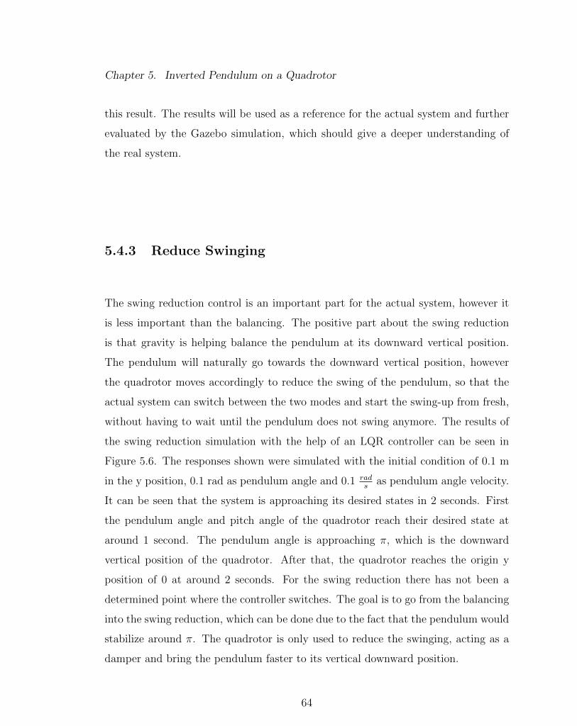
Chapter 5. Inverted Pendulum on a Quadrotor
this result. The results will be used as a reference for the actual system and further
evaluated by the Gazebo simulation, which should give a deeper understanding of
the real system.
5.4.3 Reduce Swinging
The swing reduction control is an important part for the actual system, however it
is less important than the balancing. The positive part about the swing reduction
is that gravity is helping balance the pendulum at its downward vertical position.
The pendulum will naturally go towards the downward vertical position, however
the quadrotor moves accordingly to reduce the swing of the pendulum, so that the
actual system can switch between the two modes and start the swing-up from fresh,
without having to wait until the pendulum does not swing anymore. The results of
the swing reduction simulation with the help of an LQR controller can be seen in
Figure 5.6. The responses shown were simulated with the initial condition of 0.1 m
in the y position, 0.1 rad as pendulum angle and 0.1 rads
as pendulum angle velocity.
It can be seen that the system is approaching its desired states in 2 seconds. First
the pendulum angle and pitch angle of the quadrotor reach their desired state at
around 1 second. The pendulum angle is approaching π, which is the downward
vertical position of the quadrotor. After that, the quadrotor reaches the origin y
position of 0 at around 2 seconds. For the swing reduction there has not been a
determined point where the controller switches. The goal is to go from the balancing
into the swing reduction, which can be done due to the fact that the pendulum would
stabilize around π. The quadrotor is only used to reduce the swinging, acting as a
damper and bring the pendulum faster to its vertical downward position.
64

Chapter 5. Inverted Pendulum on a Quadrotor
0 1 2 3 4 5
Time(sec)
0
0.05
0.1P
ositi
on(m
)
Swing Reduction Response with LQR Control
y
0 1 2 3 4 5
Time(sec)
-5
0
5
Ang
le(r
ad)
φ
0 1 2 3 4 5
Time(sec)
3.1
3.2
3.3
Ang
le(r
ad)
α
Figure 5.6: Responses of the states to reducing the swing of the pendulum. Firstgraph shows the y position of the quadrotor, second graph shows the pitch angle ofthe quadrotor and the last graph shows the pendulum angle.
5.5 Gazebo
For the Gazebo simulation, the existing package rotors simulator has been used
to model the quadrotor to have a model with exact characteristics and inertias [43].
The pendulum, its arm and a counterweight has been added to the model using
xacro programming language, which is used to build Gazebo models. The exact
measurements and inertia’s for the three parts have been calculated and used to
create a model which is as close as possible to the real system. The controllers have
been developed from zero and can be seen in Appendix B. The attitude control is
represented by the Roll pendulum, Pitch pendulum and Yaw pendulum notes seen
65

Chapter 5. Inverted Pendulum on a Quadrotor
in the figure. For the position control the Altitude pendulum node is holding the
quadrotor at 1m height at any point of the simulation and the X pendulum and
Y pendulum generate an input for the attitude controller so that the pendulum
stays at the origin at any point the position control is enabled. The input goes into
the Transform node, which secures that even at a heading change the desired roll and
pitch angles are achieved. For the linear swing-up control, the EnergieControlLateral
node generates the input for the acceleration controller which controls the roll angle
of the quadrotor. The LQR Lateral node balances the pendulum when it is at its
upward vertical position. The EnergieControlLateral generates the control input
heading acceleration control, which switches to the LQR Rotational control when
the pendulum angle is close to zero. The LQR Reduce Swing control is enabled to
reduce the pendulum swing at the hovering position. All these inputs go into the
Motor Commands pendulum node which is the decision control. It makes sure that
the right topics are used to generate the rotational speeds. The flight modes can be
switched with an XBox controller which is connected via the joy node. When the
rotational speeds are generated, they are published to the gazebo model.
The results for the linear swing-up and balancing can be seen in Figure 5.7. The
first graph shows the position results for the experiment, the second subplot shows
the quadrotor angles and the last shows the pendulum angle. The solid line shows
the swing-up maneuver and the dotted lines show the LQR control. At the beginning
the roll angle goes from -35 to 50 degrees, which is an aggressive maneuver to get
the pendulum swinging. At around 1.4 seconds the pendulum is close to the upward
vertical position, where it switches to the LQR controller. During the whole process
the pendulum is only swinging once, before it gets to the second swing where it is
getting close enough to switch to balancing control. During the LQR control roll
is much smoother, and when the pendulum is stable it slowly brings the quadrotor
with the balanced pendulum to the origin. A time sequence of the experiment can
be seen in Appendix C in Figure C.1. It shows a short part of the movie that has
66

Chapter 5. Inverted Pendulum on a Quadrotor
been recorded during the simulation. This experiment has also been used for the
graphs which are shown here.
0 1 2 3 4 5 6
-2
0
2Position of Quad
X
Y
Z
0 1 2 3 4 5 6
-2
0
2Rotation of Quad
φ
θ
ψ
0 1 2 3 4 5 6
0
5
10Pendulum Angle
α
Figure 5.7: Translational position and rotational angle of quadrotor and pendulumfor linear swing-up and balancing.
The results for the rotational swing-up and balancing are shown in 5.8. It should
be noticed that the position during the rotation of the quadrotor is fluctuating more
than during the linear control. It is getting smoother for the LQR balancing control.
The quadrotor is rotating aggressively during the swing-up and continues rotating
during the balancing control. This is because the heading control is the weakest
control input. The quadrotor is able to balance the pendulum, however it is not
able to hold its yaw at 0 degrees, which acts as a desired value for the controller.
The pendulum needs a little more time and swing before the controller switches. It
needs three swings, before the fourth swing brings the pendulum close enough to the
67
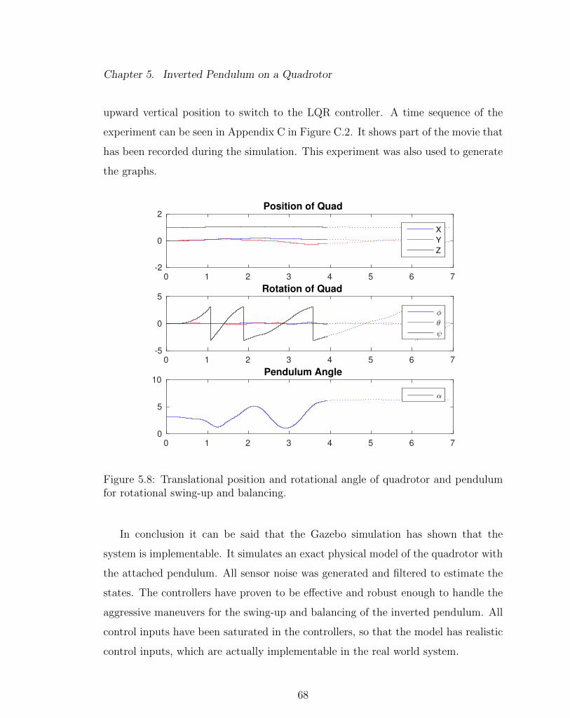
Chapter 5. Inverted Pendulum on a Quadrotor
upward vertical position to switch to the LQR controller. A time sequence of the
experiment can be seen in Appendix C in Figure C.2. It shows part of the movie that
has been recorded during the simulation. This experiment was also used to generate
the graphs.
0 1 2 3 4 5 6 7
-2
0
2Position of Quad
X
Y
Z
0 1 2 3 4 5 6 7
-5
0
5Rotation of Quad
φ
θ
ψ
0 1 2 3 4 5 6 7
0
5
10Pendulum Angle
α
Figure 5.8: Translational position and rotational angle of quadrotor and pendulumfor rotational swing-up and balancing.
In conclusion it can be said that the Gazebo simulation has shown that the
system is implementable. It simulates an exact physical model of the quadrotor with
the attached pendulum. All sensor noise was generated and filtered to estimate the
states. The controllers have proven to be effective and robust enough to handle the
aggressive maneuvers for the swing-up and balancing of the inverted pendulum. All
control inputs have been saturated in the controllers, so that the model has realistic
control inputs, which are actually implementable in the real world system.
68

Chapter 5. Inverted Pendulum on a Quadrotor
5.6 Implementation
For the implementation, the two different quadrotor models have been tested with the
pendulum attached to it. After testing both models, the QAV250 frame was used due
to its advantage of Oneshot125 capability, payload advantage and maneuverability.
Custom parts have been developed for the quadrotor to increase its visibility by
Vicon and be able to attach the pendulum. The pendulum itself has been build out
of carbon fiber rods, a ball bearing and custom designed and printed parts. The
system with its custom parts can be seen in Figure 5.9. The pendulum has been
designed lightweight by using carbon fiber. The total attachments added 39g to the
810g quadrotor, so that the total system had a weight of 849g with the battery. The
length of the pendulum is 75cm. It is important to notice that the MARHES testbed
area is 2.5m high, so the quadrotor has to be able to hold the altitude since there
is not a lot of room in the vertical direction before the ground or ceiling is touched.
It was not necessary to add a counterweight. The battery had been repositioned
towards the negative on the body x-axis to create a moment around the quadrotor
body origin and counteract the moment that is created by the pendulum. As a result
the battery is bringing the COM back to the origin, for the case that the pendulum is
not swinging. It is known that the COM is moving along the x-axis as the pendulum
is rotating, however the quadrotor LL attitude control is robust enough to take this
into account.
For the implementation a position control has been implemented for the takeoff,
landing and hovering position hold. The linear controllers send velocities to the
quadrotor. For the energy and LQR controllers the y or ψ reference will replace the
position control references. However, the other states will still be controlled by the
position controllers. The digital switch is controlled manually by Xbox controller
which is implemented in the ROS framework and is connected to the control nodes.
The rospackage used for the controller is joy.
69
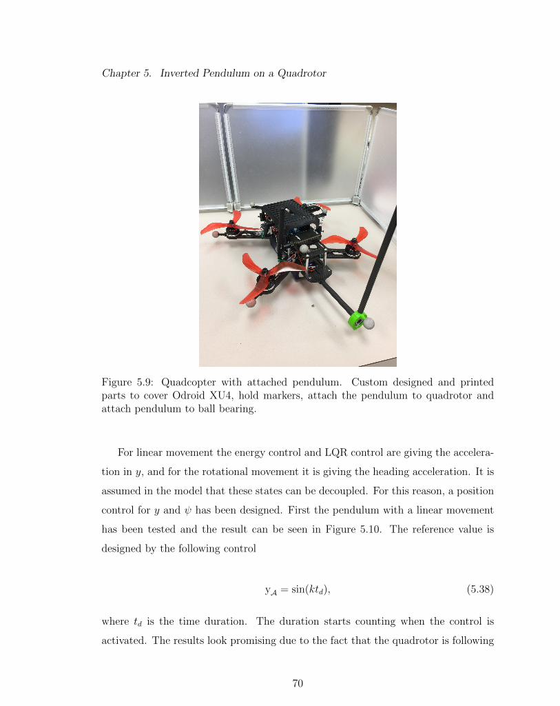
Chapter 5. Inverted Pendulum on a Quadrotor
Figure 5.9: Quadcopter with attached pendulum. Custom designed and printedparts to cover Odroid XU4, hold markers, attach the pendulum to quadrotor andattach pendulum to ball bearing.
For linear movement the energy control and LQR control are giving the accelera-
tion in y, and for the rotational movement it is giving the heading acceleration. It is
assumed in the model that these states can be decoupled. For this reason, a position
control for y and ψ has been designed. First the pendulum with a linear movement
has been tested and the result can be seen in Figure 5.10. The reference value is
designed by the following control
yA = sin(ktd), (5.38)
where td is the time duration. The duration starts counting when the control is
activated. The results look promising due to the fact that the quadrotor is following
70

Chapter 5. Inverted Pendulum on a Quadrotor
the reference position. More importantly it can be noticed that x, z and ψ are stable
and stay close to their references. The pendulum is moving as a result of the linear
motion. However, since the controller does not try to get it to the upward vertical
position it stays around its downward vertical equilibrium point. This result looks
promising and gives confidence to take the next step.
Figure 5.10: Linear position control of quadrotor with pendulum attached.
After testing the linear movement with the quadrotor attached, the rotational
movement has been tested. Similarly to the linear position generation a position has
been generated for the ψ position. The position has been generated using
71

Chapter 5. Inverted Pendulum on a Quadrotor
ψ = 1.5 ∗ sin(ktd), (5.39)
.
The position is amplified by 1.5 due to experimenting and the engineering judg-
ment achieved by the tests. Figure 5.11 shows the results of the test. It can be seen
that x and y are moving when the quadrotor is rotating its heading. The quadrotor
is able to hover around the origin, however its reaction could be improved. The
altitude is stable around 1m. The pendulum angle is moving due to the rotation.
Figure 5.11: Rotational position control of quadrotor with pendulum attached.
The results of the linear and rotational position control give promising results.
72

Chapter 5. Inverted Pendulum on a Quadrotor
It has been shown that the states can be decoupled. Improvements could be made
in the x and y position when the quadrotor is rotating. It can be seen that the
quadrotor has inputs to the pendulum, however the pendulum is light enough to not
affect the quadrotor. The LL and HL controllers are robust enough to counteract
the change in COM during the movement.
73

Chapter 6
Conclusions, Contributions and
Improvements
6.1 Conclusions
In this thesis a ROS based framework for quadrotors at the MARHES lab has been
developed. The framework makes the UAV interface user friendly and existing at-
titude and position controllers can be used by the users. Additionally ROS makes
it possible to control multiple UAVs at once. This framework is state of the art for
robotics laboratories and helps to use the aerial vehicles for different applications.
The different hardware and software used for this thesis has been explained in
detail. The quadrotor model has been derived using Newton-Euler approach with
rigid body assumptions. The system architecture shows the implementation of the
framework on two quadrotors with different FC. It demonstrates that even though
the quadrotors have different LL controllers, they can be controlled similarly on the
HL side, which simplifies the implementation of them in a network.
74

Chapter 6. Conclusions, Contributions and Improvements
Two applications are explained that were used to demonstrate the flexibility of
the quadrotor. The MAST and ASAP project make use of the new framework. For
the MAST project a linear position controller has been developed and implemented.
Different velocity estimators have been tested and implemented, the best performing
estimator is used for the position control. A demo has been designed and explained
where the quadrotor hops between different ground vehicles to extract data from
them. For the ASAP project a trajectory generation and implementation algorithm
has been tested and documented. The implementation architecture shows the use of
Matlab in the framework. Tests for an open loop reachability analysis are discussed.
A framework for a pendulum on a quadrotor is presented. It explains the possibil-
ity of swinging-up and balancing a rotational and linear pendulum with a quadrotor
as the actuator. The complete model is derived using Lagrangian. Control algorithms
for the hybrid controller have been developed and tested for stability. First Matlab
is used to calculate the LQR gain matrices which are used in the Gazebo simulation
to demonstrate the system. First steps and tests for a real system implementation
are documented.
6.2 Contributions
The main contributions of this thesis are
• ROS UAV Framework: This thesis developed a framework for on-board mi-
croprocessors on quadrotors which use Robot Operating System. They get
position data from Vicon and it is possible to control them with standard ROS
messages. Additionally it is possible to communicate with them on a ground
station using ROS and/or Matlab’s Robotic Toolbox.
• Architecture: The system is explaining the implementation architecture in de-
75

Chapter 6. Conclusions, Contributions and Improvements
tail. It can be seen that the HL side is similar, even though the LL control side
uses different FC.
• Position Control: A linear position control is implemented. It shows good
results, whereas the focus was on stable flying around the desired position for
the MAST project. This position control will benefit the implementation of
optical communication devices on the quadrotor.
• Trajectory Tracking: Trajectory tracking in the framework of the ASAP project
is implemented. It generates smooth flight paths using 3rd order polynomials
in Matlab. The Matlab Robotics Toolbox has been used to send the trajectory
coefficients to the quadrotor.
• Pendulum on a Quadrotor: A framework for an off-centered pendulum on a
quadrotor has been developed. The model has been derived and a promising
control strategy developed. The simulations show promising results and the
implementation has been discussed.
6.3 Improvements
The quadrotors are limited by the Vicon area that is provided. The framework has
the possibility to switch Vicon position feedback with GPS feedback, so that it is
possible to go outdoors. This would also make it possible to add more agents to the
network of UAV’s.
The LL controllers present some limitations by themselves. It is possible to con-
trol both quadrotors that were developed in the framework via direct motor control.
This could improve the responsiveness and overall output of the system. Much re-
search has been done in ESC protocols. Being able to switch to faster protocols
(Oneshot42, Multishot) or digital protocols (DSHOT150, DSHOT300, DSHOT600,
76
Chapter 6. Conclusions, Contributions and Improvements
DSHOT1200) could improve performance as well as reduce noise between the LL
controller and the ESC.
Different controllers could be implemented in the framework. The control inputs
to the framework could be changed and probably make the quadrotor faster, more
agile and more stable.
Cooperative applications and algorithms could be implemented to test the net-
work ability of the framework.
77

Appendices
A Graphs for Trajectory Tracking a Figure Eight 79
B Gazebo Simulation 84
C Picture Sequence of Gazebo Simulation 86
78

Appendix A
Graphs for Trajectory Tracking a
Figure Eight
This results of flying a figure eight trajectory have been documented here. The
quadrotor has been tested at different speeds. The different gains, k, control the
speed of the vehicle. The UAV has been tested for the gains 0.5,1.0,1.5 and 2.
The paragraphs show each position of the quadcopter at specific times and how it
performs against its reference.
79

Appendix A. Graphs for Trajectory Tracking a Figure Eight
Figure A.1: Position vs. time graphs for trajectory tracking figure eight with gaink=0.5
80

Appendix A. Graphs for Trajectory Tracking a Figure Eight
Figure A.2: Position vs. time graphs for trajectory tracking figure eight with gaink=1.0
81

Appendix A. Graphs for Trajectory Tracking a Figure Eight
Figure A.3: Position vs. time graphs for trajectory tracking figure eight with gaink=1.5
82

Appendix A. Graphs for Trajectory Tracking a Figure Eight
Figure A.4: Position vs. time graphs for trajectory tracking figure eight with gaink=2.0
83

Appendix B
Gazebo Simulation
The Gazebo simulation has been developed with the help of the rotors gazebo pack-
age developed by students from ETH-Zurich. This has the advantage that the hum-
mingbird quadrotors have exact characteristics, so that the simulation will be as
close as possible to the real world. The pendulum has been added to the quadrotor
with exact measurements and inertia’s. The controllers for every level have been
developed. The control tree can be seen in Figure B.1.
84
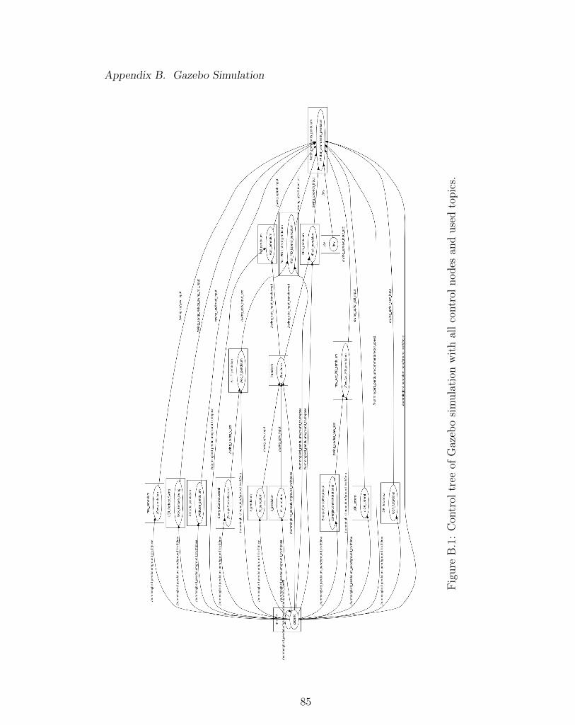
Appendix B. Gazebo Simulation
Fig
ure
B.1
:C
ontr
oltr
eeof
Gaz
ebo
sim
ula
tion
wit
hal
lco
ntr
olnodes
and
use
dto
pic
s.
85

Appendix C
Picture Sequence of Gazebo
Simulation
The picture sequences taken to display the swing-up and balancing control of the
pendulum has been developed using Gazebo and Matlab. First a video of the com-
plete simulation has been recorded. The video was cut into the rotational and linear
simulation. The video was imported into Matlab and separated into pictures. The
pictures have been converted into a sequence to show the process. The linear swing-
up and balancing can be seen in Figure C.1 and the rotational can be seen in C.2.
86

Appendix C. Picture Sequence of Gazebo Simulation
Figure C.1: Picture sequence of swing-up and balancing simulation the linear pen-dulum on a quadrotor in Gazebo.
87

Appendix C. Picture Sequence of Gazebo Simulation
Figure C.2: Picture sequence of swing-up and balancing simulation the rotationalpendulum on a quadrotor in Gazebo.
88

References
[1] “Documentation.” https://www.mathworks.com/help/robotics/examples/
exchange-data-with-ros-publishers-and-subscribers.html.
[2] G. Hoffmann, D. G. Rajnarayan, S. L. Waslander, D. Dostal, J. S. Jang, andC. J. Tomlin, “The stanford testbed of autonomous rotorcraft for multi agentcontrol (starmac),” in Digital Avionics Systems Conference, 2004. DASC 04.The 23rd, vol. 2, pp. 12–E, IEEE, 2004.
[3] N. Michael, D. Mellinger, Q. Lindsey, and V. Kumar, “The grasp multiple micro-uav testbed,” IEEE Robotics & Automation Magazine, vol. 17, no. 3, pp. 56–65,2010.
[4] M. Valenti, B. Bethke, D. Dale, A. Frank, J. McGrew, S. Ahrens, J. P. How,and J. Vian, “The mit indoor multi-vehicle flight testbed,” in Robotics andAutomation, 2007 IEEE International Conference on, pp. 2758–2759, IEEE,2007.
[5] S. Lupashin, A. Schollig, M. Hehn, and R. D’Andrea, “The flying machine arenaas of 2010,” in Robotics and Automation (ICRA), 2011 IEEE InternationalConference on, pp. 2970–2971, IEEE, 2011.
[6] L. R. Garcıa Carrillo, A. E. Dzul Lopez, R. Lozano, and C. Pegard, Modelingthe Quad-Rotor Mini-Rotorcraft, pp. 23–34. London: Springer London, 2013.
[7] S. Bouabdallah, A. Noth, and R. Siegwart, “Pid vs lq control techniquesapplied to an indoor micro quadrotor,” in Intelligent Robots and Systems,2004.(IROS 2004). Proceedings. 2004 IEEE/RSJ International Conference on,vol. 3, pp. 2451–2456, IEEE, 2004.
[8] T. Bresciani, “Modelling, identification and control of a quadrotor helicopter,”MSc Theses, 2008.
89

References
[9] H. Huang, G. M. Hoffmann, S. L. Waslander, and C. J. Tomlin, “Aerodynamicsand control of autonomous quadrotor helicopters in aggressive maneuvering,”in 2009 IEEE International Conference on Robotics and Automation, pp. 3277–3282, May 2009.
[10] D. Mellinger, N. Michael, and V. Kumar, “Trajectory generation and controlfor precise aggressive maneuvers with quadrotors,” The International Journalof Robotics Research, vol. 31, no. 5, pp. 664–674, 2012.
[11] P. J. Cruz Davalos, Real-time control architecture for a multi UAV test bed. PhDthesis, 2013.
[12] W. Neeley, Design and Development of a High-Performance Quadrotor ControlArchitecture Based on Feedback Linearization. PhD thesis, 2016.
[13] J. Boren and S. Cousins, “Exponential growth of ros [ros topics],” IEEE Robotics& Automation Magazine, vol. 18, no. 1, pp. 19–20, 2011.
[14] S. Cousins, B. Gerkey, K. Conley, and W. Garage, “Sharing software with ros[ros topics],” IEEE Robotics & Automation Magazine, vol. 17, no. 2, pp. 12–14,2010.
[15] S. Edwards and C. Lewis, “Ros-industrial: applying the robot operating sys-tem (ros) to industrial applications,” in IEEE Int. Conference on Robotics andAutomation, ECHORD Workshop, 2012.
[16] A. A. El-Badawy and M. A. Bakr, “Quadcopter aggressive maneuvers along sin-gular configurations: an energy-quaternion based approach,” Journal of ControlScience and Engineering, vol. 2016, p. 4, 2016.
[17] M. Achtelik, T. Bierling, J. Wang, L. Hocht, and F. Holzapfel, “Adaptive controlof a quadcopter in the presence of large/complete parameter uncertainties,”Infotech@ Aerospace, pp. 29–31, 2011.
[18] I. Palunko, P. Cruz, and R. Fierro, “Agile load transportation: Safe and efficientload manipulation with aerial robots,” IEEE Robotics & Automation Magazine,vol. 19, no. 3, pp. 69–79, 2012.
[19] P. J. Cruz and R. Fierro, “Towards optical wireless communications betweenmicro unmanned aerial and ground systems,” in Unmanned Aircraft Systems(ICUAS), 2015 International Conference on, pp. 669–676, IEEE, 2015.
[20] B. HomChaudhuri, A. P. Vinod, and M. M. Oishi, “Computation of forwardstochastic reach sets: Application to stochastic, dynamic obstacle avoidance,”in American Control Conference (ACC), 2017, pp. 4404–4411, IEEE, 2017.
90

References
[21] A. P. Vinod, B. Homchaudhuri, and M. M. Oishi, “Forward stochastic reacha-bility analysis for uncontrolled linear systems using fourier transforms,” in Pro-ceedings of the 20th International Conference on Hybrid Systems: Computationand Control, pp. 35–44, ACM, 2017.
[22] J. Aracil, J. Acosta, and F. Gordillo, “A nonlinear hybrid controller for swinging-up and stabilizing the furuta pendulum,” Control Engineering Practice, vol. 21,no. 8, pp. 989–993, 2013.
[23] K. J. Astrom and K. Furuta, “Swinging up a pendulum by energy control,”Automatica, vol. 36, no. 2, pp. 287–295, 2000.
[24] V. Sukontanakarn and M. Parnichkun, “Real-time optimal control for rotaryinverted pendulum,” American journal of applied sciences, vol. 6, no. 6, p. 1106,2009.
[25] S. Awtar, N. King, T. Allen, I. Bang, M. Hagan, D. Skidmore, and K. Craig, “In-verted pendulum systems: rotary and arm-driven-a mechatronic system designcase study,” Mechatronics, vol. 12, no. 2, pp. 357–370, 2002.
[26] M. Hehn and R. D’Andrea, “A flying inverted pendulum,” in Robotics and Au-tomation (ICRA), 2011 IEEE International Conference on, pp. 763–770, IEEE,2011.
[27] D. Brescianini, M. Hehn, and R. D’Andrea, “Quadrocopter pole acrobatics,” in2013 IEEE/RSJ International Conference on Intelligent Robots and Systems,pp. 3472–3479, IEEE, 2013.
[28] “Turtlebot2.” http://www.turtlebot.com/turtlebot2/.
[29] “Pioneer 3-at.” http://www.mobilerobots.com/ResearchRobots/P3AT.aspx.
[30] “4x4 monster pick-up txt-1.” http://www.tamiya.com/english/products/
58280txt_1/txt_1.htm.
[31] “Posts about octoroach on robotics.” https://walterfarah.wordpress.com/
tag/octoroach/.
[32] “miniroach.” http://marhes.unm.edu/?page_id=1206.
[33] “Asctec hummingbird /// research and development uas for swarming andcontrol theory..” http://www.asctec.de/en/uav-uas-drones-rpas-roav/
asctec-hummingbird/.
91

References
[34] “Baxter collaborative robots for industrial automation.” http://www.
rethinkrobotics.com/baxter/.
[35] Vicon, “Motion capture systems.” https://www.vicon.com/.
[36] “Odroid — hardkernel.” http://www.hardkernel.com/main/products/prdt_
info.php.
[37] “Jetson tk1 embedded developer kit from nvidia.” http://www.nvidia.com/
object/jetson-tk1-embedded-dev-kit.html.
[38] A. Industries, “Raspberry pi zero w.” https://www.adafruit.com/product/
3400.
[39] F. Kendoul, “Survey of advances in guidance, navigation, and control of un-manned rotorcraft systems,” Journal of Field Robotics, vol. 29, no. 2, pp. 315–378, 2012.
[40] “Pixracer autopilot.” https://pixhawk.org/modules/pixracer.
[41] “Wiki.” http://wiki.ros.org/ROS/Introduction.
[42] Osrf, “Why gazebo?.” http://gazebosim.org/.
[43] F. Furrer, M. Burri, M. Achtelik, and R. Siegwart, Robot Operating System(ROS): The Complete Reference (Volume 1), ch. RotorS—A Modular GazeboMAV Simulator Framework, pp. 595–625. Cham: Springer International Pub-lishing, 2016.
[44] T. Luukkonen, “Modelling and control of quadcopter,” Independent researchproject in applied mathematics, Espoo, 2011.
[45] R. Mahony, V. Kumar, and P. Corke, “Multirotor aerial vehicles,” IEEERobotics and Automation magazine, vol. 20, no. 32, 2012.
[46] M. K. Habib, W. G. A. Abdelaal, M. S. Saad, et al., “Dynamic modeling andcontrol of a quadrotor using linear and nonlinear approaches,” 2014.
[47] J. Li and Y. Li, “Dynamic analysis and pid control for a quadrotor,” in Mecha-tronics and Automation (ICMA), 2011 International Conference on, pp. 573–578, IEEE, 2011.
[48] M. A. Al-Alaoui, “Al-alaoui operator and the new transformation polynomialsfor discretization of analogue systems,” Electrical Engineering, vol. 90, no. 6,pp. 455–467, 2008.
92

References
[49] R. P. K. Jain, “Transportation of cable suspended load using unmanned aerialvehicles: A real-time model predictive control approach,” 2015.
[50] P. Kotaru, G. Wu, and K. Sreenath, “Dynamics and control of a quadrotor witha payload suspended through an elastic cable,” in American Control Conference(ACC), to appear, 2017.
[51] K. J. Astrom, “Hybrid control of inverted pendulums,” in Learning, control andhybrid systems, pp. 150–163, Springer, 1999.
[52] R. Fierro, F. L. Lewis, and A. Lowe, “Hybrid control for a class of underactuatedmechanical systems,” IEEE Transactions on Systems, Man, and Cybernetics-Part A: Systems and Humans, vol. 29, no. 6, pp. 649–654, 1999.
93