Root-Locus Analysiseng.sut.ac.th/me/meold/3_2551/425308/ACS41.pdfSeven Steps to Sketching a...
19
Root-Locus Analysis Chapter IV Root-Locus Analysis 2 Introduction 3 Introduction video camera system 4 Introduction video camera system Pole location as a function of gain for the system
Transcript of Root-Locus Analysiseng.sut.ac.th/me/meold/3_2551/425308/ACS41.pdfSeven Steps to Sketching a...
Root-Locus AnalysisChapter IV
Root-Locus Analysis
2
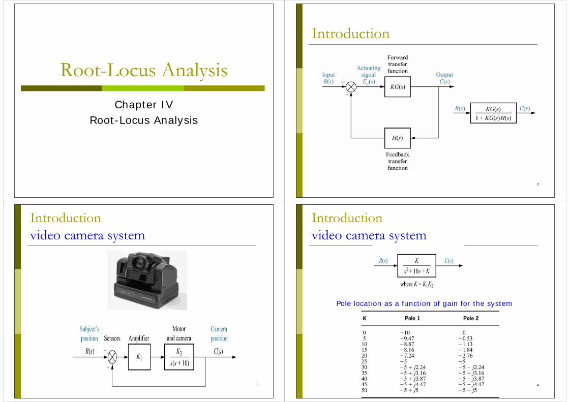
Introduction
3
Introductionvideo camera system
4
Introductionvideo camera system
Pole location as a function of gain for the system
5
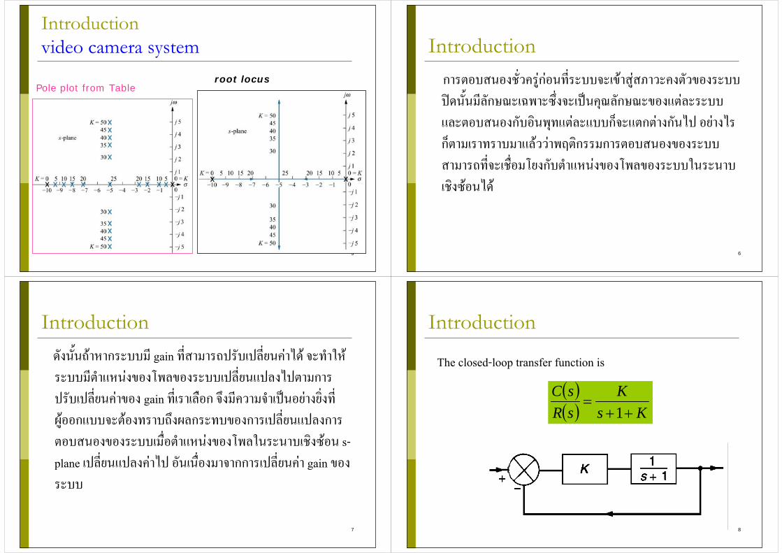
Introductionvideo camera system
Pole plot from Table root locus
6
Introductionการตอบสนองชั่วครูกอนที่ระบบจะเขาสูสภาวะคงตัวของระบบปดนั้นมีลักษณะเฉพาะซึ่งจะเปนคุณลักษณะของแตละระบบและตอบสนองกับอินพุทแตละแบบก็จะแตกตางกันไป อยางไรก็ตามเราทราบมาแลววาพฤติกรรมการตอบสนองของระบบสามารถที่จะเชือ่มโยงกับตําแหนงของโพลของระบบในระนาบเชิงซอนได
7
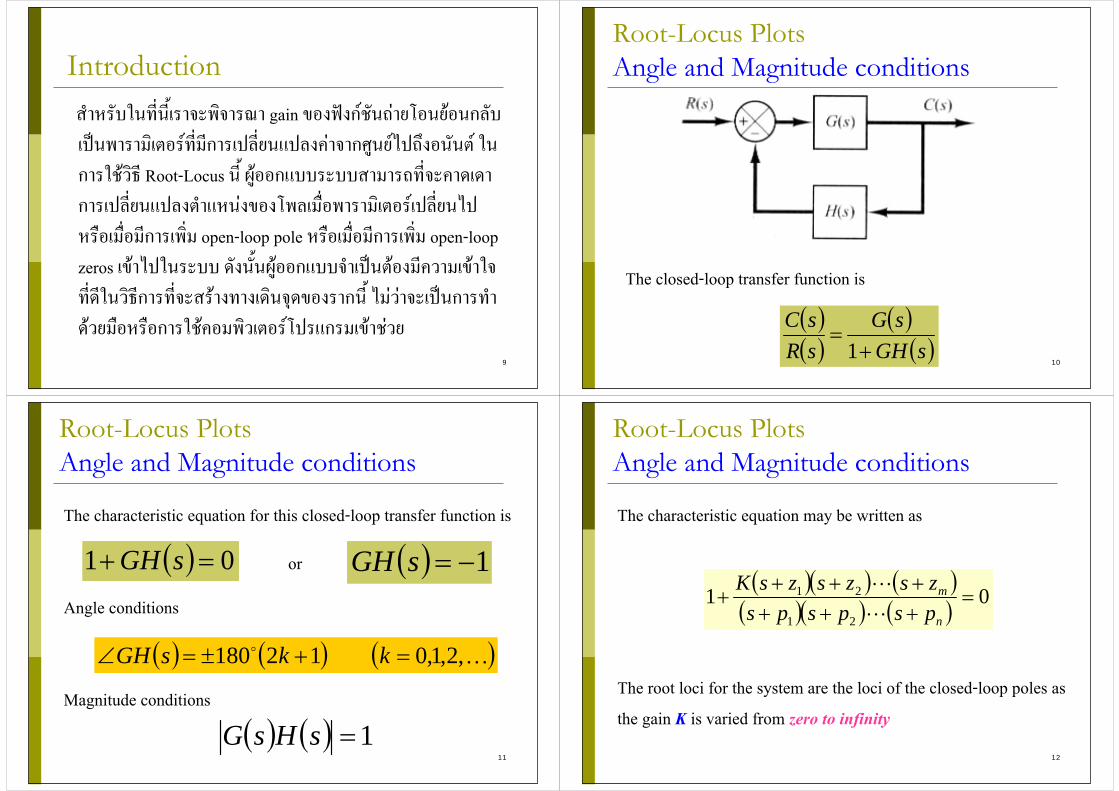
Introductionดังนัน้ถาหากระบบมี gain ที่สามารถปรับเปลี่ยนคาได จะทําใหระบบมีตําแหนงของโพลของระบบเปลี่ยนแปลงไปตามการปรับเปลี่ยนคาของ gain ที่เราเลือก จงึมีความจําเปนอยางยิ่งที่ผูออกแบบจะตองทราบถึงผลกระทบของการเปลี่ยนแปลงการตอบสนองของระบบเมื่อตําแหนงของโพลในระนาบเชิงซอน s-plane เปลี่ยนแปลงคาไป อันเนือ่งมาจากการเปลี่ยนคา gain ของระบบ
8
Introduction
( )( ) Ks
KsRsC
++=
1
The closed-loop transfer function is
9
Introductionสําหรับในที่นีเ้ราจะพจิารณา gain ของฟงกชันถายโอนยอนกลับเปนพารามิเตอรที่มีการเปลี่ยนแปลงคาจากศนูยไปถึงอนนัต ในการใชวิธี Root-Locus นี้ ผูออกแบบระบบสามารถที่จะคาดเดาการเปลี่ยนแปลงตําแหนงของโพลเมื่อพารามิเตอรเปลี่ยนไป หรือเมื่อมกีารเพิ่ม open-loop pole หรือเมือ่มีการเพิ่ม open-loop zeros เขาไปในระบบ ดังนัน้ผูออกแบบจําเปนตองมีความเขาใจที่ดีในวธิกีารที่จะสรางทางเดินจุดของรากนี้ ไมวาจะเปนการทําดวยมือหรือการใชคอมพิวเตอรโปรแกรมเขาชวย
10
Root-Locus PlotsAngle and Magnitude conditions
( )( )
( )( )sGH
sGsRsC
+=
1
The closed-loop transfer function is
11
Root-Locus PlotsAngle and Magnitude conditions
( ) 01 =+ sGH ( ) 1−=sGH
( ) ( ) ( )…,2,1,0 12180 =+±=∠ kksGH
The characteristic equation for this closed-loop transfer function is
Angle conditions
Magnitude conditions( ) ( ) 1=sHsG
or
12
Root-Locus PlotsAngle and Magnitude conditions
( )( ) ( )( )( ) ( ) 01
21
21 =++++++
+n
m
pspspszszszsK
The characteristic equation may be written as
The root loci for the system are the loci of the closed-loop poles as the gain K is varied from zero to infinity
13
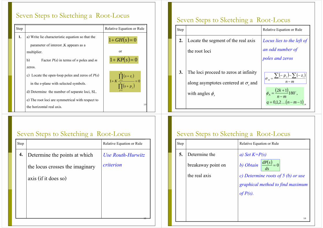
Seven Steps to Sketching a Root-Locus
or
a) Write lie characteristic equation so that theparameter of interest ,K appears as a
multiplier.b) Factor P(s) in terms of n poles and m zeros. c) Locate the open-loop poles and zeros of P(s)
in the s-plane with selected symbols.d) Determine the number of separate loci, SL.e) The root loci are symmetrical with respect to the horizontal real axis.
1.Relative Equation or RuleStep
( ) 01 =+ sGH
( ) 01 =+ sKP
( )
( )01
1
1 =+
++
∏
∏
=
=n
jj
m
ii
ps
zsK
14
Seven Steps to Sketching a Root-Locus
Locus lies to the left of an odd number of poles and zeros
Locate the segment of the real axisthe root loci
The loci proceed to zeros at infinity along asymptotes centered at σA and with angles φA
2.
3.
Relative Equation or RuleStep
( ) ( )mn
zp ijA −
−−−= ∑ ∑σ
( )
( )12,1,0
,18012
−−=−+
=
mnqmn
kA
…
φ
15
Seven Steps to Sketching a Root-Locus
Use Routh-Hurwitz criterion
Determine the points at whichthe locus crosses the imaginary axis (if it does so)
4.Relative Equation or RuleStep
16
Seven Steps to Sketching a Root-Locus
a) Set K=P(s)b) Obtainc) Determine roots of 5 (b) or use graphical method to find maximum of P(s).
Determine the breakaway point onthe real axis
5.Relative Equation or RuleStep
( ) 0=ds
sdP
17
Seven Steps to Sketching a Root-Locus
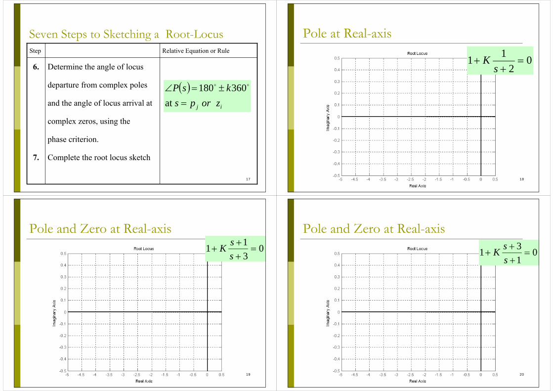
Determine the angle of locus departure from complex poles and the angle of locus arrival atcomplex zeros, using thephase criterion.Complete the root locus sketch
6.
7.
Relative Equation or RuleStep
( )ij zorps
ksP at
360180
=±=∠
18
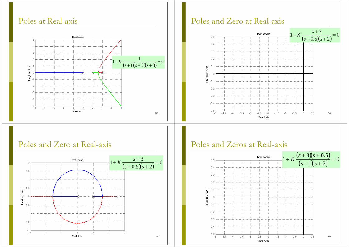
Pole at Real-axis
02
11 =+
+s
K
19
Pole and Zero at Real-axis0
311 =
++
+ssK
20
Pole and Zero at Real-axis
0131 =
++
+ssK
21
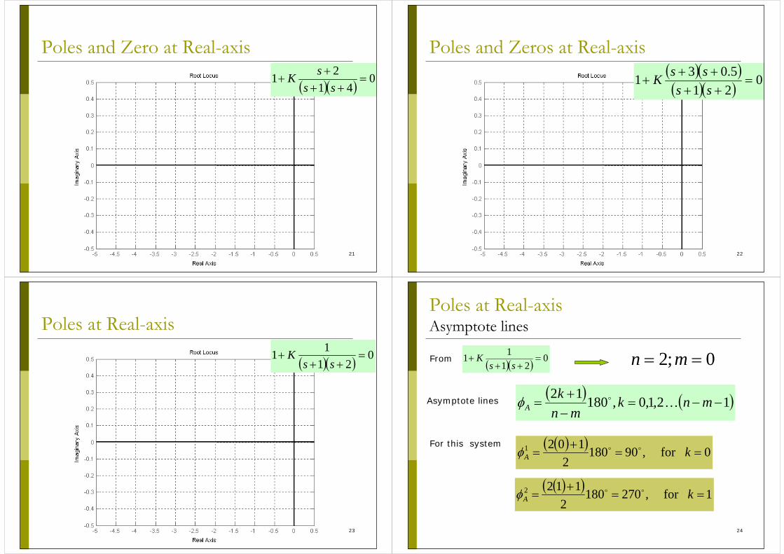
Poles and Zero at Real-axis
( )( ) 041
21 =++
++
sssK
22
Poles and Zeros at Real-axis( )( )( )( ) 0
215.031 =
++++
+ss
ssK
23
Poles at Real-axis
( )( ) 021
11 =++
+ss
K
24
Poles at Real-axisAsymptote lines
( )( ) 021
11 =++
+ss
K 0;2 == mn
( ) ( )12,1,0,18012−−=
−+
= mnkmn
kA …φAsymptote lines
From
( )( ) 0for ,901802
1021 ==+
= kAφ
( )( ) 1for ,2701802
1122 ==+
= kAφ
For this system
25
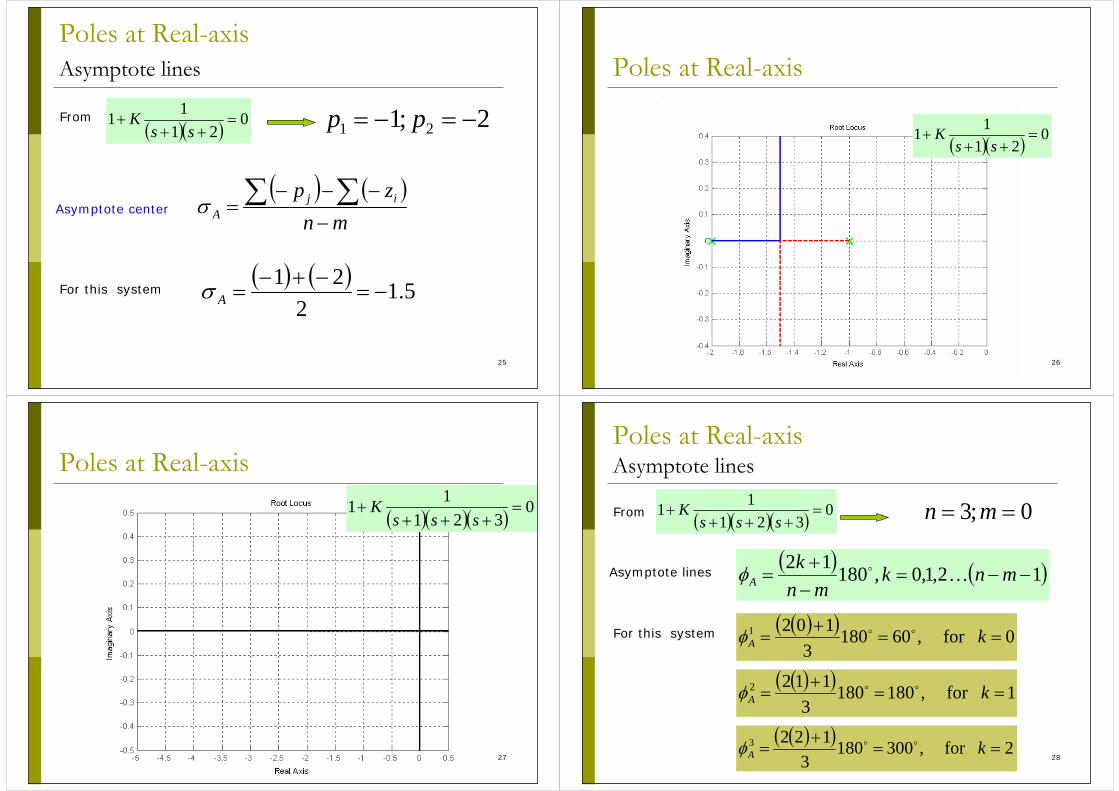
Poles at Real-axisAsymptote lines
( ) ( )mn
zp ijA −
−−−= ∑ ∑σ
( )( ) 021
11 =++
+ss
K 2;1 21 −=−= ppFrom
( ) ( ) 5.12
21−=
−+−=AσFor this system
Asymptote center
26
Poles at Real-axis
( )( ) 021
11 =++
+ss
K
27
Poles at Real-axis
( )( )( ) 0321
11 =+++
+sss
K
28
Poles at Real-axisAsymptote lines
( )( )( ) 0321
11 =+++
+sss
K 0;3 == mn
( ) ( )12,1,0,18012−−=
−+
= mnkmn
kA …φAsymptote lines
From
( )( ) 0for ,601803
1021 ==+
= kAφ
( )( ) 1for ,1801803
1122 ==+
= kAφ
For this system
( )( ) 2for ,3001803
1223 ==+
= kAφ
29
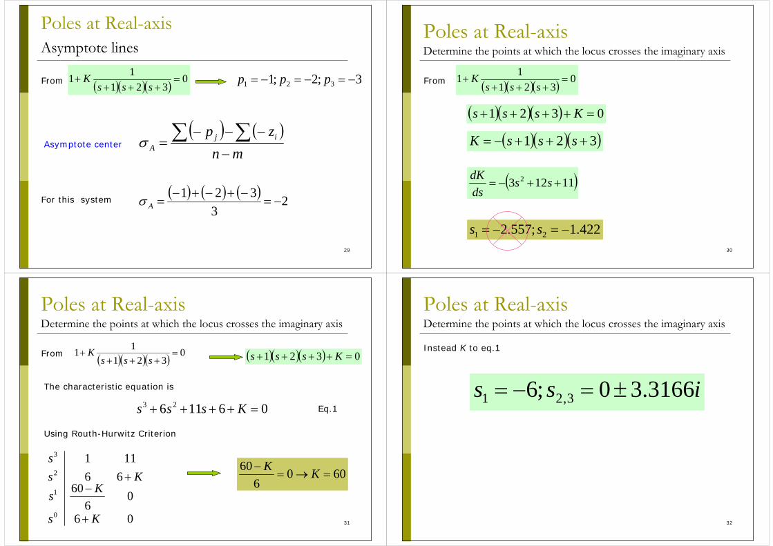
Poles at Real-axisAsymptote lines
( ) ( )mn
zp ijA −
−−−= ∑ ∑σ
( )( )( ) 0321
11 =+++
+sss
K 3;2;1 321 −=−=−= pppFrom
( ) ( ) ( ) 23
321−=
−+−+−=AσFor this system
Asymptote center
30
Poles at Real-axisDetermine the points at which the locus crosses the imaginary axis
( )( )( ) 0321 =++++ Ksss
( )( )( )321 +++−= sssK
( )11123 2 ++−= ssdsdK
( )( )( ) 0321
11 =+++
+sss
KFrom
422.1;557.2 21 −=−= ss
31
Poles at Real-axisDetermine the points at which the locus crosses the imaginary axis
( )( )( ) 0321 =++++ Ksss
06116 23 =++++ Ksss
06
06
6066
111
0
1
2
3
Ks
KsKs
s
+
−+
( )( )( ) 0321
11 =+++
+sss
KFrom
The characteristic equation is
Using Routh-Hurwitz Criterion
6006
60=→=
− KK
Eq.1
32
Poles at Real-axisDetermine the points at which the locus crosses the imaginary axis
Instead K to eq.1
iss 3166.30;6 3,21 ±=−=
33
Poles at Real-axis
( )( )( ) 0321
11 =+++
+sss
K
34
Poles and Zero at Real-axis
( )( ) 025.0
31 =++
++
sssK
35
Poles and Zero at Real-axis
( )( ) 025.0
31 =++
++
sssK
36
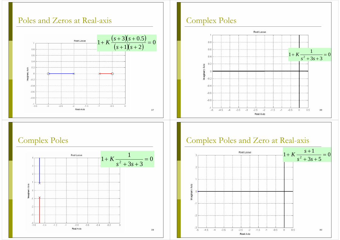
Poles and Zeros at Real-axis( )( )( )( ) 0
215.031 =
++++
+ss
ssK
37
Poles and Zeros at Real-axis
( )( )( )( ) 0
215.031 =
++++
+ss
ssK
38
Complex Poles
033
11 2 =++
+ss
K
39
Complex Poles
033
11 2 =++
+ss
K
40
Complex Poles and Zero at Real-axis0
5311 2 =++
++
sssK
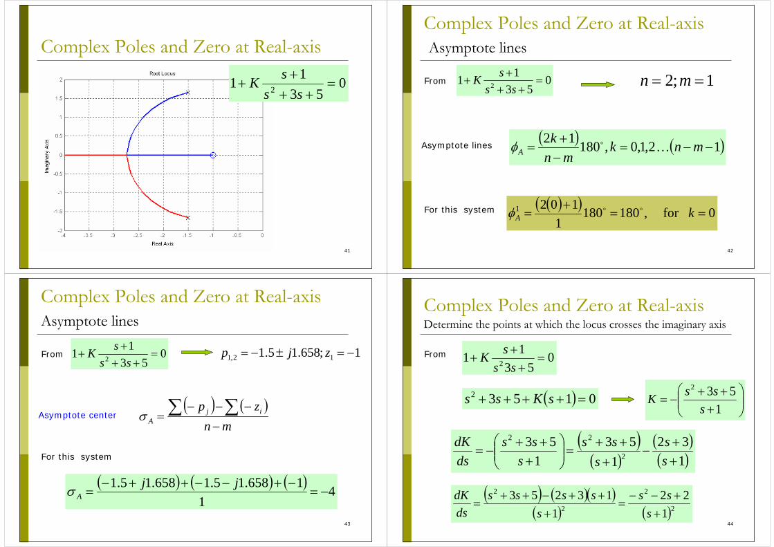
41
Complex Poles and Zero at Real-axis
053
11 2 =++
++
sssK
42
Complex Poles and Zero at Real-axis Asymptote lines
053
11 2 =++
++
sssK 1;2 == mn
( ) ( )12,1,0,18012−−=
−+
= mnkmn
kA …φAsymptote lines
From
( )( ) 0for ,1801801
1021 ==+
= kAφFor this system
43
Complex Poles and Zero at Real-axis Asymptote lines
( ) ( )mn
zp ijA −
−−−= ∑ ∑σ
053
11 2 =++
++
sssK 1;658.15.1 12,1 −=±−= zjpFrom
Asymptote center
( ) ( ) ( ) 41
1658.15.1658.15.1−=
−+−−++−=
jjAσ
For this system
44
Complex Poles and Zero at Real-axisDetermine the points at which the locus crosses the imaginary axis
( ) 01532 =++++ sKss ⎟⎟⎠
⎞⎜⎜⎝
⎛+++
−=1
532
sssK
053
11 2 =+
++
sssKFrom
( )( )
( )( )1
321
531
532
22
++
−+
++=⎟⎟
⎠
⎞⎜⎜⎝
⎛+++
−=ss
sss
sss
dsdK
( ) ( )( )( ) ( )2
2
2
2
122
113253
++−−
=+
++−++=
sss
sssss
dsdK
45
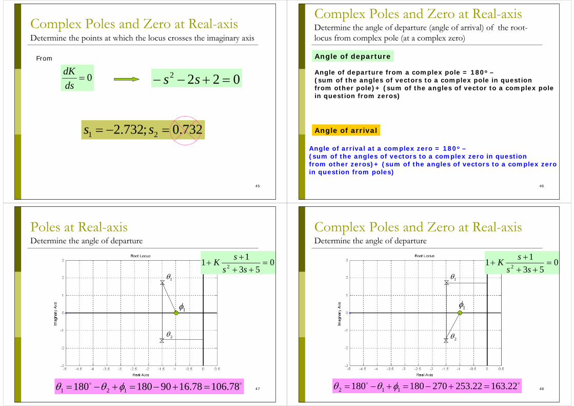
Complex Poles and Zero at Real-axisDetermine the points at which the locus crosses the imaginary axis
0=dsdK
0222 =+−− ss
732.0;732.2 21 =−= ss
From
46
Complex Poles and Zero at Real-axis Determine the angle of departure (angle of arrival) of the root-locus from complex pole (at a complex zero)
Angle of departure
Angle of departure from a complex pole = 180o –(sum of the angles of vectors to a complex pole in question from other pole)+ (sum of the angles of vector to a complex polein question from zeros)
Angle of arrival
Angle of arrival at a complex zero = 180o –(sum of the angles of vectors to a complex zero in question from other zeros)+ (sum of the angles of vectors to a complex zeroin question from poles)
47
Poles at Real-axisDetermine the angle of departure
053
11 2 =++
++
sssK
78.10678.1690180180 121 =+−=+−= φθθ
2θ
1φ
1θ
48
Complex Poles and Zero at Real-axis Determine the angle of departure
053
11 2 =++
++
sssK
22.16322.253270180180 112 =+−=+−= φθθ
2θ
1φ
1θ
49
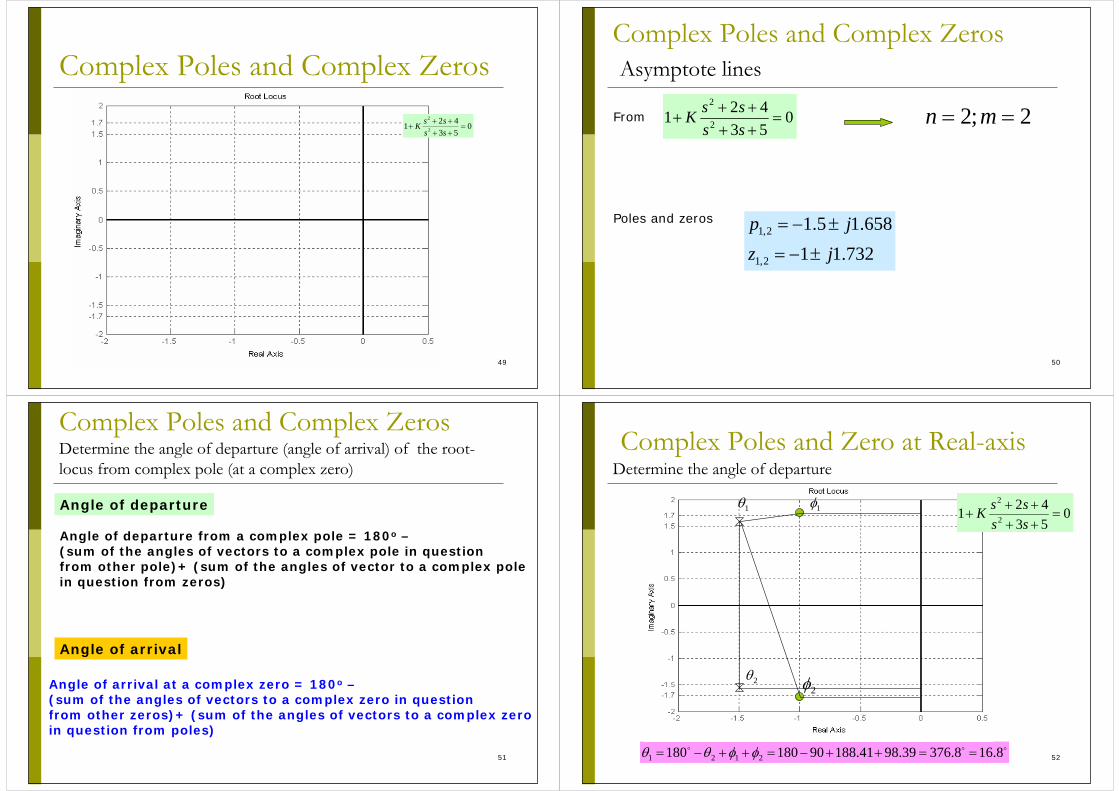
Complex Poles and Complex Zeros
053421 2
2
=++++
+ssssK
50
Complex Poles and Complex Zeros Asymptote lines
053421 2
2
=++++
+ssssK 2;2 == mnFrom
732.11658.15.1
2,1
2,1
jzjp
±−=
±−=Poles and zeros
51
Complex Poles and Complex Zeros Determine the angle of departure (angle of arrival) of the root-locus from complex pole (at a complex zero)
Angle of departure
Angle of departure from a complex pole = 180o –(sum of the angles of vectors to a complex pole in question from other pole)+ (sum of the angles of vector to a complex polein question from zeros)
Angle of arrival
Angle of arrival at a complex zero = 180o –(sum of the angles of vectors to a complex zero in question from other zeros)+ (sum of the angles of vectors to a complex zeroin question from poles)
52
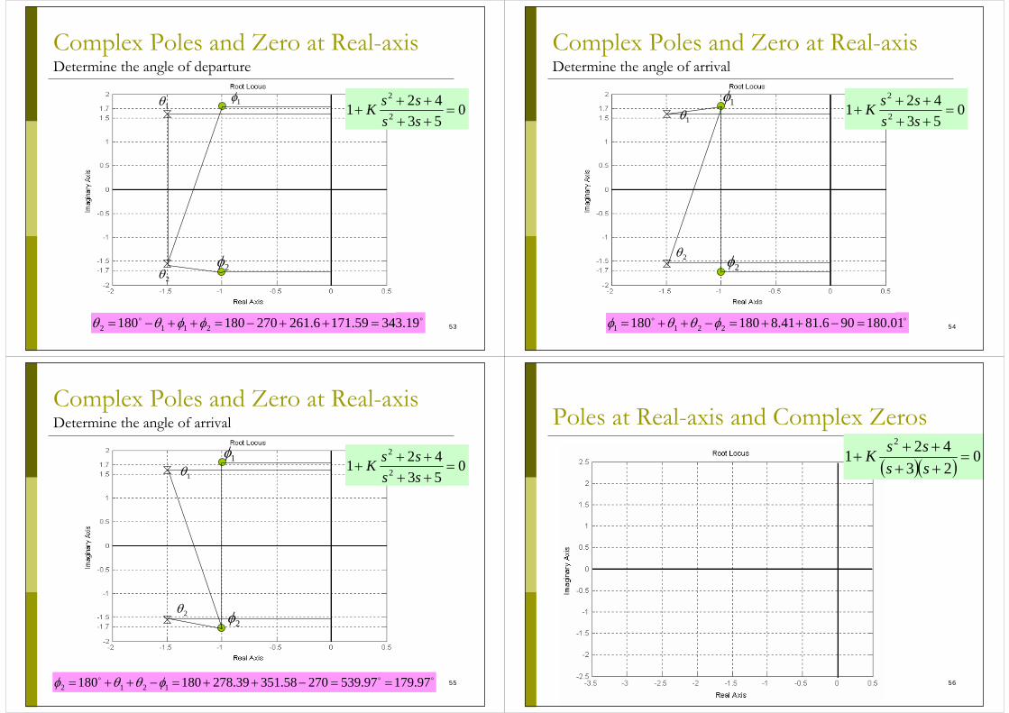
Complex Poles and Zero at Real-axis Determine the angle of departure
8.168.37639.9841.18890180180 2121 ==++−=++−= φφθθ
053421 2
2
=++++
+ssssK
2θ
1φ1θ
2φ
53
Complex Poles and Zero at Real-axis Determine the angle of departure
19.34359.1716.261270180180 2112 =++−=++−= φφθθ
053421 2
2
=++++
+ssssK
2θ
1φ1θ
2φ
54
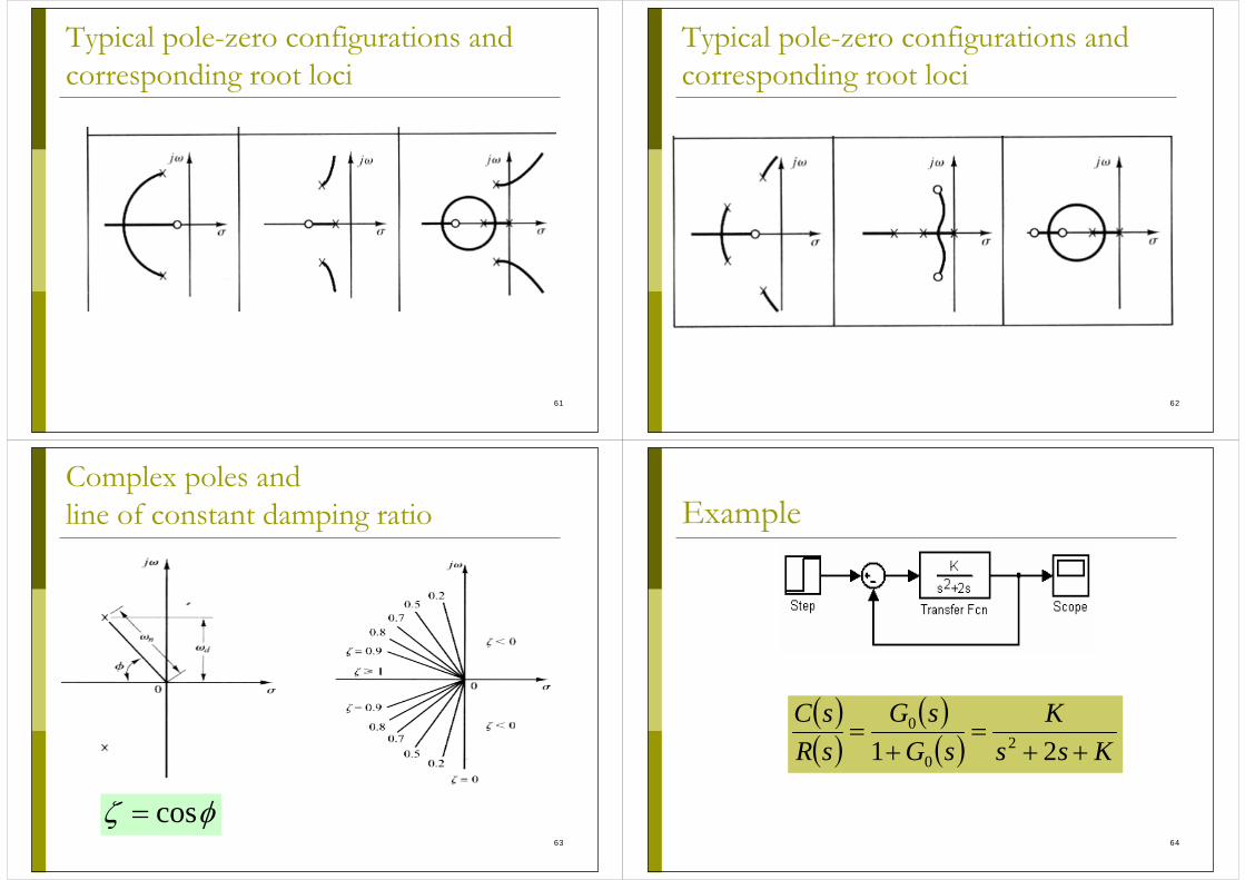
Complex Poles and Zero at Real-axis Determine the angle of arrival
01.180906.8141.8180180 2211 =−++=−++= φθθφ
053421 2
2
=++++
+ssssK
2θ
1φ1θ
2φ
55
Complex Poles and Zero at Real-axis Determine the angle of arrival
97.17997.53927058.35139.278180180 1212 ==−++=−++= φθθφ
053421 2
2
=++++
+ssssK
2θ
1φ1θ
2φ
56
Poles at Real-axis and Complex Zeros
( )( ) 023421
2
=++++
+ssssK

57
Complex Poles and Complex Zeros
( ) 053421 2
2
=++++
+sss
ssK
58
Complex Poles and Complex Zeros
( )( ) 0532
421 2
2
=+++
+++
ssssssK
59
Typical pole-zero configurations and corresponding root loci
60
Typical pole-zero configurations and corresponding root loci
61
Typical pole-zero configurations and corresponding root loci
62
Typical pole-zero configurations and corresponding root loci
63
Complex poles andline of constant damping ratio
φζ cos=64
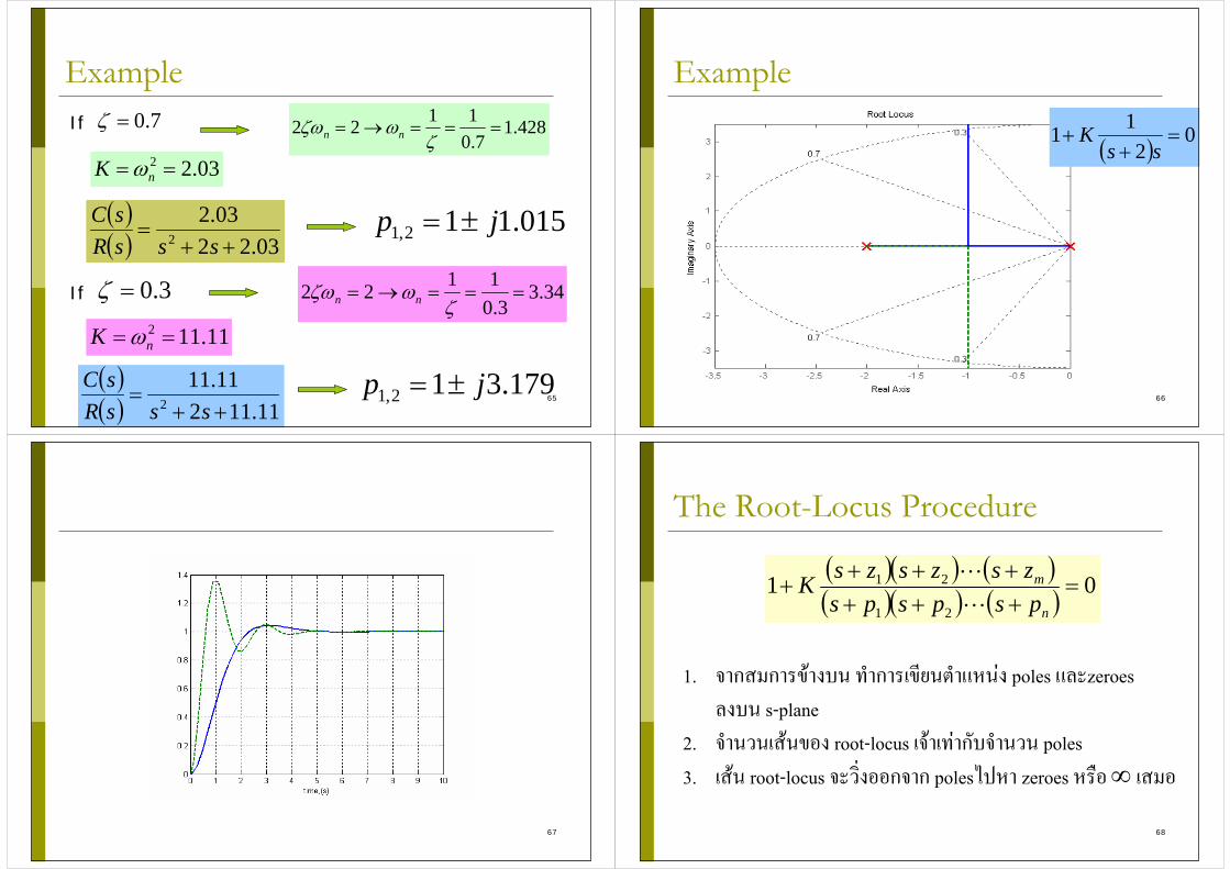
Example
( )( )
( )( ) Kss
KsG
sGsRsC
++=
+=
21 20
0
65
Example7.0=ζ 428.1
7.01122 ===→=
ζωζω nn
03.22 == nK ω
015.112,1 jp ±=
34.33.0
1122 ===→=ζ
ωζω nn
11.112 == nK ω
179.312,1 jp ±=
3.0=ζ
If
( )( ) 03.22
03.22 ++
=sssR
sC
If
( )( ) 11.112
11.112 ++
=sssR
sC66
Example
( ) 02
11 =+
+ss
K
67 68
The Root-Locus Procedure
( )( ) ( )( )( ) ( ) 01
21
21 =++++++
+n
m
pspspszszszsK
1. จากสมการขางบน ทําการเขียนตําแหนง poles และzeroes ลงบน s-plane
2. จํานวนเสนของ root-locus เจาเทากับจํานวน poles 3. เสน root-locus จะวิ่งออกจาก polesไปหา zeroes หรือ ∞ เสมอ
69
The Root-Locus Procedure
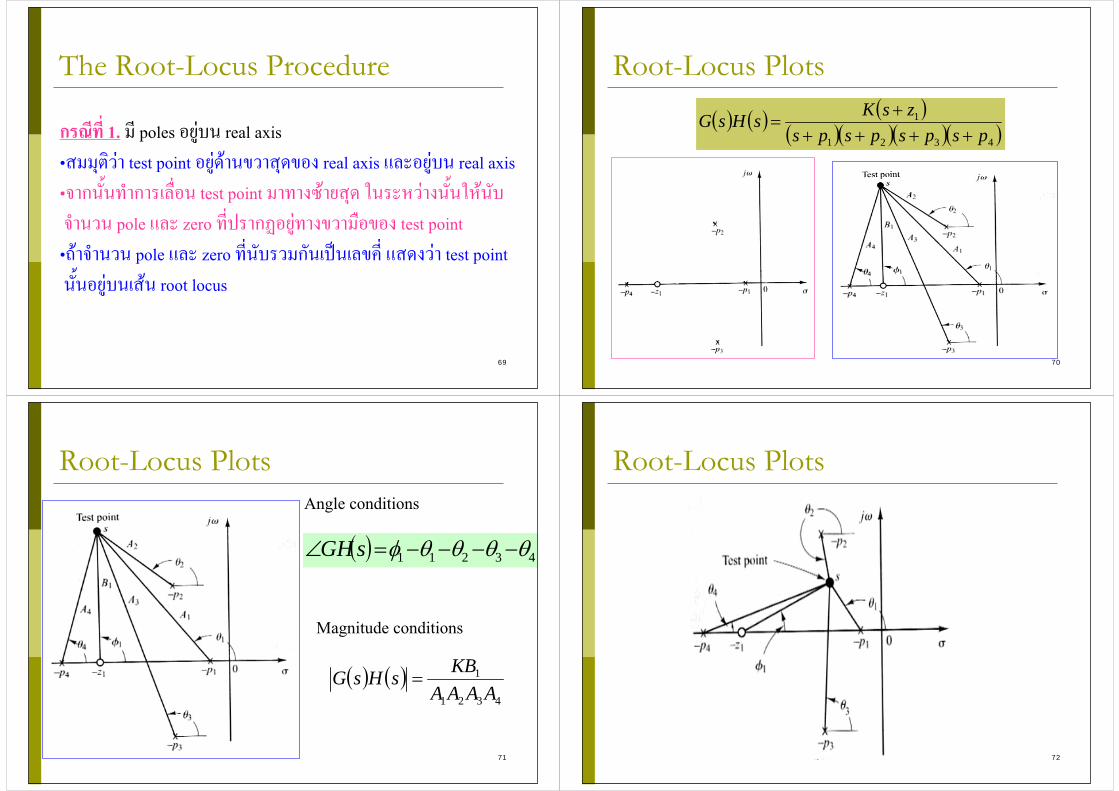
กรณทีี่ 1. มี poles อยูบน real axis •สมมุติวา test point อยูดานขวาสุดของ real axis และอยูบน real axis•จากนัน้ทําการเลื่อน test point มาทางซายสุด ในระหวางนัน้ใหนับ จํานวน pole และ zero ที่ปรากฏอยูทางขวามือของ test point•ถาจํานวน pole และ zero ที่นับรวมกันเปนเลขคี่ แสดงวา test point นั้นอยูบนเสน root locus
70
Root-Locus Plots
( ) ( ) ( )( )( )( )( )4321
1
pspspspszsKsHsG
+++++
=
71
Root-Locus Plots
( ) 43211 θθθθφ −−−−=∠ sGH
( ) ( )4321
1
AAAAKBsHsG =
Angle conditions
Magnitude conditions
72
Root-Locus Plots
73
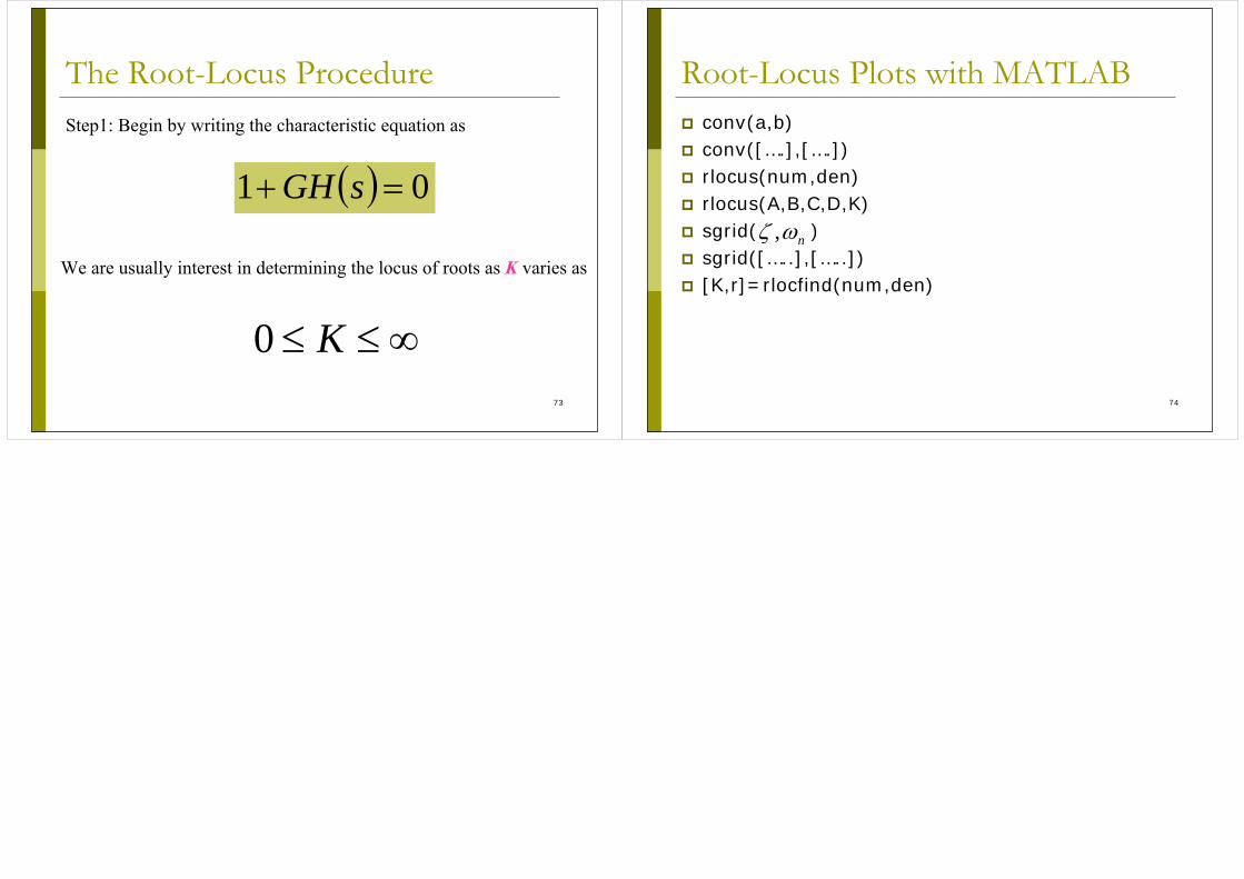
The Root-Locus ProcedureStep1: Begin by writing the characteristic equation as
( ) 01 =+ sGH
We are usually interest in determining the locus of roots as K varies as
∞≤≤ K074
Root-Locus Plots with MATLABconv(a,b)conv([….],[….])rlocus(num,den)rlocus(A,B,C,D,K)sgrid( )sgrid([…..],[…..])[K,r]=rlocfind(num,den)
nωζ ,