Estimating firm-specific long term growth rate and cost of capital

Rong Huang, Ram Natarajan and Suresh Radhakrishnan

School of Management, University of Texas at Dallas, Richardson, Texas 75083

November 2004

We are grateful to Ashiq Ali, Umit Gurun, Xu Li and participants of the seminar at the University of Texas at Dallas for their insightful comments.

Estimating firm-specific long term growth rate and cost of capital

Abstract We use the residual income valuation model to simultaneously estimate firm-specific implied long-term growth rate in abnormal earnings and cost of capital by relating earnings-to-price and book-to-market ratios in a linear fashion. This provides a simple framework to estimate the investors’ consensus beliefs with respect to long-term growth rate of abnormal earnings and the corresponding cost of capital embedded in stock price. Empirical results show that the firm-specific long-term growth rate in abnormal earnings and cost of capital estimates obtained from the model exhibit desirable properties. Specifically, both of the estimates are persistent over the years and they are related to various previously documented firm-specific factors in the predicted directions. The cost of capital estimate is also shown to be positively related to one-year-ahead and two-year-ahead returns (see Guay, Kothari and Shu (2003)). We apply the firm-specific long-term growth and cost of capital estimates to examine the value-glamour anomaly and find evidence that is consistent with the notion that the market overestimates (underestimates) the long-term growth rate of glamour (value) stocks.

1

I. Introduction

We use the residual income valuation model and derive a simple and

parsimonious method to estimate long-term growth rate in abnormal earnings and cost of

capital simultaneously. Recognizing that the analysts’ one-year ahead earnings forecasts

are available, it is shown that the earnings-to-price ratio based on the analysts’ one-year

ahead earnings forecasts is related in a linear fashion to the book-to-market ratio. The

slope coefficient on the book-to-market ratio is the long-term growth rate of abnormal

earnings, and the constant term is the effective cost of capital, i.e., the cost of capital

minus the growth rate in abnormal earnings. This relationship between earnings-to-price

and book-to-market ratio provides a simple framework to estimate the investors’

consensus beliefs with respect to long-term growth rate of abnormal earnings and the

corresponding cost of capital embedded in stock price.

The importance of obtaining a good measure of cost of capital stems from the fact

that firms and investors need to make investment decisions based on these estimates. The

financial economics literature uses the Fama-French three-factor model (see Fama and

French, 1993) to estimate the cost of capital. However, Fama and French (1997)

demonstrate the difficulties encountered in accurately estimating the cost of capital: the

three-factor cost-of-capital estimates appear to be imprecise at the firm as well as the

industry level. An alternative approach uses theoretical valuation models such as the

residual income valuation model with analysts’ earnings forecasts to obtain measures of

cost of capital by solving out for the cost of capital in the valuation expressions (see

Gebhardt, Lee and Swaminathan, 2001; Claus and Thomas, 2001; Botosan and Plumlee,

2

2002; Botosan, 1997; and Easton 2001). This is termed as the implied cost of capital

approach (see Guay, Kothari and Shu, 2003). The motivation for developing the implied

cost of capital approach is summarized by the following statement in Gebhardt, Lee and

Swaminathan (2001): “current procedures for cost-of-capital estimation advocated in

standard finance textbooks have yielded few useful guidelines for finance professionals.”

They also show how the implied cost of capital can be used for capital budgeting and

investment decisions.

The typical implied cost of capital approach uses short-term and long-term

analysts’ earnings forecasts and estimates the cost of capital that is embedded in stock

prices. While this approach can potentially improve the precision of the cost of capital

estimates as compared to an approach that uses only the past market returns (such as the

Fama-French three-factor approach), one potential problem with the analysts’ short-term

and long-term earnings forecasts stems from their sluggishness and bias. Guay, Kothari

and Shu (2003) examine this issue and show that the estimation procedures of the implied

cost of capital approaches are affected by the sluggishness of analysts’ long-term

earnings forecasts. In other words, the long-term growth rate underlying analysts’ three

to five years ahead earnings forecasts does not appear to reflect the information that is

already contained in stock prices. Thus, the analysts’ long-term earnings forecasts are

“poor” proxies for investors’ beliefs of growth, which in turn results in inefficient

estimates of cost of capital. Guay, Kothari and Shu (2003) show that sluggishness of the

3

analysts’ long-term earnings forecasts makes the association between implied cost of

capital estimates and future returns weak.1

Our approach to estimating the implied cost of capital differs from the earlier

approaches in a variety of ways. We develop a one-stage valuation model that

simultaneously estimates a firm-specific growth rate and cost of capital. Our approach

does not use analysts’ long-term earnings forecasts and thus our estimates of cost of

capital are less sensitive to biases and sluggishness of such long-term earnings proxies.

In contrast, the implied cost of capital estimates (r) is sensitive to the assumed long-term

rate of growth (g) in earlier approaches. This is because the effective cost of capital (r –

g) is what generally matters the most in the valuation expressions. Hence, whatever

value is assigned to g is correspondingly taken away from r, loosely speaking. In effect,

the implied growth rate embedded in the stock price is not considered by the earlier

approaches, while our approach takes this aspect into consideration. Another implication

of the one-stage residual income valuation model approach is that it relates two well-

known measures that are used to assess market sentiments, i.e., the earnings-to-price and

book-to-market ratios. Both these measures have been argued in the literature to be

associated with investors’ expectations of firm growth. We are not aware of any study

that formally relates these two measures and interprets the coefficients in the relationship.

The downside of our approach is that we obtain only one growth rate for

abnormal earnings, up until perpetuity. This may be a poor approximation of the linear

1 Guay Kothari and Shu (2003) evaluate the Fama-French three-factor model and various other approaches developed in the literature for estimating the implied cost of capital. They find that the Gebhardt, Lee and Swaminathan (2001) approach is associated with future returns after correcting for the sluggishness of analysts’ earnings forecasts.

4

information dynamics assumption of the residual income valuation model, especially for

start-up firms or firms experiencing extremely high growth in the short-term. However,

the extent of this problem is an empirical question which we also examine in this study.

We begin the empirical analysis by examining the validity of using the one-stage

valuation model in the cross-section. Specifically, the earnings-to-price ratio is regressed

on the book-to-market ratio annually for high, medium and low growth firms (partitioned

based on the book-to-market ratio). The estimated average growth rates are higher for the

high growth firms (low book-to-market firms) than the low growth firms (high book-to-

market firms), and correspondingly the cost of capital estimates are also higher for the

high growth firms than the low growth firms. The effective cost of capital (r – g) is lower

for the high growth firms than the low growth firms. This is consistent with the intuitive

conjecture that growth and risk are positively associated. Overall, this provides a certain

degree of validation of the one-stage residual income valuation model in the cross-

section.

Firm-specific long-term growth rate and cost of capital are estimated for each firm

using at least 24 monthly observations and up to 60 monthly observations. For about

18% of the sample at least one of the two characteristics, risk premium (which is the

difference between the cost of capital estimate and the risk-free rate) and the effective

cost of capital (which is the difference between cost of capital and growth), is negative.

This violates the assumptions underlying the theoretical residual income valuation model.

For these firm-years, we substitute the mean of the industry’s cost of capital to which the

firm belongs, where the mean is computed over all the cost of capital estimates. On

5

average, the firms with negative risk premium estimates are characterized by higher

growth in Return on Equity and Return on Assets. This is consistent with the argument

that the one-stage valuation model may not be appropriate for the firms that are in a high

growth phase.

The long-term growth estimate, on average, tracks the nominal growth rate in

GDP and the cost of capital is higher when interest rates are high, i.e., in the late 80s and

early 90s. The risk premium also follows the pattern of GDP growth, indicating that

investors demand a higher risk premium in higher growth environments. The stock

market boom in late 1990s is on average characterized by both higher growth and higher

risk premium estimates. The behavior of growth and cost of capital estimates are

persistent over time, which provides a degree of comfort about the validity of the

estimates. In other words, if the growth estimates are high in one year, but are low in

another year, any test or relationship with firm-specific factors of growth and cost of

capital could be questionable. In other words, the long-term growth and cost of capital

estimates seem to capture some fundamental features of the firm.

The validity of the firm-specific long-term growth and cost of capital estimates is

examined in two ways. First, we examine whether the estimates of growth and cost of

capital are associated with previously identified firm-specific factors related to growth

and risk; and second, we follow the Guay, Kothari and Shu (2003) methodology and

relate future returns to the cost of capital estimates. We find that the long-term earnings

growth estimate is positively and significantly related to analysts’ long-term growth in

earnings forecasts, current sales growth and current earnings growth. The cost of capital

6

estimate is positively associated with CAPM Beta and book-to-market ratio, but is

negatively associated with leverage and not associated with size. Further, the cost of

capital estimate obtained from the one-stage residual income valuation model is

positively associated with one and two-year-ahead returns. This positive association

becomes stronger after controlling for the precision of the estimates using the firm-

specific standard errors obtained from estimating the one-stage residual income valuation

model. Thus, overall the estimation methodology using the one-stage residual income

valuation model appears to capture essential elements of the long-term growth and cost of

capital embedded in stock prices.

We then demonstrate an application of the simultaneous estimation of long-term

growth in abnormal earnings and cost of capital that provides insights into the drivers of

the value-glamour anomaly. For this purpose, we form portfolios of value and glamour

firms based on the book-to-market ratio in year t; the top (bottom) thirty percent of the

book-to-market ratio firms are classified as value (glamour) firms. We then track the

growth rate in abnormal earnings and the risk premium for two years following the

portfolio formation year. The risk premium for the value firms is lower than that of the

glamour firms in all the years – contemporaneous, one-year ahead and two-years ahead.

The long-term growth rate in abnormal earnings for the glamour firms is also higher than

that of the value firms in all years. More importantly, we find that the growth rate in

abnormal earnings of glamour (value) firms decrease (increase) and the risk premium

stays almost the same. This evidence suggests that investors’ over-reaction and under-

reaction likely explains the mis-pricing of value and glamour firms. In general, the

7

simultaneous estimation of long-term growth and cost of capital embedded in stock prices

could be used to provide additional insights on anomalies that are hypothesized to be due

to “incorrect” investor beliefs about growth prospects.

Easton, Taylor, Shroff, and Sougiannis (2002) use the residual income valuation

model by using both the analysts’ short-term earnings forecasts (up to four years ahead)

and devise an iterative algorithm to estimate the cost of capital and long-term growth rate

in abnormal earnings embedded in stock prices. Specifically, they estimate a random

coefficients model where the aggregate cum-dividends earnings over the next four years

to book value of equity is expressed as a linear function of price-to-book ratio. In their

formulation the constant term in the valuation expression is (g) and the slope coefficient

is (r – g). In contrast, the slope coefficient on the book-to-market ratio in our valuation

expression is (g) and the constant term is the effective cost of capital, (r – g). Easton,

Taylor, Shroff, and Sougiannis (2002) use an iterative algorithm to obtain the estimates

because the aggregate cum-dividends earnings contain the cost of capital. The

methodology proposed in this paper has the advantage that simple OLS regression can be

used to operationalize the model and estimate the long-term growth in abnormal earnings

and cost of capital simultaneously. Furthermore, operationalizing Easton, Taylor, Shroff,

and Sougiannis’s (2002) algorithm for a time-series may be difficult. While the portfolio

approach of estimating cost of capital and growth rates using the random coefficient

model has the advantage of the assumption that the cost of capital for each firm in the

portfolio is a draw from a distribution, and there are no time-invariant assumptions

embedded in the estimation; our estimation procedure has the assumption that the firm’s

8

cost of capital and growth rates are time-invariant during the estimation period.

However, this time invariance assumption has to be made for any estimation procedure

that uses time-series data.

The paper is organized as follows: Section II develops the residual income

valuation model and the valuation expression for the estimation, introduces the data and

sample used for the estimation procedure and validates the valuation expression by

examining the behavior of the estimates for portfolio of firms cross-sectionally; Section

III provides the firm-specific estimates of growth and cost of capital and examines the

persistence behavior of the estimates; Section IV tests the veracity of the estimates;

Section V provides a potential application of the methodology and Section VI contains

some concluding remarks.

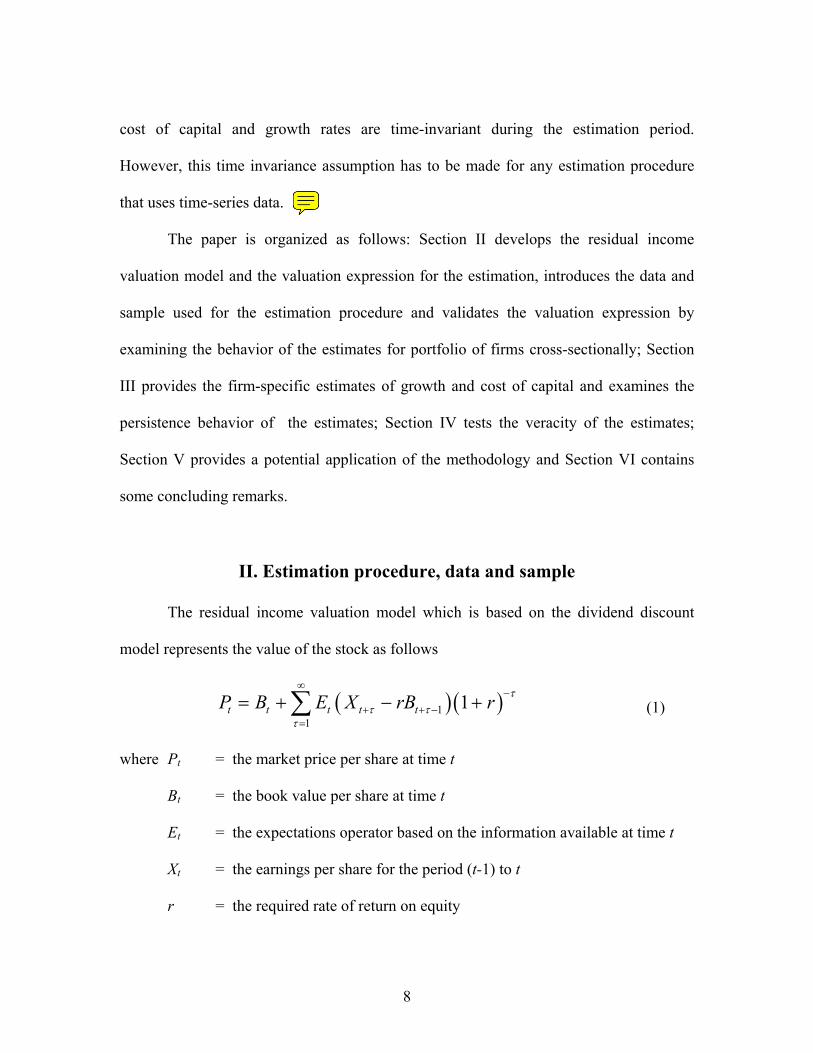
II. Estimation procedure, data and sample

The residual income valuation model which is based on the dividend discount

model represents the value of the stock as follows

( ) ( )11

1t t t t tP B E X rB r ττ τ

τ

∞−

+ + −=

= + − +∑ (1)

where Pt = the market price per share at time t

Bt = the book value per share at time t

Et = the expectations operator based on the information available at time t

Xt = the earnings per share for the period (t-1) to t

r = the required rate of return on equity

9

The value of the stock is represented as the value of the assets-in-place plus the

present value of future abnormal earnings. The abnormal earnings ( 1atX + ) for any time

period t to (t+1) is given by

1 1at t tX X rB+ += − (2)

We assume that the abnormal earnings grow at a perpetual constant rate (g), and

hence

11 (1 )a a

t t tE X X g ττ

−+ + = + for 1τ > . (3)

Equation (3) is specified for 1τ > , recognizing that in general the one period

ahead earnings forecast is available to the investors. Of course, in general, the two period

and three period ahead forecasts along with a long term growth rate that indicates the

growth rate up to five years ahead are also provided by some analysts. We restrict our

attention to one year ahead forecasts because the forecast errors of the two, three and

higher horizon forecasts are much larger. This helps in expressing the residual income

valuation formula in equation (1) in a simple and parsimoniously estimable form; as will

become evident shortly.

Using equation (3) in equation (1) we have

10

( )

( )

( )

( )

2 3

1

1

1

1

(1 ) (1 ) (1 )1 ...

(1 ) (1 ) (1 ) (1 )

(1 )(1 ) ( )

( )

( )

t tt t

t tt

t tt

t t

X rB g g gP B

r r r r

X rB rB

r r g

X rBB

r g

X gBr g

+

+

+

+

− + + += + + + + +

+ + + +

− += +

+ −

−= +

−

−=

−

Rearranging the above valuation representation we have

1 ( ) t t

t t

X Br g gP P+ = − + . (4)

Equation (4) represents the relationship between the book value of equity, one-

year-ahead earnings and stock price for any given firm j at any point in time t. Thus, from

equation (4) we can write the following linear relation for each firm j

( 1)0 1 j t jt

j j jtjt jt

X Be

P Pγ γ+ = + + (5)

where ejt is the error term, jjj gr −=0γ and jj g=1γ . Notice that equation (4) does not

have an error term, whereas equation (5) does. The growth of future abnormal earnings

in equation (3) can be construed as a draw from a distribution in each time period t with a

mean jtg and variance 2gjσ . That is, the growth in abnormal earnings, jtg , is random and

is based on the information available on the firm and the environment in each time period

t. We can also consider the cost of capital jtr in a similar fashion, especially because it is

11

made up of the risk free rate and a risk premium and the risk free rate is stochastic. The

error term arises because of the random components of jtg and jtr 2.

The representation in equation (5) relates the earnings-to-price (EP) ratio to the

book-to-market (BM) ratio. The estimate 1jγ captures the covariance of EP and BM ratios.

Specifically, when the covariance between EP and BM ratios is positive and high it will

imply high growth prospects; while, when the covariance is low the growth prospects for

the firm are limited or small. We estimate equation (5) cross-sectionally to validate the

basic precepts of the model and then proceed to estimate the growth and cost of capital

for each individual firm using equation (5). As in Easton, Taylor, Shroff, and Sougiannis

(2002) the main benefit of using this approach is that estimates for both the firm-specific

cost of capital and the growth rates are obtained simultaneously.

The data and sample

We obtain book value of equity (data item # 60) from the 2002 Compustat Annual

Industrial Database, the stock price and the number of common shares outstanding at the

end of each month from CRSP, and the one-year ahead analysts’ mean consensus

earnings forecasts from the summary I/B/E/S file. Earnings forecasts and book value of

equity are matched such that at each month end, EP and BM contain the most recent

information available to the market. Firms with negative EPS forecast are deleted

because these are not consistent with the assumptions embedded in the theoretical model.

Firms with sales less than 10 million, book value less than 5 million, fiscal-year closing

price less than $1 and less than two analysts are also deleted so as to restrict attention to 2 Specifically jte = ( jtr - jtg )-( j jr g− ) + ( jtg jg− ) jt jtB P .

12

sufficiently large firms. The final sample contains 34,204 firm-year observations,

spanning from 1985 to 2001. The number of firms in the sample ranges from 1,330 in

1985 to 2,895 in 1998.

Validating equation (5) cross-sectionally

Before proceeding with the firm-specific estimation of the growth and cost of

capital, we examine whether the model specified in equation (5) is validated in the cross-

section. For this purpose, we estimate equation (5) annually for three partitions of the

sample based on the book-to-market ratio. We use NYSE/AMEX book-to-market break

points to determine the book-to-market group the firm belongs to. That is, each year firms

with book-to-market ratio in the top (bottom) thirty percent of NYSE/AMEX sample are

assigned to the high (low) book-to-market ratio group; and the remaining forty percent

are assigned to the medium book-to-market group. The high (low) book-to-market ratio

group is considered to be value (glamour) stocks. In general, prior studies have shown

that glamour (value) stocks yield negative (positive) risk-adjusted abnormal returns over

two to three years. Fama and French (1992, 1993), Chan and Chen (1991) show evidence

consistent with value stocks yielding positive abnormal returns in the future because of

an additional risk premium for financial distress; that is, the high book-to-market group

have low earnings prospects and are in financial distress and consequently, the required

rate of return (cost of capital) is also higher. This argument centers around the fact that

traditional risk measures (such as the CAPM beta) do not capture these risk factors.

Based on these arguments we expect to find the cost of capital to be higher for the high

book-to-market group than the low book-to-market group. On the other hand, book-to-

13

market represents the intangible intensity of the firm and consequently, the book-to-

market ratio is a proxy for growth possibilities (see Lakonishok, Shleifer and Vishny

(1994) and Piotroski (2000)). For instance, high research and development activity firms

are also found to be low book-to-market firms (see Lev and Sougiannis (1996)). Thus,

the market perceptions of growth opportunities for the low book-to-market firms will be

higher than the growth opportunities of the high book-to-market firms. Based on this we

expect the growth estimate for the low book-to-market firms to be higher than that of the

high book-to-market firms.

Table 1 shows the descriptive statistics of some key variables: market value of

equity, book value of equity, total sales, total assets, earnings-to-price ratio, book-to-

market ratio, debt-to-equity ratio and number of analyst following. The mean (median)

market value of equity, book value of equity, sales and total assets are $2,152 (302), $874

(156), $1,999 (324) and $4,492 (399) million, respectively showing that there are few

large sized firms and a large number of small sized firms. This also shows that the

sample contains a wide variation of firm size, measured using either market capitalization

measures or accounting based measures. The mean (median) earnings-to-price ratio is 7%

(7%) which corresponds with a price-to-earnings ratio of about 14. In general, the

sample contains both value and glamour firms, i.e., a wide variation in the price-to-

earnings ratio which has traditionally been used as a measure of the market’s growth

expectation. The mean (median) book-to-market ratio is 1.65 (0.53) which corresponds

with a market-to-book ratio of about 0.6 (2) on average. In general, the sample contains a

wide variation of firms in terms of intangible intensity as measured by the market-to-

14

book ratios. The median debt to equity ratio is 0.31 and there are 11% of firms with no

debt, i.e., having a debt to equity ratio of zero. The mean (median) number of analysts

following a firm is 8 (5), which show that a large number of analysts follow a few firms

and vice versa. Overall, the sample contains a wide variation in firm-size, intangible

intensity and analyst following.

Table 2 provides the results of estimating equation (5) each year for the low,

medium and high book-to-market groups. Panel A of Table 2 provides the distribution of

the growth estimates obtained by estimating equation (5) for each of the 17 years. The

growth, on average is about 6.5% for the low book-to-market group and zero percent for

the high book-to market group. This suggests that on average the investors believe that

the low book-to-market firms have better investment opportunity sets and consequently

better growth opportunities. The growth estimates ranges from a minimum of 3.3% in

year 2001 to a maximum of 9.5% in year 1999 for the low book-to-market group; while

the growth estimate for the high book-to-market group is zero for all the 17 years. This is

consistent with our conjecture that investors have no growth expectations for the

financially distressed firms (i.e., the high book-to-market group) and that the investors

have positive growth expectations for the intangible intensive firms (i.e., low book-to-

market group).

Panel B of Table 2 provides the distribution of the cost of capital estimates

obtained by estimating equation (5) annually for each of the 17 years. The cost of capital

estimate for the low book-to-market group on average is about 10.3%; while that for the

high book-to-market group is about 8.3%, representing an average difference of about

15

2.0%. The cost of capital estimate ranges from a minimum of 6.6% in year 2001 to a

maximum of 12.8% in year 1988 for the low book-to-market group; while the minimum

costs of capital estimate for the high book-to-market group is 6.3% in year 1997 and the

maximum is 10.9% in year 1990. The cost of capital estimates for the low book-to-

market group is greater than that for the high book-to-market group in 16 out of the 17

years. Overall, the annual distribution of the cost of capital estimates suggests that the

financial distress argument posited in earlier studies, i.e., the investors demand a higher

rate of return for the high book-to-market firms due to the risk of financial distress is not

directly supported by the estimates.

Panel C of Table 2 shows the effective cost of capital, i.e., (r – g) cost of capital

that is adjusted for growth expectations. The effective cost of capital required by the

investors after adjusting for growth opportunities, i.e., (r – g) is higher for the high book-

to-market ratio firms The effective cost of capital estimate on average is 8.3% for the

high market-to-book firms as against 3.8% for the low market-to-book firms. Notice that

[1/(r – g)] is the valuation multiplier on the present value of future abnormal earnings and

the (r – g) estimates correspond to the valuation multipliers of about 26 (12) for the low

(high) book-to-market group. The distribution of the annual effective cost of capital

estimate ranges from a minimum of 2.7% and a maximum of 4.5% for the low book-to-

market group; while the distribution of the annual effective cost of capital estimate ranges

from a minimum of 6.3% and maximum of 10.9% for the high book-to-market group.

The effective cost of capital for the low book-to-market group is lower than the effective

cost of capital estimate for the high book-to-market group for each of the 17 years. This

16

lends a certain degree of support to the intuition that the effective cost of capital is higher

for the financially distressed firms as argued in earlier studies. Overall, the evidence

supports the basic precept of a positive relationship between growth and cost of capital.

Specifically, a higher growth is deemed to be risky and hence the maintained assumption

is that investors will demand a higher rate of return for the higher growth companies (see

Damodaran, 1997). For instance, start-up firms for which venture capitalists provide

seed capital, very high rates of return (discount rates) are used because even though such

companies have the potential for high growth they are perceived to be high risk. The

evidence supports the notion underlying this intuition. However, the evidence shows that

the effective cost of capital, i.e., the cost of capital adjusted for the growth expectations is

lower for firms with high growth expectations. The estimation of equation (5) in the

cross-section provides a certain degree of support for the representation of the valuation

model.

We move to estimating firm-specific growth and cost of capital estimates.

III. Firm-specific estimation of growth and cost of capital

The valuation representation in equation (5) is used to obtain firm-specific growth

and cost of capital estimates. Specifically, equation (5) is estimated separately for each

firm, using at least 24 months time-series observations up to a maximum of 60 months

time-series observations on a rolling basis. In other words, to obtain firm-specific

estimates of equation (5) for 1998, we use the monthly analysts’ consensus earnings

forecasts, book value of equity for the closest preceding fiscal year and monthly stock

17

prices for 1994, 1995, 1996, 1997 and 1998.3 The sample contains 28,601 firm-year

observations from 1985 to 2001. The number of firms range from 1,104 in 1985 to 2,494

in 2000.

Firm characteristics where the risk premium or effective cost of capital is negative

Out of the 28,601 firm-years in the sample with available time-series data, at least

one of the two characteristics, risk premium (which is the difference between the cost of

capital estimate and the risk-free rate) and the effective cost of capital (which is the

difference between cost of capital and growth), is negative for 5,229 firm-years, which is

about 18% of the sample. Theoretically, both the risk premium and the effective cost of

capital have to be positive. Thus, the firm-specific estimation of equation (5) yields

theoretically inconsistent estimates for about 18% of the firm-years.

Panel A of Table 3 provides some characteristics of firms for which we obtain

negative effective cost of capital estimates. One possible explanation for such negative

estimates is that for some firms growth in the short run is extremely high. Panel A

shows that the mean growth in operating income, ROA and ROE are much higher for

firms with negative estimates for effective cost of capital than for firms with positive

effective cost of capital estimates. For example, Walmart had growth estimates above

30% from 1986 to 1989; and Johnson and Johnson had growth estimates of about 40%

from 1993 to 1995. In unreported analysis, we find that firms with negative risk premium

estimates are mostly financially distressed, such as LTV and U.S. Steel.

3 We use the book value of equity obtained from the quarterly Compustat and obtain very similar results.

18

The descriptive statistics of the firm-specific estimates

Panel B (Panel C and Panel D) of Table 3 provides the yearly mean, median and

standard deviation of firm-specific estimates of the growth (g), (cost of capital (r), risk

premium (r – rf) and effective cost of capital (r - g)), where the risk free rate, rf is the ten

year treasury bill rate. For the 18% of the firm-years with either negative risk premium

or negative effective cost of capital the average industry cost of capital for the same year

is substituted. Thus, for such firms the effective cost of capital and risk premium is

recalculated after substituting for the firm’s cost of capital with the industry’s cost of

capital. This adjustment procedure results in positive values for risk premium and

effective cost of capital for 2,769 out of the 5,229 firm-years that have either negative

risk premium or negative effective cost of capital.

The median growth estimate during the period 1986 to 1989 is around 8.5% and

then drops to around 7% during 1990 through 1996 and then increases to about 7.5% up

until 2000 during the boom years (see Panel B). The median cost of capital is about

12.5% to 13.0% during 1986 through 1990 and then drops to about 11.0% in the 1990s

(see Panel C). The median risk premium estimates hold steady at around 5% for the 17

years (see Panel C). The risk premium moves in consonance with the growth estimates,

which suggests that investors perceive higher growth as more risky and demand a higher

risk premium. The median effective cost of capital, i.e., (r – g) is around 3.7% during

1987 through 1992 which corresponds with a valuation multiplier on abnormal earnings

of about 27; and during the boom years in the late 1990s the median effective cost of

19

capital is around 2.5% which corresponds with a valuation multiplier on abnormal

earnings of about 40 (see Panel D).

The average growth is about 8.1%, average risk premium across all the years is

5.9%, and the effective cost of capital is about 3.9% indicating that the average valuation

multiplier is about 25 on the abnormal earnings. The annual average growth estimates

tracks the growth in nominal GDP, i.e., the growth estimates is the lowest in the

recessionary years (early 90s) and highest in the boom years (late 90s). The average risk

premium in 1998, 1999 and 2000 was 6.8%, 6.7% and 6.1%, respectively as against 5.8%,

5.9% and 6.0% in 1995, 1996 and 1997, respectively. This suggests that even during the

dotcom bubble the investors on average demanded a higher required rate of return on the

potentially high growth stocks (a full percent higher than the period just prior to the

dotcom boom). It is interesting to note that after the dotcom bubble, i.e., in 2001 the risk

premium continued to be higher (6.7%) potentially due to the market melt down and the

plethora of scandals and break down of governance mechanisms.

Panel E of Table 3 provides the mean and median estimates of cost of capital and

risk premium in our sample based on the Ohlson-Juettner model (see Gode and

Mohanram, 2003). We use the Ohlson-Juettner model based estimates for comparison

purposes in the validity tests for the estimates based on equation (5). This procedure of

computing cost of capital is used in our further analysis, mainly to show that our sample

is similar to that of Gode and Mohanram (2003). In other words, by using the Gode and

Mohanram (2003) procedure to estimate cost of capital we do not use it as a benchmark

for the “best” measure of cost of capital. We choose the Gode and Mohanram (2003)

20

procedure mainly because it is simple to compute. The average median risk-premium

estimate for our sample estimated using the Ohlson-Juettner model is 5.9% which is quite

comparable to the risk premium reported by Gode and Mohanram (2003).

Persistence of the growth and risk premium estimates

The growth measures and the risk premium measures should exhibit a certain

degree of persistence. We expect a certain degree of persistence with the growth measure

because the growth measure estimated through equation (5) is a long term growth

measure. If the growth exhibits no consistent pattern, in the sense that firms with high

growth in year t become low growth firms in future years or do not show any consistent

pattern then either the investors’ perceptions of long-term growth are extremely fickle or

the estimation procedure of equation (5) is not appropriate. In a similar vein, the risk

premium is a long-term firm characteristic, theoretically speaking, and hence, we would

expect a certain degree of persistence in the risk premium estimates.

Table 4, Panel A provides the persistence of the firm-specific growth estimates.

For this purpose, in each year t we classify firms as being high, medium and low growth

and track the growth profiles for these firms in years (t+1) and (t+2). Specifically, in each

year we classify the top (bottom) 30% of firms as the high (low) growth firms with the

remaining 40% being classified as the medium growth firms. For each group of firms in

year t, we compute the average growth one and two years after portfolio formation. To

maintain both surviving and non-surviving firms in our sample and thus mitigate a

sample selection bias, we adopt the following approach. We calculate the Altman’s

(1968) Z-score as a proxy for the general financial health of the company in year t. We

21

rank the firms according to their Z-scores in their industry group and assign each firm

into the high, medium or low Z-score group. For each industry-Z score grouping, we

compute the mean growth and risk premium for all the surviving firms. If a firm belongs

to a companion industry-financial health portfolio high in year t, and does not survive in

year (t+1), we substitute the mean of the companion industry-financial health portfolio

for that firm in year (t+1).

The low growth firms in year t, have current year, one-year ahead and two-years

ahead median growths of 0%, 0.5% and 1.8%, respectively showing an increase of about

1.8% over the years. Similarly, the medium growth firms in year t, have current year,

one-year ahead and two-years ahead median growths of 7.2%, 7.3% and 7.4%,

respectively; thus showing a slight increase of about 0.2% over the three years. The high

growth firms in year t, have current year, one-year ahead and two-years ahead median

growths of 15.9%, 14.5% and 12.7%, respectively; thus showing a considerable decrease

of about 3% over the three years; which indicates a certain degree of reversal to the

average. However, on average the low, medium and high growth firms continue to be as

such even after two years. More specifically, even with the considerable drop of 3% in

growth rate estimates of the high growth firms, the medium growth firms continue to

have a growth rate that is 5.3% lower than that of the high growth firms (a difference

higher than the drop in growth estimates for high growth firms). Similarly, the low

growth firms have a difference of about 6% when compared with the medium growth

22

firms in all years. Thus, our estimation procedure appears to capture some fundamental

elements of growth characteristic of firms.4

Panel B of Table 4 provides the persistence profiles of the risk premium estimates.

The low risk premium firms in year t, have current year, one-year ahead and two-years

ahead median growths of 2.5%, 3.4% and 4.5%, respectively, showing an increase of

about 2% over the three years. Similarly, the medium risk premium firms in year t, have

current year, one-year ahead, two-years ahead and three-years ahead median risk

premiums of 6.1%, 6.3% and 6.5%, respectively; increasing slightly by 0.4% over the

three years. The high risk premium firms in year t, have current year, one-year ahead and

two-years ahead median risk premiums of 10.9%, 10.3% and 9.5%, respectively; thus

showing a decrease of about 1.4% over the three years; which indicates a certain degree

of reversal to the average. However, on average the low, medium and high risk premium

firms continue to be as such even after three years. The trend of persistence of the risk

premium estimates follows the pattern of the persistence of growth. That is as growth

estimates decrease over time the risk premium also decreases.

Panel C of Table 4 shows the persistence pattern of effective cost of capital.

Similarly, firms with low effective cost of capital continue to have low estimates over the

next two years, and firms with high effective cost of capital continue to have high

estimates for the next two years.

Panels D and E of Table 4 provides the persistence of the standard errors of the

growth and cost of capital estimates. This is one important and interesting feature of the

4 The rolling window that is used in estimating equation (5) could induce some level of persistence due the overlap in the years. We used a three year rolling window and obtained qualitatively similar results.

23

firm-specific estimation of equation (5). In addition to the estimates of growth and cost

of capital we also get the estimate of the precision of the growth and cost of capital

estimates. We report the average standard errors of the growth and cost of capital

estimates in Panels D and E respectively. The standard errors of low and medium

standard error groups for both growth and cost of capital increases slightly across years,

showing that the precision of growth and cost of capital estimates for these two groups

declines slightly. The standard error of the high standard error group exhibits a sharp

decline showing that the precision improves over time as the investors learn more about

the fundamentals of the firm.

To summarize, the results in Table 4 suggest that investors’ perceptions of growth

and risk are not fickle and exhibit a certain degree of persistence that would be

characterized by some fundamental traits of firms. We now turn to testing the validity of

the estimates.

IV. Tests of the estimates of growth and cost of capital

In this section we test the estimates of cost of capital and growth by examining

their association with some intuitive determinants; and then examine whether the cost of

capital estimates are related to the future returns.

Risk premium and firm characteristics

Following Gebhardt, Lee and Swaminathan. (2001) and Gode and Mohanram

(2003) we examine the cross-sectional relation between the firm-specific risk premium

estimate and various factors that have been documented to be associated with cost of

24

capital. The factors that Gebhardt, Lee and Swaminathan (2001) consider are Beta

obtained from the CAPM model, size, book-to-market, leverage, unsystematic risk,

dispersion of analysts’ earnings forecasts, long term growth and the average industry

implied risk premium. Gebhart, Lee and Swaminathan (2001) include these variables by

examining the univariate correlations of the variables with their estimate of the risk

premium. They include dispersion of analysts’ forecasts and the analysts’ long-term

earnings growth rate because they use the growth estimates directly in computing the

implied cost of capital. As against this, we use only the analysts’ one-year ahead

earnings forecasts. Thus, we do not control for these analyst based measures in our test

of the determinants of risk premium. Specifically, we consider the following firm

characteristics: CAPM Beta, log of market value of equity, log of book-to-market ratio

and log of debt-to-market value of equity ratio; where CAPM Beta is estimated using at

least 24 month up to 60 months data immediately preceding the test year; the market

value of equity is price times shares outstanding at the end of June in the test year. Book-

to-market ratio is calculated as the book value of the preceding fiscal year divided by the

market value of equity at the end of December of last calendar year (Fama and French

(1993)). Debt-to-market value of equity ratio is calculated using the long-term debt of

the preceding fiscal year divided by the market value of equity at the end of December of

last calendar year.

The results of examining the association between firm characteristics and risk

premium are provided in Table 5. We estimate the model annually and Table 5 reports

the mean coefficient estimates and the t-statistics are based on the time-series estimates

25

obtained for the annual estimation (see Fama and MacBeth, 1973). Risk premium is

positively related to CAPM Beta with an average coefficient of 0.22. The coefficient on

CAPM Beta is positive for 13 out of the 17 years; and is statistically significant for 4 out

of the 17 years. The log of market value of equity is not associated with risk premium,

when all the years are considered together. However, for 11 out of the 17 years the

estimate is negative as expected and is statistically significant for 3 years. The log of

book-to-market ratio is positively associated with risk premium in 15 out of the 17 years,

and is significant in 3 years. The association of risk premium with CAPM Beta, firm-size

and book-to-market are consistent with the findings of Gebhart, Lee and Swaminathan

(2001) and Gode and Mohanram (2003). In general, our finding of negative association

between leverage (log of debt to book value of equity) for 14 out of the 17 years, in

which it is significant for two years, is inconsistent with earlier findings. Specifically, a

high leverage is expected to be positively associated with risk (see Bhandari, 1988).

However, higher debt levels could be negatively associated with risk if lenders are

generally reluctant to extend credit to firms which are in the high-technology industry,

which exhibits high growth. Note that high growth is positively associated with cost of

capital, and hence risk premium (see Table 2). In our estimation procedure, which allows

for the endogenous estimation of long-term growth, this countervailing factor could lead

to the insignificant association between risk premium and debt to equity ratio.

Panel B of Table 5 provides the results of the determinants of risk premium when

risk premium is measured by the Ohlson-Juettner model following Gode and Mohanram

(2003) procedure. Consistent with our findings CAPM Beta and book-to-market are

26

positively associated with risk premium measured by the Gode and Mohanram (2003)

procedure. Firm-size is strongly negatively associated and leverage is positively

associated with risk premium measured by the Gode and Mohanram (2003) procedure.

This suggests that the leverage and firm-size associations with our estimates of risk

premium that we find (see Panel A of Table 5) are not due to sample characteristics, but

more due to the difference in estimation procedure. The main difference between Gode

and Mohanram (2003) and our estimation procedure is that they allow for a two-stage

growth model as against our single-stage growth model. In effect, we do not use the

analysts two-year ahead and long-term growth forecasts in estimating the risk premium.

We will examine the performance of our estimates vis a vis the Gode and Mohanram

(2003) estimates using the realized returns shortly.

Association of growth estimate with growth characteristics of firms

We examine the cross-sectional relation between firm-specific estimates of the

investors perceived growth in future abnormal earnings as estimated through equation (5)

and various growth measures. Specifically, the growth measures that we consider are the

analysts’ long-term earnings growth forecasts, the past sales growth and past earnings

growth. The analysts’ long-term earnings growth forecast is obtained from I/B/E/S. The

sales growth is computed as the difference of sales (Compustat #12) between year t and

year t-1 divide by the sales in year t-1. Similarly, the earnings growth is computed

relative to the prior year using earnings before extraordinary items (Compustat #18).

Note that our growth estimate, theoretically speaking, is the growth estimate of abnormal

earnings.

27

The results of examining the determinants of our growth estimates are reported in

Panel C of Table 5. The analysts’ long-term earnings growth forecast, the past earnings

growth and the past sales growth are all positively associated with the growth in

abnormal earnings estimate that we obtain by estimating equation (5).

We next turn to performing another series of tests that seek to further validate our

cost of capital measure.

Future returns and cost of capital estimates

The firm-specific estimates of cost of capital are empirically validated using the

methodology in Guay, Kothari and Shu (2003). Guay, Kothari and Shu’s (2003)

methodology is based on the standard methodology in the financial economics literature,

which uses the time-series average of the estimated coefficients from Fama-MacBeth

cross-sectional regressions of returns on betas or the estimated cost of capital (see Fama

and MacBeth, 1973, Campbell, Lo, and MacKinlay, 1997). If the time-series average

coefficient is significantly positive then it lends some degree of support to the joint test of

the validity of the measure and market efficiency.5 Specifically, we compare the ability

of our cost of capital estimate and the Ohlson-Juettner estimate using the Gode and

Mohanram (2003) procedure to explain cross-sectional variation in realized future

returns. Fama-MacBeth type regressions are estimated using Ordinary Least Squares

(OLS). As pointed out by Guay, Kothari and Shu (2003) we control for the sluggishness

of analyst forecasts by including past returns as a control variable. We also examine

whether our estimates of cost of capital explains the cross-sectional variation in realized

5 In its strong form the time-series average of the coefficients should be one.

28

future returns by using the Weighted Least Square (WLS) estimation procedure annually.

The weights for the WLS procedure are based on the inverse of the standard error of the

cost of capital estimate. Notice that the standard error of the cost of capital estimate that

we obtain enables us to weight the cost of capital estimates.

Panel A of Table 6 provides the results of Fama-MacBeth regressions of one- and

two-year ahead returns on the estimate of cost of capital from equation (5) and the

Ohlson-Juettner model and the risk premium. We find that the average coefficient on

cost of capital estimates from the Ohlson-Juettner model is -0.36 with a t-statistic of -1.47,

i.e., on average the cost of capital estimate is negatively associated with future returns.

Consistent with Guay, Kothari and Shu (2003), the cost of capital estimate and the risk

premium estimate obtained from the Ohlson-Juettner model is negatively correlated with

future returns for 11 out of the 17 years, and the negative coefficient is statistically

significant for 9 out of the 17 years. In contrast, our estimate of cost of capital is

positively associated with one-year-ahead returns for 13 out of the 17 years, and the

positive coefficient is statistically significant for 9 out of the 17 years. The average of the

annual coefficient is 0.23 for one-year-ahead returns with a t-statistic of 1.56. Thus, our

estimate of cost of capital has the desired feature that it is positively associated with

future returns, albeit weakly in the statistical sense.

Panel A of Table 6 also provides the results of Fama-MacBeth regression of one-

year ahead returns on the estimate of cost of capital from equation (5) and the Ohlson-

Juettner model along with a control for past returns. We find that the average coefficient

on the cost of capital estimates from the Ohlson-Juettner model continues to be -0.36

29

with a t-statistic of -1.47, i.e., Gode and Mohanram’s (2003) estimate of cost of capital is

negatively associated with future returns. As against this, the average coefficient on our

cost of capital estimates drops to 0.15 from 0.23 and the t-statistic drops from 1.56 to

1.06. Moreover, with the control on past returns the coefficient on our estimate of cost of

capital is positive for 11 out of the 17 years and is significant for 7 out of the 17 years.

As Guay, Kothari and Shu (2003) argue stock prices in general will adjust to

information more quickly than analysts’ forecasts leading to any estimate of cost of

capital based on analysts’ information to be negatively correlated with recent stock price

performance. If recent stock prices have been high, and if analysts’ forecasts of future

earnings are too low due to sluggish updates of the information that has been recently

impounded in stock price, the estimate of the intercept in our model will be biased

downwards, leading to a lower estimate of cost of capital. This potential bias is controlled

for using the past returns. If there is no such bias we would expect the estimates of cost

of capital to continue to be positively associated with future returns. Based on these

arguments the results suggest that the sluggishness of the analysts’ estimates argued in

Guay, Kothari and Shu (2003) appears to make our cost of capital estimate less reliable.

The sluggishness of analysts’ forecasts is well-documented in the literature that

examines analysts’ forecast bias. One reason for analysts’ bias could be that analysts’

earnings forecasts are optimistic. (see Stickel, 1990, Abarbanell, 1991, Brown, et al.,

1985, Brown, 1997, Lim, 2001, and Gu and Wu, 2003 for discussions of analyst forecast

bias). If analysts’ earnings forecasts are optimistic, then the intercept estimate from

equation (5) is likely to be biased upwards, i.e., our estimate of cost of capital is biased

30

upwards. Abarbanell and Lehavey, (2003) identify two asymmetries in forecast errors

and attribute the findings of analysts’ bias to these asymmetries.

However, as Guay, Kothari and Shu (2003) find, if analysts’ are sluggish in

incorporating the information contained in stock prices into their earnings forecasts, that

is there is a delay in the analysts’ updating their forecasts, then the standard error of our

cost of capital estimates would be higher. The standard error of our cost of capital

estimates can also be high if the stock prices themselves are not informative and the

accounting-based information itself is not informative. For these reasons we weight each

firm-specific cost of capital estimate by the inverse of the standard error of the cost of the

capital estimate obtained when estimating equation (5).

Panel B of Table 6 provides the results of Fama-MacBeth regression of one- and

two-year ahead returns with our estimate of cost of capital from equation (5) using

Weighted Least Square approach. The weights are determined by the precision of cost of

capital measure which is derived from the variance-covariance matrix of intercept and

slope coefficients obtained from estimation of equation (5). Therefore the higher the

standard error of cost of capital measure, the lower the weights received by that particular

firm-year observation. The annual regression of one-year (two-years) ahead returns on

cost of capital estimates using WLS provides an average coefficient on the cost of capital

estimate of 0.40 (0.28) with a t-statistic of 2.17 (1.77). The coefficient on cost of capital

estimate is positive for 12 out of the 17 years and is significant for 11 out of the 17 years,

when the future returns are one-year ahead returns. Thus, after controlling for the

31

precision of the cost of capital estimates we find strong support for the acid test of our

estimate of cost of capital through its relationship with future returns.

We turn to examine an application of our estimation procedure that will highlight

the usefulness of the firm-specific simultaneous estimation of growth and cost of capital.

V. Insights for the value-growth anomaly

Earlier studies have shown that value (growth) stocks defined as high (low) book-

to-market firms exhibit positive (negative) future abnormal returns (see Lakonishok,

Shleifer and Vishny (1994)). Fama and French (1992), Chan and Chen (1991) among

others argue that this reflects the mis-measurement of risk, i.e., incomplete adjustment for

risk. Specifically, it is argued that the value stocks are more risky and hence the investors

demand a higher rate of return which is reflected in the future abnormal returns. On the

other hand, Shleifer and Vishny (1997) and Kent and Titman (1997) argue that the

phenomenon reflects the investors’ over-reaction to short-term information contained in

earnings, sales growth and cash flows. Specifically, good news firms, i.e., firms which

show an improved performance in earnings and sales growth are over-valued by the

investors, which are then corrected in later years leading to the negative abnormal returns

for growth stocks.

One of the advantages of estimating the long-term growth rates and cost of capital

embedded in stock prices simultaneously is that these estimates when tracked over time

provide insights into how investors’ beliefs on growth and risk change over time.

Specifically, estimates obtained from equation (5) can help provide insights into the mis-

32

pricing (investors’ over-reaction or under-reaction to information) and inadequate risk

adjustment explanations for the value-growth phenomenon. To differentiate between the

effects of these two explanations, we form portfolios of value and glamour stocks in year

t based on the book-to-market ratio. Specifically, we classify the top (bottom) 30% of the

firms based on their book-to-market ratios in year t as value (glamour) firms. Earlier

studies (Kent and Titman, 1997; Piotroski, 2000) have shown that the future abnormal

returns where risk is typically adjusted by controlling for firm-size, market returns and

the book-to-market ratios for value (glamour) firms are positive (negative). We control

for firm survivorship by substituting the average estimates of the companion industry-

financial health portfolio (see discussion of Table 4).

Table 7, Panel A provides mean and median growth rates over a three year period

starting with the portfolio formation year. If the investors’ over-reaction explanation is

descriptive of the way prices are formed then one would see investors imputing a higher

growth rate for glamour firms and a lower growth rate for value firms; which gets

“corrected” in future years. On the other hand, if inadequate risk adjustment is the reason

for the anomaly the trend of growth rates over time for value and glamour stocks should

not follow any specific pattern. Note that we are jointly testing the validity of our

estimates as well as the two competing explanations for the value glamour anomaly.6

The median growth estimate for glamour firms (low book-to-market group)

declines from 12.6% in year t to 10.7% in year t+2, a decline of 1.9% over three years.

6 For this purpose, we have provided earlier some validity checks for our estimates of growth and cost of capital, which provides a certain degree of confidence that our estimates indeed capture some fundamental traits of cost of capital and growth.

33

This suggests that the investors’ overestimate the long-term growth rate for the glamour

firms and correct for the overestimation in the future years. A similar pattern holds for

value firms (high book-to-market group). The growth estimates increase by 2% over the

three years – a median growth of 3.0% in year t and 5% in year t+2. The difference in

average long-term growth rate across years t and t+2 are all statistically significant. This

suggests that the investors underestimate the long-term growth rate for the value firms

and correct for the underestimation in the future years. The results in Panel A are more

consistent with the investor over- and under-reaction explanation.

It is quite possible that the pattern observed in the trend of growth rates for

glamour and value stocks is due to changes in investor beliefs about risk and not due to

correction for over- and under-reaction. Therefore, we examine the trends in risk

premium for the value and glamour stocks. The results in Panel B suggest that the risk

premium remains fairly steady for the value and glamour stocks further confirming that

trends observed for growth rate likely arise from correction for over- and under-reaction.

The difference in the median risk premium across years t and t+2 are not statistically

significant, showing that the investors risk assessment stays about the same for the future

years.

Panel C of Table 7 provides the pattern of effective cost of capital (r-g) estimates

over the three years. Recall that the inverse of the effective cost of capital represents the

valuation multiplier on abnormal earnings. The results indicate that the median valuation

multiplier of 50 (1/0.02) gets corrected to 40 for the glamour stocks. The upward

correction for value stocks is also substantial going from a value of 17 to 21 in three

34

years after portfolio formation. Another point to note is that the growth rates and risk

premiums for the value firms are lower than that of glamour firms in all the years, which

suggests that the market is efficient in a broad sense. The difference in average effective

cost of capital across years t and t+2 are all statistically significant.

The simultaneous estimation of growth and cost of capital estimates can be

applied to examine competing explanations for a number of other anomalies. Many of the

“behavioral” explanations for the various anomalies are based on incorrect assessment of

future prospects of firms by investors which subsequently get corrected and testing these

explanations requires information on changes in growth as well risk estimates. The

estimates of equation (5) provides estimates of growth and risk implicit in stock prices,

and thus provide a simple method of assessing investors’ perceptions with respect to

growth and risk.

VI. Concluding remarks

The residual income valuation model is used to derive a simple and parsimonious

method to estimate firm-specific implied long-term growth rate in abnormal earnings and

cost of capital simultaneously. Recognizing that the analysts’ one-year ahead earnings

forecasts are available it is shown that the earnings-to-price based on the analysts’ one-

year ahead earnings forecasts is related in a linear fashion to the book-to-market ratio.

The slope coefficient on the book-to-market ratio is the long-term growth rate of

abnormal earnings, and the constant term is the effective cost of capital, i.e., the cost of

capital minus the growth rate in abnormal earnings. This relationship between earnings-

35

to-price and book-to-market ratio provides a simple framework to estimate the investors’

consensus beliefs with respect to long-term growth rate of abnormal earnings and the

corresponding cost of capital embedded in stock price. This approach does not use the

analysts’ long-term earnings forecasts and thus our estimates of cost of capital are less

sensitive to biases and sluggishness of such long-term earnings proxies. Our approach

also relates two well-known measures that are used to assess market sentiments, i.e., the

earnings-to-price and book-to-market ratios – measures that have been argued in the

literature to be associated with investors’ expectations of firm growth.

We estimate the firm-specific long-term growth rate and cost of capital using at

least 24 monthly observations and up to 60 monthly observations for each firm. We find

that for 18% of our sample the risk premium, which is the difference between the cost of

capital estimate and the risk-free rate are negative, and thus our approach is theoretically

invalid for about 18% of the firms. For these firm-years, we substitute the mean of the

industry’s cost of capital to which the firm belongs, where the mean is computed over all

the positive cost of capital estimates. In general, these firms are characterized by higher

growth in Return on Equity and Return on Assets. This is consistent with the argument

that the one-stage valuation model may not be appropriate for the firms that are in a high

growth phase.

We show that the long-term growth estimate and the cost of capital estimates are

related to firm characteristics generally believed in literature to be associated with growth

and risk. Further, we show that our estimate of cost of capital is related to future returns,

which is an acid test for cost of capital estimates in the cross-section. Thus, overall, our

36

approach to estimate cost of capital appears to measure the traits of risk embedded in

stock prices.

We then demonstrated an application of the simultaneous estimation of long-term

growth in abnormal earnings and cost of capital for providing insights into the drivers of

the value-glamour anomaly. For this purpose, we form portfolios of value and glamour

firms based on the book-to-market ratio in year t; the bottom (top) thirty percent of the

book-to-market ratio firms are classified as value (glamour) firms. We then track the

growth rate in abnormal earnings and the risk premium for two years following the

portfolio formation year. The long-term growth rate in abnormal earnings for the

glamour firms is also higher than that of the value firms in all years. The risk premium

for the value firms is lower than that of the glamour firms in all the years –

contemporaneous, one-year ahead and two-years ahead. More importantly, we find that

the growth rate in abnormal earnings of glamour (value) firms decrease (increase) slightly

and the risk premium stays almost the same. This evidence suggests that investors’ over-

and under-reaction appears to explain the mis-pricing of value and glamour firms rather

than the inadequate control for risk.

In general, we believe that the simultaneous estimation of long-term growth and

cost of capital embedded in stock prices could be used to examine competing

explanations for a variety of anomalies. This is because many of these competing

explanations involve the understanding of how investors react to value-relevant

information and revise their beliefs. Overall, we conclude that our method helps gain

valuable insights into the drivers of future returns and performance of the firms.

37

References

Abarbanell, J. 1991. Do analysts’ earnings forecasts incorporate information in prior stock price changes? Journal of Accounting and Economics 14: 147-165. Abarbanell, J., and R. Lehavy. 2003. Can stock recommendations predict earnings management and analysts’ earnings forecast errors? Journal of Accounting Research 41: 1-31. Bhandari, L. C. 1988. Debt/equity ratio and expected common stock returns: Empirical evidence. Journal of Finance, 43(2): 507-528. Botosan, C., 1997. Disclosure level and the cost of equity capital. The Accounting Review 72: 323-349. Botosan, C. and M. Plumlee, 2002. Assessing the construct validity of alternative proxies for expected cost of equity capital, working paper, University of Utah. Brown, L. 1997. Analyst forecasting errors: Additional evidence. Financial Analysts Journal 53: 81-88. Brown, P., G., Foster, and E., Noreen. 1985. Security analyst multi-year earnings forecasts and the capital markets, Studies in Accounting Research 21, American Accounting Association, Sarasota, Florida. Campbell, J., A., Lo and A., MacKinlay. 1997. The economometrics of financial markets. Princeton University Press, Princeton, NJ. Chan, K. and N. Chen. 1991. Structural and return characteristics of small and large firms. Journal of Finance 46: 1467-1484. Claus, J. and J. Thomas, 2001. Equity premia as low as three percent? Evidence from analysts’ earnings forecasts for domestic and international stock markets. Journal of Finance 56: 1629-1666. Damodaran, A. 1997. Corporate finance : theory and practice. Wiley, New York, NY.. Easton, P., 2004. PE ratios, PEG ratios, and estimating the implied expected rate of return on equity capital. The Accounting Review 79: 73-95. Easton, P., G., Taylor,, P., Shroff, and T., Sougiannis. 2002. Using forecast of earnings to simultaneously estimate growth and the rate of return on equity investment. Journal of Accounting Research 40: 657-676.

38

Fama, E., and K. French, 1992. The cross-section of expected stock returns. Journal of Finance 47: 427-465. Fama, E., and K. French, 1993. Common risk factors in the returns on stocks and bonds, Journal of Financial Economics 33: 3-56. Fama, E., and K. French, 1997. Industry cost of equity. Journal of Financial Economics 43: 153-193. Fama. E., and J., MacBeth. 1973. Risk, return. And equilibrium: Empirical tests. Journal of Political Economy 38: 607-636. Gebhardt, W., C. Lee, and B., Swaminathan, 2001; Toward an implied cost of capital, Journal of Accounting Research 39: 135-176. Gode, D., and P., Mohanram. 2003. Inferring the cost of capital using the Ohlson-Juettner model. Review of Accounting Studies 8: 399-431. Gu, Z., and J., Wu. 2003. Earnings skewness and analyst forecast bias. Journal of Accounting and Economics 35: 5-29. Guay, W., S. Kothari and S. Shu. 2003. Properties of implied cost of capital using analysts’ forecasts. Working paper. Sloan School of Business, MIT, Cambridge, MA. Kent, D., and S. Titman. 1997. Evidence on the characteristics of cross sectional variation in stock returns. Journal of Finance 52:1-33. Lakonishok, J. and A. Shleifer. 1994. Contrarian investment, extrapolation, and risk. Journal of Finance 49: 1541-1578. Lang, M., and R. Lundholm. 1993. Cross-sectional determinants of analyst ratings of corporate disclosures. Journal of Accounting Research 31: 246-271. Lev, B., and T. Sougiannis. 1996. The capitalization, amortization, and value-relevance of R&D. Journal of Accounting and Economics 21: 107-138. Lim, T. 2001. Rationality and analyst forecast bias. Journal of Finance 56: 369-385. Piotroski, J. 2000. Value investing: the use of historical financial statement information to separate winners from losers. Journal of Accounting Research 38: 1- 41. Shleifer, A., and R. Vishny 1997. The limits of arbitrage. Journal of Finance 52: 35-55. Stickel, S. 1990. Predicting individual analyst earnings forecast. Journal of Accounting Research 28: 409-417.

39

Table 1: Descriptive statistics for sample characteristics

Variable Mean Standard Deviation Q1 Median Q3

MV ($millions) 2,152 11,268 107 302 1,020

BV ($millions) 874 3,259 57 156 520

Sales ($millions) 1,999 7,312 107 324 1,139

Total Assets ($millions) 4,492 24,607 116 399 1,803

E/P (%) 7 0.04 5 7 9

BV/MV (%) 165 10.75 32 53 82

Debt/BV (%) 66 1.60 5 31 76

NUMEST 8 7 3 5 11 Notes to Table 1 The descriptive statistics is provided for a sample of 34,204 firm-year observations from 1985 to 2001. The number of firms ranges from 1,330 in 1985 to 2,895 in 1998. The sample consists of firms with stock

price not less than $1, book value not less than $5 million, sales not less than $10 million, number of analyst following not less than two and analysts’ one-year ahead earnings forecasts not less than zero.

Variable definitions MV is the market value of equity calculated as price times shares outstanding at the end of June in year t. BV is the book value of equity measured as Compustat annual data #60 for year t. Sales is the total sales

measured as Compustat annual data #12 at year t.Total assets is measured as Compustat annual data #6 at year t.

E/P is the earnings-to-price ratio measured as analyst one-year-ahead consensus earnings forecast divided by adjusted price at the end of the same month. BV/MV is the book-to-market ratio calculated as the

book value of year t-1 divided by the market value of equity at the end of December of year t-1. Debt/BV is the debt-to-book value of equity ratio calculated using the long-term debt of year t-1 divided by the

book value of equity for year t-1. NUMEST is the average number of analysts following the firm for year t.

40

Table 2: Cross-sectional estimation of equation (5) Panel A: Growth (g) estimates

BV/MV Group Mean T-statistic Q1 Median Q3 Mean Adjusted R-Square Low 0.065 15.29 0.052 0.064 0.074 21.5% Medium 0.034 8.39 0.024 0.036 0.045 9.4% High 0.000 -4.97 0.000 0.000 0.000 1.3% Panel B: Cost of capital (r) estimates BV/MV Group Mean T-statistic Q1 Median Q3 Mean Adjusted R-Square Low 0.103 25.34 0.095 0.098 0.113 21.5% Medium 0.091 30.04 0.082 0.089 0.098 9.4% High 0.083 28.27 0.077 0.082 0.087 1.3% Panel C: Effective cost of capital (r-g) estimates

BV/MV Group Mean T-statistic Q1 Median Q3 Mean Adjusted R-Square

Low 0.038 25.38 0.034 0.039 0.044 21.5% Medium 0.056 20.93 0.050 0.053 0.060 9.4% High 0.083 28.18 0.077 0.082 0.087 1.3% Notes to Table 2

1. Equation (5): ( 1) 0 1 ij t ijt j j ijt ijt ijtX P B P eγ γ+ = + + for j=low, medium and high book-to-market ratio groups.

2. Equation (5) is estimated each year for the high, medium and low book-to-market ratio groups.

3. The high (low) book-to-market group consists of the top (bottom) 30% of the book-to-market distribution each year. The remaining 40% constitute the medium book-to-market group.

4. Panel A shows the distribution of growth estimate, i.e., g = γj1.

5. Panel B shows the distribution of cost of capital estimate, i.e., r = γj0 + γj1. 6. Panel C shows the distribution of effective cost of capital estimate i.e., r - g = γj0.

7. The sample contains 34,140 firm-year observations from 1985 to 2001 where we delete outliers with cook’s D greater than 1 and studendized residual greater than 3. Number of firms range from 1,323 in 1985 to

2,886 in 1998.

Variable definitions

E/P is the earnings-to-price ratio measured as analyst one-year-ahead consensus earnings forecast divided by adjusted price at the end of the same month. B/P is the most recent book value divided by market

value of equity at each month end. BV/MV is the book-to-market ratio calculated as the book value of year t-1 divided by the market value of equity at the end of December of year t-1.

41

Table 3: Firm-specific estimates of equation (5) Panel A: Descriptive statistics of firms with positive values for effective cost of capital (Positive) and those with negative effective cost of capital estimate (Negative) Mean Median Variable Positive Negative Difference = Positive minus Negative Positive Negative Difference = Positive minus Negative group group (t-statistic) group group (Wilcoxon Z-statistic) E/P (%) 7% 7% -3.11* 7% 7% -3.76** BV/MV (%) 56% 62% -3.51** 32% 38% -5.06** Debt/BV (%) 94% 91% 0.28 51% 53% -2.88** MV ($ millions) 2,042 2,708 -3.64** 437 598 -7.34** Total Assets ($ millions) 3,419 4,162 -3.35** 522 997 -11.63** Sales ($ millions) 1,816 2,060 -2.49** 448 569 -4.61** Operating Income ($ millions) 306 377 -3.91** 67 94 -7.80** Income Before Extraordinary Items 109 134 -3.74** 23 34 -8.58** Return on Assets (%) 15% 13% 8.67** 15% 13% 7.91** Return on Equity (%) 36% 34% 4.69** 33% 33% 1.88* Sales Growth (%) 17% 14% 7.00** 12% 10% 6.63** Growth in Operating Income (%) 21% 18% 2.49** 13% 11% 3.42** Growth in ROA (%) 3% 5% -2.22** 0% 0% -3.10** Growth in ROE (%) 4% 7% -3.11** 0% 1% -5.18**

42

Table 3: Continued

Panel B: Firm-specific long-term growth estimates (g) from equation (5)

Year Mean Growth (g) Median Growth (g) Standard Deviation Growth (g) Adjusted R2 1985 0.104 0.102 0.090 46.9% 1986 0.090 0.089 0.090 44.0% 1987 0.090 0.085 0.091 43.2% 1988 0.089 0.081 0.095 41.4% 1989 0.080 0.075 0.088 39.7% 1990 0.078 0.071 0.086 39.8% 1991 0.075 0.068 0.088 38.5% 1992 0.073 0.066 0.091 40.1% 1993 0.076 0.066 0.085 40.8% 1994 0.080 0.070 0.084 43.4% 1995 0.070 0.062 0.084 40.6% 1996 0.071 0.066 0.085 41.8% 1997 0.077 0.070 0.105 44.9% 1998 0.078 0.072 0.088 47.0% 1999 0.085 0.078 0.090 49.7% 2000 0.084 0.076 0.084 48.8% 2001 0.076 0.066 0.080 44.0% Mean 0.081 0.074 0.088 43.2%

43

Table 3: Continued Panel C: Firm-specific cost of capital and risk premium estimates from equation (5)

Mean Median Standard Deviation Year Cost of Capital (r) Risk premium (rp) Cost of Capital (r) Risk premium (rp) Cost of Capital (r) Risk premium (rp) 1985 0.147 0.046 0.137 0.036 0.040 0.040 1986 0.133 0.060 0.124 0.051 0.045 0.045 1987 0.134 0.054 0.127 0.047 0.051 0.051 1988 0.138 0.053 0.130 0.045 0.052 0.052 1989 0.135 0.050 0.127 0.042 0.048 0.048 1990 0.136 0.052 0.125 0.042 0.052 0.052 1991 0.130 0.056 0.120 0.046 0.045 0.045 1992 0.124 0.063 0.115 0.053 0.048 0.048 1993 0.119 0.068 0.112 0.060 0.048 0.048 1994 0.125 0.058 0.115 0.048 0.048 0.048 1995 0.121 0.058 0.113 0.049 0.048 0.048 1996 0.120 0.059 0.111 0.049 0.050 0.050 1997 0.122 0.060 0.112 0.049 0.051 0.051 1998 0.119 0.068 0.109 0.058 0.052 0.052 1999 0.123 0.067 0.112 0.057 0.050 0.050 2000 0.122 0.061 0.111 0.050 0.048 0.048 2001 0.113 0.067 0.104 0.059 0.050 0.050 Mean 0.127 0.059 0.118 0.049 0.049 0.049

44

Table 3: Continued Panel D: Firm-specific effective cost of capital estimates from equation (5) Mean Median Standard Deviation

Year Effective cost of capital(r-g) Effective cost of capital(r-g) Effective cost of capital(r-g) 1985 0.035 0.026 0.055 1986 0.037 0.029 0.050 1987 0.038 0.032 0.045 1988 0.041 0.034 0.045 1989 0.045 0.038 0.043 1990 0.048 0.040 0.043 1991 0.049 0.038 0.047 1992 0.048 0.037 0.049 1993 0.041 0.034 0.042 1994 0.038 0.032 0.039 1995 0.042 0.035 0.037 1996 0.041 0.033 0.037 1997 0.036 0.030 0.033 1998 0.035 0.029 0.033 1999 0.031 0.026 0.031 2000 0.031 0.025 0.032 2001 0.031 0.025 0.032 Mean 0.039 0.032 0.041

45

Table 3: Continued Panel E: Firm-specific cost of capital estimates derived from the Ohlson-Juettner model (Gode and Mohanram, 2002)

Mean Median Standard Deviation Year Cost of Capital (r) Risk premium (rp) Cost of Capital (r) Risk premium (rp) Cost of Capital (r) Risk premium (rp) 1985 0.161 0.061 0.155 0.056 0.033 0.033 1986 0.142 0.069 0.135 0.062 0.035 0.035 1987 0.142 0.062 0.135 0.056 0.035 0.035 1988 0.143 0.058 0.136 0.052 0.034 0.034 1989 0.141 0.057 0.136 0.052 0.032 0.032 1990 0.144 0.060 0.137 0.053 0.036 0.035 1991 0.144 0.071 0.135 0.062 0.038 0.038 1992 0.134 0.072 0.126 0.064 0.033 0.032 1993 0.124 0.073 0.120 0.069 0.028 0.028 1994 0.127 0.060 0.123 0.055 0.027 0.027 1995 0.129 0.066 0.125 0.062 0.026 0.026 1996 0.123 0.061 0.119 0.057 0.026 0.026 1997 0.122 0.060 0.118 0.056 0.027 0.027 1998 0.113 0.061 0.108 0.057 0.027 0.027 1999 0.122 0.066 0.117 0.061 0.033 0.033 2000 0.128 0.066 0.122 0.061 0.037 0.037 2001 0.117 0.071 0.110 0.065 0.039 0.039 Mean 0.133 0.064 0.127 0.059 0.032 0.032

Notes to Table 3

1. Equation (5): ( 1) 0 1 i t it i i it it itX P B P eγ γ+ = + + .

2. Equation (5) is estimated for each firm using at least 24 months and up to 60 months data. Equation (5) is estimated on a rolling basis.

3. Panel A shows the characteristics of firms with positive and negative effective cost of capital estimates.

4. Panel B shows the firm-specific growth estimate, i.e., g = γj1.

5. Panel C shows the firm-specific cost of capital estimate, i.e., r = γj0 + γj1, and the risk premium, i.e., rp = r – rf.

6. Panel D shows the firm-specific effective cost of capital estimate i.e., r - g = γj0.

46

7. Panel E shows the firm-specific cost of capital estimates and risk premium obtained from the Ohlson-Juettner (OJ) model (see Gode and Mohanram, 2003).

8. For Panels B through D, the mean estimate for cost of capital equation (5) is substituted for the firm-year observations with a negative risk premium estimate. The mean cost of capital estimate is computed

using firms that belong to the same industry for the same year.

9. The sample contains 28,601 firm-year observations from 1985 to 2001 where we require at least 24 time-series observations for each firm-year to estimate equation (5). Number of firms ranges from 1,104

in 1985 to 2,494 in 2000.

Variable definitions

E/P is the earnings-to-price ratio measured as analyst one-year-ahead consensus earnings forecast divided by adjusted price at the end of the same month. B/P is the most recent book value divided by market

value of equity at each month end.

47

Table 4: Persistence of long-term growth estimates, risk premium estimates and effective cost of capital estimates Panel A: Persistence of long-term growth estimates Groups based on long-term Mean Median growth estimates in year t Year t Year t+1 Year t+2 Year t Year t+1 Year t+2 Low -0.010 0.007 0.025 0.000 0.005 0.018 Medium 0.073 0.072 0.072 0.072 0.073 0.074 High 0.178 0.155 0.134 0.159 0.145 0.127 Panel B: Persistence of risk premium estimates Groups based on Mean Median risk premium estimates in year t Year t Year t+1 Year t+2 Year t Year t+1 Year t+2 Low 0.025 0.038 0.048 0.025 0.034 0.045 Medium 0.062 0.063 0.066 0.061 0.063 0.065 High 0.126 0.114 0.106 0.109 0.103 0.095 Panel C: Persistence of effective cost of capital estimates Groups based on effective Mean Median cost of capital estimates in year t Year t Year t+1 Year t+2 Year t Year t+1 Year t+2 Low -0.012 0.001 0.012 0.007 0.011 0.017 Medium 0.036 0.037 0.037 0.034 0.034 0.034 High 0.105 0.088 0.072 0.093 0.079 0.062 Panel D: Persistence of standard errors of long-term growth estimates Groups based on standard Mean Median errors of growth estimates in year t Year t Year t+1 Year t+2 Year t Year t+1 Year t+2 Low 0.005 0.007 0.008 0.006 0.006 0.007 Medium 0.012 0.013 0.013 0.012 0.012 0.012 High 0.030 0.026 0.024 0.025 0.022 0.020

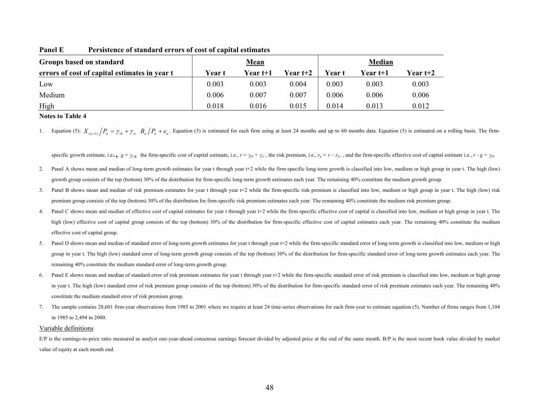
48

Panel E Persistence of standard errors of cost of capital estimates Groups based on standard Mean Median errors of cost of capital estimates in year t Year t Year t+1 Year t+2 Year t Year t+1 Year t+2 Low 0.003 0.003 0.004 0.003 0.003 0.003 Medium 0.006 0.007 0.007 0.006 0.006 0.006 High 0.018 0.016 0.015 0.014 0.013 0.012 Notes to Table 4

1. Equation (5): ( 1) 0 1 i t it i i it it itX P B P eγ γ+ = + + . Equation (5) is estimated for each firm using at least 24 months and up to 60 months data. Equation (5) is estimated on a rolling basis. The firm-

specific growth estimate, i.e., g = γj1, the firm-specific cost of capital estimate, i.e., r = γj0 + γj1 , the risk premium, i.e., rp = r – rf,, , and the firm-specific effective cost of capital estimate i.e., r - g = γj0.

2. Panel A shows mean and median of long-term growth estimates for year t through year t+2 while the firm-specific long-term growth is classified into low, medium or high group in year t. The high (low)

growth group consists of the top (bottom) 30% of the distribution for firm-specific long-term growth estimates each year. The remaining 40% constitute the medium growth group.

3. Panel B shows mean and median of risk premium estimates for year t through year t+2 while the firm-specific risk premium is classified into low, medium or high group in year t. The high (low) risk

premium group consists of the top (bottom) 30% of the distribution for firm-specific risk premium estimates each year. The remaining 40% constitute the medium risk premium group.

4. Panel C shows mean and median of effective cost of capital estimates for year t through year t+2 while the firm-specific effective cost of capital is classified into low, medium or high group in year t. The

high (low) effective cost of capital group consists of the top (bottom) 30% of the distribution for firm-specific effective cost of capital estimates each year. The remaining 40% constitute the medium

effective cost of capital group.

5. Panel D shows mean and median of standard error of long-term growth estimates for year t through year t+2 while the firm-specific standard error of long-term growth is classified into low, medium or high

group in year t. The high (low) standard error of long-term growth group consists of the top (bottom) 30% of the distribution for firm-specific standard error of long-term growth estimates each year. The

remaining 40% constitute the medium standard error of long-term growth group.

6. Panel E shows mean and median of standard error of risk premium estimates for year t through year t+2 while the firm-specific standard error of risk premium is classified into low, medium or high group

in year t. The high (low) standard error of risk premium group consists of the top (bottom) 30% of the distribution for firm-specific standard error of risk premium estimates each year. The remaining 40%

constitute the medium standard error of risk premium group.

7. The sample contains 28,601 firm-year observations from 1985 to 2001 where we require at least 24 time-series observations for each firm-year to estimate equation (5). Number of firms ranges from 1,104

in 1985 to 2,494 in 2000.

Variable definitions E/P is the earnings-to-price ratio measured as analyst one-year-ahead consensus earnings forecast divided by adjusted price at the end of the same month. B/P is the most recent book value divided by market

value of equity at each month end.

49

Table 5: Association of Risk Premium and Growth Rate with Firm-specific Risk and Growth Characteristics Panel A: Determinants of risk premium using equation (5) -- Dependent variable = rp(epbm)

Beta ln(MV) ln(BV/MV) ln(D/MV)

Mean 0.22 -0.01 0.18 -0.05 T-statistics (3.28) (-0.73) (4.22) (-3.10)

Number of positive years (significant years) 13(4) 6(2) 15(3) 3(1)

Number of negative years (significant years) 4(0) 11(3) 2(0) 14(2) Panel B: Determinants of risk premium using OJ model -- Dependent variable = rp(oj)

Beta ln(MV) ln(BV/MV) ln(D/MV)

Mean 1.28 -0.34 0.22 0.26 T-statistics (9.79) (-7.02) (2.00) (7.48) Number of positive years (significant years) 17(16) 1(0) 9(7) 17(16) Number of negative years (significant years) 0(0) 16(15) 8(2) 0(0) Panel C: Determinants of growth rate-- Dependent variable = g (epbm)

Analyst growth Sales growth Income growth

Mean 0.074 0.039 0.003

T-statistics (2.63) (4.34) (6.73)

Number of positive years (significant years) 13(10) 14(12) 16(14)

Number of negative years (significant years) 4(2) 3(1) 1(0) Notes to Table 5

1. Equation (5): ( 1) 0 1 i t it i i it it itX P B P eγ γ+ = + + . Equation (5) is estimated for each firm using at least 24 months and up to 60 months data. Equation (5) is estimated on a rolling basis. The firm-

specific growth estimate, i.e., g = γj1, the firm-specific cost of capital estimate, i.e., r = γj0 + γj1 the risk premium, i.e., rp = r – rf,, and the firm-specific effective cost of capital estimate i.e., r - g = γj0.

50

2. Panel A shows the result of year-by-year regressions of the firm-specific risk premium obtained using equation (5) on risk characteristics.

3. Panel B shows the result of year-by-year regressions of the firm-specific risk premium obtained using the OJ model on risk characteristics.

4. Panel A shows the result of year-by-year regressions of the firm-specific long-term growth estimate using equation (5) on firm-specific growth measures.

5. The mean coefficients are obtained from 17 annual regressions. T-statistics are computed using Fama-MacBeth (1973) procedure.

6. Number of positive years (significant years) indicates the number of years with positive (positive and significant) coefficients. Number of negative years (significant years) indicates the number of years

with negative (negative and significant) coefficients.

7. The sample contains 20,169 firm-year observations from 1985 to 2001. Number of firms ranges from 848 in 1985 to 1,571 in 1991. Variable definitions E/P is the earnings-to-price ratio measured as analyst one-year-ahead consensus earnings forecast divided by adjusted price at the end of the same month. B/P is the most recent book value divided by market

value of equity at each month end. BV/MV is the book-to-market ratio calculated as the book value of year t-1 divided by the market value of equity at the end of December of year t-1. Beta is computed using a

60 months rolling window before the date of measurement. Ln(MV) is the log of market value of equity. Market value of equity is calculated as price times shares outstanding at the end of June in year t.

Ln(BV/MV) is the log of book-to-market ratio calculated as the book value of year t-1 divided by the market value of equity at the end of December of year t-1. Ln(D/MV) is the debt-to-market value of equity

ratio calculated using the long-term debt of year t-1 divided by the market value of equity at the end of December of year t-1Analyst growth is the analysts’ long-term earnings growth forecast obtained from

I/B/E/S. Sales growth is computed as the difference of sales (Compustat #12) between year t and year t-1 divide by the sales in year t-1. Earnings growth is computed relative to the prior year using earnings

before extraordinary items (Compustat #18). rp(epbm) is the risk premium estimate obtained from equation (5). rp(oj) is the risk premium estimate obtained from the Ohlson-Juettner model (see Gode and

Mohanram, 2003). g (epbm) is the long-term growth estimate obtained from equation (5).

51

Table 6: Future returns and cost of capital estimates Panel A: OLS regression of future returns on cost of capital estimates

Dependent variable One-year-ahead

Returns without R0

Two-year-ahead returns without R0

One-year-ahead returns with R0

rp(epbm) rp(oj) rp(epbm) rp(oj) rp(epbm) R0 rp(oj) R0 Mean 0.23 -0.37 0.03 -0.30 0.15 0.07 -0.36 0.08 t-stat (1.56) (-1.47) (0.19) (-1.08) (1.06) (3.03) (-1.47) (3.65) Number of positive years (significant years) 13(9) 6(5) 9(6) 7(5) 11(7) 12(8) 6(4) 14(12) Number of negative years (significant years) 4(4) 11(9) 8(3) 10(8) 6(4) 5(2) 11(10) 3(1) Panel B: WLS regression of future returns on cost of capital estimates Dependent variable One-year-ahead returns without

R0 Two-year-ahead returns

without R0 One-year-ahead returns

with control rp(epbm) rp(epbm) rp(epbm) R0 Mean 0.40 0.28 0.30 0.06 t-stat (2.17) (1.77) (1.87) (2.62) Number of positive years (significant years) 12(11) 11(7) 11(9) 11(9) Number of negative years (significant years) 4(2) 4(2) 5(3) 5(3) Notes to Table 6

1. Equation (5): ( 1) 0 1 i t it i i it it itX P B P eγ γ+ = + + . Equation (5) is estimated for each firm using at least 24 months and up to 60 months data. Equation (5) is estimated on a rolling basis. The firm-

specific growth estimate, i.e., g = γj1, the firm-specific cost of capital estimate, i.e., r = γj0 + γj1,the risk premium, i.e., rp = r – rf, , and the firm-specific effective cost of capital estimate i.e., r - g = γj0.

2. Panel A shows Ordinary Least Square (OLS) results of cross-sectional yearly regressions from regressing one-year-ahead and two-year ahead returns on cost of capital measure obtained using equation (5)

and the Ohlson-Juettner model.

3. Panel B shows Weighted Least Square (WLS) results of cross-sectional yearly regressions from regressing one-year-ahead and two-year ahead returns on cost of capital measure obtained using EPBM

model with and without controls. The weights for WLS are the inverse of standard errors of firm-specific cost of capital estimates.

4. The mean coefficients are obtained from 17 annual regressions. T-statistics are computed using Fama-MacBeth (1973) procedure.

52

5. Number of positive years (significant years) indicates the number of years with positive (positive and significant) coefficients. Number of negative years (significant years) indicates the number of years

with negative (negative and significant) coefficients.

6. The sample contains 28,601 firm-year observations from 1985 to 2001. Number of firms ranges from 1,104 in 1985 to 2,494 in 2000.

Variable definitions E/P is the earnings-to-price ratio measured as analyst one-year-ahead consensus earnings forecast divided by adjusted price at the end of the same month. B/P is the most recent book value divided by market

value of equity at each month end. R0 is the stock return measured from July to June during which the cost of capital measure is computed. rp(epbm) is the risk premium estimate obtained from equation (5). rp(oj)

is the risk premium estimate obtained from the Ohlson-Juettner model (see Gode and Mohanram, 2003).

53

Table 7: Application of the firm-specific growth and cost of capital estimates – the value-glamour anomaly Panel A: Long-term growth

Mean Difference= Median Difference= BV/MV group in year t Year t Year t+1 Year t+2 Year t-Year t+1 (p-value) Year t Year t+1 Year t+2 Year t-Year t+2 (p-value) Low 0.133 0.125 0.117 0.016 (<0.0001) 0.126 0.116 0.107 0.019 (<0.0001) Medium 0.080 0.077 0.076 0.004 (<0.0001) 0.082 0.079 0.078 0.004 (<0.0001) High 0.034 0.039 0.047 -0.013 (<0.0001) 0.030 0.038 0.050 -0.020 (<0.0001) Panel B: Risk-premium

Mean Difference= Median Difference= BV/MV group in year t Year t Year t+1 Year t+2 Year t-Year t+1 (p-value) Year t Year t+1 Year t+2 Year t-Year t+2 (p-value) Low 0.101 0.098 0.096 0.005 (<0.0001) 0.087 0.084 0.082 0.005 (0.11) Medium 0.065 0.066 0.068 -0.003 (0.015) 0.063 0.064 0.066 -0.003 (<0.0001) High 0.048 0.050 0.056 -0.008 (<0.0001) 0.045 0.049 0.054 -0.009 (<0.0001) Panel C: Effective cost of capital

Mean Difference= Median Difference= BV/MV group in year t Year t Year t+1 Year t+2 Year t-Year t+1 (p-value) Year t Year t+1 Year t+2 Year t-Year t+2 (p-value) Low 0.021 0.024 0.026 -0.005 (0.007) 0.020 0.022 0.025 -0.005 (<0.0001) Medium 0.039 0.039 0.039 0.000 (0.492) 0.033 0.034 0.034 -0.001 (0.001) High 0.066 0.062 0.056 0.010 (<0.0001) 0.059 0.053 0.048 0.011 (<0.0001) Panel D: BV/MV value

Mean Difference= Median Difference= BV/MV group in year t Year t Year t+1 Year t+2 Year t-Year t+1 (p-value) Year t Year t+1 Year t+2 Year t-Year t+2 (p-value) Low 0.239 0.287 0.348 -0.109 (<0.0001) 0.243 0.260 0.287 -0.044 (<0.0001) Medium 0.525 0.556 0.591 -0.066 (<0.0001) 0.514 0.525 0.529 -0.015 (0.935) High 3.965 4.304 4.422 -0.457 (0.551) 0.970 0.947 0.873 0.097 (<0.0001)

54

Notes to Table 7

1. Equation (5): ( 1) 0 1 i t it i i it it itX P B P eγ γ+ = + + . Equation (5) is estimated for each firm using at least 24 months and up to 60 months data. Equation (5) is estimated on a rolling basis. The firm-

specific growth estimate, i.e., g = γj1, the firm-specific cost of capital estimate, i.e., r = γj0 + γj1 ,the risk premium, i.e., rp = r – rf, , and the firm-specific effective cost of capital estimate i.e., r - g = γj0.

2. The high (low) book-to-market group consists of the top (bottom) 30% of the book-to-market distribution each year. The remaining 40% constitute the medium book-to-market group.

3. Panel A shows mean and median of long-term growth estimates for years t through t+2 for firms classified as low, medium or high book-to-market group in year t.

4. Panel B shows mean and median of risk premium estimates for years t through t+2 for firms classified as low, medium or high book-to-market group in year t.

5. Panel C shows mean and median of effective cost of capital estimates for years t through t+2 for firms classified as low, medium or high book-to-market group in year t.

6. Panel D shows mean and median of book-t-market ratios for years t through t+2 for firms classified as low, medium or high book-to-market group in year t.

7. The sample contains 28,601 firm-year observations from 1985 to 2001. Number of firms ranges from 1,104 in 1985 to 2,494 in 2000.

Variable definitions E/P is the earnings-to-price ratio measured as analyst one-year-ahead consensus earnings forecast divided by adjusted price at the end of the same month. B/P is the most recent book value divided by market

value of equity at each month end. BV/MV is the book-to-market ratio calculated as the book value of year t-1 divided by the market value of equity at the end of December of year t-1.