Romero Mata, Omar.pdf
247
Frontpage for master thesis Faculty of Science and Technology Decision made by the Dean October 30 th 2009 Faculty of Science and Technology MASTER’S THESIS Study program/ Specialization: Master in Offshore Technology / Subsea Technology Spring semester, 2010 Open / Restricted access Writer: Omar Romero Mata ………………………………………… (W riter’s signature) Faculty supervisor: Ove Tobias Gudmestad External supervisor(s): Title of thesis: Model for economical analysis of oil and gas deepwater production concepts / Comparisons of Life Cycle Cost of Subsea Production Systems vs. Floating Structures with dry wellheads. Credits (ECTS): Thirty (30 ECTS) Key words: Deep Water, Dry tree, Wet tree, Concept Selection, Mexico, Pages: 106 (Including this frontpage, abstract and acknowledgement ) + enclosure: ………… Stavanger, June 14th/ 2010 Date/year
Transcript of Romero Mata, Omar.pdf
Frontpage for master thesis Faculty of Science and Technology
Decision made by the Dean October 30th 2009
Faculty of Science and Technology
MASTER’S THESIS
Study program/ Specialization: Master in Offshore Technology / Subsea Technology
Spring semester, 2010
Open / Restricted access
Writer: Omar Romero Mata
…………………………………………
(Writer’s signature) Faculty supervisor: Ove Tobias Gudmestad External supervisor(s): Title of thesis: Model for economical analysis of oil and gas deepwater production concepts / Comparisons of Life Cycle Cost of Subsea Production Systems vs. Floating Structures with dry wellheads. Credits (ECTS): Thirty (30 ECTS) Key words: Deep Water, Dry tree, Wet tree, Concept Selection, Mexico,
Pages: 106 (Including this frontpage,
abstract and acknowledgement ) + enclosure: …………
Stavanger, June 14th/ 2010 Date/year
I
Abstract: The scope of the work was to create a model that will allow the comparison of Life Cycle
Costs (LCC) for subsea production systems and floating structures with dry wellheads for the
Mexican territorial waters of the Gulf of Mexico.
To give validity to the model, an empirical comparison on the resulting recovery factor based
on data of the US Gulf of Mexico was included. This comparison is intended to answer ¿Is
there a significant difference in the recovery factor when is used the dry tree vs. the wet tree
concept solutions?
The model proposed integrates a number of already published models done by academics, the
industry and governments. Also, it was found that the activity in deep water offshore Mexico
is having place in a region with an evident lack of preexisting infrastructure. Hence it is
proposed in the model that new offshore structures shall have an added value for comparison
purposes
Two hypothetical projects (three different concepts for each project) of field development,
based in public information released by PEMEX, are assessed.
Conclusions and recommendations are made to increase the possibilities of feasible future
field development and efficient depletion of the hydrocarbons located in Mexican deepwater.
II
Acknowledgement: This thesis has represented a large amount of challenging work that finally has been
completed. It also increased my knowledge and extended much more my curiosity about the
oil and gas industry, which makes me understand in a much better way the complexity and
scope of decisions that are taken when the field development projects are committed.
I hope that this work will contribute to the discussion and further analysis that increase the
possibilities of oil and gas field development and ensure an efficient depletion of hydrocarbon
resources located in Mexican deepwater. Most of all, is my best wish that these possibilities
will be in the wellbeing of the Mexican population
This work might have not been possible without the valuable and encouraging participation of
the advisor for this master thesis the professor Ove Tobias Gudmestad. The advice and
commitment of the professor Jonas Odland as well as the feedback received from the
professors Tore Markeset and Arnfinn Nergaard were very important.
An acknowledgement is needed also to an important sponsor for the writing of this thesis, the
“Instituto de Financiamiento e Información para la Educación” from Guanajuato Mexico.
Big thanks to my parents Jose Jesus and Maria Esther and for all my brothers and sisters for
their support and encouragement.
Finally and most important, this work is dedicated to my wife Olena and my daughter Elena
Valentina whom represents my major motivation.
Page 1 of 103
Table of Contents 1. Scope of the work ........................................................................................................................... 4
2. Expected benefits of this work ........................................................................................................ 5
FIRST PART: THEORETICAL BACKGROUND .......................................................................................... 6
3. State of the art in production of oil and gas in deep water ............................................................ 7
3.1. Sizing the global industry of construction of subsea oil and gas facilities. ........................ 7
3.2. Subsea deep water record. ................................................................................................ 7
3.3. Main operative challenges. ................................................................................................ 8
3.4. Risks in projects in deep water........................................................................................... 9
4. Offshore field development .......................................................................................................... 10
4.1 Origins of oil and gas resources ........................................................................................ 11
4.2. Hydrocarbon products ..................................................................................................... 11
4.3 Value chain in oil and gas .................................................................................................. 13
4.4 Phases and decision gates planning the offshore field development ............................... 15
4.4.1 Pre‐concession or prelease work ............................................................................... 17
4.4.2 Concession round. ...................................................................................................... 19
4.4.3 Exploration activities .................................................................................................. 20
4.4.4. Appraisal and development planning ....................................................................... 22
5. Concept Selection and Life Cycle Cost .......................................................................................... 26
5.1 Concept selection purpose and organization .................................................................... 26
5.2 Factors influencing the concept selection. ....................................................................... 27
5.2.1 Reservoir characteristics ............................................................................................ 29
5.2.2. Fluid characteristics ................................................................................................... 30
5.2.3. Reservoir uncertainty (Risk) ...................................................................................... 31
5.2.4. Location characteristics ............................................................................................. 32
5.2.5 Regional development status ..................................................................................... 33
5.2.6. Technical development status. ................................................................................. 33
5.2.7 Politics ........................................................................................................................ 33
5.2.8. Schedule .................................................................................................................... 33
5.2.9. Equipment availability ............................................................................................... 34
5.2.10. Market availability ................................................................................................... 34
5.2.11. Economics ............................................................................................................... 34
5.3 Life Cycle Cost in concept selection processes ................................................................. 34
Page 2 of 103
6. Production concepts for offshore field development in deepwater ............................................ 40
6.1 Technological assessment of the subsea production systems (wet tree solutions) ......... 41
6.1.1. Subsea Processing ..................................................................................................... 41
6.1.2 Flow Assurance ........................................................................................................... 43
6.1.3. Well Intervention ...................................................................................................... 43
6.1.4. Long term well monitoring ........................................................................................ 44
6.1.5. Factors affecting ultimate recovery .......................................................................... 44
6.1.6. Risk, safety and environmental concerns ................................................................. 44
6.1.7. Technology development and transfer. .................................................................... 44
6.1.8. Reliability of production and control of subsea systems .......................................... 45
6.1.9. A flexible concept. Tieback to floating or fixed offshore installations or tie back to shore. ................................................................................................................................... 45
6.1.10 Marine operations. ................................................................................................... 47
6.2 Technological assessment of floating structures (dry tree solutions) .............................. 47
6.2.1 State of the art of developed fields using SPAR. ........................................................ 48
6.2.2 Description of the SPAR floating system. ................................................................... 48
6.2.3. Benefits and challenges of the SPAR’s concept. ....................................................... 49
6.2.1 State of the art of developed fields using TLP´s. ........................................................ 50
6.2.4. Description of the concept of the TLP´s systems. ..................................................... 50
6.2.5. Benefits and challenges for the TLP concept. ........................................................... 54
SECOND PART: DEVELOPMENT, CONCLUSIONS AND RECOMENDATIONS ....................................... 55
7. Discussion on the recovery factor Dry vs. Wet Tree ..................................................................... 56
7.1 Empirical analysis of recovery factors in deepwater US Gulf of Mexico for dry tree vs. wet tree field development solutions. ........................................................................................... 58
7.1.1. Purpose ..................................................................................................................... 58
7.1.2 Methodology .............................................................................................................. 59
7.1.3 Results and inferences ............................................................................................... 61
7.2 Multifactorial models for the prediction of the recovery factor. ..................................... 63
7.2.1 The Reservoir Complexity Index from the Norwegian petroleum directorate. ......... 64
7.2.2 Inferences about the Reservoir Complexity Index from the Norwegian petroleum directorate on the performance of dry and wet tree solutions. ......................................... 64
8. Models presentation ..................................................................................................................... 67
8.1 Oil and Gas Exploration Economic Model of the Nova Scotia Department of Energy ...... 67
8.2 Empirical Cost Model for TLP’s and SPAR’s CAPEX. .......................................................... 67
8.3 Goldsmith Models for OPEX, RAMEX and RISKEX. ............................................................ 71
Page 3 of 103
8.4 Value added of a floating structure acting as a Hub ......................................................... 71
9.0 Case Analysis. .............................................................................................................................. 73
9.1 General basis for analysis. ................................................................................................. 75
9.2 Scenario I: Deep water stand alone gas field .................................................................... 77
9.2.1 Basis for analysis ........................................................................................................ 77
9.2.2 Alternative concepts to test ....................................................................................... 77
9.2.3 Results ........................................................................................................................ 79
9.3 Scenario II: Deep water array of gas and condensate fields in proximity ......................... 83
9.3.1 Basis for analysis ........................................................................................................ 84
9.3.2 Alternative concepts to test ....................................................................................... 84
9.3.3 Results ........................................................................................................................ 88
9.4. Deep water heavy and extra heavy oil fields. .................................................................. 91
9.5. Conclusions ................................................................................................................................ 92
10. General Conclusions .................................................................................................................... 94
10.1 On the discussion on the recovery factor Dry vs. Wet Tree ........................................... 94
10.2 On the Case Analysis ....................................................................................................... 95
10.3 Recommendations .......................................................................................................... 97
References ......................................................................................................................................... 98
Enclosure:
• Annex A: Empirical research on the behavior of the investment in exploration for oil and gas in the Norwegian Continental Shelf
• Annex B: Requirements, activities and products of the development planning phases
• Annex C: Field development examples
• Annex D: Marine operations
• Annex E: Extended results of the recovery factor data analysis for oil and gas fields in the U.S. Gulf of Mexico.
• Annex F: Nova Scotia Model Description, reverse modeling of the excel file.
• Annex G: Design Basis for the Case Analysis
Page 4 of 103
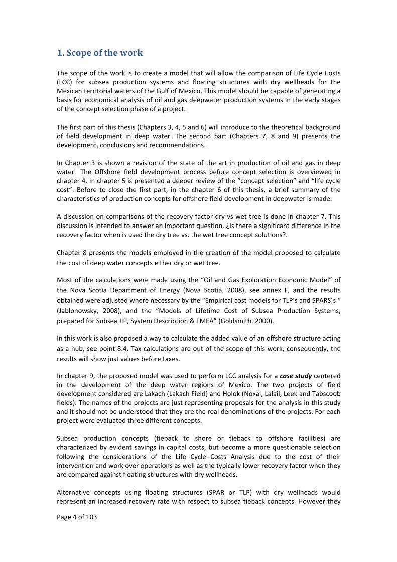
1. Scope of the work The scope of the work is to create a model that will allow the comparison of Life Cycle Costs (LCC) for subsea production systems and floating structures with dry wellheads for the Mexican territorial waters of the Gulf of Mexico. This model should be capable of generating a basis for economical analysis of oil and gas deepwater production systems in the early stages of the concept selection phase of a project. The first part of this thesis (Chapters 3, 4, 5 and 6) will introduce to the theoretical background of field development in deep water. The second part (Chapters 7, 8 and 9) presents the development, conclusions and recommendations. In Chapter 3 is shown a revision of the state of the art in production of oil and gas in deep water. The Offshore field development process before concept selection is overviewed in chapter 4. In chapter 5 is presented a deeper review of the “concept selection” and “life cycle cost”. Before to close the first part, in the chapter 6 of this thesis, a brief summary of the characteristics of production concepts for offshore field development in deepwater is made. A discussion on comparisons of the recovery factor dry vs wet tree is done in chapter 7. This discussion is intended to answer an important question. ¿Is there a significant difference in the recovery factor when is used the dry tree vs. the wet tree concept solutions?. Chapter 8 presents the models employed in the creation of the model proposed to calculate the cost of deep water concepts either dry or wet tree.
Most of the calculations were made using the “Oil and Gas Exploration Economic Model” of the Nova Scotia Department of Energy (Nova Scotia, 2008), see annex F, and the results obtained were adjusted where necessary by the “Empirical cost models for TLP’s and SPARS´s “ (Jablonowsky, 2008), and the “Models of Lifetime Cost of Subsea Production Systems, prepared for Subsea JIP, System Description & FMEA” (Goldsmith, 2000).
In this work is also proposed a way to calculate the added value of an offshore structure acting as a hub, see point 8.4. Tax calculations are out of the scope of this work, consequently, the results will show just values before taxes.
In chapter 9, the proposed model was used to perform LCC analysis for a case study centered in the development of the deep water regions of Mexico. The two projects of field development considered are Lakach (Lakach Field) and Holok (Noxal, Lalail, Leek and Tabscoob fields). The names of the projects are just representing proposals for the analysis in this study and it should not be understood that they are the real denominations of the projects. For each project were evaluated three different concepts. Subsea production concepts (tieback to shore or tieback to offshore facilities) are characterized by evident savings in capital costs, but become a more questionable selection following the considerations of the Life Cycle Costs Analysis due to the cost of their intervention and work over operations as well as the typically lower recovery factor when they are compared against floating structures with dry wellheads. Alternative concepts using floating structures (SPAR or TLP) with dry wellheads would represent an increased recovery rate with respect to subsea tieback concepts. However they
Page 5 of 103
are also associated with high investments costs and a huge competence challenge for the skills in the construction, installation, and operation management of these facilities. For the case analysis it was found that the activity in deep water offshore Mexico is having place in a region with an evident lack of preexisting infrastructure. This fact makes it important to develop a network of facilities that should increase the feasibility of development in the future. Hence it is proposed here that additional offshore structures shall have an added value for comparison purposes. This added value will be calculated by doing an evaluation of NPV for the prospects that could be developed if the facility would be in place already.
This work closes with conclusions and recommendations that in opinion of the author might increase the possibilities of development and ensure efficient depletion of hydrocarbon resources located in Mexican deepwater.
2. Expected benefits of this work PEMEX Exploración and Producción (PEP) is developing the field Lakach in the Mexican territorial waters of the Gulf of Mexico. The Lakach field is the first offshore field to be developed in deep water by PEMEX and is a part of an extensive effort by this National Company to fulfill the exploratory works and field development in basins that before were not considered to be commercially feasible. A subsea tieback to shore has already been revealed by PEP as the selected concept for this development. However, there are many other prospects of development in the adjacent area that are already being included in the portfolio of exploration and that in the future could be the subject of further studies.

Page 6 of 103
FIRST PART: THEORETICAL BACKGROUND
Page 7 of 103
3. State of the art in production of oil and gas in deep water
3.1. Sizing the global industry of construction of subsea oil and gas facilities.
The subsea technology is not the only way that can reach deep water, as we will see along this work, also the floating structures that use dry completion can be a sound solution for field development in deep water. However, subsea systems are important because in many cases they are the only option to develop fields and alone or in conjunction with floating structures represent the most extendedly used solution for deep water.
The construction of production facilities of oil and gas using subsea technology is expected to be one of the most dynamically developed industries in the next years. According to “Infield Energy Analysts” (Offshore, 02‐09‐2009), the forecasted total global subsea sector´s expenditure will exceed $80 billion USD over the period 2009 through to 2013.This amount almost doubles the expenditure in subsea equipment, drilling and completion that were accounted for $46 billion USD the past five years.
The biggest operators, based upon the number of subsea valve trees expected to be started up within the next five years are:
1. Petrobras 374 2. Shell 244 3. Total 237 4. Chevron 236 5. BP 229 6. ExxonMobil 215 7. Statoil 194
In total 3,222 subsea valve trees are expected to begin their operations in this period.
3.2. Subsea deep water record.
The record in drilling and completion is hold by Shell Oil Co. This company has reached 9,356 ft (2,852 m) below the water's surface in the Silvertip field at the Perdido Development project in the Gulf of Mexico (Offshore, 12‐02‐2008).
• Location: Gulf of Mexico, US
• Depth: ~2,380 metres
• Interests: Shell 35% (operator), Chevron 37.5%, BP 27.5%
• Fields: Great White, Tobago, Silvertip
• Peak Production: 130 kboe/d [API: 18‐40]
• Key contractors: Technip, Kiewit, FMC Technologies, Heerema, Marine Contractors.
Page 8 of 103
Technology:
Perdido, moored in approximately 2,380m of water, will be the world’s deepest Direct Vertical Access Spar. The spar will act as a hub that will enable the development of three fields – Great White, Tobago, and Silvertip – and it will gather process and export production capability within a 48km radius. Tobago, in 2,925m of water, will be the world’s deepest subsea completion.
However, Deep water is not only good news. Petroleos Mexicanos (PEMEX) is a particular case of a national oil and gas company that is planned to start the operation of projects in deep water in the first half of the 2010’s. This company has identified operative challenges and risks that will be enounced next (PEMEX, 2008).
3.3. Main operative challenges.
Among many others these can be pointed to:
Marine currents and waves: strong marine current and waves induce the movement of structures and pipeline vibrations resulting in fatigue in the components of the drilling and production equipment.
The temperature changes, due to the different degrees of temperature between the surface and the drilled sub seabed formations make the pumping of the drilling fluid to become complex. Also these low temperatures alter the properties of the cement utilized to secure the casing of the well.
Critical aspects of drilling at the start up: During the drilling across shallow formations, the water flows are at high‐pressure, there are also gas flows and therefore the pressures are usually abnormal.
Remote Operation of subsea installation must be made through R.O.V s, since human beings cannot reach great depths.
High costs involved: the fields need to be developed with fewer wells than the traditionally employed in the shallow waters. The conditions usually demand highly deviated and horizontal wells to ensure the flow of oil.
Subsea facilities and equipment: the application of new technologies is required to make possible the flow assurance either to the multiphase transportation systems or for fluids separation equipment on the seabed; a high degree of automation and use of robotics is required.
Salt formations: the demand for specialized technologies for formations surveying and assessment, also the drilling of these is challenging and demand the use of new and underdevelopment technologies.
Geometry of the reservoir in deep water may be different from the familiar in shallow waters.
Page 9 of 103
3.4. Risks in projects in deep water.
Geological risks: exists due to the complexity of geological structures and the difficulty of identifying reservoirs, also in some cases the presence of saline subsurface formations deteriorate and diminish the likelihood of discovering deposits in these environments.
Operative risks: the operations are considerable more difficult to solve than in shallow water, for example:
•Flows of shallow waters and flows of gas might cause blow outs during drilling.
•Underwater tides and waves threaten the drilling facilities and the production infrastructure.
•Drilling equipment is expensive and sometimes unavailable
•Installation and maintenance of facilities is carried on at distant places and offer difficulties to access, which increase costs and delay operations.
Financial Risk: nevertheless, exposure of capital due the high costs of exploration, development and operation all‐together with instability of oil prices.
Although the technology, equipment, and materials required for the project execution in subsea field developments, including deep water, have high cost of acquisition and operation, in the most of the cases they are already commercially available worldwide.
Nevertheless and particularly more important for the operators, is necessary acquire skills and implement systems to minimize risks for the operator company and increase the added value of the investment.
Proper business process management trough the whole lifecycle undoubtedly will diminish risks as well as will increase expected economical value added of the project.
Components for the management of the business process that can be listed are:
• Asset Management
• Documentation and management of project architecture, standards, recommended practices and procedures.
• Human resources and competence management
• Health, Safety and Environmental management.
• Implementation and management of suitable information systems
• Life Cycle Cost Management
• Process Safety Management
• Project Management
• Reliability and maintenance methodologies
• Risk Management.
• Suppliers and contractors management.

Page 10 of 103
4. Offshore field development
Along the next chapters (4 and 5) some basic assumptions and facts will be reviewed on offshore field development and the concept selection in deep water. Necessarily, only an extract of all the public and available information will be mentioned due the expectancy and requisite to develop innovative content in this thesis. Wherever necessary, is suggested and encouraged to search and consult general references on this topics, a non exclusive list of suggested references is shown below:
• Class Notes of Offshore Field Development with Compendium (Odland, 2000‐2008).
• Deepwater development: A reference document for the deepwater environmental assessment Gulf of Mexico OCS (1998 through 2007)(Regg, 2006).
• Deepwater petroleum exploration & production: A nontechnical guide, (Leffler, 2003).
• Handbook of Offshore Technology, Volume I, (Chakrabarti, Editor, 2005). o Chapter 1, Historical Development of Offshore Structures (Chakrabarti et. al,
2005). o Chapter 2, Novel and Marginal Offshore Structures (Capanoglu et. al., 2005). o Chapter 6, Fixed Offshore Platform design (Karsan et. al, 2005). o Chapter 7, Floating Offshore Platform design (Halkyard et. al, 2005).
• Petroleum Engineering Handbook (Lake, Editor in chief, 2006). o Volume I General Engineering (Fanchi, Editor, 2006).
Petroleum Economics (Wright, 2006). o Volume II Drilling Engineering (Mitchell, Editor, 2006).
Introduction to Well Planning (Adams, 2006). Offshore Drilling Units (Childers, 2006).
o Volume III Facilities and construction engineering (Arnold, Editor, 2007). Oil and gas processing (Thro, 2007). Gas Treating and processing (Wichert, 2007). Piping and pipelines (Stevens and May, 2007). Offshore and Subsea Facilities (O’Connor et. al., 2007). Project Management of Surface Facilities (Kreider, 2007).
o Volume V Reservoir engineering and petrophysics (Holstein, Editor, 2007). Estimation of primary reserves of crude oil, natural gas, and
condensate (Harrel and Cronquist, 2007). Valuation of oil and gas reserves (Long, 2007).
• Oil & Gas Exploration and Production Reserves, Costs, Contracts (Babusiaux, 2004).
• Oil and gas production handbook, an Introduction to oil and gas production (Håvard, 2006).
Page 11 of 103
4.1 Origins of oil and gas resources
The terms “Oil and gas” encompasses all the different hydrocarbon compounds (those compounds made of Hydrogen and Carbon in a chemical configuration) that are useful either for combustible or for transformation purposes and that were formed from the transformation of organic substances through geophysical and geochemical processes along plenty millions of years.
The sedimentary basins are those geological layers that were formed by successive deposition of organic and inorganic masses. Along the pass of the time, those first depositional layers were subject to increasing temperatures and pressures, down in the earth, as new layers were deposited on the surface.
In some cases, the conditions deep in the earth were propitious for the decomposition and transformation of the organic masses along many thousands and millions of years. These sedimentary layers where the organic substances are changing its properties are known usually as Source Rocks.
Once the source rocks start to produce hydrocarbon compounds, those tend to climb passing trough interconnected porous in the rock and or fractures in the rock media, the path that the substances follow is refereed frequently as the migration path. Porosity is the fraction of volume of the rock that is the empty space inside of a rock formation and permeability is the ability to flow or pass trough of the fluids contained in the rocks.
The hydrocarbons substances that move from the source rock are expected to flow trough a porous and permeable media until they are stopped by a geological barrier that is above a region of porous and permeable rock that is able to store the hydrocarbon substance and make possible its economical recovery. The geological barriers are know commonly as traps and the region of porous and permeable rock where the hydrocarbon is stored is named Reservoir Rock. Depending on its form and origin the traps are classified as anticline, stratigraphic, unconformity and fault. The anticline traps are by most the more exploited so far due to their relative easiness to be located and dimensioned.
Summarizing, a promising area to be drilled for exploration (prospect) of oil and/or gas field must have:
1. A source rock reservoir rich of organic matter. 2. Enough heat and pressure along millions of years to make possible the transformation
of the organic matter to hydrocarbon substances. 3. A migration path. 4. A reservoir rock limited by a: 5. Trap system with a impermeable seal (anticline, stratigraphic, unconformity or fault).
4.2. Hydrocarbon products
Page 12 of 103
It is know that the characteristics of the reservoir are the main driver (On the decision to develop or not, on the specification of the concept and engineering, etc.) for the field develop. Those characteristics for example, will determine the type and fractional amount of the mixture of products to extract.
Hydrocarbons are not homogeneous when they are found in the subsoil. The considerable variations of the hydrocarbons in color, gravity, aroma, sulfur content and viscosity are common in petroleum from different geographical areas and even from reservoir to reservoir.
All the hydrocarbon reservoirs will differ from any others in its contents of hydrocarbons compounds and associated substances. The hydrocarbons can range in physical state from solids to gasses with water and sand as well as other impurities such as sulfur, oxygen and nitrogen.
The classification of the hydrocarbon products is based on its chemical composition. Lighter hydrocarbons (those with molecules with a small number of atoms of carbon) are usually gasses when are extracted and stay at normal atmospheric conditions.
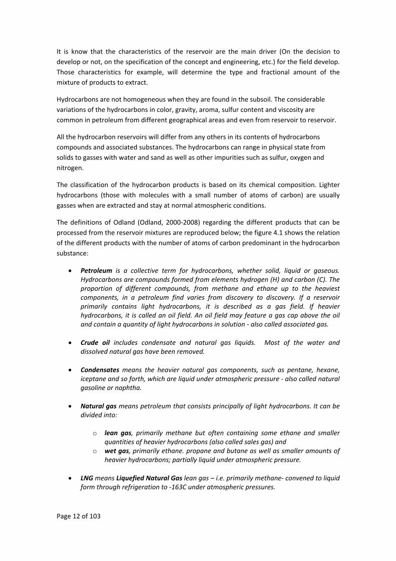
The definitions of Odland (Odland, 2000‐2008) regarding the different products that can be processed from the reservoir mixtures are reproduced below; the figure 4.1 shows the relation of the different products with the number of atoms of carbon predominant in the hydrocarbon substance:
• Petroleum is a collective term for hydrocarbons, whether solid, liquid or gaseous. Hydrocarbons are compounds formed from elements hydrogen (H) and carbon (C). The proportion of different compounds, from methane and ethane up to the heaviest components, in a petroleum find varies from discovery to discovery. If a reservoir primarily contains light hydrocarbons, it is described as a gas field. If heavier hydrocarbons, it is called an oil field. An oil field may feature a gas cap above the oil and contain a quantity of light hydrocarbons in solution ‐ also called associated gas.
• Crude oil includes condensate and natural gas liquids. Most of the water and
dissolved natural gas have been removed.
• Condensates means the heavier natural gas components, such as pentane, hexane, iceptane and so forth, which are liquid under atmospheric pressure ‐ also called natural gasoline or naphtha.
• Natural gas means petroleum that consists principally of light hydrocarbons. It can be
divided into:
o lean gas, primarily methane but often containing some ethane and smaller quantities of heavier hydrocarbons (also called sales gas) and
o wet gas, primarily ethane. propane and butane as well as smaller amounts of heavier hydrocarbons; partially liquid under atmospheric pressure.
• LNG means Liquefied Natural Gas lean gas – i.e. primarily methane‐ convened to liquid
form through refrigeration to ‐163C under atmospheric pressures.
Page 13 of 103
• LPG means Liquefied Petroleum Gas and consists primarily of propane and butane, which turn Liquid under a pressure of six to seven atmospheres. LPG is shipped in special vessels.
• Naphtha means an inflammable oil obtained by the dry distillation of petroleum.
• NGL means Natural Gas Liquids light hydrocarbons consisting mainly of ethane,
propane and butane which are liquid under pressure at normal temperature.[Odland, P.p. II “Miscellaneous term”, Hard copy compendium, 2000‐2008].
Additionally there is an alternative post processed product known as GTL (Gas to liquids). Gas to liquids refers to a refinery process to convert natural gas or other gaseous hydrocarbons into longer chained hydrocarbons such as gasoline or diesel fuel.
Figure 4.1: Classification chart of hydrocarbons and sales products [Odland, P.p. 12, Mod. 3 Petroleum resources and production, Class Notes…,2000‐2008].
4.3 Value chain in oil and gas The exploration and production of oil and gas has as main purpose to “Extract (in a cost effective, efficient, safe and as environmentally friendly as reasonable) the hydrocarbons that rely in basins under the soil surface (either in land, fresh water bodies or in the seas) and transport, process and deliver the production to a market”.
These previous facts are the basis to explain the term “value chain” that is going to be introduced in this section.
The value chain of oil and gas encompasses the chain of technological solutions that make possible to bring the hydrocarbon products from the reservoir to the final market. It is usually divided in Up‐stream, Mid‐stream and downstream. Upstream in offshore, refers to the extraction and initial processing or stabilization to transportation located offshore.
C1 C2 C3 C4 C5 C6 C7 C8 C9 C10+
Oil stable
Oil unstable
stable Condensate
unstable Condensate
LPG
NGL
Rich gas
Sales gas and LNG
C1 C2 C3 C4 C5 C6 C7 C8 C9 C10+
Page 14 of 103
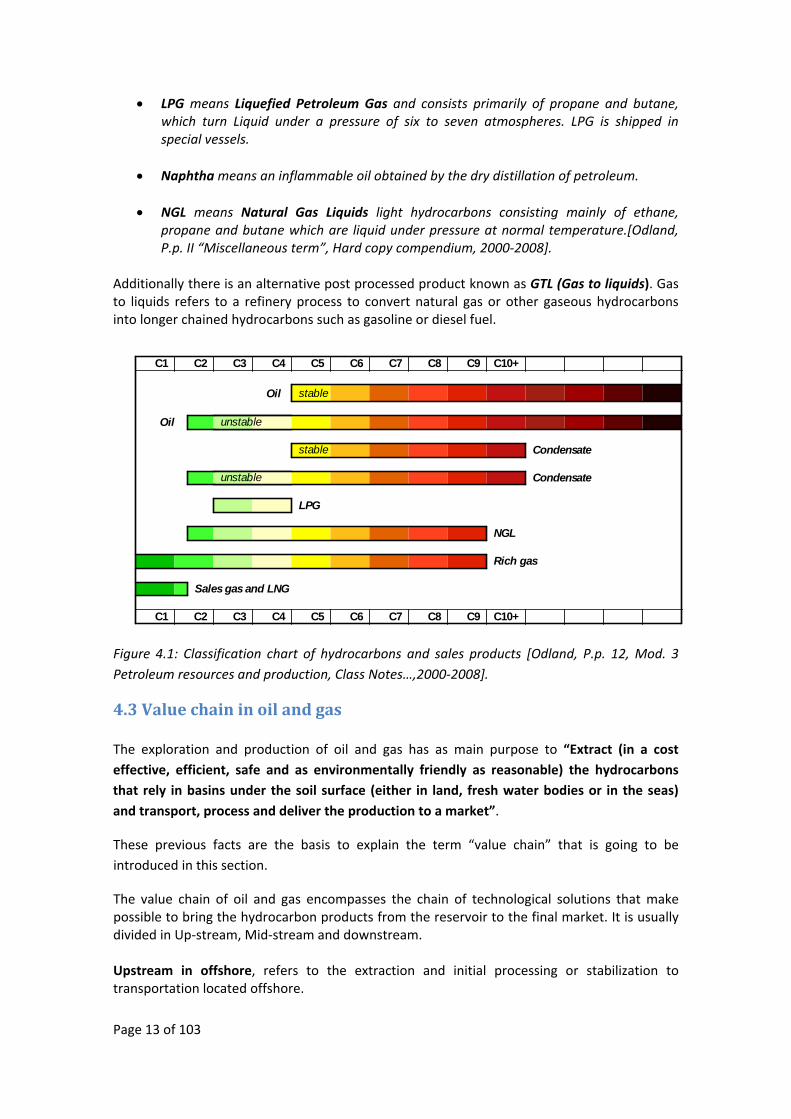
Mid stream refers to the transportation and distribution networks of technologies and process that mobilize the products from offshore to onshore processing facilities or to distribution pipeline networks to market delivery. Downstream, is mentioned to make reference to the refining and further transformation of the products received from the upstream and midstream steps. The transportation issue is closely related to the products handled and it takes an important role determining the selection of the value chain elements that will be emplaced. The goal is to optimize the life cycle value creation along the entire value chain, from the reservoir to market A field of oil plus an associated gas reservoir will have most of the possible products cataloged on the above list. Then, the handling options for the exploitation of these reservoirs would be as shown in the figure 4.2.
Figure 4.2: Products and handling options for a field of oil with associate gas.
The selection should in addition conciliate aspects entirely related to the production process such as type of hydrocarbons, geographic region, water depth, available existing assets and infrastructure, etc. There are also other non technical aspects, but not for that less important, that require attention. There are many aspects not merely related to the hydrocarbon production that must be taken in consideration. One of the most important among them is the existence of different shareholders around any oil and gas project that can have many different points of view, reacting according to them instead of focusing on the value creation. In this case a careful analysis of the value chain would help to find and conciliate the shareholders interest.
From well
stream
Asociate Gas
Processing to transport
Injection
Defer production until feasible
Enhance oil recovery
Store gas as fuel to extend production
LNG
CNG or LPG
GTL
Power
Other
Pipeline (Multiphase
flow)
Oil and condensate
Pipeline
Tanker
Page 15 of 103
4.4 Phases and decision gates planning the offshore field development
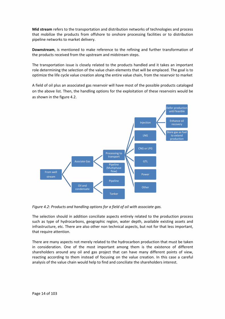
The field development is a sequential process that is carried out over several years. The figure 4.3 shows the main stages of it.
Figure 4.3: Stages of the field development.
Along each section of the field development until the start of the project execution there are several major decision gates that drive to the continuation or not of the investment. These decision gates are in place since the beginning of the pre‐concession works. It is relevant for the scope of this work to extend the discussions of the first four stages:
• Pre‐concession or prelease work
• Concession round
• Exploration
• Appraisal and development planning
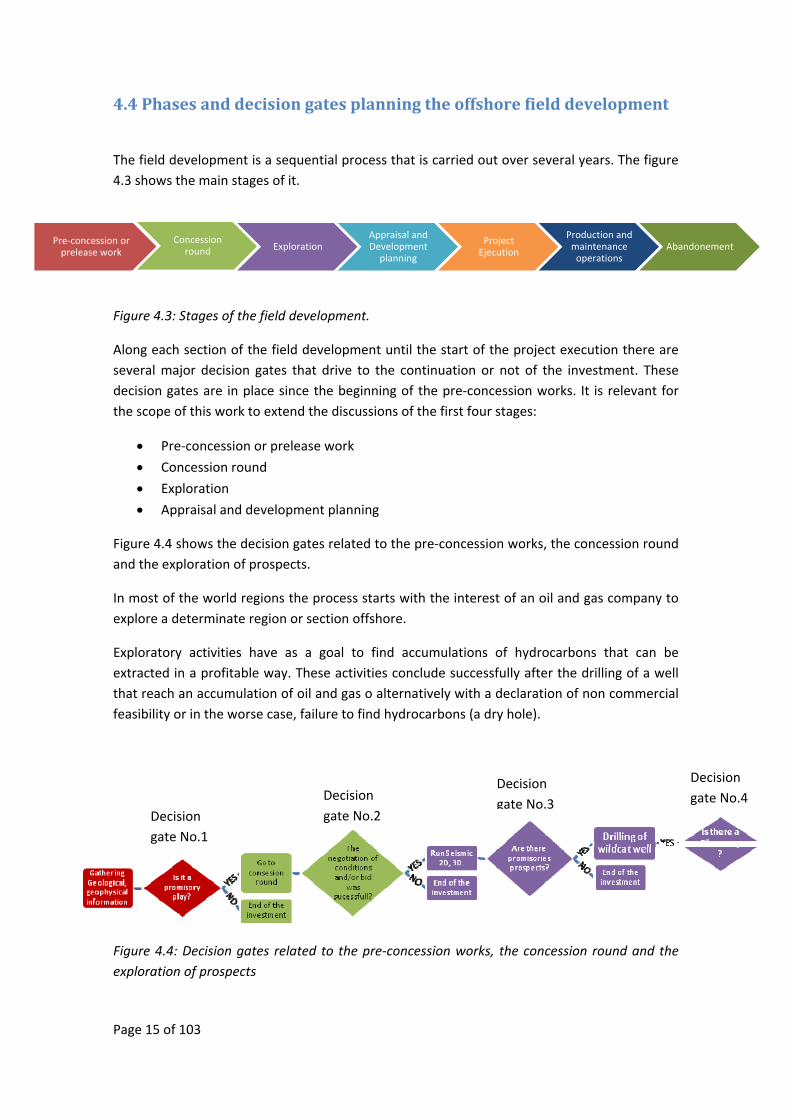
Figure 4.4 shows the decision gates related to the pre‐concession works, the concession round and the exploration of prospects.
In most of the world regions the process starts with the interest of an oil and gas company to explore a determinate region or section offshore.
Exploratory activities have as a goal to find accumulations of hydrocarbons that can be extracted in a profitable way. These activities conclude successfully after the drilling of a well that reach an accumulation of oil and gas o alternatively with a declaration of non commercial feasibility or in the worse case, failure to find hydrocarbons (a dry hole).
Figure 4.4: Decision gates related to the pre‐concession works, the concession round and the exploration of prospects
Pre‐concession or prelease work
Concession round Exploration
Appraisal and Development planning
Project Ejecution
Production and maintenance operations
Abandonement
Decision gate No.1
Decision gate No.2
Decision gate No.3
Decision gate No.4
Page 16 of 103
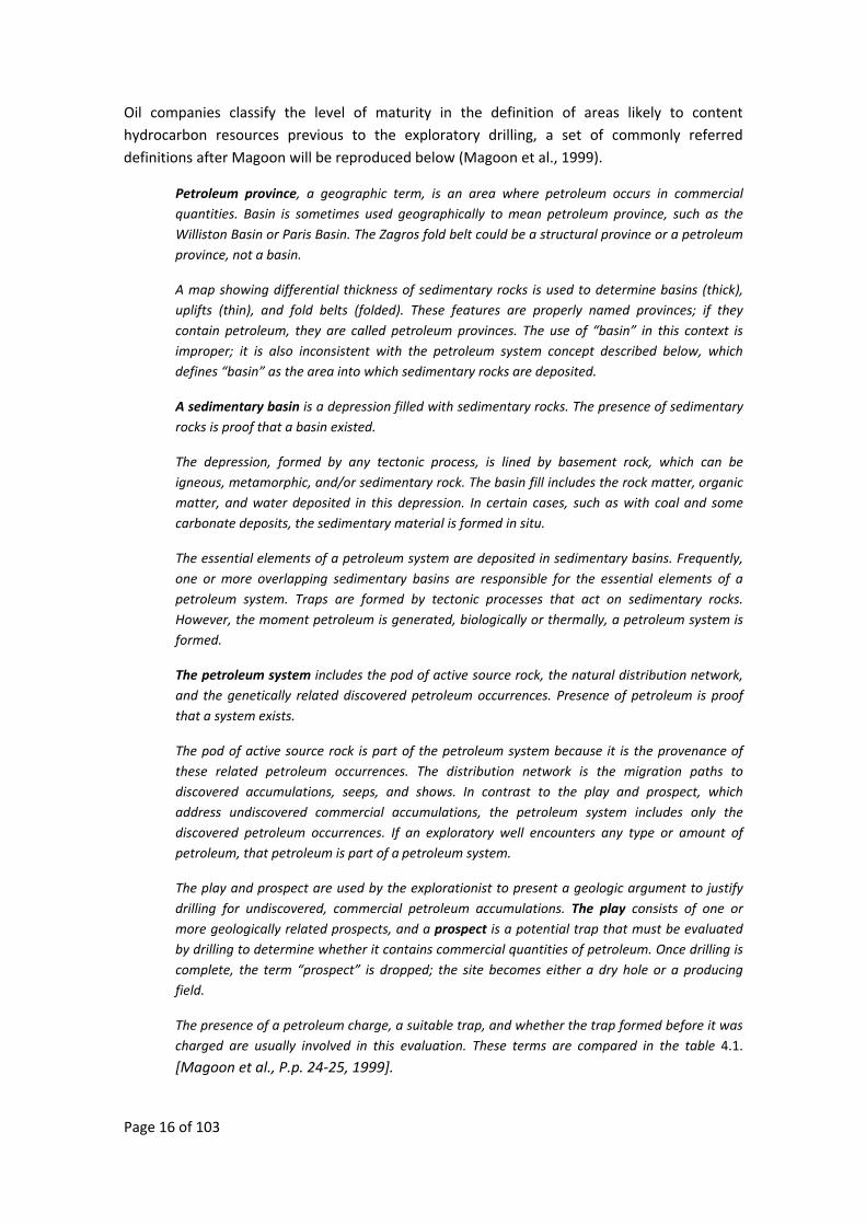
Oil companies classify the level of maturity in the definition of areas likely to content hydrocarbon resources previous to the exploratory drilling, a set of commonly referred definitions after Magoon will be reproduced below (Magoon et al., 1999).
Petroleum province, a geographic term, is an area where petroleum occurs in commercial quantities. Basin is sometimes used geographically to mean petroleum province, such as the Williston Basin or Paris Basin. The Zagros fold belt could be a structural province or a petroleum province, not a basin.
A map showing differential thickness of sedimentary rocks is used to determine basins (thick), uplifts (thin), and fold belts (folded). These features are properly named provinces; if they contain petroleum, they are called petroleum provinces. The use of “basin” in this context is improper; it is also inconsistent with the petroleum system concept described below, which defines “basin” as the area into which sedimentary rocks are deposited.
A sedimentary basin is a depression filled with sedimentary rocks. The presence of sedimentary rocks is proof that a basin existed.
The depression, formed by any tectonic process, is lined by basement rock, which can be igneous, metamorphic, and/or sedimentary rock. The basin fill includes the rock matter, organic matter, and water deposited in this depression. In certain cases, such as with coal and some carbonate deposits, the sedimentary material is formed in situ.
The essential elements of a petroleum system are deposited in sedimentary basins. Frequently, one or more overlapping sedimentary basins are responsible for the essential elements of a petroleum system. Traps are formed by tectonic processes that act on sedimentary rocks. However, the moment petroleum is generated, biologically or thermally, a petroleum system is formed.
The petroleum system includes the pod of active source rock, the natural distribution network, and the genetically related discovered petroleum occurrences. Presence of petroleum is proof that a system exists.
The pod of active source rock is part of the petroleum system because it is the provenance of these related petroleum occurrences. The distribution network is the migration paths to discovered accumulations, seeps, and shows. In contrast to the play and prospect, which address undiscovered commercial accumulations, the petroleum system includes only the discovered petroleum occurrences. If an exploratory well encounters any type or amount of petroleum, that petroleum is part of a petroleum system.
The play and prospect are used by the explorationist to present a geologic argument to justify drilling for undiscovered, commercial petroleum accumulations. The play consists of one or more geologically related prospects, and a prospect is a potential trap that must be evaluated by drilling to determine whether it contains commercial quantities of petroleum. Once drilling is complete, the term “prospect” is dropped; the site becomes either a dry hole or a producing field.
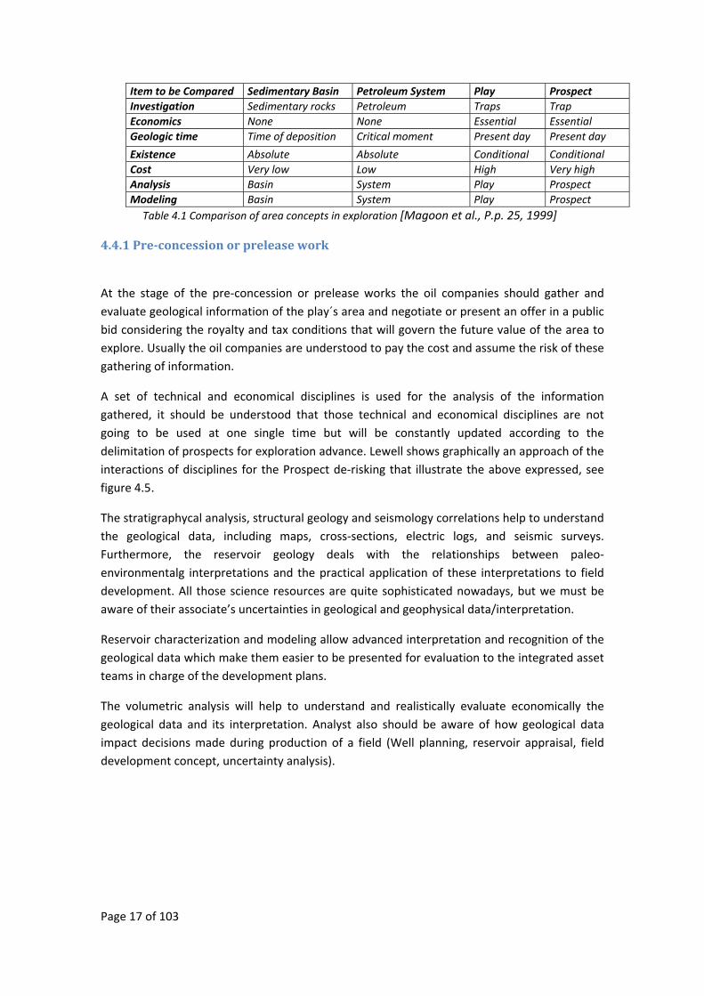
The presence of a petroleum charge, a suitable trap, and whether the trap formed before it was charged are usually involved in this evaluation. These terms are compared in the table 4.1.
[Magoon et al., P.p. 24‐25, 1999].
Page 17 of 103
Item to be Compared Sedimentary Basin Petroleum System Play ProspectInvestigation Sedimentary rocks Petroleum Traps Trap Economics None None Essential EssentialGeologic time Time of deposition Critical moment Present day Present day
Existence Absolute Absolute Conditional Conditional Cost Very low Low High Very highAnalysis Basin System Play ProspectModeling Basin System Play Prospect
Table 4.1 Comparison of area concepts in exploration [Magoon et al., P.p. 25, 1999]
4.4.1 Preconcession or prelease work
At the stage of the pre‐concession or prelease works the oil companies should gather and evaluate geological information of the play´s area and negotiate or present an offer in a public bid considering the royalty and tax conditions that will govern the future value of the area to explore. Usually the oil companies are understood to pay the cost and assume the risk of these gathering of information.
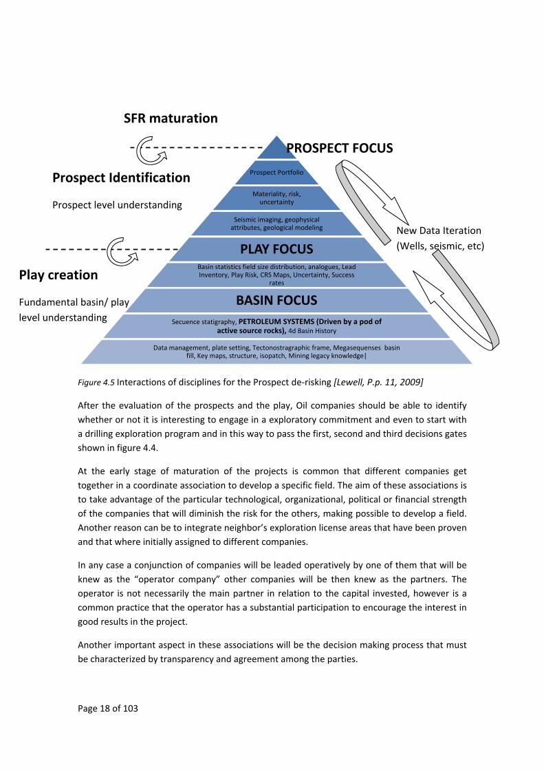
A set of technical and economical disciplines is used for the analysis of the information gathered, it should be understood that those technical and economical disciplines are not going to be used at one single time but will be constantly updated according to the delimitation of prospects for exploration advance. Lewell shows graphically an approach of the interactions of disciplines for the Prospect de‐risking that illustrate the above expressed, see figure 4.5.
The stratigraphycal analysis, structural geology and seismology correlations help to understand the geological data, including maps, cross‐sections, electric logs, and seismic surveys. Furthermore, the reservoir geology deals with the relationships between paleo‐environmentalg interpretations and the practical application of these interpretations to field development. All those science resources are quite sophisticated nowadays, but we must be aware of their associate’s uncertainties in geological and geophysical data/interpretation.
Reservoir characterization and modeling allow advanced interpretation and recognition of the geological data which make them easier to be presented for evaluation to the integrated asset teams in charge of the development plans.
The volumetric analysis will help to understand and realistically evaluate economically the geological data and its interpretation. Analyst also should be aware of how geological data impact decisions made during production of a field (Well planning, reservoir appraisal, field development concept, uncertainty analysis).
Page 18 of 103
Figure 4.5 Interactions of disciplines for the Prospect de‐risking [Lewell, P.p. 11, 2009]
After the evaluation of the prospects and the play, Oil companies should be able to identify whether or not it is interesting to engage in a exploratory commitment and even to start with a drilling exploration program and in this way to pass the first, second and third decisions gates shown in figure 4.4.
At the early stage of maturation of the projects is common that different companies get together in a coordinate association to develop a specific field. The aim of these associations is to take advantage of the particular technological, organizational, political or financial strength of the companies that will diminish the risk for the others, making possible to develop a field. Another reason can be to integrate neighbor’s exploration license areas that have been proven and that where initially assigned to different companies.
In any case a conjunction of companies will be leaded operatively by one of them that will be knew as the “operator company” other companies will be then knew as the partners. The operator is not necessarily the main partner in relation to the capital invested, however is a common practice that the operator has a substantial participation to encourage the interest in good results in the project.
Another important aspect in these associations will be the decision making process that must be characterized by transparency and agreement among the parties.
Prospect Portfolio
Materiality, risk, uncertainty
Seismic imaging, geophysical attributes, geological modeling
PLAY FOCUSBasin statistics field size distribution, analogues, Lead Inventory, Play Risk, CRS Maps, Uncertainty, Success
rates
BASIN FOCUSSecuence statigraphy, PETROLEUM SYSTEMS (Driven by a pod of
active source rocks), 4d Basin History
Data management, plate setting, Tectonostragraphic frame, Megasequenses basin fill, Key maps, structure, isopatch, Mining legacy knowledge|
PROSPECT FOCUS
New Data Iteration (Wells, seismic, etc)
Play creation
Fundamental basin/ play level understanding
SFR maturation
Prospect Identification
Prospect level understanding
Page 19 of 103
4.4.2 Concession round.
The oil companies must evaluate in this stage both technical and economical aspects of the exploration ventures. Besides the geological risks the relevance of the tax systems in the profit results must be assessed because different tax systems might drive whether there is a commercially successful discovery or not.
The oil and gas resources contained in the subsoil are entitled to be property of the nation in where these accumulations of hydrocarbons rely, with some exemptions like in the USA where a particular owner of the land is also entitled to have rights over the subsoil. The exploitation of those resources however is in the hands of oil companies, either of national, private or mixed shared ownership.
Despite some countries have National Oil Companies that operate in their own countries with monopoly practices, they are more the exception than the rule. The most of the producing countries have emplaced Fiscal Systems in order to ensure the collection of cash flow from the oil and gas ventures.
A particular analysis of those systems should be emplaced for each country or even each province or state because the set of laws and codes are different according to the geographical location of the facilities and resources. Nevertheless, it can be listed four mechanisms that the States can use to get benefits from the exploitation of resources, either emplacing all of them or just partially and with or without operative participation through National oil companies (Masseron, 1990).
• Cash Bonus: Is a form of initial payment of the company that wants a permit to do exploration. The amount can be specified by law or can be subject to negotiation. The contracts establish an initial payment that is usually done when the concession is granted and also can include a series of further payments as the time passes. The payment is irrespective of the results of the exploration activities.
• Annual Rental: A yearly payment to the owner of the land and the rights of exploitation of its subsoil. This payment is also not dependant of the results of the exploration activities.
• Royalties: A payment in exchange of the rights of exploitation due once the first oil is extracted. It can be in cash or in petroleum products and is set according in a percentage (around 12%‐15%) of the planed rate of exploitation that might be adjusted on the view of the actual production.
• Income Tax: The proportional taxes that all countries impose to commercial activities (around 50% in average for oil and gas activities).
The governments as a general rule might use the above elements in two main ways to tax the oil and gas extraction:
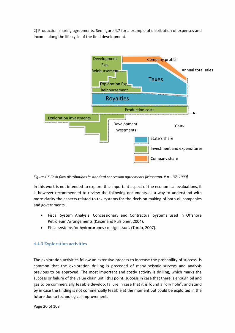
1.) Concession agreements. See figure 4.6 for a example of distribution of expenses and income along the life cycle of the field development with this tax system.
Page 20 of 103
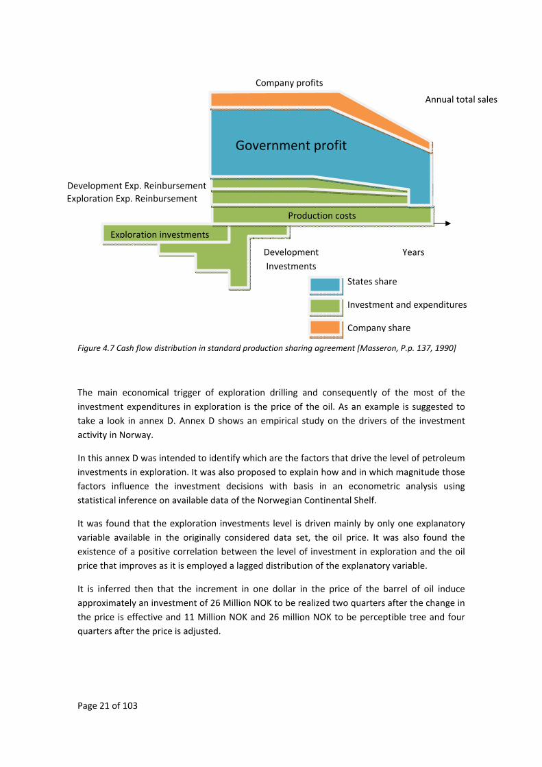
2) Production sharing agreements. See figure 4.7 for a example of distribution of expenses and income along the life cycle of the field development.
Figure 4.6 Cash flow distributions in standard concession agreements [Masseron, P.p. 137, 1990]
In this work is not intended to explore this important aspect of the economical evaluations, it is however recommended to review the following documents as a way to understand with more clarity the aspects related to tax systems for the decision making of both oil companies and governments.
• Fiscal System Analysis: Concessionary and Contractual Systems used in Offshore Petroleum Arrangements (Kaiser and Pulsipher, 2004).
• Fiscal systems for hydrocarbons : design issues (Tordo, 2007).
4.4.3 Exploration activities
The exploration activities follow an extensive process to increase the probability of success, is common that the exploration drilling is preceded of many seismic surveys and analysis previous to be approved. The most important and costly activity is drilling, which marks the success or failure of the value chain until this point, success in case that there is enough oil and gas to be commercially feasible develop, failure in case that it is found a “dry hole”, and stand by in case the finding is not commercially feasible at the moment but could be exploited in the future due to technological improvement.
Exploration investments
Production costs
Company profits
Government profit
Annual total sales
Years
State’s share
Investment and expenditures
Company share
Royalties
Development Exp.
Reinbursement
Exploration Exp. Reinbursement
Taxes
Development investments
Page 21 of 103
Figure 4.7 Cash flow distribution in standard production sharing agreement [Masseron, P.p. 137, 1990]
The main economical trigger of exploration drilling and consequently of the most of the investment expenditures in exploration is the price of the oil. As an example is suggested to take a look in annex D. Annex D shows an empirical study on the drivers of the investment activity in Norway.
In this annex D was intended to identify which are the factors that drive the level of petroleum investments in exploration. It was also proposed to explain how and in which magnitude those factors influence the investment decisions with basis in an econometric analysis using statistical inference on available data of the Norwegian Continental Shelf.
It was found that the exploration investments level is driven mainly by only one explanatory variable available in the originally considered data set, the oil price. It was also found the existence of a positive correlation between the level of investment in exploration and the oil price that improves as it is employed a lagged distribution of the explanatory variable.
It is inferred then that the increment in one dollar in the price of the barrel of oil induce approximately an investment of 26 Million NOK to be realized two quarters after the change in the price is effective and 11 Million NOK and 26 million NOK to be perceptible tree and four quarters after the price is adjusted.
Exploration investments
Production costs
Company profits
Government profit
Development Exp. Reinbursement Exploration Exp. Reinbursement
Annual total sales
Years
States share
Investment and expenditures
Company share
Development Investments
Page 22 of 103
4.4.4. Appraisal and development planning
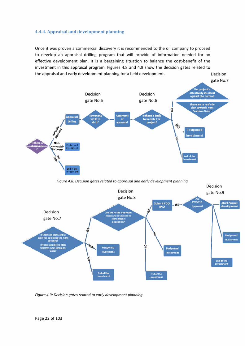
Once it was proven a commercial discovery it is recommended to the oil company to proceed to develop an appraisal drilling program that will provide of information needed for an effective development plan. It is a bargaining situation to balance the cost‐benefit of the investment in this appraisal program. Figures 4.8 and 4.9 show the decision gates related to the appraisal and early development planning for a field development.
Figure 4.8: Decision gates related to appraisal and early development planning.
Figure 4.9: Decision gates related to early development planning.
Decision gate No.5
Decision gate No.6
Decision gate No.7
Decision gate No.8
Decision gate No.7
Decision gate No.9
Page 23 of 103
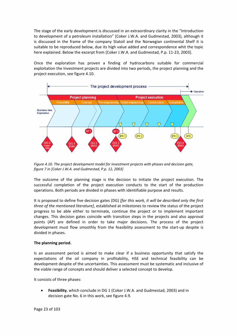
The stage of the early development is discussed in an extraordinary clarity in the “Introduction to development of a petroleum installation” (Coker J.W.A. and Gudmestad, 2003), although it is discussed in the frame of the company Statoil and the Norwegian continental Shelf it is suitable to be reproduced below, due its high value added and correspondence whit the topic here explained. Below the excerpt from [Coker J.W.A. and Gudmestad, P.p. 11‐23, 2003]. Once the exploration has proven a finding of hydrocarbons suitable for commercial exploitation the Investment projects are divided into two periods, the project planning and the project execution, see figure 4.10. Figure 4.10. The project development model for investment projects with phases and decision gate, figure 7 in [Coker J.W.A. and Gudmestad, P.p. 12, 2003] The outcome of the planning stage is the decision to initiate the project execution. The successful completion of the project execution conducts to the start of the production operations. Both periods are divided in phases with identifiable purpose and results.
It is proposed to define five decision gates (DG) [for this work, it will be described only the first three of the mentioned literature], established at milestones to review the status of the project progress to be able either to terminate, continue the project or to implement important changes. This decision gates coincide with transition steps in the projects and also approval points (AP) are defined in order to take major decisions. The process of the project development must flow smoothly from the feasibility assessment to the start‐up despite is divided in phases.
The planning period. Is an assessment period is aimed to make clear if a business opportunity that satisfy the expectations of the oil company in profitability, HSE and technical feasibility can be development despite of the uncertainties. This assessment must be systematic and inclusive of the viable range of concepts and should deliver a selected concept to develop. It consists of three phases:
• Feasibility, which conclude in DG 1 (Coker J.W.A. and Gudmestad, 2003) and in decision gate No. 6 in this work, see figure 4.9.
Page 24 of 103
• Concept, which conclude in DG 2 (Coker J.W.A. and Gudmestad, 2003) and in decision gate No. 7 in this work, see figure 4.9.
• Pre‐engineering, which conclude in DG 1 (Coker J.W.A. and Gudmestad, 2003) and in decision gate No. 8 in this work, see figure 4.9.
The main purpose of the feasibility phase is to establish and document whether a business opportunity or a hydrocarbon find is technically feasible and has an economic potential in accordance with the corporate business plan to justify further development. The feasibility phase is initiated at DG 0 with a project agreement that defines the task, goal, framework and budget. The feasibility phase leads to decision gate DG 1, “Decision to start concept development” (BoK). [Coker J.W.A. and Gudmestad, P.p. 12, 2003].
The purpose of the concept phase is to provide a firm definition of the design (resource and product) basis and to identify all relevant and feasible technical and commercial concepts. Further to evaluate and define the selected alternative (preferably one) and confirm that the profitability and feasibility of the business opportunity will be in accordance with the corporate requirements and business plans. The concept phase leads to the selection of the concept(s) (AP1) to be further developed up to decision gate DG 2, “Provisional project sanction” (BoV). [Coker J.W.A. and Gudmestad, P.p. 15, 2003]. The purpose of the pre‐engineering phase is to further develop and document the business opportunity based on the selected concept(s) to such a level that a final project sanction can be made, application to authorities can be sent and contracts can be entered into. The preengineering phase leads to approval point 2 (AP2), “Application to the authorities”, and to decision gate 3 (DG 3) “ Project sanction” (BoG). [Coker J.W.A. and Gudmestad, P.p. 19, 2003].
An additional point is the submission and approval of the plan of development and the plan of installation and operations. Coker and Gudmestad (2003) explain this point as Approval point 2, here corresponding to the Decision gate No. 9. See figure 4.9.
Approval point 2 (AP 2), "Application to the authorities" The project shall compile and prepare for submittal of the necessary application(s) for approval of the facility development in accordance with the relevant laws and regulations. It is particularly important to have undertaken an analysis to determine which requirements apply. For projects within the jurisdiction of the Norwegian Petroleum Act, a “Plan for development and operation” (PDO) (Norwegian: PUD) or a “Plan for installation and operation” (PIO) (Norwegian: PAD) is required. The PDO / PIO shall be prepared in accordance with the document “Guidelines for PDO and PIO”, issued by the Norwegian Petroleum Directorate. The PDO / PIO shall be approved by the responsible business unit, corporate management (KL), the board and the partners, before it is submitted. When the partnership submits a PDO / PIO to the authorities, this represents a commitment by the partnership to carry out the project development. For projects in this category, completion of the PDO / PIO and DG 3 (BoG) should occur at the same time. [Coker J.W.A. and Gudmestad, P.p. 21, 2003].
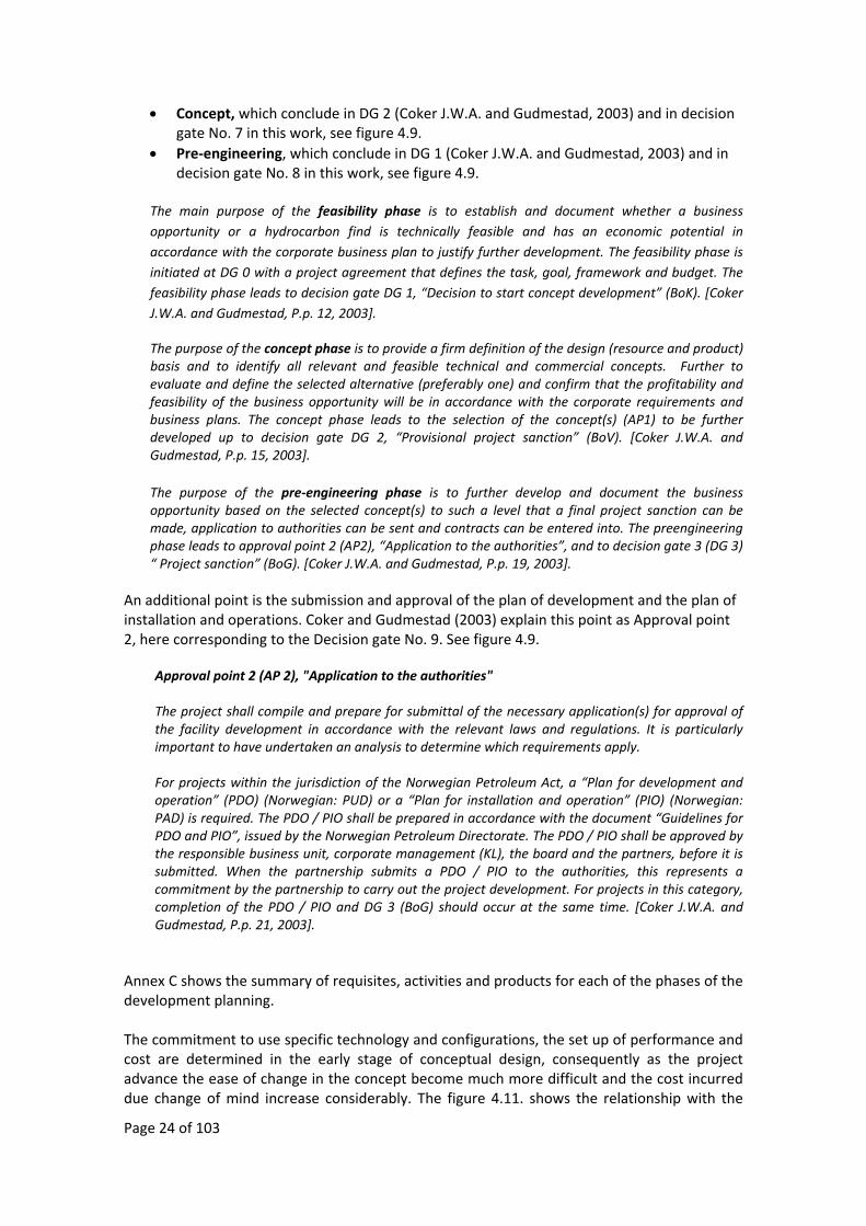
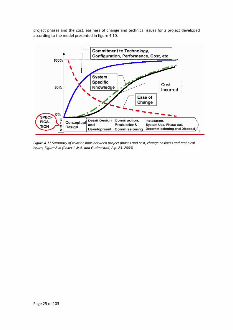
Annex C shows the summary of requisites, activities and products for each of the phases of the development planning. The commitment to use specific technology and configurations, the set up of performance and cost are determined in the early stage of conceptual design, consequently as the project advance the ease of change in the concept become much more difficult and the cost incurred due change of mind increase considerably. The figure 4.11. shows the relationship with the
Page 25 of 103
project phases and the cost, easiness of change and technical issues for a project developed according to the model presented in figure 4.10.
Figure 4.11 Summary of relationships between project phases and cost, change easiness and technical issues, Figure 8 in [Coker J.W.A. and Gudmestad, P.p. 23, 2003)
Page 26 of 103
5. Concept Selection and Life Cycle Cost
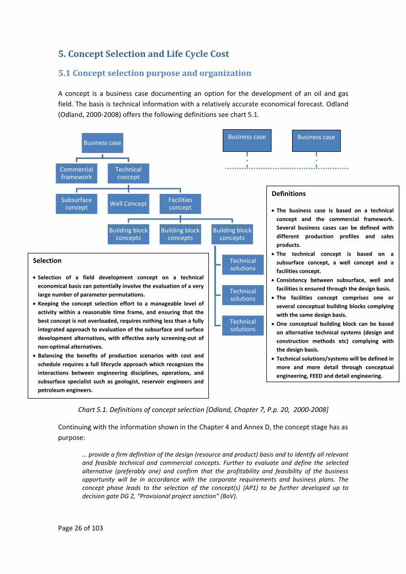
5.1 Concept selection purpose and organization A concept is a business case documenting an option for the development of an oil and gas field. The basis is technical information with a relatively accurate economical forecast. Odland (Odland, 2000‐2008) offers the following definitions see chart 5.1.
Chart 5.1. Definitions of concept selection [Odland, Chapter 7, P.p. 20, 2000‐2008]
Continuing with the information shown in the Chapter 4 and Annex D, the concept stage has as purpose:
… provide a firm definition of the design (resource and product) basis and to identify all relevant and feasible technical and commercial concepts. Further to evaluate and define the selected alternative (preferably one) and confirm that the profitability and feasibility of the business opportunity will be in accordance with the corporate requirements and business plans. The concept phase leads to the selection of the concept(s) (AP1) to be further developed up to decision gate DG 2, “Provisional project sanction” (BoV).
Definitions
• The business case is based on a technical concept and the commercial framework. Several business cases can be defined with different production profiles and sales products.
• The technical concept is based on a subsurface concept, a well concept and a facilities concept.
• Consistency between subsurface, well and facilities is ensured through the design basis.
• The facilities concept comprises one or several conceptual building blocks complying with the same design basis.
• One conceptual building block can be based on alternative technical systems (design and construction methods etc) complying with the design basis.
• Technical solutions/systems will be defined in more and more detail through conceptual engineering, FEED and detail engineering.
Selection
• Selection of a field development concept on a technical economical basis can potentially involve the evaluation of a very large number of parameter permutations.
• Keeping the concept selection effort to a manageable level of activity within a reasonable time frame, and ensuring that the best concept is not overloaded, requires nothing less than a fully integrated approach to evaluation of the subsurface and surface development alternatives, with effective early screening‐out of non‐optimal alternatives.
• Balancing the benefits of production scenarios with cost and schedule requires a full lifecycle approach which recognizes the interactions between engineering disciplines, operations, and subsurface specialist such as geologist, reservoir engineers and petroleum engineers.
Business case
Commercial framework
Technical concept
Subsurface concept Well Concept Facilities
concept
Building block concepts
Building block concepts
Building block concepts
Technical solutions
Technical solutions
Technical solutions
Business case Business case
Page 27 of 103
Different sources of literature, for example (Karsan, 2005) also relate the “Front End Loading (FEL)” processes, these are defined as all the activities that precede the start of the basic design phase and these should deliver:
• A well defined field development plan.
• Basis for conceptual design.
• Configuration of the field as well as conceptual drawings of major components of the development.
• Concept cost estimate +/‐ 40%.
Ignoring small differences it will be assumed that the concept stage is not different from the FEL, along this work and hence It will not be a differentiation of both terms hereby.
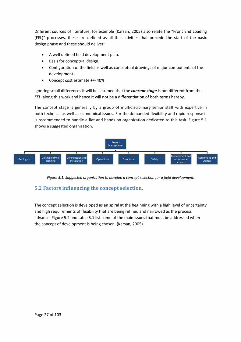
The concept stage is generally by a group of multidisciplinary senior staff with expertice in both technical as well as economical issues. For the demanded flexibility and rapid response it is recommended to handle a flat and hands on organization dedicated to this task. Figure 5.1 shows a suggested organization.
Figure 5.1. Suggested organization to develop a concept selection for a field development.
5.2 Factors influencing the concept selection.
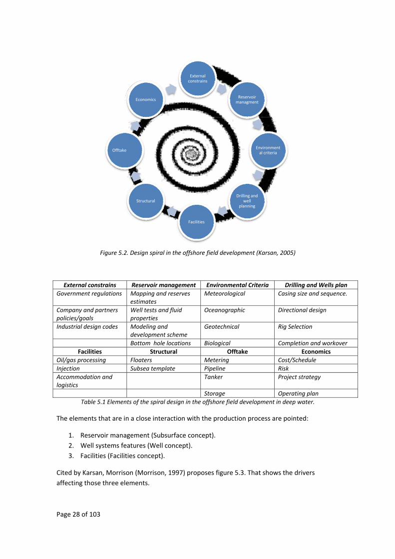
The concept selection is developed as an spiral at the beginning with a high level of uncertainty and high requirements of flexibility that are being refined and narrowed as the process advance. Figure 5.2 and table 5.1 list some of the main issues that must be addressed when the concept of development is being chosen. (Karsan, 2005).
Project Management
Geologists Drilling and wel planning
Construction and installation Operations Structural Safety
Procurement and economical analysis
Equipment and utilities
Page 28 of 103
Figure 5.2. Design spiral in the offshore field development (Karsan, 2005)
External constrains Reservoir management Environmental Criteria Drilling and Wells planGovernment regulations Mapping and reserves
estimates Meteorological Casing size and sequence.
Company and partners policies/goals
Well tests and fluid properties
Oceanographic Directional design
Industrial design codes Modeling and development scheme
Geotechnical Rig Selection
Bottom hole locations Biological Completion and workoverFacilities Structural Offtake Economics
Oil/gas processing Floaters Metering Cost/Schedule Injection Subsea template Pipeline Risk Accommodation and logistics
Tanker Project strategy
Storage Operating plan Table 5.1 Elements of the spiral design in the offshore field development in deep water.
The elements that are in a close interaction with the production process are pointed:
1. Reservoir management (Subsurface concept). 2. Well systems features (Well concept). 3. Facilities (Facilities concept).
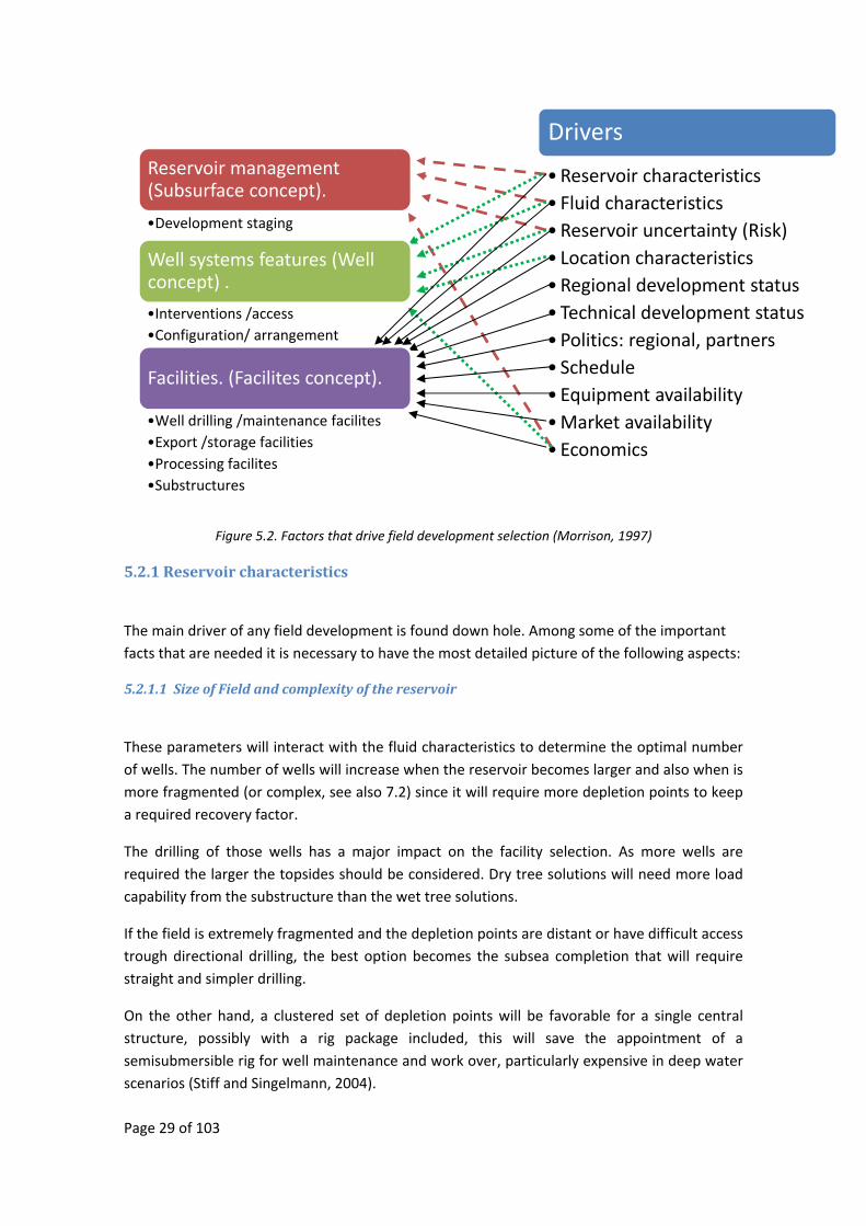
Cited by Karsan, Morrison (Morrison, 1997) proposes figure 5.3. That shows the drivers affecting those three elements.
External constrains
Reservoir managment
Environmental criteria
Drilling and well
planning
Facilities
Structural
Offtake
Economics
Page 29 of 103
Figure 5.2. Factors that drive field development selection (Morrison, 1997)
5.2.1 Reservoir characteristics
The main driver of any field development is found down hole. Among some of the important facts that are needed it is necessary to have the most detailed picture of the following aspects:
5.2.1.1 Size of Field and complexity of the reservoir
These parameters will interact with the fluid characteristics to determine the optimal number of wells. The number of wells will increase when the reservoir becomes larger and also when is more fragmented (or complex, see also 7.2) since it will require more depletion points to keep a required recovery factor.
The drilling of those wells has a major impact on the facility selection. As more wells are required the larger the topsides should be considered. Dry tree solutions will need more load capability from the substructure than the wet tree solutions.
If the field is extremely fragmented and the depletion points are distant or have difficult access trough directional drilling, the best option becomes the subsea completion that will require straight and simpler drilling.
On the other hand, a clustered set of depletion points will be favorable for a single central structure, possibly with a rig package included, this will save the appointment of a semisubmersible rig for well maintenance and work over, particularly expensive in deep water scenarios (Stiff and Singelmann, 2004).
Drivers
•Reservoir characteristics• Fluid characteristics•Reservoir uncertainty (Risk)• Location characteristics•Regional development status• Technical development status•Politics: regional, partners• Schedule• Equipment availability•Market availability• Economics
Reservoir management (Subsurface concept).
•Development staging
Well systems features (Well concept) .
•Interventions /access•Configuration/ arrangement
Facilities. (Facilites concept).
•Well drilling /maintenance facilites•Export /storage facilities•Processing facilites•Substructures
Page 30 of 103
Odland (Odland, 2000‐2008) also mentions that in case of larger fields it might be reasonable to think of the development as made up of several hub structures. More than one major structure in the field will open the possibility of increased recovery factor, more options for handling and transport of the hydrocarbons as well as risk and reliability robustness.
5.2.1.2. Expected Production Rate
As a result of a big and pressurized reservoir a high production rate can be foreseen. This will need more processing equipment leading to higher loads in the topsides. It will be necessary also larger export facilities. The concept will need consequently much more capacity for space and weight. The balance between produce at high rate or undersize the facilities must be assessed in this case. (Stiff and Singelmann, 2004)
5.2.1.3. Quantity of Gas and pressurization
A high pressure field with a relatively high content of gas leads to increasing need of processing equipment. Small fields might not be economical to exploit if the only solution is a large floating structure with capability to process the gas, in this case the subsea solutions become an attractive concept to study (Stiff and Singelmann, 2004).
Several options for handling of gas can be reviewed in the MMS study “Technology assessment of alternatives for handling associated gas produced from deepwater oil developments in the GOM” (Ward et. al., 2006).
5.2.1.4 Length of field life
Another aspect is the influence on the decommissioning considerations since some concepts such as SPAR’s, production semisubmersibles and FPSO’s can be reused when a field is exhausted. On the contrary, a TLP will represent a complex scenario for its relocation (Stiff and Singelmann, 2004).
Odland (Odland, 2000‐2008) also points out that in small field developments it might be an option for the operator companies to establish leasing agreements instead of commit to the construction of the production assets.
5.2.2. Fluid characteristics
5.2.2.1 Type of Crude
The subsea concepts are the best solution when it is anticipated that the wells will have low workover / interventions requirements and a high‐quality flow assurance (Dry gas reservoirs, free of parafins, etc.) The solution for complex flow assurance might involve the use of chemicals and other technologies, but they might be cost prohibitive (Stiff and Singelmann, 2004).
Page 31 of 103
5.2.2.2. Need for Workover and Intervention.
All the types of wells will eventually require some kind of maintenance; they can be from a simple intervention (for example a coil tubing operation) to full work over (recompletion) procedure to hit a different pay zone.
Nergaard (Nergaard, 2009) gives a definition of the two terms and explains their purposes as:
Workover: The term is used for a full overhaul of a well. It reflects the full capacity to change production equipment (tubing etc) in the well as well as the Xmas tree itself. This implies the use of a rig with fullbore BOP and marine riser. This means the we have to apply the same capacity systems as used during initial completion of the well. Full overhaul/workover might imply a full recompletion of the well. Using a full capacity drilling/completion rig offers the full capacity for redrilling, branch drilling and recompletion. In some cases we see the full capacity WOI system referred to as Category C intervention: heavy well intervention.
Well intervention: This term is used commonly for all vertical interventions that is done during the wells production life, i.e. after initial completion. The term is most commonly used for the lighter interventions; those implying that operations take place inside and through the Xmas tree and the tubing. These are:
Category B intervention: medium well intervention, with smaller bore riser.
Category A intervention: light well intervention – LWI, through water wireline operations.
The purpose of the interventions is to increase the recovery rate and also as required:
• Survey – mapping status‐data gathering. • Change status (ex open/close zones – smart wells) • Repair • Measures for production stimulation.
When the facility has a drilling package on board, or the capability to install one, the cost of these well interventions become lower than in the subsea developments, where for the same operations a dedicated type of vessel must be appointed (a semisubmersible with a day rate of 500,000 USD per day for example). Light intervention vessels are available at a lower rate but with lower capabilities (Stiff and Singelmann, 2004).
5.2.3. Reservoir uncertainty (Risk)
Although oil companies invest a lot of time and resources in the de risking of their investments (See 4.4.2) there is a substantial risk that might be the result of a limited appraisal of the discovery. The best option in this case is to have a flexible concept designed to be able to adapt to possible resizing of the production rate as well as ability to accommodate more wells or supplementary process capability. These options, of course, have a cost that must be evaluated.
Page 32 of 103
5.2.4. Location characteristics
5.2.4.1 Water Depth
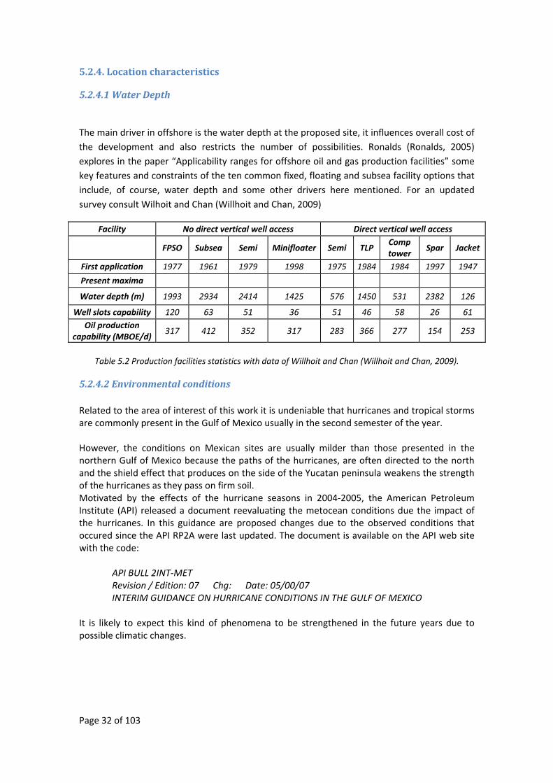
The main driver in offshore is the water depth at the proposed site, it influences overall cost of the development and also restricts the number of possibilities. Ronalds (Ronalds, 2005) explores in the paper “Applicability ranges for offshore oil and gas production facilities” some key features and constraints of the ten common fixed, floating and subsea facility options that include, of course, water depth and some other drivers here mentioned. For an updated survey consult Wilhoit and Chan (Willhoit and Chan, 2009)
Facility No direct vertical well access Direct vertical well access
FPSO Subsea Semi Minifloater Semi TLP Comp tower
Spar Jacket
First application 1977 1961 1979 1998 1975 1984 1984 1997 1947
Present maxima
Water depth (m) 1993 2934 2414 1425 576 1450 531 2382 126
Well slots capability 120 63 51 36 51 46 58 26 61 Oil production
capability (MBOE/d) 317 412 352 317 283 366 277 154 253
Table 5.2 Production facilities statistics with data of Willhoit and Chan (Willhoit and Chan, 2009).
5.2.4.2 Environmental conditions Related to the area of interest of this work it is undeniable that hurricanes and tropical storms are commonly present in the Gulf of Mexico usually in the second semester of the year. However, the conditions on Mexican sites are usually milder than those presented in the northern Gulf of Mexico because the paths of the hurricanes, are often directed to the north and the shield effect that produces on the side of the Yucatan peninsula weakens the strength of the hurricanes as they pass on firm soil. Motivated by the effects of the hurricane seasons in 2004‐2005, the American Petroleum Institute (API) released a document reevaluating the metocean conditions due the impact of the hurricanes. In this guidance are proposed changes due to the observed conditions that occured since the API RP2A were last updated. The document is available on the API web site with the code:
API BULL 2INT‐MET Revision / Edition: 07 Chg: Date: 05/00/07
INTERIM GUIDANCE ON HURRICANE CONDITIONS IN THE GULF OF MEXICO
It is likely to expect this kind of phenomena to be strengthened in the future years due to possible climatic changes.

Page 33 of 103
5.2.4.3. Geotechnical conditions
A careful study is needed for the installation and decommissioning, a soft soil could be as risky as an extreme tropical storm and the combined effects might be catastrophic.
5.2.5 Regional development status
In a region like U.S. Gulf of Mexico an enhanced possibility to develop small fields exists, due its extensive networks of pipelines. The distance to the facilities is a major restrictive element to consider for small to medium field developments because of flow assurance issues; due to this reason a major content of gas in the production fluids has a longer reach to be exported.
The development of hub´s in any case might create the feasibility for further developments in an area. Even in the case of ownership of different companies it is possible to establish agreements to allow the transportation of crude per a transfer fee (Stiff and Singelmann, 2004).
5.2.6. Technical development status.
Sometimes the companies face options to develop fields by using new technologies. However, operator companies, either national or international usually prefer a conservative approach to the development and use of new technologies. This adversity change when the technology become proven, but still it would be necessary to implement effective programs for technology acquisition.
5.2.7 Politics
The governmental, corporative and industrial polices usually have the same weight as the technical and economical considerations. The governments may ask for the fulfillment of tariffs of local contents, restrictions on particular development options, health, safety and environment regulations, and even recovery factors like the NPD in Norway, see 7.2.
Corporate politics will be evident in the selection of specific development options because of the perception to have lower risk than others based on previous experiences of the operator. Also for the preference of contractors companies that are viewed as more reliable, even though those companies can offer just a limited pool of options where the best concept is not necessarily included (Stiff and Singelmann, 2004).
5.2.8. Schedule
The drilling strategy might have a powerful impact on the schedule to get the first oil. A company might save a lot of time running a partial or total pre‐drilling program while they are constructing the floating structures and/or the subsea systems. Pre drilling in deep water means the appointment of semisubmersibles or drilling ships that will represent a considerable
Page 34 of 103
cost against the option of some floaters that might have the possibility to drill from the same structure. This drilling strategy of course is part of the decisions that must be analyzed in the conceptual stage.
5.2.9. Equipment availability
The heavy lift vessels are examples of scarce but unavoidable tools for some concept of field development. Hence the appointment of them become a fact of major importance when the concept is defined.
5.2.10. Market availability
The gas is the most representative example of one product that must have a mature market to make it feasible to commit a field development. In contrast to the oil that might be stabilized and transported by tankers to the market, the gas production needs to be delivered at a constant basis to a market because the storage cost of large amounts of product is extremely costly if technically feasible.
5.2.11. Economics
Practically in all the past examples the economics is part of the debate between one options or another.
5.3 Life Cycle Cost in concept selection processes
The economical analysis for field development are essentially Life cycle cost analysis, the minimum requirements are already suggested initially for the oil and gas industry by the Norwegian Standards (Norsok).
• O‐CR‐002 Life cycle cost for production facility (Rev. 1, April 1996)
• O‐CR‐001 Life cycle cost for systems and equipment (Rev. 1, April 1996)
Those standards were withdrawn in 2001 when the series ISO 15663 were published:
• ISO 15663‐1:2000 Petroleum and natural gas industries ‐‐ Life cycle costing ‐‐ Part 1: Methodology.
• ISO 15663‐2:2001 Petroleum and natural gas industries ‐‐ Life‐cycle costing ‐‐ Part 2: Guidance on application of methodology and calculation methods.
• ISO 15663‐3:2001 Petroleum and natural gas industries ‐‐ Life‐cycle costing ‐‐ Part 3: Implementation guidelines.
The use of the LCC in most of the concept studies is limited to the Capital Expenditures (CAPEX) and Operational Expenditures (OPEX). Goldsmith (Goldsmith et. al., 2000) propose a much more ample spectra to calculate LCC including the risk and the reliability costs associated with
Page 35 of 103
the field development options. Below the methodology proposed by Goldsmith to estimate the lifecycle cost of subsea production systems [Goldsmith et. al., Sections 2.1‐2.3.3, 2000].
2.1 Introduction
The economics of deepwater developments are different from shelf activities. Deepwater is characterized by high capital expenditures with relatively low operational expenditures and high sustainable production rates ‐ hence high costs for production interruption.
Field development profitability is a function of many income and expense factors such as capital expenditures (CAPEX), operating expenditures (OPEX), production rate, product price and the frequency of completion component failures. Component failures reduce the field total production rate and increase intervention expenditures.
Until recently it was quite common for the decision making process used to evaluate deepwater ventures to focus on optimizing the balance between potential revenue, CAPEX and OPEX according to the equation:
Profit = Max (Revenue ‐ CAPEX ‐ OPEX) (2.1)
The shortcoming in this equation is that it does not take into account unscheduled and unplanned events that have the potential to destroy a facility, tarnish a company’s reputation, pollute the environment, and/or shut down production for a long time. Major accidents, although highly unlikely, have the potential to put a facility out of business for 3, 6, 12 months or even render it totally useless.
When moving into deeper water, the economic penalty for delayed/lost production becomes greater. The uncertainty related to whether “unforeseen” events will occur is also increased as prototype and novel technology are introduced into an operating environment not encountered in shallow water platform design. Furthermore, subsea well system repairs and interventions also become more expensive and are associated with longer delays due to reduced availability and increased mobilization times for the required repair vessels. The alternative to a subsea system, a dry tree tieback concept provides the efficiency and the convenience of direct well access, but requires the surface host to support the weight of permanently attached production/intervention risers for which the load cost penalty and the likelihood of a riser leak increases with water depth.
The implications of disasters and business interruptions should be incorporated into business decision analyses that seek to evaluate the viability of alternative designs. These analyses introduce two more components to the economic “balance”, namely, risk expenditures (RISKEX1) and reliability/availability/maintainability expenditures (RAMEX2). It takes a balanced, mature appraisal of the uncertainties and risks involved when considering front‐end cost savings (CAPEX) that may have detrimental consequences on initial, intermediate and long‐term revenue streams.
Inclusion of an "unforeseen" RISKEX and RAMEX element into equation (2.1) modifies the economic model to:
1 RISK Expenditures (RISKEX) are defined as the costs associated with the risks of a blowout. It is derived by estimating the frequency of the event and multiplying the frequency by the estimated cost (clean‐up cost, outrage cost, asset damage cost and business interruption cost) for that event. 2 Reliability/Availability/Maintainability Expenditures (RAMEX) are defined as the cost associated with lost revenues and interventions due to component failures.
Page 36 of 103
Profit = Max (Revenue ‐ CAPEX ‐ OPEX – RISKEX ‐ RAMEX) (2.2)
The methodology is developed to permit predictions of lifetime cost for a field development based on statistical and judgmental reliability data and assumed system parameters. It might be asked “Why not simply estimate the lifetime cost for a field development rather than estimating all these input parameters?” The answers are:
• The system is broken down to a level where some experience data is available and where it is possible to evaluate failure modes and their corresponding effect on system level.
• The quality of the input data (reliability of completion string components, sand control system failures, subsea equipment, risers, individual well production profiles, rig availability time, rig spread costs, etc.) is independently evaluated to minimize bias.
• The methodology and spreadsheet tool “model” show the sensitivity to changes in specific input data that is not readily apparent otherwise.
• This model is especially useful to determine which parameters most influence field development cost. The quality of data for these parameters can then be scrutinized to achieve the maximum practical quality. Likewise, time is not wasted by attempting to improve the quality of data that are of minor importance.
• Sensitivity analyses can determine the financial incentive for improving reliabilities of components.
2.2 System Boundaries
The systems that can be analyzed by using the proposed methodology are typical highrate, deepwater well completion systems and cover both subsea well tieback and dry tree tieback concepts. A subsea well intervention has longer rig availability and mobilization time, is more sensitive to weather conditions, and is associated with higher day rates for the repair resource. However, all these parameters are part of the input data specified by the user.
The methodology includes:
Subsea: Downhole completion components, casing, wellhead equipment, subsea production trees, flowline jumpers, tie‐in sleds, flowlines and risers (up to the boarding valve), subsea control module, control jumpers, subsea distribution units, umbilical termination assemblies, umbilicals, topside controls and chemical injection points.
Dry Tree: Downhole completion components, casing, wellhead equipment, risers, tensioners/air cans, surface production tree and manifold up to the 1st stage separation isolation valve.
For both concepts the well intervention equipment (risers, BOPs, controls, etc.) necessary to install and workover the completion equipment are included.
Examples of sand control systems considered by this project are frac‐packs and horizontal laterals with gravel pack.
2.3 Life Cycle Cost Calculations
The CAPEX, OPEX and RISKEX occur during different times in the field‐life. The net present value of future costs is used to take the time value of money into account. The lifecycle cost is calculated by:
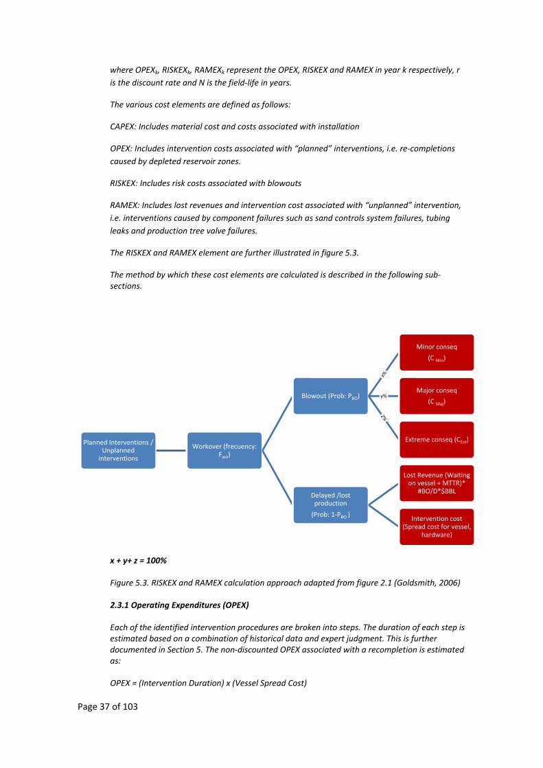
Page 37 of 103
where OPEXk, RISKEXk, RAMEXk represent the OPEX, RISKEX and RAMEX in year k respectively, r is the discount rate and N is the field‐life in years.
The various cost elements are defined as follows:
CAPEX: Includes material cost and costs associated with installation
OPEX: Includes intervention costs associated with “planned” interventions, i.e. re‐completions caused by depleted reservoir zones.
RISKEX: Includes risk costs associated with blowouts
RAMEX: Includes lost revenues and intervention cost associated with “unplanned” intervention, i.e. interventions caused by component failures such as sand controls system failures, tubing leaks and production tree valve failures.
The RISKEX and RAMEX element are further illustrated in figure 5.3.
The method by which these cost elements are calculated is described in the following sub‐sections.
x + y+ z = 100% Figure 5.3. RISKEX and RAMEX calculation approach adapted from figure 2.1 (Goldsmith, 2006) 2.3.1 Operating Expenditures (OPEX) Each of the identified intervention procedures are broken into steps. The duration of each step is estimated based on a combination of historical data and expert judgment. This is further documented in Section 5. The non‐discounted OPEX associated with a recompletion is estimated as: OPEX = (Intervention Duration) x (Vessel Spread Cost)
Planned Interventions / Unplanned interventions
Workover (frecuency: Fwo)
Blowout (Prob: PBO)
Minor conseq
(C Min)
y%Major conseq
(C Maj)
Extreme conseq (CExt)
Delayed /lost production
(Prob: 1‐PBO )
Lost Revenue (Waiting on vessel + MTTR)*
#BO/D*$BBL
Intervention cost (Spread cost for vessel,
hardware)
Page 38 of 103
2.3.2 Risk Expenditures (RISKEX) The probability of failure of the well completion system is a function of the probability of failure during the various operating modes (drilling, completion, normal production, workovers and re‐completions). The lifetime probability of a blowout is calculated as:
P(BO during lifetime) = P(drilling)+ P(initial compl.)+ P(prod) + ∑ ) +∑ . )
The cost of a blowout depends on the size of the release (“Limited, “Major” or “Extreme”). The Risk Cost (RC) associated with a certain activity (j) was calculated as:
RC(j)= ∑ ) i {limited, major, extreme}
where Probi(activity j) is the probability of a blowout of size i during activity j, and Ci is the cost of leak of size, i {limited, major, extreme}. This is further described in Section 7. 2.3.3 Reliability, Availability and Maintainability Expenditures (RAMEX) The RAMEX is divided into two: • Cost associated with lost revenues • Cost associated with interventions For the model developed, the consequence for the production in a given year depends on the following: • The production rate at the time the failure occurred • Lost capacity while waiting on repair resources • Availability time for the repair resources • Mobilization time for the repair resources • Active repair time An example is given below: Example 1: • Failure: Workover (WO) required to repair the failure in year • Resource: Rig • Production loss: 50% while waiting on rig (90 days) + 30 days for WO. • Production rate: 10,000 BOPD in year 3. • Lost volume: The financial consequence of a well failure will in addition to the factors discussed above depend on: • Failure time • Oil operating margin in year produced ($/BBL) • Spread cost for intervention vessel ($/day) An example is given below: Example 2: • WO required to repair the failure • Resource: Rig • Failure time: year 3 • Production loss: 50% while waiting on rig (90 days) + 30 days for WO

Page 39 of 103
• Production rate: 10,000 BOPD in year 3 • Spread cost for Rig: $100,000 per day • Oil operating margin in year produced: $10/BBL • Discount rate: 15% • Financial Consequence (FC): FC = Lost Revenues + Intervention Cost FC = 0.5* 90days 1* 30days)* 10,000BOPD*($10 per BO/(1+0.15)3)+ ($100,000/d * 30days)/ (1 0.15) ≈ 4.9MM + 2MM = 6.9MM
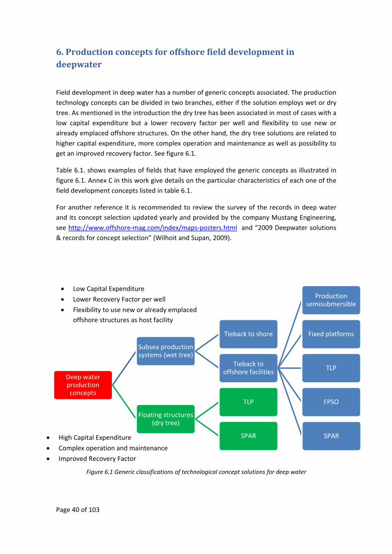
Page 40 of 103
6. Production concepts for offshore field development in deepwater
Field development in deep water has a number of generic concepts associated. The production technology concepts can be divided in two branches, either if the solution employs wet or dry tree. As mentioned in the introduction the dry tree has been associated in most of cases with a low capital expenditure but a lower recovery factor per well and flexibility to use new or already emplaced offshore structures. On the other hand, the dry tree solutions are related to higher capital expenditure, more complex operation and maintenance as well as possibility to get an improved recovery factor. See figure 6.1.
Table 6.1. shows examples of fields that have employed the generic concepts as illustrated in figure 6.1. Annex C in this work give details on the particular characteristics of each one of the field development concepts listed in table 6.1.
For another reference it is recommended to review the survey of the records in deep water and its concept selection updated yearly and provided by the company Mustang Engineering, see http://www.offshore‐mag.com/index/maps‐posters.html and “2009 Deepwater solutions & records for concept selection” (Wilhoit and Supan, 2009).
Figure 6.1 Generic classifications of technological concept solutions for deep water
Deep water production concepts
Subsea production systems (wet tree)
Tieback to shore
Tieback to offshore facilities
Production semisubmersible
Fixed platforms
TLP
FPSO
SPAR
Floating structures (dry tree)
TLP
SPAR
• Low Capital Expenditure
• Lower Recovery Factor per well
• Flexibility to use new or already emplaced offshore structures as host facility
• High Capital Expenditure
• Complex operation and maintenance
• Improved Recovery Factor
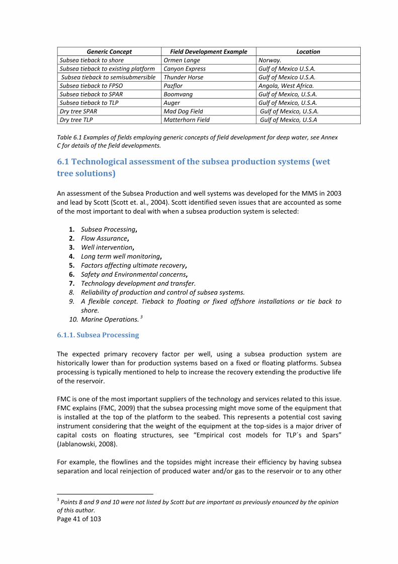
Page 41 of 103
Generic Concept Field Development Example Location Subsea tieback to shore Ormen Lange Norway. Subsea tieback to existing platform Canyon Express Gulf of Mexico U.S.A. Subsea tieback to semisubmersible Thunder Horse Gulf of Mexico U.S.A. Subsea tieback to FPSO Pazflor Angola, West Africa. Subsea tieback to SPAR Boomvang Gulf of Mexico, U.S.A. Subsea tieback to TLP Auger Gulf of Mexico, U.S.A. Dry tree SPAR Mad Dog Field Gulf of Mexico, U.S.A. Dry tree TLP Matterhorn Field Gulf of Mexico, U.S.A Table 6.1 Examples of fields employing generic concepts of field development for deep water, see Annex C for details of the field developments.
6.1 Technological assessment of the subsea production systems (wet tree solutions) An assessment of the Subsea Production and well systems was developed for the MMS in 2003 and lead by Scott (Scott et. al., 2004). Scott identified seven issues that are accounted as some of the most important to deal with when a subsea production system is selected:
1. Subsea Processing, 2. Flow Assurance, 3. Well intervention, 4. Long term well monitoring, 5. Factors affecting ultimate recovery, 6. Safety and Environmental concerns, 7. Technology development and transfer. 8. Reliability of production and control of subsea systems. 9. A flexible concept. Tieback to floating or fixed offshore installations or tie back to
shore. 10. Marine Operations. 3
6.1.1. Subsea Processing The expected primary recovery factor per well, using a subsea production system are historically lower than for production systems based on a fixed or floating platforms. Subsea processing is typically mentioned to help to increase the recovery extending the productive life of the reservoir. FMC is one of the most important suppliers of the technology and services related to this issue. FMC explains (FMC, 2009) that the subsea processing might move some of the equipment that is installed at the top of the platform to the seabed. This represents a potential cost saving instrument considering that the weight of the equipment at the top‐sides is a major driver of capital costs on floating structures, see “Empirical cost models for TLP´s and Spars” (Jablanowski, 2008). For example, the flowlines and the topsides might increase their efficiency by having subsea separation and local reinjection of produced water and/or gas to the reservoir or to any other
3 Points 8 and 9 and 10 were not listed by Scott but are important as previously enounced by the opinion of this author.
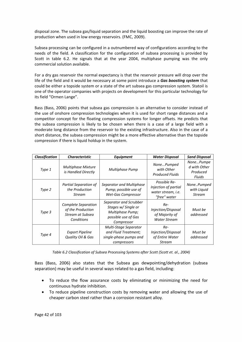
Page 42 of 103
disposal zone. The subsea gas/liquid separation and the liquid boosting can improve the rate of production when used in low energy reservoirs. (FMC, 2009). Subsea processing can be configured in a outnumbered way of configurations according to the needs of the field. A classification for the configuration of subsea processing is provided by Scott in table 6.2. He signals that at the year 2004, multiphase pumping was the only commercial solution available. For a dry gas reservoir the normal expectancy is that the reservoir pressure will drop over the life of the field and it would be necessary at some point introduce a Gas boosting system that could be either a topside system or a state of the art subsea gas compression system. Statoil is one of the operator companies with projects on development for this particular technology for its field “Ormen Lange”. Bass (Bass, 2006) points that subsea gas compression is an alternative to consider instead of the use of onshore compression technologies when it is used for short range distances and a competitor concept for the floating compression systems for longer offsets. He predicts that the subsea compression is likely to be chosen when there is a case of a large field with a moderate long distance from the reservoir to the existing infrastructure. Also in the case of a short distance, the subsea compression might be a more effective alternative than the topside compression if there is liquid holdup in the system. Classification Characteristic Equipment Water Disposal Sand Disposal
Type 1 Multiphase Mixture is Handled Directly
Multiphase Pump None...Pumped with Other
Produced Fluids
None…Pumped with Other Produced Fluids
Type 2 Partial Separation of
the Production Stream
Separator and Multiphase Pump; possible use of Wet‐Gas Compressor
Possible Re‐Injection of partial water stream, i.e.
"free" water
None..Pumped with Liquid Stream
Type 3
Complete Separation of the Production Stream at Subsea
Conditions
Separator and Scrubber Stages w/ Single or Multiphase Pump; possible use of Gas
Compressor
Re‐Injection/Disposal of Majority of Water Stream
Must be addressed
Type 4 Export Pipeline Quality Oil & Gas
Multi‐Stage Separator and Fluid Treatment;
single‐phase pumps and compressors
Re‐Injection/Disposal of Entire Water
Stream
Must be addressed
Table 6.2 Classification of Subsea Processing Systems after Scott (Scott et. al., 2004)
Bass (Bass, 2006) also states that the Subsea gas dewpointing/dehydration (subsea separation) may be useful in several ways related to a gas field, including:
• To reduce the flow assurance costs by eliminating or minimizing the need for continuous hydrate inhibition.
• To reduce pipeline construction costs by removing water and allowing the use of cheaper carbon steel rather than a corrosion resistant alloy.
Page 43 of 103
• To process close to sales quality or even reach sales quality that also addresses flow assurance needs.
6.1.2 Flow Assurance Scott (Scott et. al., 2004) refers that flow assurance is the term related to the study of the complex phenomena involving the transportation of produced fluids trough the producing and transportation flow lines. The produced fluids are a combination of hydrocarbon gases, crude oil/condensate and water together with hydrocarbon solids such as, hydrates, scale, wax, paraffin, asfaltenes, and other solids and gases such as sand, CO2, H2S. In order to get satisfactory recoveries rates it is necessary to identify the potential and quantify the magnitude of the produced fluid to be managed in the system. The flexibility of the system is required because different parameters of the produced fluid (pressures, temperatures, production fractions) involved in the design of the system are expected to change along the life of the project, and also that mentioned flexibility will be necessary to control during the transient periods of production (shutdown and restart). The design of a flow assurance program for a field needs to consider the requirements for all parts of the system for the entire production life. Some of those considerations are, production profiles, chemical injection & storage, produced fluids properties, host facility (pigging, fluid storage, tubulars (tubing & flowline ID’s) & handling, intervention capability, Insulation (tubing, wellhead, etc.), capital and operating costs.
Flow assurance also depends to a large extent if the development is for an oil or a gas reservoir. Flow assurance is much more challenging in oil than in gas producers, both of them will have corrosion and hydrate issues but in oil’s the wax, asphaltenes, scale and emulsion expectations should also be considered in the design. The gas systems can be managed with a flow assurance strategy driven by the injection of hydrate inhibitors chemicals such as MEG (monoethylene glycol), thermal isolation is usually not as demanding as in oil production but is an important factor in low temperature environments for example in the developments on the Norwegian continental shelf (Ball, 2006).
6.1.3. Well Intervention The cost of well interventions in subsea production systems is considerable higher compared to fixed or floating platforms with work over systems since they require the mobilization of MODU’s (Mobil offshore drilling units) or drilling ships for each well location. This issue is the main reason to select pressure boosting at the seafloor rather than artificial lift in the wellbore and has also motivated the development of Intelligent Well Technology (IWT) to increase the operative flexibility as an alternative to well intervention (Scott et. al., 2004).
Page 44 of 103
6.1.4. Long term well monitoring Scott (Scott et. al., 2004) refers to this long term well monitoring as Intelligent Well Technology (IWT), which compresses two main concepts: 1. Monitoring of measurements of down hole flow and/or reservoir conditions. The
measurement is performed by electronic devices or fiber optics, parameters currently functional today are pressure, temperature and flow rate.
2. Remotely control zones through on/off control or choking. The control is achieved by electric, hydraulic or electro‐hydraulic (hybrid) actuation of a valve or sleeve. Commercially available.
Control and monitoring are being accepted slowly due to concerns about complexity, reliability and cost. It does not matter how sophisticated is the installation when the system fails and workover is required. An additional motivation for further development of IWT in the Gulf of Mexico is that in this region there has been registered a large occurrence of Sustained Casing Pressure (SCP) in producing wells. Citing Wojtanowicz (Wojtanowicz et. al., 2001) “The Minerals Management Service (MMS) defines SCP as a pressure measurable at the casinghead of a casing annulus that rebuilds when bled down and that is not due solely to temperature fluctuations and is not a pressure that has been deliberately applied.”(Wojtanowicz et. al, P.p. 4, 2001). SCP is identified as a cause of leakages that are dangerous for personnel near well heads located on topsides of platforms and for the environment in subsea facilities. Currently is not possible for a monitor to access the outer with a subsea wellhead a necessary improvement is to find a way to develop the ability to monitor and remediate SCP.
6.1.5. Factors affecting ultimate recovery Scott (Scott et. al., 2004) also found that the multiphase flowlines that make possible the development of long subsea tiebacks reduce the ultimate recoveries. According to his work since the subsea wells operate with a continual high backpressure the energy that could be used to deplete more efficiently the reservoir is lost in the flow line and in the choke valves of the system.
6.1.6. Risk, safety and environmental concerns Although each facility is different due its design, functions and operation conditions, the remoteness of the subsea systems location reduces the risks to the personnel but still, the environment risks remain for subsea production systems. It is recommended to be as strict as reasonably possible with the safety system requirements defined for subsea production systems. (Brandt, 2004).
6.1.7. Technology development and transfer. As mentioned before, just some of the conceptually developed subsea production systems have been implemented commercially. Operator companies either national or international usually prefer a more conservative approach on the development of new technologies. This,
Page 45 of 103
however, is going to change when the technology become proven, but the implementation of effective programs of technology acquisition will still be necessary.
6.1.8. Reliability of production and control of subsea systems To obtain cost effective and reliable production and control systems are also challenges of major importance, this aspect is managed in general by redundancy in design and applying reliability centered design and maintenance philosophies. The reliability also implies a lot of work on the organization of the operators and contracting companies that are part of the subsea projects. The high amount of uncertainty due to restrictions in time and budgeting are a cause of increased risk in the design, construction, installation and operation of the systems. On the knowledge of the importance of human and organizational factors, API has released recently a “Recommended Practice for Subsea Production System Reliability and Technical Risk Management” API 17 N (API, 2009) This document has as purpose that the users of that RP gain a better understanding of how to manage an appropriate level of reliability throughout the life cycle of their subsea projects. The whole industry demand that the developers of subsea systems:
— recognize the trade off between up front reliability and engineering effort vs. operational maintenance effort, — provide better assurance of future performance of subsea systems, — effectively manage the risks from using novel equipment and standard equipment in novel applications, — schedule projects with sufficient time to address all the technical risks. [API, P.p. 1, 2009]
On the other hand, Scott (Scott et. al., 2004) mention in their work that most of the designs have focused on increasing component reliability and extending the mean time to failure to address intervention concerns. Remarkably the redundant systems were not found to be in widespread use due to the increased capital costs these systems incurred.
6.1.9. A flexible concept. Tieback to floating or fixed offshore installations or tie back to shore. The main benefit of the subsea production systems is that they are recognized to diminish the capital cost of the new developments since the construction expenditures of an entire new‐brand offshore platform are avoided. The subsea production systems might be quite different in form and size (ISO‐13628‐1,2005), they can be designed as:
• A single satellite well with a flowline linked to offshore platforms, floating or onshore processing facilities.
• Several wells located in one or more templates. • Wells or set of wells in templates clustered around a manifold with or without subsea
processing connected to facilities onshore or offshore.
Page 46 of 103
The concept of a subsea production system to shore has been used already in several developments around the world i.e. Snøhvit, Ormen Lange, Patricia Baleen, BHPBP Minerva, and ONGC G‐1. As example of deep water tiebacks to fixed platforms just as example is possible to mention, the Devils Creek, Pompano, Bullwinkle and Canyon Express, all of them located in U.S. Gulf of Mexico and acting as a host for subsea tiebacks. The subsea production systems are most often selection when a semisubmersible or a FPSO is employed, however there are recent developments that have used topside trees using a semisubmersible this are related to mild environment as West Africa. (Often, 2000). Odland summarizes the characteristics of the semisubmersible production units (Odland, 2008):
• Large number of risers, these facilities can handle a large number of slots for production and injection risers what made them suitable for larges and multifield tie back field developments.
• Good motion characteristics, due its proven dynamic characteristic response it is possible to have a high pay load on its top sides.
• New built or conversion, it is possible to use drilling rig hulls that are still usable and otherwise would face decommissioning.
• Not offer storage capability. • Have a spread mooring systems.
Lim and Ronalds (Lim and Ronalds, 2000) presented an historical and prospective review on the Semi submersible production systems and FPSO’s. In their view the floating production systems were developed initially (1970’s) for their advantages in deep water and reservoirs of short production life, at the beginning the semisubmersibles were common selected against FPSO’s because the concept offered:
• Drilling and workover capability for wells located just below the semi. • Good motion response (stability). • Availability of drilling rigs for conversion to production semis. • It was possible to use rigid risers before the technology of flexible risers appeared.
Later, at the end of 1980s and beginning of 1990 the semisubmersibles were recognized for their capabilities to operate in the deep water. At the beginning of the 2000’s the FPSO are more numerous than the semisubmersibles, some reasons for this are:
• Advantages of the shape of the hull of the FPSO’s, more stability and maniobrability. • Improvements in turret technology. • Preferable when used for small and remote oil fields.
The production semisubmersibles are also popular in case of gas reservoirs and compete with the new designs of SPAR’s and TLP’s when there is a large reservoir to exploit and a suitable
Page 47 of 103
infrastructure of pipelines is available. Its evolution has been remarkable, through developing new types of risers, hulls forms and methods of construction. Odland (Odland, 2008) also states that in deep water the principal challenge of the semisubmersible is related to the hydrodynamic effects that induce loss of position and slamming over the structure and the riser systems. A related issue with the deep water is its weight gain due both the mooring and the riser systems.
6.1.10 Marine operations. Regarding marine technology and operations, although important is not considered to be a challenge for the subsea production systems. After its installation the subsea facilities are considerable less exposed to environmental loads than the fixed and floating offshore units. However as stated in the Standard ISO ISO‐13628‐1:2005 “All applicable loads that can affect the subsea production system during all relevant phases, such as fabrication, storing, testing, transportation, installation, drilling/completion, operation and removal, should be defined and form the basis for the design” [ISO‐13628‐1,2005]. Since marine operations represent an important part of the costs of installation a summary of marine operations for both, subsea production systems as well as floating structures, is presented in Annex D.
6.2 Technological assessment of floating structures (dry tree solutions)
Any floating structure has as a purpose to extend the range of operation offshore by the provision of space to locate machinery and supplies for the exploitationn of oil and gas fields. The technical solutions are not so different from the ones that are installed onshore but the reduced weight and space capability is a major restriction for the equipment.
This topic is extensive and it is suggested for the reader to consider as a reference the ISO standard IS0 19904‐1, Floating offshore structures Part 1: Monohulls, semi‐submersibles and spars (ISO, 2006) which have been developed for this topic.
ISO 19904‐1:2006 provides requirements and guidance for the structural design and/or assessment of floating offshore platforms used by the petroleum and natural gas industries to support production, storage and/or offloading, drilling and production, production, storage and offloading, and drilling, production, storage and offloading. [ISO, Abstract, 2006]
Whilst the ISO standard IS0 19904‐2, Floating offshore structures Part 2: Tension Leg Platform is still in discussion and development process, “API RP 2T‐ Recommended Practice for Planning, Designing, and Constructing Tension Leg Platforms” is the suggested reference to know more about TLP´s.
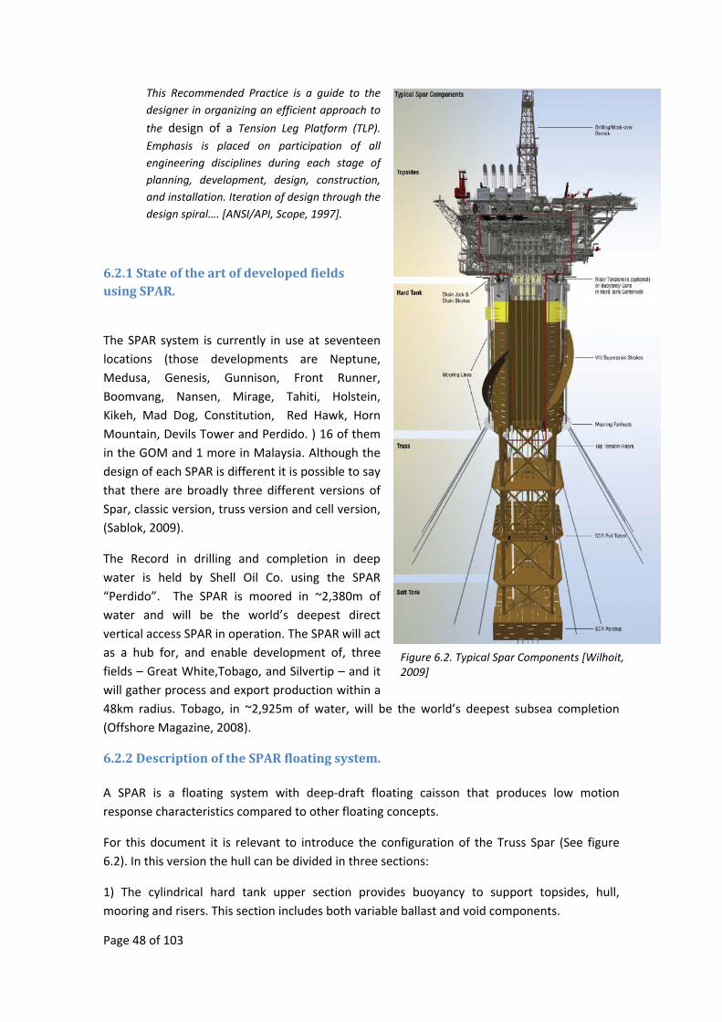
Page 48 of 103
This Recommended Practice is a guide to the designer in organizing an efficient approach to
the design of a Tension Leg Platform (TLP).
Emphasis is placed on participation of all engineering disciplines during each stage of planning, development, design, construction, and installation. Iteration of design through the design spiral…. [ANSI/API, Scope, 1997].
6.2.1 State of the art of developed fields using SPAR.
The SPAR system is currently in use at seventeen locations (those developments are Neptune, Medusa, Genesis, Gunnison, Front Runner, Boomvang, Nansen, Mirage, Tahiti, Holstein, Kikeh, Mad Dog, Constitution, Red Hawk, Horn Mountain, Devils Tower and Perdido. ) 16 of them in the GOM and 1 more in Malaysia. Although the design of each SPAR is different it is possible to say that there are broadly three different versions of Spar, classic version, truss version and cell version, (Sablok, 2009).
The Record in drilling and completion in deep water is held by Shell Oil Co. using the SPAR “Perdido”. The SPAR is moored in ~2,380m of water and will be the world’s deepest direct vertical access SPAR in operation. The SPAR will act as a hub for, and enable development of, three fields – Great White,Tobago, and Silvertip – and it will gather process and export production within a 48km radius. Tobago, in ~2,925m of water, will be the world’s deepest subsea completion (Offshore Magazine, 2008).
6.2.2 Description of the SPAR floating system. A SPAR is a floating system with deep‐draft floating caisson that produces low motion response characteristics compared to other floating concepts.
For this document it is relevant to introduce the configuration of the Truss Spar (See figure 6.2). In this version the hull can be divided in three sections:
1) The cylindrical hard tank upper section provides buoyancy to support topsides, hull, mooring and risers. This section includes both variable ballast and void components.
Figure 6.2. Typical Spar Components [Wilhoit, 2009]
Page 49 of 103
2) The truss section has heave plates. The truss helps to reduce the overall hull weight, environmental loads and heave motion. The reduced hydrodynamic loads and motions also results in savings in the mooring system and facilitate the building and transportation of the hull.
3) The soft tank is also known as “keel” contains the fixed ballast and is divided in different compartments to control the buoyancy during transport. It also acts as a natural hang‐off location for export pipelines and flow lines since the environmental influences from waves and currents and associated responses are less pronounced as we go deeper in the water.
6.2.3. Benefits and challenges of the SPAR’s concept. The low motion characteristics make the SPAR a structure suitable to accommodate a large diversity of combinations of production systems. Sablok and Barras (2009) announce the benefits of this hull type has for the field development: 1. The SPAR is a floating structure viable and technologically mature for application in a large
range of water depths and environments.
2. Provides high hydrodynamic stability which make possible to install export risers of large diameter to connect with pipelines and in this way develop gas fields easily.
3. The high stability also allows to accommodate large and flexible options for drilling and production equipment:
• Dry trees‐subsea trees • Subsea production systems • Direct vertical access • Drilling from the platform, MODU, tender assistance. • Export risers systems • Disconnectable moorings and risers. • Sour fluids treatment.
4. They also can be designed to allow major local content. Although the adjudication of these projects must follow technical and economical evaluations there is considerable options for constructors in the Region of Gulf of México (TECHNIP) and even some of them have their construction yards installed in Mexico (FLOATEC LLC). 5. Diminish dependence of lifting equipment that could result in high cost and be scarcely available using its hull as a basis to install cranes to perform the installation of the system modules over the SPAR deck. 6. In the Gulf of Mexico region there is also considerable availability of large lifting vessels that can manage the transport and installation of SPARS. Challenges: The main challenge to consider is the massive structure of the SPAR´s. This massive structure can be installed as one single piece after relatively complex marine operations, see Annex D.
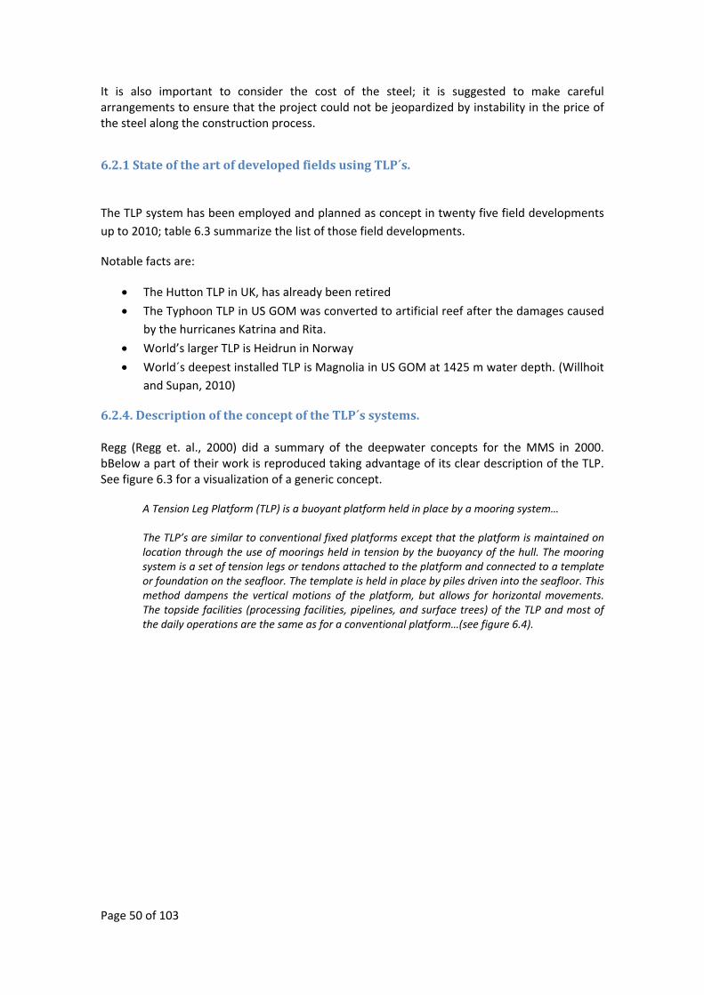
Page 50 of 103
It is also important to consider the cost of the steel; it is suggested to make careful arrangements to ensure that the project could not be jeopardized by instability in the price of the steel along the construction process.
6.2.1 State of the art of developed fields using TLP´s.
The TLP system has been employed and planned as concept in twenty five field developments up to 2010; table 6.3 summarize the list of those field developments.
Notable facts are:
• The Hutton TLP in UK, has already been retired
• The Typhoon TLP in US GOM was converted to artificial reef after the damages caused by the hurricanes Katrina and Rita.
• World’s larger TLP is Heidrun in Norway
• World´s deepest installed TLP is Magnolia in US GOM at 1425 m water depth. (Willhoit and Supan, 2010)
6.2.4. Description of the concept of the TLP´s systems. Regg (Regg et. al., 2000) did a summary of the deepwater concepts for the MMS in 2000. bBelow a part of their work is reproduced taking advantage of its clear description of the TLP. See figure 6.3 for a visualization of a generic concept.
A Tension Leg Platform (TLP) is a buoyant platform held in place by a mooring system… The TLP’s are similar to conventional fixed platforms except that the platform is maintained on location through the use of moorings held in tension by the buoyancy of the hull. The mooring system is a set of tension legs or tendons attached to the platform and connected to a template or foundation on the seafloor. The template is held in place by piles driven into the seafloor. This method dampens the vertical motions of the platform, but allows for horizontal movements. The topside facilities (processing facilities, pipelines, and surface trees) of the TLP and most of the daily operations are the same as for a conventional platform…(see figure 6.4).
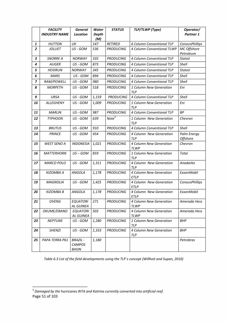
Page 51 of 103
FACILITY INDUSTRY NAME
General Location
Water Depth (M)
STATUS TLP/TLWP (Type) Operator/ Partner 1
1 HUTTON UK 147 RETIRED 6 Column Conventional TLP ConocoPhillips2 JOLLIET US ‐ GOM
536 PRODUCING 4 Column Conventional TLWP MC Offshore
Petroleum 3 SNORRE A NORWAY 335 PRODUCING 4 Column Conventional TLP Statoil
4 AUGER US ‐ GOM 873 PRODUCING 4 Column Conventional TLP Shell
5 HEIDRUN NORWAY 345 PRODUCING 4 Column Conventional TLP Statoil
6 MARS US ‐ GOM 894 PRODUCING 4 Column Conventional TLP Shell
7 RAM/POWELL US ‐ GOM 980 PRODUCING 4 Column Conventional TLP Shell
8 MORPETH US ‐ GOM 518 PRODUCING 1 Column New Generation TLP
Eni
9 URSA US ‐ GOM 1,159 PRODUCING 4 Column Conventional TLP Shell
10 ALLEGHENY US ‐ GOM 1,009 PRODUCING 1 Column New Generation TLP
Eni
11 MARLIN US ‐ GOM 987 PRODUCING 4 Column Conventional TLP BP
12 TYPHOON US ‐ GOM 639 Note4 1 Column New Generation TLP
Chevron
13 BRUTUS US ‐ GOM 910 PRODUCING 4 Column Conventional TLP Shell
14 PRINCE US ‐ GOM 454 PRODUCING 4 Column New Generation TLP
Palm Energy Offshore
15 WEST SENO A INDONESIA 1,021 PRODUCING 4 Column New Generation TLWP
Chevron
16 MATTERHORN US – GOM 859 PRODUCING 1 Column New Generation TLP
Total
17 MARCO POLO US ‐ GOM
1,311 PRODUCING 4 Column New Generation TLP
Anadarko
18 KIZOMBA A ANGOLA 1,178 PRODUCING 4 Column New Generation ETLP
ExxonMobil
19 MAGNOLIA US ‐ GOM
1,425 PRODUCING 4 Column New Generation ETLP
ConocoPhillips
20 KIZOMBA B ANGOLA 1,178 PRODUCING 4 Column New Generation ETLP
ExxonMobil
21 OVENG EQUATORIAL GUINEA
271 PRODUCING 4 Column New Generation TLWP
Amerada Hess
22 OKUME/EBANO EQUATORIAL GUINEA
503 PRODUCING 4 Column New Generation TLWP
Amerada Hess
23 NEPTUNE US ‐ GOM 1,280 PRODUCING 1 Column New Generation TLP
BHP
24 SHENZI US ‐ GOM
1,333 PRODUCING 4 Column New Generation TLP
BHP
25 PAPA TERRA P61 BRAZIL ‐CAMPOS BASIN
1,180
Petrobras
Table 6.3 List of the field developments using the TLP´s concept (Willhoit and Supan, 2010)
4 Damaged by the hurricanes RITA and Katrina currently converted into artificial reef.
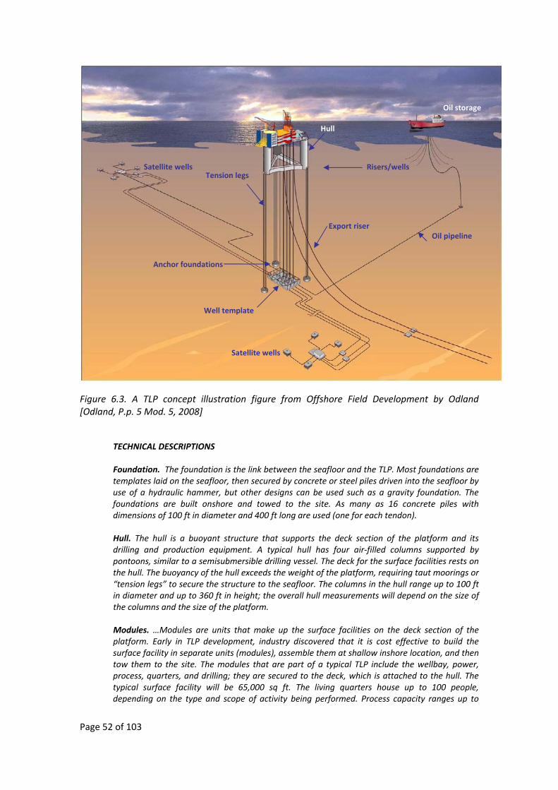
Page 52 of 103
Figure 6.3. A TLP concept illustration figure from Offshore Field Development by Odland [Odland, P.p. 5 Mod. 5, 2008]
TECHNICAL DESCRIPTIONS Foundation. The foundation is the link between the seafloor and the TLP. Most foundations are templates laid on the seafloor, then secured by concrete or steel piles driven into the seafloor by use of a hydraulic hammer, but other designs can be used such as a gravity foundation. The foundations are built onshore and towed to the site. As many as 16 concrete piles with dimensions of 100 ft in diameter and 400 ft long are used (one for each tendon). Hull. The hull is a buoyant structure that supports the deck section of the platform and its drilling and production equipment. A typical hull has four air‐filled columns supported by pontoons, similar to a semisubmersible drilling vessel. The deck for the surface facilities rests on the hull. The buoyancy of the hull exceeds the weight of the platform, requiring taut moorings or “tension legs” to secure the structure to the seafloor. The columns in the hull range up to 100 ft in diameter and up to 360 ft in height; the overall hull measurements will depend on the size of the columns and the size of the platform. Modules. …Modules are units that make up the surface facilities on the deck section of the platform. Early in TLP development, industry discovered that it is cost effective to build the surface facility in separate units (modules), assemble them at shallow inshore location, and then tow them to the site. The modules that are part of a typical TLP include the wellbay, power, process, quarters, and drilling; they are secured to the deck, which is attached to the hull. The typical surface facility will be 65,000 sq ft. The living quarters house up to 100 people, depending on the type and scope of activity being performed. Process capacity ranges up to
Tension legs
Well template
Anchor foundations
Export riser
Oil storage
Oil pipeline
Risers/wells
Hull
Satellite wells
Satellite wells
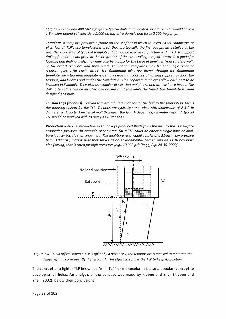
Page 53 of 103
Fx
T
a
No load position
di Fz
Setdown
Offset x
150,000 BPD oil and 400 MMscfd gas. A typical drilling rig located on a larger TLP would have a 1.5 million‐pound pull derrick, a 2,000‐hp top‐drive derrick, and three 2,200‐hp pumps. Template. A template provides a frame on the seafloor in which to insert either conductors or piles. Not all TLP’s use templates; if used, they are typically the first equipment installed at the site. There are several types of templates that may be used in conjunction with a TLP to support drilling foundation integrity, or the integration of the two. Drilling templates provide a guide for locating and drilling wells; they may also be a base for the tie‐in of flowlines from satellite wells or for export pipelines and their risers. Foundation templates may be one single piece or separate pieces for each corner. The foundation piles are driven through the foundation template. An integrated template is a single piece that contains all drilling support, anchors the tendons, and locates and guides the foundation piles. Separate templates allow each part to be installed individually. They also use smaller pieces that weigh less and are easier to install. The drilling template can be installed and drilling can begin while the foundation template is being designed and built. Tension Legs (tendons). Tension legs are tubulars that secure the hull to the foundation; this is the mooring system for the TLP. Tendons are typically steel tubes with dimensions of 2‐3 ft in diameter with up to 3 inches of wall thickness, the length depending on water depth. A typical TLP would be installed with as many as 16 tendons. Production Risers. A production riser conveys produced fluids from the well to the TLP surface production facilities. An example riser system for a TLP could be either a single‐bore or dual‐bore (concentric pipe) arrangement. The dual‐bore riser would consist of a 21‐inch, low pressure (e.g., 3,000 psi) marine riser that serves as an environmental barrier, and an 11 ¾‐inch inner pipe (casing) that is rated for high pressures (e.g., 10,000 psi) [Regg, P.p. 28‐30, 2000].
Figure 6.4. TLP in offset. When a TLP is offset by a distance x, the tendons are supposed to maintain the length di, and consequently the tension T. This effect will cause the TLP to keep its position.
The concept of a lighter TLP known as “mini TLP” or monocolumn is also a popular concept to develop small fields. An analysis of the concept was made by Kibbee and Snell (Kibbee and Snell, 2002), below their conclusions:
Page 54 of 103
This section draws conclusions from project experience and future plans for expanding the capabilities of mono‐column TLP’s.
1. The successful installation and operation of SeaStar TLP’s in the Morpeth, Allegheny, and Typhoon fields demonstrates that tension‐leg moorings provide a reliable, cost‐effective, and compact means for providing safe and stable real estate in deep water, regardless of the operator’s choice of completion type (i.e., wet‐tree or dry‐tree). The tension‐leg mooring makes it possible for smaller, less expensive hulls to be stable with favorable motion characteristics. The elimination of vertical motion not only makes dry‐trees feasible, but it also expands SCR applicability, simplifies production operations, and increases personnel comfort and safety.
2. The mono‐column hull has proven its versatility in all project phases:
• Design: Mono‐column hull sizes continue to increase to support increasing payloads. Between standard designs, it is possible to increase payload capacity by adding a column extension, thereby avoiding extensive hull structural redesign.
• Fabrication: SeaStar’s modular nature allows it to be efficiently built in relatively small fabrication yards, thereby increasing competition.
• Installation: The monocolumn hull can be wet‐towed or dry‐towed. Smaller hulls, like Morpeth, Allegheny, and Typhoon can be lifted and installed much like a vertically lifted jacket. Larger hulls, like Matterhorn, can be wettowed. Major innovations are underway to reduce dependence on derrick barges.
• Operations: There are no holes below the waterline in a SeaStar hull, eliminating the possibility of accidental flooding due to pilot error.
3. Like the mono‐column fixed base platform, the monocolumn TLP will continue to evolve based on field experience and new requirements. The standardized nature of the monocolumn TLP product avoids the inefficiency of starting with “a blank sheet of paper” on each project, while still providing the benefit of product‐focused lessons learned and execution systems. Atlantia’s continuous involvement in platform performance monitoring provides a wealth of knowledge that can be used to validate design tools and improve design details. [Kibbee et. al. P.p. 4‐5, 2002].
6.2.5. Benefits and challenges for the TLP concept.
Odland made a summary of the characteristics of the TLP concept during his class at the University of Stavanger [Odland, 2008]. He stated that the TLP concept is well‐known, but needs a careful design of its hull and mooring configuration. It has a complex dynamic behavior but is suitable for deep water. The wells are located over the platform, which increase the capability for increased oil recovery. A challenge to manage is also the, top‐tensioned (exposed) rigid risers.
Its installation and decommissioning presuppose comprehensive and complex marine operations, however, it is possible to do the installation of the topsides at shore. The concept is not suitable for oil storage. Last but not least, subject of main concern is the action of the Hurricanes in the Gulf of Mexico, the recent effects of Katrina, Lili, Ivan, etc. allowed research on the effects of the environmental loads on floating structures including the TLP.
Page 55 of 103
SECOND PART: DEVELOPMENT, CONCLUSIONS AND RECOMMENDATIONS
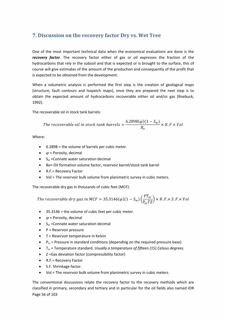
Page 56 of 103
7. Discussion on the recovery factor Dry vs. Wet Tree
One of the most important technical data when the economical evaluations are done is the recovery factor. The recovery factor either of gas or oil expresses the fraction of the hydrocarbons that rely in the subsoil and that is expected or is brought to the surface, this of course will give estimates of the amount of the production and consequently of the profit that is expected to be obtained from the development.
When a volumetric analysis is performed the first step is the creation of geological maps (structure, fault contours and Isopatch maps), once they are prepared the next step is to obtain the expected amount of hydrocarbons recoverable either oil and/or gas (Roebuck, 1992).
The recoverable oil in stock tank barrels:
6.2898 1
. .
Where:
• 6.2898 = the volume of barrels per cubic meter.
• = Porosity, decimal
• Sw =Connate water saturation decimal
• Bo= Oil formation volume factor, reservoir barrel/stock tank barrel
• R.F.= Recovery Factor
• Vol = The reservoir bulk volume from planimetric survey in cubic meters.
The recoverable dry gas in thousands of cubic feet (MCF):
35.3146 1 . . . .
• 35.3146 = the volume of cubic feet per cubic meter.
• = Porosity, decimal
• Sw =Connate water saturation decimal
• P = Reservoir pressure
• T = Reservoir temperature in Kelvin
• Psc = Pressure in standard conditions (depending on the required pressure base)
• Tsc = Temperature standard. Usually a temperature of fifteen (15) Celsius degrees.
• Z =Gas deviation factor (compressibility factor)
• R.F.= Recovery Factor
• S.F. Shrinkage factor.
• Vol = The reservoir bulk volume from planimetric survey in cubic meters.
The conventional discussions relate the recovery factor to the recovery methods which are classified in primary, secondary and tertiary and in particular for the oil fields also named IOR
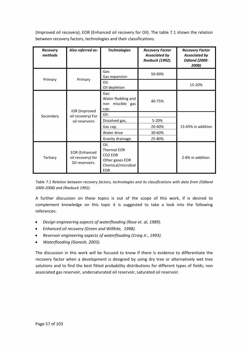
Page 57 of 103
(Improved oil recovery), EOR (Enhanced oil recovery for Oil). The table 7.1 shown the relation between recovery factors, technologies and their classifications.
Recovery methods
Also referred as: Technologies Recovery Factor Associated by Roebuck (1992).
Recovery Factor Associated by Odland (2000‐
2008)
Primary Primary
Gas: Gas expansion
50‐90%
Oil: Oil depletion
15‐20%
Secondary IOR (Improved oil recovery) For oil reservoirs
Gas: Water flodding and non miscible gas cap.
40‐75%
Oil:
15‐45% in addition
Dissolved gas, 5‐20%
Gas cap, 20‐40%
Water drive 30‐60%
Gravity drainage. 25‐80%
Tertiary EOR (Enhanced oil recovery) for Oil reservoirs.
Oil. Thermal EOR CO2 EOR Other gases EOR Chemical/microbial EOR
2‐8% in addition.
Table 7.1 Relation between recovery factors, technologies and its classifications with data from (Odland 2000‐2008) and (Roebuck 1992).
A further discussion on these topics is out of the scope of this work, if is desired to complement knowledge on this topic it is suggested to take a look into the following references:
• Design engineering aspects of waterflooding (Rose et. al, 1989).
• Enhanced oil recovery (Green and Willhite, 1998).
• Reservoir engineering aspects of waterflooding (Craig Jr., 1993).
• Waterflooding (Ganesh, 2003).
The discussion in this work will be focused to know if there is evidence to differentiate the recovery factor when a development is designed by using dry tree or alternatively wet tree solutions and to find the best fitted probability distributions for different types of fields; non associated gas reservoir, undersaturated oil reservoir, saturated oil reservoir.
Page 58 of 103
7.1 Empirical analysis of recovery factors in deepwater US Gulf of Mexico for dry tree vs. wet tree field development solutions.
Historically the recovery factor of the subsea production systems is perceived to be not as good as the one observed in the solutions that use dry trees. The reasons for this difference might be related to:
1. The cost of the well interventions in subsea production systems is considerable higher compared to fixed or floating platforms with work over systems since they require the mobilization of MODU’s (Mobil offshore drilling units) or drilling ships for each well location.
2. The subsea wells operate with a continual high backpressure which causes that the energy that could be used to deplete more efficiently the reservoir is instead, lost in the flow line and in the choke valves of the system. (Scott, 2004).
3. Costs of subsea developments are more sensitive to the number of wells than platform developments.
4. Recoverable reserves depend on incremental costs (Odland, 2000‐2008)
Hence for modeling the recovery factor there are two ways that are suggested according to data available and the level of complexity in which the modeling is intended to be performed:
• Empirical probability distributions of the recovery factors by general analogy for rapid tests.
• Recovery factor by factorial model analogy for deeper analysis.
7.1.1. Purpose
The model here proposed would consider that the recovery factor can be forecasted by analogy to historical values using the recovery factors reported to the MMS of the USA for the fields in deep water. These probability distributions will differentiate the recovery factor when a field is developed with subsea or dry trees in the case of dominant reservoir types:
• Non associate gas reservoir.
• Undersaturated oil reservoir.
• Saturated oil reservoir.
This model is intended to be used for analysis on the Mexican side of the Gulf of Mexico; hence the historical evidence that can be inferred from the statistics of the North of the Gulf of Mexico is considered to be a suitable analogy.
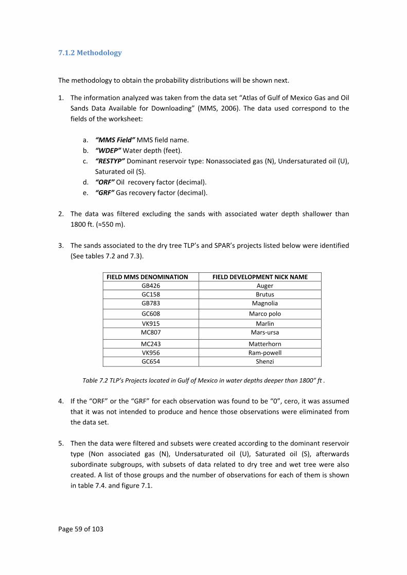
Page 59 of 103
7.1.2 Methodology
The methodology to obtain the probability distributions will be shown next.
1. The information analyzed was taken from the data set “Atlas of Gulf of Mexico Gas and Oil Sands Data Available for Downloading” (MMS, 2006). The data used correspond to the fields of the worksheet:
a. “MMS Field” MMS field name. b. “WDEP” Water depth (feet). c. “RESTYP” Dominant reservoir type: Nonassociated gas (N), Undersaturated oil (U),
Saturated oil (S). d. “ORF” Oil recovery factor (decimal). e. “GRF” Gas recovery factor (decimal).
2. The data was filtered excluding the sands with associated water depth shallower than 1800 ft. (≈550 m).
3. The sands associated to the dry tree TLP’s and SPAR’s projects listed below were identified
(See tables 7.2 and 7.3).
FIELD MMS DENOMINATION FIELD DEVELOPMENT NICK NAME GB426 AugerGC158 BrutusGB783 Magnolia
GC608 Marco polo
VK915 MarlinMC807 Mars‐ursa
MC243 MatterhornVK956 Ram‐powellGC654 Shenzi
Table 7.2 TLP’s Projects located in Gulf of Mexico in water depths deeper than 1800” ft .
4. If the “ORF” or the “GRF” for each observation was found to be “0”, cero, it was assumed
that it was not intended to produce and hence those observations were eliminated from the data set.
5. Then the data were filtered and subsets were created according to the dominant reservoir
type (Non associated gas (N), Undersaturated oil (U), Saturated oil (S), afterwards subordinate subgroups, with subsets of data related to dry tree and wet tree were also created. A list of those groups and the number of observations for each of them is shown in table 7.4. and figure 7.1.
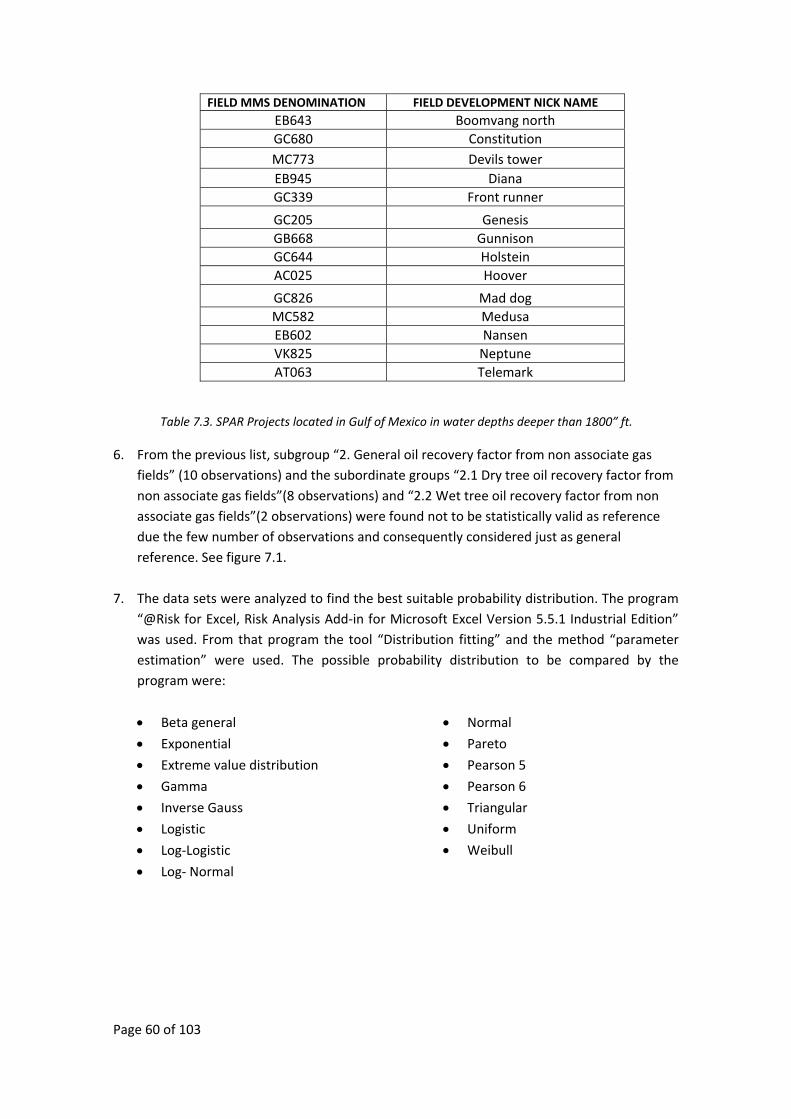
Page 60 of 103
FIELD MMS DENOMINATION FIELD DEVELOPMENT NICK NAME EB643 Boomvang north GC680 Constitution MC773 Devils tower EB945 Diana GC339 Front runner
GC205 Genesis GB668 Gunnison GC644 Holstein AC025 Hoover
GC826 Mad dog MC582 Medusa EB602 Nansen VK825 Neptune AT063 Telemark
Table 7.3. SPAR Projects located in Gulf of Mexico in water depths deeper than 1800” ft.
6. From the previous list, subgroup “2. General oil recovery factor from non associate gas fields” (10 observations) and the subordinate groups “2.1 Dry tree oil recovery factor from non associate gas fields”(8 observations) and “2.2 Wet tree oil recovery factor from non associate gas fields”(2 observations) were found not to be statistically valid as reference due the few number of observations and consequently considered just as general reference. See figure 7.1.
7. The data sets were analyzed to find the best suitable probability distribution. The program “@Risk for Excel, Risk Analysis Add‐in for Microsoft Excel Version 5.5.1 Industrial Edition” was used. From that program the tool “Distribution fitting” and the method “parameter estimation” were used. The possible probability distribution to be compared by the program were:
• Beta general
• Exponential
• Extreme value distribution
• Gamma
• Inverse Gauss
• Logistic
• Log‐Logistic
• Log‐ Normal
• Normal
• Pareto
• Pearson 5
• Pearson 6
• Triangular
• Uniform
• Weibull
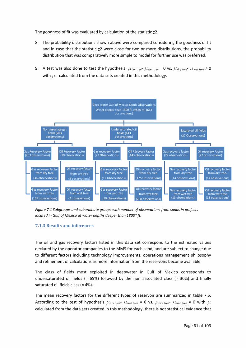
Page 61 of 103
The goodness of fit was evaluated by calculation of the statistic χ2.
8. The probability distributions shown above were compared considering the goodness of fit and in case that the statistic χ2 were close for two or more distributions, the probability distribution that was comparatively more simple to model for further use was preferred.
9. A test was also done to test the hypothesis: mdry tree‐ mwet tree = 0 vs. mdry tree‐ mwet tree ≠ 0
with m calculated from the data sets created in this methodology.
Figure 7.1 Subgroups and subordinate groups with number of observations from sands in projects located in Gulf of Mexico at water depths deeper than 1800” ft.
7.1.3 Results and inferences
The oil and gas recovery factors listed in this data set correspond to the estimated values declared by the operator companies to the MMS for each sand, and are subject to change due to different factors including technology improvements, operations management philosophy and refinement of calculations as more information from the reservoirs become available
The class of fields most exploited in deepwater in Gulf of Mexico corresponds to undersaturated oil fields (≈ 65%) followed by the non associated class (≈ 30%) and finally saturated oil fields class (≈ 4%).
The mean recovery factors for the different types of reservoir are summarized in table 7.5.
According to the test of hypothesis mdry tree‐ mwet tree = 0 vs. mdry tree‐ mwet tree ≠ 0 with m
calculated from the data sets created in this methodology, there is not statistical evidence that
Deep water Gulf of Mexico Sands Observations
Water deeper than 1800 ft. (≈550 m) (663 observations)
Non associate gas fields (203
observations)
Gas Recovery Factor (203 observations)
Gas recovery Factor from dry tree
(36 observations)
Gas recovery Factor from wet tree
(167 observations)
Oil Recovery Factor (10 observations)
Oil recovery factor
from dry tree
(8 observations)
Oil recovery factor from wet tree
(2 observations)
Undersaturated oil fields (443
observations)
Gas recovery Factor (27 Observations)
Gas recovery Factor from dry tree
(17 Observations)
Gas recovery Factor from wet tree
(10 observations)
Oil REcovery Factor (443 observations)
Oil recovery factor from dry tree
(175 Observations)
Oil recovery factor
from wet tree
(268 observations)
Saturated oil fields
(27 Observations)
Gas recovery factor (27 observations)
Gas recovery factor from dry tree
(14 observations)
Gas recovery factor from wet tree
(13 observations)
Oil recovery Factor (27 observations)
Oil recovery factor from dry tree.
(14 observations)
Oil recovery factor from wet tree
(13 observations)
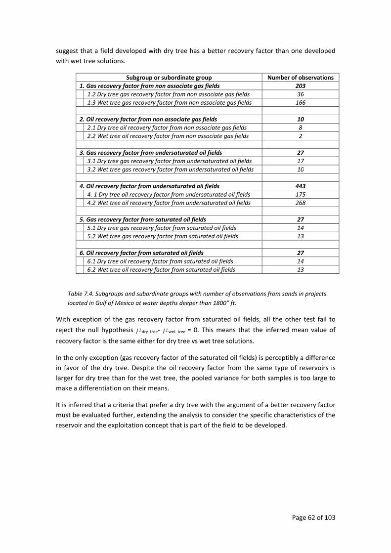
Page 62 of 103
suggest that a field developed with dry tree has a better recovery factor than one developed with wet tree solutions.
Subgroup or subordinate group Number of observations1. Gas recovery factor from non associate gas fields 203 1.2 Dry tree gas recovery factor from non associate gas fields 36 1.3 Wet tree gas recovery factor from non associate gas fields 166 2. Oil recovery factor from non associate gas fields 10 2.1 Dry tree oil recovery factor from non associate gas fields 8 2.2 Wet tree oil recovery factor from non associate gas fields 2 3. Gas recovery factor from undersaturated oil fields 27 3.1 Dry tree gas recovery factor from undersaturated oil fields 17 3.2 Wet tree gas recovery factor from undersaturated oil fields 10 4. Oil recovery factor from undersaturated oil fields 443 4. 1 Dry tree oil recovery factor from undersaturated oil fields 175 4.2 Wet tree oil recovery factor from undersaturated oil fields 268 5. Gas recovery factor from saturated oil fields 27 5.1 Dry tree gas recovery factor from saturated oil fields 14 5.2 Wet tree gas recovery factor from saturated oil fields 13 6. Oil recovery factor from saturated oil fields 27 6.1 Dry tree oil recovery factor from saturated oil fields 14 6.2 Wet tree oil recovery factor from saturated oil fields 13
Table 7.4. Subgroups and subordinate groups with number of observations from sands in projects located in Gulf of Mexico at water depths deeper than 1800” ft.
With exception of the gas recovery factor from saturated oil fields, all the other test fail to
reject the null hypothesis mdry tree‐ mwet tree = 0. This means that the inferred mean value of
recovery factor is the same either for dry tree vs wet tree solutions.
In the only exception (gas recovery factor of the saturated oil fields) is perceptibly a difference in favor of the dry tree. Despite the oil recovery factor from the same type of reservoirs is larger for dry tree than for the wet tree, the pooled variance for both samples is too large to make a differentiation on their means.
It is inferred that a criteria that prefer a dry tree with the argument of a better recovery factor must be evaluated further, extending the analysis to consider the specific characteristics of the reservoir and the exploitation concept that is part of the field to be developed.
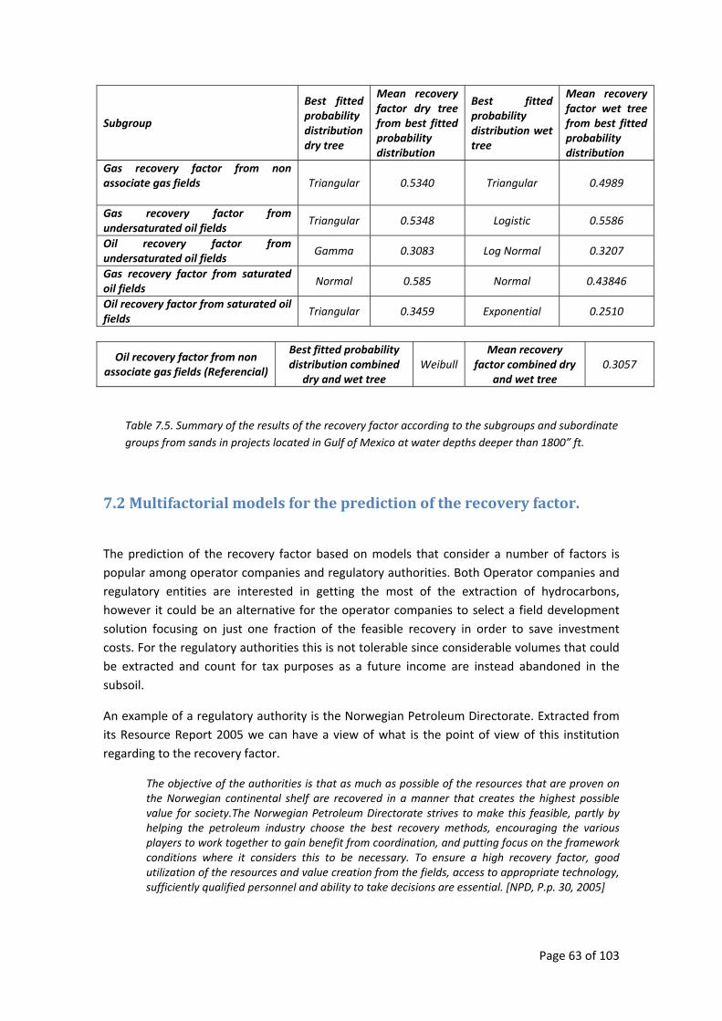
Page 63 of 103
Subgroup
Best fitted probability distribution dry tree
Mean recovery factor dry tree from best fitted probability distribution
Best fitted probability distribution wet tree
Mean recovery factor wet tree from best fitted probability distribution
Gas recovery factor from non associate gas fields
Triangular 0.5340 Triangular 0.4989
Gas recovery factor from undersaturated oil fields
Triangular 0.5348 Logistic 0.5586
Oil recovery factor from undersaturated oil fields
Gamma 0.3083 Log Normal 0.3207
Gas recovery factor from saturated oil fields
Normal 0.585 Normal 0.43846
Oil recovery factor from saturated oil fields
Triangular 0.3459 Exponential 0.2510
Oil recovery factor from non associate gas fields (Referencial)
Best fitted probability distribution combined
dry and wet tree Weibull
Mean recovery factor combined dry
and wet tree 0.3057
Table 7.5. Summary of the results of the recovery factor according to the subgroups and subordinate groups from sands in projects located in Gulf of Mexico at water depths deeper than 1800” ft.
7.2 Multifactorial models for the prediction of the recovery factor.
The prediction of the recovery factor based on models that consider a number of factors is popular among operator companies and regulatory authorities. Both Operator companies and regulatory entities are interested in getting the most of the extraction of hydrocarbons, however it could be an alternative for the operator companies to select a field development solution focusing on just one fraction of the feasible recovery in order to save investment costs. For the regulatory authorities this is not tolerable since considerable volumes that could be extracted and count for tax purposes as a future income are instead abandoned in the subsoil.
An example of a regulatory authority is the Norwegian Petroleum Directorate. Extracted from its Resource Report 2005 we can have a view of what is the point of view of this institution regarding to the recovery factor.
The objective of the authorities is that as much as possible of the resources that are proven on the Norwegian continental shelf are recovered in a manner that creates the highest possible value for society.The Norwegian Petroleum Directorate strives to make this feasible, partly by helping the petroleum industry choose the best recovery methods, encouraging the various players to work together to gain benefit from coordination, and putting focus on the framework conditions where it considers this to be necessary. To ensure a high recovery factor, good utilization of the resources and value creation from the fields, access to appropriate technology, sufficiently qualified personnel and ability to take decisions are essential. [NPD, P.p. 30, 2005]
Page 64 of 103
7.2.1 The Reservoir Complexity Index from the Norwegian petroleum directorate. Regarding the calculation of the recovery factor, the proposal of the NPD is to bench mark the recovery factor as a function of the Reservoir Complexity Index (RCI). This Index has fundament in the fact that the reservoirs have unique characteristics but if there is a way to assess the quality of the reservoirs, the complexity indicated by one measure (the reservoir complexity index, RCI) will have a strong correlation with the recovery factor expected from a development. The parameters that describe the reservoir quality according to the proposal by NPD include:
• General permeability. • Contrasts in permeability • Vertical and horizontal communications in the reservoir (influenced, for example, by
faults), • Impervious strata, • Density, • Tendency for water or gas to be drawn towards the production wells (coning) and the
like. For each parameter are given a value based on objective limits and subjective assessments. The factors are pondered and the possible value result of the index is normalized to be between 1 and 0. High values of the index mean a more complex reservoir. (NPD, 2005). Bygdevoll (Bygdevoll, 2010) did show the most important parameters found by NPD for the Norwegian fields. The scope of the study by NPD and oil companies of the Norwegian Continental Shelf considered the factors that had better correlation for its area of interest. It should not be understood that the same factors have the same relevance for all the fields around the globe. Table 7.3 reproduce the data contained in the lecture by Bygdevoll, regarding the RCI complexity attributes, its description and complexity scores.
7.2.2 Inferences about the Reservoir Complexity Index from the Norwegian petroleum directorate on the performance of dry and wet tree solutions. From the same presentation a data set was extracted for the fields encompassed by the study differentiating the dry tree and the wet tree developments. The results of the analysis of this data set are shown graphically in figure 7.2. What can be inferred from the figure 7.2 is that on the Norwegian Continental Shelf, depending of the complexity of the reservoir, there is:
A linear trend on the recovery factor for fields developed with dry tree to decrease as the reservoir becomes more complex.
An exponential trend on the recovery factor for fields developed with wet tree to decrease as the reservoir becomes more complex. A linear trend was also tested but is not shown because the exponential regressed function has a better R2 (R2 = 0.5891 in linear regression vs R2 = 0.6672 in exponential regression).
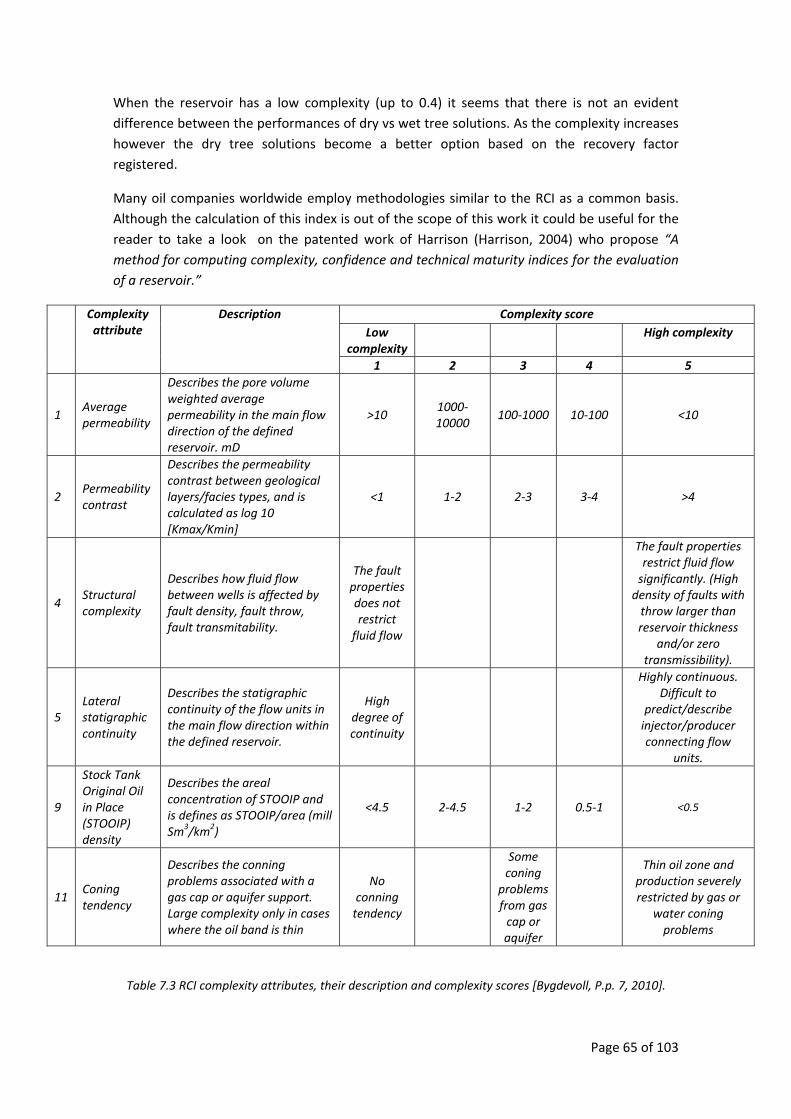
Page 65 of 103
When the reservoir has a low complexity (up to 0.4) it seems that there is not an evident difference between the performances of dry vs wet tree solutions. As the complexity increases however the dry tree solutions become a better option based on the recovery factor registered.
Many oil companies worldwide employ methodologies similar to the RCI as a common basis. Although the calculation of this index is out of the scope of this work it could be useful for the reader to take a look on the patented work of Harrison (Harrison, 2004) who propose “A method for computing complexity, confidence and technical maturity indices for the evaluation of a reservoir.”
Complexity attribute
Description Complexity score Low
complexity High complexity
1 2 3 4 5
1 Average permeability
Describes the pore volume weighted average permeability in the main flow direction of the defined reservoir. mD
>10 1000‐10000
100‐1000 10‐100 <10
2 Permeability contrast
Describes the permeability contrast between geological layers/facies types, and is calculated as log 10 [Kmax/Kmin]
<1 1‐2 2‐3 3‐4 >4
4 Structural complexity
Describes how fluid flow between wells is affected by fault density, fault throw, fault transmitability.
The fault properties does not restrict fluid flow
The fault properties restrict fluid flow significantly. (High density of faults with throw larger than reservoir thickness
and/or zero transmissibility).
5 Lateral statigraphic continuity
Describes the statigraphic continuity of the flow units in the main flow direction within the defined reservoir.
High degree of continuity
Highly continuous. Difficult to
predict/describe injector/producer connecting flow
units.
9
Stock Tank Original Oil in Place (STOOIP) density
Describes the areal concentration of STOOIP and is defines as STOOIP/area (mill Sm3/km2)
<4.5 2‐4.5 1‐2 0.5‐1 <0.5
11 Coning tendency
Describes the conning problems associated with a gas cap or aquifer support. Large complexity only in cases where the oil band is thin
No conning tendency
Some coning
problems from gas cap or aquifer
Thin oil zone and production severely restricted by gas or
water coning problems
Table 7.3 RCI complexity attributes, their description and complexity scores [Bygdevoll, P.p. 7, 2010].

Page 66 of 103
Figure 7.2 Scatter plot and a regression line showing the correlation between the recovery factors for oil from various deposits in relation to the reservoir complexity index (RCI), inferred data set from Bygdevoll, (Bygdevoll, P.p. 10, 2010]
Reservoir Complexity Index (RCI)
Recovery Factor %
Recovery factor field development, dry tree solution
Recovery factor field development, wet tree solution
Page 67 of 103
8. Models presentation
Most of the calculations were made using the “Oil and Gas Exploration Economic Model” of the Nova Scotia Department of Energy (Nova Scotia, 2008), see annex F, and the results obtained were adjusted where necessary by the “Empirical cost models for TLP’s and SPARS´s “ (Jablonowsky, 2008), and the “Models of Lifetime Cost of Subsea Production Systems, prepared for Subsea JIP, System Description & FMEA” (Goldsmith, 2000).
In this work is also proposed a way to calculate the added value of an offshore structure acting as a hub, see point 8.4.
Tax calculations are out of the scope of this work, consequently, the results will show just values before taxes.
8.1 Oil and Gas Exploration Economic Model of the Nova Scotia Department of Energy
The description of the model as given on the web page is reproduced in the next two paragraphs.
The Oil and Gas Exploration Economic Model is an excel based model designed to provide screening economics for the evaluation of oil and gas exploration prospects and discoveries on the Nova Scotian shelf in the shallow waters around Sable Island, either as tie‐ins to existing infrastructure or as stand‐alone developments, and in deep water either as stand alone or with subsea tie back to existing infrastructure.
The model provides full cycle calculations, from exploration to abandonment, and includes Nova Scotia offshore royalty and provincial and federal corporate income taxes. The government share is therefore incorporated into the cash flow and economic indicator calculations. [Nova Scotia,, P1, 2008].
A full description of the model is shown in Annex F. Since the aim of this work is to evaluate a region that is different than this model is tailored for, a modification of the input costs was necessary. Tables 8.1, 8.2 and 8.3 show the assumptions used in the economical calculations of the investments in the field developments scenarios.
8.2 Empirical Cost Model for TLP’s and SPAR’s CAPEX. Jablanowsky (Jablonowsky, 2008) presented a paper which estimates costs for SPAR’s and TLP’s projects using public and private data on 24 major projects. Besides, to provide an analysis of the variables that affect costs, the paper investigates the complexity of regression model specification in a decision‐making setting. He also evaluates the sensitivity to modeling assumptions, sample selection bias, and other model specification issues.
When the models from point 8.2 and also 8.3 were used, a simple update in the costs was made using the “IHS CERA Upstream Capital Costs Index (UCCI)”. The IHS CERA UCCI tracks the costs of equipment, facilities, materials, and personnel (both skilled and unskilled) used in the construction of a geographically diversified portfolio of twenty eight onshore, offshore, pipeline and LNG projects. It is similar to the consumer price index (CPI) in that it provides a
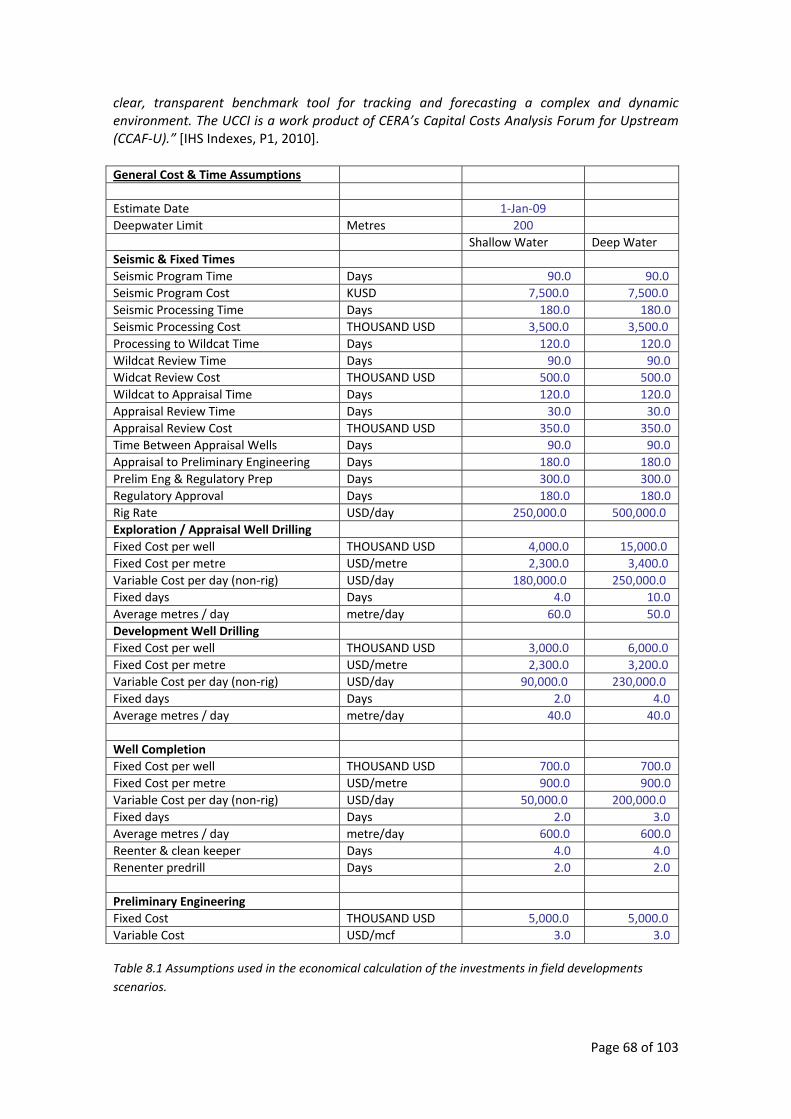
Page 68 of 103
clear, transparent benchmark tool for tracking and forecasting a complex and dynamic environment. The UCCI is a work product of CERA’s Capital Costs Analysis Forum for Upstream (CCAF‐U).” [IHS Indexes, P1, 2010].
General Cost & Time Assumptions
Estimate Date 1‐Jan‐09 Deepwater Limit Metres 200
Shallow Water Deep WaterSeismic & Fixed Times Seismic Program Time Days 90.0 90.0 Seismic Program Cost KUSD 7,500.0 7,500.0 Seismic Processing Time Days 180.0 180.0 Seismic Processing Cost THOUSAND USD 3,500.0 3,500.0 Processing to Wildcat Time Days 120.0 120.0 Wildcat Review Time Days 90.0 90.0 Widcat Review Cost THOUSAND USD 500.0 500.0 Wildcat to Appraisal Time Days 120.0 120.0 Appraisal Review Time Days 30.0 30.0 Appraisal Review Cost THOUSAND USD 350.0 350.0 Time Between Appraisal Wells Days 90.0 90.0 Appraisal to Preliminary Engineering Days 180.0 180.0 Prelim Eng & Regulatory Prep Days 300.0 300.0 Regulatory Approval Days 180.0 180.0 Rig Rate USD/day 250,000.0 500,000.0 Exploration / Appraisal Well Drilling Fixed Cost per well THOUSAND USD 4,000.0 15,000.0 Fixed Cost per metre USD/metre 2,300.0 3,400.0 Variable Cost per day (non‐rig) USD/day 180,000.0 250,000.0 Fixed days Days 4.0 10.0 Average metres / day metre/day 60.0 50.0 Development Well Drilling Fixed Cost per well THOUSAND USD 3,000.0 6,000.0 Fixed Cost per metre USD/metre 2,300.0 3,200.0 Variable Cost per day (non‐rig) USD/day 90,000.0 230,000.0 Fixed days Days 2.0 4.0 Average metres / day metre/day 40.0 40.0
Well Completion Fixed Cost per well THOUSAND USD 700.0 700.0 Fixed Cost per metre USD/metre 900.0 900.0 Variable Cost per day (non‐rig) USD/day 50,000.0 200,000.0 Fixed days Days 2.0 3.0 Average metres / day metre/day 600.0 600.0 Reenter & clean keeper Days 4.0 4.0 Renenter predrill Days 2.0 2.0
Preliminary Engineering Fixed Cost THOUSAND USD 5,000.0 5,000.0 Variable Cost USD/mcf 3.0 3.0 Table 8.1 Assumptions used in the economical calculation of the investments in field developments scenarios.
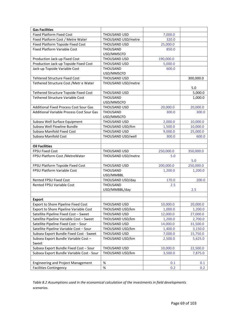
Page 69 of 103
Gas Facilities Fixed Platform Fixed Cost THOUSAND USD 7,000.0 Fixed Platform Cost / Metre Water THOUSAND USD/metre 320.0 Fixed Platform Topside Fixed Cost THOUSAND USD 25,000.0 Fixed Platform Variable Cost THOUSAND
USD/MMSCFD 850.0
Production Jack‐up Fixed Cost THOUSAND USD 190,000.0 Production Jack‐up Topside Fixed Cost THOUSAND USD 5,000.0 Jack‐up Topside Variable Cost THOUSAND
USD/MMSCFD 600.0
Tehtered Structure Fixed Cost THOUSAND USD 300,000.0 Tethered Structure Cost /Metr e Water THOUSAND USD/metre
5.0 Tethered Structure Topside Fixed Cost THOUSAND USD 5,000.0 Tethered Structure Variable Cost THOUSAND
USD/MMSCFD 1,000.0
Additional Fixed Process Cost Sour Gas THOUSAND USD 20,000.0 20,000.0 Additional Variable Process Cost Sour Gas THOUSAND
USD/MMSCFD 300.0 300.0
Subsea Well Surface Equipment THOUSAND USD 2,000.0 10,000.0 Subsea Well Flowline Bundle THOUSAND USD/Km 1,500.0 10,000.0 Subsea Manifold Fixed Cost THOUSAND USD 9,000.0 25,000.0 Subsea Manifold Cost THOUSAND USD/well 300.0 600.0
Oil Facilities FPSU Fixed Cost THOUSAND USD 250,000.0 350,000.0 FPSU Platform Cost /MetreWater THOUSAND USD/metre 5.0
5.0 FPSU Platform Topside Fixed Cost THOUSAND USD 200,000.0 250,000.0 FPSU Platform Variable Cost THOUSAND
USD/MMBBL 1,200.0 1,200.0
Rented FPSU Fixed Cost THOUSAND USD/day 170.0 200.0 Rented FPSU Variable Cost THOUSAND
USD/MMBBL/day 2.5
2.5
Export Export to Shore Pipeline Fixed Cost THOUSAND USD 10,000.0 20,000.0 Export to Shore Pipeline Variable Cost THOUSAND USD/km 1,000.0 1,200.0 Satellite Pipeline Fixed Cost – Sweet THOUSAND USD 12,000.0 27,000.0 Satellite Pipeline Variable Cost – Sweet THOUSAND USD/km 1,200.0 2,700.0 Satellite Pipeline Fixed Cost – Sour THOUSAND USD 14,000.0 31,500.0 Satellite Pipeline Variable Cost – Sour THOUSAND USD/km 1,400.0 3,150.0 Subsea Export Bundle Fixed Cost ‐ Sweet THOUSAND USD 7,000.0 15,750.0 Subsea Export Bundle Variable Cost – Sweet
THOUSAND USD/km 2,500.0 5,625.0
Subsea Export Bundle Fixed Cost – Sour THOUSAND USD 10,000.0 22,500.0 Subsea Export Bundle Variable Cost ‐ Sour THOUSAND USD/km 3,500.0 7,875.0
Engineering and Project Management % 0.1 0.1 Facilities Contingency % 0.2 0.2
Table 8.2 Assumptions used in the economical calculation of the investments in field developments scenarios.
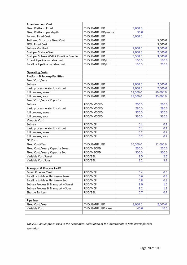
Page 70 of 103
Abandonment Cost Fixed Platform Fixed THOUSAND USD 3,000.0 Fixed Platform per depth THOUSAND USD/metre 30.0 Jack‐up Fixed Cost THOUSAND USD 5,000.0 Tethered Structure Fixed Cost THOUSAND USD 5,000.0 FPSU Fixed Cost THOUSAND USD 5,000.0 Subsea Manifold THOUSAND USD 2,000.0 3,000.0 Cost per Surface Well THOUSAND USD 2,000.0 2,000.0 Cost per Subsea Well & Flowline Bundle THOUSAND USD 3,500.0 3,500.0 Export Pipeline variable cost THOUSAND USD/km 100.0 100.0 Satellite Pipeline variable cost THOUSAND USD/km 150.0 250.0
Operating Costs Platform & Jack‐up Facilities Fixed Cost /Year Subsea THOUSAND USD 2,000.0 2,000.0 basic process, water knock out THOUSAND USD 7,000.0 7,000.0 full process, sweet THOUSAND USD 19,000.0 19,000.0 full process, sour THOUSAND USD 25,000.0 25,000.0 Fixed Cost /Year / Capacity Subsea USD/MMSCFD 200.0 200.0 basic process, water knock out USD/MMSCFD 280.0 280.0 full process, sweet USD/MMSCFD 370.0 370.0 full process, sour USD/MMSCFD 530.0 530.0 Variable Cost Subsea USD/MCF 0.1 0.1 basic process, water knock out USD/MCF 0.1 0.1 full process, sweet USD/MCF 0.2 0.2 full process, sour USD/MCF 0.2 0.2 Oil Costs Fixed Cost/Year THOUSAND USD 10,000.0 12,000.0 Fixed Cost /Year / Capacity Sweet USD/MBOPD 250.0 250.0 Fixed Cost /Year / Capacity Sour USD/MBOPD 300.0 300.0 Variable Cost Sweet USD/BBL 2.5 2.5 Variable Cost Sour USD/BBL 3.2 3.2
Transport & Process Tariff Direct Pipeline Tie‐in USD/MCF 0.4 0.4 Satellite to Main Platform – Sweet USD/MCF 0.6 0.6 Satellite to Main Platform – Sour USD/MCF 0.8 0.8 Subsea Process & Transport – Sweet USD/MCF 1.0 1.0 Subsea Process & Transport – Sour USD/MCF 1.2 1.2 Shuttle Tankers USD/BBL 0.7 0.7
Pipelines Fixed Cost /Year THOUSAND USD 2,000.0 2,000.0 Variable Cost THOUSAND USD / km 40.0 40.0
Table 8.3 Assumptions used in the economical calculation of the investments in field developments scenarios.
Page 71 of 103
8.3 Goldsmith Models for OPEX, RAMEX and RISKEX.
Reference is made to paragraph 5.3 and “Models of Lifetime Cost of Subsea Production Systems, prepared for Subsea JIP, System Description & FMEA” (Goldsmith, 2000). The RAMEX results from this report are used to correct the calculations presented in chapter 9. The RISKEX are not included because every concept development has a particular and unique set of characteristics that cause considerably different outcome scenarios and consequently different results, too complex for a first initial screening as the scope of this work considers.
8.4 Value added of a floating structure acting as a Hub
As it is show in appendix G, the activity in deep water offshore Mexico is having place in a region with an evident lack of preexisting infrastructure. This fact makes it important to develop a network of facilities that should increase the feasibility of development in the future.
Hence it is proposed here that additional offshore structures shall have an added value for comparison purposes. This added value will be calculated by doing an evaluation of NPV for the prospects that could be developed if the facility would be in place already.
To account for this added value, a series of assumptions have been considered:
1. It will be assumed that the estimated prospective resources are the real original volume in place.
2. The net present value will also be discounted by some assigned probabilities representing discovery, appraisal and development in the way that:
Accounted added value =
NPV (Development the field X Overall Chance of success)
When apply… ‐ NPV(Cost for planning development the field X Probability of pass an appraisal, given a discovery)
When apply… ‐ NPV (Cost for appraisal X Probability of a discovery)
When apply… ‐ NPV (Cost for wildcat)
Where:
Overall Chance of Success = (Probability of discovery) X (Probability to pass to appraisal given a discovery) X (Probability of develop, given an appraisal, given a discovery)
These formulas are intended to discount the uncertainty of the discovery and also the uncertainty related to pass the different decision gates mentioned in chapter 4. It will also discount the irreversible investments that occur in the field development process.
Page 72 of 103
3. The criteria to add prospects to the analysis was the distance to the proposed facility; when it was identified that there was less than 90 km in a slightly curved route, the prospect was allowed to be included in the calculations.
4. It should not be understood that all the included prospects are proposed to be tied back to the host facility since there are capability restrictions in every structure; it is just an assumption to calculate the added value of new infrastructure in the region of interest.
5. The parameters of the NPV calculation will be shown in chapter 9. As a general case, for calculation purposes, we will assume a subsea field development with a tie back to processing and a production stream induction through the offshore. In some cases an array in “daisy chain” is proposed. For many of the prospects a low probability and low forecasted resources were assumed since there was not a clear expectation related to them in the literature listed in chapter nine.
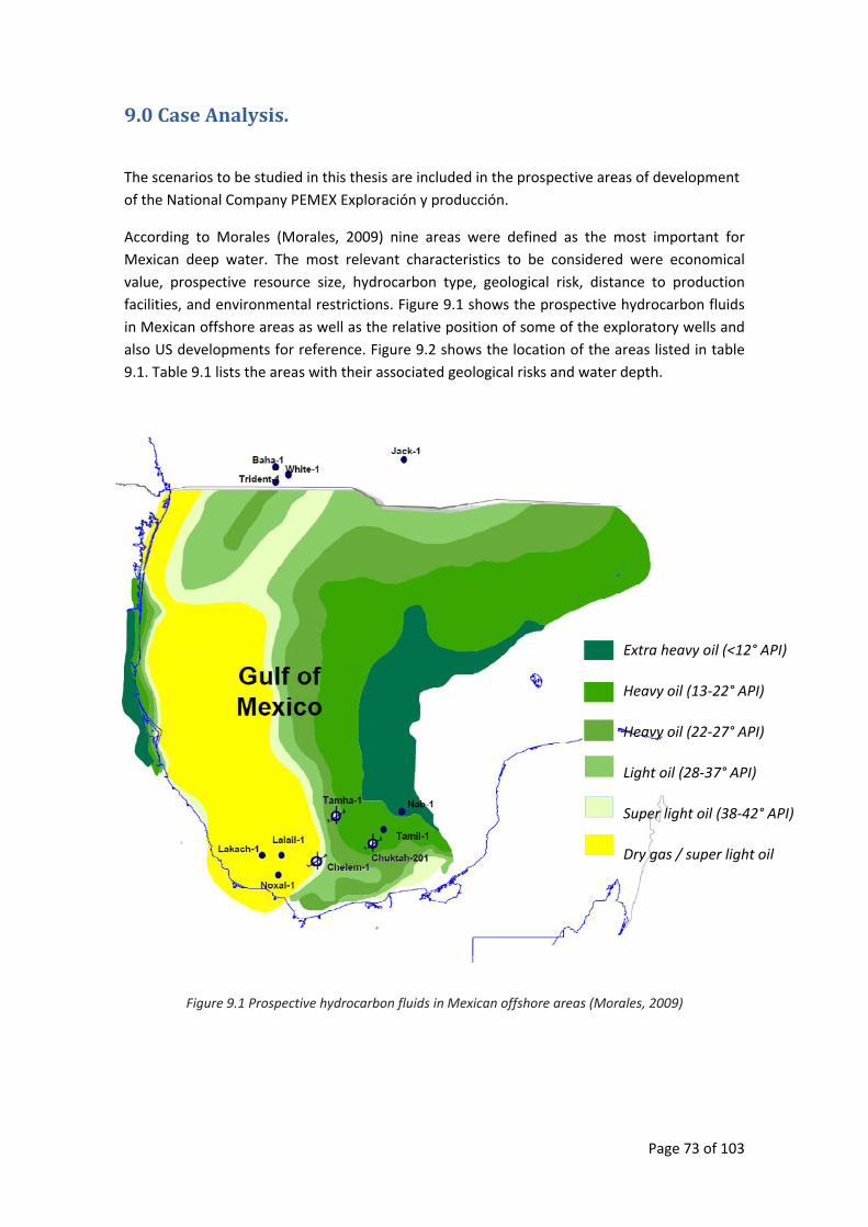
Page 73 of 103
9.0 Case Analysis.
The scenarios to be studied in this thesis are included in the prospective areas of development of the National Company PEMEX Exploración y producción.
According to Morales (Morales, 2009) nine areas were defined as the most important for Mexican deep water. The most relevant characteristics to be considered were economical value, prospective resource size, hydrocarbon type, geological risk, distance to production facilities, and environmental restrictions. Figure 9.1 shows the prospective hydrocarbon fluids in Mexican offshore areas as well as the relative position of some of the exploratory wells and also US developments for reference. Figure 9.2 shows the location of the areas listed in table 9.1. Table 9.1 lists the areas with their associated geological risks and water depth.
Figure 9.1 Prospective hydrocarbon fluids in Mexican offshore areas (Morales, 2009)
• Extra heavy oil (<12° API) • • Heavy oil (13‐22° API) • • Heavy oil (22‐27° API) • • Light oil (28‐37° API) • • Super light oil (38‐42° API) • • Dry gas / super light oil
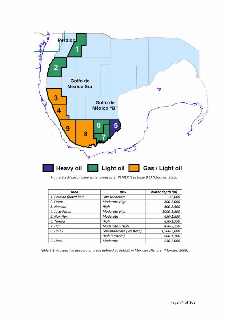
Page 74 of 103
Figure 9.2 Mexican deep water areas after PEMEX (See table 9.1).(Morales, 2009)
Area Risk Water depth (m) 1. Perdido folded belt Low‐Moderate >2,000 2. Oreos Moderate‐High 800‐2,000 3. Nancan High 500‐2,500 4. Jaca‐Patini Moderate‐High 1000‐1,500 5. Nox‐Hux Moderate 650‐1,850 6. Temoa High 850‐1,950 7. Han Moderate – High 450‐2,250 8. Holok Low‐moderate (Western) 1,500‐2,000 High (Eastern) 600‐1,100 9. Lipax Moderate 950‐2,000
Table 9.1: Prospective deepwater areas defined by PEMEX in Mexican offshore. (Morales, 2009)
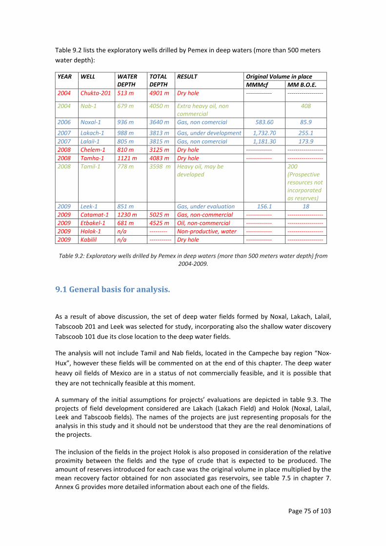
Page 75 of 103
Table 9.2 lists the exploratory wells drilled by Pemex in deep waters (more than 500 meters water depth):
YEAR WELL WATER DEPTH
TOTAL DEPTH
RESULT Original Volume in place MMMcf MM B.O.E.
2004 Chukta‐201 513 m 4901 m Dry hole ‐‐‐‐‐‐‐‐‐‐‐‐‐ ‐‐‐‐‐‐‐‐‐‐‐‐‐‐‐‐‐‐
2004 Nab‐1 679 m 4050 m Extra heavy oil, non commercial
408
2006 Noxal‐1 936 m 3640 m Gas, non comercial 583.60 85.9
2007 Lakach‐1 988 m 3813 m Gas, under development 1,732.70 255.1 2007 Lalail‐1 805 m 3815 m Gas, non comercial 1,181.30 173.9 2008 Chelem‐1 810 m 3125 m Dry hole ‐‐‐‐‐‐‐‐‐‐‐‐‐ ‐‐‐‐‐‐‐‐‐‐‐‐‐‐‐‐‐‐2008 Tamha‐1 1121 m 4083 m Dry hole ‐‐‐‐‐‐‐‐‐‐‐‐‐ ‐‐‐‐‐‐‐‐‐‐‐‐‐‐‐‐‐‐2008 Tamil‐1 778 m 3598 m Heavy oil, may be
developed 200 (Prospective resources not incorporated as reserves)
2009 Leek‐1 851 m Gas, under evaluation 156.1 18 2009 Catamat‐1 1230 m 5025 m Gas, non‐commercial ‐‐‐‐‐‐‐‐‐‐‐‐‐ ‐‐‐‐‐‐‐‐‐‐‐‐‐‐‐‐‐‐2009 Etbakel‐1 681 m 4525 m Oil, non‐commercial ‐‐‐‐‐‐‐‐‐‐‐‐‐ ‐‐‐‐‐‐‐‐‐‐‐‐‐‐‐‐‐‐2009 Holok‐1 n/a ‐‐‐‐‐‐‐‐‐ Non‐productive, water ‐‐‐‐‐‐‐‐‐‐‐‐‐ ‐‐‐‐‐‐‐‐‐‐‐‐‐‐‐‐‐‐2009 Kabilil n/a ‐‐‐‐‐‐‐‐‐‐‐ Dry hole ‐‐‐‐‐‐‐‐‐‐‐‐‐ ‐‐‐‐‐‐‐‐‐‐‐‐‐‐‐‐‐‐
Table 9.2: Exploratory wells drilled by Pemex in deep waters (more than 500 meters water depth) from
2004‐2009.
9.1 General basis for analysis.
As a result of above discussion, the set of deep water fields formed by Noxal, Lakach, Lalail, Tabscoob 201 and Leek was selected for study, incorporating also the shallow water discovery Tabscoob 101 due its close location to the deep water fields.
The analysis will not include Tamil and Nab fields, located in the Campeche bay region “Nox‐Hux”, however these fields will be commented on at the end of this chapter. The deep water heavy oil fields of Mexico are in a status of not commercially feasible, and it is possible that they are not technically feasible at this moment.
A summary of the initial assumptions for projects’ evaluations are depicted in table 9.3. The projects of field development considered are Lakach (Lakach Field) and Holok (Noxal, Lalail, Leek and Tabscoob fields). The names of the projects are just representing proposals for the analysis in this study and it should not be understood that they are the real denominations of the projects. The inclusion of the fields in the project Holok is also proposed in consideration of the relative proximity between the fields and the type of crude that is expected to be produced. The amount of reserves introduced for each case was the original volume in place multiplied by the mean recovery factor obtained for non associated gas reservoirs, see table 7.5 in chapter 7. Annex G provides more detailed information about each one of the fields.
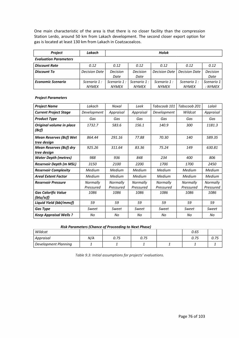
Page 76 of 103
One main characteristic of the area is that there is no closer facility than the compression Station Lerdo, around 50 km from Lakach development. The second closer export option for gas is located at least 130 km from Lakach in Coatzacoalcos.
Project Lakach Holok
Evaluation Parameters
Discount Rate 0.12 0.12 0.12 0.12 0.12 0.12
Discount To Decision Date Decision Date
Decision Date
Decision Date Decision Date Decision Date
Economic Scenario Scenario 1 : NYMEX
Scenario 1 : NYMEX
Scenario 1 : NYMEX
Scenario 1 : NYMEX
Scenario 1 : NYMEX
Scenario 1 : NYMEX
Project Parameters
Project Name Lakach Noxal Leek Tabscoob 101 Tabscoob 201 Lalail
Current Project Stage Development Appraisal Appraisal Development Wildcat Appraisal
Product Type Gas Gas Gas Gas Gas Gas
Original volume in place (Bcf)
1732.7 583.6 156.1 140.9 300 1181.3
Mean Reserves (Bcf) Wet tree design
864.44 291.16 77.88 70.30 140 589.35
Mean Reserves (Bcf) dry tree design
925.26 311.64 83.36 75.24 149 630.81
Water Depth (metres) 988 936 848 234 400 806
Reservoir Depth (m MSL) 3150 2100 2200 1700 1700 2450
Reservoir Complexity Medium Medium Medium Medium Medium Medium
Areal Extent Factor Medium Medium Medium Medium Medium Medium
Reservoir Pressure Normally Pressured
Normally Pressured
Normally Pressured
Normally Pressured
Normally Pressured
Normally Pressured
Gas Calorific Value (btu/scf)
1086 1086 1086 1086 1086 1086
Liquid Yield (bbl/mmcf) 59 59 59 59 59 59
Gas Type Sweet Sweet Sweet Sweet Sweet Sweet
Keep Appraisal Wells ? No No No No No No
Risk Parameters (Chance of Proceeding to Next Phase)Wildcat 0.65
Appraisal N/A 0.75 0.75 0.75 0.75
Development Planning 1 1 1 1 1 1
Table 9.3: Initial assumptions for projects’ evaluations.
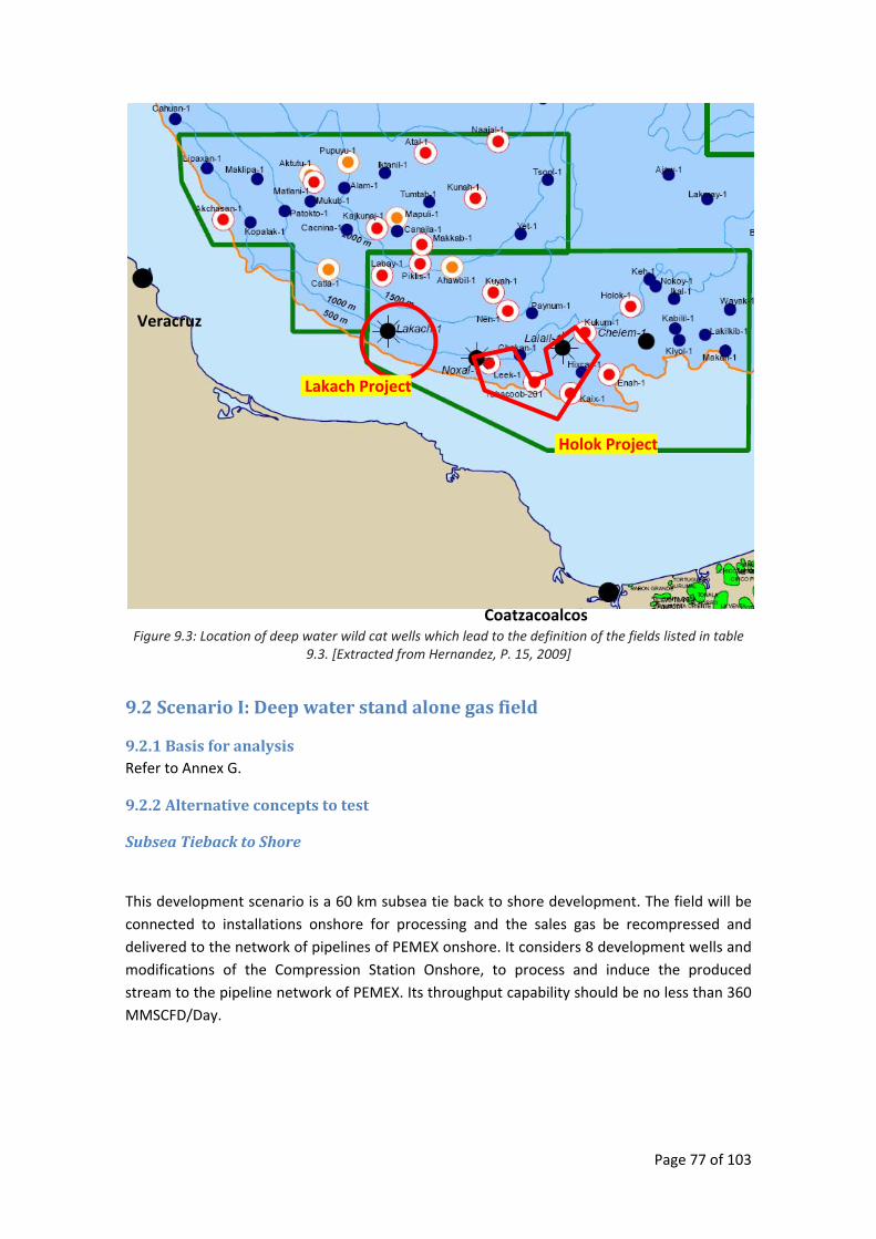
Page 77 of 103
Figure 9.3: Location of deep water wild cat wells which lead to the definition of the fields listed in table 9.3. [Extracted from Hernandez, P. 15, 2009]
9.2 Scenario I: Deep water stand alone gas field
9.2.1 Basis for analysis Refer to Annex G.
9.2.2 Alternative concepts to test
Subsea Tieback to Shore
This development scenario is a 60 km subsea tie back to shore development. The field will be connected to installations onshore for processing and the sales gas be recompressed and delivered to the network of pipelines of PEMEX onshore. It considers 8 development wells and modifications of the Compression Station Onshore, to process and induce the produced stream to the pipeline network of PEMEX. Its throughput capability should be no less than 360 MMSCFD/Day.
Lakach Project
Holok Project
Coatzacoalcos
Veracruz
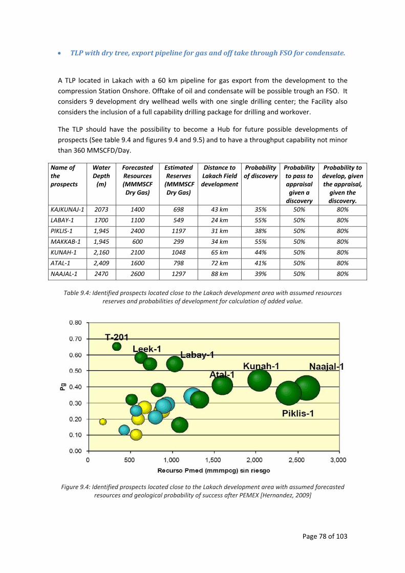
Page 78 of 103
• TLP with dry tree, export pipeline for gas and off take through FSO for condensate.
A TLP located in Lakach with a 60 km pipeline for gas export from the development to the compression Station Onshore. Offtake of oil and condensate will be possible trough an FSO. It considers 9 development dry wellhead wells with one single drilling center; the Facility also considers the inclusion of a full capability drilling package for drilling and workover.
The TLP should have the possibility to become a Hub for future possible developments of prospects (See table 9.4 and figures 9.4 and 9.5) and to have a throughput capability not minor than 360 MMSCFD/Day.
Name of the prospects
Water Depth (m)
Forecasted Resources (MMMSCF Dry Gas)
Estimated Reserves (MMMSCF Dry Gas)
Distance to Lakach Field development
Probability of discovery
Probability to pass to appraisal given a discovery
Probability to develop, given the appraisal, given the discovery.
KAJKUNAJ‐1 2073 1400 698 43 km 35% 50% 80%
LABAY‐1 1700 1100 549 24 km 55% 50% 80%
PIKLIS‐1 1,945 2400 1197 31 km 38% 50% 80%
MAKKAB‐1 1,945 600 299 34 km 55% 50% 80%
KUNAH‐1 2,160 2100 1048 65 km 44% 50% 80%
ATAL‐1 2,409 1600 798 72 km 41% 50% 80%
NAAJAL‐1 2470 2600 1297 88 km 39% 50% 80%
Table 9.4: Identified prospects located close to the Lakach development area with assumed resources
reserves and probabilities of development for calculation of added value.
Figure 9.4: Identified prospects located close to the Lakach development area with assumed forecasted
resources and geological probability of success after PEMEX [Hernandez, 2009]
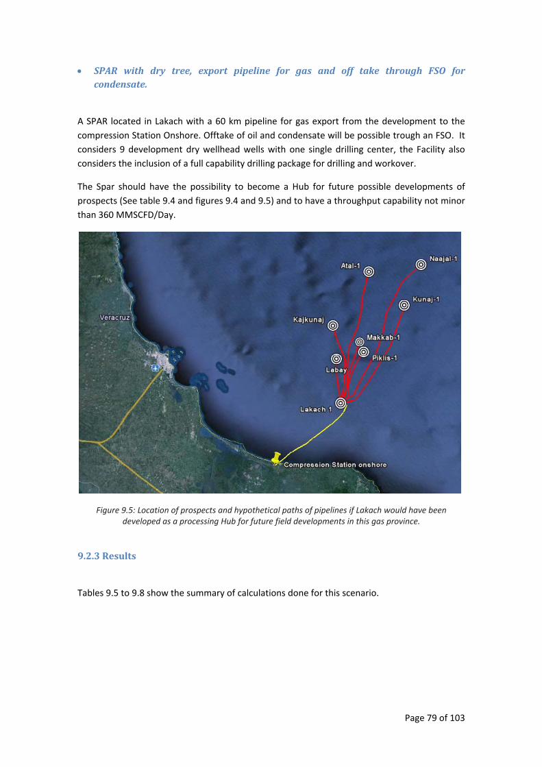
Page 79 of 103
• SPAR with dry tree, export pipeline for gas and off take through FSO for condensate.
A SPAR located in Lakach with a 60 km pipeline for gas export from the development to the compression Station Onshore. Offtake of oil and condensate will be possible trough an FSO. It considers 9 development dry wellhead wells with one single drilling center, the Facility also considers the inclusion of a full capability drilling package for drilling and workover.
The Spar should have the possibility to become a Hub for future possible developments of prospects (See table 9.4 and figures 9.4 and 9.5) and to have a throughput capability not minor than 360 MMSCFD/Day.
Figure 9.5: Location of prospects and hypothetical paths of pipelines if Lakach would have been developed as a processing Hub for future field developments in this gas province.
9.2.3 Results
Tables 9.5 to 9.8 show the summary of calculations done for this scenario.
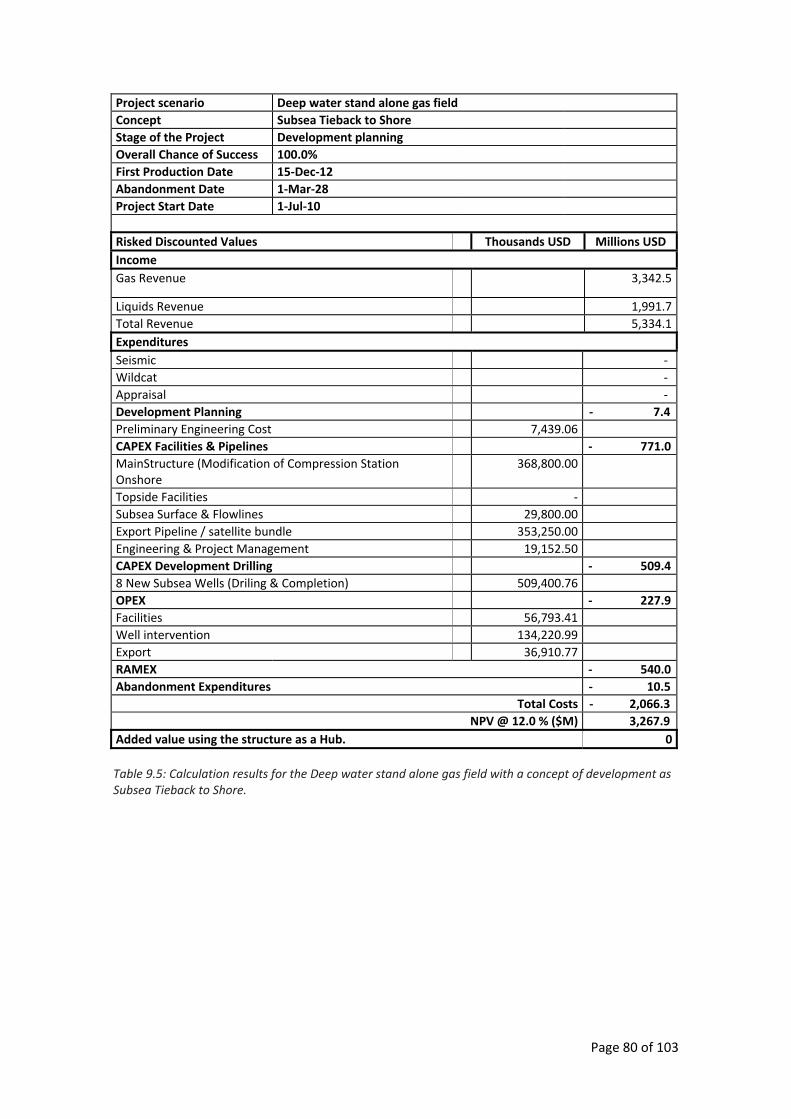
Page 80 of 103
Project scenario Deep water stand alone gas fieldConcept Subsea Tieback to Shore Stage of the Project Development planning Overall Chance of Success 100.0% First Production Date 15‐Dec‐12 Abandonment Date 1‐Mar‐28 Project Start Date 1‐Jul‐10
Risked Discounted Values Thousands USD Millions USDIncome Gas Revenue 3,342.5
Liquids Revenue 1,991.7 Total Revenue 5,334.1 Expenditures Seismic ‐ Wildcat ‐ Appraisal ‐ Development Planning ‐ 7.4 Preliminary Engineering Cost 7,439.06 CAPEX Facilities & Pipelines ‐ 771.0 MainStructure (Modification of Compression Station Onshore
368,800.00
Topside Facilities ‐ Subsea Surface & Flowlines 29,800.00 Export Pipeline / satellite bundle 353,250.00 Engineering & Project Management 19,152.50 CAPEX Development Drilling ‐ 509.4 8 New Subsea Wells (Driling & Completion) 509,400.76 OPEX ‐ 227.9 Facilities 56,793.41 Well intervention 134,220.99 Export 36,910.77 RAMEX ‐ 540.0 Abandonment Expenditures ‐ 10.5
Total Costs ‐ 2,066.3 NPV @ 12.0 % ($M) 3,267.9
Added value using the structure as a Hub. 0 Table 9.5: Calculation results for the Deep water stand alone gas field with a concept of development as Subsea Tieback to Shore.
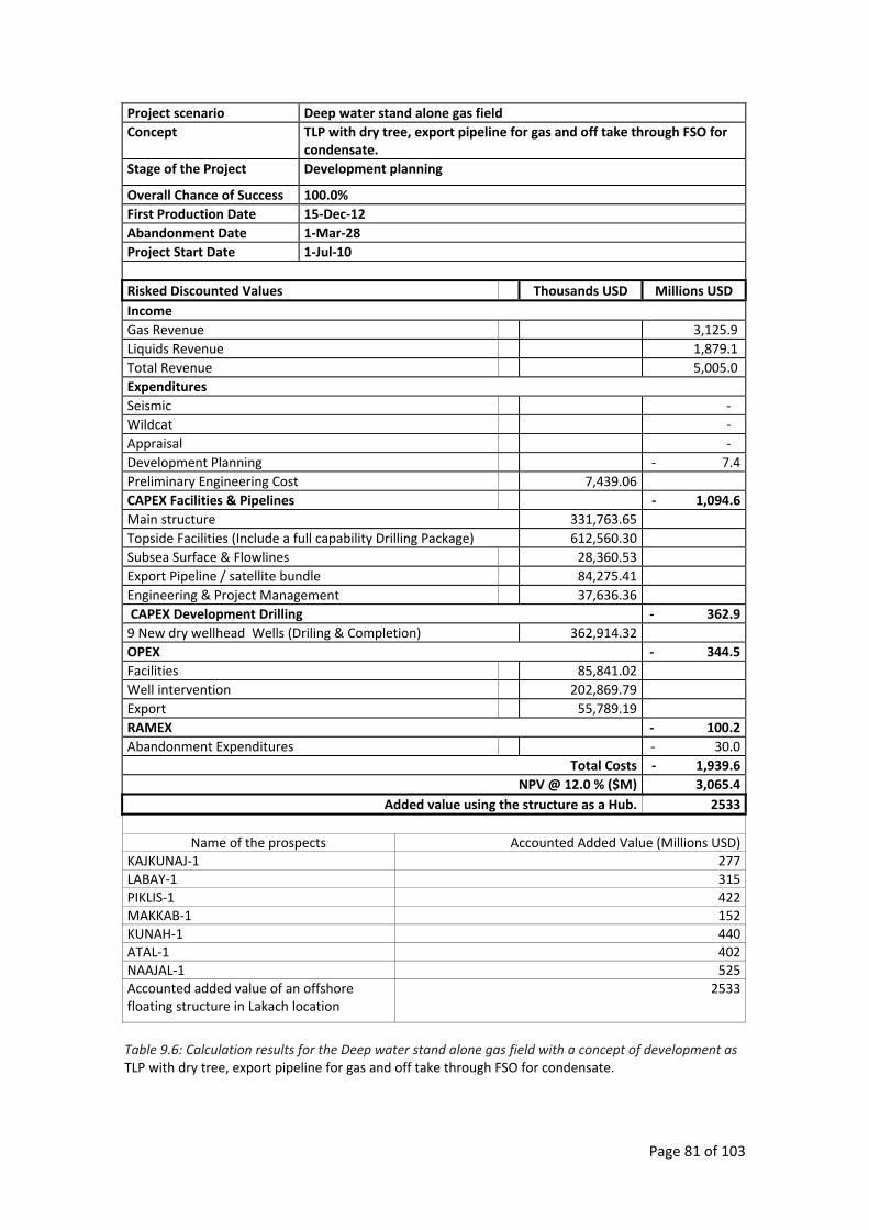
Page 81 of 103
Project scenario Deep water stand alone gas fieldConcept TLP with dry tree, export pipeline for gas and off take through FSO for
condensate. Stage of the Project Development planning
Overall Chance of Success 100.0% First Production Date 15‐Dec‐12 Abandonment Date 1‐Mar‐28 Project Start Date 1‐Jul‐10 Risked Discounted Values Thousands USD Millions USDIncome Gas Revenue 3,125.9 Liquids Revenue 1,879.1 Total Revenue 5,005.0 Expenditures Seismic ‐ Wildcat ‐ Appraisal ‐ Development Planning ‐ 7.4 Preliminary Engineering Cost 7,439.06 CAPEX Facilities & Pipelines ‐ 1,094.6 Main structure 331,763.65 Topside Facilities (Include a full capability Drilling Package) 612,560.30 Subsea Surface & Flowlines 28,360.53 Export Pipeline / satellite bundle 84,275.41 Engineering & Project Management 37,636.36 CAPEX Development Drilling ‐ 362.9 9 New dry wellhead Wells (Driling & Completion) 362,914.32 OPEX ‐ 344.5 Facilities 85,841.02 Well intervention 202,869.79 Export 55,789.19 RAMEX ‐ 100.2 Abandonment Expenditures ‐ 30.0
Total Costs ‐ 1,939.6 NPV @ 12.0 % ($M) 3,065.4
Added value using the structure as a Hub. 2533
Name of the prospects Accounted Added Value (Millions USD)KAJKUNAJ‐1 277LABAY‐1 315PIKLIS‐1 422MAKKAB‐1 152KUNAH‐1 440ATAL‐1 402NAAJAL‐1 525Accounted added value of an offshore floating structure in Lakach location
2533
Table 9.6: Calculation results for the Deep water stand alone gas field with a concept of development as TLP with dry tree, export pipeline for gas and off take through FSO for condensate.
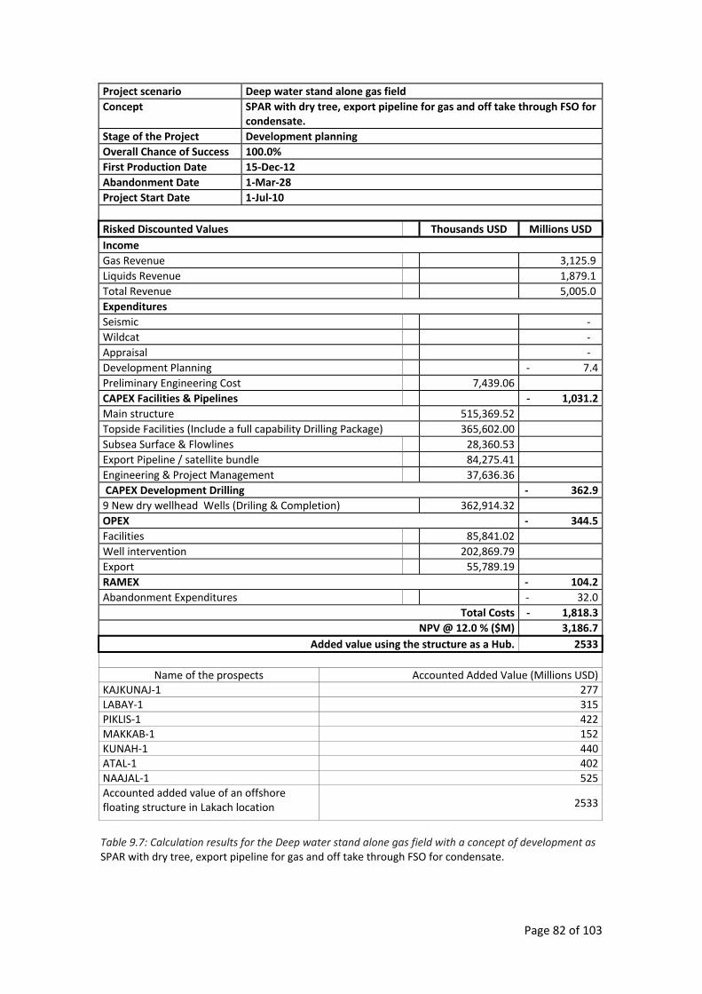
Page 82 of 103
Project scenario Deep water stand alone gas fieldConcept SPAR with dry tree, export pipeline for gas and off take through FSO for
condensate. Stage of the Project Development planning Overall Chance of Success 100.0% First Production Date 15‐Dec‐12 Abandonment Date 1‐Mar‐28 Project Start Date 1‐Jul‐10 Risked Discounted Values Thousands USD Millions USDIncome Gas Revenue 3,125.9 Liquids Revenue 1,879.1 Total Revenue 5,005.0 Expenditures Seismic ‐ Wildcat ‐ Appraisal ‐ Development Planning ‐ 7.4 Preliminary Engineering Cost 7,439.06 CAPEX Facilities & Pipelines ‐ 1,031.2Main structure 515,369.52 Topside Facilities (Include a full capability Drilling Package) 365,602.00 Subsea Surface & Flowlines 28,360.53 Export Pipeline / satellite bundle 84,275.41 Engineering & Project Management 37,636.36 CAPEX Development Drilling ‐ 362.9 9 New dry wellhead Wells (Driling & Completion) 362,914.32 OPEX ‐ 344.5 Facilities 85,841.02 Well intervention 202,869.79 Export 55,789.19 RAMEX ‐ 104.2 Abandonment Expenditures ‐ 32.0
Total Costs ‐ 1,818.3NPV @ 12.0 % ($M) 3,186.7
Added value using the structure as a Hub. 2533
Name of the prospects Accounted Added Value (Millions USD)KAJKUNAJ‐1 277LABAY‐1 315PIKLIS‐1 422MAKKAB‐1 152KUNAH‐1 440ATAL‐1 402NAAJAL‐1 525Accounted added value of an offshore floating structure in Lakach location 2533
Table 9.7: Calculation results for the Deep water stand alone gas field with a concept of development as SPAR with dry tree, export pipeline for gas and off take through FSO for condensate.
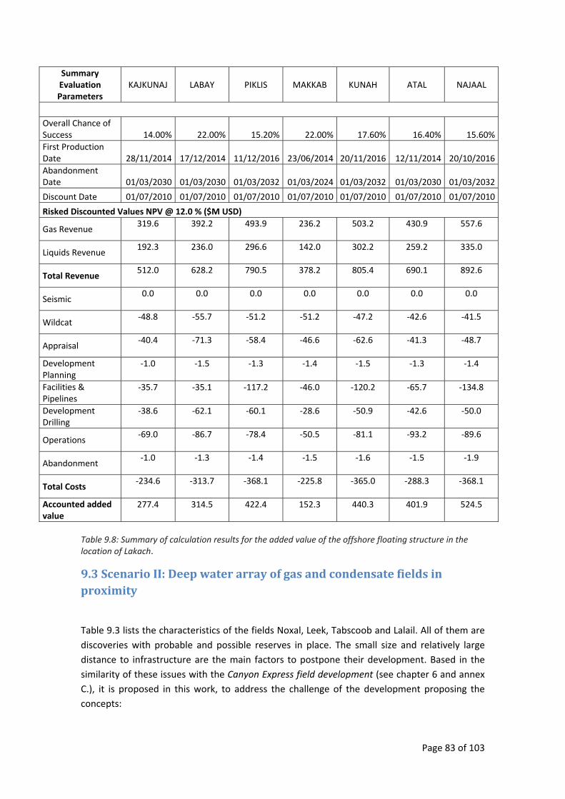
Page 83 of 103
Summary Evaluation Parameters
KAJKUNAJ LABAY PIKLIS MAKKAB KUNAH ATAL NAJAAL
Overall Chance of Success 14.00% 22.00% 15.20% 22.00% 17.60% 16.40% 15.60%First Production Date 28/11/2014 17/12/2014 11/12/2016 23/06/2014 20/11/2016 12/11/2014 20/10/2016Abandonment Date 01/03/2030 01/03/2030 01/03/2032 01/03/2024 01/03/2032 01/03/2030 01/03/2032
Discount Date 01/07/2010 01/07/2010 01/07/2010 01/07/2010 01/07/2010 01/07/2010 01/07/2010
Risked Discounted Values NPV @ 12.0 % ($M USD)
Gas Revenue 319.6 392.2 493.9 236.2 503.2 430.9 557.6
Liquids Revenue 192.3 236.0 296.6 142.0 302.2 259.2 335.0
Total Revenue 512.0 628.2 790.5 378.2 805.4 690.1 892.6
Seismic 0.0 0.0 0.0 0.0 0.0 0.0 0.0
Wildcat ‐48.8 ‐55.7 ‐51.2 ‐51.2 ‐47.2 ‐42.6 ‐41.5
Appraisal ‐40.4 ‐71.3 ‐58.4 ‐46.6 ‐62.6 ‐41.3 ‐48.7
Development Planning
‐1.0 ‐1.5 ‐1.3 ‐1.4 ‐1.5 ‐1.3 ‐1.4
Facilities & Pipelines
‐35.7 ‐35.1 ‐117.2 ‐46.0 ‐120.2 ‐65.7 ‐134.8
Development Drilling
‐38.6 ‐62.1 ‐60.1 ‐28.6 ‐50.9 ‐42.6 ‐50.0
Operations ‐69.0 ‐86.7 ‐78.4 ‐50.5 ‐81.1 ‐93.2 ‐89.6
Abandonment ‐1.0 ‐1.3 ‐1.4 ‐1.5 ‐1.6 ‐1.5 ‐1.9
Total Costs ‐234.6 ‐313.7 ‐368.1 ‐225.8 ‐365.0 ‐288.3 ‐368.1
Accounted added value
277.4 314.5 422.4 152.3 440.3 401.9 524.5
Table 9.8: Summary of calculation results for the added value of the offshore floating structure in the location of Lakach.
9.3 Scenario II: Deep water array of gas and condensate fields in proximity
Table 9.3 lists the characteristics of the fields Noxal, Leek, Tabscoob and Lalail. All of them are discoveries with probable and possible reserves in place. The small size and relatively large distance to infrastructure are the main factors to postpone their development. Based in the similarity of these issues with the Canyon Express field development (see chapter 6 and annex C.), it is proposed in this work, to address the challenge of the development proposing the concepts:
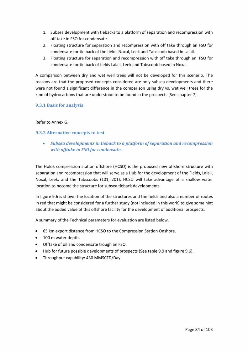
Page 84 of 103
1. Subsea development with tiebacks to a platform of separation and recompression with off take in FSO for condensate.
2. Floating structure for separation and recompression with off take through an FSO for condensate for tie back of the fields Noxal, Leek and Tabscoob based in Lalail.
3. Floating structure for separation and recompression with off take through an FSO for condensate for tie back of fields Lalail, Leek and Tabscoob based in Noxal.
A comparison between dry and wet well trees will not be developed for this scenario. The reasons are that the proposed concepts considered are only subsea developments and there were not found a significant difference in the comparison using dry vs. wet well trees for the kind of hydrocarbons that are understood to be found in the prospects (See chapter 7).
9.3.1 Basis for analysis
Refer to Annex G.
9.3.2 Alternative concepts to test
• Subsea developments in tieback to a platform of separation and recompression with offtake in FSO for condensate.
The Holok compression station offshore (HCSO) is the proposed new offshore structure with separation and recompression that will serve as a Hub for the development of the Fields, Lalail, Noxal, Leek, and the Tabscoobs (101, 201). HCSO will take advantage of a shallow water location to become the structure for subsea tieback developments.
In figure 9.6 is shown the location of the structures and the fields and also a number of routes in red that might be considered for a further study (not included in this work) to give some hint about the added value of this offshore facility for the development of additional prospects.
A summary of the Technical parameters for evaluation are listed below.
• 65 km export distance from HCSO to the Compression Station Onshore.
• 100 m water depth.
• Offtake of oil and condensate trough an FSO.
• Hub for future possible developments of prospects (See table 9.9 and figure 9.6).
• Throughput capability: 430 MMSCFD/Day
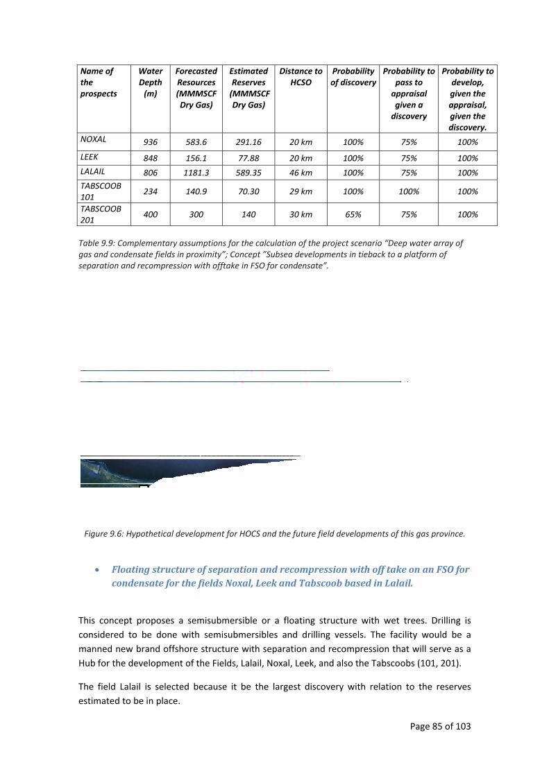
Page 85 of 103
Name of the prospects
Water Depth (m)
Forecasted Resources (MMMSCF Dry Gas)
Estimated Reserves (MMMSCF Dry Gas)
Distance to HCSO
Probability of discovery
Probability to pass to appraisal given a discovery
Probability to develop, given the appraisal, given the discovery.
NOXAL 936 583.6 291.16 20 km 100% 75% 100%
LEEK 848 156.1 77.88 20 km 100% 75% 100% LALAIL 806 1181.3 589.35 46 km 100% 75% 100% TABSCOOB 101
234 140.9 70.30 29 km 100% 100% 100%
TABSCOOB 201
400 300 140 30 km 65% 75% 100%
Table 9.9: Complementary assumptions for the calculation of the project scenario “Deep water array of gas and condensate fields in proximity”; Concept ”Subsea developments in tieback to a platform of separation and recompression with offtake in FSO for condensate”.
Figure 9.6: Hypothetical development for HOCS and the future field developments of this gas province.
• Floating structure of separation and recompression with off take on an FSO for condensate for the fields Noxal, Leek and Tabscoob based in Lalail.
This concept proposes a semisubmersible or a floating structure with wet trees. Drilling is considered to be done with semisubmersibles and drilling vessels. The facility would be a manned new brand offshore structure with separation and recompression that will serve as a Hub for the development of the Fields, Lalail, Noxal, Leek, and also the Tabscoobs (101, 201).
The field Lalail is selected because it be the largest discovery with relation to the reserves estimated to be in place.

Page 86 of 103
Figure 9.7 shows the relative location of the fields and also a number of routes in red that might be considered for a further study (not included in this work) to give more basis to estimate the added value of this offshore facility for the development of additional prospects.
A summary of the Technical parameters for evaluation are listed below.
• 110 km Export distance from the Lalail floating hub to the Compression Station Onshore.
• 806 m water depth.
• Offtake of oil and condensate trough an FSO.
• Hub for future possible developments of prospects (See table 9.10 and figure 9.7).
• Throughput capability: 430 MMSCFD/Day
Name of the prospects
Water Depth (m)
Forecasted Resources (MMMSCF Dry Gas)
Estimated Reserves (MMMSCF Dry Gas)
Distance to LALAIL
Probability of discovery
Probability to pass to appraisal given a discovery
Probability to develop, given the appraisal, given the discovery.
LALAIL 806 1181.3 589.35 ‐‐‐‐‐‐‐‐‐‐‐ 100% 75% 100% NOXAL 936 583.6 291.16 5 km 100% 75% 100%
LEEK 848 156.1 77.88 30 km5 100% 75% 100% TABSCOOB 201
400 300 140 17 km 65% 75% 100%
TABSCOOB 101
234 140.9 70.30 7 km6 100% 100% 100%
Table 9.10: Complementary assumptions for the calculation of the project scenario “Deep water array of gas and condensate fields in proximity”; Concept ” Floating structure of separation and recompression with off take in FSO for condensate for the fields Noxal, Leek and Tabscoob based in Lalail”.
Figure 9.7: Hypothetical development for a Floating structure in Lalail also as a Hub for the future field developments of this gas province. 5 Note: A daisy chain Noxal‐Leek_Lalailwill be evaluated 6 Note: A daisy chain Lalail ‐ Tabscoob (101) – Tabscoob (201) will be evaluated.
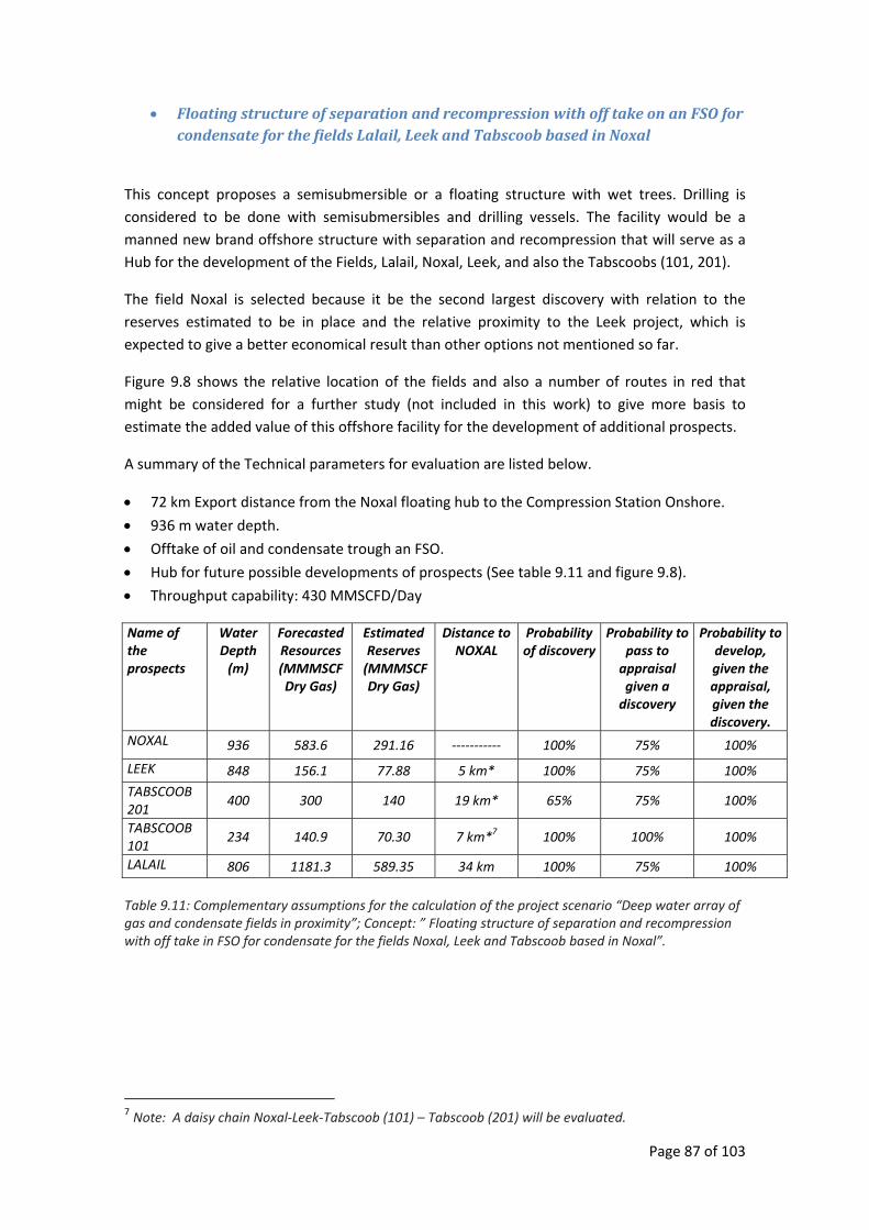
Page 87 of 103
• Floating structure of separation and recompression with off take on an FSO for condensate for the fields Lalail, Leek and Tabscoob based in Noxal
This concept proposes a semisubmersible or a floating structure with wet trees. Drilling is considered to be done with semisubmersibles and drilling vessels. The facility would be a manned new brand offshore structure with separation and recompression that will serve as a Hub for the development of the Fields, Lalail, Noxal, Leek, and also the Tabscoobs (101, 201).
The field Noxal is selected because it be the second largest discovery with relation to the reserves estimated to be in place and the relative proximity to the Leek project, which is expected to give a better economical result than other options not mentioned so far.
Figure 9.8 shows the relative location of the fields and also a number of routes in red that might be considered for a further study (not included in this work) to give more basis to estimate the added value of this offshore facility for the development of additional prospects.
A summary of the Technical parameters for evaluation are listed below.
• 72 km Export distance from the Noxal floating hub to the Compression Station Onshore.
• 936 m water depth.
• Offtake of oil and condensate trough an FSO.
• Hub for future possible developments of prospects (See table 9.11 and figure 9.8).
• Throughput capability: 430 MMSCFD/Day
Name of the prospects
Water Depth (m)
Forecasted Resources (MMMSCF Dry Gas)
Estimated Reserves (MMMSCF Dry Gas)
Distance to NOXAL
Probability of discovery
Probability to pass to appraisal given a discovery
Probability to develop, given the appraisal, given the discovery.
NOXAL 936 583.6 291.16 ‐‐‐‐‐‐‐‐‐‐‐ 100% 75% 100%
LEEK 848 156.1 77.88 5 km* 100% 75% 100% TABSCOOB 201
400 300 140 19 km* 65% 75% 100%
TABSCOOB 101
234 140.9 70.30 7 km*7 100% 100% 100%
LALAIL 806 1181.3 589.35 34 km 100% 75% 100% Table 9.11: Complementary assumptions for the calculation of the project scenario “Deep water array of gas and condensate fields in proximity”; Concept: ” Floating structure of separation and recompression with off take in FSO for condensate for the fields Noxal, Leek and Tabscoob based in Noxal”.
7 Note: A daisy chain Noxal‐Leek‐Tabscoob (101) – Tabscoob (201) will be evaluated.
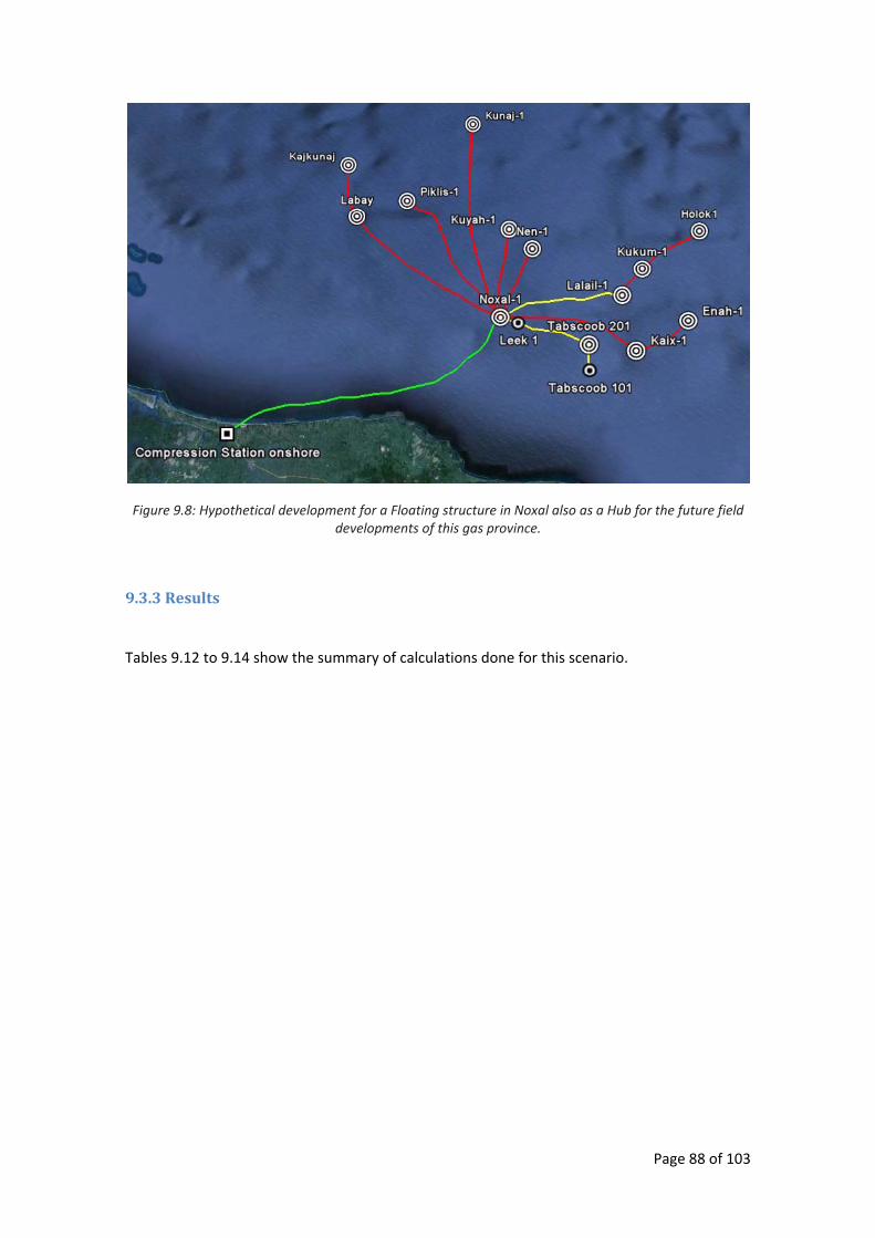
Page 88 of 103
Figure 9.8: Hypothetical development for a Floating structure in Noxal also as a Hub for the future field developments of this gas province.
9.3.3 Results
Tables 9.12 to 9.14 show the summary of calculations done for this scenario.
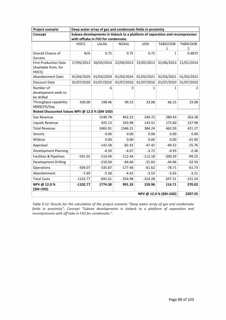
Page 89 of 103
Project scenario Deep water array of gas and condensate fields in proximity Concept Subsea developments in tieback to a platform of separation and recompression
with offtake in FSO for condensate. HOCS LALAIL NOXAL LEEK TABSCOOB
1 TABSCOOB
2 Overall Chance of Success
N/A 0.75 0.75 0.75 1 0.4875
First Production Date (Available from, for HOCS)
17/05/2012 26/03/2014 22/09/2013 25/05/2013 01/06/2013 21/01/2014
Abandonment Date 01/04/2029 01/03/2029 01/03/2024 01/03/2021 01/03/2021 01/03/2022
Discount Date 01/07/2010 01/07/2010 01/07/2010 01/07/2010 01/07/2010 01/07/2010
Number of development wells to be drilled
6 3 1 1 2
Throughput capability: MMSCFD/Day
430.00 198.46 99.23 33.08 66.15 33.08
Risked Discounted Values NPV @ 12.0 % ($M USD)
Gas Revenue 1540.78 842.32 240.72 289.43 263.28
Liquids Revenue 925.13 503.98 143.52 172.60 157.98
Total Revenue 2465.91 1346.31 384.24 462.03 421.27
Seismic 0.00 0.00 0.00 0.00 0.00
Wildcat 0.00 0.00 0.00 0.00 ‐41.90
Appraisal ‐142.58 ‐82.43 ‐47.42 ‐49.52 ‐25.76
Development Planning ‐4.50 ‐4.07 ‐3.72 ‐4.93 ‐2.36
Facilities & Pipelines ‐591.01 ‐214.04 ‐112.44 ‐113.18 ‐200.39 ‐99.25
Development Drilling ‐210.04 ‐84.66 ‐31.64 ‐44.96 ‐32.59
Operations ‐504.07 ‐335.87 ‐177.46 ‐61.62 ‐78.71 ‐61.73
Abandonment ‐7.69 ‐5.58 ‐4.42 ‐3.53 ‐5.63 ‐3.21
Total Costs ‐1102.77 ‐691.61 ‐354.98 ‐224.28 ‐347.31 ‐151.24
NPV @ 12.0 % ($M USD)
‐1102.77 1774.30 991.33 159.96 114.71 270.02
NPV @ 12.0 % ($M USD) 2207.55
Table 9.12: Results for the calculation of the project scenario “Deep water array of gas and condensate fields in proximity”; Concept ”Subsea developments in tieback to a platform of separation and recompression with off take in FSO for condensate.”.
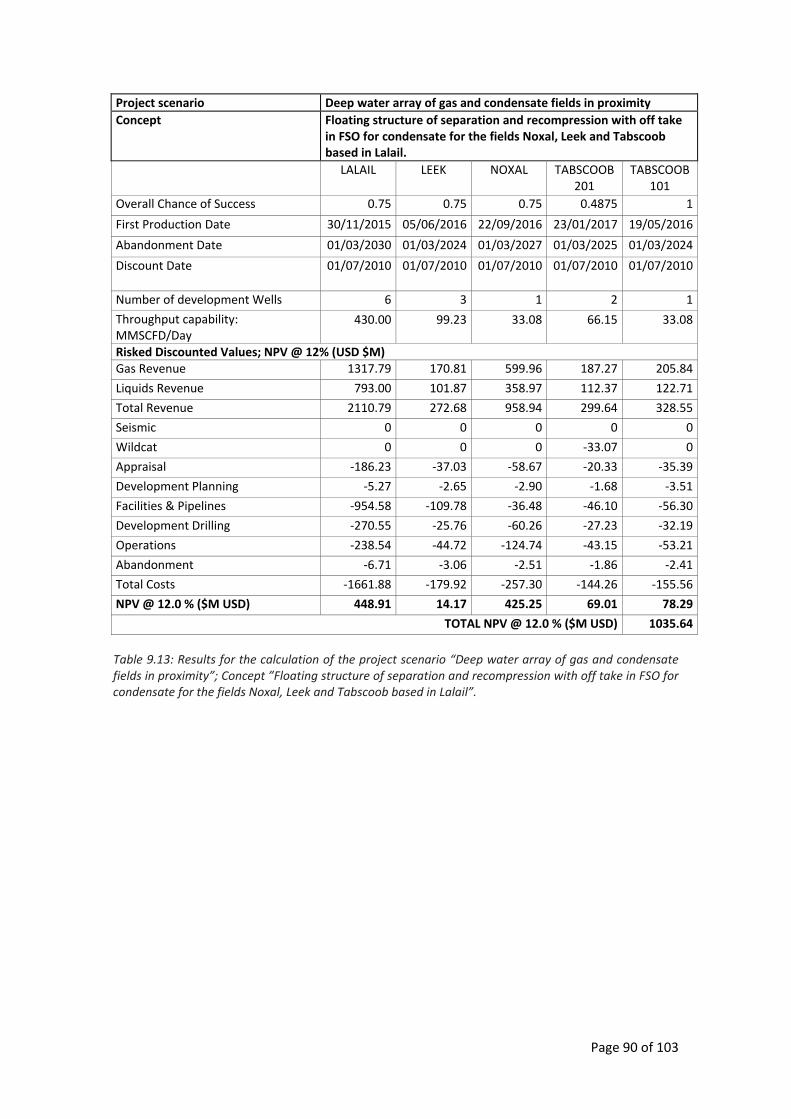
Page 90 of 103
Project scenario Deep water array of gas and condensate fields in proximity Concept Floating structure of separation and recompression with off take
in FSO for condensate for the fields Noxal, Leek and Tabscoob based in Lalail.
LALAIL LEEK NOXAL TABSCOOB 201
TABSCOOB 101
Overall Chance of Success 0.75 0.75 0.75 0.4875 1
First Production Date 30/11/2015 05/06/2016 22/09/2016 23/01/2017 19/05/2016
Abandonment Date 01/03/2030 01/03/2024 01/03/2027 01/03/2025 01/03/2024
Discount Date 01/07/2010 01/07/2010 01/07/2010 01/07/2010 01/07/2010
Number of development Wells 6 3 1 2 1
Throughput capability: MMSCFD/Day
430.00 99.23 33.08 66.15 33.08
Risked Discounted Values; NPV @ 12% (USD $M)Gas Revenue 1317.79 170.81 599.96 187.27 205.84
Liquids Revenue 793.00 101.87 358.97 112.37 122.71
Total Revenue 2110.79 272.68 958.94 299.64 328.55
Seismic 0 0 0 0 0
Wildcat 0 0 0 ‐33.07 0
Appraisal ‐186.23 ‐37.03 ‐58.67 ‐20.33 ‐35.39
Development Planning ‐5.27 ‐2.65 ‐2.90 ‐1.68 ‐3.51
Facilities & Pipelines ‐954.58 ‐109.78 ‐36.48 ‐46.10 ‐56.30
Development Drilling ‐270.55 ‐25.76 ‐60.26 ‐27.23 ‐32.19
Operations ‐238.54 ‐44.72 ‐124.74 ‐43.15 ‐53.21
Abandonment ‐6.71 ‐3.06 ‐2.51 ‐1.86 ‐2.41
Total Costs ‐1661.88 ‐179.92 ‐257.30 ‐144.26 ‐155.56
NPV @ 12.0 % ($M USD) 448.91 14.17 425.25 69.01 78.29
TOTAL NPV @ 12.0 % ($M USD) 1035.64
Table 9.13: Results for the calculation of the project scenario “Deep water array of gas and condensate fields in proximity”; Concept ”Floating structure of separation and recompression with off take in FSO for condensate for the fields Noxal, Leek and Tabscoob based in Lalail”.
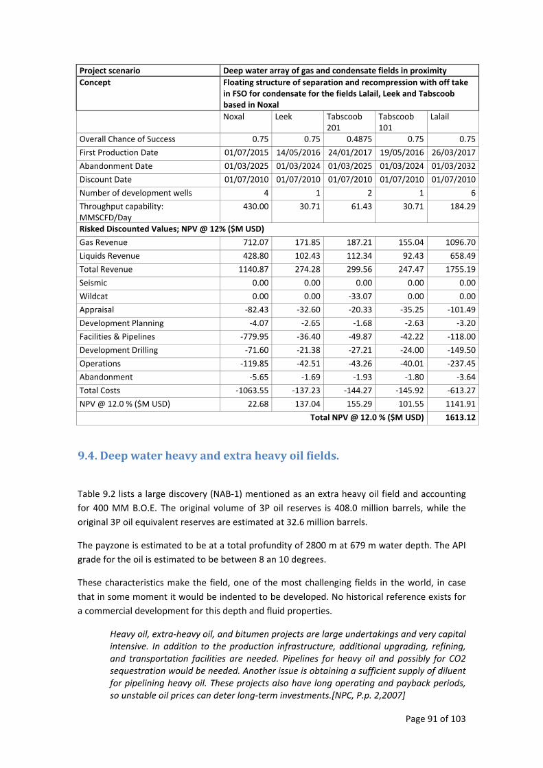
Page 91 of 103
Project scenario Deep water array of gas and condensate fields in proximity Concept Floating structure of separation and recompression with off take
in FSO for condensate for the fields Lalail, Leek and Tabscoob based in Noxal
Noxal Leek Tabscoob 201
Tabscoob 101
Lalail
Overall Chance of Success 0.75 0.75 0.4875 0.75 0.75
First Production Date 01/07/2015 14/05/2016 24/01/2017 19/05/2016 26/03/2017
Abandonment Date 01/03/2025 01/03/2024 01/03/2025 01/03/2024 01/03/2032
Discount Date 01/07/2010 01/07/2010 01/07/2010 01/07/2010 01/07/2010
Number of development wells 4 1 2 1 6
Throughput capability: MMSCFD/Day
430.00 30.71 61.43 30.71 184.29
Risked Discounted Values; NPV @ 12% ($M USD)
Gas Revenue 712.07 171.85 187.21 155.04 1096.70
Liquids Revenue 428.80 102.43 112.34 92.43 658.49
Total Revenue 1140.87 274.28 299.56 247.47 1755.19
Seismic 0.00 0.00 0.00 0.00 0.00
Wildcat 0.00 0.00 ‐33.07 0.00 0.00
Appraisal ‐82.43 ‐32.60 ‐20.33 ‐35.25 ‐101.49
Development Planning ‐4.07 ‐2.65 ‐1.68 ‐2.63 ‐3.20
Facilities & Pipelines ‐779.95 ‐36.40 ‐49.87 ‐42.22 ‐118.00
Development Drilling ‐71.60 ‐21.38 ‐27.21 ‐24.00 ‐149.50
Operations ‐119.85 ‐42.51 ‐43.26 ‐40.01 ‐237.45
Abandonment ‐5.65 ‐1.69 ‐1.93 ‐1.80 ‐3.64
Total Costs ‐1063.55 ‐137.23 ‐144.27 ‐145.92 ‐613.27
NPV @ 12.0 % ($M USD) 22.68 137.04 155.29 101.55 1141.91
Total NPV @ 12.0 % ($M USD) 1613.12
9.4. Deep water heavy and extra heavy oil fields.
Table 9.2 lists a large discovery (NAB‐1) mentioned as an extra heavy oil field and accounting for 400 MM B.O.E. The original volume of 3P oil reserves is 408.0 million barrels, while the original 3P oil equivalent reserves are estimated at 32.6 million barrels.
The payzone is estimated to be at a total profundity of 2800 m at 679 m water depth. The API grade for the oil is estimated to be between 8 an 10 degrees.
These characteristics make the field, one of the most challenging fields in the world, in case that in some moment it would be indented to be developed. No historical reference exists for a commercial development for this depth and fluid properties.
Heavy oil, extra‐heavy oil, and bitumen projects are large undertakings and very capital intensive. In addition to the production infrastructure, additional upgrading, refining, and transportation facilities are needed. Pipelines for heavy oil and possibly for CO2 sequestration would be needed. Another issue is obtaining a sufficient supply of diluent for pipelining heavy oil. These projects also have long operating and payback periods, so unstable oil prices can deter long‐term investments.[NPC, P.p. 2,2007]
Page 92 of 103
Additional information on this respect might be consulted in “Topic paper #22, heavy oil” (NPC, 2007).
9.5. Conclusions
In the first scenario, it was found that the best Net Present Value assessment result for the development of the Lakach field is the concept of subsea tieback to shore. This is true when an additional value for the development of infrastructure in the region is not considered. Although the concept has higher economical penalties in the RAMEX because of the higher costs for it maintenance, the savings in the CAPEX are notorious.
On the other hand, the potential of the Region of Holok‐Temoa, related to the prospects listed in table 9.4, might increase considerably the strategic value of the investments in infrastructure. This infrastructure would be available when offshore structures and a network of pipelines will be developed in the region.
Lakach development has an ample positive Net Present Value before taxes even when a floating structure was selected. Also the calculated added value that could be obtained by using the floating structure as a hub as shown in table 9.8. Lakach has also a geographical advantage since it is located at less than 1000 meters of water depth; much easier to develop when is compared to other identified prospects of development that go from 1700 m up to 2500 m water depth.
Figure 9.5 shows a hypothetical development that could have Lakach as a processing Hub for the future field developments of this gas province.
The Lakach Field development has already been committed to be developed as a subsea tieback to shore. Consequently for future concept selection, it is strongly recommended to keep in mind the fact that the development of infrastructure increases the feasibility of future developments and increase the overall recoveries rates from the oil and gas fields.
On the second scenario, It was found that a series of medium‐small size fields might be economically developed when they are planned as a group of fields.
The best NPV concept assessed for this scenario was a “Subsea development with tiebacks to a platform of separation and recompression with off take on an FSO for condensate”, meanwhile the higher investment costs for floating structures either in Lalail or Noxal make them not a sounded option for efficient investment of resources.
A platform for separation and recompression, here named as “The Holok compression station offshore (HCSO)” is a proposed new brand offshore structure with separation and recompression that will serve as a Hub for the development of the Fields, Lalail, Noxal, Leek, and the Tabscoobs (101, 201). HCSO will take advantage of a shallow water location to become the structure for subsea tieback developments.
Page 93 of 103
This proposed structure will reduce the costs of the development and at the same time become a high added value for future developments since its reach is comparatively equivalent with floating structures located in the Lalal and Noxal sites.
An additional advantage for the Mexican Industry as a whole is that these kind of shallow water facilities are in the scope of the capability of national contractors. This is a high potential argument on behalf of the national content that PEMEX can encourage through its corporate decisions.
Regarding the heavy and extra heavy oil discoveries, the opinion of this author is that the Exploration activities in deep water should be focused on prospects potentially commercial instead of looking for resources that can barely be produced (API‐15 or less). Although the diversification of opportunities for exploration should be encouraged, is the opinion of this author that it should be focused on the Region of Holok Temoa or others that could have a similar potential of development in the short term.
There is no doubt that additional discoveries in the Holok Temoa Integral Asset and in general in the deep water in Mexico will be made in the future, but there are some few recommendations that could be issued after the development of this study.
1. It is suggested to design, coordinate and follow a strategic plan for field development in all the regions in the domain of PEMEX, looking for maximizing the possibilities of development and ensure efficient depletion of the natural resources located in Mexican territorial waters.
2. Encourage the investments in infrastructure since it makes feasible future field development and increase the capability of efficient depletion.
3. Encourage solutions that will make possible a gradual assimilation of technology for both the National Oil Company and for the national contractors. The economically feasible solutions that open the participation of national suppliers alone or in association with international contractors should have extra points in the formal assessment of concepts.
4. Exploration and appraisal should focus on prospects that are commercial in the short run. The drilling in deep water is not only expensive but it could be notoriously ineffective if it is not linked to the value chain of potential field developments.
Page 94 of 103
10. General Conclusions
10.1 On the discussion on the recovery factor Dry vs. Wet Tree
In order to give validity to the model of LCC analysis here proposed, an empirical comparison on the resulting recovery factor based on data of the US Gulf of Mexico was included in the scope of this work. This comparison was intended to answer ¿Is there a significant difference in the recovery factor when is used the dry tree vs. the wet tree concept solutions?
The oil and gas recovery factors listed in this data set analyzed correspond to the estimated values declared by the operator companies to the MMS for sands located in the US Gulf of Mexico. The values are subject to change due to different factors including technology improvements, operations management philosophy and refinement of calculations as more information from the reservoirs become available
The class of fields most exploited in deepwater in Gulf of Mexico corresponds to undersaturated oil fields (≈ 65%) followed by the non associated class (≈ 30%) and finally saturated oil fields class (≈ 4%).
The mean recovery factors for the different types of reservoir are summarized in table 7.5.
According to the test of hypothesis mdry tree‐ mwet tree = 0 vs. mdry tree‐ mwet tree ≠ 0 with m
calculated from the data sets created in this methodology, there is not statistical evidence that suggest that a field developed with dry tree has a better recovery factor than one developed with wet tree solutions.
With exception of the gas recovery factor from saturated oil fields, all the other test fail to
reject the null hypothesis mdry tree‐ mwet tree = 0. This means that the inferred mean value of
recovery factor is the same either for dry tree vs wet tree solutions.
In the only exception (gas recovery factor of the saturated oil fields) is perceptibly a difference in favor of the dry tree. Despite the oil recovery factor from the same type of reservoirs is larger for dry tree than for the wet tree, the pooled variance for both samples is too large to make a differentiation on their means.
It is inferred that a criteria that prefer a dry tree with the argument of a better recovery factor must be evaluated further, extending the analysis to consider the specific characteristics of the reservoir and the exploitation concept that is part of the field to be developed.
Consecuently a model that include a reservoir complexity index was presented and analized. The Reservoir Complexity Index from the Norwegian petroleum directorate on the performance of dry and wet tree solutions was discussed.
From a presentation provided by the NPD a data set was extracted for fields encompassed by an study differentiating the dry tree and the wet tree developments. The results of the analysis of this data set are shown graphically in figure 7.2.
Page 95 of 103
What can be inferred from the figure 7.2 is that on the Norwegian Continental Shelf, depending of the complexity of the reservoir, there is:
A linear trend on the recovery factor for fields developed with dry tree to decrease as the reservoir becomes more complex.
An exponential trend on the recovery factor for fields developed with wet tree to decrease as the reservoir becomes more complex. A linear trend was also tested but is not shown because the exponential regressed function has a better R2 (R2 = 0.5891 in linear regression vs R2 = 0.6672 in exponential regression).
When the reservoir has a low complexity (up to 0.4) it seems that there is not an evident difference between the performances of dry vs wet tree solutions. As the complexity increases however the dry tree solutions become a better option based on the recovery factor registered.
Many oil companies worldwide employ methodologies similar to the RCI as a common basis. Although the calculation of this index is out of the scope of this work it could be useful for the reader to take a look on the patented work of Harrison (Harrison, 2004) who propose “A method for computing complexity, confidence and technical maturity indices for the evaluation of a reservoir.”
10.2 On the Case Analysis
Two hypothetical projects (three different concepts for each project) of field development, based in public information released by PEMEX, are assessed.
Scenario I: Deep water stand alone gas field
• Concepts: Subsea Tieback to Shore; TLP with dry tree, export pipeline for gas and off take through FSO for condensate; SPAR with dry tree, export pipeline for gas and off take through FSO for condensate.
Scenario II: Deep water array of gas and condensate fields in proximity
• Concepts: Subsea development with tiebacks to a platform of separation and recompression with off take in FSO for condensate; Floating structure for separation and recompression with off take through an FSO for condensate for tie back of the fields Noxal, Leek and Tabscoob based in Lalail; Floating structure for separation and recompression with off take through an FSO for condensate for tie back of fields Lalail, Leek and Tabscoob based in Noxal.
In the first scenario, it was found that the best Net Present Value assessment result for the development of the Lakach field is the concept of subsea tieback to shore. This is true when an additional value for the development of infrastructure in the region is not considered. Although the concept has higher economical penalties in the RAMEX because of the higher costs for it maintenance, the savings in the CAPEX are notorious.
Page 96 of 103
On the other hand, the potential of the Region of Holok‐Temoa, related to the prospects listed in table 9.4, might increase considerably the strategic value of the investments in infrastructure. This infrastructure would be available when offshore structures and a network of pipelines will be developed in the region.
Lakach development has an ample positive Net Present Value before taxes even when a floating structure was selected. Also the calculated added value that could be obtained by using the floating structure as a hub as shown in table 9.8. Lakach has also a geographical advantage since it is located at less than 1000 meters of water depth; much easier to develop when is compared to other identified prospects of development that go from 1700 m up to 2500 m water depth.
Figure 9.5 shows a hypothetical development that could have Lakach as a processing Hub for the future field developments of this gas province.
The Lakach Field development has already been committed to be developed as a subsea tieback to shore. Consequently for future concept selection, it is strongly recommended to keep in mind the fact that the development of infrastructure increases the feasibility of future developments and increase the overall recoveries rates from the oil and gas fields.
On the second scenario, It was found that a series of medium‐small size fields might be economically developed when they are planned as a group of fields.
The best NPV concept assessed for this scenario was a “Subsea development with tiebacks to a platform of separation and recompression with off take on an FSO for condensate”, meanwhile the higher investment costs for floating structures either in Lalail or Noxal make them not a sounded option for efficient investment of resources.
A platform for separation and recompression, here named as “The Holok compression station offshore (HCSO)” is a proposed new brand offshore structure with separation and recompression that will serve as a Hub for the development of the Fields, Lalail, Noxal, Leek, and the Tabscoobs (101, 201). HCSO will take advantage of a shallow water location to become the structure for subsea tieback developments.
This proposed structure will reduce the costs of the development and at the same time become a high added value for future developments since its reach is comparatively equivalent with floating structures located in the Lalal and Noxal sites.
An additional advantage for the Mexican Industry as a whole is that these kind of shallow water facilities are in the scope of the capability of national contractors. This is a high potential argument on behalf of the national content that PEMEX can encourage through its corporate decisions.
Regarding the heavy and extra heavy oil discoveries, the opinion of this author is that the Exploration activities in deep water should be focused on prospects potentially commercial instead of looking for resources that can barely be produced (API‐15 or less). Although the diversification of opportunities for exploration should be encouraged, is the opinion of this
Page 97 of 103
author that it should be focused on the Region of Holok Temoa or others that could have a similar potential of development in the short term.
10.3 Recommendations
There is no doubt that additional discoveries in the Holok Temoa Integral Asset and in general in the deep water in Mexico will be made in the future, but there are some few recommendations that could be issued after the development of this study.
1. It is suggested to design, coordinate and follow a strategic plan for field development in all the regions in the domain of PEMEX, looking for maximizing the possibilities of development and ensure efficient depletion of the natural resources located in Mexican territorial waters.
2. Encourage the investments in infrastructure since it makes feasible future field development and increase the capability of efficient depletion.
3. Encourage solutions that will make possible a gradual assimilation of technology for both the National Oil Company and for the national contractors. The economically feasible solutions that open the participation of national suppliers alone or in association with international contractors should have extra points in the formal assessment of concepts.
4. Exploration and appraisal should focus on prospects that are commercial in the short run. The drilling in deep water is not only expensive but it could be notoriously ineffective if it is not linked to the value chain of potential field developments.
Page 98 of 103
References
1. Adams N. “Introduction to well planning”, Petroleum Engineering Handbook, Edited by Lake W., Volume II Drilling Engineering, Edited by Mitchell R.F., Society of Petroleum Engineering, 2006.
2. American National Standards Institute/ American Petroleum Institute, (ANSI/API), “Recommended Practice for Planning, Designing and Constructing Tension Leg Platforms” Second Edition, August, 1997
3. American Petroleum Institute, (API), “Interim Guidance on Hurricane Conditions in the Gulf of Mexico”, Bulletin 2INT‐MET, USA, 2007.
1. American Petroleum Institute, (API), “Recommended Practice for Subsea Production System Reliability and Technical Risk Management” API recommended practice 17N, first edition, March 2009.
4. Babusiaux D., Favennec J., Bauquis P., Bret‐Rouzaut N. and Guirauden D. “Oil and gas exploration and production : reserves, costs, contracts”; translated by Pears J.. Ed. Technip, Institut Français du petrole, Paris, France, 2004.
5. Ball I.G. Subsea Domain Ltg, “Challenges of long satellite tiebacks” Paper OTC 18405, Offshore Technology Conference, USA, 2006.
6. Bass R.M., Shell Intl. E&P “Subsea Processing and Boosting—Technical Challenges and Opportunities”, Paper OTC 18621, Offshore Technology Conference, 2006.
7. Brandt H., Det Norske Veritas (U.S.A.), Inc. “Risk comparison subsea vs. surface processing” Final Report Submitted to the U.S. Department of Interior – Minerals Management Service (MMS), Technology Assessment & Research (TA&R) Program Project Number: 500, Texas, USA, December 15, 2004.
8. Bygdevoll J. “Introduction to Reservoir Complextiy Index (RCI)” Lecture by the
Norwegian Petroleum Directorate, 18.03.2010.
9. Capanoglu C. I.D.E.A.S. Inc. San Francisco CA. USA, “Novel and Marginal Offshore Structures” Handbook of Offshore Engineering Edited by Chakrabarti S., USA. 2005.
10. Coker J.W.A. and Gudmestad O.T. Statoil “Introduction to development of a petroleum installation”, Norwegian Agency for Development and Cooperation (NORAD), Oil for Development Information Package, Resource Management, Development and Operation , Additional Literature, Stavanger, Norway, 2003. Available at internet: http://www.norad.no/en/Thematic+areas/Energy/Oil+for+Development/OfD+Information+Package/Resource+Management Last visited April 19th, 2010.
11. Chakrabarti S. Offshore structure analysis Inc. Plainfield, IL, USA, Capanoglu C. I.D.E.A.S. Inc. San Francisco CA. USA, Halkyard J. Technip Offshore, Inc. Houston TX,
Page 99 of 103
USA. “Historical development of offshore structures” Handbook of Offshore Engineering Edited by Chakrabarti S., USA. 2005.
12. Childers M.A. “Offshore drilling units”, Petroleum Engineering Handbook, Edited by Lake W., Volume II Drilling Engineering, Edited by Mitchell R.F., Society of Petroleum Engineering, 2006.
13. Craig Jr. F.F. “Reservoir Engineering Aspects Of Waterflooding”, Society of Petroleum Engineers, 1993.
14. FMC, FMC technologies, “Subsea Processing Boosting”. Available at internet: http://www.fmctechnologies.com/SubseaSystems/Technologies/AdvancingTechnologies/SubseaProcessingBoosting.aspx, last visited 28 August 2009.
15. Goldsmith R., Goldsmith Engineering, Inc. Eriksen R. and Childs M., Det Norske Veritas, Inc. Saucier B. , Subsea Consultant, Deegan F.J., Vectra Technologies, Ltd. “Lifetime Cost of Subsea Production Systems, prepared for Subsea JIP, System Description & FMEA” Project Report Prepared for the Minerals Management Service MMS Project Number 331, Rev. 2, June, 2000.
16. Green D.W., Willihite G.P. “Enhanced Oil Recovery”, Society of Petroleum Engineers, 1998.
17. Harrel R. and Cronquist C. “Estimation of primary reserves of crude oil, natural gas, and condensates”, Petroleum Engineering Handbook, Edited by LakeW. Volume V Reservoir Engineering and Petrophysics, Edited by Holstein. E.D., Society of Petroleum Engineering, 2007.
18. Harrison C.J. Chevron U.S.A. Inc. “Method for computing complexity, confidence and technical maturity indices for reservoir evaluations” United States Patent 6810332, 2004.
19. Halkyard J. Technip Offshore, Inc. Houston TX, USA., Filson J. Gig Harbor , WA, USA., Thiagarajan K. The University of Western Australia, Perth, Australia. “Floating offshore platform design” Handbook of Offshore Engineering Edited by Chakrabarti S., USA. 2005.
20. Hernández G. PEP, PEMEX Exploracion y Producción, “Presente y futuro de las estrategias de exploración y explotación en aguas profundas” Foro Retos tecnológicos para la exploración y explotación en aguas profundas, Comisión de Especialidad de Ingeniería Petrolera de la Academia de Ingeniería A.C. , Octubre 15‐16, 2009. Available at Internet: http://www.ai.org.mx/archivos/foros/aguas‐profundas/PEP%20Foro%20Discusion%201.pdf last consulted May 1st, 2010.
21. HIS Indexes, “IHS CERA Upstream Capital Costs Index (UCCI)” IHS Inc., U.S.A., 2010 Available at internet http://www.ihsindexes.com/index.htm, last visited 29th May, 2010.
Page 100 of 103
22. Håvard D. “Oil and gas production handbook, an Introduction to oil and gas
production” ABB ATPA Oil and Gas, Oslo, Norway, 2006.
23. International Standard Organization (ISO), “ISO‐13628‐1:2005, Petroleum and natural gas industries — Design and operation of subsea production systems — Part 1: General requirements and recommendations”, Switzerland, 2005.
24. International Standard Organization (ISO), “IS0‐19904‐1:2006, Petroleum and natural gas industries — Floating offshore structures Part 1: Monohulls, semi‐submersibles and spars”, Switzerland, 2006.
25. Jablanowski C.,The University of Texas at Austin, Strachan A., Wood Mackenzie “Empirical cost models for TLPs and Spars ”, Paper SPE 115483, Society of Petroleum Engineers, 2008.
26. Kaiser M. and Pulsipher A. “Fiscal System Analysis: Concessionary and Contractual Systems used in Offshore Petroleum Arrangements” Prepared under MMS Contract 1435‐01‐01‐30951‐18178 by Center for Energy Studies, Louisiana State University, Baton Rouge, Louisiana, U.S.A. 2004.
27. Karsan D. Paragon Engineering Services Inc. Houston, TX, USA, Rammohan V. Stress Offshore Inc. Houston TX. USA. “Fixed offshore platform design” Handbook of Offshore Engineering Edited by Chakrabarti S., USA. 2005.
28. Kibbee S.E., Snell D.C., Atlantia Offshore Limited, Member of the IHC Caland Group New “Directions in TLP Technology”. Paper OTC 14175, Offshore Technology Conference, 2002.
29. Kreider G.J. “Project Management of surface facilities”, Petroleum Engineering Handbook, Edited by Lake W., Volume III Facilities and construction Engineering, Edited by Arnold K., Society of Petroleum Engineering, 2007.
30. Leffler W., Pattarozzi R. , Sterling G., “Deepwater petroleum exploration & production :
a nontechnical guide”, Ed. Penwell , Tulsa, Oklahoma, USA, 2003.
31. Lewell B, Shell Oil Company, “Class Notes of Exploration Prospect De‐risking” Student Short Course 3, Student Program at 71st EAGE Conference and exhibition, Amsterdam, Netherlands, 2009.
32. Lim E.F.H. and Ronalds, B.F. SPE, U. of Western Australia “Evolution of the Production Semisubmersible” Paper SPE 63036, Society of Petroleum Engineers, 2000.
33. Long. D.R. “Valuation of Oil and Gas Reserves”, Petroleum Engineering Handbook,
Edited by LakeW. Volume V Reservoir Engineering and Petrophysics, Edited by Holstein. E.D., Society of Petroleum Engineering, 2007.
34. Magoon L.B., Beaumont E.A. Foster N.H. Chapter 3, “Petroleum Systems,” in Exploring for Oil and Gas Traps, Treatise of Petroleum Geology, Handbook of Petroleum Geology, 1999.
Page 101 of 103
35. Masseron J. “Petroleum Economics” 4th Edition, Editions Technip and Institute Français
du Pétrole, Paris, France, 1990.
36. Minerals Management Service (MMS), “2006Sands, Sand‐level data as of January 1, 2006” Atlas of Gulf of Mexico Gas and Oil Sands Data Available for Downloading , Minerals Management Service, U.S. Departament of the Interior. Available at internet: http://www.gomr.mms.gov/homepg/pubinfo/freeasci/Atlas/freeatlas.html Last visited March 9th, 2010.
37. Morales C. “Deep Water Exploration Strategy” Presentation of Pemex Exploración y Producción General Director, Carlos A. Morales Gil in the Offshore Technology Conference, May 7th, 2009. Available at Internet: http://www.pemex.com/files/content/deepwater_0905071.pdf last consulted May 1st, 2010.
38. Morrison D.G. “Low cost designs for facilities in shelf and deepwater development” Proceedings of OMAE’ 97 Conference, Yokohama, Japan, 1997.
39. National Petroleum Council, NPC, “Topic paper #22, heavy oil” Working Document of the NPC Global Oil & Gas Study Made Available July 18, 2007. Available at Internet: http://www.npc.org/Study_Topic_Papers/22‐TTG‐Heavy‐Oil.pdf last consulted May 1st, 2010.
40. Nergaard, A. “Class Notes of Subsea Production Systems” University of Stavanger Compendium on it´s Learning, Norway, 2009.
41. Nova Scotia, Department of Energy “Oil and Gas Exploration Economic Model”, Province of Nova Scotia, Canada, 2008. Available at internet http://www.gov.ns.ca/energy/oil‐gas/offshore/economic‐scoping‐tool/default.asp Page last updated 2009‐10‐28, last visited 29th May, 2010.
42. NPD, Norwegian Petroleum Directorate “The petroleum resources on the Norwegian continental shelf 2005”, Stavanger, Norway, 2005.
43. O´Connor P., Bucknell J., Lalani M. “Offshore and subsea facilities”, Petroleum Engineering Handbook, Edited by Lake W., Volume III Facilities and construction Engineering, Edited by Arnold K., Society of Petroleum Engineering, 2007.
44. Odland J. “Class notes of Offshore field Development”, Hard Copy Compendium and
Compendium on it’s learning, University of Stavanger, Norway, 2000‐2008.
45. Often O., PGS Offshore Technology AS, “Dry Tree Semi ‐ Reduced Costs for Dry Well Completions in Deepwater West Africa by Application of Proven Semisubmersible and Riser Technology” Paper OTC 11876, Offshore Technology Conference, 2000.
46. Petroleos Mexicanos (PEMEX), “Aguas Profundas” Preguntas y respuestas 10 de Marzo
de 2008. Consulted in internet at the web page of Petroleos Mexicanos:
Page 102 of 103
http://www.pemex.com/index.cfm?action=news§ionID=8&catID=11300&contentID=17758. Last visited February 20th, 2010.
47. Petroleos Mexicanos, Investor Relations (PEMEX‐IR), “Focusing in the execution, January 2010” Presentation of the department of Investor relations of Pemex Exploración y Producción, January, 2010. Available at Internet: http://www.ri.pemex.com/files/content/Pemex%20Outlook%20100118_ri1.pdf last consulted May 1st, 2010.
48. Regg J.B., Atkins S., Hauser W., Hennessey J., Kruse B.J., Lowenhaupt J., Smith B.,
White A. “Deepwater Development: A Reference Document for the Deepwater Environmental Assessment Gulf of Mexico OCS (1998 through 2007)” MMS‐OCS, U.S. Department of the Interior Minerals Management Service Gulf of Mexico OCS Regional Office, New Orleans, USA, 2000.
49. Roebuck F. “Development Economics: Chapter 11: Part III. Economic Aspects of the Business” The Business of petroleum exploration/edited by Richard Steinmetz; Treatise of petroleum geology; Handbook of petroleum geology; American Association of Petroleum Geologists, 1992.
50. Ronalds B. F. “Applicability ranges for offshore oil and gas production facilities” CSIRO Petroleum, Perth, Australia, Published by Elsevier Marine Structures 18 (2005) 251–26320 June 2005.
51. Rose C., Buckwalter J.F., Woodhall R.J. “Design Engineering Aspects of Waterflooding”, Society of Petroleum Engineers, 1989.
52. Sablock A. and Barras S. Technip “The internationalization of the SPAR platform” Paper OTC 20234, Offshore Technology Conference, 2009.
53. Scott S.L., Devegowda D,Martin A.M. Department of Petroleum Engineering Texas A&M University College Station “Assessment of Subsea Production & Well Systems” Final Report Submitted to the U.S. Department of Interior – Minerals Management Service (MMS), Technology Assessment & Research (TA&R) Program Project Number: 424, Texas, USA, October 12, 2004.
54. Stevens R.S. and May D. “Piping and pipelines”, Petroleum Engineering Handbook, Edited by Lake W., Volume III Facilities and construction Engineering, Edited by Arnold K., Society of Petroleum Engineering, 2007.
55. Stiff J.J. and Singelmann J. “Economic Impact in the U.S. of Deepwater Projects: A Survey of Five Projects” OCS Study MMS 2004‐041, Prepared under MMS Contract 1435‐01‐99‐CT‐31019 by ABS Group, Inc. 16855 Northchase Drive Houston, Texas 77060 U.S. ; Department of the Interior, Minerals Management Service, Gulf of Mexico OCS Region, New Orleans U.S.A., May, 2004.
56. Thakur G. Ed. “Waterflooding”, Society of Petroleum Engineers, 2003.
Page 103 of 103
57. Thro M. “Oil and gas processing”, Petroleum Engineering Handbook, Edited by Lake W., Volume III Facilities and construction Engineering, Edited by Arnold K., Society of Petroleum Engineering, 2007.
58. Tordo S. “Fiscal systems for hydrocarbons. Design issues” World bank working paper No. 123, The International Bank for Reconstruction and Development / The World Bank 1818 H Street, N.W. Washington, D.C. 20433, U.S.A., 2007.
59. Ward E.G., Offshore Technology Research Center; Wolford A.J., Risknology, Inc.; Mick M.B. and Tapia L., AMEC Paragon, “Technology assessment of alternatives for handling associated gas produced from deepwater oil developments in the GOM”. Final Project Report Prepared for the Minerals Management Service MMS Project Number 443, December, 2006.
60. Whichert E. “Gas treating and processing”, Petroleum Engineering Handbook, Edited by Lake W., Volume III Facilities and construction Engineering, Edited by Arnold K., Society of Petroleum Engineering, 2007.
61. Wilhoit L. and Supan C. of Mustang Engineering. “2010 Worldwide Survey of TLP’s TLPW´s”, Offshore Magazine Volume 70, Issue 2, February, 2010. Available at internet: http://www.offshore‐mag.com/index/maps‐posters.html Last visited March 21th, 2010.
62. Wilhoit L. and Supan C. of Mustang Engineering. “2009 Deepwater solutions & records for concept selection”, Offshore Magazine Volume 69, Issue 5, May, 2009. Available at internet: http://www.offshore‐mag.com/index/maps‐posters.html Last visited March 21th, 2010.
63. Wright J.D. “Petroleum Economics”, Petroleum Engineering Handbook, Edited by
LakeW., Volume I General Engineering, Edited by Fanchi J.R., Society of Petroleum Engineering, 2006.
64. Wojtanowicz A.K., Nishikawa S., Rong X. Louisiana State University “Diagnosis and remediation of sustained casing pressure in wells” Report Submitted to the U.S. Department of Interior – Minerals Management Service (MMS), Technology Assessment & Research (TA&R) Program Project Number: 8, Elden Street, Herndon, Virginia 20170‐4817, Baton Rouge, Louisiana, USA, July 31, 2001.
Annex A: Empirical research on the behavior of the investment in exploration for oil and gas in the Norwegian Continental Shelf
Page 1 of 22
Abstract: Empirical research on the behavior of the investment in exploration for oil and gas in the Norwegian Continental Shelf
This paper documents an empirical study on the drivers of the investment activity in Norway. It was intended
to identify which are the factors that drive the level of petroleum investments in exploration. It was also
proposed to explain how and to which magnitude those factors influence the investment decisions with basis
in an econometric analysis using statistical inference on available data from the Norwegian Continental Shelf.
It was found that the exploration investments level is driven mainly by only one explanatory variable
available in the originally considered data set, the oil price. It was also found the existence of a positive
correlation between the level of investment in exploration and the oil price that improves as it is employed a
lagged distribution of the terms of the explanatory variable.
There is also an adjustment mechanism to moderate the reaction toward the oil and gas commodities markets.
In that way it seems that the investments have a positive correlation in the same quarter against the change in
the oil price, a negative correlation adjust in the first quarter after the level of investment, positive correlation
affects the investment in the second quarter, negative correlation is perceptible but weak again in the third
quarter and a positive correlation also is noticeable in the fourth quarter after a change in the oil and gas
prices.
Despite the adjustment mechanisms, at the end, the oil price has a positive net correlation with the level of
investment increasing or decreasing approximately 16 millions of NOK four quarters after the price is
adjusted in 1 USD.
The proposed model also suggests that the depletion of the reservoirs is an element that the oil companies
consider as a long term trend. As the amount of oil and gas produced is increased there is an inclination to
diminish the level of investment in exploration, presumably since it is considered that the probability of
commercial success become smaller.
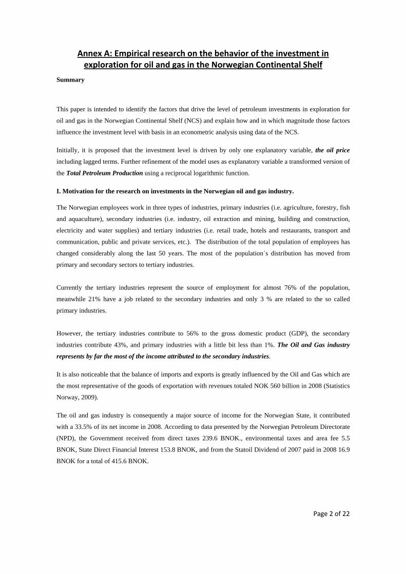
Annex A: Empirical research on the behavior of the investment in exploration for oil and gas in the Norwegian Continental Shelf
Page 2 of 22
Summary
This paper is intended to identify the factors that drive the level of petroleum investments in exploration for
oil and gas in the Norwegian Continental Shelf (NCS) and explain how and in which magnitude those factors
influence the investment level with basis in an econometric analysis using data of the NCS.
Initially, it is proposed that the investment level is driven by only one explanatory variable, the oil price
including lagged terms. Further refinement of the model uses as explanatory variable a transformed version of
the Total Petroleum Production using a reciprocal logarithmic function.
I. Motivation for the research on investments in the Norwegian oil and gas industry. The Norwegian employees work in three types of industries, primary industries (i.e. agriculture, forestry, fish
and aquaculture), secondary industries (i.e. industry, oil extraction and mining, building and construction,
electricity and water supplies) and tertiary industries (i.e. retail trade, hotels and restaurants, transport and
communication, public and private services, etc.). The distribution of the total population of employees has
changed considerably along the last 50 years. The most of the population´s distribution has moved from
primary and secondary sectors to tertiary industries.
Currently the tertiary industries represent the source of employment for almost 76% of the population,
meanwhile 21% have a job related to the secondary industries and only 3 % are related to the so called
primary industries.
However, the tertiary industries contribute to 56% to the gross domestic product (GDP), the secondary
industries contribute 43%, and primary industries with a little bit less than 1%. The Oil and Gas industry
represents by far the most of the income attributed to the secondary industries.
It is also noticeable that the balance of imports and exports is greatly influenced by the Oil and Gas which are
the most representative of the goods of exportation with revenues totaled NOK 560 billion in 2008 (Statistics
Norway, 2009).
The oil and gas industry is consequently a major source of income for the Norwegian State, it contributed
with a 33.5% of its net income in 2008. According to data presented by the Norwegian Petroleum Directorate
(NPD), the Government received from direct taxes 239.6 BNOK., environmental taxes and area fee 5.5
BNOK, State Direct Financial Interest 153.8 BNOK, and from the Statoil Dividend of 2007 paid in 2008 16.9
BNOK for a total of 415.6 BNOK.
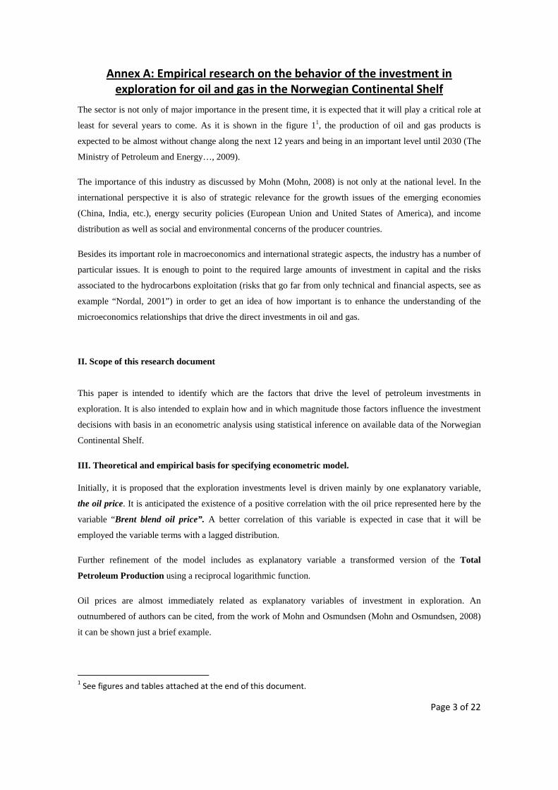
Annex A: Empirical research on the behavior of the investment in exploration for oil and gas in the Norwegian Continental Shelf
Page 3 of 22
The sector is not only of major importance in the present time, it is expected that it will play a critical role at
least for several years to come. As it is shown in the figure 11, the production of oil and gas products is
expected to be almost without change along the next 12 years and being in an important level until 2030 (The
Ministry of Petroleum and Energy…, 2009).
The importance of this industry as discussed by Mohn (Mohn, 2008) is not only at the national level. In the
international perspective it is also of strategic relevance for the growth issues of the emerging economies
(China, India, etc.), energy security policies (European Union and United States of America), and income
distribution as well as social and environmental concerns of the producer countries.
Besides its important role in macroeconomics and international strategic aspects, the industry has a number of
particular issues. It is enough to point to the required large amounts of investment in capital and the risks
associated to the hydrocarbons exploitation (risks that go far from only technical and financial aspects, see as
example “Nordal, 2001”) in order to get an idea of how important is to enhance the understanding of the
microeconomics relationships that drive the direct investments in oil and gas.
II. Scope of this research document
This paper is intended to identify which are the factors that drive the level of petroleum investments in
exploration. It is also intended to explain how and in which magnitude those factors influence the investment
decisions with basis in an econometric analysis using statistical inference on available data of the Norwegian
Continental Shelf.
III. Theoretical and empirical basis for specifying econometric model. Initially, it is proposed that the exploration investments level is driven mainly by one explanatory variable,
the oil price. It is anticipated the existence of a positive correlation with the oil price represented here by the
variable “Brent blend oil price”. A better correlation of this variable is expected in case that it will be
employed the variable terms with a lagged distribution.
Further refinement of the model includes as explanatory variable a transformed version of the Total
Petroleum Production using a reciprocal logarithmic function.
Oil prices are almost immediately related as explanatory variables of investment in exploration. An
outnumbered of authors can be cited, from the work of Mohn and Osmundsen (Mohn and Osmundsen, 2008)
it can be shown just a brief example.
1 See figures and tables attached at the end of this document.
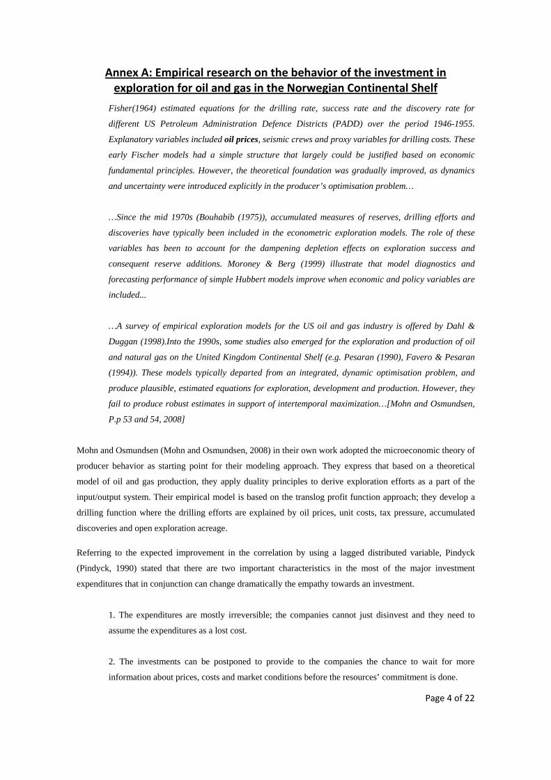
Annex A: Empirical research on the behavior of the investment in exploration for oil and gas in the Norwegian Continental Shelf
Page 4 of 22
Fisher(1964) estimated equations for the drilling rate, success rate and the discovery rate for
different US Petroleum Administration Defence Districts (PADD) over the period 1946-1955.
Explanatory variables included oil prices, seismic crews and proxy variables for drilling costs. These
early Fischer models had a simple structure that largely could be justified based on economic
fundamental principles. However, the theoretical foundation was gradually improved, as dynamics
and uncertainty were introduced explicitly in the producer’s optimisation problem…
…Since the mid 1970s (Bouhabib (1975)), accumulated measures of reserves, drilling efforts and
discoveries have typically been included in the econometric exploration models. The role of these
variables has been to account for the dampening depletion effects on exploration success and
consequent reserve additions. Moroney & Berg (1999) illustrate that model diagnostics and
forecasting performance of simple Hubbert models improve when economic and policy variables are
included...
…A survey of empirical exploration models for the US oil and gas industry is offered by Dahl &
Duggan (1998).Into the 1990s, some studies also emerged for the exploration and production of oil
and natural gas on the United Kingdom Continental Shelf (e.g. Pesaran (1990), Favero & Pesaran
(1994)). These models typically departed from an integrated, dynamic optimisation problem, and
produce plausible, estimated equations for exploration, development and production. However, they
fail to produce robust estimates in support of intertemporal maximization…[Mohn and Osmundsen,
P.p 53 and 54, 2008]
Mohn and Osmundsen (Mohn and Osmundsen, 2008) in their own work adopted the microeconomic theory of
producer behavior as starting point for their modeling approach. They express that based on a theoretical
model of oil and gas production, they apply duality principles to derive exploration efforts as a part of the
input/output system. Their empirical model is based on the translog profit function approach; they develop a
drilling function where the drilling efforts are explained by oil prices, unit costs, tax pressure, accumulated
discoveries and open exploration acreage.
Referring to the expected improvement in the correlation by using a lagged distributed variable, Pindyck
(Pindyck, 1990) stated that there are two important characteristics in the most of the major investment
expenditures that in conjunction can change dramatically the empathy towards an investment.
1. The expenditures are mostly irreversible; the companies cannot just disinvest and they need to
assume the expenditures as a lost cost.
2. The investments can be postponed to provide to the companies the chance to wait for more
information about prices, costs and market conditions before the resources’ commitment is done.
Annex A: Empirical research on the behavior of the investment in exploration for oil and gas in the Norwegian Continental Shelf
Page 5 of 22
Pindyck also explains in its model that the exploratory activity is the mean to accumulate or maintain a level
of reserves. He assumed that the exploratory activity expected outcome (the reserve additions discoveries”)
fall as cumulative discoveries increase. The level of the reserves chosen by the producers will depend on the
behavior of the production cost. If the production cost would be independent of the reserves the producers
would postpone much of their exploratory activity and maintain no reserves level.
Pindyck assumed that the production cost rise as the level of reserves decline, for the particular case of oil and
gas, he pointed out that at the level of individual reservoirs and fields, a lower amount of reserves means
higher extraction costs as the rate of physical output per unit of capital declines. He concludes that the
producers must determine an optimal reserve level- balancing revenues with exploration, production and
“user cost” of the depletion, (Pindyck, 1977).
IV. Presentation of the econometric model.
The data set used for this study is comprised of time series of the variables listed in table 1. The data set
shows the quarterly records from the first quarter of 1985 until the second quarter of 2008. It is assumed that
the 1000 SCM of natural gas = 1 SCM of NGL = 1 SCM condensate = 1 SCM oil = 1 ESCM Oil. Table 2
shows the original data set.
After a brief analysis of the data and the valuable literature listed in section III, it was considered that an
econometric model suitable to explain the level of investment in exploration could be a general distributed lag
model.
An unrestricted finite distributed lag model is specified as
y α ∑ β x ϵ ………………………………………………………………………(1)
Where bi is the multiplier of the effect of the variable xt-i. Consecuently yt would be explained by a finite
number of the variable x and the effect of its lagged values t-1 (Greene, 2003)
Remembering the proposed model explained in point No. 3, the exploration investments level is expected to
be driven by the existence of a positive correlation with the Oil price represented here by the variable “Brent
blend oil price”. A better correlation of this variable is expected in case is employed a lagged distribution of
the variable effects.
Hence, using the model of polynomial distributed lag in a particular form for this analysis the model would
be.
Annex A: Empirical research on the behavior of the investment in exploration for oil and gas in the Norwegian Continental Shelf
Page 6 of 22
∑ …..……………………………………………………..………..(2)
Where:
• IE = Investment in exploration, expressed in Millions of NOK, real value.
• BBOP = Brend blend oil price, expressed in USD per barrel, real value.
• =error.
In this case the number of lags for the explanatory variable BBOP was determined by comparing individually
the multiple coefficient of determination, R2, and adjusted R2, preferring the higher adjusted R2, that exists
between the variable IE and a generated model lag variable t-i, (k =1,2,3,4,5,6,7,8). 2
The creation of the lag data sets implied the loss of k observations in each set; consequently the missed data
was omitted in the calculation of the correlation between the variables. Table 3 shows the results of the
multiple regression models for investments in exploration explained by the Brent blend oil Price and its
lagged values until 8 quarterly lags.
As shown in table 3, the peak of correlation Adjusted R2, and one of the minimum standard error of the
estimate is found in the model with lag 4. Consequently it was chosen that the most appropriate number of
lagged terms to be considered was 4.
If we assume that the model satisfies the normal properties of the regression by least squares estimators.
• Linearity of the relationship between dependent and independent variables.
• Independence of the errors (there are no serial correlations).
• Homoscedasticity or constant variance of the errors.
o 3.1) versus time.
o 3.2) versus the predictions (or versus any independent variable).
o 3.3) normality of the error distribution.
And that the lag length p is known, the model can be solved as a classical regression model.
This model; however have many weaknesses as it will be discussed in the next section when the results are
shown, just to mention the most important is that is expected to be serially correlated and the multi-
2 To do the calculations and the figures shown in this document it was used the Microsoft Excel Software (2007) and the StatTools Add‐in for Microsoft Excel by Palisade Corporation (2010).
Annex A: Empirical research on the behavior of the investment in exploration for oil and gas in the Norwegian Continental Shelf
Page 7 of 22
collinearity of the model is expected to be severe. To solve this problem it is suggested to employ a more
refined way to calculate the weight bi (the multiplier of the effect of the variable xt-i), the polynomial lag
model.
The invention of this model is attributed to Almon (Almon, 1965).
The polynomial model assumes that the true distribution of lag coefficients can be well approximate
by a low-order polynomial.
2) , 0,1… ,
Substituting 2 in 1 an collecting terms it is obtained
∑ ∑ ∑ ……………….……….(3)
………………………………………………………………..…(4)
Each zjt ia a linear combination of the current and the p lagged values of xt . With the
assumption of strict exogenety of xt, γ and (a0,a1,…,aq) can be estimated by ordinary or generalized
least squares…
(Greene, P.p. 565-566, 2003)
The difficulties of using Almon's technique in the estimation of distributed lags have been extensively
investigated. Thomas made a discussion of the Almon’s model resulting in a critical analysis of the
“conventional criteria for choosing the “best” model (such as goodness of fit, the statistical significance of
the individual parameter estimate or their sums, and an analysis of autocorrelation) demonstrates the
problems of choosing the appropriate combination of lag length and degree of polynomial” [Thomas, P.P.
175, 1977].
V. Presentation of econometric results for the original model.
Table 4 shows the estimated parameters of the model. Figure 2 shows a plot comparison between the actual
records of investment level and the model results. It is inferred that the investment in exploration is positively
affected by the increase of the price of oil, being more noticeable between the second and fourth month of the
increase in the oil price.
Annex A: Empirical research on the behavior of the investment in exploration for oil and gas in the Norwegian Continental Shelf
Page 8 of 22
V.1 Commentaries on the reliability of the model. As commented before, when it is used the econometric
modeling of time series by distributed lag models is common to have violations of independence between the
variables. This fact is evidenced by serial correlation between the residuals; a typical tool to detect these
phenomena is by the calculation of the autocorrelation or trough a Durbin Watson test.
In this case it is shown the correlation coefficients for the residuals (table 4), and the autocorrelation plot of
the residuals (figure 3), it is evident that exists an autocorrelation in the residuals. This enounced observation
open an ample space to search for a model correction, either by consider transformations, the application of
techniques like Almon’s, identification and correction for seasonality’s or the search for additional
explanatory variables, just to mention some.
VI. Model Correction
To correct the model is proposed the use of an additional explanatory variable based in the theory of Pindyck
(Pindyck, 1997) previously referred at the end of section III. It will be transformed the variable Total
Petroleum Production using a reciprocal logarithmic function for its cumulative value to be related linearly
to the corrected model.
It means:
NEV = New Explanatory variable
NEVt = 1/log (∑
Where:
TPPt = Total Petroleum production in time t.
Q = Consecutive posterior quarter with “1985Q1” as Q=1, !985Q2 as Q=2…
The transformed values of the NEV are shown in table 6.
Then the corrected model is formulated as following:
∑ ……………………………………………………………….(5)
Where:
Annex A: Empirical research on the behavior of the investment in exploration for oil and gas in the Norwegian Continental Shelf
Page 9 of 22
• IE = Investment in exploration, expressed in Millions of NOK, real value.
• BBOP = Brend blend oil price, expressed in USD per barrel, real value.
• NEV = New Explanatory variable, as defined above.
• =error.
VII. Presentation of the econometric results and conclusions using the corrected model.
Table 7 shows the estimated parameters of the corrected model. Figure 4 shows a plot comparison between
the actual records of investment level and the results of the corrected model.
There is a noticeable improvement in the coefficients of correlation multiple, R2, and adjusted R2 with
perceptible changes in the coefficients. It is then inferred that the change in price of oil is positively correlated
to the increase of investment in the same period. However there is also an adjustment mechanism to moderate
the reaction toward the oil and gas commodities markets.
In that way it seems that the investments have a positive correlation in the same quarter against the change in
the oil price, a negative correlation adjust in the first quarter after the level of investment, positive correlation
affects the investment in the second quarter, negative correlation is perceptible again in the third quarter and a
positive correlation also is noticeable in the fourth quarter after a change in the oil and gas prices.
Despite the adjustment mechanisms the oil price has a positive correlation with the level of investment
increasing or decreasing approximately 16 millions of NOK four quarters after the price is adjusted in 1 USD.
The new explanatory variable also suggests that the depletion of the reservoirs is an element that the oil
companies consider as a long term trend. As the amount of oil and gas produced is increased there is an
inclination to diminish the level of investment in exploration, presumably since it is considered that the
probability of commercial success become smaller.
VII.1 Commentaries on the reliability of the model. Correlation coefficients for the residuals (table 8), and
the autocorrelation plot of the residuals (figure 5), Show a considerable improvement regarding the presence
of evidence of autocorrelation in the residuals. Although it may be judged still to be too high, the relatively
small error in the model make to think that is a reliable to predict the behavior of investment levels in
exploration in the Norwegian Continental Shelf.
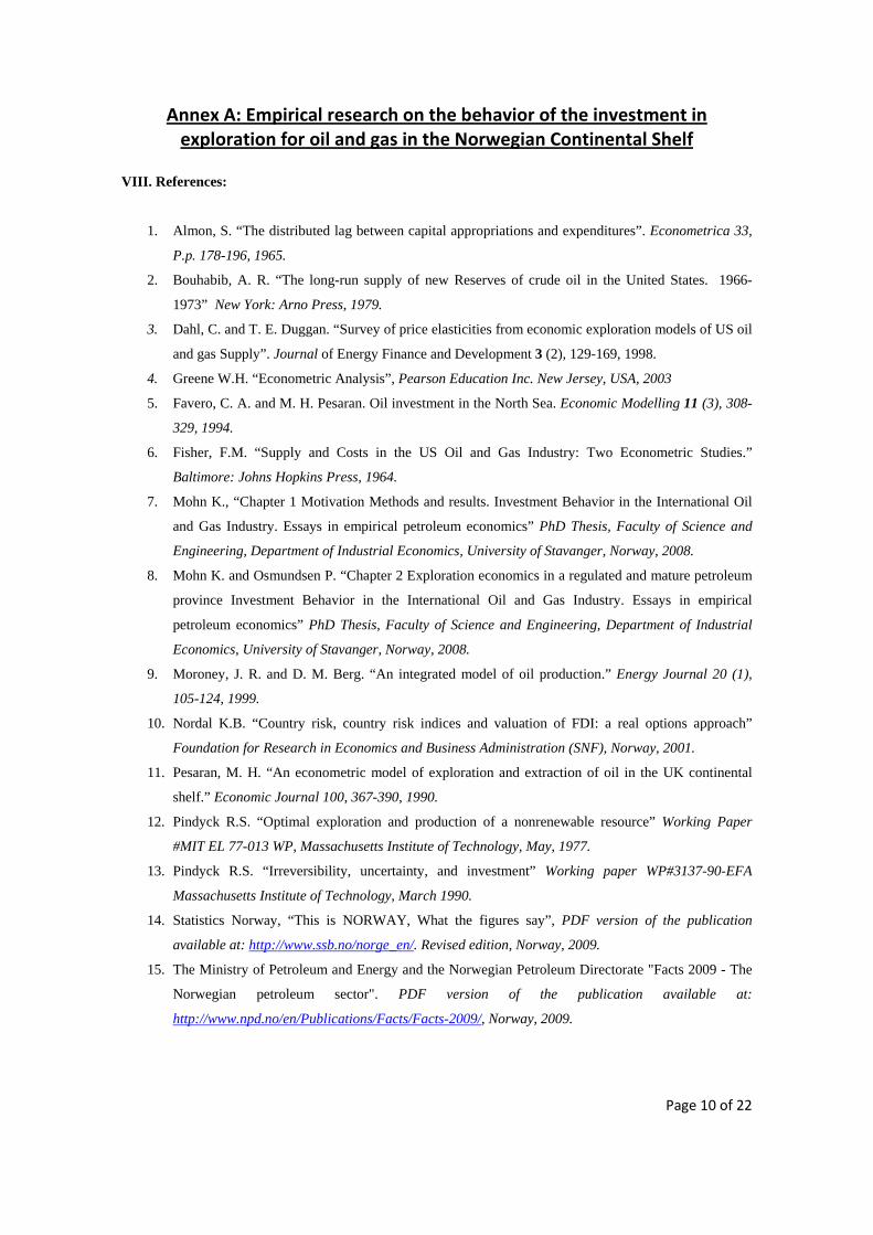
Annex A: Empirical research on the behavior of the investment in exploration for oil and gas in the Norwegian Continental Shelf
Page 10 of 22
VIII. References:
1. Almon, S. “The distributed lag between capital appropriations and expenditures”. Econometrica 33,
P.p. 178-196, 1965.
2. Bouhabib, A. R. “The long-run supply of new Reserves of crude oil in the United States. 1966-
1973” New York: Arno Press, 1979.
3. Dahl, C. and T. E. Duggan. “Survey of price elasticities from economic exploration models of US oil
and gas Supply”. Journal of Energy Finance and Development 3 (2), 129-169, 1998.
4. Greene W.H. “Econometric Analysis”, Pearson Education Inc. New Jersey, USA, 2003
5. Favero, C. A. and M. H. Pesaran. Oil investment in the North Sea. Economic Modelling 11 (3), 308-
329, 1994.
6. Fisher, F.M. “Supply and Costs in the US Oil and Gas Industry: Two Econometric Studies.”
Baltimore: Johns Hopkins Press, 1964.
7. Mohn K., “Chapter 1 Motivation Methods and results. Investment Behavior in the International Oil
and Gas Industry. Essays in empirical petroleum economics” PhD Thesis, Faculty of Science and
Engineering, Department of Industrial Economics, University of Stavanger, Norway, 2008.
8. Mohn K. and Osmundsen P. “Chapter 2 Exploration economics in a regulated and mature petroleum
province Investment Behavior in the International Oil and Gas Industry. Essays in empirical
petroleum economics” PhD Thesis, Faculty of Science and Engineering, Department of Industrial
Economics, University of Stavanger, Norway, 2008.
9. Moroney, J. R. and D. M. Berg. “An integrated model of oil production.” Energy Journal 20 (1),
105-124, 1999.
10. Nordal K.B. “Country risk, country risk indices and valuation of FDI: a real options approach”
Foundation for Research in Economics and Business Administration (SNF), Norway, 2001.
11. Pesaran, M. H. “An econometric model of exploration and extraction of oil in the UK continental
shelf.” Economic Journal 100, 367-390, 1990.
12. Pindyck R.S. “Optimal exploration and production of a nonrenewable resource” Working Paper
#MIT EL 77-013 WP, Massachusetts Institute of Technology, May, 1977.
13. Pindyck R.S. “Irreversibility, uncertainty, and investment” Working paper WP#3137-90-EFA
Massachusetts Institute of Technology, March 1990.
14. Statistics Norway, “This is NORWAY, What the figures say”, PDF version of the publication
available at: http://www.ssb.no/norge_en/. Revised edition, Norway, 2009.
15. The Ministry of Petroleum and Energy and the Norwegian Petroleum Directorate "Facts 2009 - The
Norwegian petroleum sector". PDF version of the publication available at:
http://www.npd.no/en/Publications/Facts/Facts-2009/, Norway, 2009.

Annex A: Empirical research on the behavior of the investment in exploration for oil and gas in the Norwegian Continental Shelf
Page 11 of 22
16. Thomas J.J. “Some problems in the use of Almon's technique in the estimation of distributed lags”,
The London School of Economics and Political Science, Houghton Street, WC2A 2 AE London,
Published in Empirical Economics Volume 2, Number 3, September 1977.
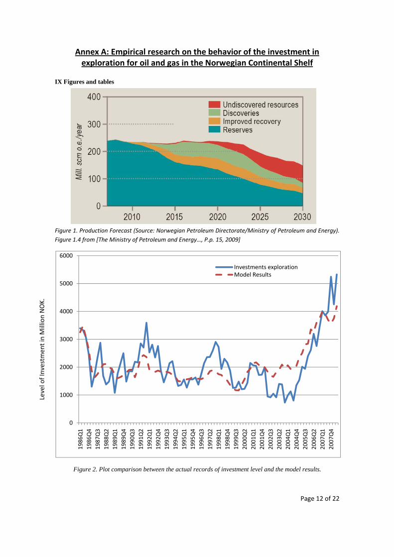
Annex A: Empirical research on the behavior of the investment in exploration for oil and gas in the Norwegian Continental Shelf
Page 12 of 22
IX Figures and tables
Figure 1. Production Forecast (Source: Norwegian Petroleum Directorate/Ministry of Petroleum and Energy). Figure 1.4 from [The Ministry of Petroleum and Energy…, P.p. 15, 2009]
Figure 2. Plot comparison between the actual records of investment level and the model results.
0
1000
2000
3000
4000
5000
6000
1986
Q1
1986
Q4
1987
Q3
1988
Q2
1989
Q1
1989
Q4
1990
Q3
1991
Q2
1992
Q1
1992
Q4
1993
Q3
1994
Q2
1995
Q1
1995
Q4
1996
Q3
1997
Q2
1998
Q1
1998
Q4
1999
Q3
2000
Q2
2001
Q1
2001
Q4
2002
Q3
2003
Q2
2004
Q1
2004
Q4
2005
Q3
2006
Q2
2007
Q1
2007
Q4
Investments explorationModel Results
Level of Investm
ent in Million NOK.
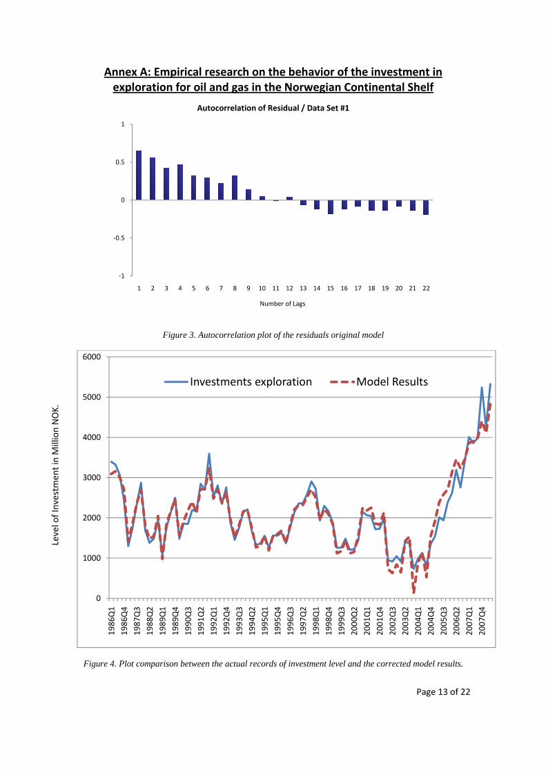
Annex A: Empirical research on the behavior of the investment in exploration for oil and gas in the Norwegian Continental Shelf
Page 13 of 22
Figure 3. Autocorrelation plot of the residuals original model
Figure 4. Plot comparison between the actual records of investment level and the corrected model results.
‐1
‐0.5
0
0.5
1
1 2 3 4 5 6 7 8 9 10 11 12 13 14 15 16 17 18 19 20 21 22
Number of Lags
Autocorrelation of Residual / Data Set #1
0
1000
2000
3000
4000
5000
6000
1986
Q1
1986
Q4
1987
Q3
1988
Q2
1989
Q1
1989
Q4
1990
Q3
1991
Q2
1992
Q1
1992
Q4
1993
Q3
1994
Q2
1995
Q1
1995
Q4
1996
Q3
1997
Q2
1998
Q1
1998
Q4
1999
Q3
2000
Q2
2001
Q1
2001
Q4
2002
Q3
2003
Q2
2004
Q1
2004
Q4
2005
Q3
2006
Q2
2007
Q1
2007
Q4
Investments exploration Model Results
Level of Investm
ent in Million NOK.
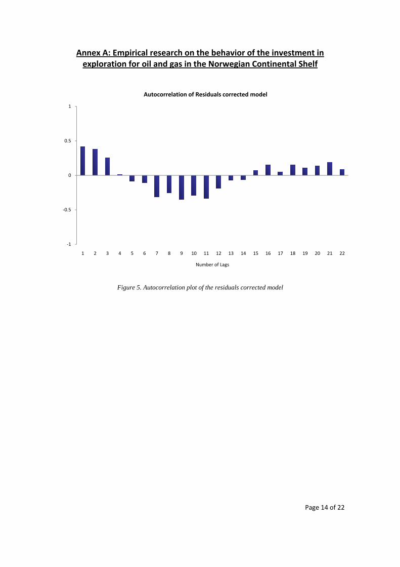
Annex A: Empirical research on the behavior of the investment in exploration for oil and gas in the Norwegian Continental Shelf
Page 14 of 22
Figure 5. Autocorrelation plot of the residuals corrected model
‐1
‐0.5
0
0.5
1
1 2 3 4 5 6 7 8 9 10 11 12 13 14 15 16 17 18 19 20 21 22
Number of Lags
Autocorrelation of Residuals corrected model
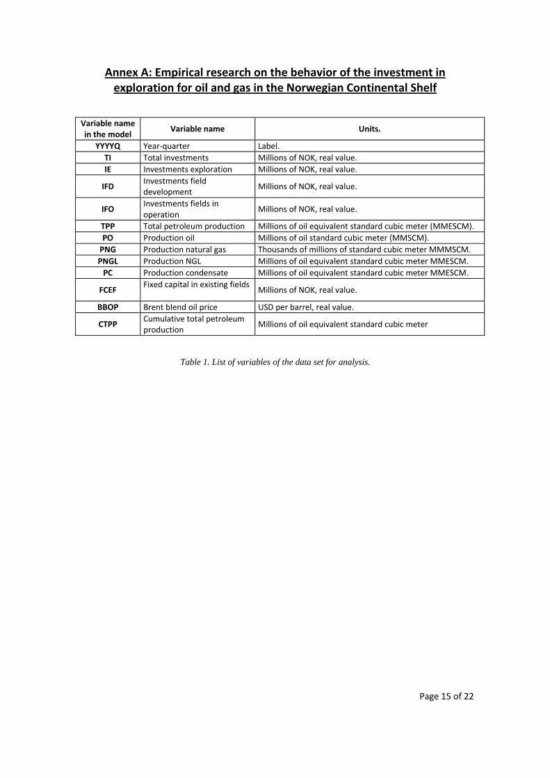
Annex A: Empirical research on the behavior of the investment in exploration for oil and gas in the Norwegian Continental Shelf
Page 15 of 22
Variable name in the model
Variable name Units.
YYYYQ Year‐quarter Label.TI Total investments Millions of NOK, real value.IE Investments exploration Millions of NOK, real value.
IFD Investments field development
Millions of NOK, real value.
IFO Investments fields in operation
Millions of NOK, real value.
TPP Total petroleum production Millions of oil equivalent standard cubic meter (MMESCM).PO Production oil Millions of oil standard cubic meter (MMSCM). PNG Production natural gas Thousands of millions of standard cubic meter MMMSCM.PNGL Production NGL Millions of oil equivalent standard cubic meter MMESCM.PC Production condensate Millions of oil equivalent standard cubic meter MMESCM.
FCEF Fixed capital in existing fields
Millions of NOK, real value.
BBOP Brent blend oil price USD per barrel, real value.
CTPP Cumulative total petroleum production
Millions of oil equivalent standard cubic meter
Table 1. List of variables of the data set for analysis.
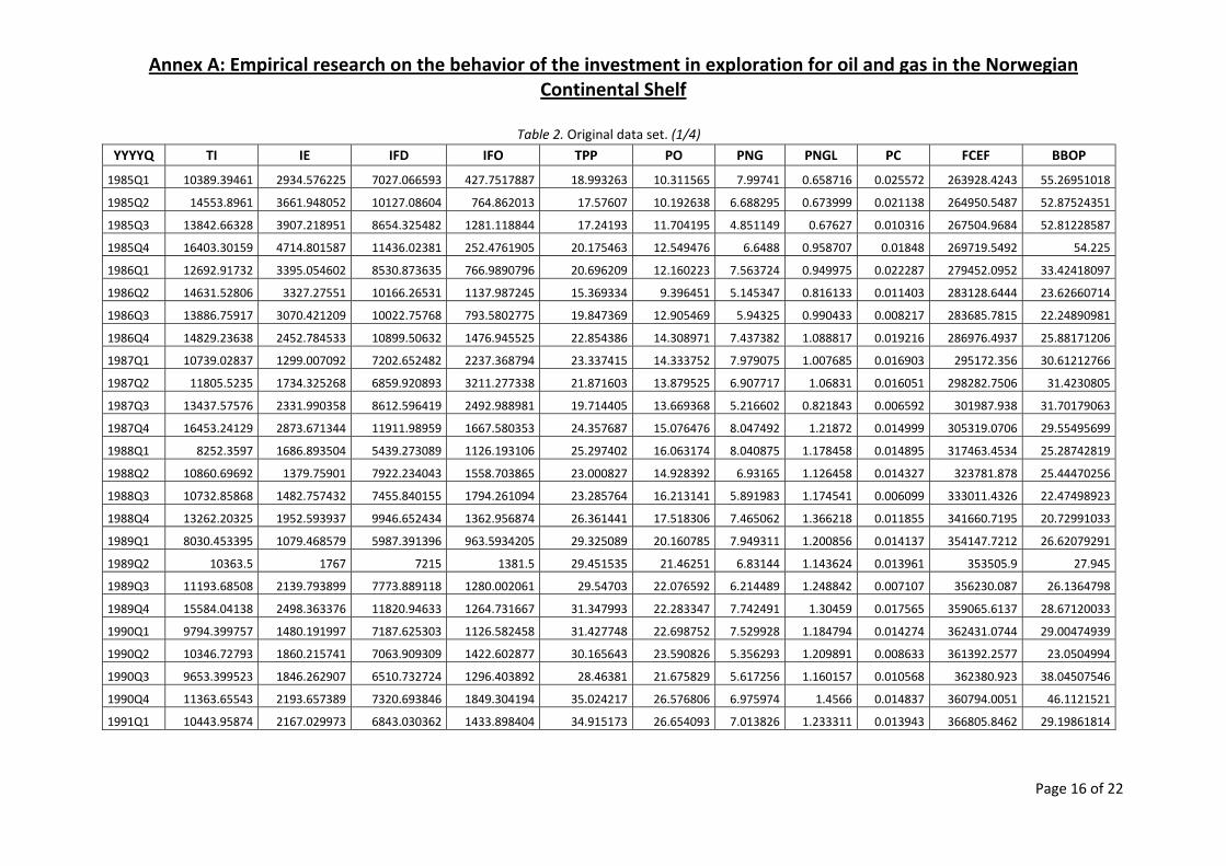
Annex A: Empirical research on the behavior of the investment in exploration for oil and gas in the Norwegian Continental Shelf
Page 16 of 22
Table 2. Original data set. (1/4)
YYYYQ TI IE IFD IFO TPP PO PNG PNGL PC FCEF BBOP
1985Q1 10389.39461 2934.576225 7027.066593 427.7517887 18.993263 10.311565 7.99741 0.658716 0.025572 263928.4243 55.26951018
1985Q2 14553.8961 3661.948052 10127.08604 764.862013 17.57607 10.192638 6.688295 0.673999 0.021138 264950.5487 52.87524351
1985Q3 13842.66328 3907.218951 8654.325482 1281.118844 17.24193 11.704195 4.851149 0.67627 0.010316 267504.9684 52.81228587
1985Q4 16403.30159 4714.801587 11436.02381 252.4761905 20.175463 12.549476 6.6488 0.958707 0.01848 269719.5492 54.225
1986Q1 12692.91732 3395.054602 8530.873635 766.9890796 20.696209 12.160223 7.563724 0.949975 0.022287 279452.0952 33.42418097
1986Q2 14631.52806 3327.27551 10166.26531 1137.987245 15.369334 9.396451 5.145347 0.816133 0.011403 283128.6444 23.62660714
1986Q3 13886.75917 3070.421209 10022.75768 793.5802775 19.847369 12.905469 5.94325 0.990433 0.008217 283685.7815 22.24890981
1986Q4 14829.23638 2452.784533 10899.50632 1476.945525 22.854386 14.308971 7.437382 1.088817 0.019216 286976.4937 25.88171206
1987Q1 10739.02837 1299.007092 7202.652482 2237.368794 23.337415 14.333752 7.979075 1.007685 0.016903 295172.356 30.61212766
1987Q2 11805.5235 1734.325268 6859.920893 3211.277338 21.871603 13.879525 6.907717 1.06831 0.016051 298282.7506 31.4230805
1987Q3 13437.57576 2331.990358 8612.596419 2492.988981 19.714405 13.669368 5.216602 0.821843 0.006592 301987.938 31.70179063
1987Q4 16453.24129 2873.671344 11911.98959 1667.580353 24.357687 15.076476 8.047492 1.21872 0.014999 305319.0706 29.55495699
1988Q1 8252.3597 1686.893504 5439.273089 1126.193106 25.297402 16.063174 8.040875 1.178458 0.014895 317463.4534 25.28742819
1988Q2 10860.69692 1379.75901 7922.234043 1558.703865 23.000827 14.928392 6.93165 1.126458 0.014327 323781.878 25.44470256
1988Q3 10732.85868 1482.757432 7455.840155 1794.261094 23.285764 16.213141 5.891983 1.174541 0.006099 333011.4326 22.47498923
1988Q4 13262.20325 1952.593937 9946.652434 1362.956874 26.361441 17.518306 7.465062 1.366218 0.011855 341660.7195 20.72991033
1989Q1 8030.453395 1079.468579 5987.391396 963.5934205 29.325089 20.160785 7.949311 1.200856 0.014137 354147.7212 26.62079291
1989Q2 10363.5 1767 7215 1381.5 29.451535 21.46251 6.83144 1.143624 0.013961 353505.9 27.945
1989Q3 11193.68508 2139.793899 7773.889118 1280.002061 29.54703 22.076592 6.214489 1.248842 0.007107 356230.087 26.1364798
1989Q4 15584.04138 2498.363376 11820.94633 1264.731667 31.347993 22.283347 7.742491 1.30459 0.017565 359065.6137 28.67120033
1990Q1 9794.399757 1480.191997 7187.625303 1126.582458 31.427748 22.698752 7.529928 1.184794 0.014274 362431.0744 29.00474939
1990Q2 10346.72793 1860.215741 7063.909309 1422.602877 30.165643 23.590826 5.356293 1.209891 0.008633 361392.2577 23.0504994
1990Q3 9653.399523 1846.262907 6510.732724 1296.403892 28.46381 21.675829 5.617256 1.160157 0.010568 362380.923 38.04507546
1990Q4 11363.65543 2193.657389 7320.693846 1849.304194 35.024217 26.576806 6.975974 1.4566 0.014837 360794.0051 46.1121521
1991Q1 10443.95874 2167.029973 6843.030362 1433.898404 34.915173 26.654093 7.013826 1.233311 0.013943 366805.8462 29.19861814
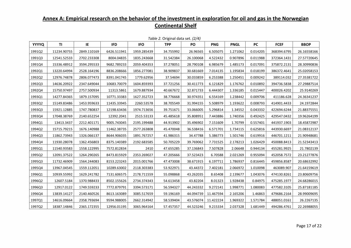
Annex A: Empirical research on the behavior of the investment in exploration for oil and gas in the Norwegian Continental Shelf
Page 17 of 22
Table 2. Original data set. (2/4)
YYYYQ TI IE IFD IFO TPP PO PNG PNGL PC FCEF BBOP
1991Q2 11234.90755 2849.110169 6426.511941 1959.285439 34.755992 26.96565 6.505075 1.271062 0.014205 368394.6795 26.16558166
1991Q3 12541.52533 2702.233308 8004.04835 1835.243668 31.542384 26.100068 4.522432 0.907896 0.011988 372364.1431 27.57720645
1991Q4 15336.48912 3594.295533 9682.789233 2059.404353 37.278051 28.790108 6.985679 1.485173 0.017091 375872.2131 28.30990836
1992Q1 13220.64994 2528.164196 8836.208666 1856.277081 38.909837 30.681669 7.014135 1.195834 0.018199 386372.4641 25.02058153
1992Q2 12976.74878 2806.077473 8391.041745 1779.62956 37.54694 30.033859 6.253388 1.250451 0.009242 389114.032 27.35381722
1992Q3 14636.20922 2347.649044 10683.70079 1604.859393 37.721256 30.411773 6.121829 1.176762 0.010892 394736.5838 27.29887514
1992Q4 15750.97497 2757.500934 11313.5861 1679.887934 40.667672 32.871733 6.444307 1.336185 0.015447 400026.4202 25.9140269
1993Q1 14277.84365 1879.157095 10771.33383 1627.352723 38.776668 30.974351 6.554169 1.238442 0.009706 411186.628 24.36341237
1993Q2 15149.83486 1453.959633 11435.33945 2260.53578 38.705549 31.994155 5.508979 1.193622 0.008793 414901.4433 24.1972844
1993Q3 15921.12885 1747.780837 12198.63436 1974.713656 39.751671 33.066005 5.296814 1.34552 0.043332 422694.6244 21.88375551
1993Q4 17048.38769 2140.652254 12392.2041 2515.53133 45.485618 35.808951 7.443886 1.740356 0.492425 429547.0432 19.96264199
1994Q1 13413.3437 2212.401171 9005.743045 2195.199488 44.913902 35.496902 7.151609 1.70799 0.557401 441937.1903 18.45872987
1994Q2 15715.79215 1676.140988 11462.38735 2577.263808 45.470048 36.538416 6.571701 1.734115 0.625816 443930.6697 21.08312137
1994Q3 11862.73943 1326.066137 8644.906035 1891.767257 41.986315 34.47788 5.386773 1.501746 0.619916 446701.1211 21.90948681
1994Q4 11930.28078 1362.456803 8375.140389 2192.683585 50.705229 39.769062 7.731525 2.178213 1.026429 450088.8413 21.52343413
1995Q1 11540.93583 1558.122995 7572.812834 2410 47.655285 37.136843 7.507828 2.06648 0.944134 455281.9925 21.7802139
1995Q2 12091.37522 1264.290265 8473.815929 2353.269027 47.205666 37.523423 6.70588 2.021269 0.955094 452058.7572 23.21277876
1995Q3 11732.46909 1564.244083 8153.223243 2015.001766 47.473008 38.671915 6.197711 1.786937 0.816445 459856.8587 20.68632992
1995Q4 13967.04545 1559.112051 10289.63002 2118.303383 53.922971 43.44372 7.402181 2.066972 1.010098 463089.907 21.64159619
1996Q1 10939.55992 1629.241782 7131.606575 2178.711559 55.098868 43.262035 8.65408 2.139677 1.043076 474130.8261 23.80609756
1996Q2 12607.5184 1370.988433 8502.155626 2734.374343 54.613458 43.82204 8.01323 1.928438 0.84975 475285.1977 24.68286015
1996Q3 12917.0122 1749.559233 7772.879791 3394.573171 56.594327 44.243332 9.272141 1.998771 1.080083 477582.3105 25.87181185
1996Q4 13839.14127 2140.460526 8613.163089 3085.517659 59.196169 44.094739 11.467594 2.165206 1.46863 479686.2164 28.99009695
1997Q1 14616.09664 2358.793694 9594.988005 2662.314942 58.539404 43.576074 11.422224 1.969322 1.571784 488051.0161 26.2267135
1997Q2 18387.14846 2365.172355 12956.01195 3065.964164 57.457357 44.523246 9.215334 2.037328 1.681449 494286.4761 22.26988055
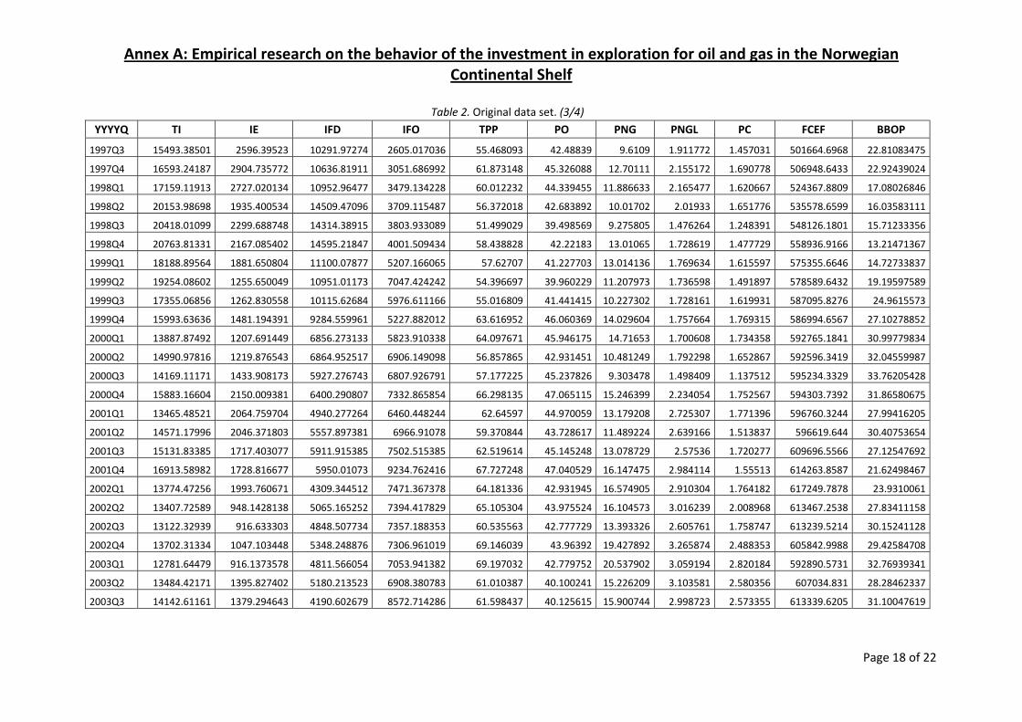
Annex A: Empirical research on the behavior of the investment in exploration for oil and gas in the Norwegian Continental Shelf
Page 18 of 22
Table 2. Original data set. (3/4)
YYYYQ TI IE IFD IFO TPP PO PNG PNGL PC FCEF BBOP
1997Q3 15493.38501 2596.39523 10291.97274 2605.017036 55.468093 42.48839 9.6109 1.911772 1.457031 501664.6968 22.81083475
1997Q4 16593.24187 2904.735772 10636.81911 3051.686992 61.873148 45.326088 12.70111 2.155172 1.690778 506948.6433 22.92439024
1998Q1 17159.11913 2727.020134 10952.96477 3479.134228 60.012232 44.339455 11.886633 2.165477 1.620667 524367.8809 17.08026846
1998Q2 20153.98698 1935.400534 14509.47096 3709.115487 56.372018 42.683892 10.01702 2.01933 1.651776 535578.6599 16.03583111
1998Q3 20418.01099 2299.688748 14314.38915 3803.933089 51.499029 39.498569 9.275805 1.476264 1.248391 548126.1801 15.71233356
1998Q4 20763.81331 2167.085402 14595.21847 4001.509434 58.438828 42.22183 13.01065 1.728619 1.477729 558936.9166 13.21471367
1999Q1 18188.89564 1881.650804 11100.07877 5207.166065 57.62707 41.227703 13.014136 1.769634 1.615597 575355.6646 14.72733837
1999Q2 19254.08602 1255.650049 10951.01173 7047.424242 54.396697 39.960229 11.207973 1.736598 1.491897 578589.6432 19.19597589
1999Q3 17355.06856 1262.830558 10115.62684 5976.611166 55.016809 41.441415 10.227302 1.728161 1.619931 587095.8276 24.9615573
1999Q4 15993.63636 1481.194391 9284.559961 5227.882012 63.616952 46.060369 14.029604 1.757664 1.769315 586994.6567 27.10278852
2000Q1 13887.87492 1207.691449 6856.273133 5823.910338 64.097671 45.946175 14.71653 1.700608 1.734358 592765.1841 30.99779834
2000Q2 14990.97816 1219.876543 6864.952517 6906.149098 56.857865 42.931451 10.481249 1.792298 1.652867 592596.3419 32.04559987
2000Q3 14169.11171 1433.908173 5927.276743 6807.926791 57.177225 45.237826 9.303478 1.498409 1.137512 595234.3329 33.76205428
2000Q4 15883.16604 2150.009381 6400.290807 7332.865854 66.298135 47.065115 15.246399 2.234054 1.752567 594303.7392 31.86580675
2001Q1 13465.48521 2064.759704 4940.277264 6460.448244 62.64597 44.970059 13.179208 2.725307 1.771396 596760.3244 27.99416205
2001Q2 14571.17996 2046.371803 5557.897381 6966.91078 59.370844 43.728617 11.489224 2.639166 1.513837 596619.644 30.40753654
2001Q3 15131.83385 1717.403077 5911.915385 7502.515385 62.519614 45.145248 13.078729 2.57536 1.720277 609696.5566 27.12547692
2001Q4 16913.58982 1728.816677 5950.01073 9234.762416 67.727248 47.040529 16.147475 2.984114 1.55513 614263.8587 21.62498467
2002Q1 13774.47256 1993.760671 4309.344512 7471.367378 64.181336 42.931945 16.574905 2.910304 1.764182 617249.7878 23.9310061
2002Q2 13407.72589 948.1428138 5065.165252 7394.417829 65.105304 43.975524 16.104573 3.016239 2.008968 613467.2538 27.83411158
2002Q3 13122.32939 916.633303 4848.507734 7357.188353 60.535563 42.777729 13.393326 2.605761 1.758747 613239.5214 30.15241128
2002Q4 13702.31334 1047.103448 5348.248876 7306.961019 69.146039 43.96392 19.427892 3.265874 2.488353 605842.9988 29.42584708
2003Q1 12781.64479 916.1373578 4811.566054 7053.941382 69.197032 42.779752 20.537902 3.059194 2.820184 592890.5731 32.76939341
2003Q2 13484.42171 1395.827402 5180.213523 6908.380783 61.010387 40.100241 15.226209 3.103581 2.580356 607034.831 28.28462337
2003Q3 14142.61161 1379.294643 4190.602679 8572.714286 61.598437 40.125615 15.900744 2.998723 2.573355 613339.6205 31.10047619
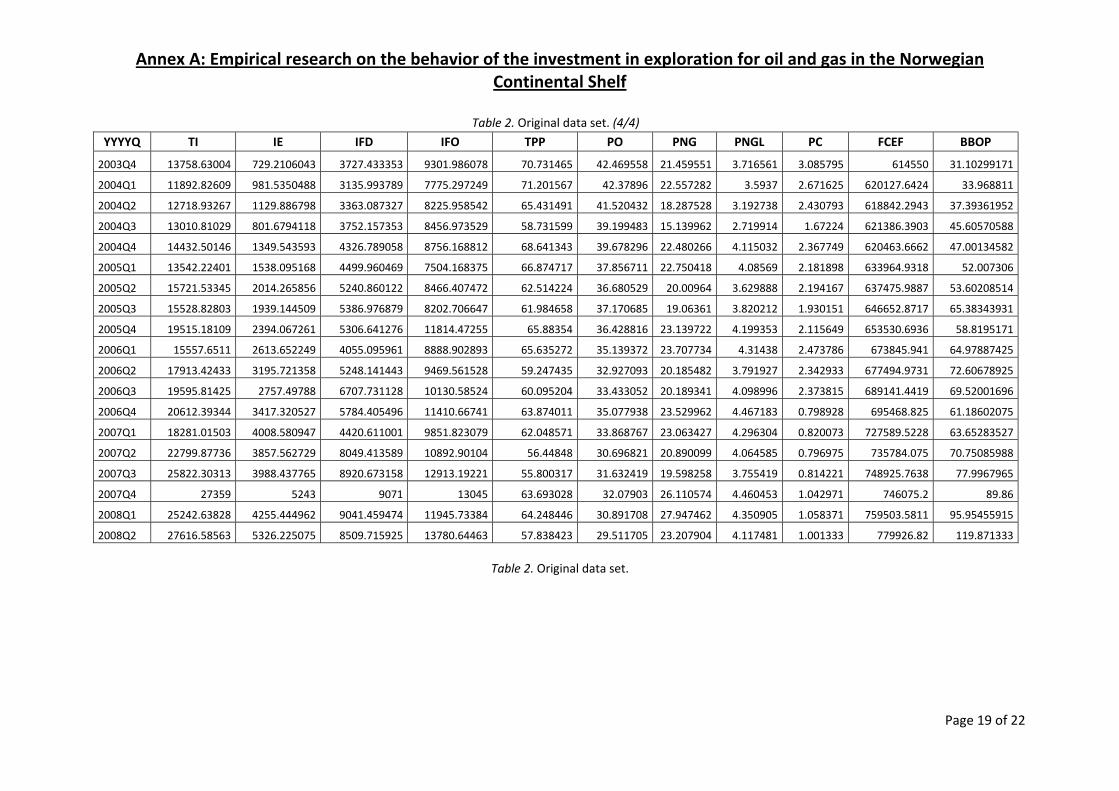
Annex A: Empirical research on the behavior of the investment in exploration for oil and gas in the Norwegian Continental Shelf
Page 19 of 22
Table 2. Original data set. (4/4)
YYYYQ TI IE IFD IFO TPP PO PNG PNGL PC FCEF BBOP
2003Q4 13758.63004 729.2106043 3727.433353 9301.986078 70.731465 42.469558 21.459551 3.716561 3.085795 614550 31.10299171
2004Q1 11892.82609 981.5350488 3135.993789 7775.297249 71.201567 42.37896 22.557282 3.5937 2.671625 620127.6424 33.968811
2004Q2 12718.93267 1129.886798 3363.087327 8225.958542 65.431491 41.520432 18.287528 3.192738 2.430793 618842.2943 37.39361952
2004Q3 13010.81029 801.6794118 3752.157353 8456.973529 58.731599 39.199483 15.139962 2.719914 1.67224 621386.3903 45.60570588
2004Q4 14432.50146 1349.543593 4326.789058 8756.168812 68.641343 39.678296 22.480266 4.115032 2.367749 620463.6662 47.00134582
2005Q1 13542.22401 1538.095168 4499.960469 7504.168375 66.874717 37.856711 22.750418 4.08569 2.181898 633964.9318 52.007306
2005Q2 15721.53345 2014.265856 5240.860122 8466.407472 62.514224 36.680529 20.00964 3.629888 2.194167 637475.9887 53.60208514
2005Q3 15528.82803 1939.144509 5386.976879 8202.706647 61.984658 37.170685 19.06361 3.820212 1.930151 646652.8717 65.38343931
2005Q4 19515.18109 2394.067261 5306.641276 11814.47255 65.88354 36.428816 23.139722 4.199353 2.115649 653530.6936 58.8195171
2006Q1 15557.6511 2613.652249 4055.095961 8888.902893 65.635272 35.139372 23.707734 4.31438 2.473786 673845.941 64.97887425
2006Q2 17913.42433 3195.721358 5248.141443 9469.561528 59.247435 32.927093 20.185482 3.791927 2.342933 677494.9731 72.60678925
2006Q3 19595.81425 2757.49788 6707.731128 10130.58524 60.095204 33.433052 20.189341 4.098996 2.373815 689141.4419 69.52001696
2006Q4 20612.39344 3417.320527 5784.405496 11410.66741 63.874011 35.077938 23.529962 4.467183 0.798928 695468.825 61.18602075
2007Q1 18281.01503 4008.580947 4420.611001 9851.823079 62.048571 33.868767 23.063427 4.296304 0.820073 727589.5228 63.65283527
2007Q2 22799.87736 3857.562729 8049.413589 10892.90104 56.44848 30.696821 20.890099 4.064585 0.796975 735784.075 70.75085988
2007Q3 25822.30313 3988.437765 8920.673158 12913.19221 55.800317 31.632419 19.598258 3.755419 0.814221 748925.7638 77.9967965
2007Q4 27359 5243 9071 13045 63.693028 32.07903 26.110574 4.460453 1.042971 746075.2 89.86
2008Q1 25242.63828 4255.444962 9041.459474 11945.73384 64.248446 30.891708 27.947462 4.350905 1.058371 759503.5811 95.95455915
2008Q2 27616.58563 5326.225075 8509.715925 13780.64463 57.838423 29.511705 23.207904 4.117481 1.001333 779926.82 119.871333
Table 2. Original data set.
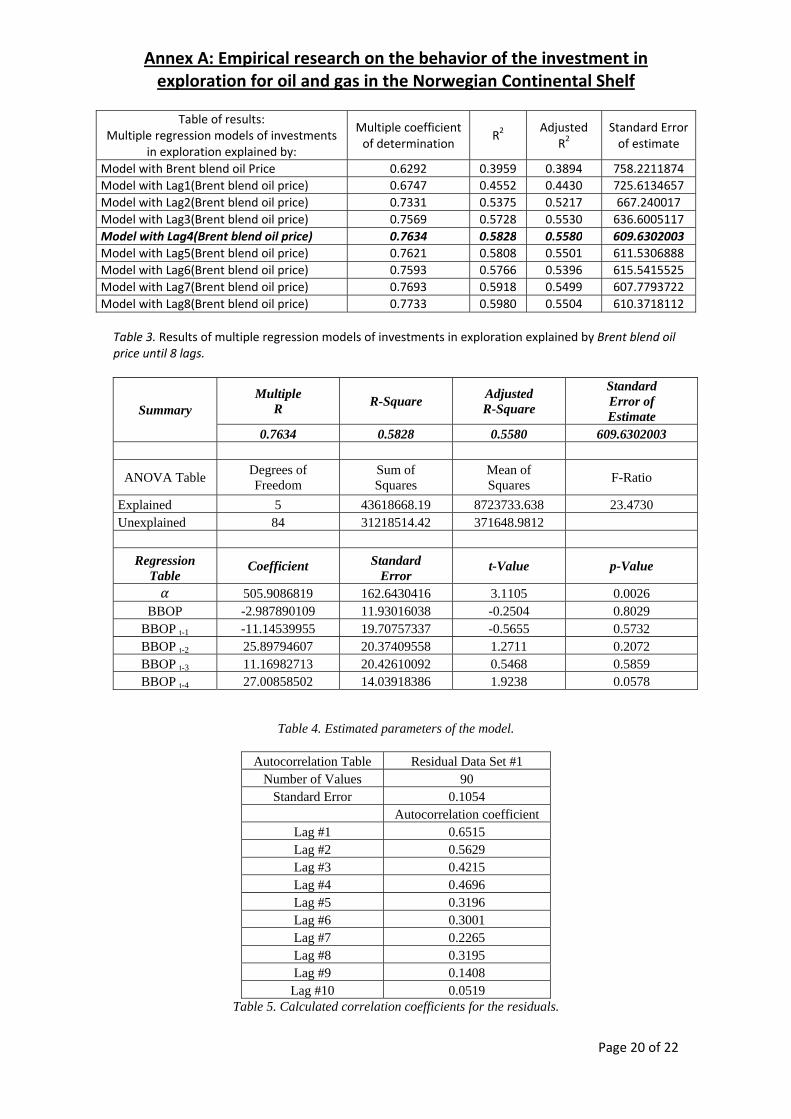
Annex A: Empirical research on the behavior of the investment in exploration for oil and gas in the Norwegian Continental Shelf
Page 20 of 22
Table of results:
Multiple regression models of investments in exploration explained by:
Multiple coefficient of determination
R2 Adjusted
R2 Standard Error of estimate
Model with Brent blend oil Price 0.6292 0.3959 0.3894 758.2211874Model with Lag1(Brent blend oil price) 0.6747 0.4552 0.4430 725.6134657Model with Lag2(Brent blend oil price) 0.7331 0.5375 0.5217 667.240017Model with Lag3(Brent blend oil price) 0.7569 0.5728 0.5530 636.6005117Model with Lag4(Brent blend oil price) 0.7634 0.5828 0.5580 609.6302003Model with Lag5(Brent blend oil price) 0.7621 0.5808 0.5501 611.5306888Model with Lag6(Brent blend oil price) 0.7593 0.5766 0.5396 615.5415525Model with Lag7(Brent blend oil price) 0.7693 0.5918 0.5499 607.7793722Model with Lag8(Brent blend oil price) 0.7733 0.5980 0.5504 610.3718112 Table 3. Results of multiple regression models of investments in exploration explained by Brent blend oil price until 8 lags.
Summary Multiple
R R-Square Adjusted R-Square
Standard Error of Estimate
0.7634 0.5828 0.5580 609.6302003
ANOVA Table Degrees of Freedom
Sum of Squares
Mean of Squares F-Ratio
Explained 5 43618668.19 8723733.638 23.4730 Unexplained 84 31218514.42 371648.9812
Regression Table
Coefficient Standard Error
t-Value p-Value
505.9086819 162.6430416 3.1105 0.0026 BBOP -2.987890109 11.93016038 -0.2504 0.8029
BBOP t-1 -11.14539955 19.70757337 -0.5655 0.5732 BBOP t-2 25.89794607 20.37409558 1.2711 0.2072 BBOP t-3 11.16982713 20.42610092 0.5468 0.5859 BBOP t-4 27.00858502 14.03918386 1.9238 0.0578
Table 4. Estimated parameters of the model.
Table 5. Calculated correlation coefficients for the residuals.
Autocorrelation Table Residual Data Set #1 Number of Values 90
Standard Error 0.1054 Autocorrelation coefficient
Lag #1 0.6515 Lag #2 0.5629 Lag #3 0.4215 Lag #4 0.4696 Lag #5 0.3196 Lag #6 0.3001 Lag #7 0.2265 Lag #8 0.3195 Lag #9 0.1408
Lag #10 0.0519
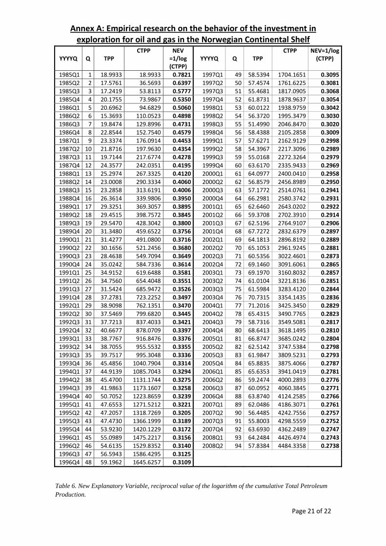
Annex A: Empirical research on the behavior of the investment in exploration for oil and gas in the Norwegian Continental Shelf
Page 21 of 22
YYYYQ Q TPP CTPP NEV
=1/log (CTPP)
YYYYQ Q TPP CTPP NEV=1/log
(CTPP)
1985Q1 1 18.9933 18.9933 0.7821 1997Q1 49 58.5394 1704.1651 0.30951985Q2 2 17.5761 36.5693 0.6397 1997Q2 50 57.4574 1761.6225 0.30811985Q3 3 17.2419 53.8113 0.5777 1997Q3 51 55.4681 1817.0905 0.30681985Q4 4 20.1755 73.9867 0.5350 1997Q4 52 61.8731 1878.9637 0.30541986Q1 5 20.6962 94.6829 0.5060 1998Q1 53 60.0122 1938.9759 0.30421986Q2 6 15.3693 110.0523 0.4898 1998Q2 54 56.3720 1995.3479 0.30301986Q3 7 19.8474 129.8996 0.4731 1998Q3 55 51.4990 2046.8470 0.30201986Q4 8 22.8544 152.7540 0.4579 1998Q4 56 58.4388 2105.2858 0.30091987Q1 9 23.3374 176.0914 0.4453 1999Q1 57 57.6271 2162.9129 0.29981987Q2 10 21.8716 197.9630 0.4354 1999Q2 58 54.3967 2217.3096 0.29891987Q3 11 19.7144 217.6774 0.4278 1999Q3 59 55.0168 2272.3264 0.29791987Q4 12 24.3577 242.0351 0.4195 1999Q4 60 63.6170 2335.9433 0.29691988Q1 13 25.2974 267.3325 0.4120 2000Q1 61 64.0977 2400.0410 0.29581988Q2 14 23.0008 290.3334 0.4060 2000Q2 62 56.8579 2456.8989 0.29501988Q3 15 23.2858 313.6191 0.4006 2000Q3 63 57.1772 2514.0761 0.29411988Q4 16 26.3614 339.9806 0.3950 2000Q4 64 66.2981 2580.3742 0.29311989Q1 17 29.3251 369.3057 0.3895 2001Q1 65 62.6460 2643.0202 0.29221989Q2 18 29.4515 398.7572 0.3845 2001Q2 66 59.3708 2702.3910 0.29141989Q3 19 29.5470 428.3042 0.3800 2001Q3 67 62.5196 2764.9107 0.29061989Q4 20 31.3480 459.6522 0.3756 2001Q4 68 67.7272 2832.6379 0.28971990Q1 21 31.4277 491.0800 0.3716 2002Q1 69 64.1813 2896.8192 0.28891990Q2 22 30.1656 521.2456 0.3680 2002Q2 70 65.1053 2961.9245 0.28811990Q3 23 28.4638 549.7094 0.3649 2002Q3 71 60.5356 3022.4601 0.28731990Q4 24 35.0242 584.7336 0.3614 2002Q4 72 69.1460 3091.6061 0.28651991Q1 25 34.9152 619.6488 0.3581 2003Q1 73 69.1970 3160.8032 0.28571991Q2 26 34.7560 654.4048 0.3551 2003Q2 74 61.0104 3221.8136 0.28511991Q3 27 31.5424 685.9472 0.3526 2003Q3 75 61.5984 3283.4120 0.28441991Q4 28 37.2781 723.2252 0.3497 2003Q4 76 70.7315 3354.1435 0.28361992Q1 29 38.9098 762.1351 0.3470 2004Q1 77 71.2016 3425.3450 0.28291992Q2 30 37.5469 799.6820 0.3445 2004Q2 78 65.4315 3490.7765 0.28231992Q3 31 37.7213 837.4033 0.3421 2004Q3 79 58.7316 3549.5081 0.28171992Q4 32 40.6677 878.0709 0.3397 2004Q4 80 68.6413 3618.1495 0.28101993Q1 33 38.7767 916.8476 0.3376 2005Q1 81 66.8747 3685.0242 0.28041993Q2 34 38.7055 955.5532 0.3355 2005Q2 82 62.5142 3747.5384 0.27981993Q3 35 39.7517 995.3048 0.3336 2005Q3 83 61.9847 3809.5231 0.27931993Q4 36 45.4856 1040.7904 0.3314 2005Q4 84 65.8835 3875.4066 0.27871994Q1 37 44.9139 1085.7043 0.3294 2006Q1 85 65.6353 3941.0419 0.27811994Q2 38 45.4700 1131.1744 0.3275 2006Q2 86 59.2474 4000.2893 0.27761994Q3 39 41.9863 1173.1607 0.3258 2006Q3 87 60.0952 4060.3845 0.27711994Q4 40 50.7052 1223.8659 0.3239 2006Q4 88 63.8740 4124.2585 0.27661995Q1 41 47.6553 1271.5212 0.3221 2007Q1 89 62.0486 4186.3071 0.27611995Q2 42 47.2057 1318.7269 0.3205 2007Q2 90 56.4485 4242.7556 0.27571995Q3 43 47.4730 1366.1999 0.3189 2007Q3 91 55.8003 4298.5559 0.27521995Q4 44 53.9230 1420.1229 0.3172 2007Q4 92 63.6930 4362.2489 0.27471996Q1 45 55.0989 1475.2217 0.3156 2008Q1 93 64.2484 4426.4974 0.27431996Q2 46 54.6135 1529.8352 0.3140 2008Q2 94 57.8384 4484.3358 0.27381996Q3 47 56.5943 1586.4295 0.31251996Q4 48 59.1962 1645.6257 0.3109
Table 6. New Explanatory Variable, reciprocal value of the logarithm of the cumulative Total Petroleum Production.
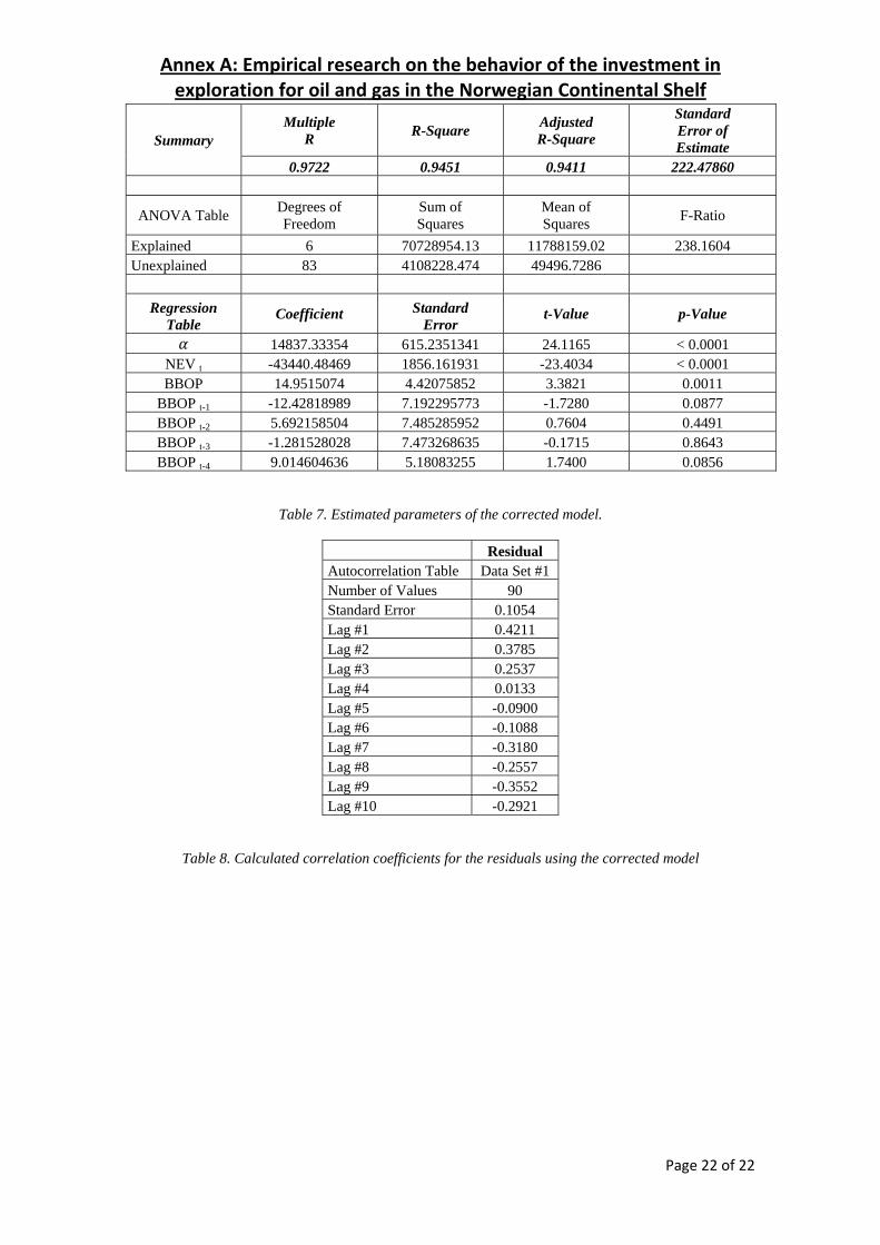
Annex A: Empirical research on the behavior of the investment in exploration for oil and gas in the Norwegian Continental Shelf
Page 22 of 22
Summary Multiple
R R-Square Adjusted R-Square
Standard Error of Estimate
0.9722 0.9451 0.9411 222.47860
ANOVA Table Degrees of Freedom
Sum of Squares
Mean of Squares F-Ratio
Explained 6 70728954.13 11788159.02 238.1604 Unexplained 83 4108228.474 49496.7286
Regression Table
Coefficient Standard Error
t-Value p-Value
14837.33354 615.2351341 24.1165 < 0.0001 NEV t -43440.48469 1856.161931 -23.4034 < 0.0001 BBOP 14.9515074 4.42075852 3.3821 0.0011
BBOP t-1 -12.42818989 7.192295773 -1.7280 0.0877 BBOP t-2 5.692158504 7.485285952 0.7604 0.4491 BBOP t-3 -1.281528028 7.473268635 -0.1715 0.8643 BBOP t-4 9.014604636 5.18083255 1.7400 0.0856
Table 7. Estimated parameters of the corrected model.
Residual Autocorrelation Table Data Set #1 Number of Values 90 Standard Error 0.1054 Lag #1 0.4211 Lag #2 0.3785 Lag #3 0.2537 Lag #4 0.0133 Lag #5 -0.0900 Lag #6 -0.1088 Lag #7 -0.3180 Lag #8 -0.2557 Lag #9 -0.3552 Lag #10 -0.2921
Table 8. Calculated correlation coefficients for the residuals using the corrected model
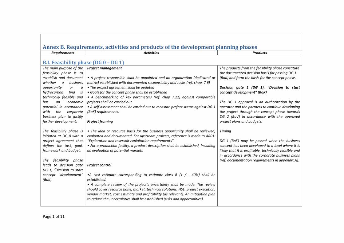
Page 1 of 11
Annex B. Requirements, activities and products of the development planning phases Requirements Activities Products
B.I. Feasibility phase (DG 0 – DG 1) The main purpose of the feasibility phase is to establish and document whether a business opportunity or a hydrocarbon find is technically feasible and has an economic potential in accordance with the corporate business plan to justify further development. The feasibility phase is initiated at DG 0 with a project agreement that defines the task, goal, framework and budget. The feasibility phase leads to decision gate DG 1, “Decision to start concept development” (BoK).
Project management • A project responsible shall be appointed and an organization (dedicated or matrix) established with documented responsibility and tasks (ref. chap. 7.6) • The project agreement shall be updated • Goals for the concept phase shall be established • A benchmarking of key parameters (ref. chap 7.21) against comparable projects shall be carried out • A self‐assessment shall be carried out to measure project status against DG 1 (BoK) requirements. Project framing • The idea or resource basis for the business opportunity shall be reviewed, evaluated and documented. For upstream projects, reference is made to AR01: “Exploration and reservoir exploitation requirements”. • For a production facility, a product description shall be established, including an evaluation of potential markets
Project control •A cost estimate corresponding to estimate class B (+ / ‐ 40%) shall be established. • A complete review of the project’s uncertainty shall be made. The review should cover resource basis, market, technical solutions, HSE, project execution, vendor market, cost estimate and profitability (as relevant). An mitigation plan to reduce the uncertainties shall be established (risks and opportunities)
The products from the feasibility phase constitute the documented decision basis for passing DG 1 (BoK) and form the basis for the concept phase. Decision gate 1 (DG 1), "Decision to start concept development" (BoK) The DG 1 approval is an authorization by the operator and the partners to continue developing the project through the concept phase towards DG 2 (BoV) in accordance with the approved project plans and budgets.
Timing
DG 1 (BoK) may be passed when the business concept has been developed to a level where it is likely that it is profitable, technically feasible and in accordance with the corporate business plans (ref. documentation requirements in appendix A).
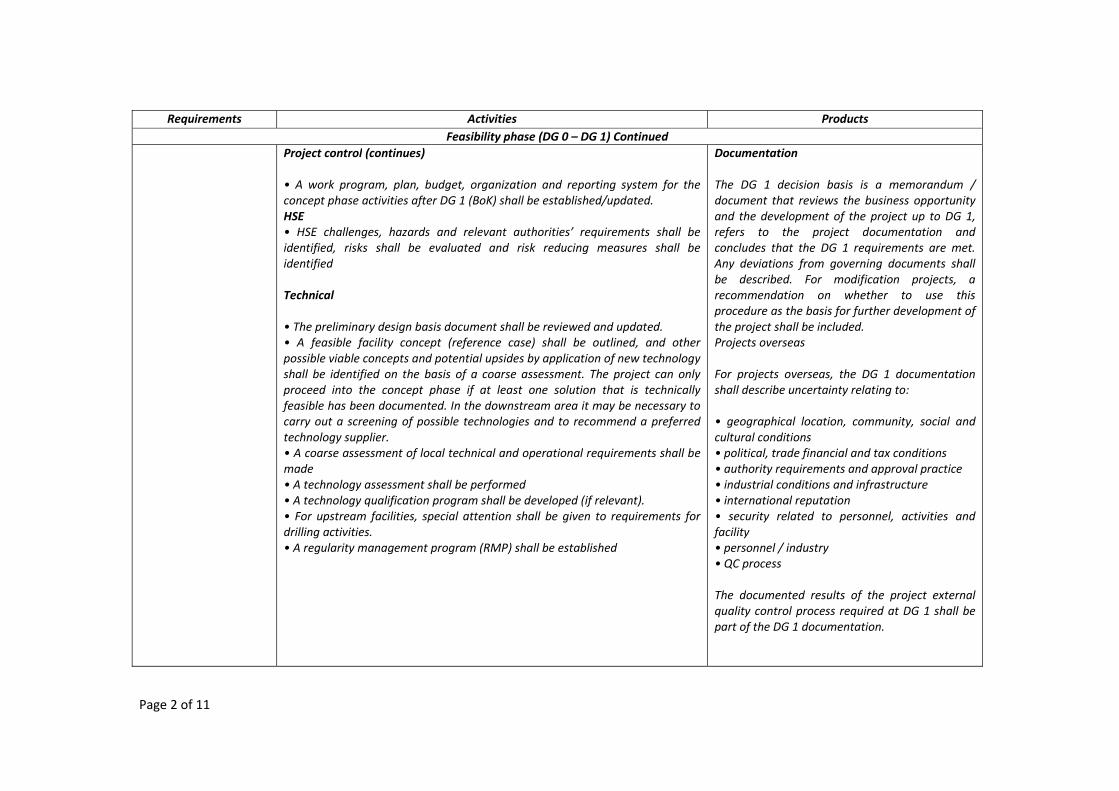
Page 2 of 11
Requirements Activities ProductsFeasibility phase (DG 0 – DG 1) Continued
Project control (continues) • A work program, plan, budget, organization and reporting system for the concept phase activities after DG 1 (BoK) shall be established/updated. HSE • HSE challenges, hazards and relevant authorities’ requirements shall be identified, risks shall be evaluated and risk reducing measures shall be identified Technical • The preliminary design basis document shall be reviewed and updated. • A feasible facility concept (reference case) shall be outlined, and other possible viable concepts and potential upsides by application of new technology shall be identified on the basis of a coarse assessment. The project can only proceed into the concept phase if at least one solution that is technically feasible has been documented. In the downstream area it may be necessary to carry out a screening of possible technologies and to recommend a preferred technology supplier. • A coarse assessment of local technical and operational requirements shall be made • A technology assessment shall be performed • A technology qualification program shall be developed (if relevant). • For upstream facilities, special attention shall be given to requirements for drilling activities. • A regularity management program (RMP) shall be established
Documentation
The DG 1 decision basis is a memorandum / document that reviews the business opportunity and the development of the project up to DG 1, refers to the project documentation and concludes that the DG 1 requirements are met. Any deviations from governing documents shall be described. For modification projects, a recommendation on whether to use this procedure as the basis for further development of the project shall be included. Projects overseas For projects overseas, the DG 1 documentation shall describe uncertainty relating to: • geographical location, community, social and cultural conditions • political, trade financial and tax conditions • authority requirements and approval practice • industrial conditions and infrastructure • international reputation • security related to personnel, activities and facility • personnel / industry • QC process The documented results of the project external quality control process required at DG 1 shall be part of the DG 1 documentation.
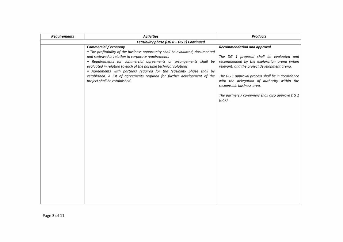
Page 3 of 11
Requirements Activities ProductsFeasibility phase (DG 0 – DG 1) Continued
Commercial / economy• The profitability of the business opportunity shall be evaluated, documented and reviewed in relation to corporate requirements • Requirements for commercial agreements or arrangements shall be evaluated in relation to each of the possible technical solutions • Agreements with partners required for the feasibility phase shall be established. A list of agreements required for further development of the project shall be established.
Recommendation and approval The DG 1 proposal shall be evaluated and recommended by the exploration arena (when relevant) and the project development arena. The DG 1 approval process shall be in accordance with the delegation of authority within the responsible business area. The partners / co‐owners shall also approve DG 1 (BoK).
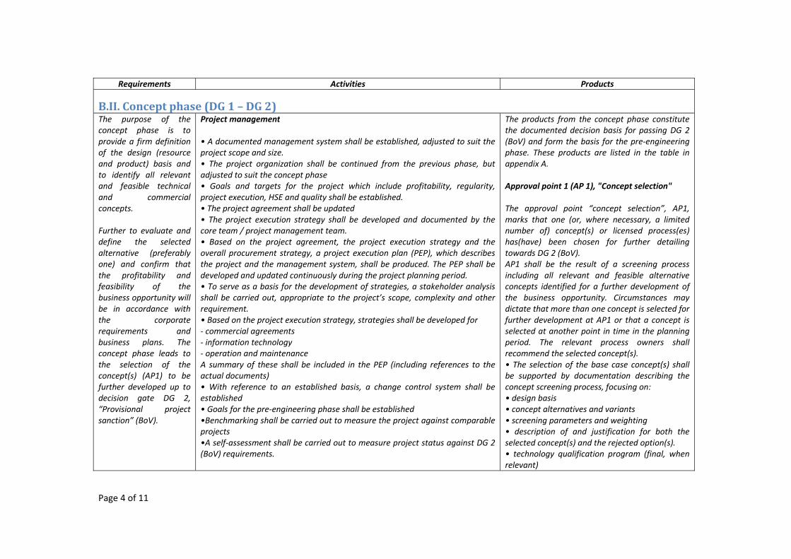
Page 4 of 11
Requirements Activities Products
B.II. Concept phase (DG 1 – DG 2) The purpose of the concept phase is to provide a firm definition of the design (resource and product) basis and to identify all relevant and feasible technical and commercial concepts. Further to evaluate and define the selected alternative (preferably one) and confirm that the profitability and feasibility of the business opportunity will be in accordance with the corporate requirements and business plans. The concept phase leads to the selection of the concept(s) (AP1) to be further developed up to decision gate DG 2, “Provisional project sanction” (BoV).
Project management • A documented management system shall be established, adjusted to suit the project scope and size. • The project organization shall be continued from the previous phase, but adjusted to suit the concept phase • Goals and targets for the project which include profitability, regularity, project execution, HSE and quality shall be established. • The project agreement shall be updated • The project execution strategy shall be developed and documented by the core team / project management team. • Based on the project agreement, the project execution strategy and the overall procurement strategy, a project execution plan (PEP), which describes the project and the management system, shall be produced. The PEP shall be developed and updated continuously during the project planning period. • To serve as a basis for the development of strategies, a stakeholder analysis shall be carried out, appropriate to the project’s scope, complexity and other requirement. • Based on the project execution strategy, strategies shall be developed for ‐ commercial agreements ‐ information technology ‐ operation and maintenance A summary of these shall be included in the PEP (including references to the actual documents) • With reference to an established basis, a change control system shall be established • Goals for the pre‐engineering phase shall be established •Benchmarking shall be carried out to measure the project against comparable projects •A self‐assessment shall be carried out to measure project status against DG 2 (BoV) requirements.
The products from the concept phase constitute the documented decision basis for passing DG 2 (BoV) and form the basis for the pre‐engineering phase. These products are listed in the table in appendix A. Approval point 1 (AP 1), "Concept selection" The approval point “concept selection”, AP1, marks that one (or, where necessary, a limited number of) concept(s) or licensed process(es) has(have) been chosen for further detailing towards DG 2 (BoV). AP1 shall be the result of a screening process including all relevant and feasible alternative concepts identified for a further development of the business opportunity. Circumstances may dictate that more than one concept is selected for further development at AP1 or that a concept is selected at another point in time in the planning period. The relevant process owners shall recommend the selected concept(s). • The selection of the base case concept(s) shall be supported by documentation describing the concept screening process, focusing on: • design basis • concept alternatives and variants • screening parameters and weighting • description of and justification for both the selected concept(s) and the rejected option(s). • technology qualification program (final, when relevant)
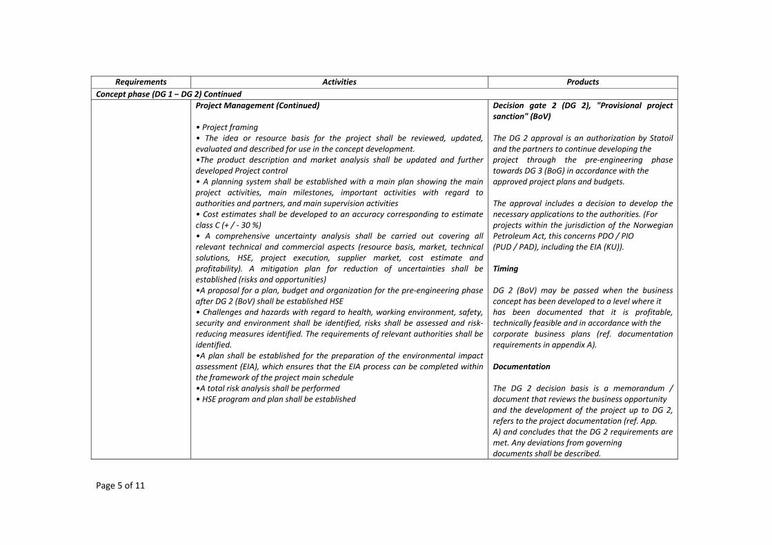
Page 5 of 11
Requirements Activities ProductsConcept phase (DG 1 – DG 2) Continued Project Management (Continued)
• Project framing • The idea or resource basis for the project shall be reviewed, updated, evaluated and described for use in the concept development. •The product description and market analysis shall be updated and further developed Project control • A planning system shall be established with a main plan showing the main project activities, main milestones, important activities with regard to authorities and partners, and main supervision activities • Cost estimates shall be developed to an accuracy corresponding to estimate class C (+ / ‐ 30 %) • A comprehensive uncertainty analysis shall be carried out covering all relevant technical and commercial aspects (resource basis, market, technical solutions, HSE, project execution, supplier market, cost estimate and profitability). A mitigation plan for reduction of uncertainties shall be established (risks and opportunities) •A proposal for a plan, budget and organization for the pre‐engineering phase after DG 2 (BoV) shall be established HSE • Challenges and hazards with regard to health, working environment, safety, security and environment shall be identified, risks shall be assessed and risk‐reducing measures identified. The requirements of relevant authorities shall be identified. •A plan shall be established for the preparation of the environmental impact assessment (EIA), which ensures that the EIA process can be completed within the framework of the project main schedule •A total risk analysis shall be performed • HSE program and plan shall be established
Decision gate 2 (DG 2), "Provisional project sanction" (BoV) The DG 2 approval is an authorization by Statoil and the partners to continue developing the project through the pre‐engineering phase towards DG 3 (BoG) in accordance with the approved project plans and budgets. The approval includes a decision to develop the necessary applications to the authorities. (For projects within the jurisdiction of the Norwegian Petroleum Act, this concerns PDO / PIO (PUD / PAD), including the EIA (KU)). Timing DG 2 (BoV) may be passed when the business concept has been developed to a level where it has been documented that it is profitable, technically feasible and in accordance with the corporate business plans (ref. documentation requirements in appendix A). Documentation The DG 2 decision basis is a memorandum / document that reviews the business opportunity and the development of the project up to DG 2, refers to the project documentation (ref. App. A) and concludes that the DG 2 requirements are met. Any deviations from governing documents shall be described.
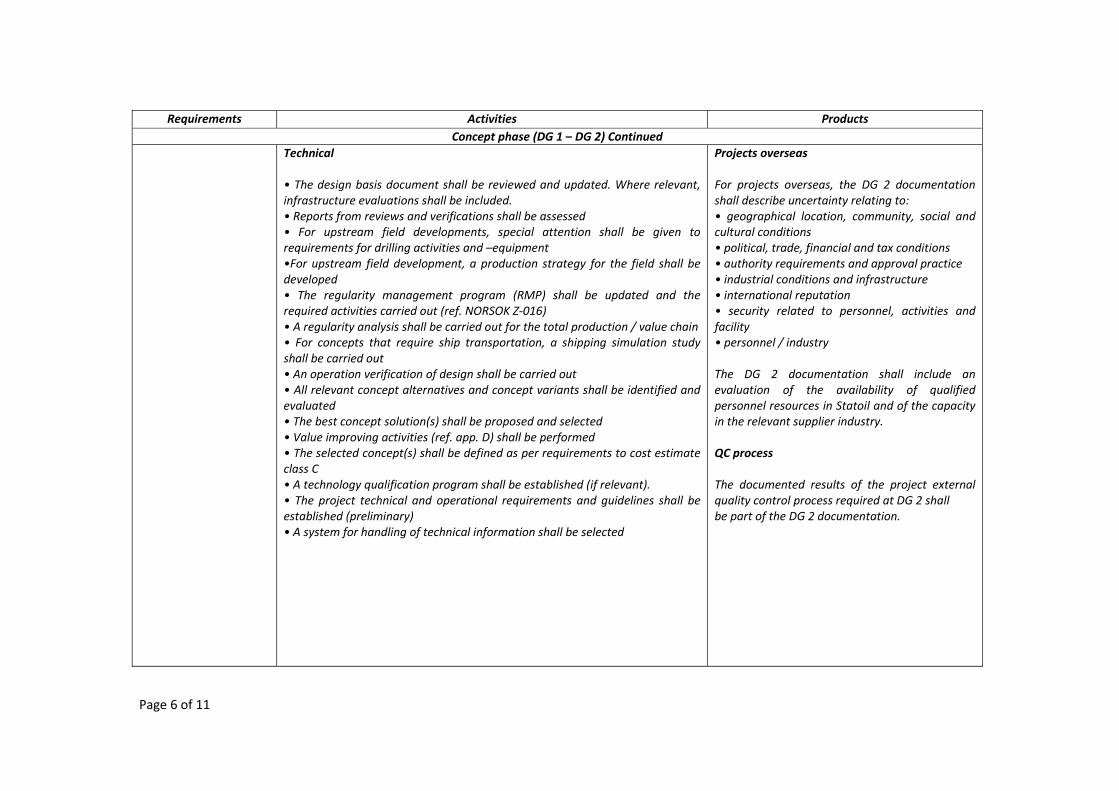
Page 6 of 11
Requirements Activities ProductsConcept phase (DG 1 – DG 2) Continued
Technical • The design basis document shall be reviewed and updated. Where relevant, infrastructure evaluations shall be included. • Reports from reviews and verifications shall be assessed • For upstream field developments, special attention shall be given to requirements for drilling activities and –equipment •For upstream field development, a production strategy for the field shall be developed • The regularity management program (RMP) shall be updated and the required activities carried out (ref. NORSOK Z‐016) • A regularity analysis shall be carried out for the total production / value chain • For concepts that require ship transportation, a shipping simulation study shall be carried out • An operation verification of design shall be carried out • All relevant concept alternatives and concept variants shall be identified and evaluated • The best concept solution(s) shall be proposed and selected • Value improving activities (ref. app. D) shall be performed • The selected concept(s) shall be defined as per requirements to cost estimate class C • A technology qualification program shall be established (if relevant). • The project technical and operational requirements and guidelines shall be established (preliminary) • A system for handling of technical information shall be selected
Projects overseas For projects overseas, the DG 2 documentation shall describe uncertainty relating to: • geographical location, community, social and cultural conditions • political, trade, financial and tax conditions • authority requirements and approval practice • industrial conditions and infrastructure • international reputation • security related to personnel, activities and facility • personnel / industry The DG 2 documentation shall include an evaluation of the availability of qualified personnel resources in Statoil and of the capacity in the relevant supplier industry. QC process The documented results of the project external quality control process required at DG 2 shall be part of the DG 2 documentation.
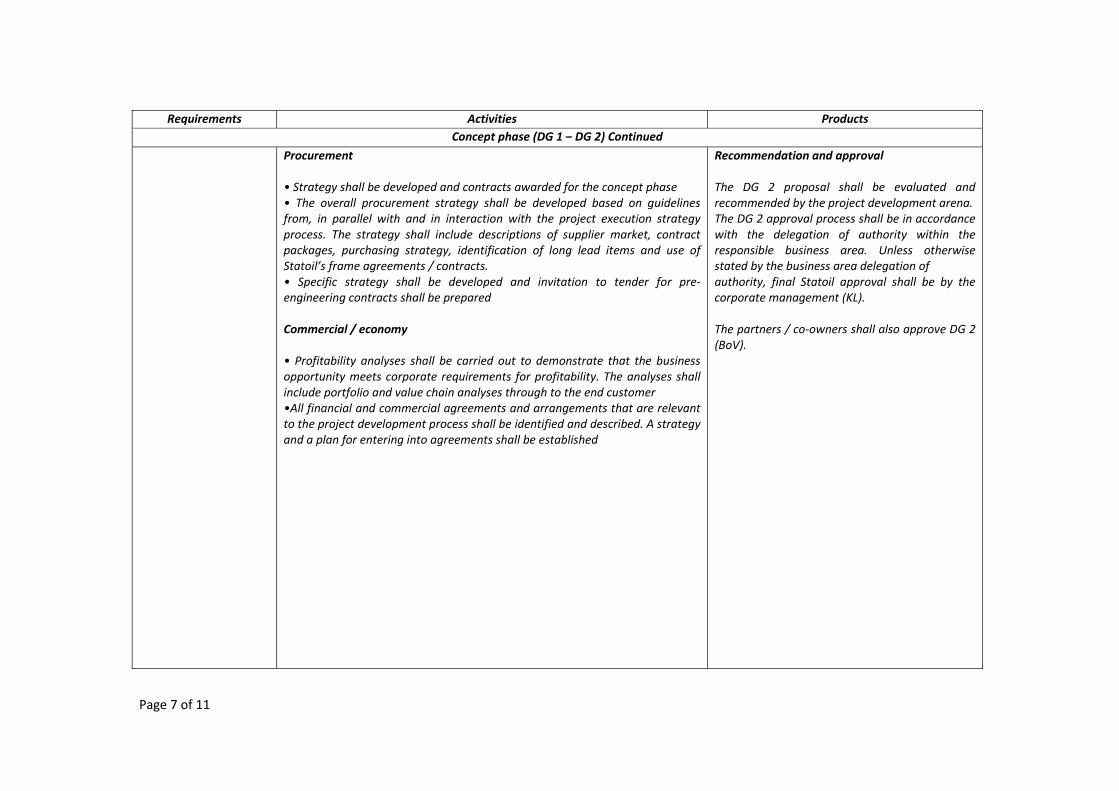
Page 7 of 11
Requirements Activities ProductsConcept phase (DG 1 – DG 2) Continued
Procurement • Strategy shall be developed and contracts awarded for the concept phase • The overall procurement strategy shall be developed based on guidelines from, in parallel with and in interaction with the project execution strategy process. The strategy shall include descriptions of supplier market, contract packages, purchasing strategy, identification of long lead items and use of Statoil’s frame agreements / contracts. • Specific strategy shall be developed and invitation to tender for pre‐engineering contracts shall be prepared Commercial / economy
• Profitability analyses shall be carried out to demonstrate that the business opportunity meets corporate requirements for profitability. The analyses shall include portfolio and value chain analyses through to the end customer •All financial and commercial agreements and arrangements that are relevant to the project development process shall be identified and described. A strategy and a plan for entering into agreements shall be established
Recommendation and approval The DG 2 proposal shall be evaluated and recommended by the project development arena. The DG 2 approval process shall be in accordance with the delegation of authority within the responsible business area. Unless otherwise stated by the business area delegation of authority, final Statoil approval shall be by the corporate management (KL). The partners / co‐owners shall also approve DG 2 (BoV).
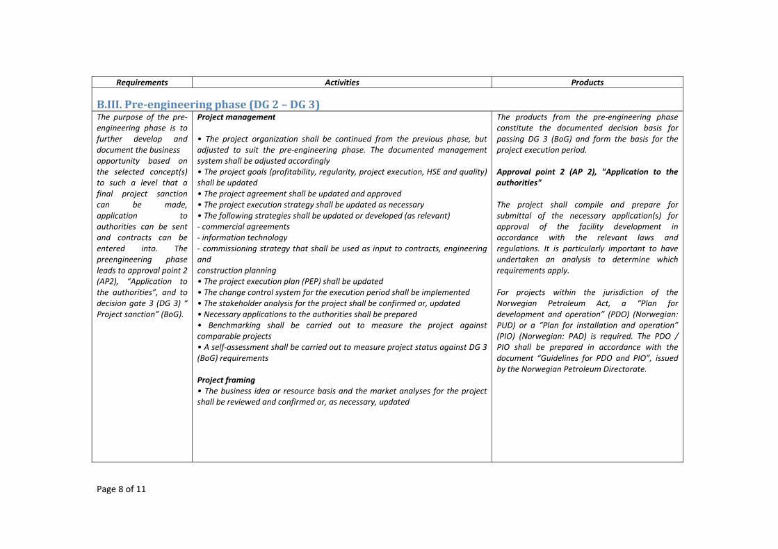
Page 8 of 11
Requirements Activities Products
B.III. Preengineering phase (DG 2 – DG 3) The purpose of the pre‐engineering phase is to further develop and document the business opportunity based on the selected concept(s) to such a level that a final project sanction can be made, application to authorities can be sent and contracts can be entered into. The preengineering phase leads to approval point 2 (AP2), “Application to the authorities”, and to decision gate 3 (DG 3) “ Project sanction” (BoG).
Project management • The project organization shall be continued from the previous phase, but adjusted to suit the pre‐engineering phase. The documented management system shall be adjusted accordingly • The project goals (profitability, regularity, project execution, HSE and quality) shall be updated • The project agreement shall be updated and approved • The project execution strategy shall be updated as necessary • The following strategies shall be updated or developed (as relevant) ‐ commercial agreements ‐ information technology ‐ commissioning strategy that shall be used as input to contracts, engineering and construction planning • The project execution plan (PEP) shall be updated • The change control system for the execution period shall be implemented • The stakeholder analysis for the project shall be confirmed or, updated • Necessary applications to the authorities shall be prepared • Benchmarking shall be carried out to measure the project against comparable projects • A self‐assessment shall be carried out to measure project status against DG 3 (BoG) requirements Project framing • The business idea or resource basis and the market analyses for the project shall be reviewed and confirmed or, as necessary, updated
The products from the pre‐engineering phase constitute the documented decision basis for passing DG 3 (BoG) and form the basis for the project execution period. Approval point 2 (AP 2), "Application to the authorities" The project shall compile and prepare for submittal of the necessary application(s) for approval of the facility development in accordance with the relevant laws and regulations. It is particularly important to have undertaken an analysis to determine which requirements apply. For projects within the jurisdiction of the Norwegian Petroleum Act, a “Plan for development and operation” (PDO) (Norwegian: PUD) or a “Plan for installation and operation” (PIO) (Norwegian: PAD) is required. The PDO / PIO shall be prepared in accordance with the document “Guidelines for PDO and PIO”, issued by the Norwegian Petroleum Directorate.
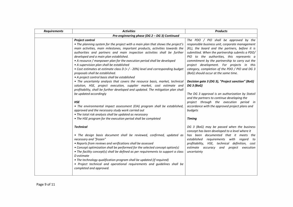
Page 9 of 11
Requirements Activities ProductsPre‐enginnering phase (DG 2 – DG 3) Continued
Project control• The planning system for the project with a main plan that shows the project’s main activities, main milestones, important products, activities towards the authorities and partners and main inspection activities shall be further developed and a main plan established. • A resource / manpower plan for the execution period shall be developed • A supervision plan shall be established • Cost estimates at estimate class D (+ / ‐ 20%) level and corresponding budget proposals shall be established. • A project control basis shall be established • The uncertainty analysis that covers the resource basis, market, technical solution, HSE, project execution, supplier market, cost estimate and profitability, shall be further developed and updated. The mitigation plan shall be updated accordingly HSE • The environmental impact assessment (EIA) program shall be established, approved and the necessary study work carried out • The total risk analysis shall be updated as necessary • The HSE program for the execution period shall be completed Technical • The design basis document shall be reviewed, confirmed, updated as necessary and "frozen" • Reports from reviews and verifications shall be assessed • Concept optimization shall be performed for the selected concept option(s) • The facility concept(s) shall be defined as per requirements to support a class D estimate • The technology qualification program shall be updated (if required) • Project technical and operational requirements and guidelines shall be completed and approved.
The PDO / PIO shall be approved by the responsible business unit, corporate management (KL), the board and the partners, before it is submitted. When the partnership submits a PDO/ PIO to the authorities, this represents a commitment by the partnership to carry out the project development. For projects in this category, completion of the PDO / PIO and DG 3 (BoG) should occur at the same time. Decision gate 3 (DG 3), "Project sanction" (BoG) DG 3 (BoG) The DG 3 approval is an authorization by Statoil and the partners to continue developing the project through the execution period in accordance with the approved project plans and budgets Timing DG 3 (BoG) may be passed when the business concept has been developed to a level where it has been documented that it meets the established requirements with regard to profitability, HSE, technical definition, cost estimate accuracy and project execution uncertainty
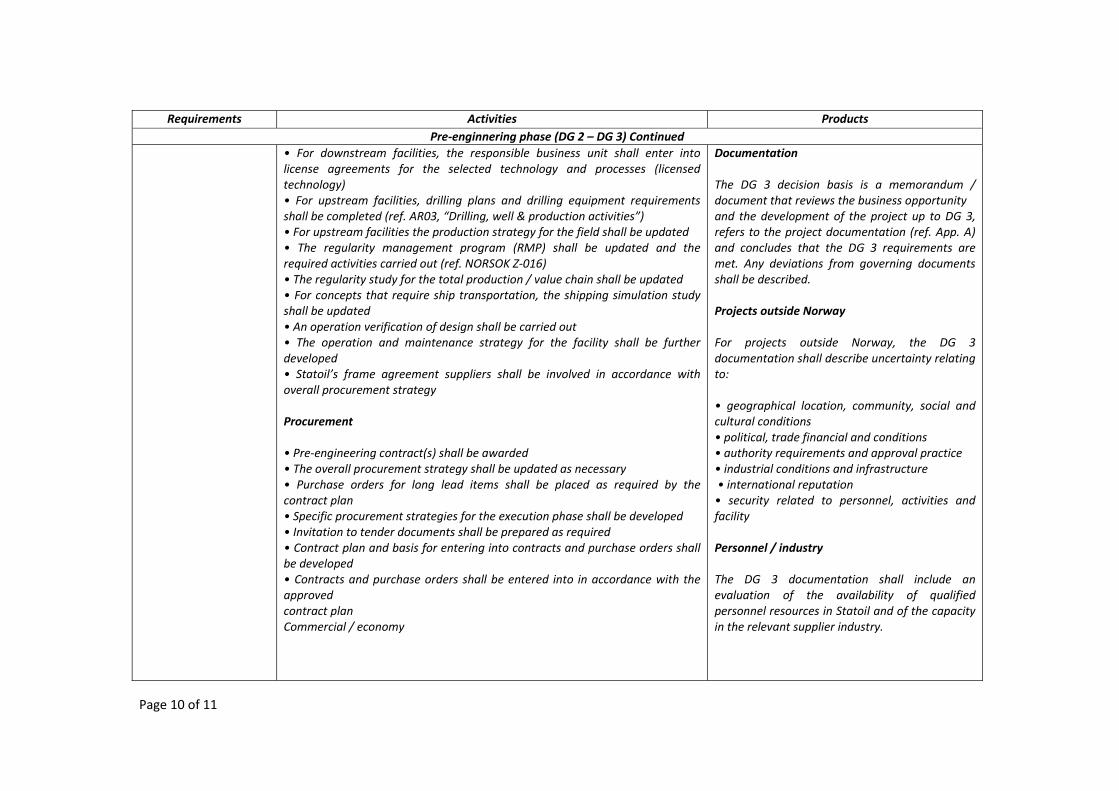
Page 10 of 11
Requirements Activities ProductsPre‐enginnering phase (DG 2 – DG 3) Continued
• For downstream facilities, the responsible business unit shall enter into license agreements for the selected technology and processes (licensed technology) • For upstream facilities, drilling plans and drilling equipment requirements shall be completed (ref. AR03, “Drilling, well & production activities”) • For upstream facilities the production strategy for the field shall be updated • Τhe regularity management program (RMP) shall be updated and the required activities carried out (ref. NORSOK Z‐016) • The regularity study for the total production / value chain shall be updated • For concepts that require ship transportation, the shipping simulation study shall be updated • An operation verification of design shall be carried out • The operation and maintenance strategy for the facility shall be further developed • Statoil’s frame agreement suppliers shall be involved in accordance with overall procurement strategy Procurement • Pre‐engineering contract(s) shall be awarded • The overall procurement strategy shall be updated as necessary • Purchase orders for long lead items shall be placed as required by the contract plan • Specific procurement strategies for the execution phase shall be developed • Invitation to tender documents shall be prepared as required • Contract plan and basis for entering into contracts and purchase orders shall be developed • Contracts and purchase orders shall be entered into in accordance with the approved contract plan Commercial / economy
Documentation The DG 3 decision basis is a memorandum / document that reviews the business opportunity and the development of the project up to DG 3, refers to the project documentation (ref. App. A) and concludes that the DG 3 requirements are met. Any deviations from governing documents shall be described. Projects outside Norway For projects outside Norway, the DG 3 documentation shall describe uncertainty relating to: • geographical location, community, social and cultural conditions • political, trade financial and conditions • authority requirements and approval practice • industrial conditions and infrastructure • international reputation • security related to personnel, activities and facility
Personnel / industry The DG 3 documentation shall include an evaluation of the availability of qualified personnel resources in Statoil and of the capacity in the relevant supplier industry.
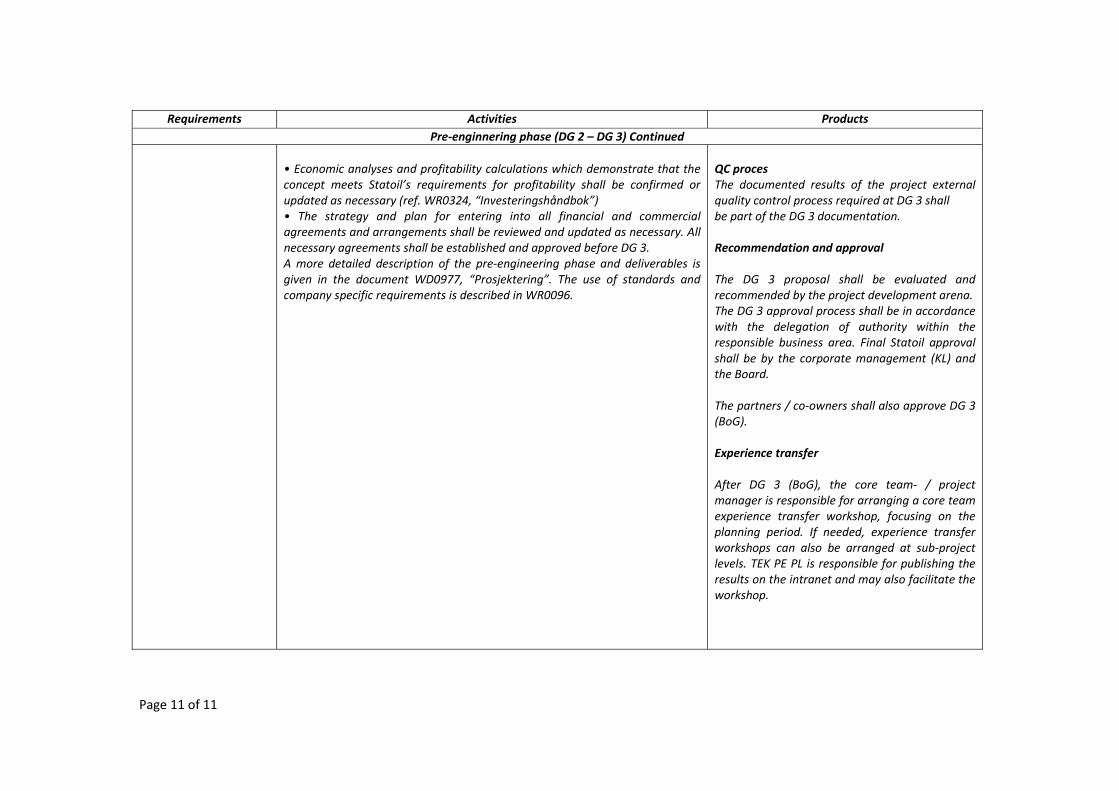
Page 11 of 11
Requirements Activities ProductsPre‐enginnering phase (DG 2 – DG 3) Continued
• Economic analyses and profitability calculations which demonstrate that the concept meets Statoil’s requirements for profitability shall be confirmed or updated as necessary (ref. WR0324, “Investeringshåndbok”) • The strategy and plan for entering into all financial and commercial agreements and arrangements shall be reviewed and updated as necessary. All necessary agreements shall be established and approved before DG 3. A more detailed description of the pre‐engineering phase and deliverables is given in the document WD0977, “Prosjektering”. The use of standards and company specific requirements is described in WR0096.
QC proces The documented results of the project external quality control process required at DG 3 shall be part of the DG 3 documentation. Recommendation and approval The DG 3 proposal shall be evaluated and recommended by the project development arena. The DG 3 approval process shall be in accordance with the delegation of authority within the responsible business area. Final Statoil approval shall be by the corporate management (KL) and the Board. The partners / co‐owners shall also approve DG 3 (BoG). Experience transfer After DG 3 (BoG), the core team‐ / project manager is responsible for arranging a core team experience transfer workshop, focusing on the planning period. If needed, experience transfer workshops can also be arranged at sub‐project levels. TEK PE PL is responsible for publishing the results on the intranet and may also facilitate the workshop.
Annex C: Field Development Examples
C.I. Subsea tieback to shore: Ormen Lange, Norway. Name of the project: Ormen Lange Operator: Shell Water Depth: 850 m / 2,805 ft Region: Europe ‐ North Sea Country: Norway Project Description Discovered in 1997, Ormen Lange is Europe's third‐largest gas field with estimated recoverable reserves of 14 Tcf (397 Bcm) of natural gas. Located on the Norwegian Continental Shelf, 75 miles (120 kilometers) northwest of Kristiansund, Norway, in the Norwegian Sea, Ormen Lange reaches 25 miles (40 kilometers) by up to 6 miles (10 kilometers). Water depths for the field range from 2,625 to 3,609 feet (800 to 1,100 meters), and hydrocarbons are located another 9,843 feet (3,000 meters) below the surface. Partners in the field include Petoro with 36.48%, StatoilHydro with 28.91%, Shell with 17.04%, Dong with 10.34% and ExxonMobil with 7.23%. Like its development, Ormen Lange boasts a multiphase operatorship. StatoilHydro served as the field's operator during the first phase of development from 1999 through production start‐up in 2007. Shell took over operatorship for the production phase of the field, including the second phase of development. Overcoming Challenges There were a number of challenges that had to be overcome to bring natural gas from Ormen Lange to market. First of all, the field is in environmentally unfriendly waters. Both temperatures and strong currents sought to stop field development in its tracks. Water temperatures on the seafloor stay below freezing, and especially strong currents in the area threaten field facilities. Additionally, a mountainously uneven sea floor made for difficult subsea development. Despite these difficulties, designers devised a multiphase completely subsea field development plan, including the world's longest subsea pipeline. Submitted to Norwegian authorities on Dec. 4, 2003, the field development plan was approved on April 2, 2004. Field Development: Phase I At an estimated cost of US $8 billion (NOK 50 billion), the first phase of development included two 1,268‐ton (1,150‐tonne) subsea templates, as well as pipelines to shore and an onshore gas processing plant. Each subsea template holds slots for eight wells, which are hooked up to the templates via a subsea manifold. FMC was awarded the US $160 million (NOK 1 billion) contract to engineer, procure, fabricate and test the subsea production system, which consisted of the two subsea templates with manifolds, eight xmas trees, control systems, an intervention system, tie‐in tools, end terminations and Tee's for the pipelines. The contract also included options for additional xmas trees and control systems. Measuring 144 feet (44 meters) long by 108 feet (33 meters) wide and 49 feet (15 meters) wide, the subsea templates were installed by Hreema's Thialf crane barge using sound signals produced by subsea acoustic
transmitters. Positioned 2.2 miles (3.6 kilometers) away from each other, the subsea templates are in waters measuring 2,789 feet (850 meters). Additionally, a 386‐ton (350‐tonne) pipeline connection box was installed 164 feet (50 meters) away from the templates. Gas, condensate and water produced from the templates are transported through two 75‐mile (120‐kilometer), 30‐inch‐diameter multiphase flowlines up the Eggkanten embankment to the gas plant Nyhamna onshore the western coast of Norway. Saipem was awarded the US $105 million (NOK 660 million) pipeline installation contract, which included tie‐in operations. After installation of the subsea equipment, development drilling for the first phase of development was performed by the West Navigator drillship. The largest deepwater wells in the world at the time, Smedvig completed the US $167 million (NOK 1.17 billion) drilling contract over a two‐year period. Innovative Solutions To overcome icy water temperatures on the seafloor, Vetco Aibel was awarded the US $96 million (NOK 600 million) contract to engineer, procure and build a Monoethylen‐Glycol (MEG) regeneration system, which included a tank farm. MEG is used as anti‐freeze to prevent ice formations and plugs in the subsea production facility and pipelines. To counteract the strong currents in the deepwater of the Norwegian Sea, Van Oord ACZ was contracted to install 3 million tons (2.8 million tonnes) of rock on the seabed to protect and support pipelines and umbilicals from Ormen Lange to Nyhamna for a consideration of US $112 million (NOK 700 million). Production Production from Ormen Lange commenced on October 1, 2007. With daily rates expected to increase over the first couple of years, production rates for the first phase of development is 2.5 Bcf/d (70 MMcm/d) of natural gas and 50,000 barrels of condensate a day. Peak production is predicted for 2010. Natural gas is transported to market via the Gassco‐operated Langeled pipeline, the world's longest subsea transport pipeline, traversing 746 miles (1,200 kilometers to connect Nyhamna in Norway to Easingtown in the UK. Ensuring Long‐Term Production: Phase II The second phase of development on Ormen Lange includes the fabrication and installation of another two subsea templates. The first of them is under construction, and the fourth will be commissioned when necessary. In total, the four wellhead complexes on Ormen Lange will accommodate up to 24 wells. Both the Leiv Eiriksson semisub and the West Navigator drillship are employed on Ormen Lange for the second phase of development drilling. West Navigator was used through the summer of 2008 for development wells and to complete and make ready new wells for production. Leiv Eiriksson is drilling the planned monitoring well and several production wells through October 2009. Total costs for the second phase of development have not been released. Ormen Lange is expected to have a field life of 40 years. Offshore Compression Inevitably, as production decreases from Ormen Lange, so too will pressure. Once pressure can no longer drive produced gas to shore for processing, offshore compression will be required. There are two options for supplying offshore compression: a floating deepwater platform or a subsea compressor station.
While an offshore platform is more conventional, it is also more expensive than a subsea compressor. Two subsea compression pilot programs are being designed for use on the field. Aker Solutions was tapped to engineer, procure and fabricate a full‐size subsea compression station pilot, and Vetco Aibel was chosen to engineer, procure and construct a long step‐out power supply pilot. The subsea compressor will be located between the two original subsea templates in 2,789 feet (850 meters) of water. If chosen, the subsea compressor will be an industry first. At a cost of about US $ 401 million (NOK 2.5 billion), the subsea option is about half the cost of the offshore platform option. Testing of the two subsea compression pilots is expected to commence in 2009, and the best system will be chosen by 2011 with installation slated for 2015. Much of the decision will be based on reservoir properties.[Subsea IQ, 2010]
C.II. Subsea tieback to existing platform: Canyon Express, Gulf of Mexico U.S.A. Name of the project: Canyon Express Operator: Williams Water Depth: 2,346 m / 7,742 ft Region: N. America ‐ US GOM Country: US Project Description An innovative development project for its time, the Canyon Express allowed three different operators to bring three marginal gas fields into production through a subsea gas gathering system. Located in deepwater Gulf of Mexico, the Canyon Express traverses a number of blocks transporting gas from the Aconcagua, Camden Hills and King's Peak in the Mississippi Canyon. Although combined, the fields' boast a reserves reaching 900 Bcf (25 Bcm), none of them were commercially viable to be developed separately. Solving that problem, the Canyon Express project commingles gas from the three deepwater fields all located about 120 miles (193 kilometers) south of New Orleans, before transferring them to a third‐party shallow‐water production platform called the Canyon Station. Although the fields used to be operated by three different companies, all three fields, as well as the Canyon Express subsea development are now operated by ATP Oil & Gas. The Fields Located on Mississippi Canyon Block 348 in waters measuring 7,200 feet (2,195 meters) deep, Camden Hills was discovered in August 1999. Drilled by the Ocean Clipper semisub, the discovery well reached a total depth of 15,080 feet (4,596 meters) and encountered more than 200 feet (61 meters) of natural gas. Also discovered in 1999, the Aconcagua field is located on Mississippi Canyon Block 305 in approximately 7,000 feet (2,134 meters) of water. Drilled in March 2000, an appraisal well confirmed the discovery by intersecting more than 250 net feet (76 net meters) of gas. Situated in waters ranging in depth from 6,200 to 6,400 feet (1,890 to 1,951 meters), the King's Peak gas field spans Mississippi Canyon Blocks 217 and 173, as well as Desoto Canyon Blocks 133 and 177.
Canyon Express A subsea gas gathering system, Canyon Express was the longest and deepest subsea tie‐back at the time of its development. The $600 million project encompasses two 12‐inch‐diameter, 55‐mile‐long (88‐kilometer‐long) flowlines that transfer gas from the fields to a shallow‐water production platform 55 miles (88 kilometers) away. Ten subsea development wells are scattered across the fields and daisy‐chained together. Aconcagua has four wells, Camden Hills has two wells, and King's Peak has four wells. In order to monitor production at all times, each well is equipped with a wet gas flow meter. Additionally, each well is completed with two gravel‐packed intervals and an intelligent well completion system, allowing the wells to be produced independently or in a commingled state. Each of the wells delivers gas into one of the two flowlines that tie the wells back to the Canyon Station production platform. Canyon Express contains 32 individual pipeline segments, including all flowlines, supply lines, jumpers and umbilicals. Well tie‐in sleds installed as a part of the flowlines eliminated the need to install multiple well manifolds and infield flowlines. Wells are connected to the tie‐in sleds through an inverted U‐shaped jumpers. Measuring more than 62 miles (100 kilometers) long, the production control, electrohydraulic steel tube umbilical system includes electrical cables and fiber optics. At the time of development the umbilical was the deepest steal‐tube umbilical ever. In 2000, Saipem was chosen as the main subsea provider on the Canyon Express project. Designing a daisy‐chain concept, subsea multi‐phase flow meters and round‐trip pigging, Intec Engineering performed the FEED and project management on the Canyon Express project. Aker Solutions (then Kvaerner) was subcontracted to manufacture the umbilicals, and Clough was tapped to install the umbilicals. With a capacity of 500 MMcf/d (14 MMcm/d), Canyon Express was the world's deepest producing gas field at commissioning. Canyon Station Situated in 300 feet (91 meters) of water, the Canyon Station production platform is located in Mississippi Pass 261, approximately 55 miles (88kilometers) north of the Camden Hills field and 60 miles (97 miles) south of Mobile Bay, Alabama. Owned and operated by Williams, Canyon Station is a fixed‐leg platform built to treat, process and handle natural gas and condensate from Aconcagua, Camden Hills and King's Peak. A four‐pile, four‐leg platform, the topsides alone weigh in at 3,500 tons (3,127 tonnes), which includes compression and separation facilities, water treatment, and instrumentation and utilities. The jacket was installed in October 2001, and the topsides were installed in May 2002. Production reaching the Canyon Station shallow‐water production platform consists of mainly methane gas, as well as produced water and condensate. Williams personnel located on the platform performs all subsea well monitoring, flow control and chemical injection. In February 2001, AMEC Paragon was tapped to provide project management, engineering, design/drafting, procurement and fabrication inspection for the platform. Commencing operations in July 2002, Canyon Station's daily capacity is 500 MMcf/d (14 MMcm/d) and 1,500 bpd of condensate. From Canyon Station, production transported to shore via multiple export pipelines. Production
In September 2002, Canyon Express/Canyon Station production commenced, first from a well on Anconcagua and another on King's Peak. Over the next two months, the rest of the wells were brought on stream, and the development eventually reached its production plateau of 500 MMcf/d (14 MMcm/d). Future Development Further development work is planned for Canyon Express in 2009. The project partner plans to re‐develop King's Peak and Aconcagua in the second quarter of 2009. A contracted rig is scheduled to drill four to six wells in the area to net undeveloped reserves, which will be produced through the Canyon Express system. Additionally, ATP has acquired a number of blocks in the near vicinity of Canyon Express, with expectations of tying any production found into the system.
C.III. Subsea tieback to semisubmersible: Thunder Horse, Gulf of Mexico U.S.A. Thunder Horse Thunder Operator: BP Water Depth: 1,841 m / 6,075 ft Region: N. America ‐ US GOM Country: US Project Description Situated in a water depth of 6,050 feet (1,844 meters), the Thunder Horse oil and gas field is located on Mississippi Canyon Blocks 776, 777 and 778, about 150 miles (241 kilometers) southeast of New Orleans, La. Considered to be the deepest and largest oil and gas field ever discovered in the Gulf of Mexico, Thunder Horse produces from two areas, north and south, which are tied‐back to one of the largest moored semisubmersible platforms in the world, the Thunder Horse Production, Drilling and Quarters (PDQ) platform. Originally called Crazy Horse, Thunder Horse is operated by BP, which holds 75% interest; ExxonMobil holds the remaining 25% interest in the field. Exploration Discovered in 1999 by the drillship Discoverer Enterprise, the Thunder Horse discovery well was drilled to a total depth of 25,770 feet (7,855 meters). The discovery found 520 feet (158 meters) of net pay in three intervals on the south side of the field. A year later, the appraisal well, Thunder Horse 2, was drilled and reached a total depth of 29,060 feet (8,857 meters). The appraisal well, located in 6,300 feet (1,920 meters) of water, 1.5 miles (2.41 kilometers) southeast of the discovery well, confirmed the previous findings. In February 2001, additional drilling commenced on the north side of the field in order to determine the size of Thunder Horse. The exploration drilling encountered 581 feet (177 meters) of accumulated hydrocarbons in three intervals. The well was drilled in 5,640 feet (1,719 meters) of water by the drillship Discoverer 534 and reached a total depth of 26,046 feet (7,939 meters). Because a prolific amount of hydrocarbons were discovered, BP named this section of the field Thunder Horse North. The Thunder Horse reservoir consists of upper Miocene turbidite sandstones and lies 14,000 to 19,000 feet (4,267 to 5,791 meters) below the seabed. With extreme pressures of 13,000 to 18,000 psi and temperatures ranging from 88 to 132ºC, the conditions of Thunder Horse presented challenges that weren't yet tackled in
the offshore world. However new capabilities, systems and equipment were created in order to develop the field under extreme conditions. Field Development The challenges encountered on Thunder Horse made it necessary to develop the field in two stages. The Thunder Horse North and Thunder Horse South were developed simultaneously with initial development focusing on drilling and producing six wells. Over an eight‐year span, Thunder Horse will have a total of 25 wells tied‐back to the Thunder Horse platform. Phase 1 The first phase of development focused on the southern portion of the field. Two production wells were drilled and tied‐back to the platform. Shortly after, two additional wells were drilled, and production commenced from these two wells. The second part of Part 1 focused on the northern portion of the field, so while production began on the southern portion of Thunder Horse, development drilling continued on the north side of the field. Located on Block 776 in a water depth of 5,640 feet (1,719 meters), an additional two production wells were drilled on Thunder Horse North, which are also tied‐back to the platform. This portion of the field commenced production. The initial six subsea wells, as well as the remaining 19 wells, are and will be connected to production manifolds, which are connected to the platform via riser flowlines. FMC Technologies fabricated the subsea trees, controls, manifolds and well connection systems in water depths of 5,700 to 6,300 feet (1,713 to 1,920 meters). In 2002, Subsea 7 received a $30 million contract for the installation of subsea structures, and controls including umbilicals, totaling more than 37 miles (60 kilometers) in length. Heerema Marine Contractors received a contract for the installation of two steel catenary risers, a 20‐inch‐diameter riser and a 24‐inch‐diameter riser, in a water depth of 6,037 feet (1,840 meters). The 24‐inch‐diameter SCR is the deepest installation of its kind and a first for Heerema Marine Contractors. Situated in a water depth of 6,037 feet (1,841 meters), the Thunder Horse semisubmersible platform is located on Mississippi Canyon Blocks 820 and 821. The 50,000‐ton (45,359‐tonne) Thunder Horse PDQ has the ability to process and export up to 280,000 bopd and 200 MMcf/d (6 MMcm/d). With a displacement of 143,300 tons (130,000 tonnes), and a deck load capacity of 44,092 tons (40,000 tonnes), the platform’s topsides consist of three modules: production, generator and compression. J. Ray McDermott built the process topsides modules; GVA Consultants of Sweden designed the 120,000‐deadweight‐ton (108,862‐deadweight‐tonne) hull; and Daewoo's Shipbuilding and Marine Engineering division built the hull and drilling rig for the platform. Kiewit Contractors was responsible for the deck and hull integration. Production The Thunder Horse field was initially scheduled to start producing in the second half in 2005, but hurricane damage and equipment problems interfered with startup plans. During that same year, Hurricane Dennis caused damage to Thunder Horse’s production platform; and a leaky internal ballast valve went undetected, which caused the structure to list 20 to 30 degrees. Despite this, production commenced from the first two Thunder Horse wells in June 2008. Another two wells commenced production on Dec. 18, 2008. The final two wells of the first phase of development started producing from Thunder Horse North on March 3, 2009. Since the sixth well came online, production has
increased to 260,000 bopd. Production rates will continue to increase once development drilling is completed on the remaining 19 wells, which should be finished in 2016. Thunder Horse oil and gas is transported to onshore pipelines via the Proteus and Endymion oil pipeline systems and the Okeanos gas pipeline system. Both systems are connected to the Mardi Gras Transportation System. Phase 2 Development drilling of the remaining 19 wells will continue until all 25‐production wells commence; the field is expected to operate for 25 years.
C.IV. Subsea tieback to FPSO: Pazflor, Angola, West Africa . Pazflor Pazflor Operator: Total Water Depth: 762 m / 2,515 ft Region: Africa ‐ West Country: Angola Last Updated: Oct 21, 2009 (view update history) Project Description Angola's Block 17 has proven prolific for partners in the offshore license, with Girassol and Dalia already producing, Pazflor in development, and the CLOV project in consideration. Located approximately 90 miles (150 kilometers) offshore Angola in ultra‐deep waters, the Pazflor project incorporates four fields ‐‐ Perpetua, Zinia, Acacia and Hortensia ‐‐ spanning 148,263 acres (600 square kilometers) on the eastern edge of Block 17. Total's Angolan subsidiary, Total E&P Angola, is the operator of Angolan Block 17 with a 40% interest. Partners in the license include Statoil with 23.33% interest, Esso Exploration Angola with 20% interest and BP Exploration Angola with 16.67% interest. Fields First of the Pazflor cluster to be discovered, and the 10th field discovered on Block 17, Perpetua is located about 124 miles (200 kilometers) northwest of Luanda in 2,608‐foot‐deep (795‐meter‐deep) water. The Perpetua‐1 exploration well discovered the field in August 2000, showing a daily flow rate of 8,740 bopd of 20‐degree API in production tests. Discovered in December 2002, the Zinia field was the 13th field encountered on Block 17 and the second of the Pazflor project. Located 90 miles (150 kilometers) from the Angolan coast, Zinia is situated in a water depth of 2,356 feet (718 meters). Also on the eastern portion of the license, the Zinia‐1 well tested a flow rate of 3,650 bopd. The discovery of the next two fields made the Pazflor project a commercial viability. The Acacia discovery followed in the spring of 2003 in water measuring 3,379 feet (1,030 meters). The Acacia‐1 discovery well tested a combined 13,712 bopd from two separate zones, including Oligocene. The last to be discovered of the four eastern Block 17 fields, Hortensia is located 6 miles (10 kilometers) north of the Acacia field in waters measuring 2,723 feet (830 meters) deep. Tested at 5,092 bopd, the Hortensia‐1 well was also discovered in the spring of 2003.
Field Development Gathering oil from all four fields and water depths ranging from 2,000 feet (600 meters) to 4,000 feet (1,200 meters), the Pazflor integrated field development will link subsea wells through subsea production lines, injection lines and risers to an FPSO. Approved by authorities in late 2007, field development calls for drilling to commence in 2009 and facility installations to commence in 2010. Pazflor production will begin in 2011, bringing production rates for Block 17 to 700,000 bopd. With slots for 49 subsea wells, the FPSO will boast a daily processing capacity of 200,000 barrels of oil and 150 MMcf/d of gas and a storage capacity of 1.9 million barrels of oil. Additionally, the vessel will be able to process two very different types of oil: Miocene, which is found at Perpetua, Hortensia and Zinia; and Oliocene, which is located at Acacia. The topside will be able to accommodate an additional 21 wells and house a separation unit. Spread‐moored in 2,500 feet (762 meters) of water, the FPSO will have a 20‐year design life and be able to house up to 220 personnel. Pazflor partners tapped Daewood Shipbuilding to provide the engineering, procurement and fabrication for the FPSO moorings, hull and topsides; and Daewoo awarded a number of subcontracts on the massive project. KBR was chosen to provide topsides engineering, procurement and interface design for the Pazflor FPSO. Dresser‐Rand was awarded the $44 million contract to provide the turbomachinery for the FPSO, including four gas compression packages. Aker Solutions was awarded the contract from Daewoo for the design and supply of the on‐vessel mooring system made of eccentric fairlead chain stoppers. BW won the $100 million contract to engineer, procure, construct and install the buoy turret loading system and associated mooring equipment. The subsea development includes 25 production wells, 22 water injecting wells and two gas injecting wells, as well as the West Africa's first‐ever subsea gas/liquid separation system. Targeting two different reservoirs, the field development will recover heavier oil from Miocene reservoirs at a water depth of 1,969 to 2,953 feet (600 to 900 meters) and a lighter oil from Oligocene reservoirs at a water depth of 3,281 to 3,937 feet (1,000 to 1,200 meters). In January 2008, FMC was awarded the $980 million contract to supply the subsea processing and production systems for Pazflor. The supply scope includes three gas‐liquid separation systems, 49 subsea trees and wellhead systems, three four‐slot production manifolds, production control and umbilical distribution systems, and gas export and flowline connection systems. FMC Technologies subcontracted to Tracerco in August 2008, awarding the company the contract for the subsea separation boosting and injection systems. FMC also tapped Oceaneering to supply and install 7.3 miles (11,800 meters) of umbilicals to provide electrical power to the subsea pumps and separation systems. In October, FMC subcontracted to Grenland Group to deliver subsea structures, including 12 utility distribution modules and the materials for the three production manifolds and foundation structures. Additionally, Pazflor partners awarded a Technip/Acergy consortium the $1.86 billion subsea development contract in January 2008. Under the agreement, for $1.16 billion, Technip will provide engineering, procurement, fabrication and installation of more than 50 miles (80 kilometers) of production and water injection rigid flowlines, conventional flexible risers and integration production bundle risers, as well as the engineering, procurement and construction of more than 37 miles (60 kilometers) of umbilicals. For $700 million, Acergy will engineer, procure, fabricate and install 34 miles (55 kilometers) of water and gas injection lines, gas export lines, and umbilicals, as well as more than 20 rigid jumpers. Acergy will also install the subsea manifolds, separation units and associated umbilicals, and the FPSO mooring lines.
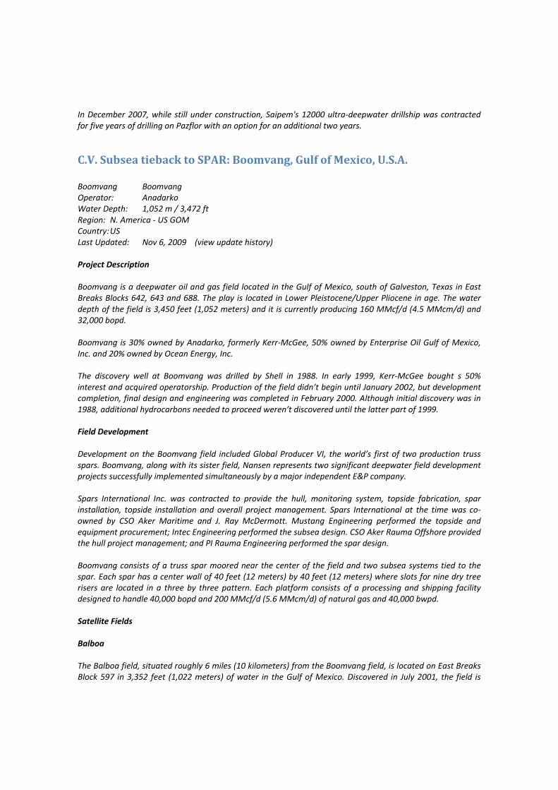
In December 2007, while still under construction, Saipem's 12000 ultra‐deepwater drillship was contracted for five years of drilling on Pazflor with an option for an additional two years.
C.V. Subsea tieback to SPAR: Boomvang, Gulf of Mexico, U.S.A. Boomvang Boomvang Operator: Anadarko Water Depth: 1,052 m / 3,472 ft Region: N. America ‐ US GOM Country: US Last Updated: Nov 6, 2009 (view update history) Project Description Boomvang is a deepwater oil and gas field located in the Gulf of Mexico, south of Galveston, Texas in East Breaks Blocks 642, 643 and 688. The play is located in Lower Pleistocene/Upper Pliocene in age. The water depth of the field is 3,450 feet (1,052 meters) and it is currently producing 160 MMcf/d (4.5 MMcm/d) and 32,000 bopd. Boomvang is 30% owned by Anadarko, formerly Kerr‐McGee, 50% owned by Enterprise Oil Gulf of Mexico, Inc. and 20% owned by Ocean Energy, Inc. The discovery well at Boomvang was drilled by Shell in 1988. In early 1999, Kerr‐McGee bought s 50% interest and acquired operatorship. Production of the field didn’t begin until January 2002, but development completion, final design and engineering was completed in February 2000. Although initial discovery was in 1988, additional hydrocarbons needed to proceed weren’t discovered until the latter part of 1999. Field Development Development on the Boomvang field included Global Producer VI, the world’s first of two production truss spars. Boomvang, along with its sister field, Nansen represents two significant deepwater field development projects successfully implemented simultaneously by a major independent E&P company. Spars International Inc. was contracted to provide the hull, monitoring system, topside fabrication, spar installation, topside installation and overall project management. Spars International at the time was co‐owned by CSO Aker Maritime and J. Ray McDermott. Mustang Engineering performed the topside and equipment procurement; Intec Engineering performed the subsea design. CSO Aker Rauma Offshore provided the hull project management; and PI Rauma Engineering performed the spar design. Boomvang consists of a truss spar moored near the center of the field and two subsea systems tied to the spar. Each spar has a center wall of 40 feet (12 meters) by 40 feet (12 meters) where slots for nine dry tree risers are located in a three by three pattern. Each platform consists of a processing and shipping facility designed to handle 40,000 bopd and 200 MMcf/d (5.6 MMcm/d) of natural gas and 40,000 bwpd. Satellite Fields Balboa The Balboa field, situated roughly 6 miles (10 kilometers) from the Boomvang field, is located on East Breaks Block 597 in 3,352 feet (1,022 meters) of water in the Gulf of Mexico. Discovered in July 2001, the field is
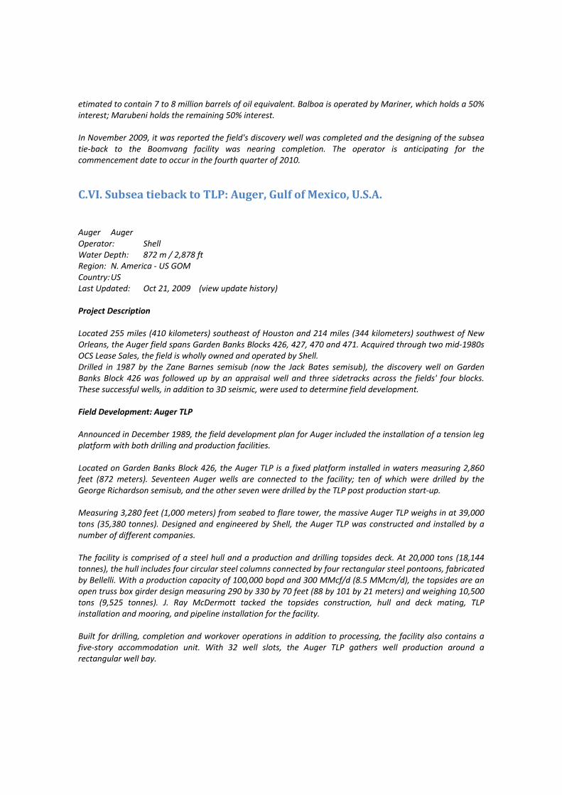
etimated to contain 7 to 8 million barrels of oil equivalent. Balboa is operated by Mariner, which holds a 50% interest; Marubeni holds the remaining 50% interest. In November 2009, it was reported the field's discovery well was completed and the designing of the subsea tie‐back to the Boomvang facility was nearing completion. The operator is anticipating for the commencement date to occur in the fourth quarter of 2010.
C.VI. Subsea tieback to TLP: Auger, Gulf of Mexico, U.S.A.
Auger Auger Operator: Shell Water Depth: 872 m / 2,878 ft Region: N. America ‐ US GOM Country: US Last Updated: Oct 21, 2009 (view update history) Project Description Located 255 miles (410 kilometers) southeast of Houston and 214 miles (344 kilometers) southwest of New Orleans, the Auger field spans Garden Banks Blocks 426, 427, 470 and 471. Acquired through two mid‐1980s OCS Lease Sales, the field is wholly owned and operated by Shell. Drilled in 1987 by the Zane Barnes semisub (now the Jack Bates semisub), the discovery well on Garden Banks Block 426 was followed up by an appraisal well and three sidetracks across the fields' four blocks. These successful wells, in addition to 3D seismic, were used to determine field development. Field Development: Auger TLP Announced in December 1989, the field development plan for Auger included the installation of a tension leg platform with both drilling and production facilities. Located on Garden Banks Block 426, the Auger TLP is a fixed platform installed in waters measuring 2,860 feet (872 meters). Seventeen Auger wells are connected to the facility; ten of which were drilled by the George Richardson semisub, and the other seven were drilled by the TLP post production start‐up. Measuring 3,280 feet (1,000 meters) from seabed to flare tower, the massive Auger TLP weighs in at 39,000 tons (35,380 tonnes). Designed and engineered by Shell, the Auger TLP was constructed and installed by a number of different companies. The facility is comprised of a steel hull and a production and drilling topsides deck. At 20,000 tons (18,144 tonnes), the hull includes four circular steel columns connected by four rectangular steel pontoons, fabricated by Bellelli. With a production capacity of 100,000 bopd and 300 MMcf/d (8.5 MMcm/d), the topsides are an open truss box girder design measuring 290 by 330 by 70 feet (88 by 101 by 21 meters) and weighing 10,500 tons (9,525 tonnes). J. Ray McDermott tacked the topsides construction, hull and deck mating, TLP installation and mooring, and pipeline installation for the facility. Built for drilling, completion and workover operations in addition to processing, the facility also contains a five‐story accommodation unit. With 32 well slots, the Auger TLP gathers well production around a rectangular well bay.
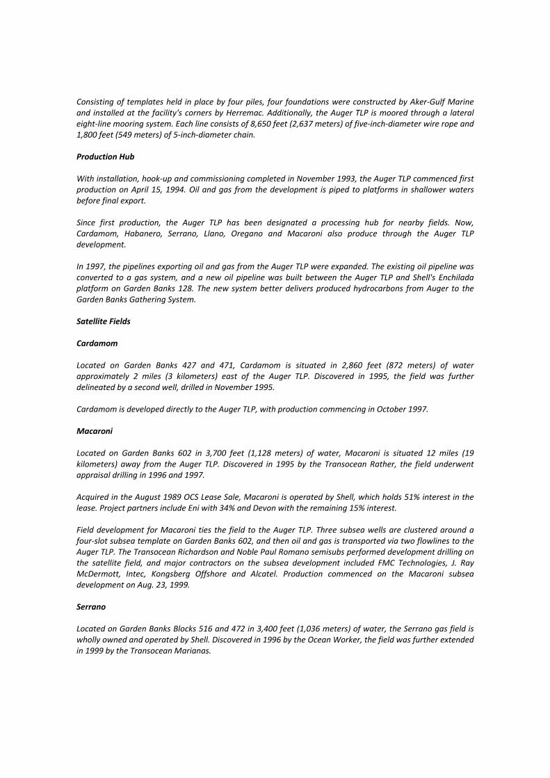
Consisting of templates held in place by four piles, four foundations were constructed by Aker‐Gulf Marine and installed at the facility's corners by Herremac. Additionally, the Auger TLP is moored through a lateral eight‐line mooring system. Each line consists of 8,650 feet (2,637 meters) of five‐inch‐diameter wire rope and 1,800 feet (549 meters) of 5‐inch‐diameter chain. Production Hub With installation, hook‐up and commissioning completed in November 1993, the Auger TLP commenced first production on April 15, 1994. Oil and gas from the development is piped to platforms in shallower waters before final export. Since first production, the Auger TLP has been designated a processing hub for nearby fields. Now, Cardamom, Habanero, Serrano, Llano, Oregano and Macaroni also produce through the Auger TLP development. In 1997, the pipelines exporting oil and gas from the Auger TLP were expanded. The existing oil pipeline was converted to a gas system, and a new oil pipeline was built between the Auger TLP and Shell's Enchilada platform on Garden Banks 128. The new system better delivers produced hydrocarbons from Auger to the Garden Banks Gathering System. Satellite Fields Cardamom Located on Garden Banks 427 and 471, Cardamom is situated in 2,860 feet (872 meters) of water approximately 2 miles (3 kilometers) east of the Auger TLP. Discovered in 1995, the field was further delineated by a second well, drilled in November 1995. Cardamom is developed directly to the Auger TLP, with production commencing in October 1997. Macaroni Located on Garden Banks 602 in 3,700 feet (1,128 meters) of water, Macaroni is situated 12 miles (19 kilometers) away from the Auger TLP. Discovered in 1995 by the Transocean Rather, the field underwent appraisal drilling in 1996 and 1997. Acquired in the August 1989 OCS Lease Sale, Macaroni is operated by Shell, which holds 51% interest in the lease. Project partners include Eni with 34% and Devon with the remaining 15% interest. Field development for Macaroni ties the field to the Auger TLP. Three subsea wells are clustered around a four‐slot subsea template on Garden Banks 602, and then oil and gas is transported via two flowlines to the Auger TLP. The Transocean Richardson and Noble Paul Romano semisubs performed development drilling on the satellite field, and major contractors on the subsea development included FMC Technologies, J. Ray McDermott, Intec, Kongsberg Offshore and Alcatel. Production commenced on the Macaroni subsea development on Aug. 23, 1999. Serrano Located on Garden Banks Blocks 516 and 472 in 3,400 feet (1,036 meters) of water, the Serrano gas field is wholly owned and operated by Shell. Discovered in 1996 by the Ocean Worker, the field was further extended in 1999 by the Transocean Marianas.
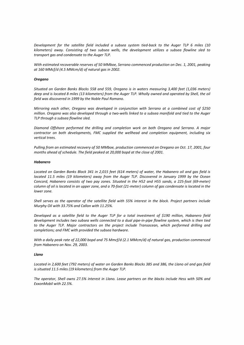
Development for the satellite field included a subsea system tied‐back to the Auger TLP 6 miles (10 kilometers) away. Consisting of two subsea wells, the development utilizes a subsea flowline sled to transport gas and condensate to the Auger TLP. With estimated recoverable reserves of 50 MMboe, Serrano commenced production on Dec. 1, 2001, peaking at 160 MMcf/d (4.5 MMcm/d) of natural gas in 2002. Oregano Situated on Garden Banks Blocks 558 and 559, Oregano is in waters measuring 3,400 feet (1,036 meters) deep and is located 8 miles (13 kilometers) from the Auger TLP. Wholly owned and operated by Shell, the oil field was discovered in 1999 by the Noble Paul Romano. Mirroring each other, Oregano was developed in conjunction with Serrano at a combined cost of $250 million. Oregano was also developed through a two‐wells linked to a subsea manifold and tied to the Auger TLP through a subsea flowline sled. Diamond Offshore performed the drilling and completion work on both Oregano and Serrano. A major contractor on both developments, FMC supplied the wellhead and completion equipment, including six vertical trees. Pulling from an estimated recovery of 50 MMboe, production commenced on Oregano on Oct. 17, 2001, four months ahead of schedule. The field peaked at 20,000 bopd at the close of 2001. Habanero Located on Garden Banks Block 341 in 2,015 feet (614 meters) of water, the Habanero oil and gas field is located 11.5 miles (19 kilometers) away from the Auger TLP. Discovered in January 1999 by the Ocean Concord, Habanero consists of two pay zones. Situated in the H52 and H55 sands, a 225‐foot (69‐meter) column of oil is located in an upper zone, and a 70‐foot (21‐meter) column of gas condensate is located in the lower zone. Shell serves as the operator of the satellite field with 55% interest in the block. Project partners include Murphy Oil with 33.75% and Callon with 11.25%. Developed as a satellite field to the Auger TLP for a total investment of $190 million, Habanero field development includes two subsea wells connected to a dual pipe‐in‐pipe flowline system, which is then tied to the Auger TLP. Major contractors on the project include Transocean, which performed drilling and completions; and FMC with provided the subsea hardware. With a daily peak rate of 22,000 bopd and 75 Mmcf/d (2.1 MMcm/d) of natural gas, production commenced from Habanero on Nov. 29, 2003. Llano Located in 2,600 feet (792 meters) of water on Garden Banks Blocks 385 and 386, the Llano oil and gas field is situated 11.5 miles (19 kilometers) from the Auger TLP. The operator, Shell owns 27.5% interest in Llano. Lease partners on the blocks include Hess with 50% and ExxonMobil with 22.5%.
Discovered in 1998 by the Transocean Voyager & Omega, the field was delineated by two sidetrack wells. Reserves are located in the Pliocene and Miocene formations at a thickness of 150 feet (46 meters) and 95 feet (29 meters), respectively. Developed as a subsea tie‐back to the Auger TLP, Llano field development includes two wells tied through a pipe‐in‐pipe looped flowline. FMC also served as a major contractor on this development. With a peak rate of 25,000 bopd and 75 MMcf/d (2.1 MMcm/d) of gas, production commenced from Llano on April 29, 2004. Ozona The Ozona oil and gas field is located in approxiamtely 3,280 feet (1,000 meters) of water on Garden Banks Block 515, about 175 miles southeast of Sabine, Texas. Marathon serves as the operator and holds a 68% interest; Marubeni holds the remaining 35% interest. At a development cost of $300 million, Ozona will consist of one well subsea tied‐back to the Auger platform, which is located six miles from the field. Ozona is expected to commence production in 2011 and reach a peak production of 6,000 bopd and 13 MMcf/d.
C.VII. Dry tree SPAR: Mad Dog Field, Gulf of Mexico, U.S.A. Mad Dog Field, Gulf of Mexico, USA Name: Mad Dog Location: Gulf of Mexico Operator: BP Distance from shore: 190 miles south of New Orleans Water depth: 4,500ft Equity: BP 60.5%, BHPBilliton 23.9%, Unocal 15.6% Drilling unit range: 5,000ft to 7,000ft of water The Mad Dog field is located in Western Atwater Foldbelt, Gulf of Mexico, approx. 190 miles south of New Orleans. The nominal water depth is 4,500ft and the field runs along the Sigsbee Escarpment. The field is operated by BP 60.5% on behalf of BHPBilliton 23.9% and Unocal 15.6%. The drilling unit is located in 5,000ft to 7,000ft of water in Green Canyon blocks 825, 826 and 782, about 150 miles southwest of Venice, Louisiana. The gross estimated reserves are in the range of 200 to 450 million barrels of oil equivalent. The development has cost $1.54 billion to bring onstream. The discovery well, in water depths of approx. 6,600ft, was spudded in May 1998 in Green Canyon 826 and was drilled to a measured depth of 22,410ft. The discovery was followed by a 1999 well drilled to a total depth of 22,410ft and a further successful appraisal well in February 2000. The project was sanctioned in 2001. Mad dog's pre‐drilled wells were drilled by the Ocean Confidence. The Mississippi fan fold belt is characterised by basinward‐verging anticlines and associated thrust faults. Mad Dog is one of a number of discoveries occurring in the western portion of the fold belt, where shallow salt tongues have flown over some of the folds, making seismic imaging difficult.
Development The field is being developed by 12 wells produced with a single‐piece truss spar permanently moored in 4,500ft water depths in Green Canyon Block 782, 306km south of New Orleans. The fabrication of the spar hull commenced in Finland in July 2002, and the topsides in Morgan City, Louisiana, one month later. Topsides The deck measures 220ft by 163ft by 50ft (67m x 50m x 15m) and was designed around the heaviest hook load available (around 8,000t). The host facility includes production facilities with 16 slots in a 4 x 4 pattern (13 production slots, a drilling riser slot and two service slots), and quarters for 126 personnel, although the temporary quarters can accommodate an additional 60 persons. The spar also has a BP‐owned drilling rig with an operating weight of 5,500t. HULL The 20,800t hull measures 128ft in diameter and is 555ft long. The facility is designed to process approximately 100,000 barrels of oil and 60mscf of gas per day. The spar has a maximum operating payload capacity of around 18,500t excluding hull storage. The topside and integrated decks total 10,500t The trus spar took three weeks to travel from Finland to Passagoula, Mississippi, on the Mighty Servant 1, where it was floated off and pre‐assembly preparations were completed. The Thialf was then used to lift the topsides into place. Mooring The spar is moored by an 11‐line taut mooring configuration. There are three mooring line groups ‐ two with four lines and one with three. The polyester mooring lines are attached to suction piles, resulting in a saving of around 1,000t of buoyancy over rope and chain systems. It is the first such use of synthetic moorings approved by the US Coast Guard or MMS. Oil from Mad Dog will be transported via the Caesar pipeline to Ship Shoal 332B, where it will interconnect with the Cameron Highway Oil Pipeline System (CHOPS). Mad Dog gas will be exported via the Cleopatra pipeline to Ship Shoal 332A, where it will interconnect with the Manta Ray Gathering System, and from there to the Nautilus Gas Transportation System into Louisiana. Both Caesar and Cleopatra pipelines are part of the BP‐operated Mardi Gras Transportation System.
C.VIII. Dry tree TLP: Matterhorn Field, Gulf of Mexico, U.S.A. Matterhorn Field, Gulf of Mexico, USA Operator: TotalFinaElf E&P USA Location: Mississippi Canyon Block 243, 170km southeast of New Orleans Water: 850m of water Production rate: 40,000 barrels of oil equivalent per day Production system: Mini tension leg platform Hull fabrication: Keppel Fels Main column diameter: 84ft
The Matterhorn field is located in Mississippi Canyon Block 243 in the deepwater Gulf of Mexico, approx. 170km southeast of New Orleans. It lies in 850m of water. The field came onstream in November 2003 and has a production capacity of 33,000 barrels of oil equivalent per day. "The field came onstream in November 2003 and has a production capacity of 33,000 barrels of oil equivalent per day." The Matterhrorn field is wholly owned and operated by TotalFinaElf E&P USA. After examining a number of development options, the designers settled on the use of a mini tension leg platform. The company opted for an Atlantia SeaStar design of the type previously installed on such deepwater projects as Chevron's Typhoon and British‐Borneo's (Agip) Morpeth and Allegheny fields. Because of the field however, a larger version than the existing designs was deemed necessary. The Matterhorn platform, at 4,500t, stands as the biggest of its type ‐ double the size of the previous units and the first unit of this design to incorporate supporting vertical access production flowlines running through the central moonpool and controlled by surface (dry) trees. The contract for the hull was won by Keppel Fels in Singapore, making Matterhorn also the first one built outside of the Gulf of Mexico. MATTERHORN SEASTAR HULL The fabrication of the Matterhorn SeaStar hull structure began on 28 January 2002 and was completed by the end of the year. The construction is based on a relatively large central main column with a diameter of 84ft. It has a design draft of 104ft. At the base of the column are three pontoons which project out to give the structure an effective radius of 179ft. At the point where they are attached to the main column the pontoon heights are 42 ft, however these taper down to just 27ft at the tip. "In early 2003, the structure was sailed out of Keppel Fels yard across to Pascaguola, Mississippi." This hull structure is designed to support a payload 16,850kips (thousand pounds). The hull itself will weigh approximately 12,280kips, of which the primary hull structure will account for 10,420kips. Altogether, the platform has a displacement of 52,800kips. In early 2003, the structure was sailed out of Keppel Fels yard across to Pascaguola, Mississippi, to await mating with the topsides. MATTERHORN TOPSIDES The Matterhorn topsides design is distributed over three decks. This deck arrangement was constructed at the Gulf Marine Fabricators in Ingleside, Texas. Paragon Engineering was responsible for the design of the topside facilities, employing the 3D PDMS (Plant Design Management System). The company expended over 60,000 man‐hours on the design. The deck free board is designated at 69ft and the decks have an area of 140ft². The operating weight of the decks and facilities is 13,350kips. In order to process the Matterhorn hydrocarbons the platform design has process capacities of 35,000b/d of oil, 55 million scf/d of gas, 20,000b/d of water treated and 30,000b/d of water injected. The wellbay design is centred on nine well slots although production currently flows through risers in only seven of them. Located at the top of the platform is a SuperSundowner XVI1,000hp drilling rig. Total also has one subsea injector well on the seafloor, leaving capacity for future tiebacks.
The design includes quarters for 22 men. The Matterhorn TLP is connected to the seabed by six 32in neutrally buoyant steel tubular tendons. These were fabricated by Kiewit Offshore Service, also in Ingleside. Each tendon is secured by means of an independent, 96in‐diameter, 415ft pile at the seabed, fabricated by Gulf Marine Fabricators. At 400t, the piles are among the heaviest ever installed. The offshore installation was carried out by Heerema's Balder crane vessel.
References:
1. Offshore Technology, “Mad Dog Field, Gulf of Mexico, USA” Industry Projects. Available in Internet at http://www.offshore‐technology.com/projects/mad_dog last visited May 1st, 2010.
2. Offshore Technology, “Matterhorn Field, Gulf of Mexico, USA” Industry Projects. Available in Internet at http://www.offshore‐technology.com/projects/matterhorn last visited May 1st, 2010.
3. Subsea IQ, “Auger” Offshore Field Development Projects. Available in Internet at http://www.subseaiq.com/data/Project.aspx?project_id=139 last visited May 1st, 2010.
4. Subsea IQ, “Boomvang” Offshore Field Development Projects. Available in Internet at http://www.subseaiq.com/data/Project.aspx?project_id=118 last visited May 1st, 2010.
5. Subsea IQ, “Canyon Express” Offshore Field Development Projects. Available in Internet at http://www.subseaiq.com/data/Project.aspx?project_id=115 last visited May 1st, 2010.
6. Subsea IQ, “Ormen Lange” Offshore Field Development Projects. Available in Internet at http://www.subseaiq.com/data/Project.aspx?project_id=222 last visited May 1st, 2010.
7. Subsea IQ, “Pazflor” Offshore Field Development Projects. Available in Internet at http://www.subseaiq.com/data/Project.aspx?project_id=326 last visited May 1st, 2010.
8. Subsea IQ, “Tunder Horse” Offshore Field Development Projects. Available in Internet at http://www.subseaiq.com/data/Project.aspx?project_id=129 last visited May 1st, 2010.
Annex D: Marine Operations The Marine operations may have quite different purposes. However, there are commonly referenced documents that are followed by the most of the marine contractors, one of those is the “DNV Rules for Planning and Execution of Marine Operations” (DNV, 2008). The Rules for Planning and Execution of Marine Operations lay down technical and procedural requirements related to proper planning and execution of marine operations such as:
• Load Transfer Operations (issued 1996). • Towing (issued 1996). • Special Sea Transports (issued 1996). • Offshore Installation (issued 1996). • Lifting (issued 1996). • Sub Sea Operations (issued 1996). • Transit and Positioning of Mobile Offshore Units (issued 2000).
Noble Denton is also a company that proposes guidelines commonly cited on marine operations planning and execution. Some of those guidelines are listed below.
• 0009/ND operations. • 0013/ND Rev 4 ‐ 19 Jan 2009 Guidelines for loadouts. • 0015/ND Rev 1 ‐ 16 Dec 2008 Concrete offshore gravity structures/constr., tow. &
install. • 0016/ND Rev 4 ‐ 16 Dec 2008 Seabed and sub‐seabed data for approvals of mobile
offshore units/MOU. • 0021/ND Rev 7 ‐ 17 Nov 2008 Guidelines for the approval of towing vessels. • 0027/ND Rev 8 ‐ 23 June 2009 Guidelines for marine lifting operations. • 0028/ND Rev 3 ‐ 19 Jan 2009 Guidelines for the transportation and installation of steel
jackets. • 0030/NDI Rev 3 ‐ 15 April 2009 Guidelines for marine transportations.
One of the most important factors for marine operations are the weather conditions that prevail during operations, each operation has its limits in terms of wave and tidal height and speed of currents and winds for its various operating scenarios, whether they are survival, transfer, installation and normal operation. See the previously cited guidelines for more information and the document "Uncertainties in weatherforecasting, a risk to offshore operations (Gudmestad, 1999), for more information. On this matter, Gudmestad (Gudmestad, 2001) proposed risk assessment tools for use in projects and offshore marine operations. His proposal emphasizes the vulnerability to climatic conditions, such as in deepwater projects during the installation period. He said, it is particularly important consider that vulnerability since some project management philosophies are more focused on implementing cost effective operations. This leads to a high probability that complex operations are carried out in the “winter” season here the ranges with appropriate climate grow shorter and the changes in weather conditions are more frequent and more rapid than the "summer season".
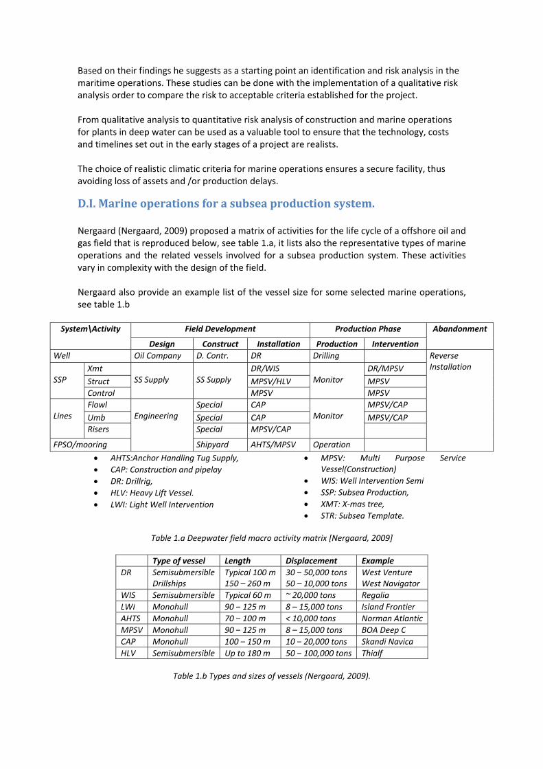
Based on their findings he suggests as a starting point an identification and risk analysis in the maritime operations. These studies can be done with the implementation of a qualitative risk analysis order to compare the risk to acceptable criteria established for the project. From qualitative analysis to quantitative risk analysis of construction and marine operations for plants in deep water can be used as a valuable tool to ensure that the technology, costs and timelines set out in the early stages of a project are realists. The choice of realistic climatic criteria for marine operations ensures a secure facility, thus avoiding loss of assets and /or production delays.
D.I. Marine operations for a subsea production system. Nergaard (Nergaard, 2009) proposed a matrix of activities for the life cycle of a offshore oil and gas field that is reproduced below, see table 1.a, it lists also the representative types of marine operations and the related vessels involved for a subsea production system. These activities vary in complexity with the design of the field. Nergaard also provide an example list of the vessel size for some selected marine operations, see table 1.b
System\Activity Field Development Production Phase Abandonment
Design Construct Installation Production Intervention Well Oil Company D. Contr. DR Drilling Reverse
Installation
SSP
Xmt SS Supply
SS Supply
DR/WISMonitor
DR/MPSV Struct MPSV/HLV MPSV Control MPSV MPSV
Lines
Flowl Engineering
Special CAPMonitor
MPSV/CAP Umb Special CAP MPSV/CAP Risers Special MPSV/CAP
FPSO/mooring Shipyard AHTS/MPSV Operation
• AHTS:Anchor Handling Tug Supply, • CAP: Construction and pipelay • DR: Drillrig, • HLV: Heavy Lift Vessel. • LWI: Light Well Intervention
• MPSV: Multi Purpose Service Vessel(Construction)
• WIS: Well Intervention Semi • SSP: Subsea Production, • XMT: X‐mas tree, • STR: Subsea Template.
Table 1.a Deepwater field macro activity matrix [Nergaard, 2009]
Type of vessel Length Displacement Example DR Semisubmersible
Drillships Typical 100 m150 – 260 m
30 – 50,000 tons50 – 10,000 tons
West Venture West Navigator
WIS Semisubmersible Typical 60 m ~ 20,000 tons Regalia LWI Monohull 90 – 125 m 8 – 15,000 tons Island Frontier AHTS Monohull 70 – 100 m < 10,000 tons Norman Atlantic MPSV Monohull 90 – 125 m 8 – 15,000 tons BOA Deep C CAP Monohull 100 – 150 m 10 – 20,000 tons Skandi Navica HLV Semisubmersible Up to 180 m 50 – 100,000 tons Thialf
Table 1.b Types and sizes of vessels (Nergaard, 2009).
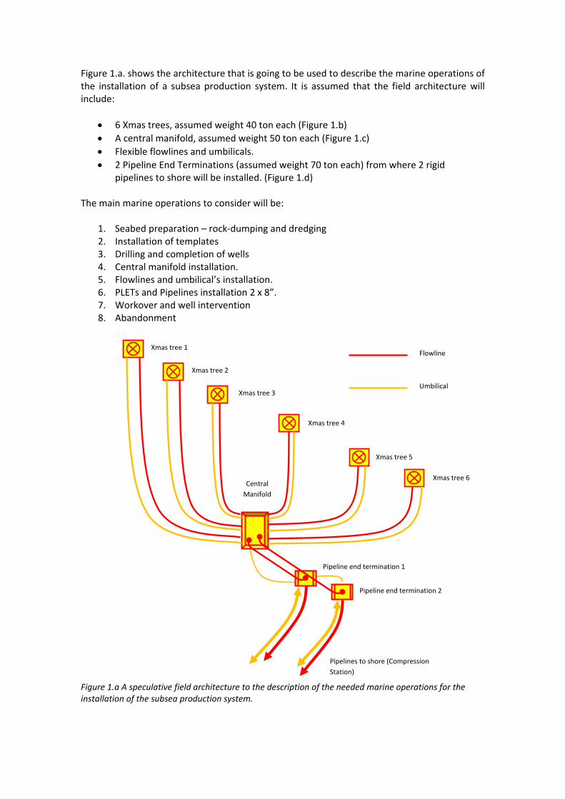
Figure 1.a. shows the architecture that is going to be used to describe the marine operations of the installation of a subsea production system. It is assumed that the field architecture will include:
• 6 Xmas trees, assumed weight 40 ton each (Figure 1.b) • A central manifold, assumed weight 50 ton each (Figure 1.c) • Flexible flowlines and umbilicals. • 2 Pipeline End Terminations (assumed weight 70 ton each) from where 2 rigid
pipelines to shore will be installed. (Figure 1.d) The main marine operations to consider will be:
1. Seabed preparation – rock‐dumping and dredging 2. Installation of templates 3. Drilling and completion of wells 4. Central manifold installation. 5. Flowlines and umbilical’s installation. 6. PLETs and Pipelines installation 2 x 8”. 7. Workover and well intervention 8. Abandonment
Figure 1.a A speculative field architecture to the description of the needed marine operations for the installation of the subsea production system.
Xmas tree 1
Xmas tree 3
Xmas tree 2
Xmas tree 4
Xmas tree 5
Xmas tree 6
Flowline
Umbilical
Central Manifold
Pipeline end termination 1
Pipeline end termination 2
Pipelines to shore (Compression Station)
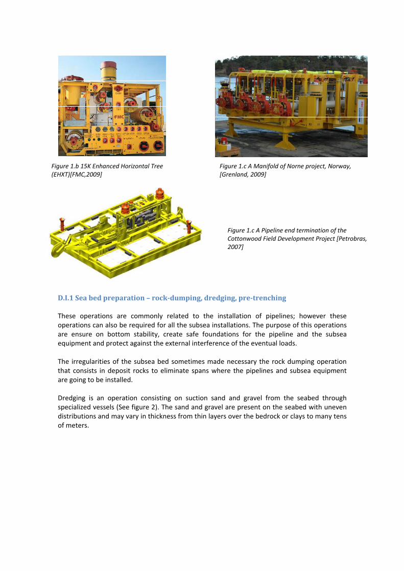
D.I.1 Sea bed preparation – rockdumping, dredging, pretrenching These operations are commonly related to the installation of pipelines; however these operations can also be required for all the subsea installations. The purpose of this operations are ensure on bottom stability, create safe foundations for the pipeline and the subsea equipment and protect against the external interference of the eventual loads.
The irregularities of the subsea bed sometimes made necessary the rock dumping operation that consists in deposit rocks to eliminate spans where the pipelines and subsea equipment are going to be installed.
Dredging is an operation consisting on suction sand and gravel from the seabed through specialized vessels (See figure 2). The sand and gravel are present on the seabed with uneven distributions and may vary in thickness from thin layers over the bedrock or clays to many tens of meters.
Figure 1.b 15K Enhanced Horizontal Tree (EHXT)[FMC,2009]
Figure 1.c A Manifold of Norne project, Norway, [Grenland, 2009]
Figure 1.c A Pipeline end termination of the Cottonwood Field Development Project [Petrobras, 2007]
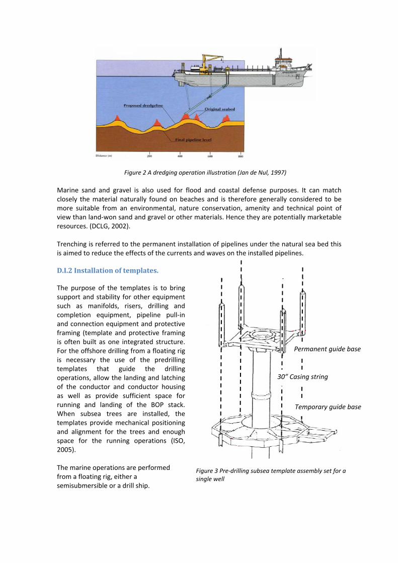
Figure 3 Pre‐drilling subsea template assembly set for a single well
Temporary guide base
Permanent guide base
30” Casing string
Figure 2 A dredging operation illustration (Jan de Nul, 1997)
Marine sand and gravel is also used for flood and coastal defense purposes. It can match closely the material naturally found on beaches and is therefore generally considered to be more suitable from an environmental, nature conservation, amenity and technical point of view than land‐won sand and gravel or other materials. Hence they are potentially marketable resources. (DCLG, 2002). Trenching is referred to the permanent installation of pipelines under the natural sea bed this is aimed to reduce the effects of the currents and waves on the installed pipelines. D.I.2 Installation of templates. The purpose of the templates is to bring support and stability for other equipment such as manifolds, risers, drilling and completion equipment, pipeline pull‐in and connection equipment and protective framing (template and protective framing is often built as one integrated structure. For the offshore drilling from a floating rig is necessary the use of the predrilling templates that guide the drilling operations, allow the landing and latching of the conductor and conductor housing as well as provide sufficient space for running and landing of the BOP stack. When subsea trees are installed, the templates provide mechanical positioning and alignment for the trees and enough space for the running operations (ISO, 2005). The marine operations are performed from a floating rig, either a semisubmersible or a drill ship.
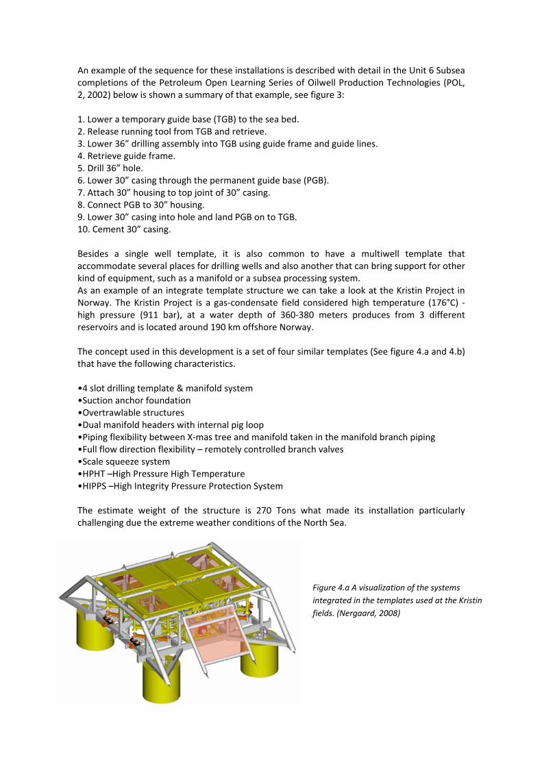
An example of the sequence for these installations is described with detail in the Unit 6 Subsea completions of the Petroleum Open Learning Series of Oilwell Production Technologies (POL, 2, 2002) below is shown a summary of that example, see figure 3: 1. Lower a temporary guide base (TGB) to the sea bed. 2. Release running tool from TGB and retrieve. 3. Lower 36” drilling assembly into TGB using guide frame and guide lines. 4. Retrieve guide frame. 5. Drill 36” hole. 6. Lower 30” casing through the permanent guide base (PGB). 7. Attach 30” housing to top joint of 30” casing. 8. Connect PGB to 30” housing. 9. Lower 30” casing into hole and land PGB on to TGB. 10. Cement 30” casing. Besides a single well template, it is also common to have a multiwell template that accommodate several places for drilling wells and also another that can bring support for other kind of equipment, such as a manifold or a subsea processing system. As an example of an integrate template structure we can take a look at the Kristin Project in Norway. The Kristin Project is a gas‐condensate field considered high temperature (176°C) ‐ high pressure (911 bar), at a water depth of 360‐380 meters produces from 3 different reservoirs and is located around 190 km offshore Norway. The concept used in this development is a set of four similar templates (See figure 4.a and 4.b) that have the following characteristics. •4 slot drilling template & manifold system •Suction anchor foundation •Overtrawlable structures •Dual manifold headers with internal pig loop •Piping flexibility between X‐mas tree and manifold taken in the manifold branch piping •Full flow direction flexibility – remotely controlled branch valves •Scale squeeze system •HPHT –High Pressure High Temperature •HIPPS –High Integrity Pressure Protection System The estimate weight of the structure is 270 Tons what made its installation particularly challenging due the extreme weather conditions of the North Sea.
Figure 4.a A visualization of the systems integrated in the templates used at the Kristin fields. (Nergaard, 2008)
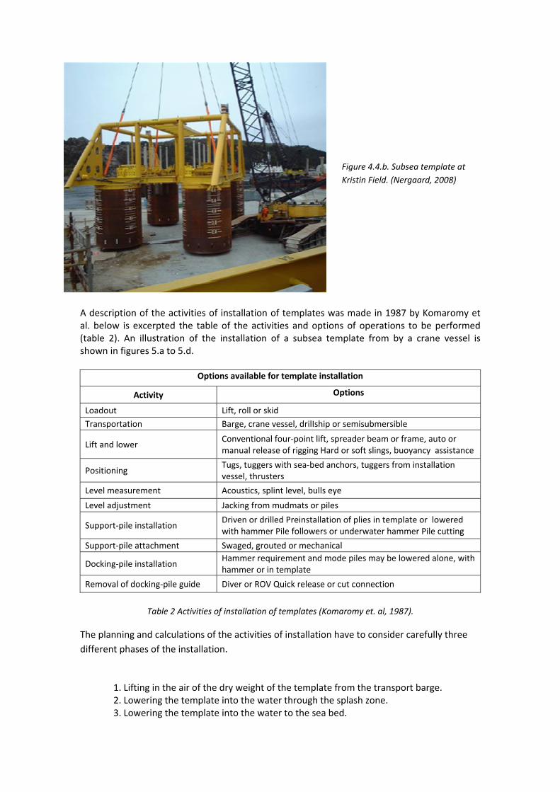
A description of the activities of installation of templates was made in 1987 by Komaromy et al. below is excerpted the table of the activities and options of operations to be performed (table 2). An illustration of the installation of a subsea template from by a crane vessel is shown in figures 5.a to 5.d.
Options available for template installation
Activity Options
Loadout Lift, roll or skid Transportation Barge, crane vessel, drilIship or semisubmersible
Lift and lower Conventional four‐point lift, spreader beam or frame, auto or manual release of rigging Hard or soft slings, buoyancy assistance
Positioning Tugs, tuggers with sea‐bed anchors, tuggers from installation vessel, thrusters
Level measurement Acoustics, splint level, bulls eye
Level adjustment Jacking from mudmats or piles
Support‐pile installation Driven or drilled Preinstallation of plies in template or lowered with hammer Pile followers or underwater hammer Pile cutting
Support‐pile attachment Swaged, grouted or mechanical
Docking‐pile installation Hammer requirement and mode piles may be lowered alone, with hammer or in template
Removal of docking‐pile guide Diver or ROV Quick release or cut connection
Table 2 Activities of installation of templates (Komaromy et. al, 1987).
The planning and calculations of the activities of installation have to consider carefully three different phases of the installation.
1. Lifting in the air of the dry weight of the template from the transport barge. 2. Lowering the template into the water through the splash zone. 3. Lowering the template into the water to the sea bed.
Figure 4.4.b. Subsea template at Kristin Field. (Nergaard, 2008)
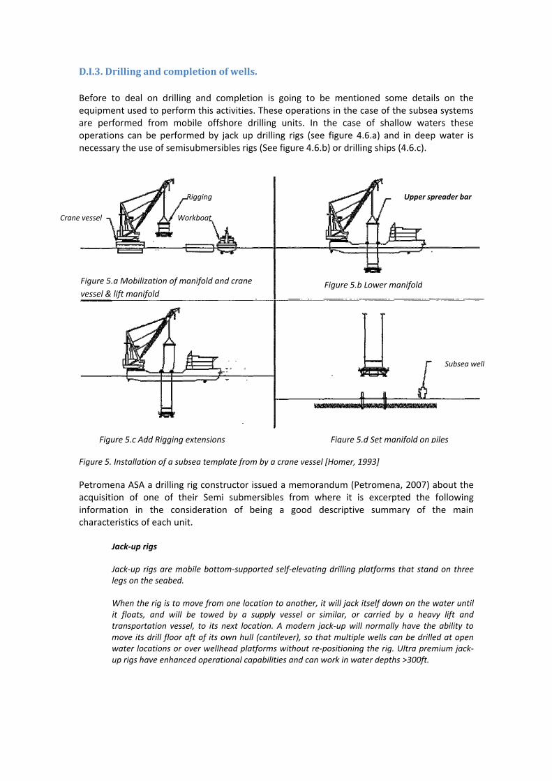
D.I.3. Drilling and completion of wells. Before to deal on drilling and completion is going to be mentioned some details on the equipment used to perform this activities. These operations in the case of the subsea systems are performed from mobile offshore drilling units. In the case of shallow waters these operations can be performed by jack up drilling rigs (see figure 4.6.a) and in deep water is necessary the use of semisubmersibles rigs (See figure 4.6.b) or drilling ships (4.6.c).
Figure 5. Installation of a subsea template from by a crane vessel [Homer, 1993]
Petromena ASA a drilling rig constructor issued a memorandum (Petromena, 2007) about the acquisition of one of their Semi submersibles from where it is excerpted the following information in the consideration of being a good descriptive summary of the main characteristics of each unit.
Jack‐up rigs Jack‐up rigs are mobile bottom‐supported self‐elevating drilling platforms that stand on three legs on the seabed. When the rig is to move from one location to another, it will jack itself down on the water until it floats, and will be towed by a supply vessel or similar, or carried by a heavy lift and transportation vessel, to its next location. A modern jack‐up will normally have the ability to move its drill floor aft of its own hull (cantilever), so that multiple wells can be drilled at open water locations or over wellhead platforms without re‐positioning the rig. Ultra premium jack‐up rigs have enhanced operational capabilities and can work in water depths >300ft.
Figure 5.a Mobilization of manifold and crane vessel & lift manifold
Figure 5.b Lower manifold
Figure 5.c Add Rigging extensions Figure 5.d Set manifold on piles
Upper spreader bar Rigging
Crane vessel Workboat
Subsea well
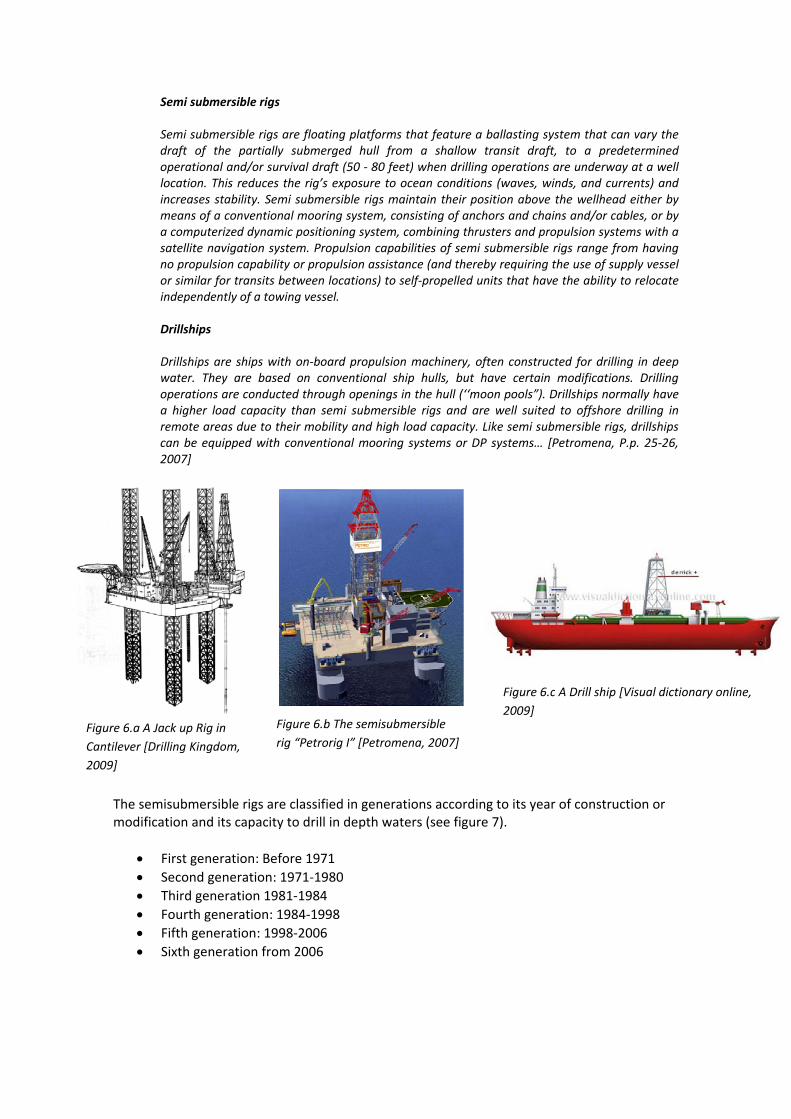
Semi submersible rigs Semi submersible rigs are floating platforms that feature a ballasting system that can vary the draft of the partially submerged hull from a shallow transit draft, to a predetermined operational and/or survival draft (50 ‐ 80 feet) when drilling operations are underway at a well location. This reduces the rig’s exposure to ocean conditions (waves, winds, and currents) and increases stability. Semi submersible rigs maintain their position above the wellhead either by means of a conventional mooring system, consisting of anchors and chains and/or cables, or by a computerized dynamic positioning system, combining thrusters and propulsion systems with a satellite navigation system. Propulsion capabilities of semi submersible rigs range from having no propulsion capability or propulsion assistance (and thereby requiring the use of supply vessel or similar for transits between locations) to self‐propelled units that have the ability to relocate independently of a towing vessel. Drillships Drillships are ships with on‐board propulsion machinery, often constructed for drilling in deep water. They are based on conventional ship hulls, but have certain modifications. Drilling operations are conducted through openings in the hull (‘‘moon pools”). Drillships normally have a higher load capacity than semi submersible rigs and are well suited to offshore drilling in remote areas due to their mobility and high load capacity. Like semi submersible rigs, drillships can be equipped with conventional mooring systems or DP systems… [Petromena, P.p. 25‐26, 2007]
The semisubmersible rigs are classified in generations according to its year of construction or modification and its capacity to drill in depth waters (see figure 7).
• First generation: Before 1971 • Second generation: 1971‐1980 • Third generation 1981‐1984 • Fourth generation: 1984‐1998 • Fifth generation: 1998‐2006 • Sixth generation from 2006
Figure 6.a A Jack up Rig in Cantilever [Drilling Kingdom, 2009]
Figure 6.c A Drill ship [Visual dictionary online, 2009]
Figure 6.b The semisubmersible rig “Petrorig I” [Petromena, 2007]
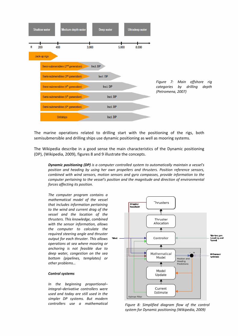
The marine operations related to drilling start with the positioning of the rigs, both semisubmersible and drilling ships use dynamic positioning as well as mooring systems. The Wikipedia describe in a good sense the main characteristics of the Dynamic positioning (DP), (Wikipedia, 2009), figures 8 and 9 illustrate the concepts.
Dynamic positioning (DP) is a computer controlled system to automatically maintain a vessel's position and heading by using her own propellers and thrusters. Position reference sensors, combined with wind sensors, motion sensors and gyro compasses, provide information to the computer pertaining to the vessel's position and the magnitude and direction of environmental forces affecting its position.
The computer program contains a mathematical model of the vessel that includes information pertaining to the wind and current drag of the vessel and the location of the thrusters. This knowledge, combined with the sensor information, allows the computer to calculate the required steering angle and thruster output for each thruster. This allows operations at sea where mooring or anchoring is not feasible due to deep water, congestion on the sea bottom (pipelines, templates) or other problems…
Control systems
In the beginning proportional–integral–derivative controllers were used and today are still used in the simpler DP systems. But modern controllers use a mathematical
Figure 7: Main offshore rig categories by drilling depth (Petromena, 2007)
Figure 8: Simplified diagram flow of the control system for Dynamic positioning (Wikipedia, 2009)
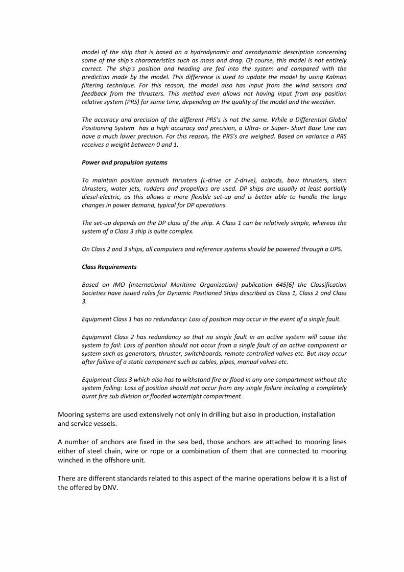
model of the ship that is based on a hydrodynamic and aerodynamic description concerning some of the ship's characteristics such as mass and drag. Of course, this model is not entirely correct. The ship's position and heading are fed into the system and compared with the prediction made by the model. This difference is used to update the model by using Kalman filtering technique. For this reason, the model also has input from the wind sensors and feedback from the thrusters. This method even allows not having input from any position relative system (PRS) for some time, depending on the quality of the model and the weather.
The accuracy and precision of the different PRS’s is not the same. While a Differential Global Positioning System has a high accuracy and precision, a Ultra‐ or Super‐ Short Base Line can have a much lower precision. For this reason, the PRS’s are weighed. Based on variance a PRS receives a weight between 0 and 1.
Power and propulsion systems
To maintain position azimuth thrusters (L‐drive or Z‐drive), azipods, bow thrusters, stern thrusters, water jets, rudders and propellors are used. DP ships are usually at least partially diesel‐electric, as this allows a more flexible set‐up and is better able to handle the large changes in power demand, typical for DP operations.
The set‐up depends on the DP class of the ship. A Class 1 can be relatively simple, whereas the system of a Class 3 ship is quite complex.
On Class 2 and 3 ships, all computers and reference systems should be powered through a UPS.
Class Requirements
Based on IMO (International Maritime Organization) publication 645[6] the Classification Societies have issued rules for Dynamic Positioned Ships described as Class 1, Class 2 and Class 3.
Equipment Class 1 has no redundancy: Loss of position may occur in the event of a single fault.
Equipment Class 2 has redundancy so that no single fault in an active system will cause the system to fail: Loss of position should not occur from a single fault of an active component or system such as generators, thruster, switchboards, remote controlled valves etc. But may occur after failure of a static component such as cables, pipes, manual valves etc.
Equipment Class 3 which also has to withstand fire or flood in any one compartment without the system failing: Loss of position should not occur from any single failure including a completely burnt fire sub division or flooded watertight compartment.
Mooring systems are used extensively not only in drilling but also in production, installation and service vessels. A number of anchors are fixed in the sea bed, those anchors are attached to mooring lines either of steel chain, wire or rope or a combination of them that are connected to mooring winched in the offshore unit. There are different standards related to this aspect of the marine operations below it is a list of the offered by DNV.
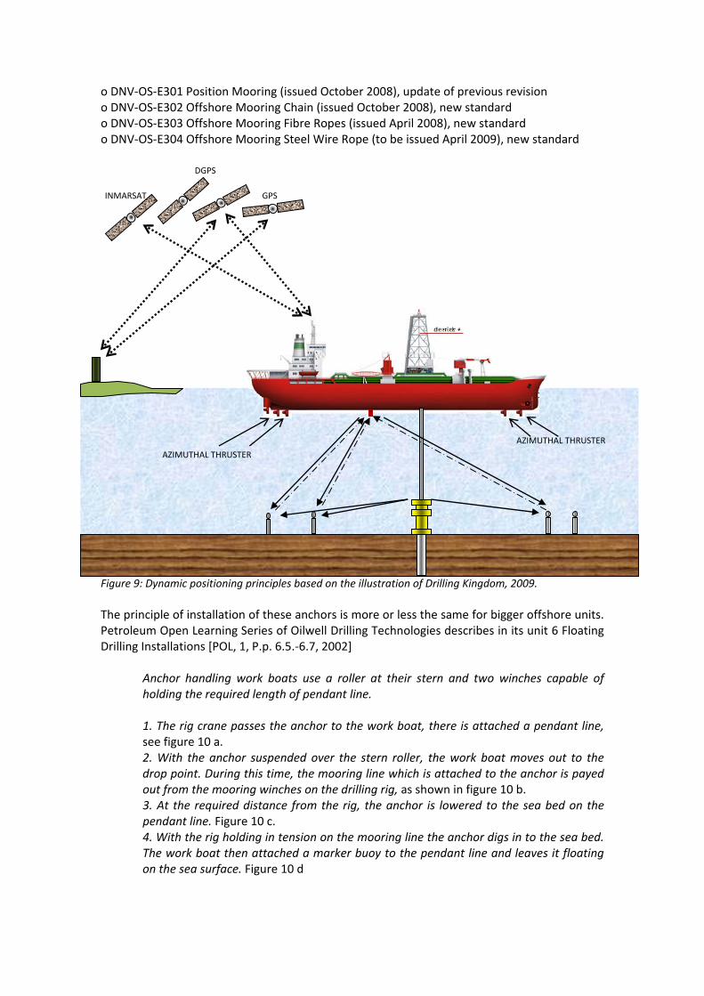
o DNV‐OS‐E301 Position Mooring (issued October 2008), update of previous revision o DNV‐OS‐E302 Offshore Mooring Chain (issued October 2008), new standard o DNV‐OS‐E303 Offshore Mooring Fibre Ropes (issued April 2008), new standard o DNV‐OS‐E304 Offshore Mooring Steel Wire Rope (to be issued April 2009), new standard Figure 9: Dynamic positioning principles based on the illustration of Drilling Kingdom, 2009. The principle of installation of these anchors is more or less the same for bigger offshore units. Petroleum Open Learning Series of Oilwell Drilling Technologies describes in its unit 6 Floating Drilling Installations [POL, 1, P.p. 6.5.‐6.7, 2002]
Anchor handling work boats use a roller at their stern and two winches capable of holding the required length of pendant line. 1. The rig crane passes the anchor to the work boat, there is attached a pendant line, see figure 10 a. 2. With the anchor suspended over the stern roller, the work boat moves out to the drop point. During this time, the mooring line which is attached to the anchor is payed out from the mooring winches on the drilling rig, as shown in figure 10 b. 3. At the required distance from the rig, the anchor is lowered to the sea bed on the pendant line. Figure 10 c. 4. With the rig holding in tension on the mooring line the anchor digs in to the sea bed. The work boat then attached a marker buoy to the pendant line and leaves it floating on the sea surface. Figure 10 d
DGPS
INMARSAT GPS
AZIMUTHAL THRUSTER
AZIMUTHAL THRUSTER
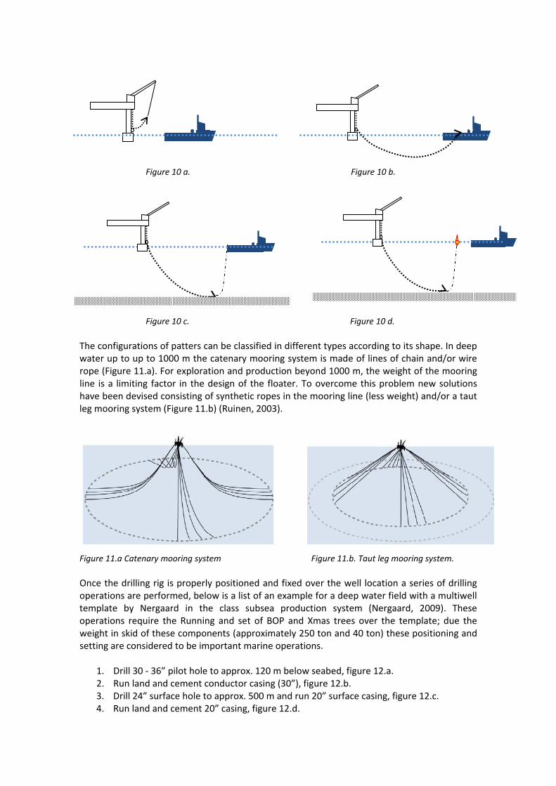
Figure 10 a. Figure 10 b.
Figure 10 c. Figure 10 d. The configurations of patters can be classified in different types according to its shape. In deep water up to up to 1000 m the catenary mooring system is made of lines of chain and/or wire rope (Figure 11.a). For exploration and production beyond 1000 m, the weight of the mooring line is a limiting factor in the design of the floater. To overcome this problem new solutions have been devised consisting of synthetic ropes in the mooring line (less weight) and/or a taut leg mooring system (Figure 11.b) (Ruinen, 2003). Figure 11.a Catenary mooring system Figure 11.b. Taut leg mooring system. Once the drilling rig is properly positioned and fixed over the well location a series of drilling operations are performed, below is a list of an example for a deep water field with a multiwell template by Nergaard in the class subsea production system (Nergaard, 2009). These operations require the Running and set of BOP and Xmas trees over the template; due the weight in skid of these components (approximately 250 ton and 40 ton) these positioning and setting are considered to be important marine operations.
1. Drill 30 ‐ 36” pilot hole to approx. 120 m below seabed, figure 12.a. 2. Run land and cement conductor casing (30”), figure 12.b. 3. Drill 24” surface hole to approx. 500 m and run 20” surface casing, figure 12.c. 4. Run land and cement 20” casing, figure 12.d.
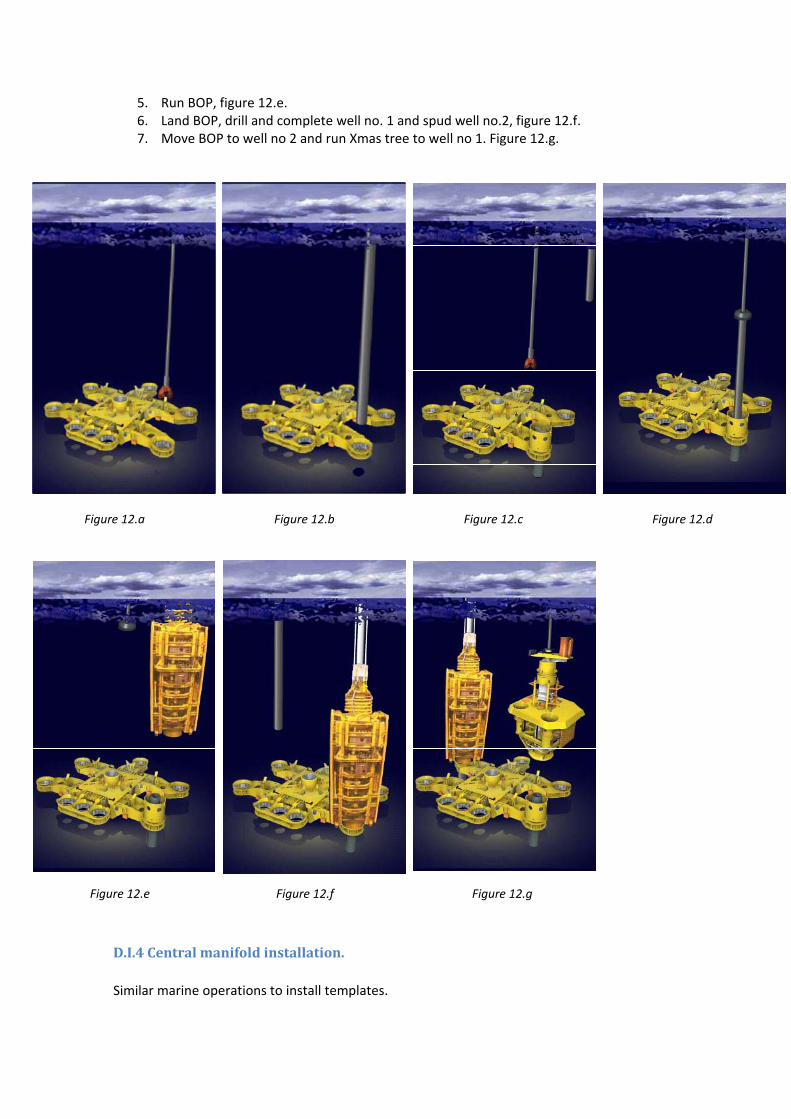
5. Run BOP, figure 12.e. 6. Land BOP, drill and complete well no. 1 and spud well no.2, figure 12.f. 7. Move BOP to well no 2 and run Xmas tree to well no 1. Figure 12.g.
D.I.4 Central manifold installation. Similar marine operations to install templates.
Figure 12.a Figure 12.b Figure 12.c Figure 12.d
Figure 12.e Figure 12.f Figure 12.g
D.I.5 Flowlines and umbilical’s installation. A good summary on how to install and connect flowlines and umbilicals is available in the appendix A, Sections A.9.2 and A.9.3 of the International Standard ISO 13628‐1 Design and operation of subsea production systems.
A.9.2 Flowline and umbilical configurations and installation techniques A.9.2.1 General Many factors need to be taken into account in the design of the flowlines and umbilicals for a subsea production system. The combination of through‐life design requirements, installation options and life‐cyclecosts will result in the selection of a preferred configuration and installation technique, the basic ones of which are outlined below. A.9.2.2 Individual flowlines Individual flowlines can be installed using S‐lay, J‐lay, reel (including pipe‐in‐pipe) and/or tow techniques as follows: ‐ S‐lay; The flowline is made up in a horizontal or near horizontal position on the lay vessel and lowered to the seafloor in an elongated “S” shape as the vessel moves forward. ‐ J‐lay; The flowline is made up in a vertical or near‐vertical position on the lay vessel and lowered to the seafloor in a near‐vertical orientation. This approach eliminates the overbend region of the S‐lay pipe catenary. ‐ Reel; The flowline is made up onshore and spooled onto a reel. The line is then transported to the desired location and unreeled onto the seafloor. The axis of the reel may be vertical or horizontal. ‐ tow. The flowline is made up onshore or in a mild offshore environment and then towed to its final location, where the buoyancy is adjusted to lower the line to the seafloor and provide adequate on‐bottom stability. There are several versions of the tow method, including the near‐surface tow, controlled‐depth tow, nearbottom tow and bottom tow. The tow methods differ primarily in the requirements for buoyancy control and in their sensitivity to environmental loadings during the towout. All of these techniques have limits with respect to the largest diameter lines that can be fabricated and installed. Reeling and towing also have some restrictions with respect to the length of line that can be fabricated and installed in a single run/unit. Whereas the host end of a reeled flowline can be pulled up a J‐or I‐tube, most of the other techniques rely on the use of spools/jumpers at the host end. In the case of a tieback to an FPS, the tail end of an individual rigid pipe or flexible pipe may be suspended from the FPS to form a riser, as described in A.10.3. The various connection options for the ends of individually installed flowlines are described in detail in A.9.9.
A.9.2.3 Bundles Small numbers of flowlines and/or umbilicals can be strapped together during reeling operations to form a strapped bundle on the seabed. While this configuration can have some advantages in terms of on‐bottom stability of the lines, etc., the benefits are somewhat limited as each line shall be at least partially designed on a stand‐alone basis...[ISO‐13628‐1, P.p. 131‐132, 2005]. A.9.3 Flowline and umbilical end connections A.9.3.1 General In order for a flowline or umbilical to fulfil its intended function, it is necessary to connect it to the associated subsea/surface facility equipment. A wide variety of techniques are available to complete this task, ranging from installation of flexible jumpers by divers at the subsea end of a flowline, through to pulling a multicore umbilical up through a J‐tube preinstalled on a production platform. For connection of flowlines and umbilicals to subsea/surface equipment, the basic steps involved in the process are the following: ‐ pull‐in of the two halves of the connector so that the faces are aligned and in close proximity (alternatively, the gap between the two halves of the connection may be spanned by an additional short length of sealine known as a jumper or spool); ‐ connection of the two halves of the connector; ‐ testing of the completed connection, to confirm that it has been successfully made up. ...[ISO‐13628‐1, P.p. 133‐134, 2005].
D.I.6 PLETs and Pipelines installation 2 x 8”. Pipelines are installed in at least 4 different methods, J‐Lay, S‐lay, Reel‐Lay and Normal‐lay (towed pipelines), of them the most suitable for the depth of the Lakach field would be a J‐lay with flexibility to use a S‐lay system also. A description of the advantages and disadvantages of the J lay given by Nogeira is reproduced in the table 3 (Nogeira, P.p. 931, 2005). A PLET (Pipeline End termination) is a structural‐transportation element in the subsea pipelines, as indicated in its name it is located at the end of the pipeline and is usually installed in the installation vessel and then lowered and positioned in the sea floor. Antani et. al. documented the installation of PLETS in the Neptune project in 2008, below it is a excerpt of their work that explain the procedure of installation of a PLET.
Advantages Disadvantages Best suited for ultra deep water pipeline installation.
Some vessels require the use of j lay collars to hold the pipe.
Suited for all the diameters. If shallower water pipeline installation is required in the same route, the J‐lay tower must be lowered to a less steep angle. Even then, depending on the water depth, it may not be feasible to J‐lay the shallow end with a particular vessel and a dual (J‐lay/S‐lay) installation may be required. Such as the case of the Canyon Express project.
Smallest bottom tension of all methods, which leads to the smallest route radius, and allows more flexibility for route layout. This may be important in congested areas. Can tipically handle in‐line appurtenances with relative ease, with respect to landing on the seafloor but within the constrains of the J‐lay tower. Table 3 Advantages and disadvantages of the J lay construction method for pipelines (Nogeira, P.p. 931, 2005).
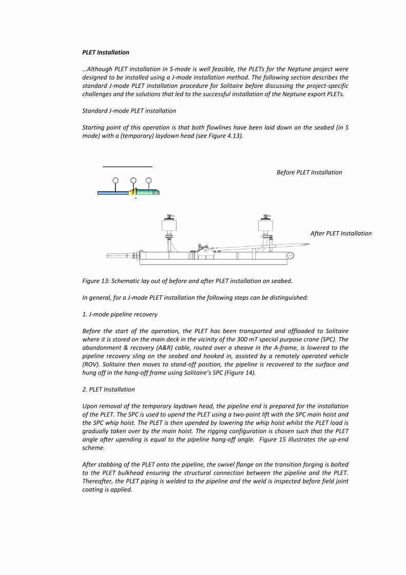
PLET Installation …Although PLET installation in S‐mode is well feasible, the PLETs for the Neptune project were designed to be installed using a J‐mode installation method. The following section describes the standard J‐mode PLET installation procedure for Solitaire before discussing the project‐specific challenges and the solutions that led to the successful installation of the Neptune export PLETs. Standard J‐mode PLET installation Starting point of this operation is that both flowlines have been laid down on the seabed (in S mode) with a (temporary) laydown head (see Figure 4.13).
Figure 13: Schematic lay out of before and after PLET installation on seabed. In general, for a J‐mode PLET installation the following steps can be distinguished: 1. J‐mode pipeline recovery Before the start of the operation, the PLET has been transported and offloaded to Solitaire where it is stored on the main deck in the vicinity of the 300 mT special purpose crane (SPC). The abandonment & recovery (A&R) cable, routed over a sheave in the A‐frame, is lowered to the pipeline recovery sling on the seabed and hooked in, assisted by a remotely operated vehicle (ROV). Solitaire then moves to stand‐off position, the pipeline is recovered to the surface and hung off in the hang‐off frame using Solitaire’s SPC (Figure 14).
2. PLET Installation Upon removal of the temporary laydown head, the pipeline end is prepared for the installation of the PLET. The SPC is used to upend the PLET using a two‐point lift with the SPC main hoist and the SPC whip hoist. The PLET is then upended by lowering the whip hoist whilst the PLET load is gradually taken over by the main hoist. The rigging configuration is chosen such that the PLET angle after upending is equal to the pipeline hang‐off angle. Figure 15 illustrates the up‐end scheme. After stabbing of the PLET onto the pipeline, the swivel flange on the transition forging is bolted to the PLET bulkhead ensuring the structural connection between the pipeline and the PLET. Thereafter, the PLET piping is welded to the pipeline and the weld is inspected before field joint coating is applied.
Before PLET Installation
After PLET Installation
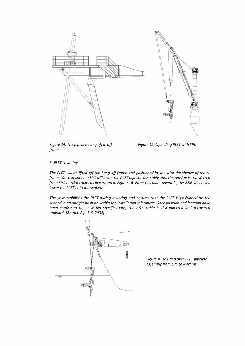
3. PLET Lowering The PLET will be lifted off the hang‐off frame and positioned in line with the sheave of the A‐frame. Once in line, the SPC will lower the PLET pipeline assembly until the tension is transferred from SPC to A&R cable, as illustrated in Figure 16. From this point onwards, the A&R winch will lower the PLET onto the seabed. The yoke stabilizes the PLET during lowering and ensures that the PLET is positioned on the seabed in an upright position within the installation tolerances. Once position and location have been confirmed to be within specifications, the A&R cable is disconnected and recovered onboard. [Antani, P.p. 5‐6, 2008].
Figure 14: The pipeline hung off in aft frame.
Figure 15: Upending PLET with SPC
Figure 4.16: Hand over PLET pipelineassembly from SPC to A‐frame
D.I.7 Workover and well intervention
Nergaard (Nergaard, 2009) give a definition of the two terms and explains its purposes as:
Workover: The term is used for a full overhaul of a well. It reflects the full capacity to change production equipment (tubing etc) in the well as well as the Xmas tree itself. This implies the use of a rig with fullbore BOP and marine riser. This means the we have to apply the same capacity systems as used during initial completion of the well. Full overhaul/workover might imply a full recompletion of the well. Using a full capacity drilling/completion rig offers the full capacity for redrilling, branch drilling and recompletion. In some cases we see the full capacity WOI system referred to as Category C intervention: heavy well intervention.
Well intervention: This term is used commonly for all vertical interventions that is done during the wells production life, ie after initial completion. The term is most commonly used for the lighter interventions; those implying that operations take place inside and through the Xmas tree and the tubing.
These are:
Category B intervention: medium well intervention, with smaller bore riser
Category A intervention: light well intervention – LWI, through water wireline operations..
The purpose of the interventions is increase the recovery rate and also as required:
• Survey – mapping status‐data gathering. • Change status (ex open/close zones – smart wells) • Repair • Measures for production stimulation.
D.I.8 Abandonment
At the end of the production life of the oilfield, the facilities must be decommissioned and abandoned according to the environmental and health requirements of the home country and any other applicable laws. The site must be restored to a condition that minimizes residual environmental impact and permits reinstatement of alternative industries in the area and unimpeded navigation through it.
• Floating production facilities will be removed from the field. • Subsea infrastructure must be removed or abandoned and the wells will be plugged and abandoned. • Buried flow lines must be abandoned at the place of the installation after be flushed.
D.II. Marine operations for a SPAR. The SPAR is a floating structure that typically involves complex marine operations; Reeg (Reeg et. al., 2000) provides a review of the installation process of the hull of the SPAR that is reproduced next:
Installation is performed in stages similar to those of other deepwater production systems, where one component is installed while another is being fabricated. Installation schedules heavily depend upon the completion status of the hull and topsides. Listed below are the order of events for a typical spar installation:
• Well predrilling (drilling vessel) • Export pipelines laying • Presite survey; transponder array deployment; anchor pile target buoys set • Anchor pile and mooring line settings • Hull delivery and upending • Temporary work deck setting • Mooring and pipeline attachment • Mooring lines pretensioning • Hull ballasting and removal of temporary work deck • Topsides delivery, installation, hookup, and integration • Buoyancy can installation
Prior to the delivery of the hull to location, a drilling rig might predrill one or more wells. (See figure 17) During this time, export pipelines are laid that will carry production either to another platform (host) or to shore after processing. A presite survey is performed and includes the following: onbottom acoustic array installed for the mooring system, identified obstructions removed, anchor pile target buoys preset, and a final survey of the mooring lay down area performed. Once on location, a derrick barge installs the anchor piles and mooring system. The installation of the anchor piles is performed using a deck‐mounted lowering system designed for deepwater installations and an underwater free‐riding hydraulic hammer with power pack. Remotely operated vehicles (ROV’s) observe the hammer and umbilical as the pile is lowered and stabbed into the seafloor. In conjunction with pile installation, the mooring system is laid out and temporarily abandoned. A wire deployment winch with reels specifically designed for this type of work handles each wire. An ROV monitors the wire lay‐down path as the derrick barge follows a predetermined route until it reaches the wire end on the deployment reel. The end of the mooring wire is then connected to an abandonment/recovery line and marked for later use in attaching the mooring system to the hull. To date, all GOM spar hulls have been built in Finland. Upon completion of the hull, it is shipped to the Gulf of Mexico on a heavy‐lift vessel such as the Mighty Servant III. See figure 18. Because of its size and length it is necessary to divide the spar hull into two sections. (NANSEN/BOMVANG were delivered in only one section) Upon arrival at an onshore facility, the sections are connected together using a wet mating technique, which allows for lower cost and ease of handling and positioning, and eliminates the need for special equipment. The hull is then ready for delivery to location.
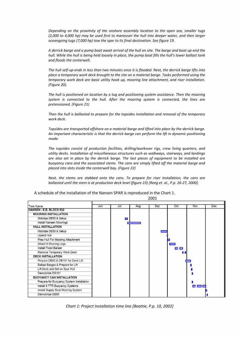
Depending on the proximity of the onshore assembly location to the open sea, smaller tugs (2,000 to 4,000 hp) may be used first to maneuver the hull into deeper water, and then larger oceangoing tugs (7,000 hp) tow the spar to its final destination. See figure 19. A derrick barge and a pump boat await arrival of the hull on site. The barge and boat up‐end the hull. While the hull is being held loosely in place, the pump boat fills the hull’s lower ballast tank and floods the centerwell. The hull self‐up‐ends in less than two minutes once it is flooded. Next, the derrick barge lifts into place a temporary work deck brought to the site on a material barge. Tasks performed using the temporary work deck are basic utility hook up, mooring line attachment, and riser installation. (Figure 20). The hull is positioned on location by a tug and positioning system assistance. Then the mooring system is connected to the hull. After the mooring system is connected, the lines are pretensioned. (Figure 21) Then the hull is ballasted to prepare for the topsides installation and removal of the temporary work deck. Topsides are transported offshore on a material barge and lifted into place by the derrick barge. An important characteristic is that the derrick barge can perform the lift in dynamic positioning mode. The topsides consist of production facilities, drilling/workover rigs, crew living quarters, and utility decks. Installation of miscellaneous structures such as walkways, stairways, and landings are also set in place by the derrick barge. The last pieces of equipment to be installed are buoyancy cans and the associated stems. The cans are simply lifted off the material barge and placed into slots inside the centerwell bay. (Figure 22) Next, the stems are stabbed onto the cans. To prepare for riser installation, the cans are ballasted until the stem is at production deck level (figure 23) [Reeg et. al., P.p. 26‐27, 2000].
A schedule of the installation of the Nansen SPAR is reproduced in the Chart 1. 2001
Chart 1: Project Installation time line [Beattie, P.p. 10, 2002]
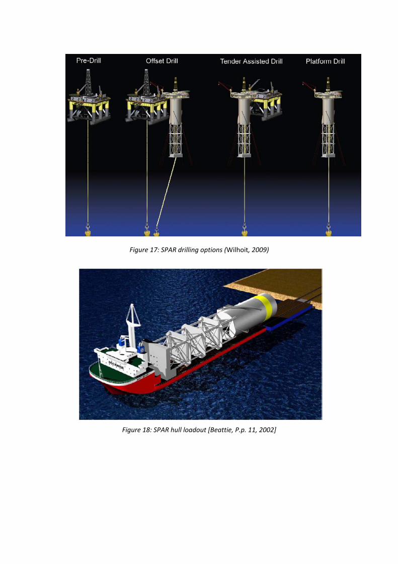
Figure 17: SPAR drilling options (Wilhoit, 2009)
Figure 18: SPAR hull loadout [Beattie, P.p. 11, 2002]
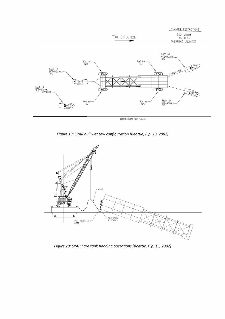
Figure 19: SPAR hull wet tow configuration [Beattie, P.p. 13, 2002]
Figure 20: SPAR hard tank flooding operations [Beattie, P.p. 13, 2002]
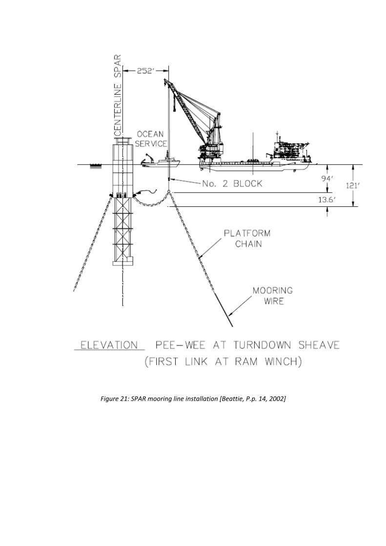
Figure 21: SPAR mooring line installation [Beattie, P.p. 14, 2002]
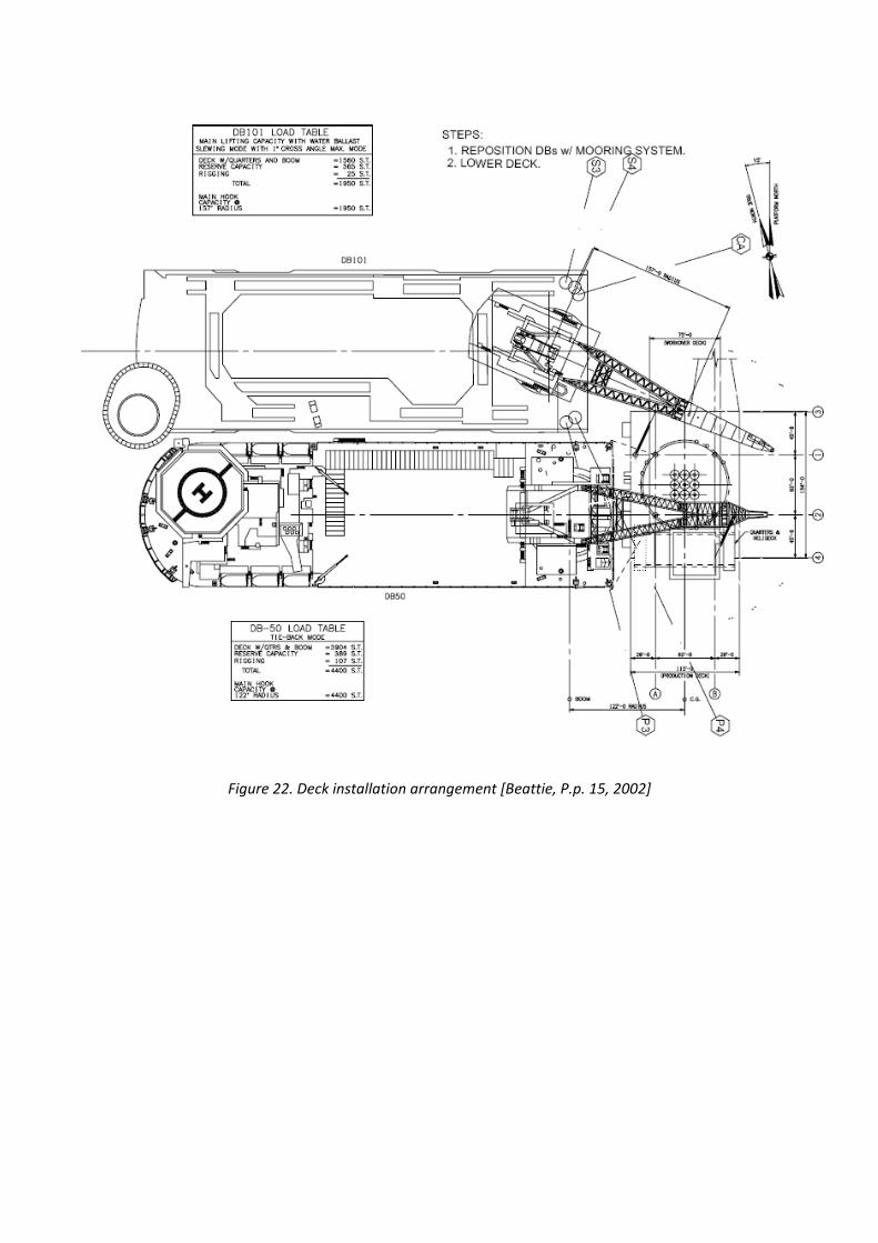
Figure 22. Deck installation arrangement [Beattie, P.p. 15, 2002]
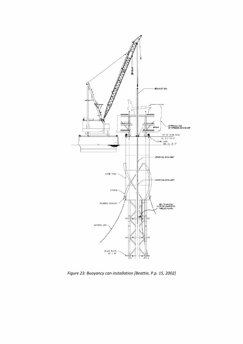
Figure 23: Buoyancy can installation [Beattie, P.p. 15, 2002]
D.III MARINE OPERATIONS FOR A TLP. Reeg et. al. resume the installation process of the TLP concepts that is reproduced next:
INSTALLATION OVERVIEW. Installation of a TLP is done in stages; often the design work on one section of the TLP is being done while another part is being installed. For example, the wells will often be predrilled while the TLP is being designed and constructed. Installation of a typical TLP is done in the following order: 1. Template for wells or foundation for TLP 2. Export pipelines 3. Flexible risers and mooring lines 4. Platform/Tendons 5. Hull and Surface Facility Template and Foundations Templates. Templates provide the layout for well locations and/or for the foundation, if needed. The wells may be drilled to their total depth, or partially drilled and the conductor casing set. Additional well drilling and completion operations can be done from the TLP. Template installation for drilling and foundation templates is similar, except some of the equipment used may be different. The template is built onshore and towed to location for installation. A drilling rig (mobile offshore drilling unit [MODU]) is preferred for installation because it eliminates the need for additional vessels. However, drilling rigs cannot lift large payloads and have limited lowering capacity. Large templates may need a crane for installation; they will also require costly handling systems and rigging. Foundations. Foundations secure the TLP to the seafloor by use of buried piles, which can be concrete or steel. Tendons are attached to the foundation and the platform is attached to the tendons. The piles can either be driven or drilled and grouted. Driven piles are expensive to install, but the holding power of drilled and grouted piles may not be as strong because of changes to the sole‐pile interface during the jetting and drilling operations. A typical vessel used for foundation installation would be one of the several available semisubmersible construction/crane vessels. A hydraulic hammer is used to drive the piles into the seafloor. Export Pipelines. Pipelines for the TLP are the same as pipelines used for conventional platforms. A steel catenary riser may be used to connect the subsea pipeline to the TLP. Various methods of installation can be used. The most common method used for installing pipelines is the J‐lay method. Pipelines for TLP’s range in size up to 18 inches in diameter for oil and approximately 14 inches for gas. Often the pipeline will join another system for transport to shore. Oil can be transported by tanker as an alternative to pipelines. Platform/Tendons. The TLP’s use tendons to secure the platform to the foundations. There is no set order for installation of the platform and tendons. In some cases the tendons will be connected to the foundations, and then the platform will be moved into place and the tendons secured to the platform. Other operations will move the platform in place first, secure the tendons to the platform, and then attach the tendons to the foundation. Another option is to secure some of the tendons to the foundations, move the platform in place, attach the secured tendons, and attach the remaining tendons to the TLP and then to the foundation. Hull and Surface Facility. The upper section of a TLP consists of the hull, the deck, and the surface facilities. The surface facility modules are built onshore and typically assembled at a
shallow‐water location near shore, then towed to the site. The modules may be attached to the hull either inshore or at the site. Economics are the determining factor for where the modules and hull are assembled. The hull provides the buoyancy for the TLP to float in the water and supports the platform. The hull contains several of the mechanical systems needed for platform operation. Topsides‐related equipment includes firewater, seawater, diesel storage, low toxic oil storage, and completion fluid storage systems. Hull‐related equipment includes ballasting and trim, drain and bilge 12 hours. • The platform was then transported to the site using four ocean‐going tugboats, traveling at three miles per hour, taking seven days for the 400‐mile transport. • Because the installation took place inshore there was no need for extra helicopters, supply boats, and marine equipment, and offshore operations, quartering, and weather delays were greatly reduced. Peak manpower used during installation was 350 people. Drilling Information. Well drilling for the TLP often begins after well template installation. A TLP can have 50 well slots with provisions for satellite subsea well tiebacks. Predrilling involves using a mobile offshore drilling unit (drillship or semisubmersible) to batch drill and case the wells to a convenient depth, normally through the shallow water flow zone or other potential hazard. Predrilling may also be suspended just above the production zone. Some wells may be drilled to total depth and completed. The Sonat George Richardson semisubmersible drilling vessel is an example of the type of vessel used to predrill.
The Typhoon project was extensively documented in various OTC papers and other publication, chart 2 shows the project Schedule, pay particular attention to the points 47 to 57 in that chart. Figure 24 shows the concept of the Typhoon field, note that this field is entirely a subsea development, while the most of the operations will not be so different as the one applied for the subsea tiebacks to shore, the availability of facilities close to the wells in this way increase the capability of processing and distribution of oil and gas which increase at the end the recovery factor.
D.IV. Marine operations for a semisubmersible. From the tree concepts of floating structures shown in this report, the semisubmersible is the less demanding on complexity and number of marine operations since the topsides can be preinstalled before the final emplacement. The onshore operation to place the topsides over the hull is called “superlift”. The mooring of the hull and the installation of risers and umbilicals to the main host are however operations that need to be carefully planned and is not less complex the translation from the construction yards to the field. The Na kika project was documented in those aspects in several papers:
• OTC 16701 Na Kika – Host Construction for Record Water Depth Platform. • OTC 16702 Na Kika – Deepwater Mooring and Host Installation. • OTC 16704 Na Kika Umbilical Transport & Installation Challenges. • OTC 16703 Design and Installation of the Na Kika Export Pipelines, Flowlines and
Risers.
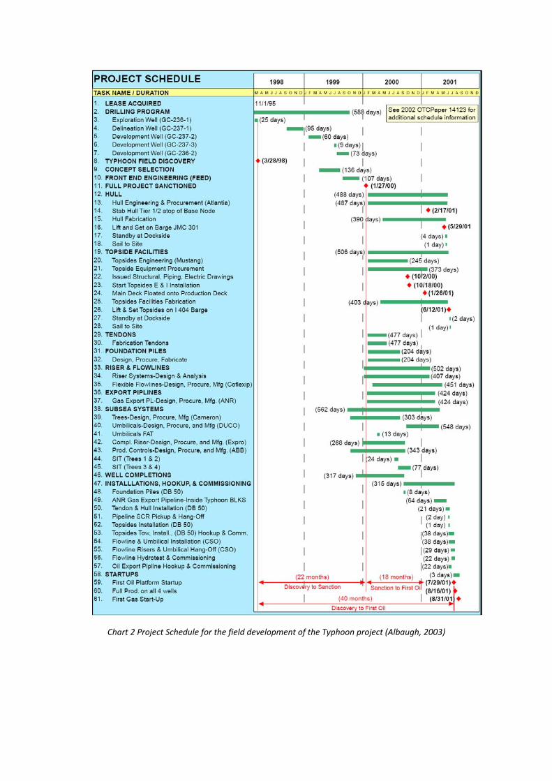
Chart 2 Project Schedule for the field development of the Typhoon project (Albaugh, 2003)
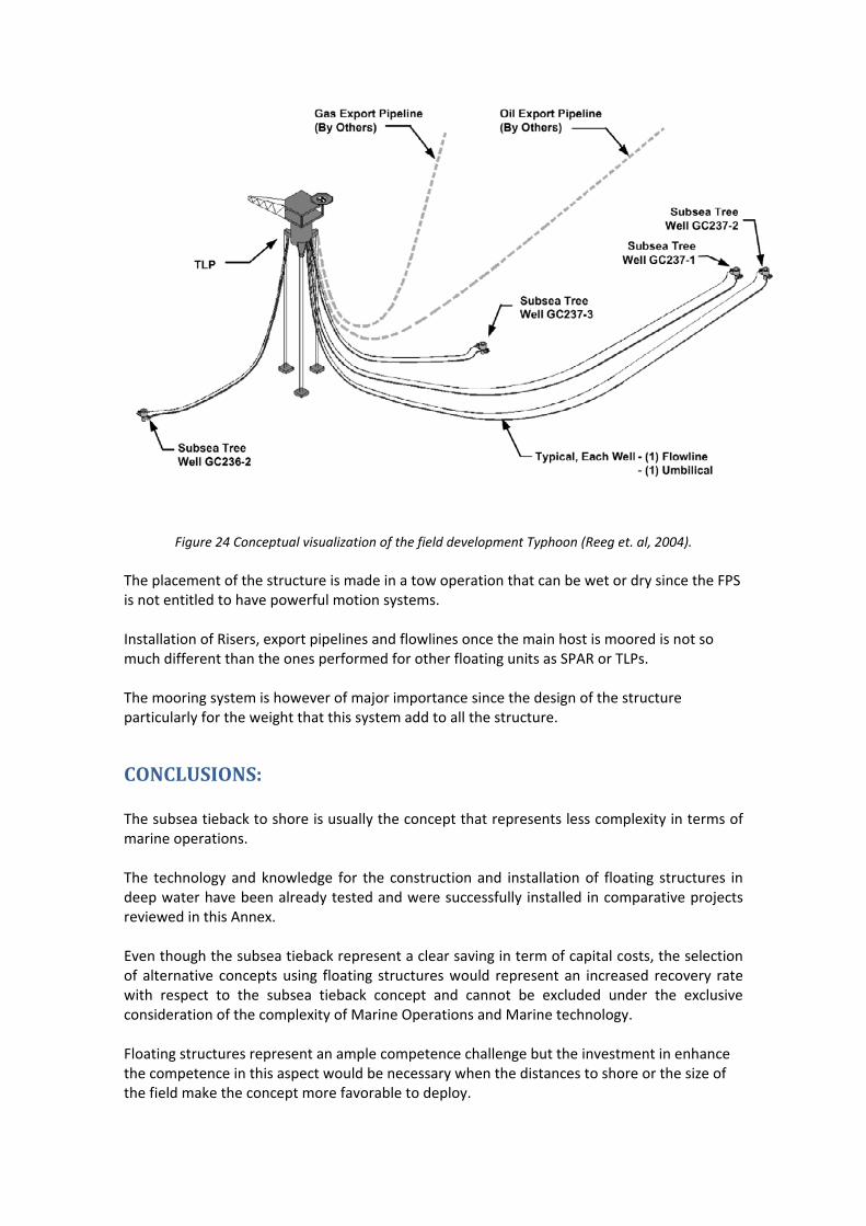
Figure 24 Conceptual visualization of the field development Typhoon (Reeg et. al, 2004). The placement of the structure is made in a tow operation that can be wet or dry since the FPS is not entitled to have powerful motion systems. Installation of Risers, export pipelines and flowlines once the main host is moored is not so much different than the ones performed for other floating units as SPAR or TLPs. The mooring system is however of major importance since the design of the structure particularly for the weight that this system add to all the structure.
CONCLUSIONS: The subsea tieback to shore is usually the concept that represents less complexity in terms of marine operations. The technology and knowledge for the construction and installation of floating structures in deep water have been already tested and were successfully installed in comparative projects reviewed in this Annex. Even though the subsea tieback represent a clear saving in term of capital costs, the selection of alternative concepts using floating structures would represent an increased recovery rate with respect to the subsea tieback concept and cannot be excluded under the exclusive consideration of the complexity of Marine Operations and Marine technology. Floating structures represent an ample competence challenge but the investment in enhance the competence in this aspect would be necessary when the distances to shore or the size of the field make the concept more favorable to deploy.
REFERENCES:
1. Albaugh E.K., Howell G., Lewis M & Autin M. BHPBilliton Petroleum (Americas), “TYPHOON FIELD DEVELOPMENT PROJECT Green Canyon Blocks 236 & 237”, Offshore Magazine Volume 63, Issue 2, February, USA, 2003.
2. Antani J. K., Enbridge Offshore Pipelines LLC, Dick W. T., Enbridge Offshore Pipelines LLC, Balch D., Pegasus International Inc, van der Leij T., Allseas USA Inc. “Design, Fabrication and Installation of the Neptune Export Lateral PLETs” Paper OTC 19668, Offshore Technology Conference, 2008.
3. Beattie S.M., Kerr‐McGee Oil & Gas Corporation; Pyles S., Kerr‐McGee Oil & Gas
Corporation; McCandless C. R., J. Ray McDermott, Inc.; Kuuri J., CSO Aker Rauma Offshore “Nansen/Boomvang Field Development – Construction and Installation” Paper OTC 14092, Offshore Technology Conference, 2002.
4. DCLG, Department for Communities and Local Government, Marine Mineral Guidance 1: Extraction by dredging from the English seabed, London, Uk, July 2002, consulted on internet, 8 november 2009, at http://www.communities.gov.uk/documents/planningandbuilding/pdf/156357.pdf
5. DNV, Det Norske Veritas “Rules for Planning and Execution of Marine Operations”, 2008.
6. FMC, FMC Technologies, “Subsea trees” online brochure, consulted on internet, 8 november 2009, at http://www.fmctechnologies.com/upload/subsea_tree_brochure.pdf
7. Gudmestad O.T. “Risk Assessment Tools for Use during Fabrication of Offshore Structures and in Marine Operations” Proceedings of OMAE01 20th International Conference on Offshore Mechanics and Arctic Engineering, Paper No. OMAE2001/S&R‐210,. June 3 ‐ 8, Rio de Janeiro, Brazil, 2001.
8. Gudmestad O.T., Bjerke P.E.; Statoil, “Uncertainties in weather forecasting, a risk to offshore operations” ISOPE Conference Vol. II P.p. 375‐380 Brest France, 1999.
9. Grenland, Grenland Group “References, subsea structures updated March 2008” online brochure, consulted on internet, 8 november 2009, at http://www.grenlandgroup.com/getfile.php/Filer/Attachments%20Subsea%20Fabrication/References%20Subsea%20Fabrication%20Updated%20March%202008.pdf
10. Homer S.T., Brown & Root Seaflo; Chitwood J.E., Chitwood Engineers; Childers T.W., Consultant; and Verrett A.J., Texaco E&P Inc. “Deepwater Templates and Cluster Well Manifolds: Is There a Single Correct Approach?” Paper OTC 7268, Offshore Technology Conference, 1993.
11. ISO‐13628‐1:2005 “Petroleum and natural gas industries — Design and operation of subsea production systems — Part 1: General requirements and recommendations” International Standard Organization, Switzerland, 2005.
12. Jan de Nul Group, Norfra Pipeline Project, Pretrenching, sea leveling and landfall dredging
and civil works, Brochure 1997. Consulted on internet , 8 november 2009, at http://www.kaminco.com/pdf/JanDeNul/NORWAY‐FRANCE%20NorFra.pdf
13. Komaromy S.M., Kearney J.P. Knight M.A., from Earl and Wight Ltd and Edwards W.G. from Humphreys & Glasgow Ltd “The design and installation of multiwell subsea template structures”, Advances in Underwater Technology. Ocean Science and Offshore Engineering, Volume II – Underwater Construction Development and Potential Society for Underwater Technology; Graham & Trotman, UK, 1987.
14. Nergaard, A. “Class Notes of Subsea Production Systems” University of Stavanger Compendium on it´s Learning, Norway, 2009.
15. Nogueira. A.C. Mckeehan D.S. INTEC Enginnering, “Design and construction of Offshore Pipelines ” Handbook of Offshore Engineering Edited by Chakrabarti S, U.S.A. 2005.
16. Petrobras, Petrobras America, “Cottonwood Field Development Project” February 2007. Consulted on internet , 8 november 2009, at http://www.petrobras‐usa.com/cottonwood/Cottonwood_Field_Development_February_2007.pdf
17. Petromena ASA, Information memorandum prepared in connection with the acquisition of the drilling rig SS Petrolia, Information Memorandum has been approved in accordance with the Continuing Obligations for companies listed on Oslo Axess; section 3.5.5.1., 7 November 2007. Consulted on internet, 8 november 2009, at http://www.petromena.no/docs/071107%20‐%20Petromena_Informasjonsdokument.pdf
18. POL, 1, Petroleum Open Learning, Unit 6 Floating Drilling Installations, Oilwell Drilling Technologies, United Kingdom, 2002.
19. POL, 2, Petroleum Open Learning, Unit 6 Subsea completions, Oilwell Production Technologies, United Kingdom, 2002.
20. Regg J.B., Atkins S., Hauser W., Hennessey J., Kruse B.J., Lowenhaupt J., Smith B., White A. “Deepwater Development: A Reference Document for the Deepwater Environmental Assessment Gulf of Mexico OCS (1998 through 2007)” MMS‐OCS, U.S. Department of the Interior Minerals Management Service Gulf of Mexico OCS Regional Office, New Orleans, USA, 2000.
21. Ruinen Ir. R.M, Application Engineer, Vryhof Anchors BV, “The use of drag embedment anchors in offshore mooring systems” Krimpen aan den IJssel, The Netherlands, 2003.
22. Visual dictionary Online, search by category HOME :: TRANSPORT & MACHINERY :: MARITIME TRANSPORT :: EXAMPLES OF BOATS AND SHIPS :: DRILL SHIP. Consulted on internet , 8 november 2009, at http://visual.merriam‐webster.com/transport‐machinery/maritime‐transport/examples‐boats‐ships/drill‐

ship.php&h=384&w=550&sz=59&tbnid=2QMzAT‐amilOsM:&tbnh=93&tbnw=133&prev=/images%3Fq%3Ddrilling%2Bship&hl=en&usg=__Snm0NIuSZLuDWdDNEeVbbvxTt2E=&ei=ukf5SqGnBI744AbM6c2_Cw&sa=X&oi=image_result&resnum=1&ct=image&ved=0CAcQ9QEwAA
23. Wilhoit L. and Supan C. Mustang Engineering. “2009 Worldwide survey of SPAR, DDCV and Min Doc vessels”, Offshore Magazine Volume 69, Issue 1, January, USA, 2009.
24. Wikipedia, Dynamic positioning, From Wikipedia, the free encyclopedia Consulted on internet , 8 november 2009, at http://en.wikipedia.org/wiki/Dynamic_positioning.
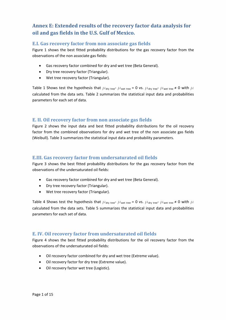
Page 1 of 15
Annex E: Extended results of the recovery factor data analysis for oil and gas fields in the U.S. Gulf of Mexico.
E.I. Gas recovery factor from non associate gas fields Figure 1 shows the best fitted probability distributions for the gas recovery factor from the observations of the non associate gas fields:
• Gas recovery factor combined for dry and wet tree (Beta General).
• Dry tree recovery factor (Triangular).
• Wet tree recovery factor (Triangular).
Table 1 Shows test the hypothesis that mdry tree‐ mwet tree = 0 vs. mdry tree‐ mwet tree ≠ 0 with m
calculated from the data sets. Table 2 summarizes the statistical input data and probabilities parameters for each set of data.
E. II. Oil recovery factor from non associate gas fields Figure 2 shows the input data and best fitted probability distributions for the oil recovery factor from the combined observations for dry and wet tree of the non associate gas fields (Weibull). Table 3 summarizes the statistical input data and probability parameters.
E.III. Gas recovery factor from undersaturated oil fields Figure 3 shows the best fitted probability distributions for the gas recovery factor from the observations of the undersaturated oil fields:
• Gas recovery factor combined for dry and wet tree (Beta General).
• Dry tree recovery factor (Triangular).
• Wet tree recovery factor (Triangular).
Table 4 Shows test the hypothesis that mdry tree‐ mwet tree = 0 vs. mdry tree‐ mwet tree ≠ 0 with m
calculated from the data sets. Table 5 summarizes the statistical input data and probabilities parameters for each set of data.
E. IV. Oil recovery factor from undersaturated oil fields Figure 4 shows the best fitted probability distributions for the oil recovery factor from the observations of the undersaturated oil fields:
• Oil recovery factor combined for dry and wet tree (Extreme value).
• Oil recovery factor for dry tree (Extreme value).
• Oil recovery factor wet tree (Logistic).
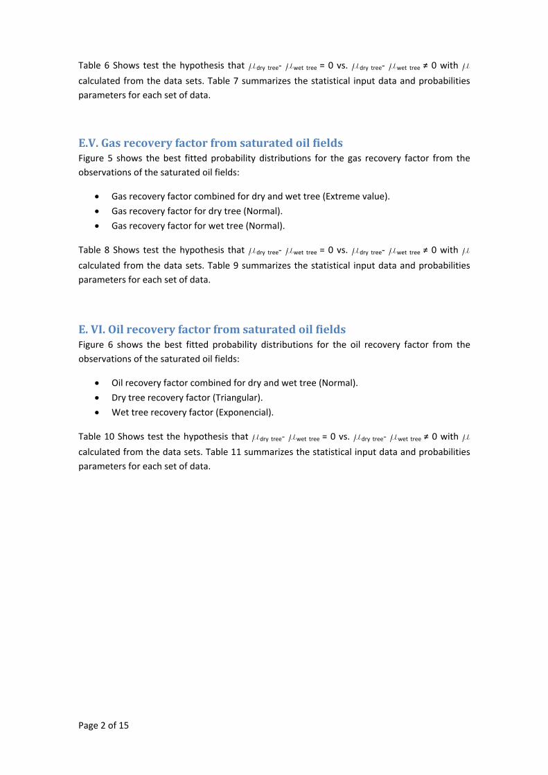
Page 2 of 15
Table 6 Shows test the hypothesis that mdry tree‐ mwet tree = 0 vs. mdry tree‐ mwet tree ≠ 0 with m
calculated from the data sets. Table 7 summarizes the statistical input data and probabilities parameters for each set of data.
E.V. Gas recovery factor from saturated oil fields Figure 5 shows the best fitted probability distributions for the gas recovery factor from the observations of the saturated oil fields:
• Gas recovery factor combined for dry and wet tree (Extreme value).
• Gas recovery factor for dry tree (Normal).
• Gas recovery factor for wet tree (Normal).
Table 8 Shows test the hypothesis that mdry tree‐ mwet tree = 0 vs. mdry tree‐ mwet tree ≠ 0 with m
calculated from the data sets. Table 9 summarizes the statistical input data and probabilities parameters for each set of data.
E. VI. Oil recovery factor from saturated oil fields Figure 6 shows the best fitted probability distributions for the oil recovery factor from the observations of the saturated oil fields:
• Oil recovery factor combined for dry and wet tree (Normal).
• Dry tree recovery factor (Triangular).
• Wet tree recovery factor (Exponencial).
Table 10 Shows test the hypothesis that mdry tree‐ mwet tree = 0 vs. mdry tree‐ mwet tree ≠ 0 with m
calculated from the data sets. Table 11 summarizes the statistical input data and probabilities parameters for each set of data.
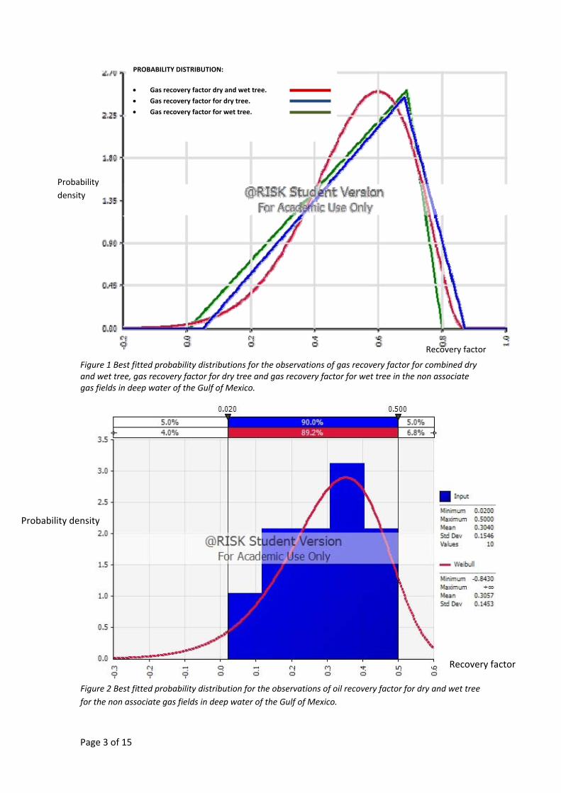
Page 3 of 15
Figure 1 Best fitted probability distributions for the observations of gas recovery factor for combined dry and wet tree, gas recovery factor for dry tree and gas recovery factor for wet tree in the non associate gas fields in deep water of the Gulf of Mexico. Figure 2 Best fitted probability distribution for the observations of oil recovery factor for dry and wet tree for the non associate gas fields in deep water of the Gulf of Mexico.
PROBABILITY DISTRIBUTION:
• Gas recovery factor dry and wet tree.
• Gas recovery factor for dry tree.
• Gas recovery factor for wet tree.
Recovery factor
Probability density
Probability density
Recovery factor
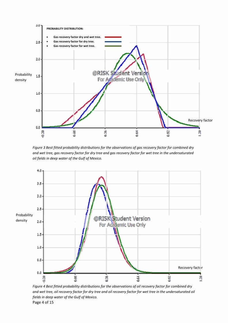
Page 4 of 15
Figure 3 Best fitted probability distributions for the observations of gas recovery factor for combined dry and wet tree, gas recovery factor for dry tree and gas recovery factor for wet tree in the undersaturated oil fields in deep water of the Gulf of Mexico.
Figure 4 Best fitted probability distributions for the observations of oil recovery factor for combined dry and wet tree, oil recovery factor for dry tree and oil recovery factor for wet tree in the undersaturated oil fields in deep water of the Gulf of Mexico.
Recovery factor
Probability density
PROBABILITY DISTRIBUTION:
• Gas recovery factor dry and wet tree.
• Gas recovery factor for dry tree.
• Gas recovery factor for wet tree.
Recovery factor
Probability density
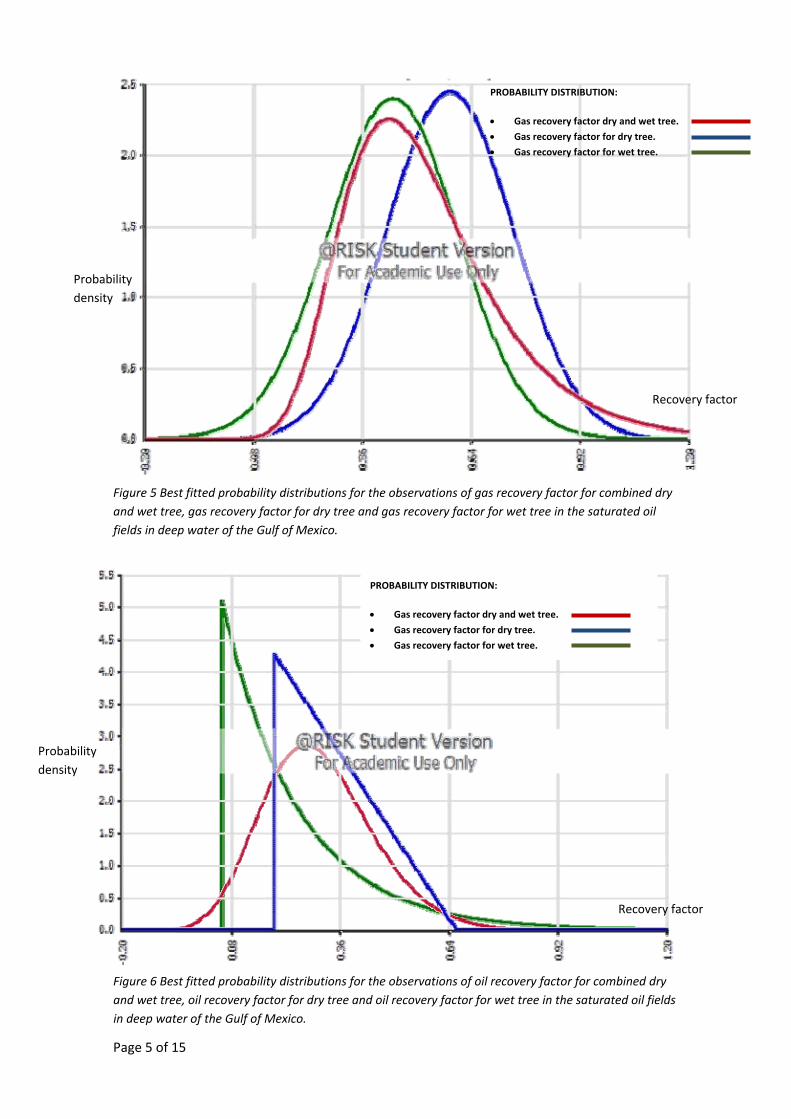
Page 5 of 15
Figure 5 Best fitted probability distributions for the observations of gas recovery factor for combined dry and wet tree, gas recovery factor for dry tree and gas recovery factor for wet tree in the saturated oil fields in deep water of the Gulf of Mexico.
Figure 6 Best fitted probability distributions for the observations of oil recovery factor for combined dry and wet tree, oil recovery factor for dry tree and oil recovery factor for wet tree in the saturated oil fields in deep water of the Gulf of Mexico.
Recovery factor
Probability density
PROBABILITY DISTRIBUTION:
• Gas recovery factor dry and wet tree.
• Gas recovery factor for dry tree.
• Gas recovery factor for wet tree.
Recovery factor
Probability density
PROBABILITY DISTRIBUTION:
• Gas recovery factor dry and wet tree.
• Gas recovery factor for dry tree.
• Gas recovery factor for wet tree.
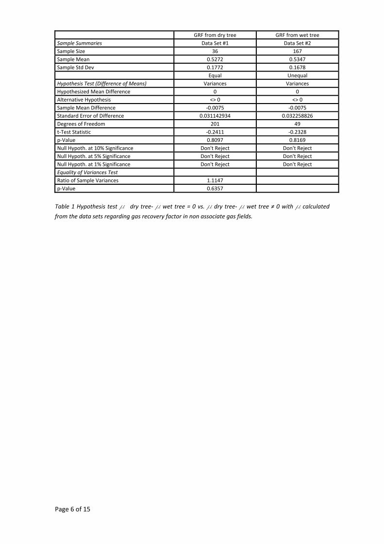
Page 6 of 15
GRF from dry tree GRF from wet tree
Sample Summaries Data Set #1 Data Set #2 Sample Size 36 167 Sample Mean 0.5272 0.5347 Sample Std Dev 0.1772 0.1678
Equal Unequal Hypothesis Test (Difference of Means) Variances Variances Hypothesized Mean Difference 0 0 Alternative Hypothesis <> 0 <> 0 Sample Mean Difference ‐0.0075 ‐0.0075 Standard Error of Difference 0.031142934 0.032258826 Degrees of Freedom 201 49 t‐Test Statistic ‐0.2411 ‐0.2328 p‐Value 0.8097 0.8169 Null Hypoth. at 10% Significance Don't Reject Don't Reject Null Hypoth. at 5% Significance Don't Reject Don't Reject Null Hypoth. at 1% Significance Don't Reject Don't Reject Equality of Variances Test Ratio of Sample Variances 1.1147 p‐Value 0.6357
Table 1 Hypothesis test m dry tree‐ m wet tree = 0 vs. m dry tree‐ m wet tree ≠ 0 with m calculated
from the data sets regarding gas recovery factor in non associate gas fields.
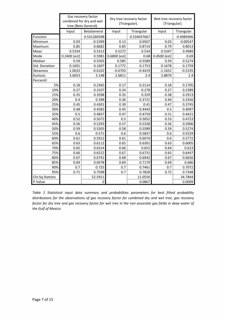
Page 7 of 15
Gas recovery factor combined for dry and wet
tree (Beta General).
Dry tree recovery factor (Triangular).
Wet tree recovery factor (Triangular).
Input BetaGeneral Input Triangular Input Triangular
Function 0.531260598 0.534037667 0.4989306Minimum 0.03 ‐0.5399 0.13 0.0507 0.03 0.00547Maximum 0.85 0.8682 0.85 0.8714 0.79 0.8013Mean 0.5334 0.5313 0.5272 0.534 0.5347 0.4989Mode 0.2400 [est] 0.5981 0.6800 [est] 0.68 0.4500 [est] 0.69Median 0.59 0.5505 0.585 0.5589 0.59 0.5274Std. Deviation 0.1691 0.1607 0.1772 0.1753 0.1678 0.1759Skewness ‐1.0633 ‐0.6102 ‐0.6703 ‐0.4419 ‐1.1652 ‐0.5235Kurtosis 3.6053 3.148 2.6811 2.4 3.8879 2.4Percentil
5% 0.18 0.2365 0.17 0.2114 0.18 0.170510% 0.27 0.3107 0.24 0.278 0.27 0.238915% 0.35 0.3598 0.35 0.329 0.38 0.291320% 0.4 0.398 0.36 0.3721 0.44 0.335625% 0.45 0.4301 0.39 0.41 0.47 0.374530% 0.48 0.4582 0.45 0.4443 0.5 0.409735% 0.5 0.4837 0.47 0.4759 0.51 0.442140% 0.52 0.5072 0.5 0.5052 0.53 0.472345% 0.56 0.5293 0.57 0.5328 0.56 0.500650% 0.59 0.5505 0.58 0.5589 0.59 0.527455% 0.6 0.571 0.6 0.5837 0.6 0.552960% 0.61 0.5912 0.61 0.6074 0.6 0.577265% 0.63 0.6112 0.65 0.6301 0.63 0.600570% 0.65 0.6314 0.66 0.652 0.64 0.62375% 0.66 0.6522 0.67 0.6731 0.65 0.644780% 0.67 0.6741 0.68 0.6942 0.67 0.665685% 0.69 0.6978 0.69 0.7179 0.69 0.68690% 0.7 0.725 0.7 0.7461 0.7 0.707295% 0.71 0.7598 0.7 0.7828 0.72 0.7348
Chi‐Sq Statistic 52.5911 11.0556 34.7844P‐Value 0 0.0867 0.0009
Table 2 Statistical input data summary and probabilities parameters for best fitted probability distributions for the observations of gas recovery factor for combined dry and wet tree, gas recovery factor for dry tree and gas recovery factor for wet tree in the non associate gas fields in deep water of the Gulf of Mexico.
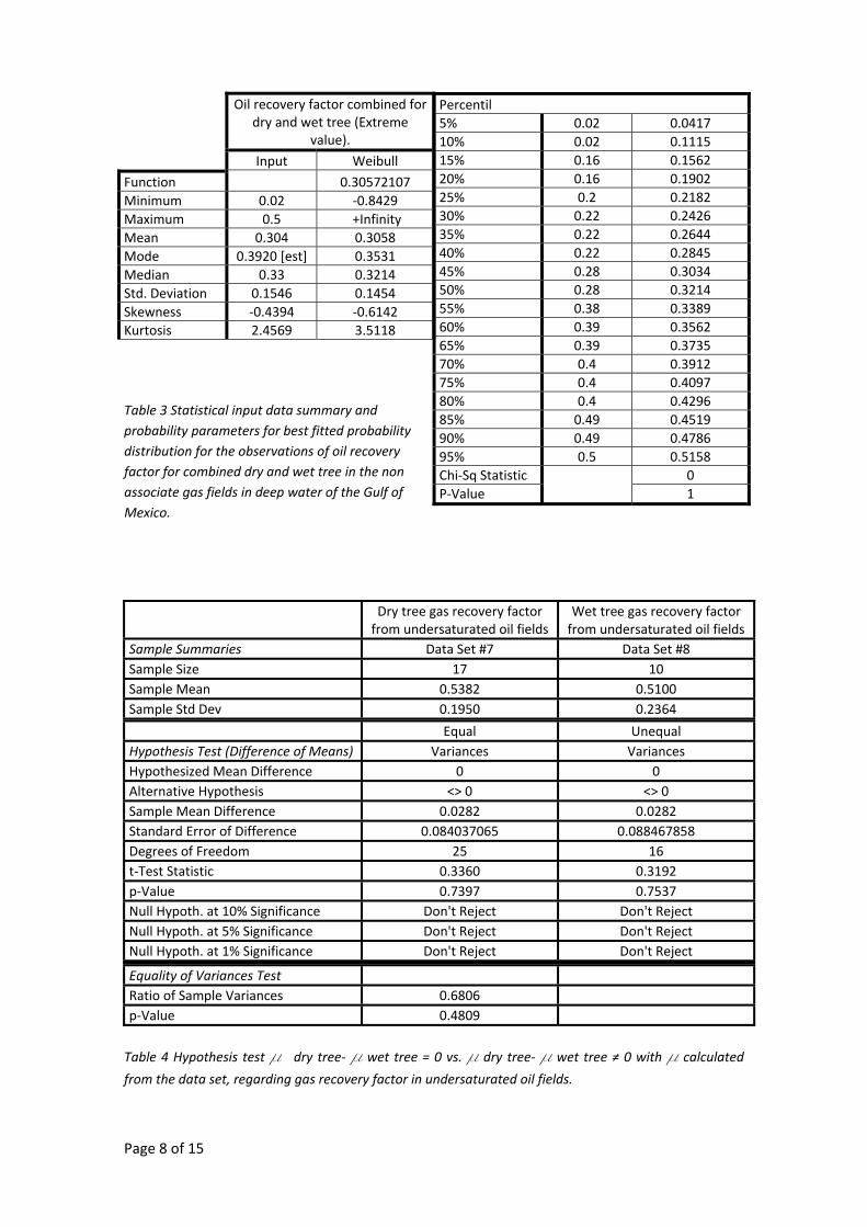
Page 8 of 15
Table 3 Statistical input data summary and probability parameters for best fitted probability distribution for the observations of oil recovery factor for combined dry and wet tree in the non associate gas fields in deep water of the Gulf of Mexico.
Dry tree gas recovery factor from undersaturated oil fields
Wet tree gas recovery factor from undersaturated oil fields
Sample Summaries Data Set #7 Data Set #8 Sample Size 17 10 Sample Mean 0.5382 0.5100 Sample Std Dev 0.1950 0.2364
Equal Unequal Hypothesis Test (Difference of Means) Variances Variances Hypothesized Mean Difference 0 0 Alternative Hypothesis <> 0 <> 0 Sample Mean Difference 0.0282 0.0282 Standard Error of Difference 0.084037065 0.088467858 Degrees of Freedom 25 16 t‐Test Statistic 0.3360 0.3192 p‐Value 0.7397 0.7537 Null Hypoth. at 10% Significance Don't Reject Don't Reject Null Hypoth. at 5% Significance Don't Reject Don't Reject Null Hypoth. at 1% Significance Don't Reject Don't Reject
Equality of Variances Test Ratio of Sample Variances 0.6806p‐Value 0.4809
Table 4 Hypothesis test m dry tree‐ m wet tree = 0 vs. m dry tree‐ m wet tree ≠ 0 with m calculated
from the data set, regarding gas recovery factor in undersaturated oil fields.
Oil recovery factor combined for dry and wet tree (Extreme
value).
Input Weibull
Function 0.30572107Minimum 0.02 ‐0.8429Maximum 0.5 +InfinityMean 0.304 0.3058Mode 0.3920 [est] 0.3531Median 0.33 0.3214Std. Deviation 0.1546 0.1454Skewness ‐0.4394 ‐0.6142Kurtosis 2.4569 3.5118
Percentil 5% 0.02 0.0417 10% 0.02 0.1115 15% 0.16 0.1562 20% 0.16 0.1902 25% 0.2 0.2182 30% 0.22 0.2426 35% 0.22 0.2644 40% 0.22 0.2845 45% 0.28 0.3034 50% 0.28 0.3214 55% 0.38 0.3389 60% 0.39 0.3562 65% 0.39 0.3735 70% 0.4 0.3912 75% 0.4 0.4097 80% 0.4 0.4296 85% 0.49 0.4519 90% 0.49 0.4786 95% 0.5 0.5158 Chi‐Sq Statistic 0 P‐Value 1
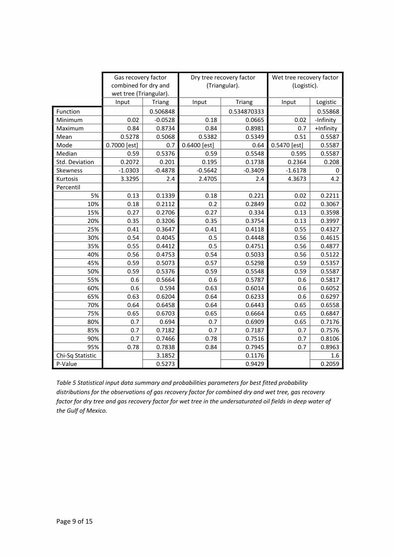
Page 9 of 15
Gas recovery factor combined for dry and wet tree (Triangular).
Dry tree recovery factor (Triangular).
Wet tree recovery factor (Logistic).
Input Triang Input Triang Input Logistic
Function 0.506848 0.534870333 0.55868Minimum 0.02 ‐0.0528 0.18 0.0665 0.02 ‐InfinityMaximum 0.84 0.8734 0.84 0.8981 0.7 +InfinityMean 0.5278 0.5068 0.5382 0.5349 0.51 0.5587Mode 0.7000 [est] 0.7 0.6400 [est] 0.64 0.5470 [est] 0.5587Median 0.59 0.5376 0.59 0.5548 0.595 0.5587Std. Deviation 0.2072 0.201 0.195 0.1738 0.2364 0.208Skewness ‐1.0303 ‐0.4878 ‐0.5642 ‐0.3409 ‐1.6178 0Kurtosis 3.3295 2.4 2.4705 2.4 4.3673 4.2Percentil
5% 0.13 0.1339 0.18 0.221 0.02 0.221110% 0.18 0.2112 0.2 0.2849 0.02 0.306715% 0.27 0.2706 0.27 0.334 0.13 0.359820% 0.35 0.3206 0.35 0.3754 0.13 0.399725% 0.41 0.3647 0.41 0.4118 0.55 0.432730% 0.54 0.4045 0.5 0.4448 0.56 0.461535% 0.55 0.4412 0.5 0.4751 0.56 0.487740% 0.56 0.4753 0.54 0.5033 0.56 0.512245% 0.59 0.5073 0.57 0.5298 0.59 0.535750% 0.59 0.5376 0.59 0.5548 0.59 0.558755% 0.6 0.5664 0.6 0.5787 0.6 0.581760% 0.6 0.594 0.63 0.6014 0.6 0.605265% 0.63 0.6204 0.64 0.6233 0.6 0.629770% 0.64 0.6458 0.64 0.6443 0.65 0.655875% 0.65 0.6703 0.65 0.6664 0.65 0.684780% 0.7 0.694 0.7 0.6909 0.65 0.717685% 0.7 0.7182 0.7 0.7187 0.7 0.757690% 0.7 0.7466 0.78 0.7516 0.7 0.810695% 0.78 0.7838 0.84 0.7945 0.7 0.8963
Chi‐Sq Statistic 3.1852 0.1176 1.6P‐Value 0.5273 0.9429 0.2059
Table 5 Statistical input data summary and probabilities parameters for best fitted probability distributions for the observations of gas recovery factor for combined dry and wet tree, gas recovery factor for dry tree and gas recovery factor for wet tree in the undersaturated oil fields in deep water of the Gulf of Mexico.
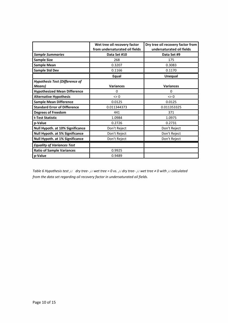
Page 10 of 15
Wet tree oil recovery factor from undersaturated oil fields
Dry tree oil recovery factor from undersaturated oil fields
Sample Summaries Data Set #10 Data Set #9 Sample Size 268 175 Sample Mean 0.3207 0.3083 Sample Std Dev 0.1166 0.1170
Equal Unequal Hypothesis Test (Difference of Means) Variances Variances Hypothesized Mean Difference 0 0 Alternative Hypothesis <> 0 <> 0 Sample Mean Difference 0.0125 0.0125 Standard Error of Difference 0.011344373 0.011353325 Degrees of Freedom 441 371 t‐Test Statistic 1.0984 1.0975 p‐Value 0.2726 0.2731 Null Hypoth. at 10% Significance Don't Reject Don't Reject Null Hypoth. at 5% Significance Don't Reject Don't Reject Null Hypoth. at 1% Significance Don't Reject Don't Reject
Equality of Variances Test Ratio of Sample Variances 0.9925p‐Value 0.9489
Table 6 Hypothesis test m dry tree‐ m wet tree = 0 vs. m dry tree‐ m wet tree ≠ 0 with m calculated
from the data set regarding oil recovery factor in undersaturated oil fields.
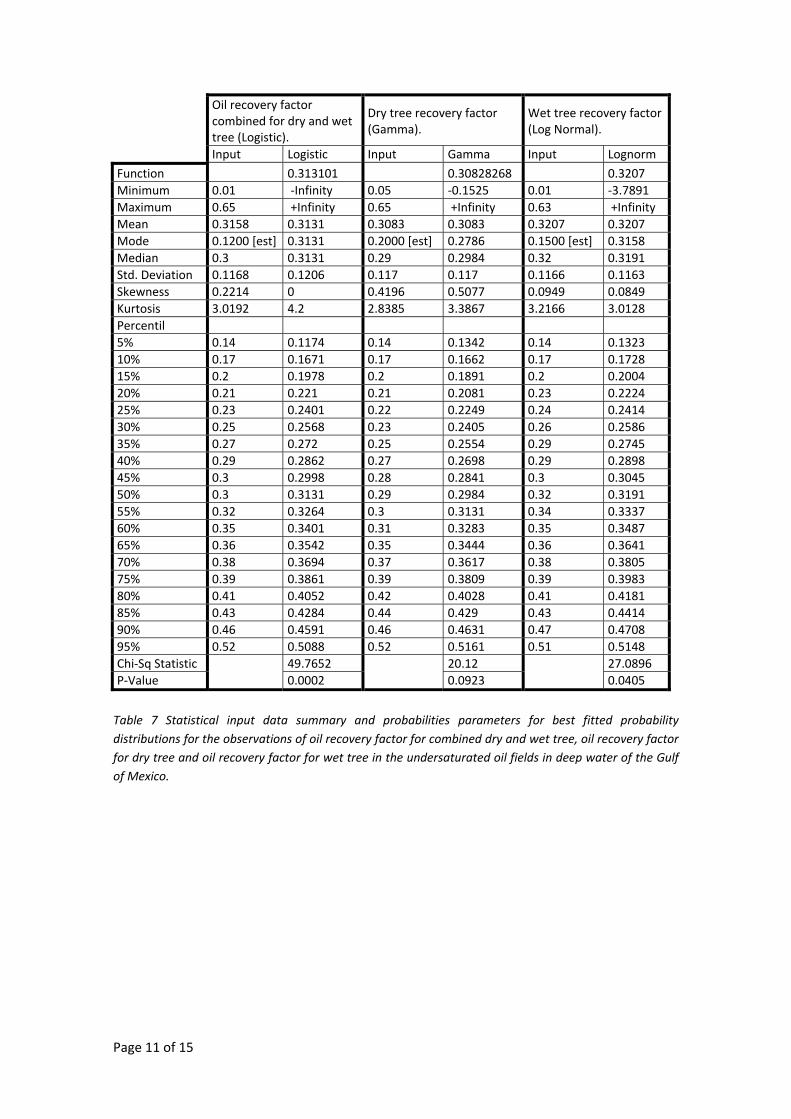
Page 11 of 15
Oil recovery factor combined for dry and wet tree (Logistic).
Dry tree recovery factor (Gamma).
Wet tree recovery factor (Log Normal).
Input Logistic Input Gamma Input Lognorm
Function 0.313101 0.30828268 0.3207 Minimum 0.01 ‐Infinity 0.05 ‐0.1525 0.01 ‐3.7891 Maximum 0.65 +Infinity 0.65 +Infinity 0.63 +InfinityMean 0.3158 0.3131 0.3083 0.3083 0.3207 0.3207 Mode 0.1200 [est] 0.3131 0.2000 [est] 0.2786 0.1500 [est] 0.3158 Median 0.3 0.3131 0.29 0.2984 0.32 0.3191 Std. Deviation 0.1168 0.1206 0.117 0.117 0.1166 0.1163 Skewness 0.2214 0 0.4196 0.5077 0.0949 0.0849 Kurtosis 3.0192 4.2 2.8385 3.3867 3.2166 3.0128 Percentil 5% 0.14 0.1174 0.14 0.1342 0.14 0.1323 10% 0.17 0.1671 0.17 0.1662 0.17 0.1728 15% 0.2 0.1978 0.2 0.1891 0.2 0.2004 20% 0.21 0.221 0.21 0.2081 0.23 0.2224 25% 0.23 0.2401 0.22 0.2249 0.24 0.2414 30% 0.25 0.2568 0.23 0.2405 0.26 0.2586 35% 0.27 0.272 0.25 0.2554 0.29 0.2745 40% 0.29 0.2862 0.27 0.2698 0.29 0.2898 45% 0.3 0.2998 0.28 0.2841 0.3 0.3045 50% 0.3 0.3131 0.29 0.2984 0.32 0.3191 55% 0.32 0.3264 0.3 0.3131 0.34 0.3337 60% 0.35 0.3401 0.31 0.3283 0.35 0.3487 65% 0.36 0.3542 0.35 0.3444 0.36 0.3641 70% 0.38 0.3694 0.37 0.3617 0.38 0.3805 75% 0.39 0.3861 0.39 0.3809 0.39 0.3983 80% 0.41 0.4052 0.42 0.4028 0.41 0.4181 85% 0.43 0.4284 0.44 0.429 0.43 0.4414 90% 0.46 0.4591 0.46 0.4631 0.47 0.4708 95% 0.52 0.5088 0.52 0.5161 0.51 0.5148 Chi‐Sq Statistic 49.7652 20.12 27.0896 P‐Value 0.0002 0.0923 0.0405
Table 7 Statistical input data summary and probabilities parameters for best fitted probability distributions for the observations of oil recovery factor for combined dry and wet tree, oil recovery factor for dry tree and oil recovery factor for wet tree in the undersaturated oil fields in deep water of the Gulf of Mexico.
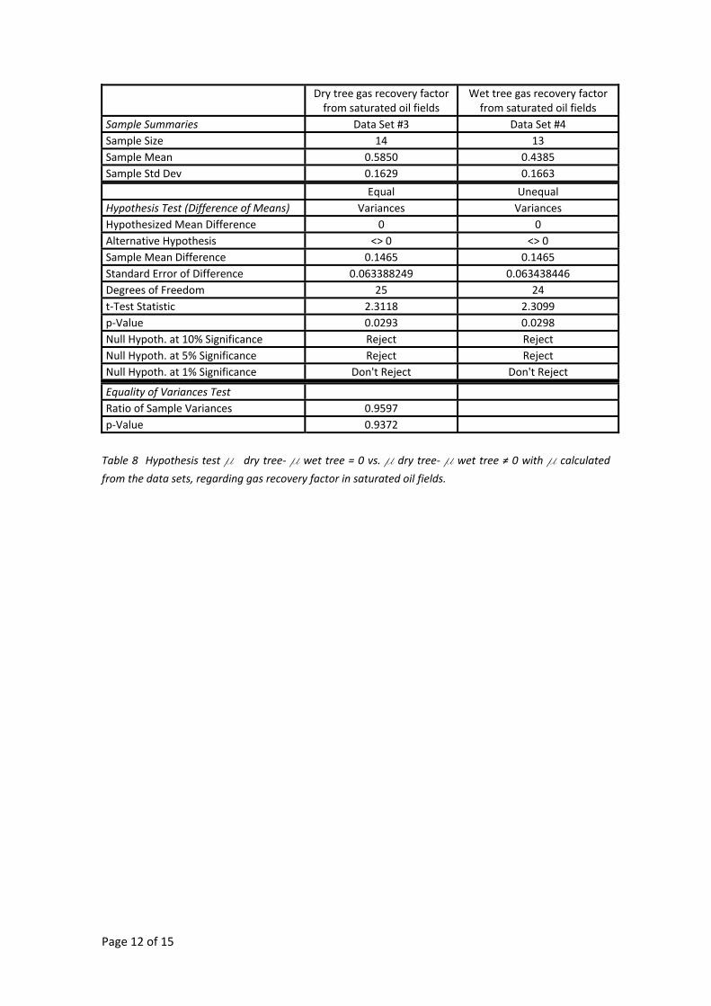
Page 12 of 15
Dry tree gas recovery factor from saturated oil fields
Wet tree gas recovery factor from saturated oil fields
Sample Summaries Data Set #3 Data Set #4 Sample Size 14 13 Sample Mean 0.5850 0.4385 Sample Std Dev 0.1629 0.1663
Equal Unequal Hypothesis Test (Difference of Means) Variances Variances Hypothesized Mean Difference 0 0 Alternative Hypothesis <> 0 <> 0 Sample Mean Difference 0.1465 0.1465 Standard Error of Difference 0.063388249 0.063438446 Degrees of Freedom 25 24 t‐Test Statistic 2.3118 2.3099 p‐Value 0.0293 0.0298 Null Hypoth. at 10% Significance Reject Reject Null Hypoth. at 5% Significance Reject Reject Null Hypoth. at 1% Significance Don't Reject Don't Reject
Equality of Variances Test Ratio of Sample Variances 0.9597p‐Value 0.9372
Table 8 Hypothesis test m dry tree‐ m wet tree = 0 vs. m dry tree‐ m wet tree ≠ 0 with m calculated
from the data sets, regarding gas recovery factor in saturated oil fields.
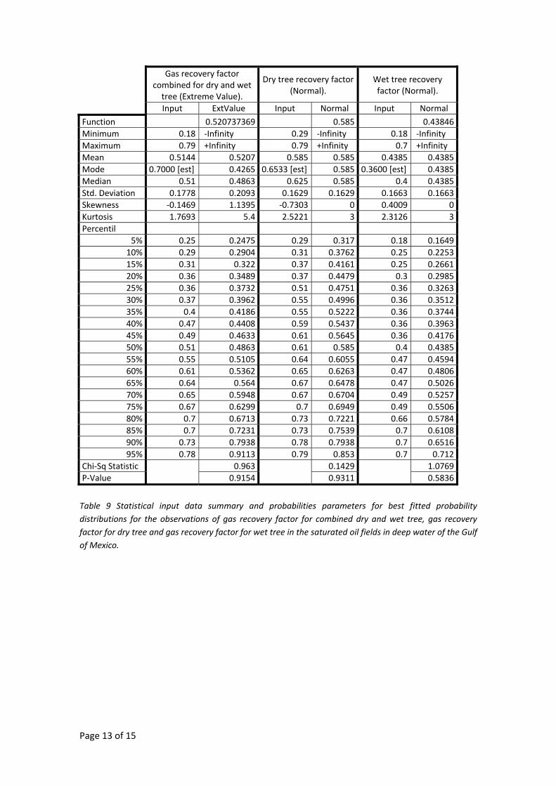
Page 13 of 15
Gas recovery factor combined for dry and wet tree (Extreme Value).
Dry tree recovery factor (Normal).
Wet tree recovery factor (Normal).
Input ExtValue Input Normal Input Normal
Function 0.520737369 0.585 0.43846 Minimum 0.18 ‐Infinity 0.29 ‐Infinity 0.18 ‐Infinity Maximum 0.79 +Infinity 0.79 +Infinity 0.7 +Infinity Mean 0.5144 0.5207 0.585 0.585 0.4385 0.4385 Mode 0.7000 [est] 0.4265 0.6533 [est] 0.585 0.3600 [est] 0.4385 Median 0.51 0.4863 0.625 0.585 0.4 0.4385 Std. Deviation 0.1778 0.2093 0.1629 0.1629 0.1663 0.1663 Skewness ‐0.1469 1.1395 ‐0.7303 0 0.4009 0 Kurtosis 1.7693 5.4 2.5221 3 2.3126 3 Percentil
5% 0.25 0.2475 0.29 0.317 0.18 0.1649 10% 0.29 0.2904 0.31 0.3762 0.25 0.2253 15% 0.31 0.322 0.37 0.4161 0.25 0.2661 20% 0.36 0.3489 0.37 0.4479 0.3 0.2985 25% 0.36 0.3732 0.51 0.4751 0.36 0.3263 30% 0.37 0.3962 0.55 0.4996 0.36 0.3512 35% 0.4 0.4186 0.55 0.5222 0.36 0.3744 40% 0.47 0.4408 0.59 0.5437 0.36 0.3963 45% 0.49 0.4633 0.61 0.5645 0.36 0.4176 50% 0.51 0.4863 0.61 0.585 0.4 0.4385 55% 0.55 0.5105 0.64 0.6055 0.47 0.4594 60% 0.61 0.5362 0.65 0.6263 0.47 0.4806 65% 0.64 0.564 0.67 0.6478 0.47 0.5026 70% 0.65 0.5948 0.67 0.6704 0.49 0.5257 75% 0.67 0.6299 0.7 0.6949 0.49 0.5506 80% 0.7 0.6713 0.73 0.7221 0.66 0.5784 85% 0.7 0.7231 0.73 0.7539 0.7 0.6108 90% 0.73 0.7938 0.78 0.7938 0.7 0.6516 95% 0.78 0.9113 0.79 0.853 0.7 0.712
Chi‐Sq Statistic 0.963 0.1429 1.0769 P‐Value 0.9154 0.9311 0.5836
Table 9 Statistical input data summary and probabilities parameters for best fitted probability distributions for the observations of gas recovery factor for combined dry and wet tree, gas recovery factor for dry tree and gas recovery factor for wet tree in the saturated oil fields in deep water of the Gulf of Mexico.
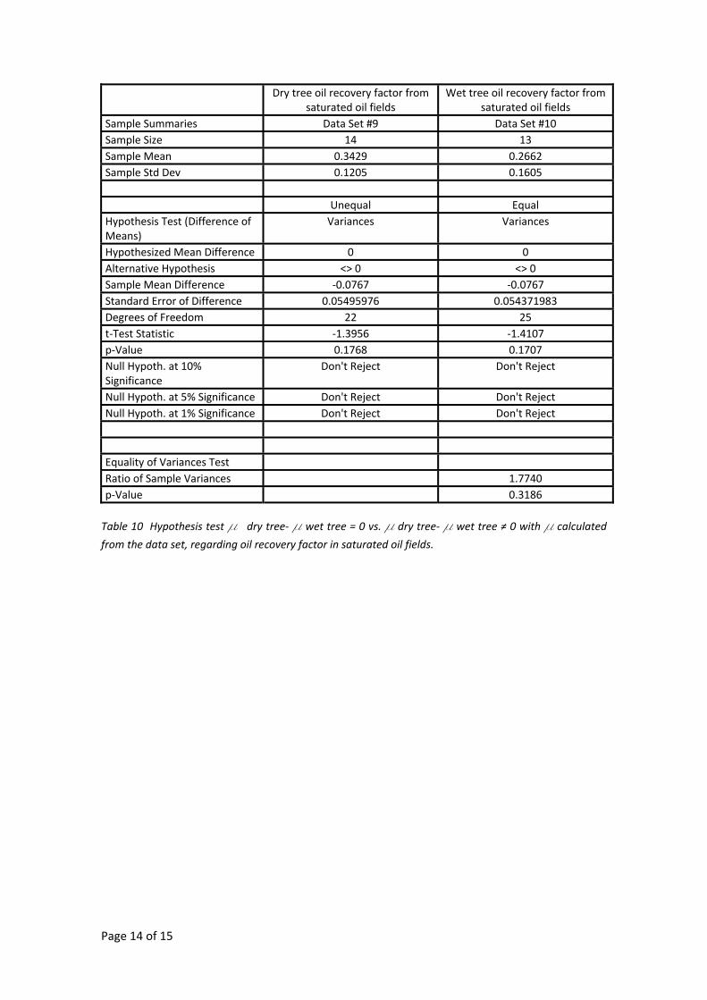
Page 14 of 15
Dry tree oil recovery factor from saturated oil fields
Wet tree oil recovery factor from saturated oil fields
Sample Summaries Data Set #9 Data Set #10 Sample Size 14 13 Sample Mean 0.3429 0.2662 Sample Std Dev 0.1205 0.1605 Unequal Equal Hypothesis Test (Difference of Means)
Variances Variances
Hypothesized Mean Difference 0 0 Alternative Hypothesis <> 0 <> 0 Sample Mean Difference ‐0.0767 ‐0.0767 Standard Error of Difference 0.05495976 0.054371983 Degrees of Freedom 22 25 t‐Test Statistic ‐1.3956 ‐1.4107 p‐Value 0.1768 0.1707 Null Hypoth. at 10% Significance
Don't Reject Don't Reject
Null Hypoth. at 5% Significance Don't Reject Don't Reject Null Hypoth. at 1% Significance Don't Reject Don't Reject Equality of Variances Test Ratio of Sample Variances 1.7740 p‐Value 0.3186 Table 10 Hypothesis test m dry tree‐ m wet tree = 0 vs. m dry tree‐ m wet tree ≠ 0 with m calculated
from the data set, regarding oil recovery factor in saturated oil fields.
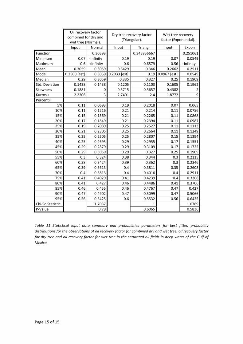
Page 15 of 15
Oil recovery factor combined for dry and wet tree (Normal).
Dry tree recovery factor (Triangular).
Wet tree recovery factor (Exponential).
Input Normal Input Triang Input Expon
Function 0.30593 0.345956667 0.251061 Minimum 0.07 ‐Infinity 0.19 0.19 0.07 0.0549 Maximum 0.6 +Infinity 0.6 0.6579 0.56 +Infinity Mean 0.3059 0.3059 0.3429 0.346 0.2662 0.2511 Mode 0.2500 [est] 0.3059 0.2033 [est] 0.19 0.0967 [est] 0.0549 Median 0.29 0.3059 0.335 0.327 0.25 0.1909 Std. Deviation 0.1438 0.1438 0.1205 0.1103 0.1605 0.1962 Skewness 0.1881 0 0.5715 0.5657 0.4382 2 Kurtosis 2.2206 3 2.7491 2.4 1.8772 9 Percentil
5% 0.11 0.0693 0.19 0.2018 0.07 0.065 10% 0.11 0.1216 0.21 0.214 0.11 0.0756 15% 0.15 0.1569 0.21 0.2265 0.11 0.0868 20% 0.17 0.1849 0.21 0.2394 0.11 0.0987 25% 0.19 0.2089 0.25 0.2527 0.11 0.1113 30% 0.21 0.2305 0.25 0.2664 0.11 0.1249 35% 0.25 0.2505 0.25 0.2807 0.15 0.1394 40% 0.25 0.2695 0.29 0.2955 0.17 0.1551 45% 0.29 0.2879 0.29 0.3109 0.17 0.1722 50% 0.29 0.3059 0.29 0.327 0.25 0.1909 55% 0.3 0.324 0.38 0.344 0.3 0.2115 60% 0.38 0.3424 0.39 0.362 0.3 0.2346 65% 0.39 0.3613 0.4 0.3811 0.35 0.2608 70% 0.4 0.3813 0.4 0.4016 0.4 0.2911 75% 0.41 0.4029 0.41 0.4239 0.4 0.3268 80% 0.41 0.427 0.46 0.4486 0.41 0.3706 85% 0.46 0.455 0.46 0.4767 0.47 0.427 90% 0.47 0.4902 0.47 0.5099 0.47 0.5066 95% 0.56 0.5425 0.6 0.5532 0.56 0.6425
Chi‐Sq Statistic 1.7037 1 1.0769 P‐Value 0.79 0.6065 0.5836
Table 11 Statistical input data summary and probabilities parameters for best fitted probability distributions for the observations of oil recovery factor for combined dry and wet tree, oil recovery factor for dry tree and oil recovery factor for wet tree in the saturated oil fields in deep water of the Gulf of Mexico.
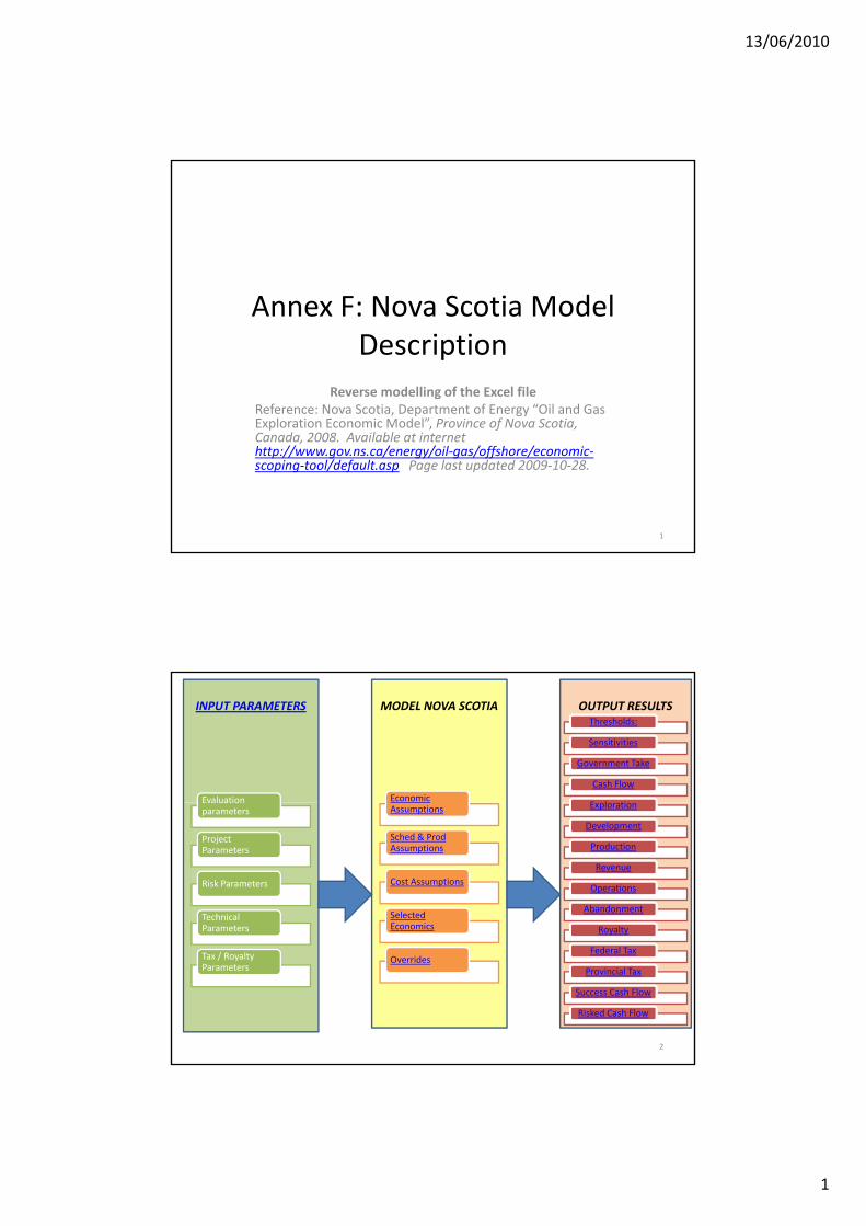
13/06/2010
1
Annex F: Nova Scotia ModelDescription
Reverse modelling of the Excel fileReference: Nova Scotia, Department of Energy “Oil and Gas Exploration Economic Model” Province of Nova ScotiaExploration Economic Model , Province of Nova Scotia, Canada, 2008. Available at internet http://www.gov.ns.ca/energy/oil‐gas/offshore/economic‐scoping‐tool/default.asp Page last updated 2009‐10‐28.
1
OUTPUT RESULTSINPUT PARAMETERS MODEL NOVA SCOTIAThresholds:
Sensitivities
Government Take
Cash Flow
E l tiEconomic Evaluation Exploration
Development
Production
Revenue
Operations
Abandonment
Royalty
Assumptions
Sched & Prod Assumptions
Cost Assumptions
Selected Economics
Evaluation parameters
Project Parameters
Risk Parameters
Technical Parameters y y
Federal Tax
Provincial Tax
Success Cash Flow
Risked Cash Flow
OverridesTax / Royalty Parameters
2
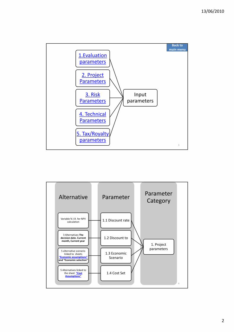
13/06/2010
2
1.Evaluation parameters
2. Project
Back tomain menu
Input parameters
Parameters
3. RiskParameters
4 Technical4. TechnicalParameters
5. Tax/Royalty parameters
3
Alternative Parameter ParameterCategory
1. Project parameters
1.1 Discount rateVariable % I.R. for NPV calculation
1.2 Discount to3 Alternatives The
decision date. Current month, Current year
1 3 Economic5 alternative scenario
1.3 EconomicScenario
linked to sheets “Economic assumptions” and “Economic selection”
1.4 Cost Set5 Alternatives linked to
the sheet “CostAssumptions”
4
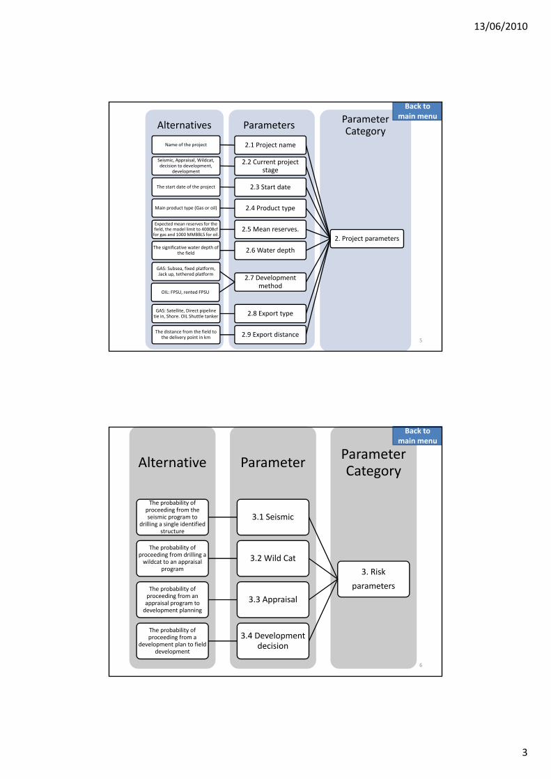
13/06/2010
3
ParameterCategory
2.1 Project nameName of the project
2.2 Current projectstage
Seismic, Appraisal, Wildcat, decision to development,
development
2 3 St t d tTh d f h j
ParametersAlternatives
Back tomain menu
2. Project parameters
2.3 Start dateThe start date of the project
2.4 Product typeMain product type (Gas or oil)
2.5 Mean reserves.Expected mean reserves for the field, the model limit to 4000Bcf for gas and 1000 MMBBLS for oil.
2.6 Water depthThe significative water depth of the field
GAS: Subsea fixed platform
2.7 Developmentmethod
GAS: Subsea, fixed platform, Jack up, tethered platform
OIL: FPSU, rented FPSU
2.8 Export typeGAS: Satellite, Direct pipeline tie in, Shore. OIL Shuttle tanker
2.9 Export distanceThe distance from the field to the delivery point in km
5
Alternative Parameter ParameterCategory
The probability of proceeding from the
Back tomain menu
3. Risk
parameters
3.1 Seismicproceeding from the seismic program to
drilling a single identified structure
3.2 Wild CatThe probability of
proceeding from drilling a wildcat to an appraisal
program
The probability of
3.3 Appraisalproceeding from an appraisal program to development planning
3.4 Developmentdecision
The probability of proceeding from a
development plan to field development
6
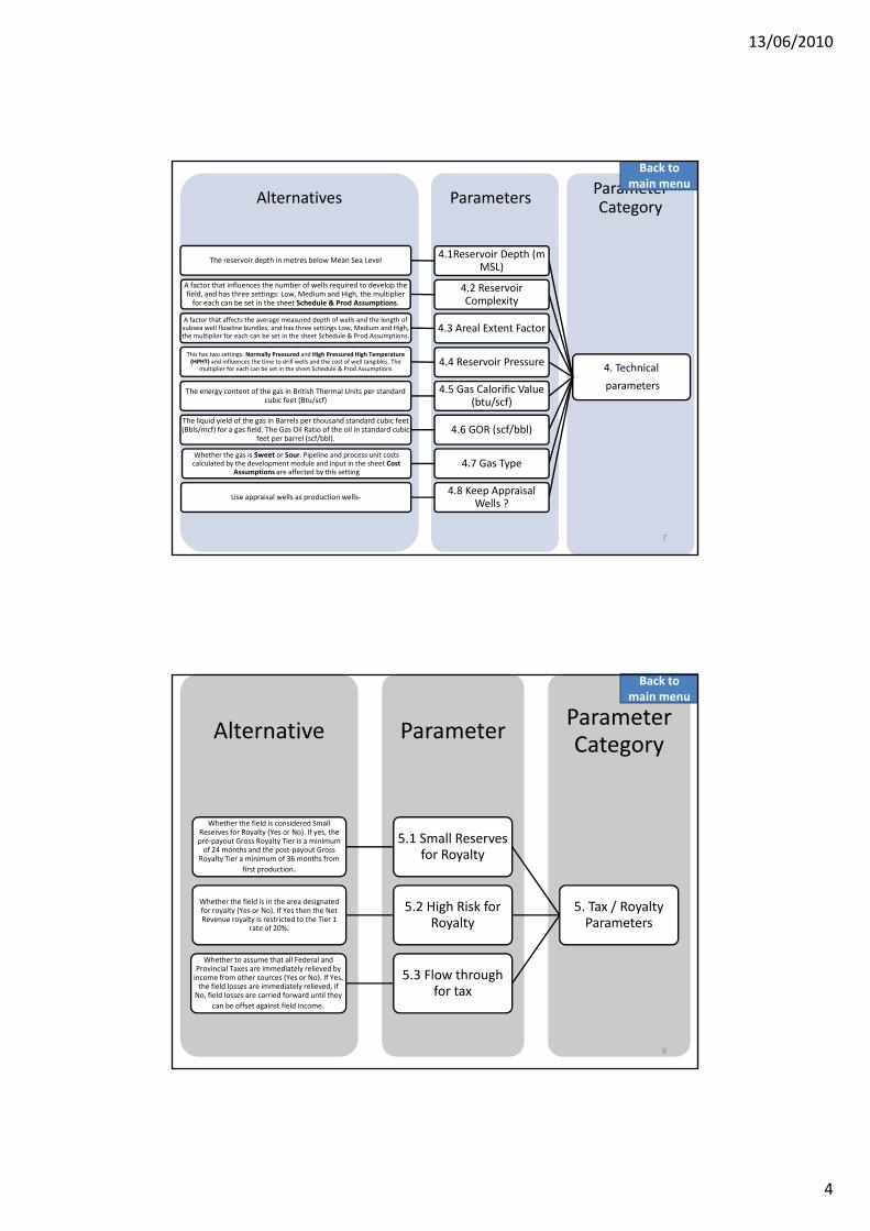
13/06/2010
4
ParameterCategory
4.1Reservoir Depth (m MSL)
The reservoir depth in metres below Mean Sea Level
4.2 ReservoirA factor that influences the number of wells required to develop the fi ld d h th tti L M di d Hi h th lti li
ParametersAlternatives
Back tomain menu
4. Technical
parameters
Complexityfield, and has three settings: Low, Medium and High, the multiplier for each can be set in the sheet Schedule & Prod Assumptions.
4.3 Areal Extent Factor A factor that affects the average measured depth of wells and the length of subsea well flowline bundles, and has three settings Low, Medium and High, the multiplier for each can be set in the sheet Schedule & Prod Assumptions.
4.4 Reservoir PressureThis has two settings: Normally Pressured and High Pressured High Temperature (HPHT) and influences the time to drill wells and the cost of well tangibles. The
multiplier for each can be set in the sheet Schedule & Prod Assumptions
4.5 Gas Calorific Value(btu/scf)
The energy content of the gas in British Thermal Units per standard cubic feet (Btu/scf)
The liquid yield of the gas in Barrels per thousand standard cubic feet 4.6 GOR (scf/bbl)
q y g p(Bbls/mcf) for a gas field. The Gas Oil Ratio of the oil in standard cubic
feet per barrel (scf/bbl).
4.7 Gas TypeWhether the gas is Sweet or Sour. Pipeline and process unit costs calculated by the development module and input in the sheet Cost
Assumptions are affected by this setting
4.8 Keep AppraisalWells ?
Use appraisal wells as production wells‐
7
Alternative Parameter ParameterCategory
Back tomain menu
5. Tax / Royalty Parameters
5.1 Small Reserves for Royalty
Whether the field is considered Small Reserves for Royalty (Yes or No). If yes, the pre‐payout Gross Royalty Tier is a minimum of 24 months and the post‐payout Gross
Royalty Tier a minimum of 36 months from first production.
5.2 High Risk forRoyalty
Whether the field is in the area designated for royalty (Yes or No). If Yes then the Net Revenue royalty is restricted to the Tier 1
rate of 20%.
5.3 Flow throughfor tax
Whether to assume that all Federal and Provincial Taxes are immediately relieved by income from other sources (Yes or No). If Yes, the field losses are immediately relieved, if No, field losses are carried forward until they
can be offset against field income.
8
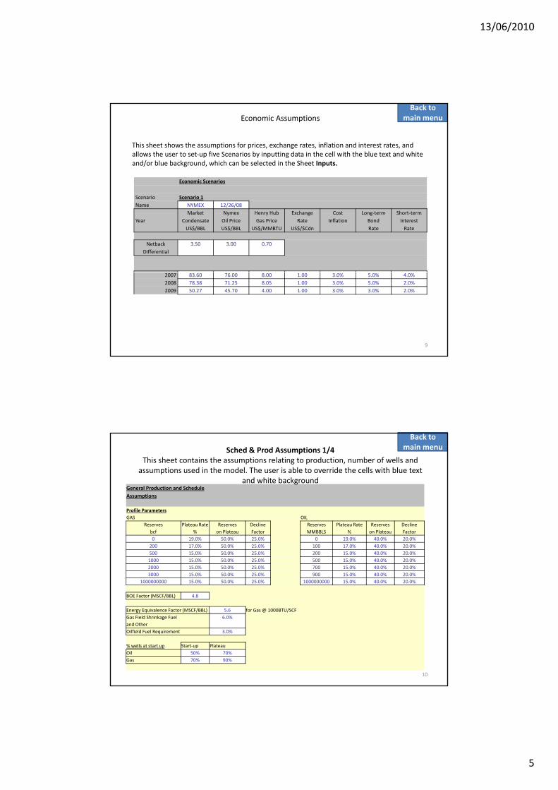
13/06/2010
5
Economic Scenarios
Economic Assumptions
This sheet shows the assumptions for prices, exchange rates, inflation and interest rates, and allows the user to set‐up five Scenarios by inputting data in the cell with the blue text and white and/or blue background, which can be selected in the Sheet Inputs.
Back tomain menu
Scenario Scenario 1Name NYMEX 12/26/08
Market Nymex Henry Hub Exchange Cost Long‐term Short‐termYear Condensate Oil Price Gas Price Rate Inflation Bond Interest
US$/BBL US$/BBL US$/MMBTU US$/$Cdn Rate Rate
Netback Differential
3.50 3.00 0.70
9
2007 83.60 76.00 8.00 1.00 3.0% 5.0% 4.0%2008 78.38 71.25 8.05 1.00 3.0% 5.0% 2.0%2009 50.27 45.70 4.00 1.00 3.0% 3.0% 2.0%
General Production and Schedule Assumptions
Profile ParametersGAS OIL
Sched & Prod Assumptions 1/4 This sheet contains the assumptions relating to production, number of wells and
assumptions used in the model. The user is able to override the cells with blue text and white background
Back tomain menu
GAS OILReserves Plateau Rate Reserves Decline Reserves Plateau Rate Reserves Decline
bcf % on Plateau Factor MMBBLS % on Plateau Factor0 19.0% 50.0% 25.0% 0 19.0% 40.0% 20.0%
200 17.0% 50.0% 25.0% 100 17.0% 40.0% 20.0%500 15.0% 50.0% 25.0% 200 15.0% 40.0% 20.0%1000 15.0% 50.0% 25.0% 500 15.0% 40.0% 20.0%2000 15.0% 50.0% 25.0% 700 15.0% 40.0% 20.0%3000 15.0% 50.0% 25.0% 900 15.0% 40.0% 20.0%
1000000000 15.0% 50.0% 25.0% 1000000000 15.0% 40.0% 20.0%
BOE Factor (MSCF/BBL) 4.8
10
Energy Equivalence Factor (MSCF/BBL) 5.6 for Gas @ 1000BTU/SCFGas Field Shrinkage Fuel and Other
6.0%
Oilfield Fuel Requirement 3.0%
% wells at start up Start‐up PlateauOil 50% 70%Gas 70% 90%
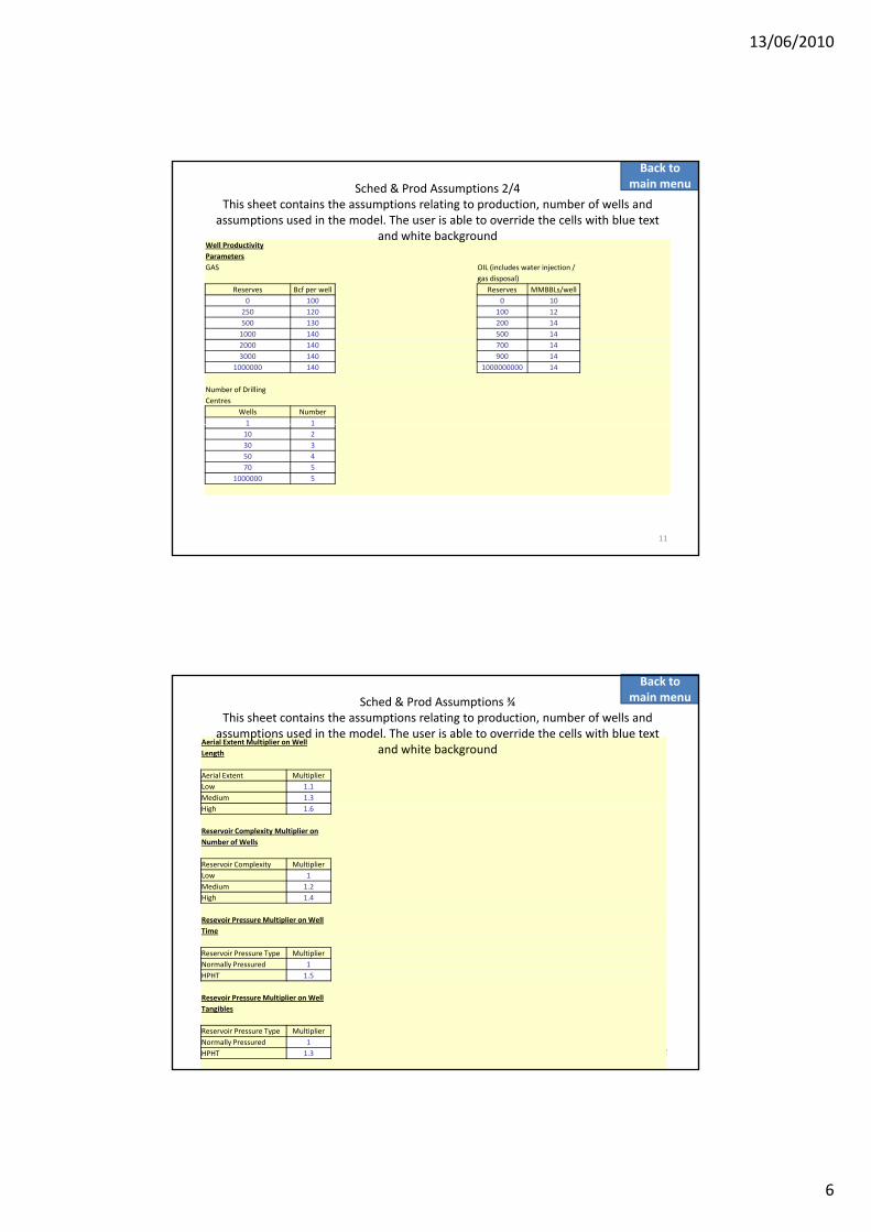
13/06/2010
6
Well ProductivityParametersGAS OIL (includes water injection /
gas disposal)Reserves Bcf per well Reserves MMBBLs/well
Sched & Prod Assumptions 2/4This sheet contains the assumptions relating to production, number of wells and
assumptions used in the model. The user is able to override the cells with blue text and white background
Back tomain menu
p /0 100 0 10
250 120 100 12500 130 200 141000 140 500 142000 140 700 143000 140 900 14
1000000 140 1000000000 14
Number of Drilling Centres
Wells Number1 1
11
1 110 230 350 470 5
1000000 5
Aerial Extent Multiplier on Well Length
Aerial Extent MultiplierLow 1.1Medium 1.3Hi h 1 6
Sched & Prod Assumptions ¾This sheet contains the assumptions relating to production, number of wells and
assumptions used in the model. The user is able to override the cells with blue text and white background
Back tomain menu
High 1.6
Reservoir Complexity Multiplier on Number of Wells
Reservoir Complexity MultiplierLow 1Medium 1.2High 1.4
Resevoir Pressure Multiplier on Well Time
12
Reservoir Pressure Type MultiplierNormally Pressured 1HPHT 1.5
Resevoir Pressure Multiplier on Well Tangibles
Reservoir Pressure Type MultiplierNormally Pressured 1HPHT 1.3
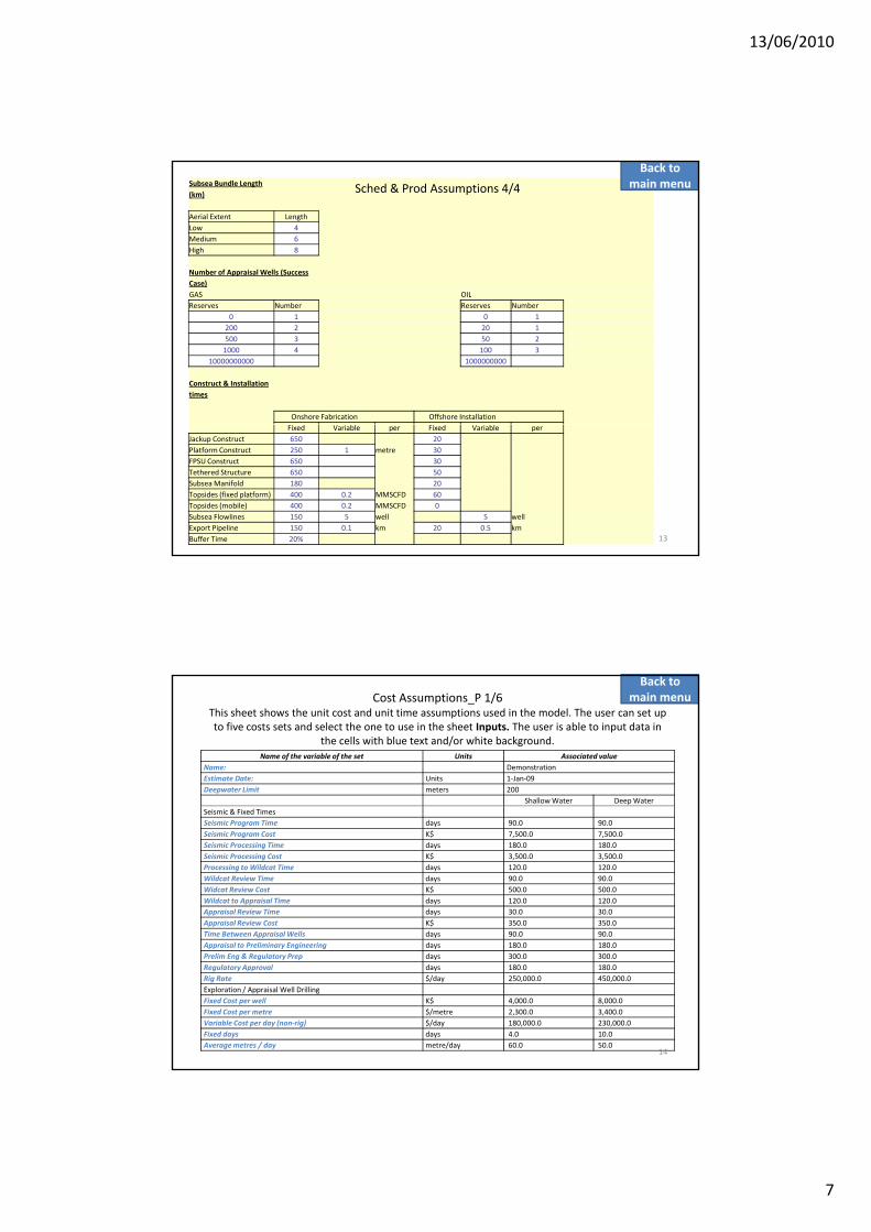
13/06/2010
7
Subsea Bundle Length(km)
Aerial Extent LengthLow 4Medium 6High 8
Number of Appraisal Wells (Success Case)GAS OIL
Sched & Prod Assumptions 4/4
Back tomain menu
GAS OILReserves Number Reserves Number
0 1 0 1200 2 20 1500 3 50 21000 4 100 3
10000000000 1000000000
Construct & Installation times
Onshore Fabrication Offshore Installation
13
Fixed Variable per Fixed Variable perJackup Construct 650 20Platform Construct 250 1 metre 30FPSU Construct 650 30Tethered Structure 650 50SubseaManifold 180 20Topsides (fixed platform) 400 0.2 MMSCFD 60Topsides (mobile) 400 0.2 MMSCFD 0Subsea Flowlines 150 5 well 5 wellExport Pipeline 150 0.1 km 20 0.5 kmBuffer Time 20%
Name of the variable of the set Units Associated valueName: DemonstrationEstimate Date: Units 1‐Jan‐09Deepwater Limit meters 200
Shallow Water Deep Water
Cost Assumptions_P 1/6This sheet shows the unit cost and unit time assumptions used in the model. The user can set up to five costs sets and select the one to use in the sheet Inputs. The user is able to input data in
the cells with blue text and/or white background.
Back tomain menu
Seismic & Fixed TimesSeismic Program Time days 90.0 90.0 Seismic Program Cost K$ 7,500.0 7,500.0 Seismic Processing Time days 180.0 180.0 Seismic Processing Cost K$ 3,500.0 3,500.0 Processing to Wildcat Time days 120.0 120.0 Wildcat Review Time days 90.0 90.0 Widcat Review Cost K$ 500.0 500.0 Wildcat to Appraisal Time days 120.0 120.0 Appraisal Review Time days 30.0 30.0 Appraisal Review Cost K$ 350.0 350.0 Time Between Appraisal Wells days 90.0 90.0 Appraisal to Preliminary Engineering days 180.0 180.0 Prelim Eng & Regulatory Prep days 300.0 300.0 Regulatory Approval days 180.0 180.0 Rig Rate $/day 250,000.0 450,000.0 Exploration / Appraisal Well DrillingFixed Cost per well K$ 4,000.0 8,000.0 Fixed Cost per metre $/metre 2,300.0 3,400.0 Variable Cost per day (non‐rig) $/day 180,000.0 230,000.0 Fixed days days 4.0 10.0 Average metres / day metre/day 60.0 50.0
14
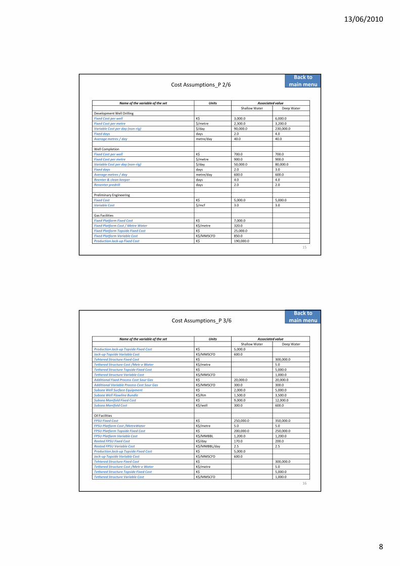
13/06/2010
8
Name of the variable of the set Units Associated valueShallow Water Deep Water
Development Well DrillingFixed Cost per well K$ 3,000.0 6,000.0 Fixed Cost per metre $/metre 2,300.0 3,200.0 Variable Cost per day (non‐rig) $/day 90,000.0 230,000.0 Fixed days days 2.0 4.0
Cost Assumptions_P 2/6Back to
main menu
Fixed days days 2.0 4.0 Average metres / day metre/day 40.0 40.0
Well CompletionFixed Cost per well K$ 700.0 700.0 Fixed Cost per metre $/metre 900.0 900.0 Variable Cost per day (non‐rig) $/day 50,000.0 80,000.0 Fixed days days 2.0 3.0 Average metres / day metre/day 600.0 600.0 Reenter & clean keeper days 4.0 4.0 Renenter predrill days 2.0 2.0
Preliminary EngineeringPreliminary EngineeringFixed Cost K$ 5,000.0 5,000.0 Variable Cost $/mcf 3.0 3.0
Gas FacilitiesFixed Platform Fixed Cost K$ 7,000.0 Fixed Platform Cost / Metre Water K$/metre 320.0 Fixed Platform Topside Fixed Cost K$ 25,000.0 Fixed Platform Variable Cost K$/MMSCFD 850.0 Production Jack‐up Fixed Cost K$ 190,000.0
15
Name of the variable of the set Units Associated valueShallow Water Deep Water
Production Jack‐up Topside Fixed Cost K$ 5,000.0 Jack‐up Topside Variable Cost K$/MMSCFD 600.0 Tehtered Structure Fixed Cost K$ 300,000.0 Tethered Structure Cost /Metr e Water K$/metre 5.0 Tethered Structure Topside Fixed Cost K$ 5,000.0
Cost Assumptions_P 3/6Back to
main menu
Tethered Structure Topside Fixed Cost K$ 5,000.0 Tethered Structure Variable Cost K$/MMSCFD 1,000.0 Additional Fixed Process Cost Sour Gas K$ 20,000.0 20,000.0 Additional Variable Process Cost Sour Gas K$/MMSCFD 300.0 300.0 Subsea Well Surface Equipment K$ 2,000.0 5,000.0 Subsea Well Flowline Bundle K$/Km 1,500.0 3,500.0 Subsea Manifold Fixed Cost K$ 9,000.0 12,000.0 Subsea Manifold Cost K$/well 300.0 600.0
Oil FacilitiesFPSU Fixed Cost K$ 250,000.0 350,000.0 FPSU Platform Cost /MetreWater K$/metre 5.0 5.0 FPSU Platform Topside Fixed Cost K$ 200 000 0 250 000 0FPSU Platform Topside Fixed Cost K$ 200,000.0 250,000.0 FPSU Platform Variable Cost K$/MMBBL 1,200.0 1,200.0 Rented FPSU Fixed Cost K$/day 170.0 200.0 Rented FPSU Variable Cost K$/MMBBL/day 2.5 2.5 Production Jack‐up Topside Fixed Cost K$ 5,000.0 Jack‐up Topside Variable Cost K$/MMSCFD 600.0 Tehtered Structure Fixed Cost K$ 300,000.0 Tethered Structure Cost /Metr e Water K$/metre 5.0 Tethered Structure Topside Fixed Cost K$ 5,000.0 Tethered Structure Variable Cost K$/MMSCFD 1,000.0
16
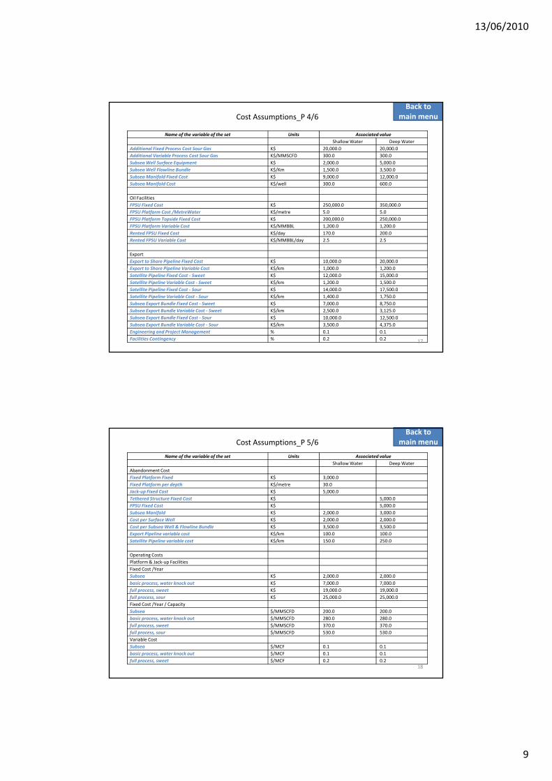
13/06/2010
9
Name of the variable of the set Units Associated valueShallow Water Deep Water
Additional Fixed Process Cost Sour Gas K$ 20,000.0 20,000.0 Additional Variable Process Cost Sour Gas K$/MMSCFD 300.0 300.0 Subsea Well Surface Equipment K$ 2,000.0 5,000.0 Subsea Well Flowline Bundle K$/Km 1,500.0 3,500.0 Subsea Manifold Fixed Cost K$ 9,000.0 12,000.0 Subsea Manifold Cost K$/well 300.0 600.0
Cost Assumptions_P 4/6Back to
main menu
f $/
Oil FacilitiesFPSU Fixed Cost K$ 250,000.0 350,000.0 FPSU Platform Cost /MetreWater K$/metre 5.0 5.0 FPSU Platform Topside Fixed Cost K$ 200,000.0 250,000.0 FPSU Platform Variable Cost K$/MMBBL 1,200.0 1,200.0 Rented FPSU Fixed Cost K$/day 170.0 200.0 Rented FPSU Variable Cost K$/MMBBL/day 2.5 2.5
ExportExport to Shore Pipeline Fixed Cost K$ 10,000.0 20,000.0 Export to Shore Pipeline Variable Cost K$/km 1 000 0 1 200 0Export to Shore Pipeline Variable Cost K$/km 1,000.0 1,200.0 Satellite Pipeline Fixed Cost ‐ Sweet K$ 12,000.0 15,000.0 Satellite Pipeline Variable Cost ‐ Sweet K$/km 1,200.0 1,500.0 Satellite Pipeline Fixed Cost ‐ Sour K$ 14,000.0 17,500.0 Satellite Pipeline Variable Cost ‐ Sour K$/km 1,400.0 1,750.0 Subsea Export Bundle Fixed Cost ‐ Sweet K$ 7,000.0 8,750.0 Subsea Export Bundle Variable Cost ‐ Sweet K$/km 2,500.0 3,125.0 Subsea Export Bundle Fixed Cost ‐ Sour K$ 10,000.0 12,500.0 Subsea Export Bundle Variable Cost ‐ Sour K$/km 3,500.0 4,375.0 Engineering and Project Management % 0.1 0.1 Facilities Contingency % 0.2 0.2 17
Name of the variable of the set Units Associated valueShallow Water Deep Water
Abandonment CostFixed Platform Fixed K$ 3,000.0 Fixed Platform per depth K$/metre 30.0 Jack‐up Fixed Cost K$ 5,000.0 Tethered Structure Fixed Cost K$ 5,000.0 FPSU Fixed Cost K$ 5,000.0 S b M if ld K$ 2 000 0 3 000 0
Cost Assumptions_P 5/6Back to
main menu
Subsea Manifold K$ 2,000.0 3,000.0 Cost per Surface Well K$ 2,000.0 2,000.0 Cost per Subsea Well & Flowline Bundle K$ 3,500.0 3,500.0 Export Pipeline variable cost K$/km 100.0 100.0 Satellite Pipeline variable cost K$/km 150.0 250.0
Operating CostsPlatform & Jack‐up FacilitiesFixed Cost /Year Subsea K$ 2,000.0 2,000.0 basic process, water knock out K$ 7,000.0 7,000.0 full process, sweet K$ 19,000.0 19,000.0 full process, sour K$ 25,000.0 25,000.0 Fixed Cost /Year / CapacitySubsea $/MMSCFD 200.0 200.0 basic process, water knock out $/MMSCFD 280.0 280.0 full process, sweet $/MMSCFD 370.0 370.0 full process, sour $/MMSCFD 530.0 530.0 Variable CostSubsea $/MCF 0.1 0.1 basic process, water knock out $/MCF 0.1 0.1 full process, sweet $/MCF 0.2 0.2
18
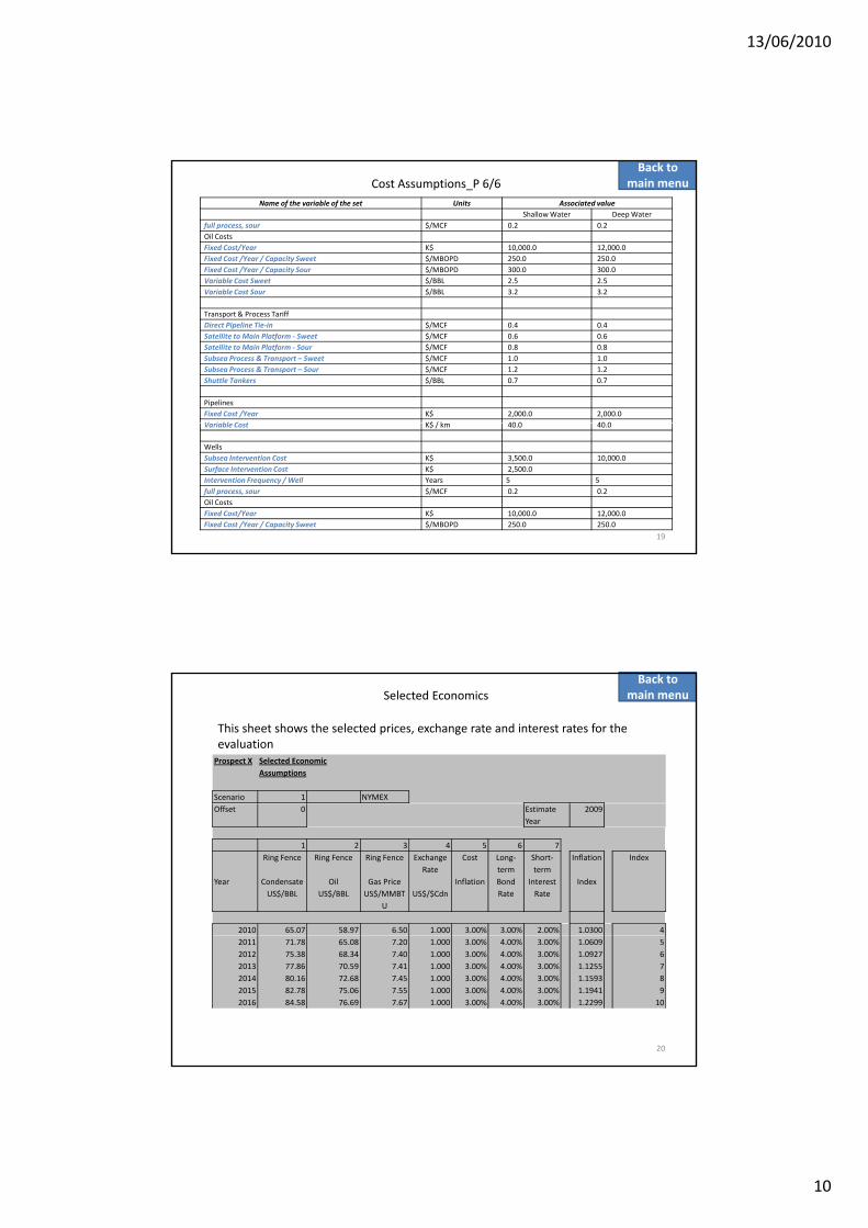
13/06/2010
10
Name of the variable of the set Units Associated valueShallow Water Deep Water
full process, sour $/MCF 0.2 0.2 Oil CostsFixed Cost/Year K$ 10,000.0 12,000.0 Fixed Cost /Year / Capacity Sweet $/MBOPD 250.0 250.0 Fixed Cost /Year / Capacity Sour $/MBOPD 300.0 300.0 Variable Cost Sweet $/BBL 2.5 2.5 Variable Cost Sour $/BBL 3 2 3 2
Cost Assumptions_P 6/6Back to
main menu
Variable Cost Sour $/BBL 3.2 3.2
Transport & Process TariffDirect Pipeline Tie‐in $/MCF 0.4 0.4 Satellite to Main Platform ‐ Sweet $/MCF 0.6 0.6 Satellite to Main Platform ‐ Sour $/MCF 0.8 0.8 Subsea Process & Transport – Sweet $/MCF 1.0 1.0 Subsea Process & Transport – Sour $/MCF 1.2 1.2 Shuttle Tankers $/BBL 0.7 0.7
PipelinesFixed Cost /Year K$ 2,000.0 2,000.0 V i bl C t K$ / k 40 0 40 0Variable Cost K$ / km 40.0 40.0
WellsSubsea Intervention Cost K$ 3,500.0 10,000.0 Surface Intervention Cost K$ 2,500.0 Intervention Frequency / Well Years 5 5full process, sour $/MCF 0.2 0.2 Oil CostsFixed Cost/Year K$ 10,000.0 12,000.0 Fixed Cost /Year / Capacity Sweet $/MBOPD 250.0 250.0
19
Prospect X Selected Economic Assumptions
Scenario 1 NYMEX
Selected Economics
This sheet shows the selected prices, exchange rate and interest rates for the evaluation
Back tomain menu
Offset 0 Estimate Year
2009
1 2 3 4 5 6 7Ring Fence Ring Fence Ring Fence Exchange
RateCost Long‐
termShort‐term
Inflation Index
Year Condensate Oil Gas Price Inflation Bond Interest IndexUS$/BBL US$/BBL US$/MMBT
UUS$/$Cdn Rate Rate
2010 65.07 58.97 6.50 1.000 3.00% 3.00% 2.00% 1.0300 4
20
2011 71.78 65.08 7.20 1.000 3.00% 4.00% 3.00% 1.0609 52012 75.38 68.34 7.40 1.000 3.00% 4.00% 3.00% 1.0927 62013 77.86 70.59 7.41 1.000 3.00% 4.00% 3.00% 1.1255 72014 80.16 72.68 7.45 1.000 3.00% 4.00% 3.00% 1.1593 82015 82.78 75.06 7.55 1.000 3.00% 4.00% 3.00% 1.1941 92016 84.58 76.69 7.67 1.000 3.00% 4.00% 3.00% 1.2299 10
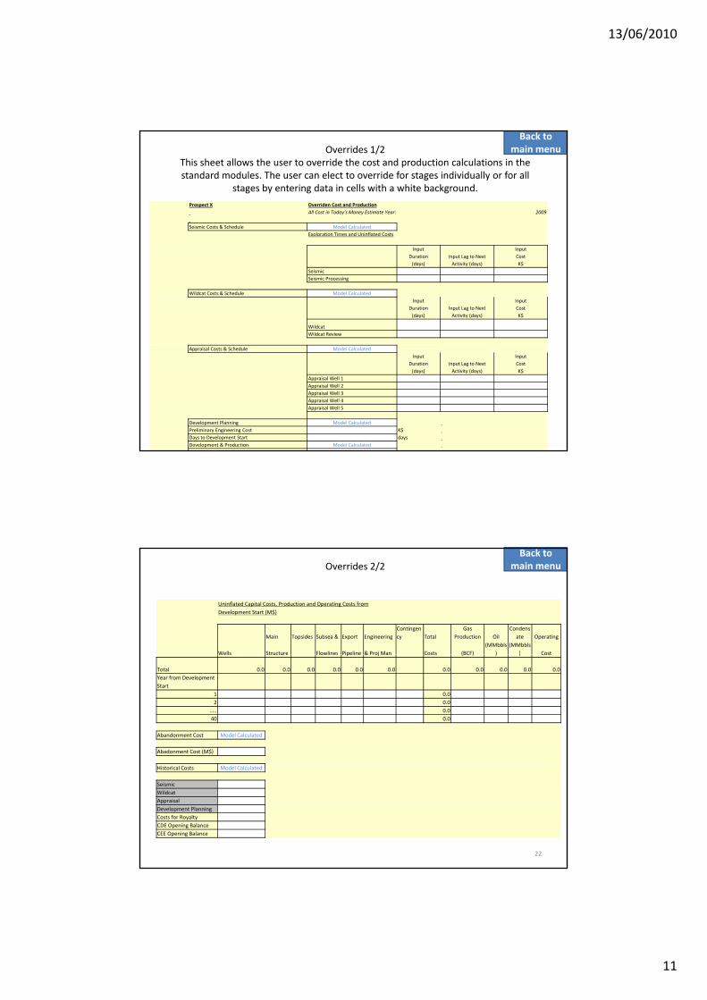
13/06/2010
11
Prospect X Overriden Cost and ProductionAll Cost in Today's Money Estimate Year: 2009
Seismic Costs & Schedule Model CalculatedExoloration Times and Uninflated Costs
Overrides 1/2This sheet allows the user to override the cost and production calculations in the standard modules. The user can elect to override for stages individually or for all
stages by entering data in cells with a white background.
Back tomain menu
InputInput Lag to Next Activity (days)
Input Duration Cost(days) K$
SeismicSeismic Processing
Wildcat Costs & Schedule Model CalculatedInput
Input Lag to Next Activity (days)
Input Duration Cost(days) K$
WildcatWildcat Review
21
Appraisal Costs & Schedule Model CalculatedInput
Input Lag to Next Activity (days)
Input Duration Cost(days) K$
Appraisal Well 1Appraisal Well 2Appraisal Well 3Appraisal Well 4Appraisal Well 5
Development Planning Model CalculatedPreliminary Engineering Cost K$Days to Development Start daysDevelopment & Production Model CalculatedOperating Costs Model Calculated
Uninflated Capital Costs, Production and Operating Costs from Development Start (M$)
Main Topsides Subsea & Export EngineeringContingency Total
Gas Production Oil
Condensate Operating
Wells Structure Flowlines Pipeline & Proj Man Costs (BCF)(MMbbls
)(MMbbls
) Cost
Overrides 2/2Back to
main menu
Wells Structure Flowlines Pipeline & Proj Man Costs (BCF) ) ) Cost
Total 0.0 0.0 0.0 0.0 0.0 0.0 0.0 0.0 0.0 0.0 0.0Year from Development Start
1 0.02 0.0
….. 0.040 0.0
Abandonment Cost Model Calculated
Abadonment Cost (M$)
22
Historical Costs Model Calculated
SeismicWildcatAppraisalDevelopment PlanningCosts for RoyaltyCDE Opening BalanceCEE Opening Balance
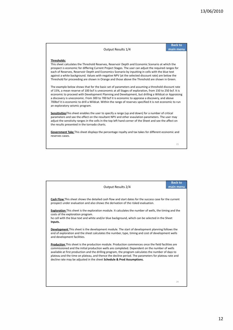
13/06/2010
12
Thresholds:This sheet calculates the Threshold Reserves, Reservoir Depth and Economic Scenario at which the prospect is economic for differing Current Project Stages. The user can adjust the required ranges for each of Reserves, Reservoir Depth and Economics Scenario by inputting in cells with the blue text against a white background. Values with negative NPV (at the selected discount rate) are below the Th h ld f di h i O d h b h Th h ld h i G
Output Results 1/4Back to
main menu
Threshold for proceeding are shown in Orange and those above the Threshold are shown in Green.
The example below shows that for the basic set of parameters and assuming a threshold discount rate of 15%, a mean reserve of 100 bcf is uneconomic at all Stages of exploration, from 150 to 250 bcf. It is economic to proceed with Development Planning and Development, but drilling a Wildcat or Appraising a discovery is uneconomic. From 300 to 700 bcf it is economic to appraise a discovery, and above 700bcf it is economic to drill a Wildcat. Within the range of reserves specified it is not economic to run an exploratory seismic program.
SensitivitiesThis sheet enables the user to specify a range (up and down) for a number of critical
23
SensitivitiesThis sheet enables the user to specify a range (up and down) for a number of critical parameters and see the effect on the resultant NPV and other evaulation parameters. The user may adjust the senstivity ranges in the cells in the top left hand corner of the Sheet and see the affect on the results presented in the tornado charts.
Government Take This sheet displays the percentage royalty and tax takes for different economic and reserves cases.
Cash Flow This sheet shows the detailed cash flow and start dates for the success case for the current prospect under evaluation and also shows the derivation of the risked evaluation.
Exploration This sheet is the exploration module. It calculates the number of wells, the timing and the costs of the exploration program.
Output Results 2/4Back to
main menu
he cell with the blue text and white and/or blue background, which can be selected in the Sheet Inputs.
Development This sheet is the development module. The start of development planning follows the end of exploration and the sheet calculates the number, type, timing and cost of development wells and development facilities.
Production This sheet is the production module. Production commences once the field facilities are commissioned and the initial production wells are completed. Dependent on the number of wells
il bl t fi t d ti d th d illi th l l t th b f d t
24
available at first production and the drilling program, the program calculates the number of days to plateau and the time on plateau, and thence the decline period. The parameters for plateau rate and decline rate may be adjusted in the sheet Schedule & Prod Assumptions.
13/06/2010
13
Revenue This sheet calculates the gas and liquids revenue
Operations This sheet is the operations module and calculates the operating costs for the field life
Abandonment This sheet calculates the economic limit for the field and the abandonment cost. Production and operating costs are terminated at abandonment.
Output Results 3/4Back to
main menu
Royalty This sheet calculates the royalty for the success case. For prospects commencing after the initial seismic phase, historical costs are estimated, but can be overridden in Cell C101 of sheet Overrides. The royalty calculation estimates the month at which the change over between each royalty tier is made.
Federal Tax This sheet calculates the federal income tax payable for the field. As with royalty, the historical costs are estimated by the model but can be overridden by the user in cells C102 and C103 of sheet Overrides.
25
Provincial Tax This sheet calculates the provincial income tax payable for the field. As with royalty, the historical costs are estimated by the model but can be overridden by the user in cells C102 and C103 of sheet Overrides.
Success Cash Flow This sheet shows the success case cash flow for the prospect
Risked Cash Flow This sheet shows the risked cash flow for the field
Output Results 4/4Back to
main menu
26
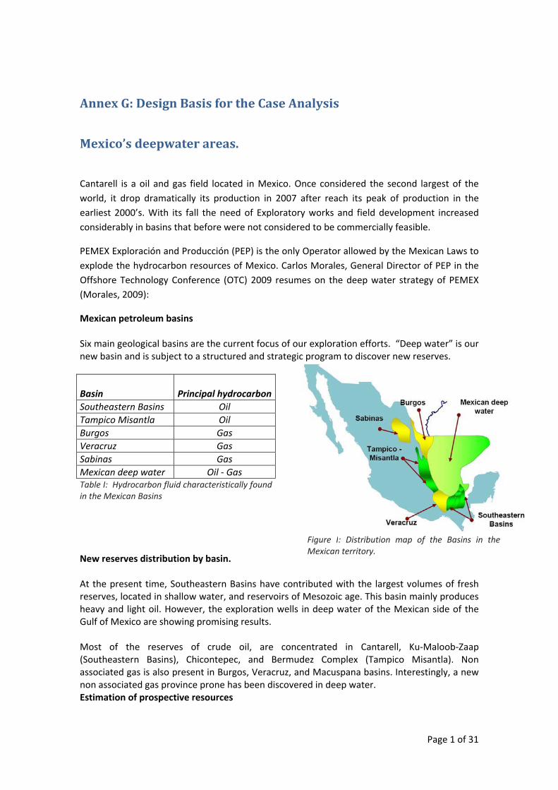
Page 1 of 31
Annex G: Design Basis for the Case Analysis
Mexico’s deepwater areas.
Cantarell is a oil and gas field located in Mexico. Once considered the second largest of the world, it drop dramatically its production in 2007 after reach its peak of production in the earliest 2000’s. With its fall the need of Exploratory works and field development increased considerably in basins that before were not considered to be commercially feasible.
PEMEX Exploración and Producción (PEP) is the only Operator allowed by the Mexican Laws to explode the hydrocarbon resources of Mexico. Carlos Morales, General Director of PEP in the Offshore Technology Conference (OTC) 2009 resumes on the deep water strategy of PEMEX (Morales, 2009):
Mexican petroleum basins Six main geological basins are the current focus of our exploration efforts. “Deep water” is our new basin and is subject to a structured and strategic program to discover new reserves.
New reserves distribution by basin. At the present time, Southeastern Basins have contributed with the largest volumes of fresh reserves, located in shallow water, and reservoirs of Mesozoic age. This basin mainly produces heavy and light oil. However, the exploration wells in deep water of the Mexican side of the Gulf of Mexico are showing promising results. Most of the reserves of crude oil, are concentrated in Cantarell, Ku‐Maloob‐Zaap (Southeastern Basins), Chicontepec, and Bermudez Complex (Tampico Misantla). Non associated gas is also present in Burgos, Veracruz, and Macuspana basins. Interestingly, a new non associated gas province prone has been discovered in deep water. Estimation of prospective resources
Basin
Principal hydrocarbon
Southeastern Basins Oil Tampico Misantla Oil Burgos Gas Veracruz Gas Sabinas Gas Mexican deep water Oil ‐ Gas Table I: Hydrocarbon fluid characteristically found in the Mexican Basins
Figure I: Distribution map of the Basins in the Mexican territory.
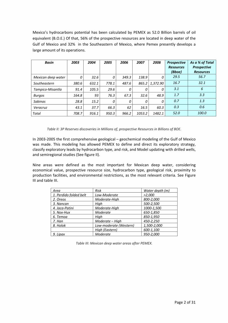
Page 2 of 31
Mexico’s hydrocarbons potential has been calculated by PEMEX as 52.0 Billion barrels of oil equivalent (B.O.E.) Of that, 56% of the prospective resources are located in deep water of the Gulf of Mexico and 32% in the Southeastern of Mexico, where Pemex presently develops a large amount of its operations.
Table II: 3P Reserves discoveries in Millions of, prospective Resources in Billions of BOE. In 2003‐2005 the first comprehensive geological – geochemical modeling of the Gulf of Mexico was made. This modeling has allowed PEMEX to define and direct its exploratory strategy, classify exploratory leads by hydrocarbon type, and risk, and Model updating with drilled wells, and semiregional studies (See figure II). Nine areas were defined as the most important for Mexican deep water, considering economical value, prospective resource size, hydrocarbon type, geological risk, proximity to production facilities, and environmental restrictions, as the most relevant criteria. See Figure III and table III.
Area Risk Water depth (m) 1. Perdido folded belt Low‐Moderate >2,0002. Oreos Moderate‐High 800‐2,0003. Nancan High 500‐2,5004. Jaca‐Patini Moderate‐High 1000‐1,500 5. Nox‐Hux Moderate 650‐1,8506. Temoa High 850‐1,9507. Han Moderate – High 450‐2,2508. Holok Low‐moderate (Western) 1,500‐2,000 High (Eastern) 600‐1,1009. Lipax Moderate 950‐2,000
Table III: Mexican deep water areas after PEMEX.
Basin 2003 2004 2005 2006 2007 2008 Prospective Resources (Bboe)
As a % of Total Prospective Resources
Mexican deep water 0 32.6 0 349.3 138.9 0 29.5 56.7
Southeastern 380.6 632.1 778.1 487.6 865.2 1,372.90 16.7 32.1
Tampico‐Misantla 91.4 105.5 29.6 0 0 0 3.1 6
Burgos 164.8 93 76.3 67.3 32.6 48.9 1.7 3.3
Sabinas 28.8 15.2 0 0 0 0 0.7 1.3
Veracruz 43.1 37.7 66.3 62 16.5 60.3 0.3 0.6
Total 708.7 916.1 950.3 966.2 1053.2 1482.1 52.0 100.0
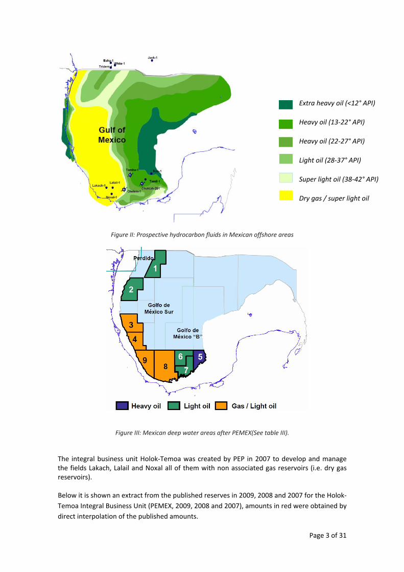
Page 3 of 31
Figure II: Prospective hydrocarbon fluids in Mexican offshore areas
Figure III: Mexican deep water areas after PEMEX(See table III).
The integral business unit Holok‐Temoa was created by PEP in 2007 to develop and manage the fields Lakach, Lalail and Noxal all of them with non associated gas reservoirs (i.e. dry gas reservoirs). Below it is shown an extract from the published reserves in 2009, 2008 and 2007 for the Holok‐Temoa Integral Business Unit (PEMEX, 2009, 2008 and 2007), amounts in red were obtained by direct interpolation of the published amounts.
• Extra heavy oil (<12° API) • • Heavy oil (13‐22° API) • • Heavy oil (22‐27° API) • • Light oil (28‐37° API) • • Super light oil (38‐42° API) • • Dry gas / super light oil
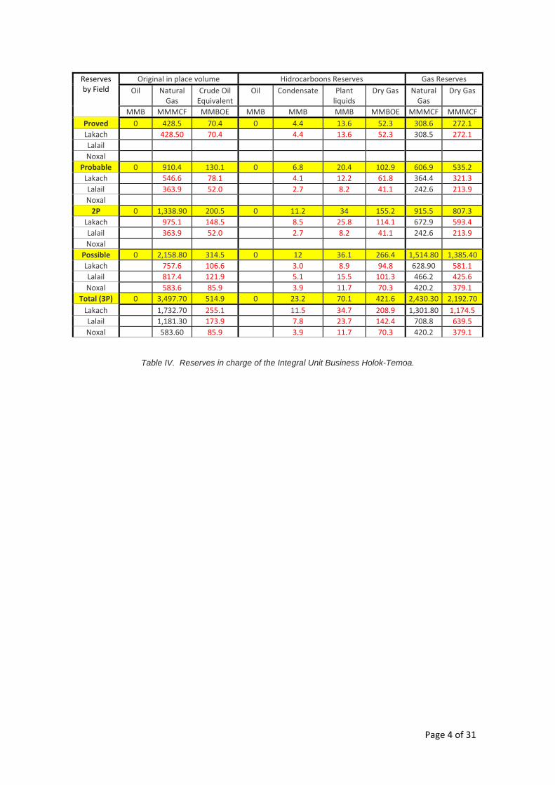
Page 4 of 31
Reserves by Field
Original in place volume Hidrocarboons Reserves Gas Reserves Oil Natural
Gas Crude Oil Equivalent
Oil Condensate Plant liquids
Dry Gas Natural Gas
Dry Gas
MMB MMMCF MMBOE MMB MMB MMB MMBOE MMMCF MMMCF Proved 0 428.5 70.4 0 4.4 13.6 52.3 308.6 272.1 Lakach 428.50 70.4 4.4 13.6 52.3 308.5 272.1 Lalail Noxal
Probable 0 910.4 130.1 0 6.8 20.4 102.9 606.9 535.2 Lakach 546.6 78.1 4.1 12.2 61.8 364.4 321.3 Lalail 363.9 52.0 2.7 8.2 41.1 242.6 213.9 Noxal 2P 0 1,338.90 200.5 0 11.2 34 155.2 915.5 807.3
Lakach 975.1 148.5 8.5 25.8 114.1 672.9 593.4 Lalail 363.9 52.0 2.7 8.2 41.1 242.6 213.9 Noxal
Possible 0 2,158.80 314.5 0 12 36.1 266.4 1,514.80 1,385.40 Lakach 757.6 106.6 3.0 8.9 94.8 628.90 581.1 Lalail 817.4 121.9 5.1 15.5 101.3 466.2 425.6 Noxal 583.6 85.9 3.9 11.7 70.3 420.2 379.1
Total (3P) 0 3,497.70 514.9 0 23.2 70.1 421.6 2,430.30 2,192.70 Lakach 1,732.70 255.1 11.5 34.7 208.9 1,301.80 1,174.5 Lalail 1,181.30 173.9 7.8 23.7 142.4 708.8 639.5 Noxal 583.60 85.9 3.9 11.7 70.3 420.2 379.1
Table IV. Reserves in charge of the Integral Unit Business Holok-Temoa.
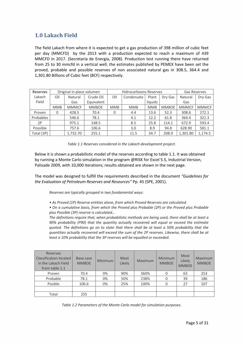
Page 5 of 31
1.0 Lakach Field The field Lakach from where it is expected to get a gas production of 398 million of cubic feet per day (MMCFD) by the 2013 with a production expected to reach a maximum of 439 MMCFD in 2017. (Secretaría de Energía, 2008). Production test running there have returned from 25 to 30 mmcfd in a vertical well, the estimates published by PEMEX have been set the proved, probable and possible reserves of non associated natural gas in 308.5, 364.4 and 1,301.80 Billions of Cubic feet (BCF) respectively.
Reserves Lakach Field
Original in place volumen Hidrocarboons Reserves Gas Reserves Oil Natural
Gas Crude Oil Equivalent
Oil Condensate Plant liquids
Dry Gas Natural Gas
Dry Gas
MMB MMMCF MMBOE MMB MMB MMB MMBOE MMMCF MMMCF Proven 0 428.5 70.4 0 4.4 13.6 52.3 308.6 272.1
Probables 546.6 78.1 4.1 12.2 61.8 364.4 321.32P 975.1 148.5 8.5 25.8 114.1 672.9 593.4
Possible 757.6 106.6 3.0 8.9 94.8 628.90 581.1Total (3P) 1,732.70 255.1 11.5 34.7 208.9 1,301.80 1,174.5
Table 1.1 Reserves considered in the Lakach development project.
Below it is shown a probabilistic model of the reserves according to table 1.1. It was obtained by running a Monte Carlo simulation in the program @RISK for Excel 5.5, Industrial Version, Palisade 2009, with 10,000 iterations; results obtained are shown in the next page. The model was designed to fulfill the requirements described in the document “Guidelines for the Evaluation of Petroleum Reserves and Resources” Pp. 45 (SPE, 2001).
Reserves are typically grouped in two fundamental ways: • As Proved (1P) Reserve entities alone, from which Proved Reserves are calculated. • On a cumulative basis, from which the Proved plus Probable (2P) or the Proved plus Probable plus Possible (3P) reserve is calculated… The definitions require that, when probabilistic methods are being used, there shall be at least a 90% probability (P90) that the quantity actually recovered will equal or exceed the estimate quoted. The definitions go on to state that there shall be at least a 50% probability that the quantities actually recovered will exceed the sum of the 2P reserves. Likewise, there shall be at least a 10% probability that the 3P reserves will be equalled or exceeded.
Reserves
Classification located in the Lakach Field from table 1.1
Base case MMBOE
MinimumMost Likely
Maximum Minimum MMBOE
Most Likely
MMBOE
MaximumMMBOE
Proven 70.4 0% 90% 360% 0 63 253Probable 78.1 0% 50% 238% 0 39 186Posible 106.6 0% 25% 100% 0 27 107
Total 255
Table 1.2 Parameters of the Monte Carlo model for simulation purposes.
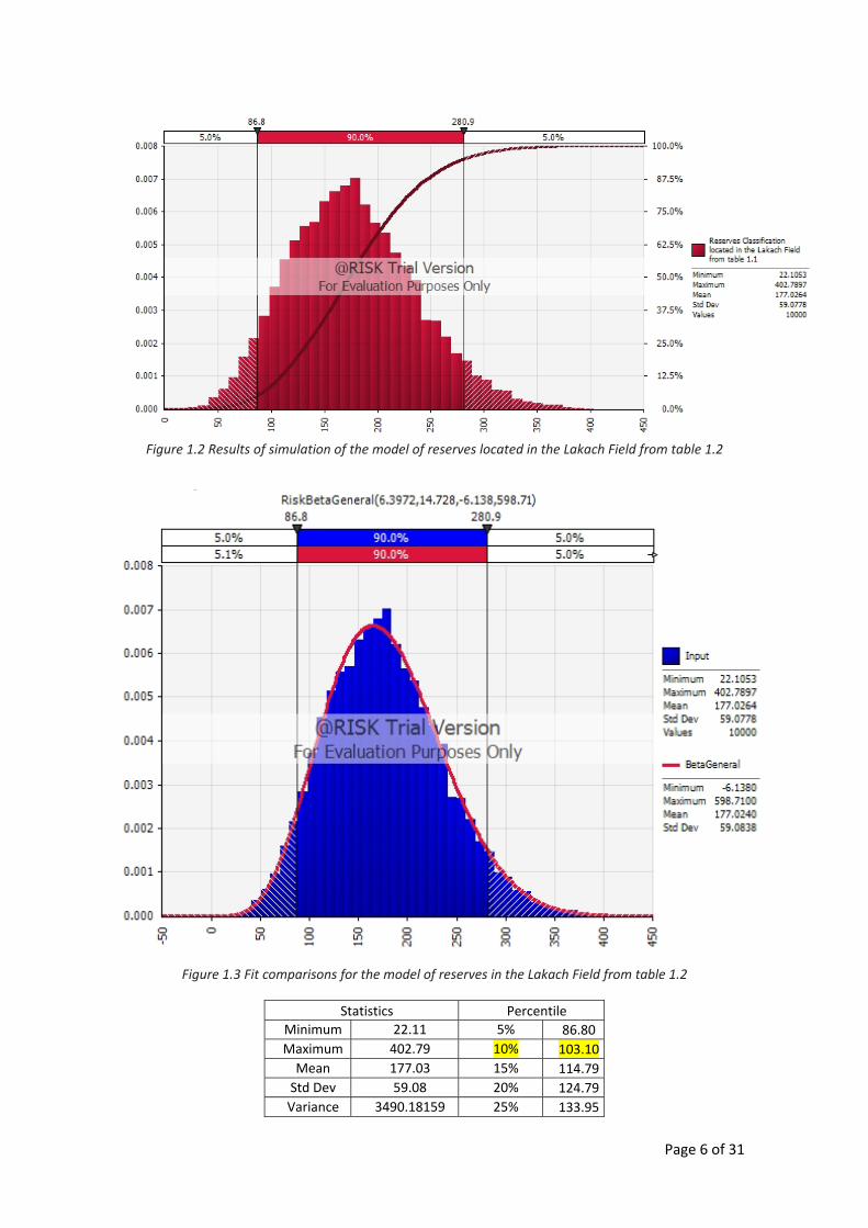
Page 6 of 31
Figure 1.2 Results of simulation of the model of reserves located in the Lakach Field from table 1.2
Figure 1.3 Fit comparisons for the model of reserves in the Lakach Field from table 1.2
Statistics Percentile Minimum 22.11 5% 86.80 Maximum 402.79 10% 103.10Mean 177.03 15% 114.79Std Dev 59.08 20% 124.79Variance 3490.18159 25% 133.95

Page 7 of 31
Skewness 0.351521499 30% 143.07Kurtosis 2.946435815 35% 151.05Median 173.62 40% 158.92Mode 181.54 45% 166.27Left X 86.80 50% 173.62Left P 5% 55% 180.95Right X 280.90 60% 188.51Right P 95% 65% 196.77Diff X 194.11 70% 205.98Diff P 90% 75% 215.45#Errors 0 80% 226.01Filter Min Off 85% 238.86Filter Max Off 90% 255.92#Filtered 0 95% 280.90
Table 1.3 Summary statistics from the simulation of the model of reserves in the Lakach Field from table 1.2 The Lakach development project has a total budget of 14,575.8 million Mexican pesos (approximately 1,100 Millions of USD) along 5 years from 2007 according to the information provided by the Ministry of Energy of Mexico in its 2nd. Inform of Results (SENER, 2008). The resources for this project are to be used in activities of delimitation of the reservoir and the offshore field development.
2.0 DESIGN BASIS
2.1 Reservoir characteristics The following information has been taken from the document Hydrocarbon Reserves of Mexico Evaluation as of January 1, 2007. Pp 36‐41 (Pemex, 2007).
Structural Geology In the tectonic structure, the Lakach field is an anticline to the south of the Lakach‐Labay alignment in a northwest‐southeast direction. The alignment is located at the southeastern end of the Mexican Cordilleras, Figure 4.2. (See figure 2.1 in this document) Stratigraphy The stratigraphic column cut by the Lakach‐1 well, which consists of rock the range from the Recent‐Pleistocene to the Lower Miocene, is made up an interbedding of clay horizons with limolites and lithic sandstones. The rocks that form the Lower Miocene age reservoirs mostly consist of lithic sandstone and limolites, and correspond to turbiditic fans and submarine channels in a slope environment. Seal The rock seal of the upper and lower part of both reservoirs largely consists of shales more than 30 meters thick and with broad lateral distribution. It is a combined type: structurally it is confined by an asymmetric anticline with its own closing at a reservoir level, whose dimensions are 10 kilometers long and 2 kilometers wide for reservoir
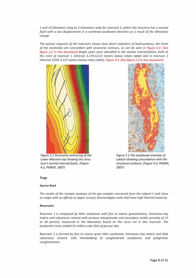
Page 8 of 31
1 and 13 kilometers long by 2 kilometers wide for reservoir 2, where the structure has a normal fault with a low displacement in a northeast‐southwest direction as a result of the lithostatic charge. The seismic response of the reservoirs shows clear direct indicators of hydrocarbons; the limits of the anomalies are concordant with structural contours, as can be seen in Figure 4.3. (See figure 2.2 in this document) Bright spots were identified in the seismic interpretation, both at the crest of reservoir 1 (interval 3,174‐3,212 meters below rotary table) and in reservoir 2 (interval 3,035‐3,127 meters below rotary table), Figure 4.4. (See figure 2.3 in this document)
Trap
Source Rock The results of the isotopic analyses of the gas samples recovered from the Lakach‐1 well show an origin with an affinity to Upper Jurassic Kimmeridgian rocks that have high thermal maturity. Reservoirs Reservoir 1 is composed by lithic sandstone with fine to coarse granulometry, limestone‐clay matrix and calcareous cement with primary intergranular and secondary moldic porosity of 15 to 28 percent, measured in the laboratory based on the cores cut in this reservoir. The production tests yielded 25 million cubic feet of gas per day. Reservoir 2 is formed by fine to coarse grain lithic sandstone, limestone‐clay matrix and little calcareous cement, with interbedding of conglomerate sandstones and poligmithic conglomerates.
Figure 2.1 Structural contouring of the Lower Miocene top showing the struc‐ture’s normal internal faults. (Figure 4.2, PEMEX, 2007)
Figure 2.2 The amplitude anomaly of Lakach showing concordance with the structural contours. (Figure 4.3, PEMEX, 2007)
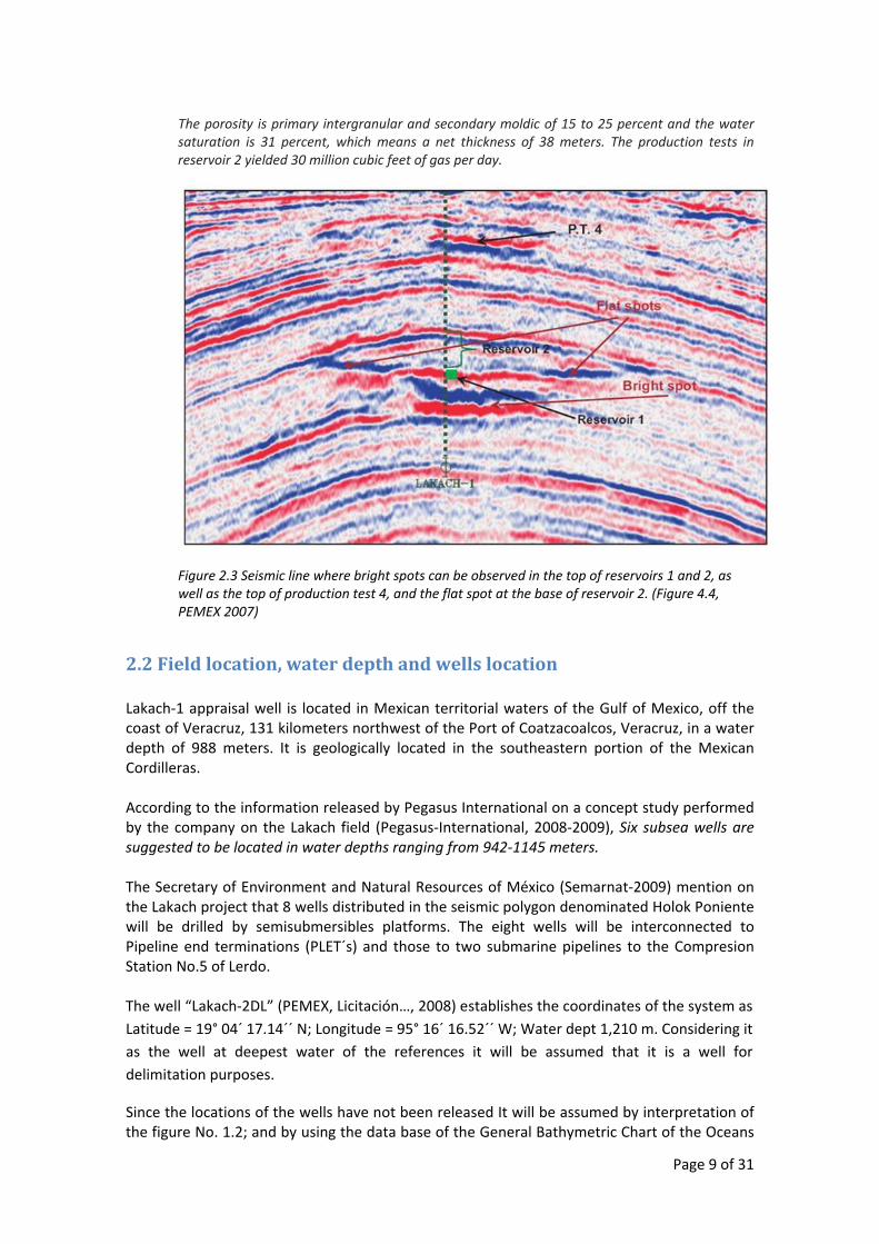
Page 9 of 31
The porosity is primary intergranular and secondary moldic of 15 to 25 percent and the water saturation is 31 percent, which means a net thickness of 38 meters. The production tests in reservoir 2 yielded 30 million cubic feet of gas per day.
Figure 2.3 Seismic line where bright spots can be observed in the top of reservoirs 1 and 2, as well as the top of production test 4, and the flat spot at the base of reservoir 2. (Figure 4.4, PEMEX 2007)
2.2 Field location, water depth and wells location Lakach‐1 appraisal well is located in Mexican territorial waters of the Gulf of Mexico, off the coast of Veracruz, 131 kilometers northwest of the Port of Coatzacoalcos, Veracruz, in a water depth of 988 meters. It is geologically located in the southeastern portion of the Mexican Cordilleras. According to the information released by Pegasus International on a concept study performed by the company on the Lakach field (Pegasus‐International, 2008‐2009), Six subsea wells are suggested to be located in water depths ranging from 942‐1145 meters. The Secretary of Environment and Natural Resources of México (Semarnat‐2009) mention on the Lakach project that 8 wells distributed in the seismic polygon denominated Holok Poniente will be drilled by semisubmersibles platforms. The eight wells will be interconnected to Pipeline end terminations (PLET´s) and those to two submarine pipelines to the Compresion Station No.5 of Lerdo. The well “Lakach‐2DL” (PEMEX, Licitación…, 2008) establishes the coordinates of the system as Latitude = 19° 04´ 17.14´´ N; Longitude = 95° 16´ 16.52´´ W; Water dept 1,210 m. Considering it as the well at deepest water of the references it will be assumed that it is a well for delimitation purposes.
Since the locations of the wells have not been released It will be assumed by interpretation of the figure No. 1.2; and by using the data base of the General Bathymetric Chart of the Oceans
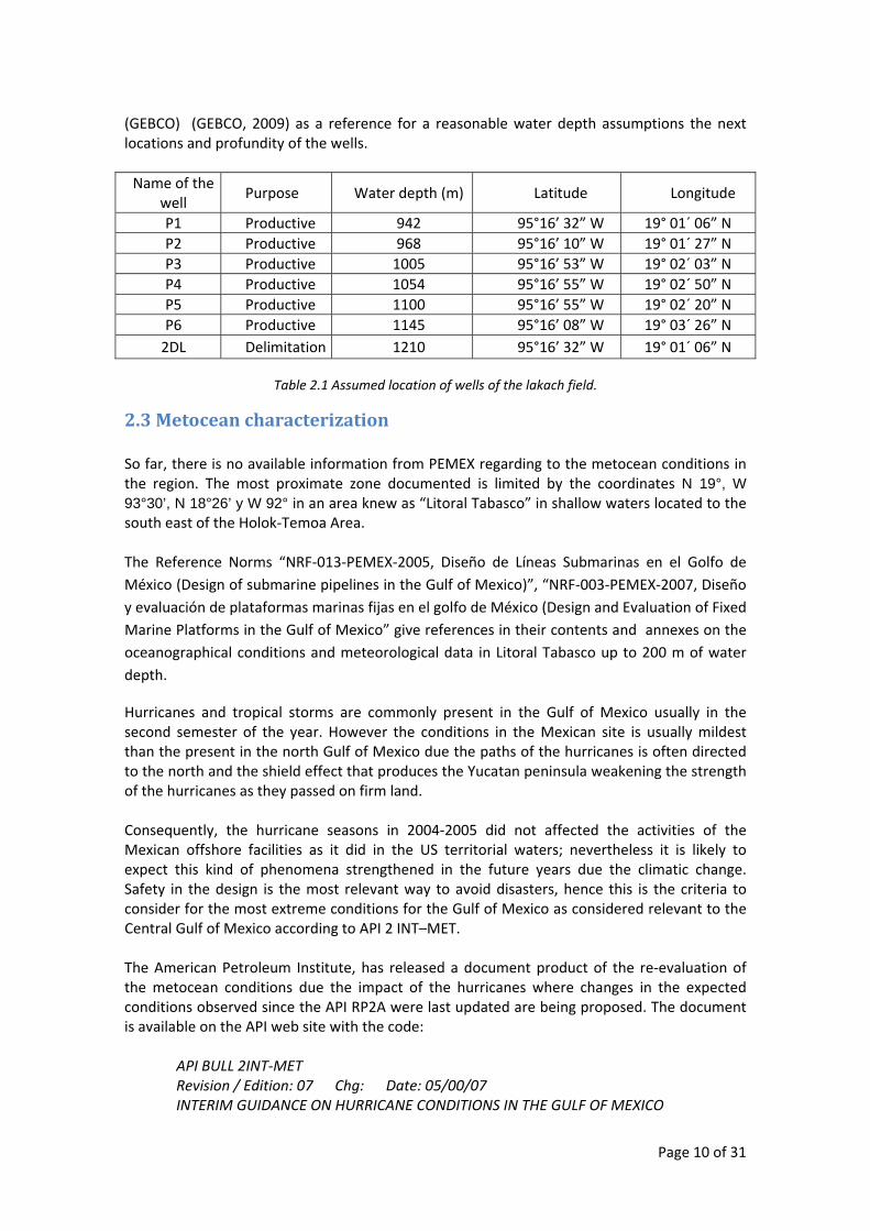
Page 10 of 31
(GEBCO) (GEBCO, 2009) as a reference for a reasonable water depth assumptions the next locations and profundity of the wells. Name of the
well Purpose Water depth (m) Latitude Longitude
P1 Productive 942 95°16’ 32” W 19° 01´ 06” N P2 Productive 968 95°16’ 10” W 19° 01´ 27” N P3 Productive 1005 95°16’ 53” W 19° 02´ 03” N P4 Productive 1054 95°16’ 55” W 19° 02´ 50” N P5 Productive 1100 95°16’ 55” W 19° 02´ 20” N P6 Productive 1145 95°16’ 08” W 19° 03´ 26” N 2DL Delimitation 1210 95°16’ 32” W 19° 01´ 06” N
Table 2.1 Assumed location of wells of the lakach field.
2.3 Metocean characterization So far, there is no available information from PEMEX regarding to the metocean conditions in the region. The most proximate zone documented is limited by the coordinates N 19°, W 93°30’, N 18°26’ y W 92° in an area knew as “Litoral Tabasco” in shallow waters located to the south east of the Holok‐Temoa Area. The Reference Norms “NRF‐013‐PEMEX‐2005, Diseño de Líneas Submarinas en el Golfo de México (Design of submarine pipelines in the Gulf of Mexico)”, “NRF‐003‐PEMEX‐2007, Diseño y evaluación de plataformas marinas fijas en el golfo de México (Design and Evaluation of Fixed Marine Platforms in the Gulf of Mexico” give references in their contents and annexes on the oceanographical conditions and meteorological data in Litoral Tabasco up to 200 m of water depth.
Hurricanes and tropical storms are commonly present in the Gulf of Mexico usually in the second semester of the year. However the conditions in the Mexican site is usually mildest than the present in the north Gulf of Mexico due the paths of the hurricanes is often directed to the north and the shield effect that produces the Yucatan peninsula weakening the strength of the hurricanes as they passed on firm land. Consequently, the hurricane seasons in 2004‐2005 did not affected the activities of the Mexican offshore facilities as it did in the US territorial waters; nevertheless it is likely to expect this kind of phenomena strengthened in the future years due the climatic change. Safety in the design is the most relevant way to avoid disasters, hence this is the criteria to consider for the most extreme conditions for the Gulf of Mexico as considered relevant to the Central Gulf of Mexico according to API 2 INT–MET. The American Petroleum Institute, has released a document product of the re‐evaluation of the metocean conditions due the impact of the hurricanes where changes in the expected conditions observed since the API RP2A were last updated are being proposed. The document is available on the API web site with the code:
API BULL 2INT‐MET Revision / Edition: 07 Chg: Date: 05/00/07
INTERIM GUIDANCE ON HURRICANE CONDITIONS IN THE GULF OF MEXICO
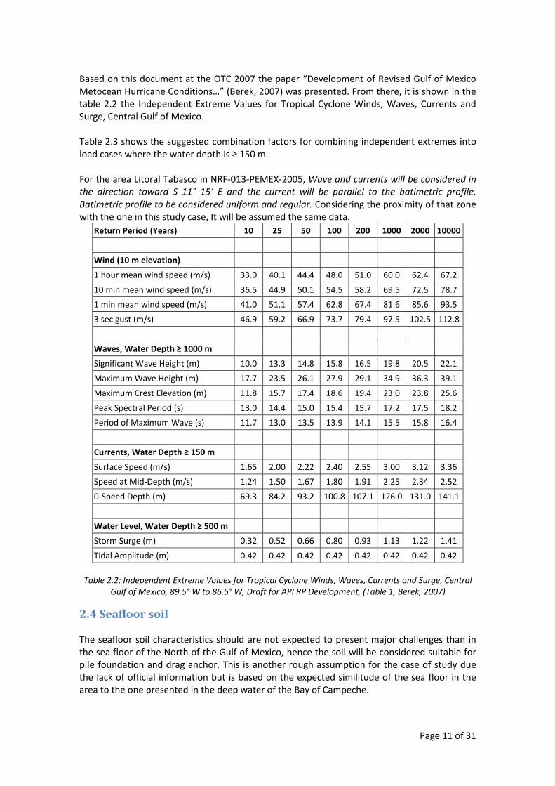
Page 11 of 31
Based on this document at the OTC 2007 the paper “Development of Revised Gulf of Mexico Metocean Hurricane Conditions…” (Berek, 2007) was presented. From there, it is shown in the table 2.2 the Independent Extreme Values for Tropical Cyclone Winds, Waves, Currents and Surge, Central Gulf of Mexico. Table 2.3 shows the suggested combination factors for combining independent extremes into load cases where the water depth is ≥ 150 m. For the area Litoral Tabasco in NRF‐013‐PEMEX‐2005, Wave and currents will be considered in the direction toward S 11° 15’ E and the current will be parallel to the batimetric profile. Batimetric profile to be considered uniform and regular. Considering the proximity of that zone with the one in this study case, It will be assumed the same data.
Return Period (Years) 10 25 50 100 200 1000 2000 10000
Wind (10 m elevation)
1 hour mean wind speed (m/s) 33.0 40.1 44.4 48.0 51.0 60.0 62.4 67.2
10 min mean wind speed (m/s) 36.5 44.9 50.1 54.5 58.2 69.5 72.5 78.7
1 min mean wind speed (m/s) 41.0 51.1 57.4 62.8 67.4 81.6 85.6 93.5
3 sec gust (m/s) 46.9 59.2 66.9 73.7 79.4 97.5 102.5 112.8
Waves, Water Depth ≥ 1000 m
Significant Wave Height (m) 10.0 13.3 14.8 15.8 16.5 19.8 20.5 22.1
Maximum Wave Height (m) 17.7 23.5 26.1 27.9 29.1 34.9 36.3 39.1
Maximum Crest Elevation (m) 11.8 15.7 17.4 18.6 19.4 23.0 23.8 25.6
Peak Spectral Period (s) 13.0 14.4 15.0 15.4 15.7 17.2 17.5 18.2
Period of Maximum Wave (s) 11.7 13.0 13.5 13.9 14.1 15.5 15.8 16.4
Currents, Water Depth ≥ 150 m
Surface Speed (m/s) 1.65 2.00 2.22 2.40 2.55 3.00 3.12 3.36
Speed at Mid‐Depth (m/s) 1.24 1.50 1.67 1.80 1.91 2.25 2.34 2.52
0‐Speed Depth (m) 69.3 84.2 93.2 100.8 107.1 126.0 131.0 141.1
Water Level, Water Depth ≥ 500 m
Storm Surge (m) 0.32 0.52 0.66 0.80 0.93 1.13 1.22 1.41
Tidal Amplitude (m) 0.42 0.42 0.42 0.42 0.42 0.42 0.42 0.42
Table 2.2: Independent Extreme Values for Tropical Cyclone Winds, Waves, Currents and Surge, Central Gulf of Mexico, 89.5° W to 86.5° W, Draft for API RP Development, (Table 1, Berek, 2007)
2.4 Seafloor soil The seafloor soil characteristics should are not expected to present major challenges than in the sea floor of the North of the Gulf of Mexico, hence the soil will be considered suitable for pile foundation and drag anchor. This is another rough assumption for the case of study due the lack of official information but is based on the expected similitude of the sea floor in the area to the one presented in the deep water of the Bay of Campeche.
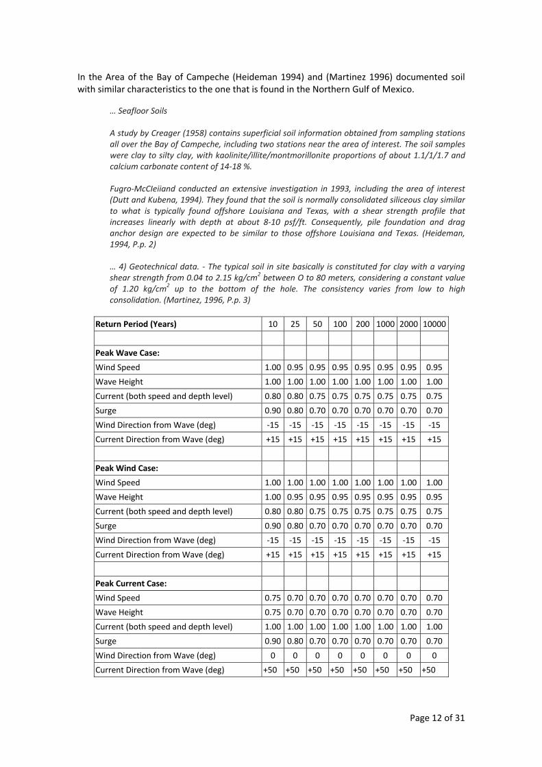
Page 12 of 31
In the Area of the Bay of Campeche (Heideman 1994) and (Martinez 1996) documented soil with similar characteristics to the one that is found in the Northern Gulf of Mexico.
… Seafloor Soils A study by Creager (1958) contains superficial soil information obtained from sampling stations all over the Bay of Campeche, including two stations near the area of interest. The soil samples were clay to silty clay, with kaolinite/illite/montmorillonite proportions of about 1.1/1/1.7 and calcium carbonate content of 14‐18 %. Fugro‐McCIeiiand conducted an extensive investigation in 1993, including the area of interest (Dutt and Kubena, 1994). They found that the soil is normally consolidated siliceous clay similar to what is typically found offshore Louisiana and Texas, with a shear strength profile that increases linearly with depth at about 8‐10 psf/ft. Consequently, pile foundation and drag anchor design are expected to be similar to those offshore Louisiana and Texas. (Heideman, 1994, P.p. 2) … 4) Geotechnical data. ‐ The typical soil in site basically is constituted for clay with a varying shear strength from 0.04 to 2.15 kg/cm2 between O to 80 meters, considering a constant value of 1.20 kg/cm2 up to the bottom of the hole. The consistency varies from low to high consolidation. (Martinez, 1996, P.p. 3)
Return Period (Years) 10 25 50 100 200 1000 2000 10000
Peak Wave Case:
Wind Speed 1.00 0.95 0.95 0.95 0.95 0.95 0.95 0.95
Wave Height 1.00 1.00 1.00 1.00 1.00 1.00 1.00 1.00
Current (both speed and depth level) 0.80 0.80 0.75 0.75 0.75 0.75 0.75 0.75
Surge 0.90 0.80 0.70 0.70 0.70 0.70 0.70 0.70
Wind Direction from Wave (deg) ‐15 ‐15 ‐15 ‐15 ‐15 ‐15 ‐15 ‐15
Current Direction from Wave (deg) +15 +15 +15 +15 +15 +15 +15 +15
Peak Wind Case:
Wind Speed 1.00 1.00 1.00 1.00 1.00 1.00 1.00 1.00
Wave Height 1.00 0.95 0.95 0.95 0.95 0.95 0.95 0.95
Current (both speed and depth level) 0.80 0.80 0.75 0.75 0.75 0.75 0.75 0.75
Surge 0.90 0.80 0.70 0.70 0.70 0.70 0.70 0.70
Wind Direction from Wave (deg) ‐15 ‐15 ‐15 ‐15 ‐15 ‐15 ‐15 ‐15
Current Direction from Wave (deg) +15 +15 +15 +15 +15 +15 +15 +15
Peak Current Case:
Wind Speed 0.75 0.70 0.70 0.70 0.70 0.70 0.70 0.70
Wave Height 0.75 0.70 0.70 0.70 0.70 0.70 0.70 0.70
Current (both speed and depth level) 1.00 1.00 1.00 1.00 1.00 1.00 1.00 1.00
Surge 0.90 0.80 0.70 0.70 0.70 0.70 0.70 0.70
Wind Direction from Wave (deg) 0 0 0 0 0 0 0 0
Current Direction from Wave (deg) +50 +50 +50 +50 +50 +50 +50 +50
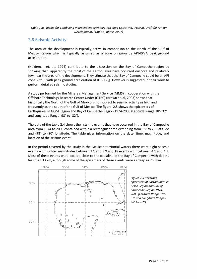
Page 13 of 31
Table 2.3: Factors for Combining Independent Extremes into Load Cases, WD ≥150 m, Draft for API RP Development, (Table 6, Berek, 2007)
2.5 Seismic Activity The area of the development is typically active in comparison to the North of the Gulf of Mexico Region which is typically assumed as a Zone 0 region by API‐RP2A peak ground acceleration. (Heideman et. al., 1994) contribute to the discussion on the Bay of Campeche region by showing that apparently the most of the earthquakes have occurred onshore and relatively few near the area of the development. They stimate that the Bay of Campeche could be an API Zone 2 to 3 with peak ground acceleration of 0.1‐0.2 g. However is suggested in their work to perform detailed seismic studies. A study performed for the Minerals Management Service (MMS) in cooperation with the Offshore Technology Research Center Under (OTRC) (Brown et. al, 2003) shows that historically the North of the Gulf of Mexico is not subject to seismic activity as high and frequently as the south of the Gulf of Mexico. The figure 2.5 shows the epicenters of Earthquakes in GOM Region and Bay of Campeche Region 1974‐2003 (Latitude Range 18°‐ 32° and Longitude Range ‐98° to ‐82°). The data of the table 2.4 shows the lists the events that have occurred in the Bay of Campeche area from 1974 to 2003 contained within a rectangular area extending from 18° to 20° latitude and ‐98° to ‐90° longitude. The table gives information on the date, time, magnitude, and location of the seismic event. In the period covered by the study in the Mexican territorial waters there were eight seismic events with Richter magnitudes between 3.1 and 3.9 and 18 events with between 4.1 and 4.7. Most of these events were located close to the coastline in the Bay of Campeche with depths less than 33 km, although some of the epicenters of these events were as deep as 250 km.
Figure 2.5 Recorded epicenters of Earthquakes in GOM Region and Bay of Campeche Region 1974‐2003 (Latitude Range 18°‐ 32° and Longitude Range ‐98° to ‐82°)
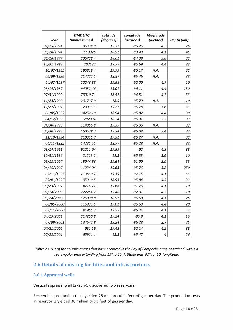
Page 14 of 31
Year TIME UTC
(hhmmss.mm) Latitude (degrees)
Longitude (degrees)
Magnitude (Richter) Depth (km)
07/25/1974 95338.9 19.37 ‐96.25 4.5 76
09/20/1974 113326 18.91 ‐93.49 4.1 45
08/28/1977 235738.4 18.61 ‐94.39 3.8 33
12/31/1983 202132 18.77 ‐95.69 4.4 33
10/07/1985 195819.4 19.75 ‐96.17 N.A. 33
06/09/1986 214222.1 18.57 ‐95.46 N.A. 33
04/07/1987 20246.58 19.58 ‐92.09 4.7 10
08/14/1987 94032.46 19.01 ‐96.11 4.4 130
07/31/1990 73010.71 18.52 ‐94.51 4.7 33
11/23/1990 201737.9 18.5 ‐95.79 N.A. 10
11/27/1991 120033.3 19.22 ‐95.78 3.6 33
06/05/1992 34252.19 18.94 ‐95.82 4.4 39
04/12/1993 202034 18.74 ‐95.31 3.7 33
04/30/1993 114856.8 19.39 ‐96.06 N.A. 33
04/30/1993 150538.7 19.34 ‐96.08 3.4 33
11/10/1994 210315.7 19.31 ‐95.27 N.A. 33
04/11/1995 14231.51 18.77 ‐95.28 N.A. 33
03/14/1996 91211.94 19.53 ‐92 4.3 33
10/31/1996 21223.2 19.3 ‐95.33 3.6 10
03/18/1997 15944.66 19.64 ‐91.99 3.9 33
04/15/1997 11234.04 19.63 ‐95.76 3.8 250
07/11/1997 210830.7 19.39 ‐92.15 4.1 33
09/01/1997 105019.5 18.94 ‐95.84 4.3 33
09/23/1997 4716.77 19.66 ‐91.76 4.1 10
01/14/2000 222254.2 19.46 ‐92.01 4.3 10
03/24/2000 175830.8 18.91 ‐95.58 4.1 26
06/05/2000 115931.5 19.01 ‐95.68 4.4 20
08/11/2000 81955.3 19.55 ‐96.41 4.1 4
04/19/2001 214250.8 19.24 ‐95.9 4.1 16
07/09/2001 134642.8 19.24 ‐96.28 3.7 25
07/21/2001 951.19 19.42 ‐92.14 4.2 33
07/23/2001 65921.1 18.5 ‐95.47 4 26
Table 2.4 List of the seismic events that have occurred in the Bay of Campeche area, contained within a rectangular area extending from 18° to 20° latitude and ‐98° to ‐90° longitude.
2.6 Details of existing facilities and infrastructure.
2.6.1 Appraisal wells Vertical appraisal well Lakach‐1 discovered two reservoirs. Reservoir 1 production tests yielded 25 million cubic feet of gas per day. The production tests in reservoir 2 yielded 30 million cubic feet of gas per day.
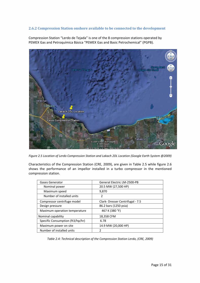
Page 15 of 31
2.6.2 Compression Station onshore available to be connected to the development Compression Station “Lerdo de Tejada” is one of the 8 compression stations operated by PEMEX Gas and Petroquímica Básica “PEMEX Gas and Basic Petrochemical” (PGPB).
Figure 2.5 Location of Lerdo Compression Station and Lakach 2DL Location (Google Earth System @2009) Characteristics of the Compression Station (CRE, 2009), are given in Table 2.5 while figure 2.6 shows the performance of an impellor installed in a turbo compressor in the mentioned compression station.
Gases Generator General Electric LM‐2500‐PB Nominal power 20.5 MW (27,500 HP) Maximum speed 9,870 Number of installed units 2
Compressor centrifuge model Clark‐ Dresser Centrifugal ‐ 7.5Design pressure 86.2 bars (1250 psia)
Maximum operation temperature 467 K (380 °F)
Nominal capability 18,358 CFMSpecific Consumption (ft3/hp/hr) 6.78
Maximum power on site 14.9 MW (20,000 HP)Number of installed units 2
Table 2.4: Technical description of the Compression Station Lerdo, (CRE, 2009)
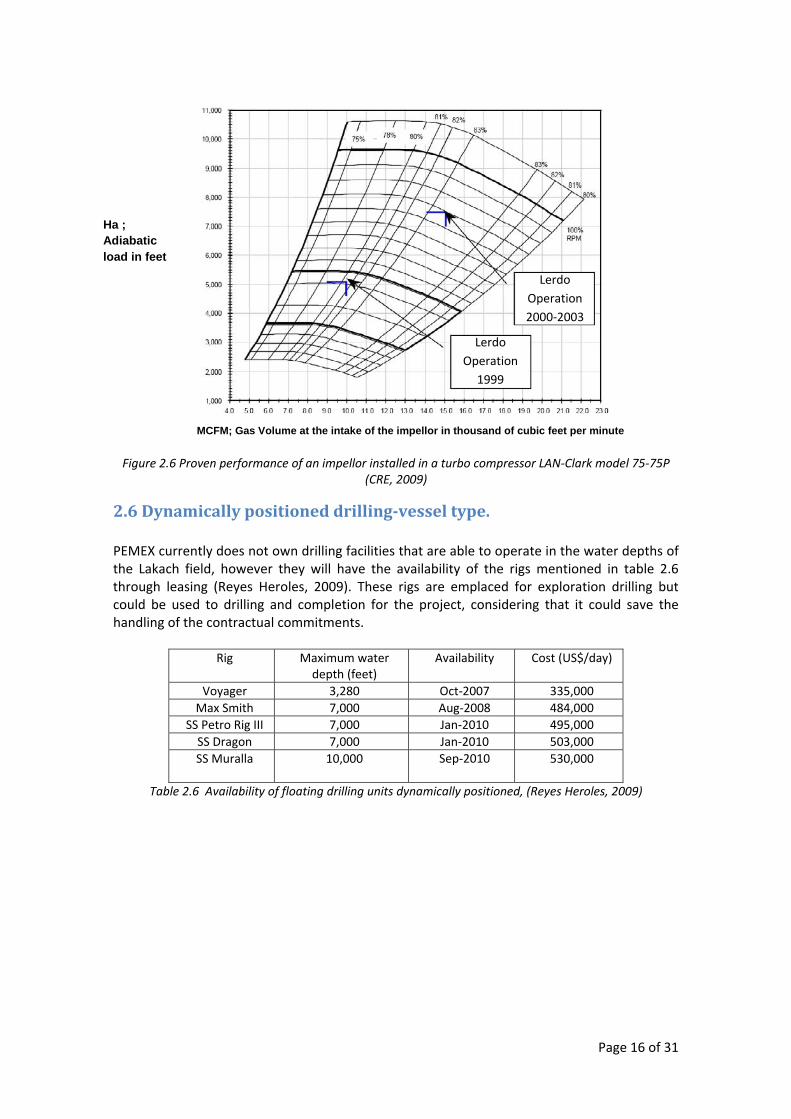
Page 16 of 31
Figure 2.6 Proven performance of an impellor installed in a turbo compressor LAN‐Clark model 75‐75P (CRE, 2009)
2.6 Dynamically positioned drillingvessel type. PEMEX currently does not own drilling facilities that are able to operate in the water depths of the Lakach field, however they will have the availability of the rigs mentioned in table 2.6 through leasing (Reyes Heroles, 2009). These rigs are emplaced for exploration drilling but could be used to drilling and completion for the project, considering that it could save the handling of the contractual commitments.
Rig Maximum water depth (feet)
Availability Cost (US$/day)
Voyager 3,280 Oct‐2007 335,000 Max Smith 7,000 Aug‐2008 484,000
SS Petro Rig III 7,000 Jan‐2010 495,000 SS Dragon 7,000 Jan‐2010 503,000 SS Muralla 10,000 Sep‐2010 530,000
Table 2.6 Availability of floating drilling units dynamically positioned, (Reyes Heroles, 2009)
Lerdo Operation 2000‐2003
Lerdo Operation
1999
MCFM; Gas Volume at the intake of the impellor in thousand of cubic feet per minute
Ha ; Adiabatic load in feet
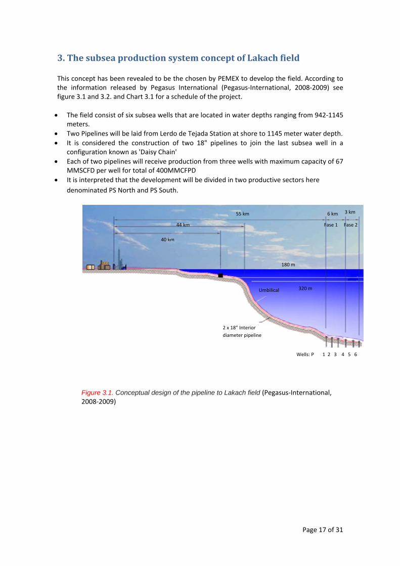
Page 17 of 31
3. The subsea production system concept of Lakach field This concept has been revealed to be the chosen by PEMEX to develop the field. According to the information released by Pegasus International (Pegasus‐International, 2008‐2009) see figure 3.1 and 3.2. and Chart 3.1 for a schedule of the project. • The field consist of six subsea wells that are located in water depths ranging from 942‐1145
meters. • Two Pipelines will be laid from Lerdo de Tejada Station at shore to 1145 meter water depth. • It is considered the construction of two 18" pipelines to join the last subsea well in a
configuration known as 'Daisy Chain' • Each of two pipelines will receive production from three wells with maximum capacity of 67
MMSCFD per well for total of 400MMCFPD • It is interpreted that the development will be divided in two productive sectors here
denominated PS North and PS South.
Figure 3.1. Conceptual design of the pipeline to Lakach field (Pegasus‐International, 2008‐2009)
Umbilical 320 m
180 m
Fase 1 Fase 2
6 km 3 km
44 km
40 km
2 x 18” Interior diameter pipeline
55 km
Wells: P 1 2 3 4 5 6
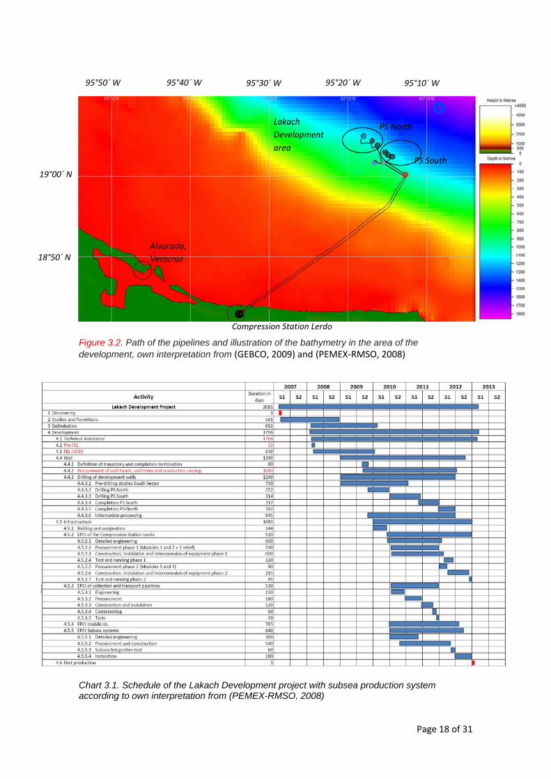
Page 18 of 31
Figure 3.2. Path of the pipelines and illustration of the bathymetry in the area of the development, own interpretation from (GEBCO, 2009) and (PEMEX‐RMSO, 2008)
Chart 3.1. Schedule of the Lakach Development project with subsea production system according to own interpretation from (PEMEX-RMSO, 2008)
Compression Station Lerdo
Lakach Development area
PS South
PS North
95°10´ W 95°20´ W95°30´ W95°40´ W 95°50´ W
19°00´ N
18°50´ N Alvarado, Veracruz
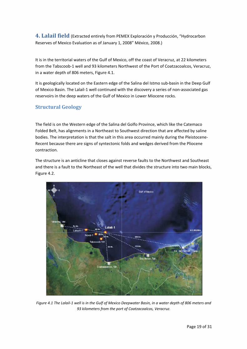
Page 19 of 31
4. Lalail field (Extracted entirely from PEMEX Exploración y Producción, “Hydrocarbon
Reserves of Mexico Evaluation as of January 1, 2008” México, 2008.)
It is in the territorial waters of the Gulf of Mexico, off the coast of Veracruz, at 22 kilometers from the Tabscoob‐1 well and 93 kilometers Northwest of the Port of Coatzacoalcos, Veracruz, in a water depth of 806 meters, Figure 4.1.
It is geologically located on the Eastern edge of the Salina del Istmo sub‐basin in the Deep Gulf of Mexico Basin. The Lalail‐1 well continued with the discovery a series of non‐associated gas reservoirs in the deep waters of the Gulf of Mexico in Lower Miocene rocks.
Structural Geology
The field is on the Western edge of the Salina del Golfo Province, which like the Catemaco Folded Belt, has alignments in a Northeast to Southwest direction that are affected by saline bodies. The interpretation is that the salt in this area occurred mainly during the Pleistocene‐ Recent because there are signs of syntectonic folds and wedges derived from the Pliocene contraction.
The structure is an anticline that closes against reverse faults to the Northwest and Southeast and there is a fault to the Northeast of the well that divides the structure into two main blocks, Figure 4.2.
Figure 4.1 The Lalail‐1 well is in the Gulf of Mexico Deepwater Basin, in a water depth of 806 meters and 93 kilometers from the port of Coatzacoalcos, Veracruz.
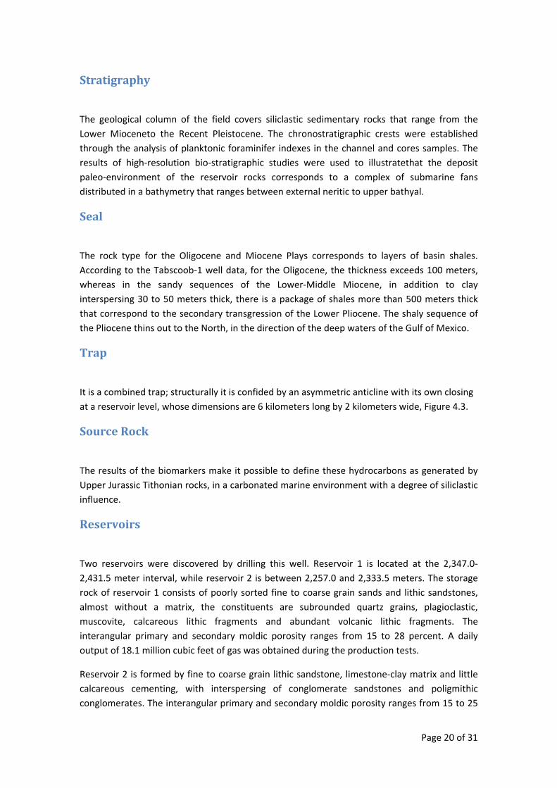
Page 20 of 31
Stratigraphy
The geological column of the field covers siliclastic sedimentary rocks that range from the Lower Mioceneto the Recent Pleistocene. The chronostratigraphic crests were established through the analysis of planktonic foraminifer indexes in the channel and cores samples. The results of high‐resolution bio‐stratigraphic studies were used to illustratethat the deposit paleo‐environment of the reservoir rocks corresponds to a complex of submarine fans distributed in a bathymetry that ranges between external neritic to upper bathyal.
Seal
The rock type for the Oligocene and Miocene Plays corresponds to layers of basin shales. According to the Tabscoob‐1 well data, for the Oligocene, the thickness exceeds 100 meters, whereas in the sandy sequences of the Lower‐Middle Miocene, in addition to clay interspersing 30 to 50 meters thick, there is a package of shales more than 500 meters thick that correspond to the secondary transgression of the Lower Pliocene. The shaly sequence of the Pliocene thins out to the North, in the direction of the deep waters of the Gulf of Mexico.
Trap
It is a combined trap; structurally it is confided by an asymmetric anticline with its own closing at a reservoir level, whose dimensions are 6 kilometers long by 2 kilometers wide, Figure 4.3.
Source Rock
The results of the biomarkers make it possible to define these hydrocarbons as generated by Upper Jurassic Tithonian rocks, in a carbonated marine environment with a degree of siliclastic influence.
Reservoirs
Two reservoirs were discovered by drilling this well. Reservoir 1 is located at the 2,347.0‐2,431.5 meter interval, while reservoir 2 is between 2,257.0 and 2,333.5 meters. The storage rock of reservoir 1 consists of poorly sorted fine to coarse grain sands and lithic sandstones, almost without a matrix, the constituents are subrounded quartz grains, plagioclastic, muscovite, calcareous lithic fragments and abundant volcanic lithic fragments. The interangular primary and secondary moldic porosity ranges from 15 to 28 percent. A daily output of 18.1 million cubic feet of gas was obtained during the production tests.
Reservoir 2 is formed by fine to coarse grain lithic sandstone, limestone‐clay matrix and little calcareous cementing, with interspersing of conglomerate sandstones and poligmithic conglomerates. The interangular primary and secondary moldic porosity ranges from 15 to 25
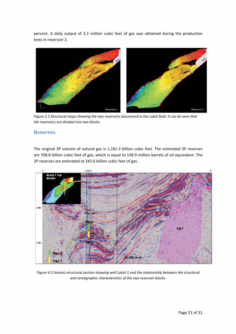
Page 21 of 31
percent. A daily output of 3.2 million cubic feet of gas was obtained during the production tests in reservoir 2.
Figure 5.2 Structural maps showing the two reservoirs discovered in the Lalail field. It can be seen that the reservoirs are divided into two blocks.
Reserves
The original 3P volume of natural gas is 1,181.3 billion cubic feet. The estimated 3P reserves are 708.8 billion cubic feet of gas, which is equal to 138.9 million barrels of oil equivalent. The 2P reserves are estimated at 242.6 billion cubic feet of gas.
Figure 4.3 Seismic‐structural section showing well Lalail‐1 and the relationship between the structural and stratigraphic characteristics of the two reservoir blocks.
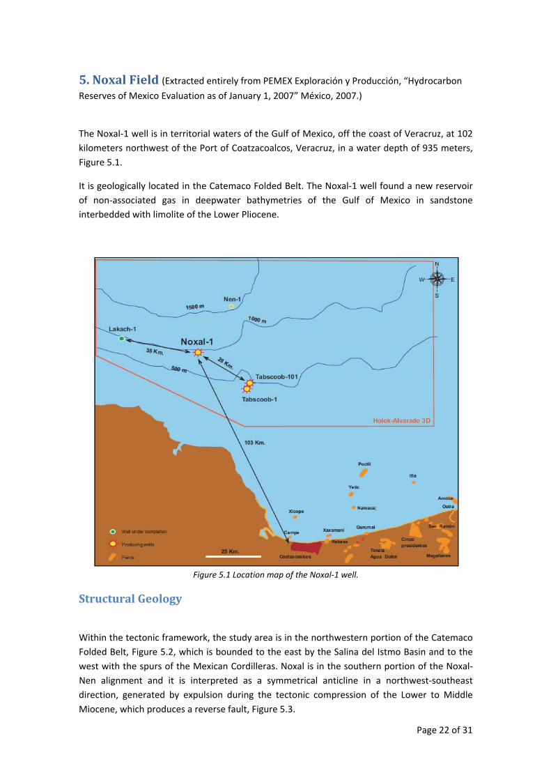
Page 22 of 31
5. Noxal Field (Extracted entirely from PEMEX Exploración y Producción, “Hydrocarbon
Reserves of Mexico Evaluation as of January 1, 2007” México, 2007.)
The Noxal‐1 well is in territorial waters of the Gulf of Mexico, off the coast of Veracruz, at 102 kilometers northwest of the Port of Coatzacoalcos, Veracruz, in a water depth of 935 meters, Figure 5.1.
It is geologically located in the Catemaco Folded Belt. The Noxal‐1 well found a new reservoir of non‐associated gas in deepwater bathymetries of the Gulf of Mexico in sandstone interbedded with limolite of the Lower Pliocene.
Figure 5.1 Location map of the Noxal‐1 well.
Structural Geology
Within the tectonic framework, the study area is in the northwestern portion of the Catemaco Folded Belt, Figure 5.2, which is bounded to the east by the Salina del Istmo Basin and to the west with the spurs of the Mexican Cordilleras. Noxal is in the southern portion of the Noxal‐Nen alignment and it is interpreted as a symmetrical anticline in a northwest‐southeast direction, generated by expulsion during the tectonic compression of the Lower to Middle Miocene, which produces a reverse fault, Figure 5.3.
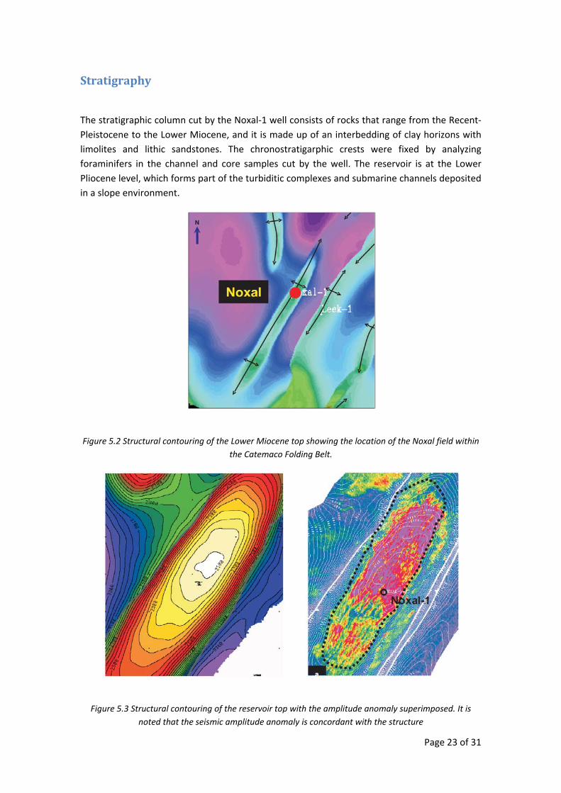
Page 23 of 31
Stratigraphy
The stratigraphic column cut by the Noxal‐1 well consists of rocks that range from the Recent‐Pleistocene to the Lower Miocene, and it is made up of an interbedding of clay horizons with limolites and lithic sandstones. The chronostratigarphic crests were fixed by analyzing foraminifers in the channel and core samples cut by the well. The reservoir is at the Lower Pliocene level, which forms part of the turbiditic complexes and submarine channels deposited in a slope environment.
Figure 5.2 Structural contouring of the Lower Miocene top showing the location of the Noxal field within the Catemaco Folding Belt.
Figure 5.3 Structural contouring of the reservoir top with the amplitude anomaly superimposed. It is noted that the seismic amplitude anomaly is concordant with the structure
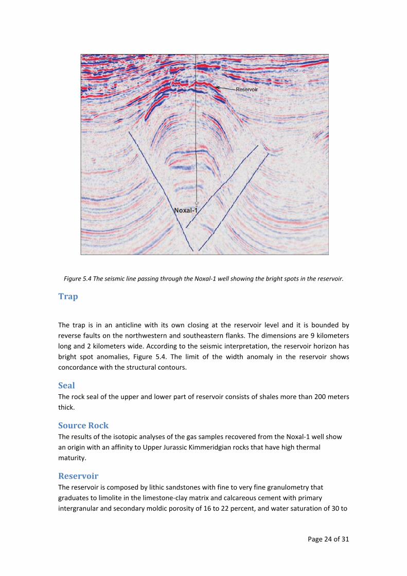
Page 24 of 31
Figure 5.4 The seismic line passing through the Noxal‐1 well showing the bright spots in the reservoir.
Trap
The trap is in an anticline with its own closing at the reservoir level and it is bounded by reverse faults on the northwestern and southeastern flanks. The dimensions are 9 kilometers long and 2 kilometers wide. According to the seismic interpretation, the reservoir horizon has bright spot anomalies, Figure 5.4. The limit of the width anomaly in the reservoir shows concordance with the structural contours.
Seal The rock seal of the upper and lower part of reservoir consists of shales more than 200 meters thick.
Source Rock The results of the isotopic analyses of the gas samples recovered from the Noxal‐1 well show an origin with an affinity to Upper Jurassic Kimmeridgian rocks that have high thermal maturity.
Reservoir The reservoir is composed by lithic sandstones with fine to very fine granulometry that graduates to limolite in the limestone‐clay matrix and calcareous cement with primary intergranular and secondary moldic porosity of 16 to 22 percent, and water saturation of 30 to
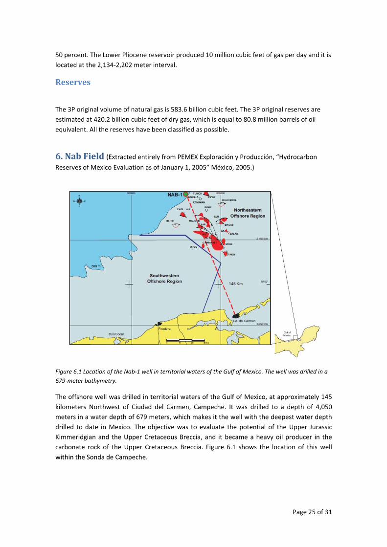
Page 25 of 31
50 percent. The Lower Pliocene reservoir produced 10 million cubic feet of gas per day and it is located at the 2,134‐2,202 meter interval.
Reserves
The 3P original volume of natural gas is 583.6 billion cubic feet. The 3P original reserves are estimated at 420.2 billion cubic feet of dry gas, which is equal to 80.8 million barrels of oil equivalent. All the reserves have been classified as possible.
6. Nab Field (Extracted entirely from PEMEX Exploración y Producción, “Hydrocarbon
Reserves of Mexico Evaluation as of January 1, 2005” México, 2005.)
Figure 6.1 Location of the Nab‐1 well in territorial waters of the Gulf of Mexico. The well was drilled in a 679‐meter bathymetry.
The offshore well was drilled in territorial waters of the Gulf of Mexico, at approximately 145 kilometers Northwest of Ciudad del Carmen, Campeche. It was drilled to a depth of 4,050 meters in a water depth of 679 meters, which makes it the well with the deepest water depth drilled to date in Mexico. The objective was to evaluate the potential of the Upper Jurassic Kimmeridgian and the Upper Cretaceous Breccia, and it became a heavy oil producer in the carbonate rock of the Upper Cretaceous Breccia. Figure 6.1 shows the location of this well within the Sonda de Campeche.
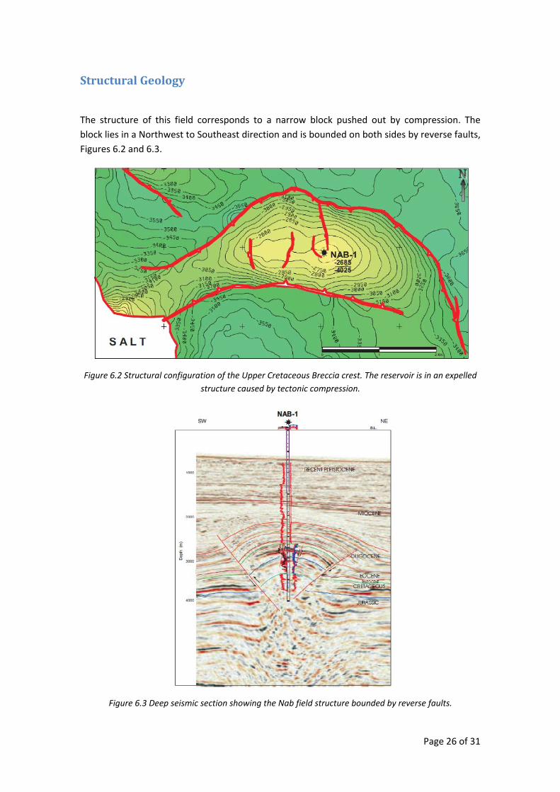
Page 26 of 31
Structural Geology
The structure of this field corresponds to a narrow block pushed out by compression. The block lies in a Northwest to Southeast direction and is bounded on both sides by reverse faults, Figures 6.2 and 6.3.
Figure 6.2 Structural configuration of the Upper Cretaceous Breccia crest. The reservoir is in an expelled structure caused by tectonic compression.
Figure 6.3 Deep seismic section showing the Nab field structure bounded by reverse faults.
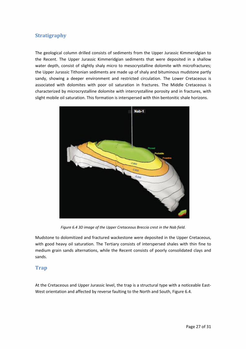
Page 27 of 31
Stratigraphy
The geological column drilled consists of sediments from the Upper Jurassic Kimmeridgian to the Recent. The Upper Jurassic Kimmeridgian sediments that were deposited in a shallow water depth, consist of slightly shaly micro to mesocrystalline dolomite with microfractures; the Upper Jurassic Tithonian sediments are made up of shaly and bituminous mudstone partly sandy, showing a deeper environment and restricted circulation. The Lower Cretaceous is associated with dolomites with poor oil saturation in fractures. The Middle Cretaceous is characterized by microcrystalline dolomite with intercrystalline porosity and in fractures, with slight mobile oil saturation. This formation is interspersed with thin bentonitic shale horizons.
Figure 6.4 3D image of the Upper Cretaceous Breccia crest in the Nab field.
Mudstone to dolomitized and fractured wackestone were deposited in the Upper Cretaceous, with good heavy oil saturation. The Tertiary consists of interspersed shales with thin fine to medium grain sands alternations, while the Recent consists of poorly consolidated clays and sands.
Trap
At the Cretaceous and Upper Jurassic level, the trap is a structural type with a noticeable East‐West orientation and affected by reverse faulting to the North and South, Figure 6.4.
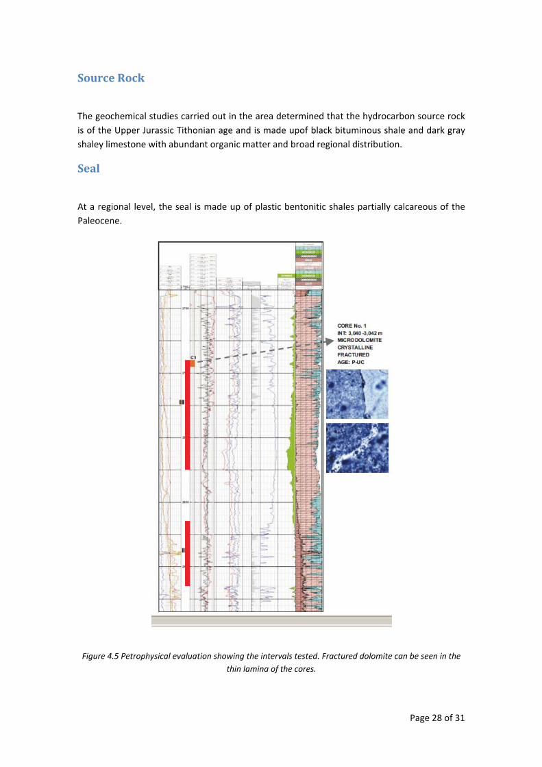
Page 28 of 31
Source Rock
The geochemical studies carried out in the area determined that the hydrocarbon source rock is of the Upper Jurassic Tithonian age and is made upof black bituminous shale and dark gray shaley limestone with abundant organic matter and broad regional distribution.
Seal
At a regional level, the seal is made up of plastic bentonitic shales partially calcareous of the Paleocene.
Figure 4.5 Petrophysical evaluation showing the intervals tested. Fractured dolomite can be seen in the thin lamina of the cores.
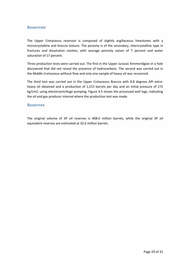
Page 29 of 31
Reservoir
The Upper Cretaceous reservoir is composed of slightly argillaceous limestones with a microcrystalline and breccia texture. The porosity is of the secondary, intercrystalline type in fractures and dissolution cavities, with average porosity values of 7 percent and water saturation of 17 percent.
Three production tests were carried out. The first in the Upper Jurassic Kimmeridgian in a hole discovered that did not reveal the presence of hydrocarbons. The second was carried out in the Middle Cretaceous without flow and only one sample of heavy oil was recovered.
The third test was carried out in the Upper Cretaceous Breccia with 8.8 degrees API extra‐heavy oil obtained and a production of 1,215 barrels per day and an initial pressure of 272 kg/cm2, using electorcentrifuge pumping. Figure 4.5 shows the processed well logs, indicating the oil and gas producer interval where the production test was made.
Reserves
The original volume of 3P oil reserves is 408.0 million barrels, while the original 3P oil equivalent reserves are estimated at 32.6 million barrels.
Page 30 of 31
REFERENCES:
• American Petroleum Institute (API), “Interim Guidance on Hurricane Conditions in the Gulf of Mexico”, Bulletin 2INT‐MET, USA, 2007.
• Brown L.A., M.S., Bracci J.M., Hueste M.B., Murff J.D. Texas A&M University, “Assessment of Seismic Risk for Subsea Production Systems in the Gulf of Mexico”, Final Project Report Prepared for the Minerals Management Service, Under the MMS/OTRC Cooperative Research Agreement 1435‐01‐99‐CA‐31003, Task Order 18204, Project Number 422, USA, December2003.
• Berek, E.P., ExxonMobil; Cooper, C.K. Chevron; Driver, D.B., BP; Heideman J. C. and Mitchell, D.A ExxonMobil, Stear, J.D., Chevron; and Vogel, M.J., Shell International EP “Development of Revised Gulf of Mexico Metocean Hurricane Conditions for Reference by API Recommended Practices”; Paper OTC 18903, Offshore Technology Conference, 2007.
• CRE (Comisión Reguladora de Energía), “Permiso de transporte de gas natural numero: G/061/TRA/99 Anexo 3 Características de tecnología, diseño, ingeniería y construcción Apéndice 3.1, Memoria técnico‐descriptiva del sistema de transporte. Consulted on internet at http://www.cre.gob.mx/registro/permisos/gas/Anexos/061tra99x/apn31.pdf, last visited August 28th 2009.
• GEBCO, “General Bathymetric Chart of the Oceans, The GEBCO_08 Grid, version 20090212,” http://www.gebco.net, 2009.
• Morales C. “Deep Water Exploration Strategy” Presentation of the Pemex Exploración y Producción General Director, Carlos A. Morales Gil in the Offshore Technology Conference, May 7th, 2009. Consulted in the web page
• Pegasus‐International, “Project description Lakach” consulted in the web page http://www.pegasus‐international.com/uploads/portfolio_letter_pdf_223.pdf, Pegasus International web site, August 13th, 2009.
• PEMEX Exploración y Producción, “Hydrocarbon Reserves of Mexico Evaluation as of January 1, 2005” México, 2005.
• PEMEX Exploración y Producción, “Hydrocarbon Reserves of Mexico Evaluation as of January 1, 2007” México, 2007.
• PEMEX Exploración y Producción, “Hydrocarbon Reserves of Mexico Evaluation as of January 1, 2008” México, 2008.
• PEMEX‐RMSO Exploración y Producción Región Marina Suroeste, “Resumen ejecutivo, Manifestación de impacto ambiental modalidad regional proyecto Lakach” México, 2008.
• PEMEX Exploración y Producción, “Licitación pública internacional TLC No. 18575088‐018‐08 anexo B‐1", México, 2008.
• PEMEX Exploración y Producción, “NRF‐013‐PEMEX‐2005, Diseño de Líneas Submarinas en el Golfo de México.” Comité de Normalización de Petróleos Mexicanos y Organismos Subsidiarios, México, 2005.
• PEMEX Exploración y Producción, “NRF‐003‐PEMEX‐2007 Diseño y evaluación de plataformas marinas fijas en el golfo de México.” Comité de Normalización de Petróleos Mexicanos y Organismos Subsidiarios, México, 2007.
• Reyes Heroles J.G.G., “Aspectos relevantes en materia de exploración y producción de hidrocarburos” Comparecencia del Director General de Petróleos Mexicanos, en la Comisión de Energía del Senado de la República, January 14th, 2009.
• SENER, Secretaría de Energía, “Prospectiva del mercado de gas natural 2008‐2017”, México, 2008.

Page 31 of 31
• SENER, Secretaría de Energía, “Segundo informe de labores”, México, 2008. • SEMARNAT, Secretaría de Medio Ambiente y Recursos Naturales, “Listado del ingreso
de proyectos y emisión de resolutivos derivados del procedimiento de evaluación de impacto y riesgo ambiental”, Gaceta Ecológica Año VII Separata N° DGIRA/001/09 SEMARNAT/DGIRA México, D. F. January 8th, 2009.
• SPE (Society of Petroleum Engineers), “Guidelines for the Evaluation of Petroleum Reserves and Resources”, USA, 2001.