Rohit Rahi and Jean-Pierre ZigrandArbitrage networks Working paper Original citation: Rahi, Rohit and Zigrand, Jean-Pierre (2008) Arbitrage networks. Rohit Rahi and Jean-Pierre Zigrand, London, UK. (Unpublished) This version available at: http://eprints.lse.ac.uk/4787/ Originally available from http://vishnu.lse.ac.uk/Rohit_Rahi/Homepage.html Available in LSE Research Online: March 2009 © 2007 The Authors LSE has developed LSE Research Online so that users may access research output of the School. Copyright © and Moral Rights for the papers on this site are retained by the individual authors and/or other copyright owners. Users may download and/or print one copy of any article(s) in LSE Research Online to facilitate their private study or for non-commercial research. You may not engage in further distribution of the material or use it for any profit-making activities or any commercial gain. You may freely distribute the URL (http://eprints.lse.ac.uk) of the LSE Research Online website.

Arbitrage Networks∗

by

Rohit Rahi

Department of Finance,

Department of Economics,

and Financial Markets Group,

London School of Economics,

Houghton Street, London WC2A 2AE

and

Jean-Pierre Zigrand

Department of Finance

and Financial Markets Group,

London School of Economics,

Houghton Street, London WC2A 2AE

January 24, 2008.

∗This paper has benefited from comments by Piero Gottardi, Tarun Ramadorai, and Giulia Iori.We also thank seminar participants at the HEC Economics Workshop 2005 in honor of AndreuMas-Colell, the NBER/NSF Decentralization Conference 2006 in Paris and seminar participants atLSE, Bank of England, Venice, Zurich and New Economic School in Moscow.

Abstract

This paper is studies the general equilibrium implications of arbitrage trades bystrategic players in segmented financial markets. Arbitrageurs exploit clienteleeffects and choose to specialize in one category of trades, taking into considera-tion all other arbitrage strategies. This results in an equilibrium network of ar-bitrageurs. The optimal network for arbitrageurs is of the hub-spoke kind. Theequilibrium network, in contrast, is never optimal for arbitrageurs and is neverhub-spoke. The reason is that equilibrium networks suffer from a Prisoner’sDilemma problem that prevents network externalities from being internalized.We show that, as the number of intermediaries grows, equilibrium allocationsconverge to those of the frictionless complete-markets Arrow-Debreu economy.

Journal of Economic Literature classification numbers: G12, D52.

Keywords: Networks, arbitrage, restricted participation.

2

1 Introduction

The Arrow-Debreu-Radner (ADR) model describes a world in which all economicactors are price-takers and in which all claims and commodities are traded on acentralized exchange, with a Walrasian auctioneer determining one market pricevector clearing all markets simultaneously. The simplifications involved in this setuphave allowed the model to become a useful benchmark in economic theory.

Clearly not all actual markets correspond exactly or even approximately to suchan idealization, and we would like to argue in this paper that global financial marketsshould be modeled based upon an extension of the ADR model in at least twodirections.

First, while most retail investors in financial markets can be safely considered tobe price-takers, agents such as universal banks, investment banks, market makers,mutual and hedge fund managers, insurance companies and the like do exert con-siderable influence on markets and must be presumed to be strategic rather thanprice-taking.

Second, not all assets and commodities in the entire world are traded simulta-neously on one single giant exchange. Assets are traded on a variety of tradingposts, such as stock exchanges, options and futures exchanges, as well as over-the-counter (OTC), i.e. in direct and private arms-length transactions bypassing formalexchanges. A large fraction of trades are OTC, and in this category one can includemany derivatives deals, foreign exchange dealings, upstairs trading, block trading,bank loans and deposits, private placements of securities, book building such as inprimary and secondary stock issues, and so forth. We refer to such trading posts asexchanges. As a result, various clienteles trade on different exchanges, and very fewretail clients trade on more than one exchange, let alone on all of them simultane-ously. This invalidates the posit of traditional pricing theory whereby the marginalinvestor in every asset market is the same broadly diversified representative investor.

This market segmentation leads to asset price characteristics distinct from thosethat the ADR model can generate. The obvious example that comes to mind isthe importance of geographic factors. Traders need to be embedded locally in orderto appreciate local market conventions, local demand by clients and to gather localinformation in order to successfully develop a “market feel” and to respond by formu-lating a “market view” (see for instance the survey-based paper by Agnes (2000)).Segmentations do not exclusively arise due to geographic factors. The usefulnessof a general segmentation setup has been recognized long ago, as documented forinstance in the success of the market segmentation hypothesis (Culbertson (1957))and the preferred habitat hypothesis (Modigliani and Sutch (1966)) in fixed incomeanalytics. For example, banks and building societies concentrate a large part of theiractivity at the short end of the interest rate term structure, both for asset-liabilityand for regulatory reasons, while pension funds and insurance companies operateat the long end. More generally, the assumption of market segmentation impliesthat asset prices are determined locally and that as a result overall asset prices need

3

not be contained in the set of no-arbitrage prices. This opens up the possibilityfor some sophisticated players to profit from said opportunities by intermediatingand facilitating trade. These large players, which we shall simply refer to as arbi-trageurs in this paper, have a well-defined objective function even in the presence ofexploitable arbitrage opportunities, since the awareness of a market impact naturallybounds their trades, for else arbitrage opportunities vanish and no profit at all canbe reaped.

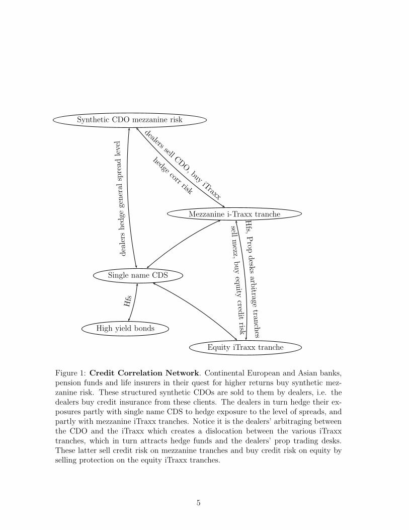
A series of recent papers have tried to empirically quantify the extent to whichstate prices differ across markets. One of the first systematic studies is the paperby Chen and Knez (1995) who consider the mean-square distance between sets ofstate prices on different exchanges. They find that the NYSE and NASDAQ arepriced by sets of state prices which are close in that norm but do not intersect, show-ing that the marginal investors on the two markets are close but distinct. Thereis also a prolific literature on home bias, wherein a national stock market is heldand priced predominantly by national investors (see for instance Lewis (1999) for asurvey). More recently, there have been a number of event studies of changes in thecomposition of the S&P 500 index (see for instance Massa et al. (2005)). Around thetime of the addition a stock to the index, mutual funds benchmarked to the indexhave an incentive to purchase the stock, and their marginal valuations are shown todiffer from those of the market at large. Part of the resulting arbitrage is in factperformed by the managers of the company admitted to the index. Similarly, Daand Gao (2006) provide empirical evidence supporting the view that a sharp rise in afirm’s default likelihood causes a change in its shareholder clientele as mutual fundsdecrease their holdings of the firm’s shares. This liquidity shock is initially absorbedby market-makers before large traders move in to provide the liquidity. The paperby Blackburn et al. (2006) attempts to show that the marginal growth investor isdistinct from the marginal value investor by measuring the different risk aversionparameters priced into the two markets. They find preliminary evidence that themarginal growth investor is indeed less risk averse than the marginal value investor.Gabaix et al. (2007), in a study of the mortgage-backed securities (MBS) market,show that collateralized mortgage obligations (CMOs) are priced not by the marginalinvestor of the broader market whose state prices depend on the aggregate wealth orconsumption of the economy, but by investors wholly specialized in the MBS market.In particular, they find that prepayment risk is priced even though it washes out inthe aggregate. The market price of prepayment risk has a systematic relation withthe marginal utility proxy of the MBS specialist investor. The intermediaries whopurchase the mortgages and transform them into CMOs play the role of our arbi-trageurs. A further illustration of the way the stresses in the credit markets startingin May 2005, initially triggered by concerns about GM and Ford, were transmittedthrough the system show the complex arbitrage web in contemporary credit corre-lation trades. Schematically, a simplified rendition of the arbitrage network can befound in Figure 1.

The fact that markets are decentralized across various exchanges leaves open

4

Single name CDS

Synthetic CDO mezzanine risk

Mezzanine i-Traxx tranche

hedgecorr risk

dealers sell CDO, buy

iTraxx

dea

lers

hed

gege

ner

alsp

read

leve

l

Equity iTraxx tranche

Hfs,

Prop

desk

sarb

itragetran

ches

sellm

ezz,buy

equity

credit

riskHigh yield bonds

Hfs

Figure 1: Credit Correlation Network. Continental European and Asian banks,pension funds and life insurers in their quest for higher returns buy synthetic mez-zanine risk. These structured synthetic CDOs are sold to them by dealers, i.e. thedealers buy credit insurance from these clients. The dealers in turn hedge their ex-posures partly with single name CDS to hedge exposure to the level of spreads, andpartly with mezzanine iTraxx tranches. Notice it is the dealers’ arbitraging betweenthe CDO and the iTraxx which creates a dislocation between the various iTraxxtranches, which in turn attracts hedge funds and the dealers’ prop trading desks.These latter sell credit risk on mezzanine tranches and buy credit risk on equity byselling protection on the equity iTraxx tranches.

5

the question as to how the global arbitrageurs link exchanges and investors. InRahi and Zigrand (2007c), all arbitrageurs are active on all exchanges. We refer tothis scenario as “universal arbitrage.” In actual trading networks, however, evenlarge traders only operate on a few exchanges at best. For instance, pairs tradingis a fashionable component of equity long-short hedge funds. What is more, evenif they do operate between a number of exchanges, the various desks do not seemto coordinate in general. Anecdotal evidence puts this down to informational andother frictions (for instance, Agnes (2000) cites local “market feel” as the reasonfor a concerted strategy among global swaps banks to decentralize non-US swapsbooks to their natural markets), to the fact that each desk has allocated a capitallimit and operates roughly as a stand-alone profit center, as well as to the fact thatcompensations nearly exclusively depend on a desk’s own P&L and lead to a naturalrivalry among dealers within the same global institution (refer for instance to Drobny(2000)). In the current paper, we shall from the outset allow arbitrageurs to onlylink two exchanges, but let them choose which ones. As a result, the active linksof the network and the number of traders on each such link emerge endogenouslyat a Nash equilibrium of the network formation game. This is in contrast withmuch of the existing literature on networks in finance where interdependencies areassumed exogenously at the outset. In our framework the dependencies betweenintermediaries are established endogenously.

An overall equilibrium is a subgame perfect outcome of a two-stage game. Thebackwards order by which we solve the game is as follows. First investors solve fortheir portfolio demands given the asset structure and given the supplies of assetsby arbitrageurs, and arbitrageur trades are determined at a Nash equilibrium ofthe trading game, taking as given the demand function of investors, and the networkstructure. In the next stage the equilibrium network (the distribution of arbitrageursacross all permissible links) is determined at a Nash equilibrium of the networkformation game.

In order to focus on the network structure we assume that asset markets arecomplete. In actual fact, a considerable number of securities are issued by what wecall arbitrageurs. In Rahi and Zigrand (2007b) we characterize equilibrium securitydesign for an arbitrary network structure. Our characterization of equilibrium net-works with complete markets in fact also holds when markets are incomplete butwith asset payoffs that correspond to an equilibrium of the security design game.

The questions we would like to ask are the following. What is the equilibriumnetwork, and how do the equilibrium asset trades depend on the network? Howintegrated can we expect the global economy to be? Can different exchanges beintegrated to a different extent? To which equilibrium does the economy converge asthe number of arbitrageurs grows without limit? When will the equilibrium in thelimit be integrated and when will the global economy merely be a collection of disjointsubnetworks? How is the network related to the extent of the autarky gains fromtrade between trading locations and their depth (as measured by the price impactof an additional unit of trade). How is the network affected by externalities exerted

6

by arbitrageurs active on different links? What kind of architecture (i.e. the setof links that are permissible) aligns the interests of arbitrageurs thereby promotingefficiency? How are local shocks propagated through the entire financial system viathe endogenous linkages created by intermediaries? This last point has become a focalpoint of financial research post LTCM, and worries about the financial stability ofmarkets dominated by interdependencies established by derivative positions appeardaily in various news forums.

We are not aware of any papers that have studied these questions in the contextof asset markets. In the banking literature, the papers by Allen and Gale (2000) andCifuentes et al. (2005) study the stability of networks formed by the borrowings ofbanks from each other. Both the form of the securities (debt) and the network linksare assumed exogenously. There is a large literature on networks in other settings.For example, in Bala and Goyal (2000) and Goyal and Joshi (2005), agents form linkswith other agents in an abstract game. Incentives to form links depend solely on thenumber of links the player as well as the potential partner has. Here, in contrast,it crucially matters which precise links they have, as they anticipate the (subgameperfect) trades and prices of the equilibrium assets. What is more, our paper doesnot suffer from the indeterminacy arising in Bala and Goyal (2000) whereby themodel predicts for instance that under some conditions all equilibrium networks arehub-and-spoke, but does not provide any guidance as to which of the nodes emergesas the hub.

Briefly, we derive the following results in this paper. We prove existence of equi-libria. We show that network externalities give rise to networks that are suboptimalfor arbitrageurs. Controlling for depth, an optimal network is a hub-spoke network.The complete network, in which all links are permissible, is always suboptimal. Ifthe complete network is hub-and-spoke, it uses the suboptimal hub. The reason hasto do with the provision of liquidity. Roughly speaking, the optimal hub is a hubwhose equilibrium state-price deflator lies towards the center of all nodes so as to beused as a repository of liquidity. This allows mispricings to be exploited with as lit-tle market impact as possible, provided all arbitrageurs use the same hub. However,each arbitrageur, if given the opportunity, has an incentive to deviate and form a linkacross two exchanges, one on each side of the hub, since there is a larger mispricingon this link. The deviating player will therefore not only not contribute to liquidity,but will in fact use up liquidity at both ends. All other players act similarly, leadingto a Prisoner’s Dilemma style inefficient outcome.

As the number of arbitrageurs goes to infinity, state prices on all exchangesconverge to the frictionless complete-markets Walrasian state prices of the integratedeconomy. In that sense, arbitrageurs connect markets and ensure securities trades inaggregate that exactly coincide with the transfers of securities that a global Walrasianauctioneer would have performed. This is true despite the inefficiencies arising fromthe network externalities, from market power and from the fact that each arbitrageuris only allowed to connect two exchanges. The equilibrium network may not beconnected, however, even asymptotically.

7

A note on assumptions:We model each trading location or exchange as a standard Arrow-Debreu economy.Arbitrageurs take the Walrasian demand function on each exchange as given andplay a Cournot trading game in asset supplies. In order to characterize the Cournot-Walras equilibria of this game, we assume that the Walrasian demand functions arelinear in asset supplies. More precisely, we assume that state prices on an exchangeare linear in the net aggregate endowment (aggregate endowment plus asset supplies)of the exchange, i.e. the CAPM holds with respect to net aggregate endowments.Quadratic utility ensures this, so we assume quadratic utility at the outset.

2 The Setup

We consider a two-period economy with uncertainty parametrized by the state spaceS := {1, . . . , S}. Assets are traded in several locations or “exchanges.” They are inzero net supply. We assume that markets are complete on each exchange. Withoutloss of generality we can take the set of tradable securities to be the Arrow securities.

Investor i ∈ Ik := {1, . . . , Ik} on exchange k ∈ K := {0, . . . , K} has endow-ments (ωk,i

0 , ωk,i) ∈ R × RS, and preferences which allow a quasilinear quadratic

representation

Uk,i(xk,i0 , xk,i) = xk,i

0 +∑

s∈S

πs

[

xk,is −

1

2βk,i(xk,i

s )2

]

,

where xk,i0 ∈ R is consumption at date 0, xk,i ∈ R

S is consumption at date 1, andπs is the probability (strictly positive and common across agents) of state s. Thecoefficient βk,i is positive. Investors are price-taking and can trade only on their ownexchange. To rule out trivial cases we assume that there are at least three exchanges,i.e. K ≥ 2.

In addition there are N arbitrageurs who possess the trading technology whichallows them to also trade across exchanges. Arbitrageurs have no endowments, sothey can be interpreted as pure intermediaries. For simplicity, we assume that arbi-trageurs only care about time zero consumption. They are imperfectly competitive.

Given the set of exchanges K, we specify a set A of links (k, ℓ), i.e. A ⊂ {(k, ℓ) :k, ℓ ∈ K, k 6= ℓ}. We will use the abbreviated notation kℓ instead of (k, ℓ). Toavoid notational ambiguity, links kℓ and ℓk are taken to be the same link. Eacharbitrageur chooses to arbitrage one of the admissible links. Let Nkℓ be the numberof arbitrageurs on link kℓ. We use the same notation for the set of arbitrageurs onlink kℓ. For notational convenience we define Nkℓ to be zero if kℓ /∈ A. We have∑

kℓ∈ANkℓ = N .

Formally, G := (K,A) is a graph, with nodes K and links A.1 We say that ℓ is a

1A standard reference on graph theory is Diestel (2005). We employ the terms “node” and“link” instead of “vertex” and “edge,” reserving the latter terminology for its standard usage in thetheory of polytopes, which we make extensive use of later.

8

neighbor of k if kℓ ∈ A. The graph is complete if every link kℓ is admissible (i.e. everynode is a neighbor of every other node); if not, it is incomplete. We will have occasionto consider a number of incomplete graphs. If A = Ahk := {kℓ : ℓ ∈ K, ℓ 6= k}, wesay that G is a hub-spoke graph2 with node k as the hub (for brevity, we call this anhk-graph). G is unary if only one link is admissible (if kℓ is the admissible link, wecall this a ukℓ-graph). G is a cycle if the K+1 nodes can be ordered as {k1, . . . , kK+1}such that A = {k1k2, k2k3, . . . , kKkK+1, kK+1k1}. In a cycle, each node has preciselytwo neighbors. There is a path connecting k and ℓ if there is a sequence of distinctnodes {k1, . . . , kI} in K such that k1 = k, kI = ℓ and {k1k2, k2k3, . . . , kI−1kI} ⊂ A.We say that G is connected if there is a path connecting any pair of nodes k, ℓ ∈ K.G′ := (K ′,A′) is a subgraph of G, denoted G′ ⊂ G, if K ′ ⊂ K and A′ ⊂ A. If, inaddition, A′ contains all the links kℓ ∈ A for k, ℓ ∈ K ′, we say that G′ is an inducedsubgraph of G, and that it is induced by K ′. A maximal connected subgraph of G iscalled a component of G (where “maximal” is with respect to the subgraph relation).

While we have introduced the above terminology for the graph G, it applies ofcourse to any other graph that we consider in the paper (typically a subgraph of G).G itself will be referred to as an architecture, with A being the set of admissible links.While G is not necessarily complete, we assume that it is connected. This is withoutloss of generality as each component of G can be analyzed as a separate economy.

To an graph G we assign a distribution of arbitrageurs across links that areadmissible in that architecture, {Nkℓ}kℓ∈A. We say that an admissible link kℓ is activeif Nkℓ > 0. Let A∗ ⊂ A be the set of active links. The graph G∗ := (K,A∗) ⊂ Gis called a network. While we have assumed that G is connected, G∗ need not be.We denote by C the set of components of G∗, with typical element (C,A∗

C). Sincethe latter is just the subgraph of G∗ induced by the nodes C, we will denote thecomponent itself by C; no confusion should arise.

We model the strategic interaction of arbitrageurs as a two-stage extensive-formgame, which we call the network game. We study subgame-perfect Nash equilibria ofthis game. It is convenient to refer to the first stage as a game in its own right, takingas given a continuation equilibrium in each subsequent subgame. In the first stage,the network formation game, each arbitrageur chooses a link on which to trade. Theoutcome is a distribution of arbitrageurs {Nkℓ}kℓ∈A. In each subgame associatedwith some distribution of arbitrageurs, arbitrageurs play the trading game in whicheach arbitrageur decides how much of the given assets to supply to the two exchangeson which he is active. Formally, investors are not players in this game—they simplydetermine the demand functions that arbitrageurs face on each exchange.

Thus, for a given architecture G, the distribution of arbitrageurs {Nkℓ}kℓ∈A isdetermined endogenously, as part of an equilibrium of the network game. We havedefined above a network G∗ for an arbitrary arbitrageur distribution. If G∗ corre-sponds to an equilibrium arbitrageur distribution, it is called an equilibrium network.

2This is called a star in the graph-theoretic literature.

9

3 The Trading Game

We begin by studying equilibria of the trading game for a given network G∗ =(K,A∗). At this point the distribution of arbitrageurs {Nkℓ}kℓ∈A is arbitrary. Let yk,n

kℓ

be the supply of state-contingent consumption on exchange k of a typical arbitrageurn active on link kℓ ∈ A∗. Let yk

kℓ :=∑

n∈Nkℓ yk,nkℓ be the aggregate supply on exchange

k of all arbitrageurs active on kℓ, and yk :=∑

k′ 6=k ykkk′ the aggregate supply on

exchange k of all arbitrageurs in the economy. Finally, let yk,\n be the aggregatesupply on exchange k of all arbitrageurs except n, i.e. yk,\n = yk − yk,n

kℓ .

Definition 1 Given {G∗, {Nkℓ}}, a Cournot-Walras equilibrium (CWE) of the trad-ing game is an array of asset price functions, asset demand functions, and arbitrageursupplies, {qk : R

S → RS, θk,i : R

S → RS, yk,n

kℓ ∈ RS}i∈Ik, n∈Nkℓ, kℓ∈A∗, such that

i. Investor optimization: For given qk, θk,i(qk) solves

maxθk,i∈RS

xk,i0 +

∑

s∈S

πs

[

xk,is −

βk,i

2(xk,i

s )2]

s.t. xk,i0 = ωk,i

0 − qk · θk,i

xk,i = ωk,i + θk,i.

ii. Arbitrageur optimization: For given qk(·), qℓ(·), yk,\n, and yℓ,\n,(yk,n

kℓ , yℓ,nkℓ ) solves

maxyk,n

kℓ∈RS , yℓ,n

kℓ∈RS

yk,nkℓ

⊤qk(

yk,nkℓ + yk,\n

)

+ yℓ,nkℓ

⊤qℓ(

yℓ,nkℓ + yℓ,\n

)

s.t. yk,nkℓ + yℓ,n

kℓ ≤ 0.

iii. Market clearing:∑

i∈Ik

θk,i(qk(yk)) = yk, ∀k ∈ K.

Note that investors take asset prices as given, while arbitrageurs compete Cournot-style. Thus a CWE is a Nash equilibrium of the trading game. This equilibriumconcept is due to Gabszewicz and Vial (1972), and a review can be found in Mas-Colell (1982). Arbitrageurs maximize time zero consumption, i.e. profits from theirarbitrage trades, but subject to the restriction that they are not allowed to default inany state at date 1. Equivalently, arbitrageurs need to be completely collateralized.

Let Π := diag (π1, . . . , πS) and 1 := (1 . . . 1)⊤. Investor (k, i)’s utility can bewritten as

Uk,i = ωk,i0 − qk · θk,i + 1⊤Π(ωk,i + θk,i) −

βk,i

2(ωk,i + θk,i)⊤Π(ωk,i + θk,i). (1)

10

The first order condition for the investor’s optimization problem gives us his assetdemand function:

θk,i(qk) =1

βk,i[pk,i − Π−1qk], (2)

where pk,i := 1 − βk,iωk,i. The vector Π−1qk is the state-price deflator (or pricingkernel) associated with the asset price vector qk. Thus pk,i is agent (k, i)’s no-tradestate-price deflator. We can now use the market clearing condition to deduce theinverse demand mapping, i.e. the price vector on exchange k that sets aggregatedemand, θk :=

∑

i∈Ik θk,i, equal to aggregate arbitrage supply yk:

qk(yk) = Π[pk − βkyk], (3)

where βk := [∑

i(βk,i)−1]−1, ωk :=

∑

i ωk,i, and pk := 1 − βkωk. It is convenient to

think in terms of state-price deflators. Denoting the equilibrium state-price deflatoron exchange k by pk, we can write (3) as

pk(yk) := pk − βkyk. (4)

Notice that the state prices are affine in net aggregate endowments ωk +yk, or equiv-alently that the CAPM relation holds with respect to net aggregate endowments.The vector pk is exchange k’s autarky state-price deflator (autarky with respect tothe rest of the world, but allowing trade within k). We assume that pk ≥ 0, for allk ∈ K, which says that the representative investor on each exchange is nonsatiatedat the aggregate endowment point of that exchange. The parameter βk representsthe “depth” of exchange k, i.e. the price impact of a unit of arbitrageur trading.3

For instance, ceteris paribus, the market impact of a trade is smaller on exchangeswith a larger population—it can be absorbed by more investors.

Our assumptions on preferences, in conjunction with the absence of nonnegativityconstraints on consumption, guarantee that the equilibrium pricing function (3) onan exchange does not depend on the initial distribution of endowments, but merelyon the aggregate endowment of the local investors.

We now solve the Cournot game among arbitrageurs, given the asset price func-tion (3). It turns out that there is a unique CWE, and that this equilibrium issymmetric, i.e. supplies of all arbitrageurs on a given link kℓ are the same.

Lemma 1 (Equilibrium supplies) Given {G∗, {Nkℓ}}, the equilibrium supply ofarbitrageur n ∈ Nkℓ, kℓ ∈ A∗, is given by

yk,nkℓ = −yℓ,n

kℓ =1

βk + βℓ· (pk − pℓ). (5)

3More precisely, the state-s value of the equilibrium state-price deflator falls by βk for a unitincrease in arbitrageur supply of s-contingent consumption.

11

The Cournot-Walras equilibrium is symmetric: all arbitrageurs on a given linkhave the same supply (as we shall see shortly, the CWE is also unique). The inter-pretation of (5) is straightforward. Arbitrageurs on link kℓ supply consumption instate s to exchange k when the price that agents on exchange k are willing to pay fora unit of state s consumption exceeds the price at which arbitrageurs can procurethat unit on exchange ℓ.

The factor of proportionality in (5) is determined by depth. The deeper theexchanges k and ℓ (i.e. the lower are βk and βℓ), the more arbitrageur n trades, sincehe can afford to augment his supply without affecting margins as much. Notice thatimplicitly, as we shall see, the equilibrium mispricing pk − pℓ depends on competitionas well as on all other arbitrageur trades on the respective exchanges. In particular,we shall see that the supply vector is scaled to zero as competition intensifies, becauseat the same time the mispricing shrinks and there are more players to share thesmaller pie with.

We can solve for the equilibrium state-price deflators pk, k ∈ K, as follows. From(5),

yk =∑

ℓ

Nkℓyk,nkℓ =

∑

ℓ

Nkℓ

βk + βℓ(pk − pℓ). (6)

Let αkℓ := Nkℓ

βk+βℓ , and αk :=∑

ℓ∈K αkℓ. Using (4), {pk}k∈K is a solution to thefollowing system of equations:

(1 + βkαk)pk − βk∑

ℓ

αkℓpℓ = pk, k ∈ K. (7)

Lemma 2 (Equilibrium prices) Given, {G∗, {Nkℓ}}, there exists a unique profileof equilibrium state-price deflators {pk}k∈K. For any component C ∈ C, we have

pk = pη,k :=∑

j∈C

ηkjpj, k ∈ C,

for some weights {ηkj}k,j∈C that depend only on {βk}k∈C and {Nkℓ}kℓ∈A∗, k∈C, andsatisfy (a) ηjj >

∑

i6=j,i∈C ηij, for all j ∈ C, and (b) ηkj > 0 for all j, k ∈ C and

∑

j∈C ηkj = 1 for all k ∈ C.

The equilibrium state-price deflator on any exchange is a convex combinationof the autarky state-price deflators of all exchanges to which it is linked directlyor indirectly. How much pℓ is impounded into pk depends on depths as well as on{Nkℓ}.4 Intuitively, if in equilibrium state prices on k depend on preferences andendowments on other exchanges, it is due to the arbitrage trades which integratethe various exchanges. The higher a particular Nkℓ and the lower βk and βℓ, themore arbitrageurs transfer state-contingent consumption in equilibrium across k and

4Later we endogenize {Nkℓ}, so that the weights {ηkj} become endogenous as well.

12

ℓ, thereby reducing the mispricing pk− pℓ, increasing the influence of preferences andendowments (and hence of pℓ) of other exchanges ℓ on the local state-price deflatorpk. On top of that, given that yet other arbitrageurs transfer resources betweenj /∈ {ℓ, k} and ℓ, the state prices of j also find their way into pk. This explainswhy, depending on {Nkℓ}, autarky state prices of all exchanges in a component arereflected in each one of them in equilibrium.

Moreover, if pks , the autarky valuation of state s in exchange k, rises exogenously,

then pℓs increases on all exchanges ℓ in the component of K to which k belongs,

with the largest increase occurring on k itself. In fact, the direct effect on k itselfis larger than the indirect effects on all other exchanges combined. While a positivelocal shock affects local state prices most, it positively affects the state prices of allexchanges directly or indirectly connected to it. Much research has been focused onsuch contagion effects following the LTCM episode: how is a systemic shock in onepart of the financial system propagated through the entire system via the endogenouscross links established by the global financial players? This question is epitomizedby the saying “Why does Brazil catch a cold when Russia sneezes?”

While Lemma 2 gives us an explicit solution to (7), the solution for the generalcase is unwieldy and difficult to manipulate analytically. However, we can derivetractable closed-form solutions for a hub-spoke network, and also for the case ofthree exchanges. Consider a hub-spoke network with exchange 0 as the hub. It isstraightforward to solve (7) for {pk}k∈K:

Lemma 3 (Equilibrium prices: hub-spoke network) Consider an h0-network.Then

p0 =∑

k∈K

γkpk, (8)

where

γk :=

β0α0k

1+βkα0k

1 + β0∑

jα0j

1+βjα0j

, k 6= 0

γ0 :=1

1 + β0∑

jα0j

1+βjα0j

,

andpk = (1 + βkα0k)−1(pk + βkα0kp0), k 6= 0. (9)

Note that∑

k∈K γk = 1 and, for k 6= 0, the weight γk is increasing in N0k, thenumber of arbitrageurs active on exchange k (for given N0j , j 6= k).

Finally, we calculate equilibrium arbitrageur profits. We will be using this infor-mation in the sequel. We will need to distinguish between equilibrium arbitrageurprofits for a given distribution of arbitrageurs {Nkℓ}, and equilibrium profits in anequilibrium network, with endogenously determined {Nkℓ}. Let ϕkℓ be the equi-librium level of profits on link kℓ for given {Nkℓ}. In an equilibrium network, let

13

Φ, Φhk and Φukℓ denote profits associated with the complete architecture, the hk-architecture, and the ukℓ-architecture, respectively. For state-contingent consump-tion x ∈ R

S, the L2(Π)-norm of x is defined as follows: ‖x‖2 := (x⊤Πx)1

2 .

Lemma 4 (Equilibrium profits) Given {G∗, {Nkℓ}}, the equilibrium profit of ar-bitrageur n ∈ Nkℓ, for kℓ ∈ A∗, is

ϕkℓ =1

βk + βℓ· ‖pk − pℓ‖2

2. (10)

We call ‖pk − pℓ‖22 the autarky gains to trade between exchanges k and ℓ. This

quantity, weighted by the depths of the two exchanges,

µkℓ :=1

βk + βℓ· ‖pk − pℓ‖2

2 ,

is an upper bound to equilibrium profits on link kℓ.

4 Equilibrium Networks: Preamble

We have shown that, in each subgame corresponding to a given distribution of ar-bitrageurs {Nkℓ}kℓ∈A, there exists a unique equilibrium of the trading game. Weare now in a position to analyze the network formation game in which {Nkℓ} is de-termined. Let {Nkℓ(N)}kℓ∈A be the equilibrium distribution of arbitrageurs whenthe number of arbitrageurs is N . All the variables introduced earlier, such as prices,profits and the equilibrium network itself, depend on {Nkℓ(N)}. To save on notation,we write pk(N) instead of pk({Nkℓ(N)}), and likewise for all other variables (noticethat pk(0) = pk). Also, we write Φ(∞) for limN→∞ Φ(N), and similarly for othervariables.

In an equilibrium network, the distribution of arbitrageurs is such that no arbi-trageur can increase his profits by deviating to any other admissible link. Ignoringinteger constraints on the number of arbitrageurs,5 profits must be equal on allactive links, with (weakly) lower profits on all inactive admissible links. In thesame spirit we define6 equilibrium profits Φ(N) on the entire interval [0,∞) withΦ(0) := limN→0 Φ(N) = 1

βk+βℓ‖pk − pℓ‖2

2. Similarly, A∗(0) := limN→0 A∗(N).

We seek to answer two sets of questions. The first relates to features of an equi-librium network, for a given architecture. Which links attract the most arbitrageuractivity? What connectivity properties emerge in equilibrium? Are all admissiblelinks active? If not, is an equilibrium network still connected?

The second set of questions pertains to the “comparative statics” of equilibriumnetworks with respect to the architecture. How are arbitrageur profits and investors’utilities affected by the architecture? What connectivity properties do desirablearchitectures possess?

5Taking integer constraints into account makes the exposition messy without leading to any newinsights.

6Since, strictly speaking, Φ(N) is only defined for N ≥ 1.

14

5 Networks with Many Arbitrageurs

A useful benchmark in our analysis of equilibrium networks is limiting networks whenthe number of arbitrageurs grows without bound. We show that these networks areWalrasian: as the number of arbitrageurs goes to infinity, equilibrium state pricesconverge to the Walrasian equilibrium state prices of the entire integrated economy(with unrestricted participation and no arbitrageurs). This is true for an arbitraryarchitecture (provided it is connected, which we have assumed throughout).

For C ∈ K, let

pλC :=

∑

k∈C

λkC p

k

where

λkC :=

1βk

∑

j∈C1βj

.

The vector pλC is the average willingness to pay of all investors in C, with the will-

ingness to pay on each exchange weighted by its relative depth. pλC is the state-price

deflator for the complete-markets Walrasian equilibrium when the economy is onlycomposed of exchanges in C (see Rahi and Zigrand (2007c)). Let pλ := pλ

K be thestate-price deflator for the global complete-markets Walrasian equilibrium.

Recall that C is the set of components of the equilibrium network.

Proposition 1 (Convergence) For an equilibrium network, state prices on all ex-changes converge to the complete-markets Walrasian state prices of the integratedeconomy, i.e. pk(∞) = pλ, for all k ∈ K. Moreover pλ

C = pλ, for all C ∈ C(∞).

As the number of arbitrageurs increases without bound, all mispricings across ex-changes vanish. Even though no single arbitrageur ties all the markets together, fiercecompetition is a substitute for unrestricted access to global markets. Arbitrageursconnect markets and ensure securities trades in aggregate that exactly coincide withthe transfers of state-contingent consumption across exchanges that a global Wal-rasian auctioneer would have performed. We shall see that convergence need not bemonotone, though.

Corollary 1 Generically in preferences or endowments, C(∞) = K.

If for two arbitrary disjoint subsets K1 and K2 of K, we have pλK1

6= pλK2

, thenthere must be a path connecting K1 and K2 for large enough N . So either thestate-price deflator on all exchanges converges to a common state-price deflator asa result of the equilibrium interexchange of flows of funds resulting from the equi-librium {Nkℓ(N)}, or if in equilibrium there emerge two disjoint subnetworks (witha connection allowed by A but not arising in equilibrium), then even though thereare no flows between them, the equilibrium state-price deflator on each one of themmust independently converge to a common state-price deflator in the limit.

15

Example 1 As an example, consider the following nodes forming a cross in R2 (Fig.

2): p0 = (a, a + 2), p1 = (a, a − 2), p2 = (a − 1, a) and p3 = (a + 1, a) for a > 2.Assume βk = β, k ∈ K. For small N , all arbitrageurs are on link 01. As N growsp0(N) and p1(N) converge along the vertical segment linking them until N = N forwhich ‖p0(N) − p1(N)‖2

2 = ‖p2 − p3‖22. For N > N , two active links appear, 01 and

23, and the network comprises two disjoint subnetworks. As N increases withoutbound, all four nodes converge to pλ = (a, a). Even as profits on 01 and 23 convergeto zero, they are higher than potential profits on any of the other links.

6

-state 1

state 2

t

t

t

tt

a a+ 1a− 1

a

a+ 2

a− 2

pλ

p0

p2 p3

p1.

.

.

.

.

.

..

.

.

.

..

.

.

.

.

..

.

.

.

..

.

.

.

.

..

.

.

.

..

.

.

.

.

..

.

.

.

..

.

.

.

.

..

.

.

.

..

.

.

.

.

..

.

.

.

..

.

.

.

..

.

.

.

.

..

.

.

.

..

.

.

.

.

..

.

.

.

..

.

.

.

.

..

.

.

.

..

.

.

.

.

..

.

.

.

..

.

.

.

.

..

.

.

.

..

.

.

.

.

..

.

.

.

..

.

.

.

..

.

.

.

.

..

.

.

.

..

.

.

.

.

..

.

.

.

..

.

.

.

.

..

.

.

.

..

.

.

.

.

..

.

.

.

..

.

.

.

.

..

.

.

.

..

.

.

.

.

..

.

.

.

..

.

.

.

..

.

.

.

.

..

.

.

.

..

.

.

.

.

..

.

.

.

..

.

.

.

.

..

.

.

.

..

.

.

.

.

..

.

.

.

..

.

.

.

.

..

.

.

.

..

.

.

.

.

..

.

.

.

..

.

.

.

..

.

.

.

.

..

.

.

.

..

.

.

.

.

..

.

.

.

..

.

.

.

.

..

.

.

.

..

.

.

.

.

..

.

.

.

..

.

.

.

.

..

.

.

.

..

.

.

.

..

.

.

.

.

..

.

.

.

..

.

.

.

.

..

.

.

.

..

.

.

.

.

..

.

.

.

..

.

.

.

.

..

.

.

.

..

.

.

.

.

..

.

.

.

..

.

.

.

.

..

.

.

.

..

.

.

.

..

.

.

.

.

..

.

.

.

.

. .....................................................................................................................................................................................................................

Figure 2: The economy in Example 1

This is an example in which the nodes pk(N) are symmetrical with respect to pλ.Another such case arises when the nodes are vertices of a (hyper-) cube, for which theactive links correspond to the inner diagonals. We provide a precise characterizationof disconnected equilibrium networks later (Proposition 3, part (ii)).

Note that if {pk}k∈K are linearly independent, then pλC = pλ only if C = K, i.e.

the limiting graph must be connected. In this case, we also see from Lemma 2 thatηkj converges to λj, for all k ∈ K, as N goes to infinity.

There are cases where, for small N , not all admissible links are active becauseeach arbitrageur can only arbitrage across a single link, and would therefore choosethe most attractive opportunity. But as N goes to infinity, ultimately each exchangewill see some arbitrage trade, as long as there is some reward to be reaped, i.e. as longas its autarky state-price deflator is not equal to pλ. For a hub-spoke architecture,in particular, all admissible links will be active for sufficiently large N .

For the case of the h0-architecture, Proposition 1 tells us that the state-price

16

deflator on the hub p0, given by (8), converges to pλ. Indeed, it can be verifieddirectly that γk converges to λk as N0k goes to infinity for every k, k 6= 0.

6 The Geometry of Equilibrium Networks

Before we proceed, a few definitions: Let A ⊂ Rd, and {xi} a finite number of points

in A. An affine combination of {xi} is a linear combination∑

νixi in which theweights νi add up to one. The points {xi} are affinely independent if none of thesepoints can be expressed as an affine combination of the other points. An affinesubspace is a translate of a linear subspace, i.e. of the form x+M , where x is a pointin Rd and M is a linear subspace of Rd. The affine hull of A, denoted aff(A) is thesmallest affine subspace containing A; it is the set of all affine combinations of pointsin A. The convex hull of A, denoted conv(A), is the set of all convex combinationsof points in A (thus conv(A) ⊂ aff(A)). The dimension of A is the dimension ofaff(A), which is defined to be the dimension of the corresponding linear subspace.The convex hull of a finite number of points in Euclidean space is called a polytope.7

Geometrically we can view the nodes of a network as points in RS. The nodes are

given by {pk(N)}k∈K (we refer to both k ∈ K and pk ∈ RS as the node corresponding

to exchange k). From (10) we see that the distance between two nodes is proportionalto the square-root of the equilibrium profits reaped by arbitrageurs on that link.8

From Lemma 2 we know that the nodes {pk(N)}k∈K are in conv({pk}k∈K). LetP(N) := conv({pk(N)}k∈K) and P := P(0) = conv({pk}k∈K). Thus P and P(N)are polytopes with P(N) ⊂ P for all N , and P(∞) = {pλ}.

We now summarize some basic notation and facts about polytopes.9 Let P bea d-polytope (i.e. a d-dimensional polytope). A face of P is the intersection of Pwith a supporting hyperplane. Each face is itself a polytope. The 0-faces are calledvertices, the 1-faces are called edges, and the (d − 1)-faces are called facets. Thus a1-polytope is a line segment, a 2-polytope is a polygon whose facets (which are alsoits edges) are segments, a 3-polytope is a three-dimensional solid, whose facets arepolygons and whose edges are segments, and so forth.

A simplex is a polytope whose vertices are affinely independent. If the midpointsof the edges incident at a vertex v of P lie on a hyperplane, then these midpoints arethe vertices of a (d−1)-polytope called the vertex figure of P at v. The circumsphereof P , if it exists, is the sphere that circumscribes P , i.e. whose surface contains allthe vertices of P . If the circumsphere exists, its center is called the center of P ; it is

7Only convex polytopes are considered in this paper. The reader may consult Coxeter (1963)and Grunbaum (2003) for the background material on polytopes that we use here.

8When we provide Euclidean geometric intuition, we view the Hilbert space L2 with the innerproduct 〈p, p′〉 = E[pp′] as the Euclidean space R

S with inner product 〈x, x′〉 = x⊤x′ via theisomorphism p 7→ Π1/2p =: x. For notational simplicity, we will not make this transformationexplicit.

9As mentioned in footnote 1, we employ the terms “vertex” and “edge” as is standard in thetheory of polytopes. We do not use these terms in the graph-theoretic sense.

17

the point from which all the vertices are equidistant.The notion of a regular polytope can be defined inductively as follows. A regular

polygon is a polygon that is equilateral and equiangular. A regular polytope is apolytope with regular facets and vertex figures. This definition implies that thefacets are in fact equal and so are the vertex figures.

We say that P is centrally symmetric about 0 if P = −P . P is centrally symmetricif it is a translate of a polytope that is centrally symmetric about 0. Centrallysymmetric polytopes have an even number of vertices: each vertex is symmetric withrespect to another vertex. The line segment joining such a pair of vertices is calledan axis of P . All regular polytopes are centrally symmetric, except the simplices ofdimension greater than or equal to two and the odd polygons (i.e. 2-polytopes withan odd number of vertices).

Nodes pk that are not vertices of P are called internal nodes (note that theinternality of a given exchange depends on N , and also that an internal node maynot be in the interior of P).

Most of the questions raised in this paper boil down to a combinatorial prob-lem which, as one might expect, leads to very few clear-cut general results since somany tradeoffs must be balanced, such as the various depths, and the various ini-tial mispricings across all active links, taking into account that the prices on eachexchange depend on all flows across the network, no matter how “remote,” i.e. nomatter how many links away (as long there is a path connecting them). In partic-ular, one should not expect to obtain general results of the sort “every equilibriumnetwork is hub-spoke,” as have been derived in Bala and Goyal (2000), for in ourpaper nodes are exchanges with heterogeneous intrinsic characteristics. Over andabove the connectivity structure, the location of nodes (the position of the autarkystate-price deflators in R

S) and depths matter as well. Hence the reliance on bothgraph and polytope theories. Indeed, any given connectivity structure A∗ can beperturbed by varying the fundamental parameters of preferences and endowments,and thus scaling the depths and the autarky gains from trade. For instance, considerany equilibrium network with a particular connectivity structure. Pick a state-pricedeflator, say p0, and move it in R

S space further away from the other pk’s. At somestage the resulting equilibrium network becomes hub-spoke with 0 as the hub. Onthe other hand, assume a network with 0 as the hub. As we raise β0 while holding p0

constant (by scaling ω0 down), at some stage trade with node 0 disappears as otherlinks become relatively more profitable (provided some other link is admissible, andnodes other than 0 are not all identical).

This is the sense in which “scale” can always make or break any particular con-nectivity structure. Hence the most interesting effects are the “network effects,”which depend on the relative location of the state prices, keeping the scale fixed soas not to overpower the network effects (for example, taking the βk’s to be equal,and/or imposing symmetry restrictions on the pk’s such as regularity of the polytopeP).

Before we study network effects in more detail, the next example illustrates the

18

two aspects of scale.

Example 2 (Pure scale effects) In order to focus on scale only, we study the classof unary networks, in which there is only one link, and therefore no externalitiesacross links. This provides us with a useful benchmark. All arbitrageurs have to op-erate on the same link. Arbitrageur profits in the ukℓ-architecture are easily calculatedfrom Lemma 4,

Φukℓ =1

(1 +N)2(βk + βℓ)· ‖pk − pℓ‖2

2. (11)

From this we see that the optimal unary architecture for arbitrageurs is uk∗ℓ∗, where(k∗, ℓ∗) = arg maxk,ℓ

1βk+βℓ · ‖p

k − pℓ‖22 =: µkℓ. In particular, if βk = βℓ for all k, ℓ,

then (k∗, ℓ∗) = arg maxk,ℓ ‖ωk − ωℓ‖2

2. And if ωk = ωℓ for all k, ℓ, then (k∗, ℓ∗) =

arg maxk,ℓ(βk−βℓ)2

βk+βℓ . This is reminiscent of a result in Duffie and Jackson (1989)which says that the volume-maximizing futures contract maximizes the “endowmentdifferential” of the long and short sides of the market.

To develop some intuition consider the case of identical endowments. Then theexchanges k ∈ K differ only with respect to their preference parameters {βk}. The

function f(βk, βℓ) := (βk−βℓ)2

βk+βℓ is depicted in Figure 3 for fixed βℓ. We see that the

6

-βk

βℓ

.

..

..

..

..

..

..

..

..

..

..

.

..

..

..

..

..

..

..

..

..

..

.

..

..

..

..

.

..

..

..

..

..

..

..

..

..

..

..

..

..

..

..

..

..

..

..

..

.

..

..

..

..

.

..

..

.

..

..

.

..

..

.

..

..

.

..

..

.

..

..

.

..

..

.

..

..

..

.

..

..

..

..

..

..

.

..

..

..

.

..

..

..

.

.

..

.

..

..

..

.

..

..

..

..

..

..

.

..

..

..

.

..

..

..

..

..

..

.......................

..

..

.........................

..

.........................

..

.......................

........................

......................

βℓ

.................

...................

.....................

........................

...........................

..............................

................................

...................................

......................................

.........................................

...........................................

..............................................

.................................................

....................................................

......................................................

.........................................................

............................................................

...............................................................

3βℓ

Figure 3: The objective function of arbitrageurs in Example 2

slope of f to the left of βℓ is steeper than the slope to its right. The solution is tochoose the exchange with the highest βk, provided βk > 3βℓ. If βk ≤ 3βℓ for all k,then it may be optimal to choose the exchange with the lowest βk, provided it is closeenough to zero. The reason why the optimal exchange will be either the k with thesmallest or the largest βk is as follows. The term (βk−βℓ)2 measures the extent of theunutilized gains from trade between exchanges k and ℓ. These gains are largest thefurthest from βℓ the new exchange is located. But βk also determines the shallownessof the exchange. This is reflected in the denominator of the expression. The slopeto the left of βℓ is steeper since markets with low βk are deeper, and therefore moreattractive to arbitrageurs. Thus there is a tradeoff between gains from trade and

19

depth. The best exchange may not be the deepest one, since the restriction βk > 0limits the gains from trade. The shallowest exchange may be preferred to the deepestone if the gains from trade are sufficiently large to compensate for the shallowness.We can restate these results as follows: the profit-maximizing link is the one thatmaximizes µkℓ.

We now study network effects a bit more formally. For an arbitrary architecture,the following naive conjecture suggests itself: Nkℓ > Nk′ℓ′ if and only if µkℓ > µk′ℓ′.This is not true in general precisely because of network externalities, and one mightuse the negation of this statement as a definition of network effects:

Definition 2 (Strong equilibrium network effects) We say that an equilibriumnetwork G∗ exhibits strong equilibrium network effects if either of the following state-ments is true:

There are kℓ and k′ℓ′ in A :

[SENE1] µkℓ ≥ µk′ℓ′ and yet Nkℓ < Nk′ℓ′, or

[SENE2] µkℓ > µk′ℓ′ and yet Nkℓ ≤ Nk′ℓ′.

For instance even for hub-spoke architectures, the conjecture holds only in thecase of two spokes; with more than two, the relative positions of the spokes, andthe resulting network effects, matter in addition to the gains from trade between agiven spoke and the hub, and they can no longer be internalized. This is the objectof Proposition 8. Notice that even with two spokes there is interaction of trades onexchange 0 and the profitability of 01 is affected by the extent of trade on 02 and viceversa, and {Nkℓ} is affected. The definition of network effects as equilibrium networkeffects is therefore a very strong one with some externalities possibly internalized atequilibrium. The following provides an illustration of a situation where the location-induced network effects dominate scale:

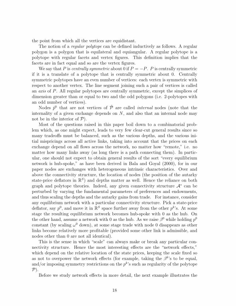
Example 3 (Strong equilibrium network effects in a hub-spoke network)Consider an architecture composed of one hub, 0, and three spokes, 1, 2 and 3. As-sume βk = β, all k ∈ K. Assume all autarky state-prices lie on a straight linesegment with p1 at one extremity, p0 in the middle equidistant between the extremi-ties, and p2 = p3 at the other extremity. We show that there are strong equilibriumnetwork effects. The intuition is straightforward: since µ0k is the same for all k 6= 0,the absence of strong network effects would amount to an arbitrageur distributionN0k = N/3, k = 1, 2, 3. But if that was true, then there would be 2N/3 arbitrageurspulling p0 into the direction p2 = p3 and only N/3 pulling it into the direction ofp1. Since only N/3 arbitrageurs are pulling pk, k = 1, 2, 3 towards the middle, inequilibrium the gains from trade between exchanges 0 and 1 are larger than between0 and either 2 or 3, violating the assumption that N0k = N/3. It is clear that theresults of this example still go through even if p0 is located closer to p1.

20

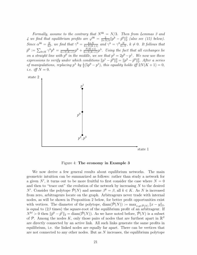
Formally, assume to the contrary that N0k = N/3. Then from Lemmas 3 and4 we find that equilibrium profits are ϕ0k = 2

2+N/3‖pk − p0‖2

2 (also see (15) below).

Since α0k = N6β

, we find that γ0 = 6+N6+N(K+1)

and γk = γ0 N6+N

, k 6= 0. It follows that

p0 :=∑

k∈K γkpk = 66+N(K+1)

p0 + N(K+1)6+N(K+1)

pλ. Using the fact that all exchanges lie

on a straight line with p0 in the middle, we see that p2 = 2p0−p1. We now use theseexpressions to verify under which conditions ‖p1 − p0‖2

2 = ‖p2 − p0‖22. After a series

of manipulations, replacing pλ by 14(5p0 − p1), this equality holds iff 2N(K + 1) = 0,

i.e. iff N = 0.

6

-state 1

state 2

t

t

t

p0

p1

p2, p3.

.

.

.

.

..

.

.

.

..

.

.

.

.

..

.

.

.

..

.

.

.

.

..

.

.

.

..

.

.

.

.

..

.

.

.

..

.

.

.

..

.

.

.

.

..

.

.

.

..

.

.

.

.

..

.

.

.

..

.

.

.

.

..

.

.

.

..

.

.

.

.

..

.

.

.

..

.

.

.

.

..

.

.

.

..

.

.

.

.

..

.

.

.

..

.

.

.

..

.

.

.

.

..

.

.

.

..

.

.

.

.

..

.

.

.

..

.

.

.

.

..

.

.

.

..

.

.

.

.

..

.

.

.

..

.

.

.

.

..

.

.

.

..

.

.

.

.

..

.

.

.

..

.

.

.

..

.

.

.

.

..

.

.

.

..

.

.

.

.

..

.

.

.

..

.

.

.

.

..

.

.

.

..

.

.

.

.

..

.

.

.

..

.

.

.

.

..

.

.

.

..

.

.

.

.

..

.

.

.

..

.

.

.

..

.

.

.

.

..

.

.

.

..

.

.

.

.

..

.

.

.

..

.

.

.

.

..

.

.

.

..

.

.

.

.

..

.

.

.

..

.

.

.

.

..

.

.

.

..

.

.

.

.

..

.

.

.

..

.

.

.

..

.

.

.

.

..

.

.

.

..

.

.

.

.

..

.

.

.

..

.

.

.

.

..

.

.

.

..

.

.

.

.

..

.

.

.

..

.

.

.

.

..

.

.

.

..

.

.

.

.

..

.

.

.

..

.

.

.

..

.

.

.

.

..

.

.

.

..

.

.

.

.

..

.

.

.

..

Figure 4: The economy in Example 3

We now derive a few general results about equilibrium networks. The maingeometric intuition can be summarized as follows: rather than study a network fora given N ′, it turns out to be more fruitful to first consider the case where N = 0and then to “trace out” the evolution of the network by increasing N to the desiredN ′. Consider the polytope P(N) and assume βk = β, all k ∈ K. As N is increasedfrom zero, arbitrageurs locate on the graph. Arbitrageurs never trade with internalnodes, as will be shown in Proposition 2 below, for better profit opportunities existwith vertices. The diameter of the polytope, diam(P(N)) := maxx,y∈P(N) ‖x − y‖2,is equal to (2β times) the square-root of the equilibrium profit of an arbitrageur. IfNkℓ > 0 then ‖pk − pℓ‖2 = diam(P(N)). As we have noted before, P(N) is a subsetof P. Among the nodes K, only those pairs of nodes that are furthest apart in R

S

are directly connected by an active link. All such links generate the same profits inequilibrium, i.e. the linked nodes are equally far apart. There can be vertices thatare not connected to any other nodes. But as N increases, the equilibrium polytope

21

contracts along those edges that are active, while the polytope remains centered inthe sense that pλ is always in the interior of P(N), pλ =

∑

k∈K λkpk(N), all N ≥ 0(see (28)). For N large enough this implies that hitherto inactive vertices becomeactive as the length of the active edges contracts to the length of the largest edgeemanating from the hitherto inactive vertex. At the same time, as the polytopecontracts, an internal node becomes itself a vertex for some N large enough, andat some yet higher N becomes an active node. This procedure is repeated until,as seen in Proposition 1, the polytope converges to the singleton point {pλ}. Weprovide some general results that provide the basis of our intuition, with finer pointsillustrated in particular examples later on.

Proposition 2 (Internal nodes) Suppose that A is either complete or hub-spokeand that βk = β, all k ∈ K. Then the equilibrium network (K,A∗) never involvestrade with an internal node unless A is hub-spoke with the internal node being thehub.

In particular, if the architecture is complete, the equilibrium network can never behub-spoke with an internal hub. It can, however, be hub-spoke with a vertex hub.For instance, assume that pk = p1, k = 1, . . . , K+1 and p0 6= p1. Then no arbitrageurchooses to arbitrage kℓ if k 6= 0 and ℓ 6= 0, and in equilibrium N0k = N/K, k 6= 0.

We call a polytope strongly symmetric if it is either a regular polytope, or acentrally symmetric polytope with equal axes. Of course, it can be both, e.g. thecube. Examples of non-regular polytopes that are centrally symmetric with equalaxes are the rectangle, the bipyramid (with equal axes) whose basis is a regular evenpolygon with six or more vertices,10 or any prism based upon an even regular polygon.A strongly symmetric polytope can be circumscribed by a sphere, so its center, asdefined above, always exists. In case the polytope is centrally symmetric, the centercoincides with its center of symmetry. We denote the family of strongly symmetricpolytopes by P

ss. Of all the polytopes, this family provides us with a clear intuitionas well as tractable closed-form solutions due to the symmetry between vertices.Intuitively it amounts to assuming that state prices are evenly distributed in statespace.

Proposition 3 (Strongly symmetric complete networks) Suppose that A is com-plete and that βk = β, all k ∈ K. Suppose further that there is an N ≥ 0, with equi-librium arbitrageur distribution {Nkℓ}, such that P(N) ∈ P

ss with no internal nodes.Then the center of P(N) is pλ, and the equilibrium network can be characterized asfollows, for all N ≥ N :

10A bipyramid is a pyramid pasted on both sides of the basis. Indeed we can take such a 3-bipyramid itself as the basis and construct a d-bipyramid, by repeatedly pasting s-dimensionalpyramids on both “sides” of the (s − 1)-dimensional pyramid. Provided we keep the axes equaleach time we increase the dimension, the result is a centrally symmetric polytope with equal axes.See Grunbaum (2003) for details.

22

i. If P(N) is a regular simplex, the equilibrium network is complete, with |A∗| =K(K + 1)/2.

ii. If P(N) is centrally symmetric with equal axes, the equilibrium network is notconnected for K > 1. It has K+1

2components, each consisting of two nodes

which are symmetric with respect to pλ.

iii. If P(N) is a regular odd polygon, the equilibrium network is a cycle: the neigh-bors of node k, k ∈ K, are the two vertices of the segment opposite to k. Also,|A∗| = K + 1.

In each case, P(N) belongs to the same family of polytopes as P(N), i.e. (i), (ii)or (iii), with the same center pλ, but with a smaller circumsphere. For N ≥ N ,A∗(N) = A∗(N), and

pk(N) = ν(N) pk(N) + (1 − ν(N)) pλ, (12)

Nkℓ(N) = [ν(N)]−1Nkℓ + b(N), kℓ ∈ A∗ (13)

Φ(N) = [ν(N)]2Φ(N), (14)

where ν(N) is strictly decreasing in N , with ν(N) = 1, ν(∞) = 0, and b(N) isstrictly increasing in N , with b(N) = 0, b(∞) = ∞. Moreover, Nkℓ(N) is an affinefunction of N .

Note that the cases (i)–(iii) in the proposition cover all possible regular polytopes.In addition, (ii) covers some non-regular polytopes as well. For the case in whichP(N) is a polygon with r vertices, with r odd and r ≥ 5, the equilibrium network isconnected but not complete (for r = 3 the polygon is in fact a simplex). The cycleshould obviously not be visualized as the polygon itself, since the neighbors of k arenot the adjacent nodes in the polytope but the ones that are maximally distant fromk.

We can specialize Proposition 3 to the case where N = 0, so that P is stronglysymmetric with vertex set {pk}k∈K . Then P(N) is a smaller strongly symmetricpolytope within the autarky polytope P, and P(N) contracts evenly to the sin-gleton {pλ} as N → ∞, with each state-price deflator pk converging on a straightline segment towards pλ, the center of the polytope. Equilibrium profits convergemonotonically to zero. Each active link attracts the same number of arbitrageurs.

For arbitrary polytopes convergence need not be along a linear trajectory but canbe along a nonlinear curve, either globally or piecewise. Examples will be given inthe sequel. However, even if P is not strongly symmetric, P(N) may be for some N .Interestingly, convergence is linear from that N onwards, with equilibrium numbersof arbitrageurs spread out according to the rules laid out in the proposition. Forinstance, suppose there are three exchanges and P is an isosceles triangle with thetwo sides that are equal making an angle greater than 60◦. Then the third side islonger and initially all arbitrageurs will concentrate on that link. As N increases,this side contracts, until the triangle becomes equilateral, i.e. a regular simplex. As

23

another example, reconsider Example 1. Here the autarky polytope is a rhombuswhich converges to a square. If we modify Example 1, so that the two lines in Figure2 do not cross at a right angle, then the autarky polytope is a parallelogram whichconverges to a rectangle. In both cases, there is an N for which the polytope P(N)is centrally symmetric with equal axes, so the proposition applies (in particular, part(ii)). In fact, this observation generalizes to all centrally symmetric polytopes:

Lemma 5 Suppose that A is complete and that βk = β, all k ∈ K. If P is centrallysymmetric, then there is an N such that P(N) is centrally symmetric with equal axes.

Arbitrageurs gravitate to the links that correspond to the longest axes of the poly-tope. This causes these axes to shorten until there is activity on all the axes. Thenthey must be equal.

If P(N) ∈ Pss with some internal nodes, the proposition still applies for N > N

as long as the nodes that are internal for P(N) are also internal for P(N). Let Nmax

be the maximum N for which this is the case and let C be the vertex set of P(N).Then we have linear convergence of pk to pλ

C , for N ∈ [N, Nmax], for all k ∈ C.In view of the importance of hub-spoke networks in delivering higher payoffs, it

is worth emphasizing the following corollary of Proposition 3:

Corollary 2 Suppose that A is complete and that βk = β, all k ∈ K. If P(N) ∈ Pss,

then the equilibrium network is not hub-spoke for any N ≥ N .

In particular if P is strongly symmetric with no internal nodes, then the equilibriumnetwork is not hub-spoke for any N . The intuition here is that if the architectureis complete and if equilibrium network is hub-spoke, then the autarky state-pricesmust be distributed “irregularly” or asymmetrically in R

S space, with some nodesfurther out (but with the mirror-nodes not also further out in a symmetrical fashion)or some other nodes in clusters.

The strong symmetry imposed in the previous proposition also implies that therecannot be strong network effects:

Corollary 3 (No strong network effects in Pss) Under the assumptions of Propo-

sition 3, there are no strong network effects.

Intuitively, strong network externalities imposed upon one node cannot emergein equilibrium because by symmetry those same externalities are also imposed onthe other relevant nodes. This causes them to mutually cancel each other out inequilibrium, and this is precisely what contributes to the relatively succinct closedform expressions. This does not say that there are no network externalities, ofcourse. For instance, in cases (i) and (iii) the state-prices and the state-contingentconsumptions on exchange k are affected by arbitrageur actions (and ultimately bypreferences and endowments of investors located) on any other exchange ℓ, no matterhow remote and indirectly connected.

24

7 Hub-Spoke Geometry

We now analyze the geometry of hub-spoke networks in a bit more detail. Arbitrageurprofits in an h0-architecture are easily calculated, using (9):

ϕ0k =βk + β0

[(1 +N0k)βk + β0]2· ‖pk − p0‖2

2 , (15)

with p0 given by (8). In equilibrium (with endogenous {N0k}) we must have ϕ0k =Φh0, for all k on which there is some arbitrage activity. The profit ϕ0k is a product oftwo terms. The first term is decreasing in βk, and therefore increasing in the depthof exchange k, while the second term captures the net gains from trade on exchangek, taking into account the fact that all other arbitrageurs, including those linking0 to j 6= k, also trade on 0 (hence p0 appears in lieu of p0). Consequently, there isa tradeoff between depth and equilibrium gains from trade. The following result isimmediate from an inspection of (15):

Proposition 4 (Equalizing differences: hub-spoke architecture) Suppose A =Ah0. Then:

i. Suppose N0k = N0ℓ > 0. ‖pk − p0‖22 > ‖pℓ − p0‖2

2 iff βk > βℓ.

ii. Suppose ‖pk − p0‖22 = ‖pℓ − p0‖2

2. Then N0k > N0ℓ iff βk < βℓ.

iii. Suppose βk = βℓ. Then N0k > N0ℓ iff ‖pk − p0‖22 > ‖pℓ − p0‖2

2.

Proposition 4 does not give us an explicit characterization of {N0k} since p0 itselfdepends on {N0k} in a complex manner. The symmetric case, however, is amenableto further analysis. We say that the nodes {pk}k∈K are symmetric with respect top0 if ‖pk − p0‖2 does not depend on k, for k 6= 0. Let L := aff({p0, pλ}). If p0 6= pλ,then L is the line passing through p0 and pλ; if p0 = pλ, then L is just the point pλ.We say that the nodes {pk}k∈K are symmetric with respect to L if for every k, thereis a pℓk , such that pℓk is the reflection of pk through L.

Proposition 5 (Symmetric hub-spoke networks) Suppose A = Ah0, and βk =β, all k ∈ K. Suppose further that the nodes {pk} are symmetric with respect to p0

and L. Then, p0(N) = ν(N)p0 + (1 − ν(N))pλ, where ν(N) is strictly decreasing inN , with ν(0) = 1 and ν(∞) = 0.

Suppose the above hypotheses hold except that the nodes {pk} are not necessar-ily symmetric with respect to p0. Then, p0(N) is in aff({p0, pλ}) and converges topλ. There is an array of exchanges {Ki}

ni=1 and arbitrageurs {Ni}

ni=1, with Ni >

Ni−1, p0 ∈ K1, Ki−1 ⊂ Ki, Kn = K, such that for N ∈ [Ni−1, Ni), p

0(N) ∈ν(Ni−1)p

0(Ni−1) + (1 − ν(Ni−1))pλKi

. We have ν(Ni−1) ∈ [0, 1], and for N ′ > N ≥Ni−1, ν(N

′) < ν(N).

25

Under the symmetry assumptions of the proposition, the equilibrium state-pricedeflator on the hub is pulled evenly “from both sides” and follows a linear trajectorytowards pλ. With symmetry with respect to both p0 and L, p0(N) converges to pλ

monotonically along the line segment joining p0 and pλ. If p0 = pλ, then in factp0(N) = pλ for all N . If symmetry fails and more nodes are one one side than onanother one (but with similar scale properties), then the trajectory is an arc benttowards the more plentiful, attracting, side.

Once p0(N) is determined, pk(N) is a convex combination of p0(N) and pk,

pk(N) = p0(N)+ 2N+2K

P

ℓ ‖pℓ−p0(N)‖2

‖pk−p0(N)‖2

(pk−p0(N)). When replacing p0(N) by ν(N)p0+

(1 − ν(N))pλ for instance we see that pk(N) converges to pλ on an arc turning itsconcavity towards p0.

Intuitively, assume N is initially zero. As N becomes positive, only the exchangesfurthest from p0 get connected. Those exchanges form K1. As N further increases,p0(N) monotonically tends towards pλ

K1:=∑

k∈K1

1K1

pk until N equals N1. N1 is thecritical number for which the new equilibrium gains from trade between 0 and anyof the exchanges in K1 equal those between 0 and one or more exchanges not in K1.Those exchanges when added to the ones in K1 form K2. As N further increases,p0(N) converges towards pλ

K2, and the argument can be repeated until Ki = Kn = K.

Whereas convergence on each segment [Ni, Ni−1) is monotonic, overall convergenceof p0 from p0 to pλ need not be monotonic because pλ

Kiis in the convex hull of p0

and pλKi−1

. This can be illustrated in a simple example:

Example 4 (Non-monotonicity in a hub-spoke network) Consider the h0 - ar-chitecture with four exchanges whose autarky state-prices lie on a straight line in R

S.By construction this architecture is symmetric with respect to L. p0 and p1 form theextremes of the polytope, with p2 = p3 assumed to be located in conv({p0, pλ

K1}),

K1 = {0, 1}. Since the gains from trade between p0 and p1 are largest, for smallenough N we have N01 = N . This will be true until N∗ which is so that p0(N∗)−p2 =p1(N∗)−p0(N∗) = 2[pλ

K1−p0(N∗)]. In other words, at N∗ all links will become active,

and for N > N∗, p0(N) converges to pλK . Solving for N∗ we get p0(N∗) = 2

3pλ

K1+ 1

3p2,

and it can be verified that pλK = 1

2pλ

K1+ 1

2p2. But pλ

K lies between p0(N∗) and p0, sofor N > N∗ p0(N) reverts back in the direction of p0 towards its limit pλ

K.

One can get further results by requiring yet more symmetry and assume thatautarky state prices form a polytope with the hub at the center:

Proposition 6 (Strongly symmetric networks with central hub) Suppose A =Ah0, β0 arbitrary, βk = β for all k = 1, . . . , K, and p0 = pλ. Suppose further thatP ∈ P

ss with no internal nodes other than node 0. Then the center of P is pλ. P(N)belongs to the same family of polytopes as P, with the same center pλ, but with asmaller circumsphere. We have

p0(N) = p0 = pλ (16)

26

6

-

state 1

state 2

s

p0

s

p0

s

p1

s

pλK1

s

p2, p3

s

pλ

s

p0(N∗)s

p1(N∗)

Figure 5: The economy in Example 4

and, for k 6= 0,

pk(N) =(β + β0)K

(β + β0)K + βNpk +

βN

(β + β0)K + βNpλ, (17)

N0k(N) =N

K, (18)

Φh0(N) =β + β0

[(1 +N/K)β + β0]2‖pk − p0‖2

2. (19)

Equilibrium profits given by (19) do not depend on k because p0 = pλ is the centerof P.11

When we consider vertex hubs we will adopt the convention of choosing exchange1 as the hub. This will be particularly useful when we compare central and vertexhubs later.

Proposition 7 (Simplex networks with vertex hub) Suppose A = Ah1, andβk = β for all k ∈ K. Suppose further that P is a regular simplex with no internalnodes. Then:

p1(N) =2K

N(K + 1) + 2Kp1 +

N(K + 1)

N(K + 1) + 2Kpλ (20)

11The only property of strongly symmetric polytopes that we use in the proof is that the circum-center (which is the center as we have defined it) and the centroid (which is the equally weightedconvex combination of the vertices) coincide. Hence Proposition 6 holds in fact for the larger familyof polytopes that have this property.

27

and, for k 6= 1,

pk(N) =2K

N + 2Kpk +

N

N + 2Kp1(N), (21)

N1k(N) =N

K, (22)

Φh1(N) =K3[N(N + 4)(K + 1) + 8K]

β(N + 2K)2[N(K + 1) + 2K]2‖pk − p1‖2

2. (23)

Φh1(N) is strictly decreasing in N . Furthermore,

‖pk(N) − p1(N)‖2 < ‖pk(N) − pℓ(N)‖2, for ℓ 6= 1, N > 0.

Equilibrium profits given by (23) do not depend on k because all the edges of aregular simplex are equal. Note that P(N) is not a regular simplex for N > 0.Nodes other than the hub are pulled closer to the hub than to other nodes.

The following proposition says roughly that for hub-spoke networks that are smallenough, network effects are absent. “Small” may be either in terms of N small, orK small, or in the sense that (λ0)−1 is small. The latter condition would apply forinstance if all investors have identical risk parameters βk,i, k ∈ K, and if the numberof investors on 0, I0, is large compared to the aggregate population. In that sensethe spokes are small compared to the hub.

Proposition 8 (No strong network effects in small hub-spoke networks)Suppose A = Ah0.

Assume that (i) βk = β for all k ∈ K and that N is small. Then there are nostrong equilibrium networks effects of type 2.

Alternatively, assume either that (ii) βk = β for all k = 1, . . . , K and λ0 is large,or alternatively that (iii) K = {0, 1, 2} with no further restrictions. Then there areno strong equilibrium network effects.

For hub-spoke networks with either large N or large K, examples can easily beconstructed where network effects matter. The foregoing discussions taken togetherfully characterize the case of three exchanges.

Example 5 (Three exchanges) Propositions 3 and 5 allow us to completely char-acterize the case K = {0, 1, 2}. This example also serves as an illustration for theprinciple that in order to understand a network for some given N ′, proposition 3 sug-gests that one fruitful alternative is to start N at zero and then raise N to N ′. Thatthe case with K = {0, 1, 2} is fully characterized follows from the observation thatone must be in either of the following three situations. Either only one link is active,say 01, in which case we know that equilibrium state prices lie on the segment betweenthe two autarky state-prices and they move on that segment towards the middle pointpλ. Unless p2 = pλ, at some point for larger N there will be trade with exchange 2.Assume without loss of generality that the active links are 01 and 02. Then we are

28

in a necessarily symmetric hub-spoke network. Then p0 converges linearly to pλ asN increases (and therefore also N01 and N02) while p1 and p2 converge towards pλ

along a parabola. Either N12 always stays at zero, or there might be a point where‖p0 − p1‖2 = ‖p0 − p2‖2 = ‖p1 − p2‖2, in which case Proposition 3 implies that allthree links become active and equilibrium state prices all converge linearly towardspλ.

8 Equilibrium vs Profit Maximizing Networks

In this section we study equilibrium networks further and contrast them to profitmaximizing networks.

Proposition 9 (Profits: central hub vs complete architecture) Suppose βk =β for all k 6= 0, and p0 = pλ. Suppose further that P ∈ P

ss with no internal nodes ex-cept for node 0. Then, provided β0 ≥ β, there is no activity on node 0 in the completearchitecture for any N . If β0 = β, then Φh0(N) > Φ(N), provided N > 2|A∗|, whereA∗ is the set of active links for the complete architecture. For arbitrary β0 > β, wehave Φh0(N) > Φ(N), provided N is sufficiently large.

Thus, if all exchanges have equal depth, the complete architecture is dominated aslong as there are at least two arbitrageurs on each active link. Moreover, the h0-architecture leads to higher payoffs for arbitrageurs no matter how illiquid it is, asmeasured by β0, provided there are sufficiently many arbitrageurs.

For the sake of intuition let us first focus on the case where P is centrally symmet-ric. Then the vertices come in pairs (k, ℓk) that are symmetrical with respect to pλ.Equilibrium profits are higher with a central hub. This is so even though the autarkygains from trade are higher on link kℓk than on the spokes of the h0-architecture (i.e.Φ(0) > Φh0(0)). The reason is the positive externality that arbitrageurs on spoke0k exert on arbitrageurs on the symmetrical spoke 0ℓk. Arbitrageurs on 0k pull p0

towards pk, thereby increasing ‖p0−pℓk‖2. Arbitrageurs on 0ℓk pull p0 in the oppositedirection, towards pℓk . Due to symmetry, the net impact on state prices on the hubis in fact zero, i.e. p0 = p0. The aggregate supply of both families of arbitrageurson the hub is also zero—any state-contingent consumption that is supplied to thehub by arbitrageurs on one spoke is absorbed by arbitrageurs on the other spoke.Thus the hub acts as a liquidity repository,12 channeling trades in such a mannerthat the two groups of arbitrageurs complement each other. The network-inducedcomplementarity is sufficient to compensate for the fact that the autarky gains from

12We do not define liquidity rigorously in this paper, which is left to a companion paper (Rahiand Zigrand (2007d)). Do notice however that the common measure of liquidity as depth (1/β0)does not do justice to exchange 0. If exchange 0 is the hub, it will attract a lot of trade with zeroequilibrium price impact, irrespective of β0. On the other hand, for any other architecture, there isno trade with exchange 0, even if 1/βk approaches infinity. It is purely the position in the networkwhich determines liquidity, rather than any of the standard metrics of liquidity in isolation.

29

trade between the center and any one of the extremes is considerably less than thegains from trade between the two extremes, ignoring the central exchange altogether.

The h0-architecture exhibits strategic complements. The more arbitrageurs on0k trade, the more profitable each trade becomes for the arbitrageurs on 0ℓk becauseon the one hand mispricings increase and on the other hand the arbitrageurs on link0k provide liquidity to the ones on 0ℓk and vice versa.

When the architecture is complete the market mechanism fails to achieve thisoutcome due to a Prisoner’s Dilemma. If arbitrageurs could agree to not trade onkℓk, they would be able to minimize price impact and increase profits. But, given theopportunity, each arbitrageur would rather arbitrage kℓk due to the much greatergains from trade. The result is a suboptimal arrangement with all arbitrageurs onkℓk.

13

For the case where P is not centrally symmetric, for example a simplex, essentiallythe same intuition applies. For each node k there is a facet that is opposite to it.The vertices of this facet pull p0 away from pk. Due to symmetry, the net impact onp0 is zero.

In fact the complete architecture is suboptimal for arbitrageurs even if there is nocentral exchange. The following proposition shows that a vertex hub delivers higherprofits as well. While a vertex of P is not central relative to the other vertices ofP, it gets pulled towards the center after some level of arbitrageur activity on thespokes.

Proposition 10 (Profits: central/vertex hub) Suppose K ≥ 3, βk = β for allk ∈ K, and p0 = pλ. Suppose further that P is a regular simplex with no internalnodes except for node 0. Then, for the complete and h1-architectures, there is noactivity on node 0 for any N . We have Φh0(N) > Φh1(N) > Φ(N), provided N ≥2K − 1.

Since node 0 is always isolated in the complete and h1-architectures, the ranking ofprofits in these architectures also holds if P has no internal nodes (replacing K byK + 1 in the proposition).

The reason why a vertex hub delivers higher profits is similar to the one given for acentral hub. If kℓ is left unarbitraged, there is less pressure for the prices on k and ℓ toconverge, leaving the arbitrages on 1k and 1ℓ more differentiated, and therefore moreprofitable. As N increases, equilibrium state-price deflators on k and ℓ converge topλ along an arc while p1 moves more quickly into the middle between pk and pℓ. Theeffect of this is again to induce strategic complements in that arbitrageurs provideliquidity to each other to some extent (but less than in the central hub case). It istherefore not hard to see that the distance between equilibrium state prices on k andℓ is high, so that if trade on kℓ was now allowed, some arbitrageurs would deviateto that link. Again a Prisoner’s Dilemma result obtains.

13Interestingly, even if arbitrageurs were allowed to arbitrage any number of links, they wouldonly arbitrage kℓk. Arbitrageurs facing the twin restrictions of not being able to trade on kℓk andof trading on only one link, are better off than completely unrestricted arbitrageurs.

30

Thus, for both the central and vertex hub-spoke architectures, the restrictionsimplicit in the architecture coordinate arbitrageur actions by pooling liquidity andby preventing Prisoner’s Dilemma type deviations. The state prices of the hub arein equilibrium (not necessarily in autarky) to some extent “in-between” the otherstate prices, therefore acting as a liquidity pool.

One way to interpret Propositions 9 and 10 is that profits are lower in the completearchitecture because convergence to the Walrasian state-price deflator pλ is faster.Let dk(N) and dk,hℓ(N) denote ‖pk(N) − pλ‖2

2 for the complete and hℓ-architecturesrespectively.

Proposition 11 (Speed of convergence: central hub vs complete architecture)Suppose βk = β for all k ∈ K, and p0 = pλ. Suppose further that P ∈ P

ss with nointernal nodes except for node 0. Then, for all N > 0,

d0(N) = d0,h0(N) = 0,

dk(N) < dk,h0(N), k 6= 0.

Also, dk(N) and dk,h0(N) are strictly decreasing in N for k 6= 0.

Proposition 12 (Speed of convergence: central/vertex hub) SupposeK ≥ 3,βk = β for all k ∈ K, and p0 = pλ. Suppose further that P is a regular simplex withno internal nodes except for node 0. Then, for all N > 0,

d0(N) = d0,h1(N) = d0,h0(N) = 0,

d1,h1(N) < d1(N) < d1,h0(N),

dk(N) < dk,h1(N) < dk,h0(N), k /∈ {0, 1}.

Also, the distance of each node k, k 6= 0, from pλ is strictly decreasing in N for allthree architectures.

Like Proposition 9, this result holds for the complete and h1-architectures even if Phas no internal nodes.

9 Networks and Social Welfare

In this section we analyze how the equilibrium utilities of investors depend on thearchitecture. Using investor (k, i)’s first order condition, we can write his utility (1)as:

Uk,i = ωk,i0 + 1⊤Πωk,i −

βk,i

2ωk,i⊤Πωk,i +

βk,i

2‖θk,i‖2

2.

Note that Uk,i depends on the asset structure only through the termW k,i := βk,i‖θk,i‖22.

We will find it convenient to refer to W k,i as the equilibrium utility of agent (k, i).From (2), we see that

θk,i =1

βk,i(pk,i − pk), k ∈ K.

31

Hence, we have

Lemma 6 (Equilibrium utilities) Given a network G∗, the equilibrium utility ofinvestor (k, i), k ∈ K, is

W k,i =1

βk,i‖pk,i − pk‖2

2.

An architecture is optimal for an investor if it results in the highest equilibriumutility for the investor among all possible architectures. An architecture is Paretooptimal for a group of agents if there is no alternative architecture that Paretodominates it in equilibrium for this group. An architecture is socially optimal if it isPareto optimal for the set of all agents, arbitrageurs and investors.

We say that investors on exchange k are homogeneous if they have the sameno-trade valuations, i.e. pk,i = pk, for all i ∈ Ik. We refer to an economy in whichinvestors are homogeneous within each exchange as a clientele economy. From thepoint of view of arbitrageurs, each clientele k ∈ K consists of agents with identicalcharacteristics.

We will focus now on a clientele economy. Lemma 6 gives us the following welfareindex for clientele k ∈ K:

W k :=∑

i∈Ik

W k,i =1

βk‖pk − pk‖2

2. (24)

We can think of W k as the inter-exchange gains from trade reaped by exchange kin moving from autarky to the arbitraged equilibrium. Note that W k = βk‖yk‖2

2,so that the gains from trade are proportional to the magnitude of state-contingentconsumption trading volume. In particular this implies that if there are only twoexchanges, the outcome of the game is Pareto optimal in view of the fact that yk =−yℓ. All the subtleties arise from network externalities across links.

In order to distinguish welfare across networks, we will reserve the notationW k forwelfare on exchange k in the complete architecture, and denote welfare on exchangek in the hℓ-architecture by W k,hℓ.

Proposition 13 (Welfare: central hub vs complete architecture) Suppose βk =β for all k ∈ K, and p0 = pλ. Suppose further that P ∈ P

ss with no internal nodesexcept for node 0. Then, for all N > 0,

W 0(N) = W 0,h0(N) = 0,

W k(N) > W k,h0(N), k 6= 0.

Also, W k(N) and W k,h0(N) are strictly increasing in N for k 6= 0.

Thus the complete architecture Pareto dominates the h0-architecture for investors.This is intuitive given our earlier result that, in the complete architecture, the state-price deflator on any exchange converges faster to the Walrasian state-price deflator(Proposition 11).

32

Proposition 14 (Welfare: central/vertex hub) Suppose K ≥ 3, βk = β for allk ∈ K, and p0 = pλ. Suppose further that P is a regular simplex with no internalnodes except for node 0. Then, for all N > 0,

W 0(N) = W 0,h1(N) = W 0,h0(N) = 0,

W 1,h1(N) > W 1(N) > W 1,h0(N),

W k(N) > W k,h1(N) > W k,h0(N), k /∈ {0, 1}.

Also, for k 6= 0, welfare is strictly increasing in N for all three architectures.

Like Propositions 9 and 12, this result holds for the complete and h1-architectureseven if P has no internal nodes.

When node 0 is the center of P, the interests of arbitrageurs and investors aredirectly opposed. Arbitrageurs benefit when the trades between exchanges k and ℓare “split” by having to pass through exchange 0, while agents on exchanges k andℓ appropriate these gains themselves when they are linked directly.

Investors on node 1 (a vertex of P) are better off if their exchange is the hubcompared to the complete architecture. The reason is that, if exchange 1 is the hub,the other exchanges cannot trade with each other directly. All trading must be routedthrough exchange 1. However, if the other nodes are arranged symmetrically aroundthe hub, as in the central hub case, the hub becomes just a conduit for liquidity, witharbitrageur trades on the hub being exactly offsetting. More generally, investors onthe hub are better off the more asymmetric the location of the spokes (see Rahi andZigrand (2007a) where we provide a complete analysis of the three-exchange case).

Such results cannot be obtained in the case where agents within an exchangeare heterogeneous. This is because, for a given pk, the deflator pk,i is essentiallyunrestricted, so any result that holds for the representative investor on exchange kcan be reversed for an individual agent on k.

10 Conclusion

*** To be written ***

33

A Appendix: Proofs

Proof of Lemma 1 Using (3), we can write the Lagrangian for arbitrageur n ∈Nkℓ as follows:

L =∑

m∈{k,ℓ}

[pm − βmym,nkℓ − βmym,\n]⊤Πym,n

kℓ − ψ⊤Π∑

m∈{k,ℓ}

ym,nkℓ ,

where ψ is the Lagrange multiplier vector attached to the no-default constraints, andcan be interpreted as a (shadow) state-price deflator of the arbitrageur. The firstorder conditions are:

pm − βmym,\n − 2βmym,nkℓ − ψ = 0, m ∈ {k, ℓ}

together with complementary slackness:

ψ ≥ 0,∑

m∈{k,ℓ}

ym,nkℓ ≤ 0, and ψ⊤

∑

m∈{k,ℓ}

ym,nkℓ

= 0. (25)

We can rewrite the first order conditions as follows:

pm − βmym,nkℓ − ψ = 0, m ∈ {k, ℓ}. (26)

It is easy to check that a solution to (25) and (26) is given by (5), with

ψ =

(

1

βk+

1

βℓ

)−1(1

βkpk +

1

βℓpℓ

)

. (27)

The Lagrange multiplier vector ψ is nonnegative if pk and pℓ are both nonnegative.This is indeed the case, as we will verify later (Lemma 2). The no-default constraintshold with equality. This argmax is in fact unique since the program is globallyconcave. Thus the CWE is symmetric, i.e. ym,n

kℓ does not depend on n.

Proof of Lemma 2 Consider a component C ∈ C. Then {pk}k∈C solves the system(7) restricted to C. Define the matrix m = [mkℓ]k,ℓ∈C by mkk := 1+βkαk and mkℓ :=−βkαkℓ for k 6= ℓ. Let M := m⊗IS×S. Then, letting p := {pk}k∈C and p := {pk}k∈C,(7) can be written as Mp = p. Noting the diagonal structure of each block of M ,we have |Mii| = 1 + βkαk, for some k, and

∑

j 6=i |Mij | =∑

ℓ 6=k | − βkαkℓ| = βkαk.Therefore, |Mii| >

∑

j 6=i |Mij |, i.e. M is strictly (row)diagonally dominant (and so ism).

We will appeal to the theory of M-matrices; see Berman and Plemmons (1979),henceforth BP. An M-matrix is a square matrix of the form sI − B, where B ≥ 0,and s ≥ rad(B), the spectral radius of B. These matrices also have the propertythat the diagonal elements are positive and the off-diagonal elements are nonpositive.By Theorem 6.2.3 in BP, both M and m are nonsingular M-matrices. Hence, there

34

exists a unique p solving Mp = p, namely p = M−1p. Since M−1 = (m−1 ⊗ IS×S),we can write pk = pη,k :=

∑

j∈C ηkjpj , where ηkj is element (k, j) of m−1. The

matrix m is irreducible, also called indecomposable (indeed it is irreducible if andonly if C is connected; see Theorem 2.2.7 in BP). Hence m−1 ≫ 0 by Theorem6.2.7 in BP, i.e. ηkj > 0, all k, j ∈ C. Since m1 = 1 we also have m−11 = 1,i.e.

∑

j∈C ηkj = 1, all k ∈ C. In other words, m−1 is a stochastic matrix. Finally,

from Theorem 2.5.12 in Horn and Johnson (1985), m−1 is strictly column diagonallydominant: ηjj >

∑

i6=j ηij.

Proof of Lemma 4 Using Lemma 1, the equilibrium profit of arbitrageur n ∈ Nkℓ

is

ϕkℓ = (qk − qℓ)⊤yk,nkℓ

= (pk − pℓ)⊤Πyk,nkℓ

=1

βk + βℓ· ‖pk − pℓ‖2

2.

Proof of Proposition 1 Let Φ(N) denote the equilibrium profit of an arbitrageurwhen the number of arbitrageurs is N . Then Φ(N) = 1

βk+βℓ‖pk(N) − pℓ(N)‖2

2, for

all kℓ ∈ A∗. We claim that Φ(∞) = 0. If not, there exists a constant c > 0such that Φ(N) > c for arbitrarily large N . Now limN→∞Nkℓ = ∞, for somekℓ ∈ A. Consider such a link kℓ. We have ‖pk(N) − pℓ(N)‖2

2 > (βk + βℓ)c, forarbitrarily large N,Nkℓ. Therefore, total arbitrageur supply on k by arbitrageurson kℓ, given by Nkℓyk,n

kℓ = Nkℓ

βk+βℓ [pk(N) − pℓ(N)], is unbounded: for any constant C,

howsoever large, there is an N and a state s for which this supply is greater than Cin absolute value. Suppose that the supply is in fact positive (if it is negative, thenwe can consider instead the state-s supply by arbitrageurs on kℓ to ℓ). Since pk ≥ 0,(4) implies that yk is bounded above. Due to (6), Nkk1yk,n

kk1must be unboundedly

negative in state s, for some k1. But then the state-s supply on exchange k1 byarbitrageurs active on kk1 is unboundedly positive, which places k1 in the samesituation as k was. Eventually the unboundedly large supply in state s must end upon some exchange km. If km 6= k, the condition that pkm ≥ 0 will be violated dueto (4). If km = k, consider the following sequence of inequalities that must hold:pk

s < pk1

s < pk2

s < . . . < pkms = pk

s , a contradiction. Basically, arbitrageurs cannotbe trading unboundedly large amounts without running afoul of the fact that atequilibrium agents are nonsatiated on every exchange.

Since Φ(N) → 0, and Φ(N) ≥ 1βk+βℓ‖p

k(N) − pℓ(N)‖22, for all kℓ ∈ A, we

must have pk(N) − pℓ(N) converging to zero, for all kℓ ∈ A. We claim that thisis in fact true for all k, ℓ ∈ K. For arbitrary k and ℓ, there is a path connectingthem, since G is connected, i.e. there is a sequence of distinct vertices {k1, . . . , kI}in K such that k1 = k, kI = ℓ and (ki, ki+1) ∈ A for all i = 1, . . . , I − 1. Now

35

‖pk(N) − pℓ(N)‖22 ≤

∑I−1i=1 ‖p

i(N) − pi+1(N)‖22. Since each of the terms in the sum

converges to zero, pk(N) − pℓ(N) converges to zero as well.Multiplying equation (7) by λk and summing over k ∈ K we get

∑

k∈K

λkpk(N) = pλ. (28)

Hence, for all k ∈ K,

‖pk(N) − pλ‖22 =

∥

∥

∥

∑

j∈K

λj[

pk(N) − pj(N)]

∥

∥

∥

2

2

≤∑

j∈K

λj‖pk(N) − pj(N)]‖22

where the inequality follows again from the triangle inequality followed by Jensen’sinequality. Since each term in the last sum converges to zero, pk(N) converges to pλ,for all k ∈ K.

Now consider C ∈ C(∞). Define N large enough so that for all N > N ,C(N) = C(∞). Multiplying equation (7) by λk

C and summing over k ∈ C we get, forall N > N ,

∑

k∈C

λkC p

k(N) = pλC .

Taking limits as N goes to infinity, we get pλC = pλ.

Proof of Proposition 2 Consider first the complete architecture and supposepj is internal. Then pj =

∑

k∈K∗ νkpk, where K∗ is a subset of the vertex set of

P, |K∗| ≥ 2, νk > 0 for all k, and∑

k∈K∗ νk = 1. For any ℓ ∈ K, we have

‖pj − pℓ‖22 =

∥

∥

∥

∑

k∈K∗

νk(pk − pℓ)∥

∥

∥

2

2

≤[

∑

k∈K∗

νk‖pk − pℓ‖2

]2

(29)

<∑

k∈K∗

νk‖pk − pℓ‖22 (30)

≤ maxk∈K∗

‖pk − pℓ‖22

where (29) follows from the triangle inequality and (30) from Jensen’s inequality.For a hub-spoke architecture the same argument goes through taking ℓ to be the

hub.

Proof of Proposition 3 Since βk = β, all k, (28) implies that

pλ =1

K + 1

∑

k∈K

pk(N), (31)

36

for all N . Moreover, since P(N) ∈ Pss with vertex set {pk(N)}k∈K , pλ is the center

of P(N).We see from (7) that equilibrium prices solve the following system of equations:

Λk := pk(N) − pk +1

2

∑

ℓ∈K

Nkℓ[pk(N) − pℓ(N)] = 0, k ∈ K. (32)

Using (12) and (13):

Λk = ν(N) pk(N) + (1 − ν(N)) pλ − pk +1

2

∑

ℓ∈K

Nkℓ[pk(N) − pℓ(N)]

+b(N)ν(N)

2

∑

ℓ∈Ck

[pk(N) − pℓ(N)], (33)

where Ck := {k} ∪ {ℓ | kℓ ∈ A∗} (note that the inclusion of k in Ck is just a matterof convenience, as the corresponding term of the sum is zero). Using (32) evaluatedat N = N , (33) simplifies to:

Λk = (1 − ν(N))[pλ − pk(N)] +b(N)ν(N)

2

∑

ℓ∈Ck

[pk(N) − pℓ(N)] (34)

If P(N) is a regular simplex, we claim that all links are active, so that |Ck| =K + 1. Using (31),

∑

ℓ∈Ck[pk(N) − pℓ(N)] = (K + 1)[pk(N) − pλ]. Now it is easy

to check that Λk = 0, for all k, for the following choice of ν(N) and b(N) (by directsubstitution into (34)):

ν(N) =K + N

N +K, b(N) =

2(N − N)

(K + 1)(K + N). (35)

It follows from (12) that ‖pk(N)− pℓ(N)‖22 = [ν(N)]2‖pk(N)− pℓ(N)‖2

2, which isindependent of kℓ due to the regularity of the simplex P(N). Therefore, profits areequalized across all links, with Φ(N) = [ν(N)]2Φ(N), and the network is complete,for all N ≥ N . Indeed, as N increases, all the edges of P(N) contract uniformly, sothat P(N) is a smaller K-simplex within P(N), with the same center pλ.

Now suppose P(N) is centrally symmetric with equal axes. For N = N , let ℓk bethe exchange whose equilibrium state-price deflator is centrally symmetric to that ofk, i.e. pℓ(N) = −pk(N) + 2pλ. We claim that, for ℓ 6= ℓk, N

kℓ = 0, for all N ≥ N .This implies that

∑

ℓ∈Ck[pk(N)− pℓ(N)] = pk(N)− pℓk(N) = 2(pk(N)− pλ). We can

verify that Λk = 0 for

ν(N) =K + 1 + 2N

K + 1 + 2N, b(N) =

2(N − N)

K + 1 + 2N.

Also, from (12), ‖pk(N) − pℓk(N)‖22 = [ν(N)]2‖pk(N) − pℓk(N)‖2

2, which is in-dependent of k since the axes of P(N) are equal. Therefore, profits are equalized

37

across all such links, which are K+12

in number. Clearly, given (12) and (13), P(N)will contract uniformly as N increases beyond N . So the same pairs of nodes willremain symmetric. It remains to show that links between non-symmetric nodes willbe inactive. If ℓ 6= ℓk,

‖pk(N) − pℓk(N)‖2 = ‖pk(N) − pλ‖2 + ‖pℓk(N) − pλ‖2 (36)

= ‖pk(N) − pλ‖2 + ‖pℓ(N) − pλ‖2 (37)

> ‖(pk(N) − pλ) + (pλ − pℓ(N))‖2 (38)

= ‖pk(N) − pℓ(N)‖2,

where (36) follows from the symmetry of k and ℓk with respect to the center pλ, (37)from the equality of the axes, and (38) from the triangle inequality, which is a strictinequality because pk(N) − pλ is not proportional to pℓ(N) − pλ. Hence Nkℓ = 0unless ℓ = ℓk.

Finally, suppose P(N) is a polygon with r vertices, r odd. Clearly, the nodesthat have maximal distance from k are the vertices of the segment that is oppositeto k. Let us denote these by ℓk and mk. Then we have

∑

ℓ∈Ck

[pk(N) − pℓ(N)] = 2

[

pk(N) −1

2[pℓk(N) + pmk(N)]

]

= 2[pk(N) − pλ][

1 + cos(π

r

)]

where the last equality follows from a simple trigonometric calculation (see Coxeter(1963), Fig. 1.1A). The values of ν(N) and b(N) for which Λk = 0 are:

ν(N) =K + 1 + N

[

1 + cos(

πr

)]

K + 1 +N[

1 + cos(

πr

)] , b(N) =N − N

K + 1 + N[

1 + cos(

πr

)] .

That the active links are as postulated is easily seen by the same argument as forthe previous two cases.

In all the three cases, it can be verified that∑

kℓ∈A∗ Nkℓ = [ν(N)]−1N+|A∗|b(N) =

N . |A∗| is K(K+1)2

for the simplex, K+12

for the centrally symmetric case, and K + 1for the odd polygon.

Proof of Lemma 5 Consider a link kℓk corresponding to an axis that is maximalin length (there can be many such axes). Clearly there is no activity on any of theshorter axes. We need to show that there is also no activity on any link mℓ thatdoes not correspond to an axis. A simple extension of the argument in the proof ofProposition 3 (equations (36)–(38)) gives us:

‖pk − pℓk‖2 = ‖pk − pλ‖2 + ‖pℓk − pλ‖2

≥ ‖pm − pλ‖2 + ‖pℓ − pλ‖2 (39)

> ‖(pm − pλ) + (pλ − pℓ)‖2 (40)

= ‖pm − pℓ‖2.

38

(39) holds as an equality only if both m and ℓ correspond to one end of an axis ofmaximal length. The inequality (40) is strict because m and ℓ are not the end pointsof an axis.

Proof of Proposition 5 Suppose the nodes {pk} are symmetric with respect toL. The reflection of pk through L is given by

pℓk = −pk + 2pλ + 2

⟨

pk − pλ,p0 − pλ

‖p0 − pλ‖22

⟩

(p0 − pλ), k ∈ K. (41)

Note that this formula holds for all k ∈ K (e.g. ℓ0 = 0), and also for the case wherep0 = pλ. For the moment we assume that γk(N) = γℓk(N). We will show later thatthis is implied by profit equalization across links. Multiplying both sides of (41) byγk and summing over k ∈ K, and using (8), we see that p0(N)−pλ = ν(N)(p0 −pλ),where

ν(N) =

⟨

p0(N) − pλ,p0 − pλ

‖p0 − pλ‖22

⟩

.

Hence p0(N) = ν(N)p0 + (1 − ν(N))pλ. Since p0(N) is equal to p0 at N = 0 andconverges to pλ as N goes to infinity, we have ν(0) = 1 and ν(∞) = 0. From (9),

pk(N) − p0(N) =2

2 +N0k(pk − p0(N)), k 6= 0. (42)

By profit equalization, 22+N0k ‖p

k − p0(N)‖2 does not depend on k, for k 6= 0, fromwhich we can deduce that

2 +N0k = (N + 2K)‖pk − p0(N)‖2

∑

ℓ≥1 ‖pℓ − p0(N)‖2

, k 6= 0. (43)

In particular N0k = N0ℓk , thus verifying that γk = γℓk .If we provisionally assume that ν(N) is continuous in N , then so is p0(N). This

in turn implies that {N0k} is continuous in N , and hence so is {γk}. Therefore ν(N)is continuous in N , verifying our provisional assumption.

We now establish monotonicity of ν. We argue by contradiction. Supposeν is not strictly monotone. Then as N increases, p0(N) crosses the same point pon the segment conv({p0, pλ}) more than once, i.e. there is an N ′ and N ′′, with0 ≤ N ′ < N ′′ <∞ such that p0(N ′) = p0(N ′′) = p. From (42) and (43),

pk(N) − p =2

N + 2K

∑

ℓ≥1 ‖pℓ − p‖2

‖pk − p‖2(pk − p); k 6= 1, N = N ′, N ′′.

Summing both sides over k ≥ 1 we get (using (31):

(K + 1)pλ − p−Kp =2

N + 2K

(

∑

ℓ≥1

‖pℓ − p‖2

)

∑

k≥1

pk − p

‖pk − p‖2, N = N ′, N ′′.

(44)

39

Notice that the LHS does not depend on N . Therefore we have

1

N ′ + 2K

∑

k≥1

pk − p

‖pk − p‖2

=1

N ′′ + 2K

∑

k≥1

pk − p

‖pk − p‖2

,

implying that∑

k≥1pk−p

‖pk−p‖2

= 0. But then p = pλ from (44). So if p 6= pλ, then

N = N ′, a contradiction. This establishes monotonicity.Now we remove the assumption of symmetry with respect to p0. Define K1 :=

{k ∈ K : ‖p0 − pk‖2 ≥ maxℓ∈K ‖p0 − pℓ‖2} ∪ {0} and pλK1

:= 1|K1|

∑

k∈K1pk. For the

set of nodes K1, ignoring all other nodes, the previous proof applies with the obviouschanges. In particular, symmetry with respect to L implies symmetry with respectto L1 := aff({p0, pλ

K1}) (indeed, L1 = L). Therefore p0(N) converges monotonically

to pλK1

as N → ∞. Now there will be a smallest N1 > 0 such that ‖pk(N1) −p0(N1)‖2 = ‖pℓ − p0(N1)‖2 for k ∈ K1 and ℓ 6∈ K1. Define K2 recursively as theunion of K1 with all nodes ℓ 6∈ K1 for which the previous condition applies, anddefine pλ

K2:= 1

|K2|

∑

k∈K2pk. A modification of the proof above again applies to the

world with nodes in K2 only. It can easily be seen that pλKi

is in the convex hull ofp0 and pλ

Ki−1. This argument is repeated until the finite Nn for which Kn = K.

Proof of Proposition 6 We have λ0 = 11+Kβ0/β

and λk = 1K+β/β0 . Using the fact

that p0 = pλ, this implies that pλ = 1K

∑

k≥1 pk. Therefore pλ is the center of P.

Plugging N0k = NK

into the γj weights in Lemma 3 we get γ0 = Kβ0+β(K+N)Kβ0(1+N)+β(K+N)

and γk = β0NKβ0(1+N)+β(K+N)

, k 6= 0, so that

p0(N) = γ0p0 + γ1Kpλ (45)

which is equal to pλ since p0 = pλ. Using (15),

Φh0(N) =β + β0

[(1 +N/K)β + β0]2‖pk − p0(N)‖2

2, (46)

from which (19) follows since p0(N) = p0. This expression does not depend on kbecause the pk’s are equidistant from the center p0 = pλ. The formula for pk(N) iseasy to check from (9).

Proof of Proposition 7 When N1k = NK

, (45) and (46) hold, with node 0 replacedby node 1. Hence (20) is verified, and

Φh1(N) =2

β

[

K

N + 2K

]2

‖pk − p1(N)‖22, (47)

Denoting the coefficient of p1 in (20) by ν(N), we have (suppressing the dependenceof p1 and ν on N):

‖pk − p1‖22 = ‖pk − p1 + (1 − ν)(p1 − pλ)‖2

2

= ‖pk − p1‖22 + (1 − ν)2‖p1 − pλ‖2

2 + 2(1 − ν)〈pk − p1, p1 − pλ〉. (48)

40

For vectors x, y and z in RS, we have

‖x− z‖22 = ‖x− y + y − z‖2

2

= ‖x− y‖22 + ‖y − z‖2

2 + 2〈x− y, y − z〉,

so that2〈x− y, y − z〉 = ‖x− z‖2

2 − ‖x− y‖22 − ‖y − z‖2

2. (49)

Using this to evaluate the inner product in (48), we get

‖pk − p1‖22 = (1 − ν)2‖p1 − pλ‖2

2 + ν‖pk − p1‖22 (50)

The (squared) ratio of the circumradius and the edge length of the simplex P is givenby a standard formula (see Coxeter (1963), p. 292–295):

‖pk − pλ‖22

‖pk − pℓ‖22

=K

2(K + 1), k, ℓ ∈ K. (51)

In particular, ‖p1 − pλ‖22 = K

2(K+1)‖pk − p1‖2

2. Substituting this, as well as the value

of ν, into (50), we get

‖pk − p1(N)‖22 =

K[N(N + 4)(K + 1) + 8K]

2[N(K + 1) + 2K]2‖pk − p1‖2

2 (52)

< ‖pk − p1‖22, ∀N > 0, (53)

where the inequality (53) holds because ‖pk − p1(N)‖22 is strictly decreasing in N

for all N ≥ 0 (this is easily verified from (52)). This also implies, from (47), thatΦh1(N) is strictly decreasing in N . The expression for profits (23) can be obtainedby substituting (52) into (46). The formula for pk(N), (21), follows from (9). Using(21) and (53), we have for N > 0 and ℓ 6= 1:

‖pk(N) − p1(N)‖2 =2K

N + 2K‖pk − p1(N)‖2

<2K

N + 2K‖pk − p1‖2

=2K

N + 2K‖pk − pℓ‖2

= ‖pk(N) − pℓ(N)‖2.

Proof of Proposition 8 Statement (i) can be seen as follows. Assume ‖pk−p0‖2 >‖pℓ − p0‖2. From Proposition 4 we know that N0k > N0ℓ iff ‖pk − p0(N)‖2 >‖pℓ − p0(N)‖2. Lemma 3 has shown that p0(N) can be made arbitrarily close to p0

by choosing N small enough, from which we can deduce that ‖pk −p0‖2 > ‖pℓ −p0‖2

implies for small N that ‖pk − p0(N)‖2 > ‖pℓ − p0(N)‖2 as well.

41

As to (ii), λ0 large is equivalent to β0 small relative to all other βk, k 6= 0. FromLemma 3 it follows again that p0(N) can be made arbitrarily close to p0 by choosingβ0 small enough, and Proposition 4 (iii) establishes the result.

Now to (iii), so suppose K = {0, 1, 2}. Let x = N01 and y = N02, and define

bk := β0

β0+βk , for k = 1, 2. Using (15), we find that

ϕ01(x, y) =[1 + (1 − b2)y][(1 + y)µ01 − b1yµ02] + y(1 + y)(b1 + b2 − 2b1b2)µ12

[1 +N + xy(1 − b1b2)]2,

ϕ02(x, y) =[1 + (1 − b1)x][(1 + x)µ02 − b2xµ01] + x(1 + x)(b1 + b2 − 2b1b2)µ12

[1 +N + xy(1 − b1b2)]2.

The equilibrium distribution of arbitrageurs (x, y) is given (ignoring integer con-straints) by the solution to ϕ01(x, y) = ϕ02(x, y), with x + y = N , a quadraticequation, provided a real solution exists and is an element of [0, N ]:

x2(1 − b1b2)(µ02 − µ01) + (2x−N)H + (N + 1)(µ02 − µ01) = 0, (54)

where

H := (N + 1)(1 − b2)µ01 + [1 − b1 −Nb1(1 − b2)]µ02 + (N + 1)(b1 + b2 − 2b1b2)µ12.

It can be verified that H > 0 unless µ01 = µ02 = µ12 = 0, in which case H = 0. Theresult follows: assume wlg that µ02 > µ01, then (54) implies that 2x − N < 0, i.e.N01 < N/2 < N02.

Proof of Proposition 9 For the complete architecture, p0 = pλ is the centerof P(N) for all N . In particular, it is internal for all N . Moreover β0 ≥ β. ByProposition 2, no trade occurs with exchange 0 and we can simply ignore it. FromProposition 3, equilibrium profits for the complete architecture are

Φ(N) = [ν(N)]2 Φ(0)

=1

2β[ν(N)]2‖pk − pℓ‖2

2, kℓ ∈ A∗

≤1

2β[ν(N)]2

[

‖pk − p0‖2 + ‖pℓ − p0‖2

]2, kℓ ∈ A∗ (55)

=2

β[ν(N)]2‖pk − p0‖2

2 (56)

where (55) follows from the triangle inequality ((55) holds as an equality if and onlyif the polytope P is centrally symmetric), and (56) from the centrality of p0.

For the h0-architecture, profits do depend on β0. Consider first the case of β0 = β.Comparing (56) with (19), and using the appropriate expression for ν(N) from theproof of Proposition 3 (recall that we are applying this proposition for K, not K+1,nodes), we see that Φ0(N) > Φ(N) if and only if N ≥ K(K−1) = 2|A∗| for the case

42

of the simplex, N > K = 2|A∗| for the centrally symmetric case, and N ≥ K

cos(πr )

for

the case of the odd polygon with r vertices. In the last case, the condition is moststringent for r = 3, i.e N ≥ 2K = 2|A∗|.

Now suppose β0 > β. It is immediate from (15) that N0k = NK

, so that

Φh0(N) =β + β0

[(

1 + NK

)

β + β0]2‖p

k − p0‖22

=K2(β + β0)

[K(β + β0) +Nβ]2‖pk − p0‖2

2. (57)

Comparing (56) and (57) for the case of the simplex, it suffices to show that, forsufficiently large N ,

K2(β + β0)

[K(β + β0) +Nβ]2>

2

β

[

K − 1

N +K − 1

]2

or[

N +K − 1

K(β + β0) +Nβ

]2

>2

β(β + β0)

[

K − 1

K

]2

.

This condition is satisfied for large N , since the limit of the LHS as N goes to infinityis 1

β2 . Cases (ii) and (iii) of Proposition 3 can be dealt with in analogous fashion,and we leave the details to the reader.

Proof of Proposition 10 For the complete architecture, there is no trade onnode 0 by Proposition 9. We claim the same is true for the h1-architecture. From(20),

p1(N) − pλ =2(K − 1)

NK + 2(K − 1)(p1 − pλ). (58)

Since p0 = pλ,

‖p1(N) − p0‖22 =

[

2(K − 1)

NK + 2(K − 1)

]2

‖p1 − p0‖22. (59)

Using (21), (52) and (51), in that order, we have for k /∈ {0, 1}:

‖p1(N) − pk(N)‖22 =

[

2(K − 1)

N + 2(K − 1)

]2

‖p1(N) − pk‖22

=2(K − 1)3[NK(N + 4) + 8(K − 1)]

[N + 2(K − 1)]2[NK + 2(K − 1)]2‖p1 − pk‖2

2

=4K(K − 1)2[NK(N + 4) + 8(K − 1)]

[N + 2(K − 1)]2[NK + 2(K − 1)]2‖p1 − p0‖2

2. (60)

It is easy to verify that (59) is strictly less than (60), i.e. node 0 will not see any tradein the h1-architecture. Therefore, for all computations concerning the complete and

43

h1-architectures, we can ignore node 0 and apply our results for these architecturesreplacing K by K − 1.

From (23) and (51), and the fact that p0 = pλ,

Φh1(N) =(K − 1)3[NK(N + 4) + 8(K − 1)]

β[N + 2(K − 1)]2[NK + 2(K − 1)]2‖pk − p1‖2

2 (61)

=2K(K − 1)2[NK(N + 4) + 8(K − 1)]

β[N + 2(K − 1)]2[NK + 2(K − 1)]2‖pk − p0‖2

2. (62)

Comparing (62) with (19), Φh0(N) > Φh1(N) if and only if

K[N + 2(K − 1)]2[NK + 2(K − 1)]2 > (K − 1)2(N + 2K)2[NK(N + 4) + 8(K − 1)].

After some laborious (but straightforward) algebraic manipulations, this conditioncan be rewritten as:

1

9

[

4K(K2 − 9)(N3 + 8K) + 3NK(K − 3)(N3 + 20N + 64K) + 144K(N + 1)

+ 12N(7NK2 + 6N + 44K3) +K2(7N4 − 144K3 + 256K2)

+N2K2(5N2 − 36K) + 32NK3(N2 − 8K) +NK2(3N3 − 32K2)]

> 0,

which is satisfied for K ≥ 3 and N ≥ 2K − 1 (all the bracketed terms are nonnega-tive).

For the complete architecture, using (14) and (35), with K − 1 instead of K:

Φ(N) =1

2β

[

K − 1

N +K − 1

]2

‖pk − p1‖22.

Comparing with (61), Φh1(N) > Φ(N) if and only if

2(K − 1)[NK(N + 4) + 8(K − 1)]

[N + 2(K − 1)]2[NK + 2(K − 1)]2>

1

(N +K − 1)2.

After some tedious algebra it can be shown that this condition is equivalent to (sinceK ≥ 3)

N3K − 2N(K − 1)2(K + 3) − 8(K − 1)3 > 0.

It is easy to check that this condition is satisfied if N ≥ 2K − 1. In fact, the weakercondition N ≥ 2(K − 1) suffices for K ≥ 5.

Proof of Proposition 11 Using (12) and (17):

dk(N) = [ν(N)]2‖pk − pλ‖22, k ∈ K, (63)

dk,h0(N) =

[

2K

N + 2K

]2

‖pk − pλ‖22, k ∈ K. (64)

44

These equations hold trivially for k = 0 since p0 = p0 = pλ. In the complete archi-tecture there is no activity on node 0 (Proposition 10), while in the h0-architecturethe equilibrium price is equal to p0 for all N due to offsetting trades with the othernodes (Proposition 6). It is easy to check that

ν(N) <2K

N + 2K(65)

in all the three cases studied in Proposition 3 (as in the proof of Proposition 9, weapply Proposition 3 for K nodes, not K + 1). The result follows.

Proof of Proposition 12 For the complete and h1-architectures, there is noactivity on node 0 (Proposition 10). So we apply our results for these architecturesfor K − 1 instead of K. The result for exchange 0 follows as in Proposition 11.

Consider the h1-architecture. From (58),

d1,h1(N) =

[

2(K − 1)

NK + 2(K − 1)

]2

‖p1 − pλ‖22. (66)

For k /∈ {0, 1},

pk(N) − pλ =2(K − 1)

N + 2(K − 1)(pk − pλ) +

N

N + 2(K − 1)[p1(N) − pλ]

=2(K − 1)

N + 2(K − 1)

[

(pk − pλ) +N

NK + 2(K − 1)(p1 − pλ)

]

from (21) and (58). Therefore,

dk,h1(N) =

[

2(K − 1)

N + 2(K − 1)

]2[

‖pk − pλ‖22 +

(

N

NK + 2(K − 1)

)2

‖p1 − pλ‖22

+

(

2N

NK + 2(K − 1)

)

〈pk − pλ, p1 − pλ〉

]

, k /∈ {0, 1}. (67)

Using (49) and (51), and the fact that all vertices of P are equidistant from pλ, wesee that 〈pk − pλ, pλ − p1〉 = 1

K−1‖pk − pλ‖2

2. Substituting into (67), some algebraicmanipulations give us:

dk,h1(N) =4(K − 1)2

(

[NK + 2(K − 1)]2 −N(N + 4))

[N + 2(K − 1)]2[NK + 2(K − 1)]2‖pk − pλ‖2

2, k /∈ {0, 1}.

(68)From (63) and (35),

dk(N) =

[

K − 1

N +K − 1

]2

‖pk − pλ‖22, k ∈ K. (69)

45

The ranking for exchange 1 follows from (64), (66) and (69). Comparing (68)with (69), we see after some tedious algebra that dk(N) < dk,h1(N) for all N > 0,since K ≥ 3. Finally, dk,h1(N) < dk,h0(N), for N > 0, follows from (64) and (68).

Monotonicity with respect to N can be deduced from the relevant expressions(64), (66), (68) and (69).

Proof of Proposition 13 The welfare index of clientele k ∈ K is given by (24).Using (12) and (17):

W k(N) =1

β[1 − ν(N)]2‖pk − pλ‖2

2, k ∈ K, (70)

W k,h0(N) =1

β

[

N

N + 2K

]2

‖pk − pλ‖22, k ∈ K. (71)

Now the result follows from (65).

Proof of Proposition 14 The result for exchange 0 follows from the correspond-ing result in Proposition 12. From (20),

W 1,h1(N) =1

β

[

NK

NK + 2(K − 1)

]2

‖p1 − pλ‖22.

For k /∈ {0, 1}, we use (21), (52) and (51), in that order, to get

W k,h1(N) =1

β

[

N

N + 2(K − 1)

]2

‖pk − p1(N)‖22 (72)

=1

β·N2(K − 1)[NK(N + 4) + 8(K − 1)]

2[N + 2(K − 1)]2[NK + 2(K − 1)]2‖pk − p1‖2

2

=1

β·

N2K[NK(N + 4) + 8(K − 1)]

[N + 2(K − 1)]2[NK + 2(K − 1)]2‖pk − pλ‖2

2, k /∈ {0, 1}.

(73)

From (70) and (35),

W k(N) =1

β

[

N

N +K − 1

]2

‖pk − pλ‖22, k ∈ K. (74)

We now compare (71), (73) and (74). It is easy to check W 1,h1(N) > W 1(N) >W 1,h0(N). A tedious computation also verifies that W k(N) > W k,h1(N) for k /∈{0, 1}. Also for k /∈ {0, 1}, W k,h1(N) > W k,h0(N) provided

K[NK(N + 4) + 8(K − 1)] ≥ [NK + 2(K − 1)]2,

a condition that is easily verified.Monotonicity of welfare with respect to N is straightforward to check (for the case

of W k,h1(N) it follows from (72) and the observation made in the proof of Proposition7 that ‖pk − p1(N)‖2

2 is decreasing in N).

46

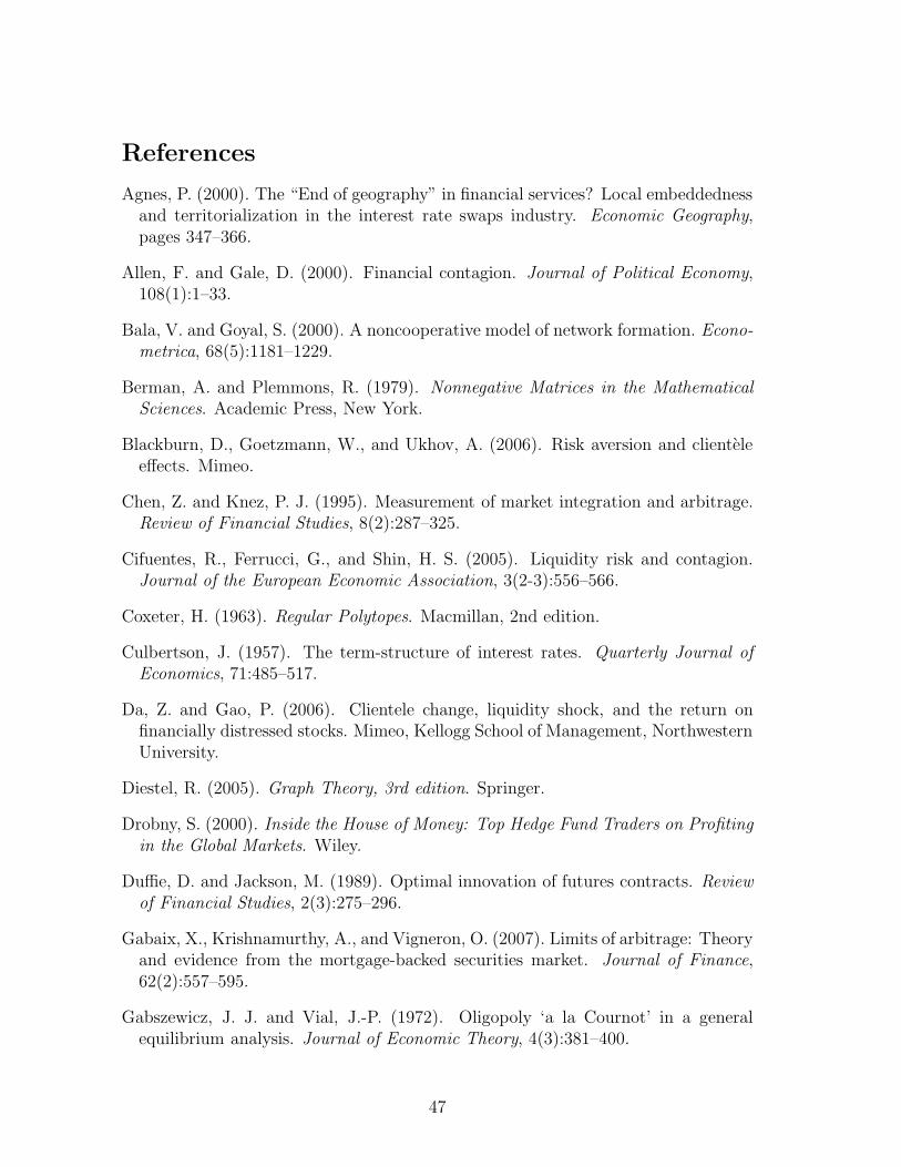
References

Agnes, P. (2000). The “End of geography” in financial services? Local embeddednessand territorialization in the interest rate swaps industry. Economic Geography,pages 347–366.

Allen, F. and Gale, D. (2000). Financial contagion. Journal of Political Economy,108(1):1–33.

Bala, V. and Goyal, S. (2000). A noncooperative model of network formation. Econo-metrica, 68(5):1181–1229.

Berman, A. and Plemmons, R. (1979). Nonnegative Matrices in the MathematicalSciences. Academic Press, New York.

Blackburn, D., Goetzmann, W., and Ukhov, A. (2006). Risk aversion and clienteleeffects. Mimeo.

Chen, Z. and Knez, P. J. (1995). Measurement of market integration and arbitrage.Review of Financial Studies, 8(2):287–325.

Cifuentes, R., Ferrucci, G., and Shin, H. S. (2005). Liquidity risk and contagion.Journal of the European Economic Association, 3(2-3):556–566.

Coxeter, H. (1963). Regular Polytopes. Macmillan, 2nd edition.

Culbertson, J. (1957). The term-structure of interest rates. Quarterly Journal ofEconomics, 71:485–517.

Da, Z. and Gao, P. (2006). Clientele change, liquidity shock, and the return onfinancially distressed stocks. Mimeo, Kellogg School of Management, NorthwesternUniversity.

Diestel, R. (2005). Graph Theory, 3rd edition. Springer.

Drobny, S. (2000). Inside the House of Money: Top Hedge Fund Traders on Profitingin the Global Markets. Wiley.

Duffie, D. and Jackson, M. (1989). Optimal innovation of futures contracts. Reviewof Financial Studies, 2(3):275–296.

Gabaix, X., Krishnamurthy, A., and Vigneron, O. (2007). Limits of arbitrage: Theoryand evidence from the mortgage-backed securities market. Journal of Finance,62(2):557–595.

Gabszewicz, J. J. and Vial, J.-P. (1972). Oligopoly ‘a la Cournot’ in a generalequilibrium analysis. Journal of Economic Theory, 4(3):381–400.

47

Galeotti, A., Goyal, S., Jackson, M. O., Vega-Redondo, F., and Yariv, L. (2006).Network games. Mimeo, University of Essex and Caltech.

Goyal, S. and Joshi, S. (2005). Unequal connections. Mimeo, University of Essex.

Grunbaum, B. (2003). Convex Polytopes. Springer-Verlag, 2nd edition.

Horn, R. and Johnson, C. (1985). Matrix Analysis. Cambridge University Press.

Lewis, K. (1999). Trying to explain home bias in equities and consumption. Journalof Economic Literature, 37(2):571–608.

Mas-Colell, A. (1982). The Cournotian foundations of Walrasian equilibrium theory:an exposition of recent theory. In Hildenbrand, W., editor, Advances in EconomicTheory. Cambridge University Press.

Massa, M., Peyer, U., and Tong, Z. (2005). Limits of arbitrage and corporate financialpolicy. CEPR Discussion Paper, No. 4829.

Modigliani, F. and Sutch, R. (1966). Innovations in interest rate policy. AmericanEconomic Review, 56(2):178–197.

Rahi, R. and Zigrand, J.-P. (2007a). Arbitrage networks: The three-exchange case.Mimeo, London School of Economics.

Rahi, R. and Zigrand, J.-P. (2007b). Financial innovation in arbitrage networks.Mimeo, London School of Economics.

Rahi, R. and Zigrand, J.-P. (2007c). Strategic financial innovation in segmentedmarkets. Review of Financial Studies. Forthcoming.

Rahi, R. and Zigrand, J.-P. (2007d). A theory of strategic intermediation and en-dogenous liquidity. Mimeo, London School of Economics.

48