Robustness for 2D Symmetric Tensor Field Topologybeiwang/publications/Tensor_Field_Robustness... ·...
25
Robustness for 2D Symmetric Tensor Field Topology Bei Wang and Ingrid Hotz Abstract Topological feature analysis is a powerful instrument to understand the essential structure of a dataset. For such an instrument to be useful in applications, however, it is important to provide some importance measure for the extracted fea- tures that copes with the high feature density and discriminates spurious from impor- tant structures. Although such measures have been developed for scalar and vector fields, similar concepts are scarce, if not nonexistent, for tensor fields. In particular, the notion of robustness has been proven to successfully quantify the stability of topological features in scalar and vector fields. Intuitively, robustness measures the minimum amount of perturbation to the field that is necessary to cancel its critical points. This chapter provides a mathematical foundation for the construction of a fea- ture hierarchy for 2D symmetric tensor field topology by extending the concept of robustness, which paves new ways for feature tracking and feature simplification of tensor field data. One essential ingredient is the choice of an appropriate metric to measure the perturbation of tensor fields. Such a metric must be well-aligned with the concept of robustness while still providing some meaningful physical interpre- tation. A second important ingredient is the index of a degenerate point of tensor fields, which is revisited and reformulated rigorously in the language of degree the- ory. 1 Introduction As a linear approximation of physical phenomena, tensors play an important role in numerous engineering, physics, and medical applications. Examples include various Bei Wang University of Utah, Salt Lake City, USA, e-mail: [email protected] Ingrid Hotz Link¨ oping University, Norrk¨ oping, Sweden, e-mail: [email protected] 1
Transcript of Robustness for 2D Symmetric Tensor Field Topologybeiwang/publications/Tensor_Field_Robustness... ·...
Robustness for 2D Symmetric Tensor FieldTopology
Bei Wang and Ingrid Hotz
Abstract Topological feature analysis is a powerful instrument to understand theessential structure of a dataset. For such an instrument to be useful in applications,however, it is important to provide some importance measure for the extracted fea-tures that copes with the high feature density and discriminates spurious from impor-tant structures. Although such measures have been developed for scalar and vectorfields, similar concepts are scarce, if not nonexistent, for tensor fields. In particular,the notion of robustness has been proven to successfully quantify the stability oftopological features in scalar and vector fields. Intuitively, robustness measures theminimum amount of perturbation to the field that is necessary to cancel its criticalpoints.
This chapter provides a mathematical foundation for the construction of a fea-ture hierarchy for 2D symmetric tensor field topology by extending the concept ofrobustness, which paves new ways for feature tracking and feature simplification oftensor field data. One essential ingredient is the choice of an appropriate metric tomeasure the perturbation of tensor fields. Such a metric must be well-aligned withthe concept of robustness while still providing some meaningful physical interpre-tation. A second important ingredient is the index of a degenerate point of tensorfields, which is revisited and reformulated rigorously in the language of degree the-ory.
1 Introduction
As a linear approximation of physical phenomena, tensors play an important role innumerous engineering, physics, and medical applications. Examples include various
Bei WangUniversity of Utah, Salt Lake City, USA, e-mail: [email protected]
Ingrid HotzLinkoping University, Norrkoping, Sweden, e-mail: [email protected]
1
2 Bei Wang and Ingrid Hotz
descriptors of stress at a point in a continuous medium under load or the diffusioncharacteristics of water molecules in fibrous media. Tensors provide a powerful andsimple language to describe anisotropic phenomena for which scalars and vectorsare not sufficient, but the analysis of tensor fields is a complex and challenging task.Therefore, visualization becomes a crucial capability to support the understandingof tensor fields. See [18] for a survey on the analysis and visualization of second-order tensors.
In this chapter, we are especially interested in a structural characterization ofsymmetric second-order tensor fields using topological methods, which can formthe basis of advanced analysis and visualization methods. Roughly speaking, ten-sor field topology segments the tensor field into regions of equivalent tensor linebehavior. Conceptually, it is closely related to the vector field topology. Degeneratepoints in tensor fields take the role of critical points in vector fields, and tensor linescorrespond to streamlines. However, despite these parallels, there are also many dif-ferences.
First, whereas critical points in vector fields behave as sources and sinks andseparatrices can be interpreted as material boundaries of flows, the topological fea-tures of tensor fields often do not have a direct physical meaning. Degenerate pointsare points of high symmetry with isotropic behavior and thus might be consideredas being especially boring. However, they play an important role from a structuralpoint of view, as they are points where the eigenvector field is not uniquely specifiedand thus not necessarily continuous.
Second, there are also major structural differences in comparison to vector fields,because eigenvector fields have no specified orientation. In the 2D case, they exhibita rotational symmetry with a rotational angle of π . As such, they are a special caseof N-symmetric direction fields [17], which are important for many applications ingeometry processing and texture design. For example, the eigenvector fields of thecurvature tensor have been used for the purpose of quadrangular re-meshing, wheredegenerate points are mesh vertices with distinct valency [1, 16]. A related applica-tion is the synthesis of textures, for example, by defining the stroke directions as aneigenvector field of some tensor field, where degenerated points account for pointswith non-trivial texture characteristics [30, 3]. For both applications, it is essential tohave control over the number of degenerate points. Furthermore, in tensor field anal-ysis, it can also be beneficial to have control over not only the degenerated points butalso their cancellation for feature-preserving interpolation and smoothing [15, 24].
While tensor field topology has attracted the most attention in geometric applica-tions, it was introduced along with the vector field topology in visualization appli-cations by Delmarcelle [9] and Tricoche [26]. Since the introduction of tensor fieldtopology, theoretical and application-driven advancement has been slow for severalreasons (in contrast to vector field topology): the lack of theory for 3D tensor fields,the complexity of the resulting topological structures, and the challenge of a directinterpretation of such structures in the application domain. However, there has beensome recent, encouraging effort by Zhang et al. [31] concerning a theory for 3D ten-sor field and the application of stress tensor field analysis. To further develop tensorfield topology as a useful analysis tool, we are convinced that a major requirement is
Robustness for 2D Symmetric Tensor Field Topology 3
to find a mathematically rigorous way to cope with the high density of the extractedtopological features, even in the setting of 2D tensor fields, where a large number ofstructures originate from extended isotropic regions and are very sensitive to smallchanges in the data.
The most important requirement in applications is a stable topological skeletonrepresenting the core structure of the data. For all the above-mentioned applications,tensor field topology can provide a means for the controlled manipulation and sim-plification of data. In this work, we introduce a measure for the stability of degener-ate points with respect to small perturbations of the field. The measure is based onthe notion of robustness and well group theory, which has already been successfullyapplied to vector fields. We extend this concept to 2D symmetric second-order ten-sor fields to lay the foundation for a discriminative analysis of essential and spuriousfeatures.
The work presented in this chapter paves the way for a complete framework oftensor field simplification based on robustness. We generalize the theory of robust-ness to the space of analytical tensor fields. In particular, we discuss the appropriatemetrics for measuring the perturbations of tensor fields, but a few challenges remain.First, we need to develop efficient and stable algorithms to generate a hierarchicalscheme among degenerate points. Second, the actual simplification of the tensorfield using the hierarchical representation and cancellation of degenerate points istechnically non-trivial. In this chapter, we focus on the first part by providing thenecessary foundation for the following steps.
Our main contributions are threefold: First, we interpret the notion of tensor in-dex under the setting of degree theory; Second, we define tensor field perturbationsand make precise connections between such perturbations with the perturbations ofbidirectional vector fields; Third, we generalize the notion of robustness to the studyof tensor field topology.
This chapter is structured as follows: After reviewing relevant work in Section 2,we provide a brief description of well group theory and robustness for vector fieldsin Section 3. Then in Section 4, we reformulate some technical background in ten-sor field topology in a way that is compatible with robustness, by introducing thebidirectional vector field and an anisotropy vector field. The anisotropy vector fieldthen provides the basis for Section 5 in which the notion of robustness is extendedto the tensor field setting.
2 Related work
Tensor Field Topology. Previous research has examined the extraction, simplifi-cation, and visualization of the topology of symmetric second order tensor fieldson which this work builds. The introduction of topological methods to the struc-tural analysis of tensor fields goes back to Delmarcelle [9]. In correspondence tovector field topology, Delmarcelle has defined a topological skeleton, consisting ofdegenerate points and separatrices, which are tensor lines connecting the degenerate
4 Bei Wang and Ingrid Hotz
points. Delmarcelle has mainly been concerned with the characterization of degen-erate points in two-dimensional fields. Therefore he also provided a definition forthe index of a critical point. Tricoche et al. [27] built on these ideas by develop-ing algorithms to apply the concept of topological skeleton to real data. A centralquestion of their work is the simplification of the tensor field topology and track-ing it over time. They succeeded in simplifying the field, but the algorithm containsmany parameters and is very complex. A robust extraction and classification algo-rithm for degenerate points has been presented by Hotz et al. [15]. Their methodis based on edge labeling using an eigenvector-based interpolation. This work hasbeen extended by Auer et al. [2] to cope with the challenge of discontinuities oftensor fields on triangulated surfaces. While the characteristics of the tensor fieldtopology for two-dimensional fields are similar to the vector field topology, it is ingeneral not possible to define a global vector field with the same topological struc-ture. It is possible, however, to define a vector field whose critical points are locatedin the same positions as the degenerate points of the tensor field by duplicating theirindexes. This idea has been used by Zhang et al. [30] for constructing a simplifiedtensor field for texture generation. Our method follows a similar line of thought butgoes a step further by defining an isometric mapping of the tensor field to a vectorfield.
Robustness for Vector Fields. In terms of vector field topology, topological meth-ods have been employed extensively to extract features such as critical points andseparatrices for vector field visualization [19] and simplification [8]. Motivated byhierarchical simplification of vector fields, the topological notion of robustness hasbeen used to rank the critical points by measures of their stability. Robustness isclosely related to the notion of persistence [10]. Introduced via the algebraic con-cept of well diagram and well group theory [11, 12, 7], it quantifies the stabilityof critical points with respect to the minimum amount of perturbation in the fieldsrequired to remove them. Robustness has been shown to be very useful for the anal-ysis and visualization of 2D and 3D vector fields [28, 23]. In particular, it is the coreconcept behind simplifying a 2D vector field with a hierarchical scheme that is inde-pendent of the topological skeleton [22]; and it leads to the first ever 3D vector fieldsimplification, based on critical point cancellation [20]. Measures of robustness alsolead to a fresh interpretation of critical point tracking [21]: Stable critical points canbe tracked more easily and more accurately in the time-varying setting.
In this paper, we extend the notion of robustness to the study of tensor fieldtopology. We would like to rely on such a notion to develop novel, scalable, andmathematically rigorous ways to understand tensor field data, especially questionspertaining to their structural stability. We believe that robustness holds the key toincrease the interpretability of tensor field data, and may lead to a new line of re-search that spans feature extraction, feature tracking, and feature simplification oftensor fields.
Robustness for 2D Symmetric Tensor Field Topology 5
3 Preliminaries on Robustness for Vector Fields
In this section, we briefly review the relevant technical background of robustnessfor 2D vector field such as critical points, degrees, indices, well groups and welldiagrams. These concepts are important for developing and understanding the ex-tensions of robustness for the tensor field.
Critical Point and Sublevel Set. Let f : R2→ R2 be a continuous vector field. Acritical point of f is a zero of the field, i.e., f (x) = 0. Define f0 : R2 → R as thevector magnitude of f , f0(x) = || f (x)||2, for all x ∈ R2. Let Fr denote the sublevelset of f0, Fr = f−1
0 (−∞,r], that is, all points in the domain with a magnitude up tor. In particular, F0 = f−1(0) is the set of critical points. A value r > 0 is a regularvalue of f0 if Fr is a 2-manifold, and for all sufficiently small ε > 0, f−1
0 [r−ε,r+ε]
retracts to f−10 (r); otherwise it is a critical value. We assume that f0 has a finite
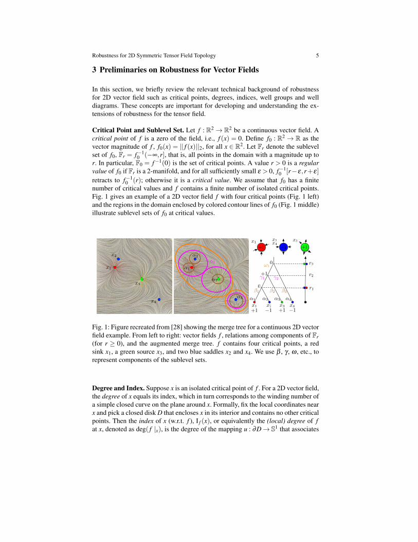
number of critical values and f contains a finite number of isolated critical points.Fig. 1 gives an example of a 2D vector field f with four critical points (Fig. 1 left)and the regions in the domain enclosed by colored contour lines of f0 (Fig. 1 middle)illustrate sublevel sets of f0 at critical values.
x1
x2
x3
x4
1
2
3
1
2
!1
x2x1x3
1+1 +1x4
1 32
21
!1
r2
r1
r3
x1 x2 x3 x4+1 1 +1 1
0
+1
0↵1
↵2
↵3
↵4 ↵1 ↵2 ↵3 ↵4
Fig. 1: Figure recreated from [28] showing the merge tree for a continuous 2D vectorfield example. From left to right: vector fields f , relations among components of Fr(for r ≥ 0), and the augmented merge tree. f contains four critical points, a redsink x1, a green source x3, and two blue saddles x2 and x4. We use β , γ , ω , etc., torepresent components of the sublevel sets.
Degree and Index. Suppose x is an isolated critical point of f . For a 2D vector field,the degree of x equals its index, which in turn corresponds to the winding number ofa simple closed curve on the plane around x. Formally, fix the local coordinates nearx and pick a closed disk D that encloses x in its interior and contains no other criticalpoints. Then the index of x (w.r.t. f ), I f (x), or equivalently the (local) degree of fat x, denoted as deg( f |x), is the degree of the mapping u : ∂D→ S1 that associates
6 Bei Wang and Ingrid Hotz
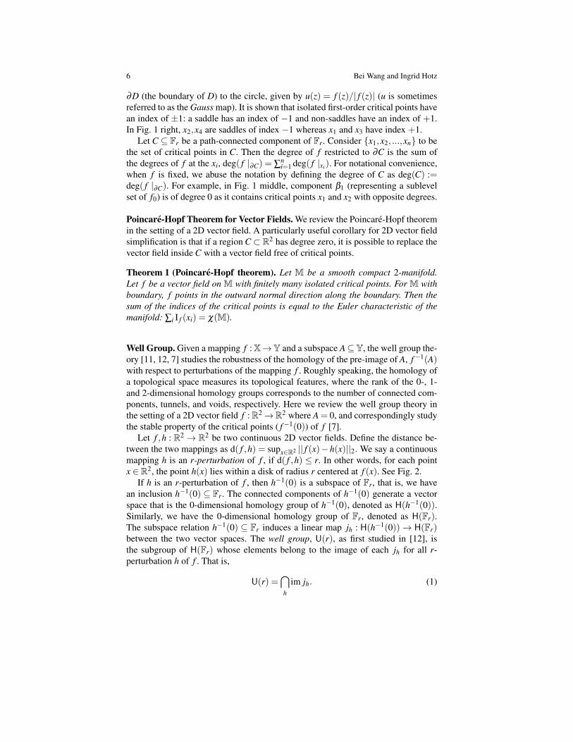
∂D (the boundary of D) to the circle, given by u(z) = f (z)/| f (z)| (u is sometimesreferred to as the Gauss map). It is shown that isolated first-order critical points havean index of ±1: a saddle has an index of −1 and non-saddles have an index of +1.In Fig. 1 right, x2,x4 are saddles of index −1 whereas x1 and x3 have index +1.
Let C ⊆ Fr be a path-connected component of Fr. Consider x1,x2, ...,xn to bethe set of critical points in C. Then the degree of f restricted to ∂C is the sum ofthe degrees of f at the xi, deg( f |∂C) = ∑
ni=1 deg( f |xi). For notational convenience,
when f is fixed, we abuse the notation by defining the degree of C as deg(C) :=deg( f |∂C). For example, in Fig. 1 middle, component β1 (representing a sublevelset of f0) is of degree 0 as it contains critical points x1 and x2 with opposite degrees.
Poincare-Hopf Theorem for Vector Fields. We review the Poincare-Hopf theoremin the setting of a 2D vector field. A particularly useful corollary for 2D vector fieldsimplification is that if a region C ⊂ R2 has degree zero, it is possible to replace thevector field inside C with a vector field free of critical points.
Theorem 1 (Poincare-Hopf theorem). Let M be a smooth compact 2-manifold.Let f be a vector field on M with finitely many isolated critical points. For M withboundary, f points in the outward normal direction along the boundary. Then thesum of the indices of the critical points is equal to the Euler characteristic of themanifold: ∑i I f (xi) = χ(M).
Well Group. Given a mapping f : X→Y and a subspace A⊆Y, the well group the-ory [11, 12, 7] studies the robustness of the homology of the pre-image of A, f−1(A)with respect to perturbations of the mapping f . Roughly speaking, the homology ofa topological space measures its topological features, where the rank of the 0-, 1-and 2-dimensional homology groups corresponds to the number of connected com-ponents, tunnels, and voids, respectively. Here we review the well group theory inthe setting of a 2D vector field f : R2→R2 where A = 0, and correspondingly studythe stable property of the critical points ( f−1(0)) of f [7].
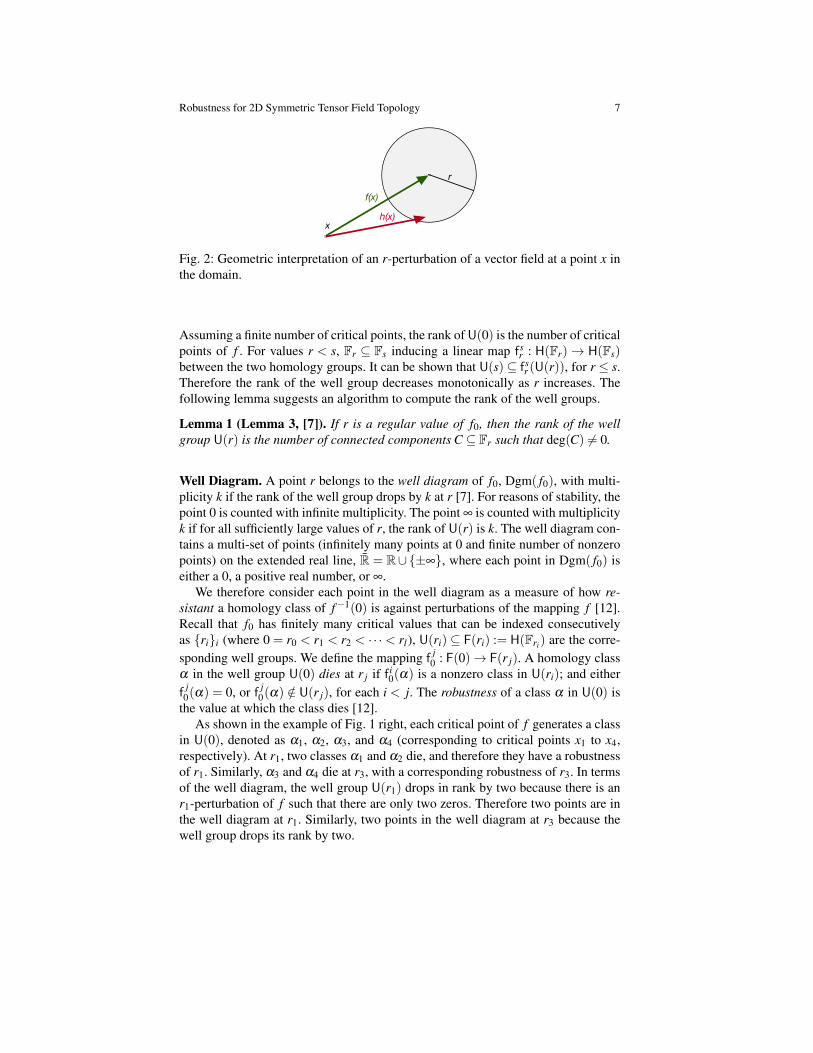
Let f ,h : R2 → R2 be two continuous 2D vector fields. Define the distance be-tween the two mappings as d( f ,h) = supx∈R2 || f (x)−h(x)||2. We say a continuousmapping h is an r-perturbation of f , if d( f ,h) ≤ r. In other words, for each pointx ∈ R2, the point h(x) lies within a disk of radius r centered at f (x). See Fig. 2.
If h is an r-perturbation of f , then h−1(0) is a subspace of Fr, that is, we havean inclusion h−1(0) ⊆ Fr. The connected components of h−1(0) generate a vectorspace that is the 0-dimensional homology group of h−1(0), denoted as H(h−1(0)).Similarly, we have the 0-dimensional homology group of Fr, denoted as H(Fr).The subspace relation h−1(0) ⊆ Fr induces a linear map jh : H(h−1(0))→ H(Fr)between the two vector spaces. The well group, U(r), as first studied in [12], isthe subgroup of H(Fr) whose elements belong to the image of each jh for all r-perturbation h of f . That is,
U(r) =⋂h
im jh. (1)
Robustness for 2D Symmetric Tensor Field Topology 7
r
f(x)
h(x)x
Fig. 2: Geometric interpretation of an r-perturbation of a vector field at a point x inthe domain.
Assuming a finite number of critical points, the rank of U(0) is the number of criticalpoints of f . For values r < s, Fr ⊆ Fs inducing a linear map fs
r : H(Fr)→ H(Fs)between the two homology groups. It can be shown that U(s)⊆ fs
r (U(r)), for r ≤ s.Therefore the rank of the well group decreases monotonically as r increases. Thefollowing lemma suggests an algorithm to compute the rank of the well groups.
Lemma 1 (Lemma 3, [7]). If r is a regular value of f0, then the rank of the wellgroup U(r) is the number of connected components C ⊆ Fr such that deg(C) 6= 0.
Well Diagram. A point r belongs to the well diagram of f0, Dgm( f0), with multi-plicity k if the rank of the well group drops by k at r [7]. For reasons of stability, thepoint 0 is counted with infinite multiplicity. The point ∞ is counted with multiplicityk if for all sufficiently large values of r, the rank of U(r) is k. The well diagram con-tains a multi-set of points (infinitely many points at 0 and finite number of nonzeropoints) on the extended real line, R = R∪±∞, where each point in Dgm( f0) iseither a 0, a positive real number, or ∞.
We therefore consider each point in the well diagram as a measure of how re-sistant a homology class of f−1(0) is against perturbations of the mapping f [12].Recall that f0 has finitely many critical values that can be indexed consecutivelyas rii (where 0 = r0 < r1 < r2 < · · · < rl), U(ri) ⊆ F(ri) := H(Fri) are the corre-sponding well groups. We define the mapping f j
0 : F(0)→ F(r j). A homology classα in the well group U(0) dies at r j if f i
0(α) is a nonzero class in U(ri); and eitherf j0(α) = 0, or f j
0(α) /∈ U(r j), for each i < j. The robustness of a class α in U(0) isthe value at which the class dies [12].
As shown in the example of Fig. 1 right, each critical point of f generates a classin U(0), denoted as α1, α2, α3, and α4 (corresponding to critical points x1 to x4,respectively). At r1, two classes α1 and α2 die, and therefore they have a robustnessof r1. Similarly, α3 and α4 die at r3, with a corresponding robustness of r3. In termsof the well diagram, the well group U(r1) drops in rank by two because there is anr1-perturbation of f such that there are only two zeros. Therefore two points are inthe well diagram at r1. Similarly, two points in the well diagram at r3 because thewell group drops its rank by two.
8 Bei Wang and Ingrid Hotz
Robustness of Critical Points. In the setting of 2D vector fields, the robustnessof a critical point xi can be described by the robustness of the class αi in U(0)that it generates 1. Therefore in our example (Fig. 1), points x1,x2,x3, and x4 haverobustness r1,r1,r3 and r3 respectively.
To compute the robustness of critical points in f , we construct an augmentedmerge tree of f0 that tracks the (connected) components of Fr together with theirdegree information as they appear and merge by increasing r from 0. A leaf noderepresents the creation of a component at a local minima of f0 and an internal noderepresents the merging of components. See [28, 6] for algorithmic details. The ro-bustness of a critical point is the height of its lowest degree zero ancestor in themerge tree. To illustrate the construction, we show a 2D example recreated from [28]in Fig. 1. By definition, the critical points x1 and x2 have robustness r1, whereas x3and x4 have robustness r3. Such a topological notion quantifies the stability of a crit-ical point with respect to perturbations of the vector fields. Intuitively, if a criticalpoint x has robustness r, then it can be canceled with a (r+δ )-perturbation, but notwith any (r−δ )-perturbation, for δ > 0 arbitrarily small.
Given the above machineries, the properties associated with robustness for criti-cal points are direct consequences of Lemma 2 and Lemma 3. Their original proofsketches can be found in the supplementary material of [28]. These proofs, whichare similar to the proof of Lemma 1, are revisited in Section 5.3 for completeness(in the setting of a specific type of vector field).
Lemma 2 (Nonzero Degree Component for Vector Field Perturbation, Corol-lary 1.2 in [28] supplement). Let r be a regular value of f0 and C a connectedcomponent of Fr such that deg(C) 6= 0. Then for any δ -perturbation h of f , whereδ < r, the sum of the degrees of the critical points in h−1(0)∩C is deg(C).
Lemma 3 (Zero Degree Component for Vector Field Perturbation, Corollary1.1 in [28] supplement). Let r be a regular value of f0 and C a connected componentof Fr such that deg(C) = 0. Then, there exists an r-perturbation h of f such that hhas no critical points in C, h−1(0)∩C = /0. In addition, h equals f except possiblywithin the interior of C.
In the example of Fig. 1 right, x1 has a robustness of r1, Lemma 3 implies thatthere exists an (r1 +δ )-perturbation (for an arbitrarily small δ > 0) that can cancelx1 by locally modifying the connected component C ⊆ Fr1+δ containing it.
4 Tensor Fields and Bidirectional Anisotropy Vector Fields
For the remainder of this paper, we consider 2D symmetric second-order tensorfields. In this section, we establish the necessary foundations for introducing a ro-bustness measure for the degenerate points of tensor fields. We introduce the notion
1 We rely on this definition to describe the robustness of a critical point xi, even though the criticalpoint is only a particularly chosen generator of the class αi in U(0).
Robustness for 2D Symmetric Tensor Field Topology 9
of bidirectional anisotropy vectors, which serves two purposes. First, we use it todefine the notion of perturbations of tensor fields for our setting (Section 4.2). Sec-ond, this notion will be central for the definition of the tensor index under the settingof degree theory (Section 5.1).
We start by summarizing some basic concepts of tensor field topology in Sec-tion 4.1. For a complete introduction, we refer the reader to the work by Delmar-celle [9] or Trichoche [25]. Then we introduce the notion of bidirectional anisotropyvector fields in Section 4.2 and discuss its relation with respect to the space of devi-ators. Finally, we establish an isometry from the space of deviators to the anisotropyvector field in Section 4.3.
4.1 Background in Tensor Field Topology
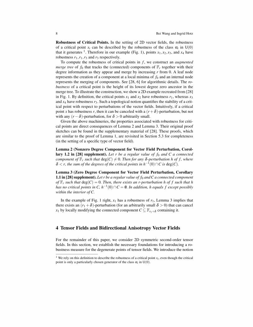
The topology of a 2D symmetric second-order tensor field is defined as the topologyof one of the two eigenvector fields [9]. The degenerate points constitute the basicingredient of the tensor field topology and play a role similar to that for the criticalpoints (zeros) for vector fields.
2D Symmetric Second-Order Tensor Fields. In our setting, a tensor T is a lin-ear operator that associates any vector v to another vector u = T v, where v and uare vectors in the Euclidean vector space R2. In this work, we restrict ourselvesto symmetric tensors. A tensor field T assigns to each position x = (x1,x2) ∈ R2 asymmetric tensor T(x) = T . Let T denote the space of 2D symmetric second-ordertensors over R2. In matrix form, with respect to a given basis of R2, a tensor field Tis defined as
T : R2→T ,T(x) = T =
[t11 t12t12 t22
]. (2)
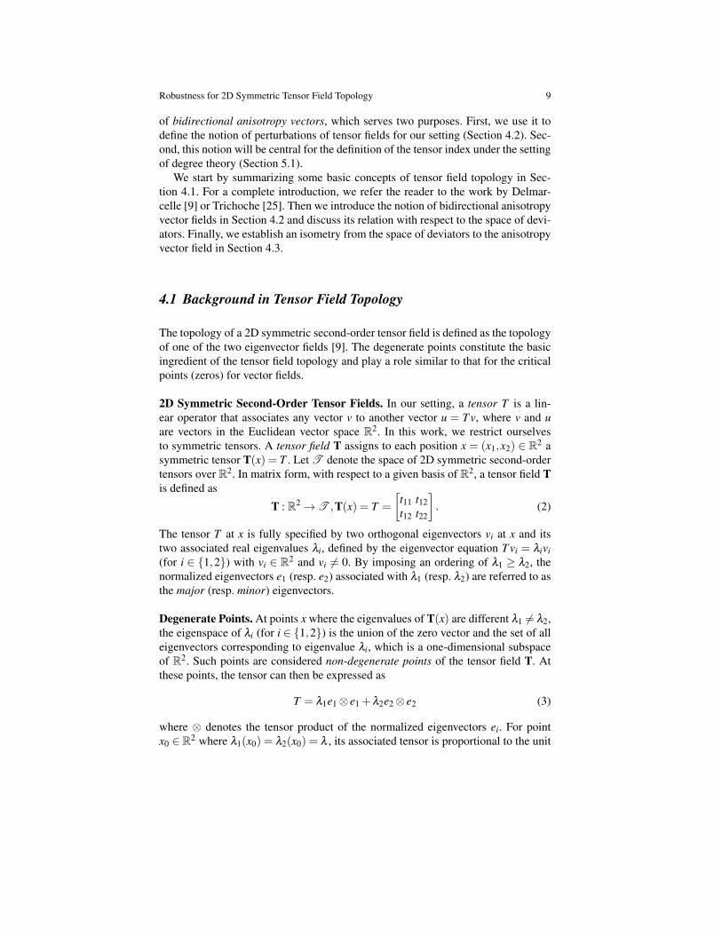
The tensor T at x is fully specified by two orthogonal eigenvectors vi at x and itstwo associated real eigenvalues λi, defined by the eigenvector equation T vi = λivi(for i ∈ 1,2) with vi ∈ R2 and vi 6= 0. By imposing an ordering of λ1 ≥ λ2, thenormalized eigenvectors e1 (resp. e2) associated with λ1 (resp. λ2) are referred to asthe major (resp. minor) eigenvectors.
Degenerate Points. At points x where the eigenvalues of T(x) are different λ1 6= λ2,the eigenspace of λi (for i ∈ 1,2) is the union of the zero vector and the set of alleigenvectors corresponding to eigenvalue λi, which is a one-dimensional subspaceof R2. Such points are considered non-degenerate points of the tensor field T. Atthese points, the tensor can then be expressed as
T = λ1e1⊗ e1 +λ2e2⊗ e2 (3)
where ⊗ denotes the tensor product of the normalized eigenvectors ei. For pointx0 ∈ R2 where λ1(x0) = λ2(x0) = λ , its associated tensor is proportional to the unit
10 Bei Wang and Ingrid Hotz
tensor and the corresponding eigenspace is the entire vector space R2. Its matrixrepresentation is independent from the frame of reference, given as
T (x0) =
[λ 00 λ
].
The points x0 are called degenerate points. In the following sections, we assume thatthese points are isolated points in R2, which is usually the case. While the degeneratepoints as isotropic points exhibiting a high symmetry, they are structurally the mostimportant features for the eigenvector fields.
Real Projective Line. Before we proceed, we need the notion of real projective lineand the homeomorphism between the real projective line and the circle. The realprojective line, denoted as RP1 (or P1 for short), can be thought of as the set of linesthrough the origin of R2, formally P1 := (R2 \0)/∼, for the equivalence relationx ∼ y iff x = cy for some nonzero c ∈ R. We sketch the proof below for P1 beinghomeomorphic to a circle S1, via P1 ' (S1/∼)' S1.
The quotient topology of a real projective line can be described by the mappingη : R2 \ 0 → P1 that sends a point x ∈ R2 \ 0 to its equivalent class [x]. η
is surjective and has the property that η(x) = η(y) iff x ∼ y. Restricting such amapping to S1, we obtain a mapping η |S1 : S1→ P1 that identifies the two antipodalpoints. We now consider S1 as z ∈ C | ||z||= 1. Then we have η |S1(z) = [z]. It iseasy to show that η |S1 defines a homeomorphism between P1 and S1/∼ (where ∼describes the equivalence of z ∼ −z) since η |S1 has the property that U ⊂ (S1/ ∼)is open (w.r.t. quotient topology on S1/∼) iff (η |S1)−1(U) is open in R2 \0.
Now consider the mapping θ : S1→ S1 defined as θ(z) = z2. θ is a continuoussurjective function such that θ(z) = θ(−z). Following the universal property (ofquotient topology2), there exists a unique continuous homeomorphism φ : (S1/ ∼)→ S1 by having θ descending to the quotient. Therefore (S1/∼)' S1.
Eigenvector Fields. In the following section, we describe the construction of aneigenvector field associated with the tensor field T. As described before, a real 2Dsymmetric tensor T at x has two (not necessarily distinct) real eigenvalues λ1 ≥ λ2with associated eigenvectors v1 and v2. It is important to note that neither norm nororientation is defined for the eigenvectors via the eigenvector equation, that is, if vi isan eigenvector, then so is cvi for any nonzero c∈R. The normalized eigenvectors aredenoted as ei (for i ∈ 1,2), where ei ∈ S1. This point of view is reflected throughthe interpretation of an eigenvector as elements of the real projective line. Thuswe define the two eigenvector fields as the mapping ψψψ i : R2→ P1 (for i ∈ 1,2),referred to as the major and minor eigenvector fields, respectively:
2 The quotient space X/∼ together with the quotient map q : X→ (X/∼) is characterized by thefollowing universal property: If g : X→ Z is a continuous map such that a∼ b implies g(a) = g(b)for all a and b in X, then there exists a unique continuous map f : (X/∼)→ Z such that g = f q.We say that g descends to the quotient.
Robustness for 2D Symmetric Tensor Field Topology 11
ψψψ i : R2→ P1,x 7→
[ei] if λ1 6= λ2[e0] for degenerate points, if λ1 = λ2
(4)
[e0] is an arbitrary chosen element of P1. Note that the eigenvector field is not con-tinuous in degenerate points, and in general it is not possible to define [e0] such thatit becomes continuous. From now on, we restrict our attention to the major eigenvec-tor field, referred to as the eigenvector field of T, denoted as ψψψ := ψψψ1, as the minoreigenvectors are always orthogonal and do not provide additional information in the2D case.
The eigenvector fields and the degenerate points constitute the basic ingredientsof the topological structure of a tensor field, and they build the basics for the bi-directional anisotropy vector fields that will be defined in Section 4.2.
4.2 Space of Bidirectional Anisotropy Vectors
In this section, we define the space of bidirectional anisotropy vectors equipped witha distance measure that is based on the L2 norm of vectors. A comparison with thecommonly used distance measure for tensors using the Frobenius norm shows thatthis space is topological equivalent to the space of deviators D . The bidirectionalanisotropy vectors constitute a step toward the definition of an anisotropy vectorfield later used in the study of robustness.
x
y
t11
t22
t12
T
t11 =-t22
D(T)Ω
= ([e1],A)
([e2 ],A)
Ω(T )
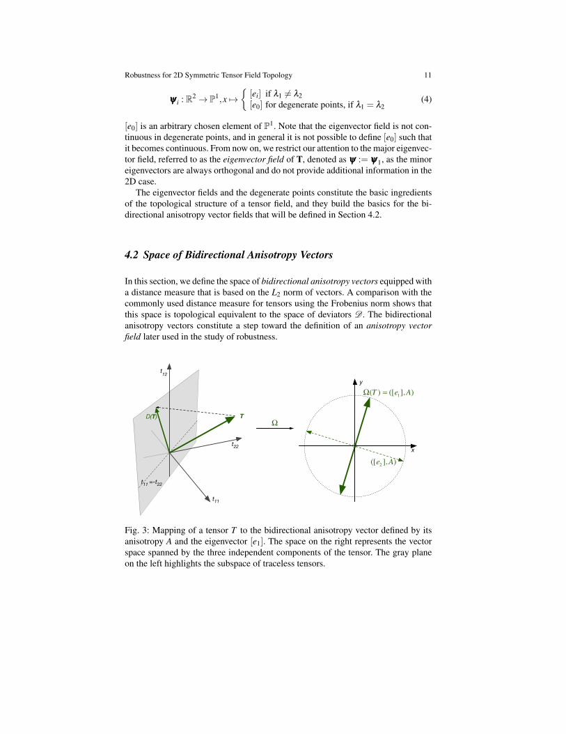
Fig. 3: Mapping of a tensor T to the bidirectional anisotropy vector defined by itsanisotropy A and the eigenvector [e1]. The space on the right represents the vectorspace spanned by the three independent components of the tensor. The gray planeon the left highlights the subspace of traceless tensors.
12 Bei Wang and Ingrid Hotz
Bidirectional Anisotropy Vectors. We define bidirectional anisotropy vectors asbidirectional vectors ω whose direction is defined by the equivalence class of themajor eigenvector [e1] and a norm given by the tensors anisotropy A (e.g., A =|λ1−λ2|). Formally, we consider these vectors as elements of P1×R≥0. Degeneratepoints, that is, points with zero anisotropy and an undefined major eigenvector, arerepresented as the zero vectors.
Let T be the space of 2D symmetric tensors over R2. For each tensor T ∈ T ,we define the bidirectional anisotropy vector by the following mapping (Fig. 3):
Ω : T → P1×R≥0
T 7→ Ω(T ) = ω =
([e1],A) if λ1 6= λ2([e0],0) for degenerate points, if λ1 = λ2
(5)
The space P1×R≥0 can also be interpreted as (R2/∼), for the equivalence relationx∼ y iff x =−y. In this setting, ω is equal to the equivalence class [Ae1] = v,−vconsisting of the two vectors v = Ae1 ∈ R2 and −v = −Ae1 ∈ R2 with e1 ∈ [e1].
α
d(ω ,ω ')
ωω '
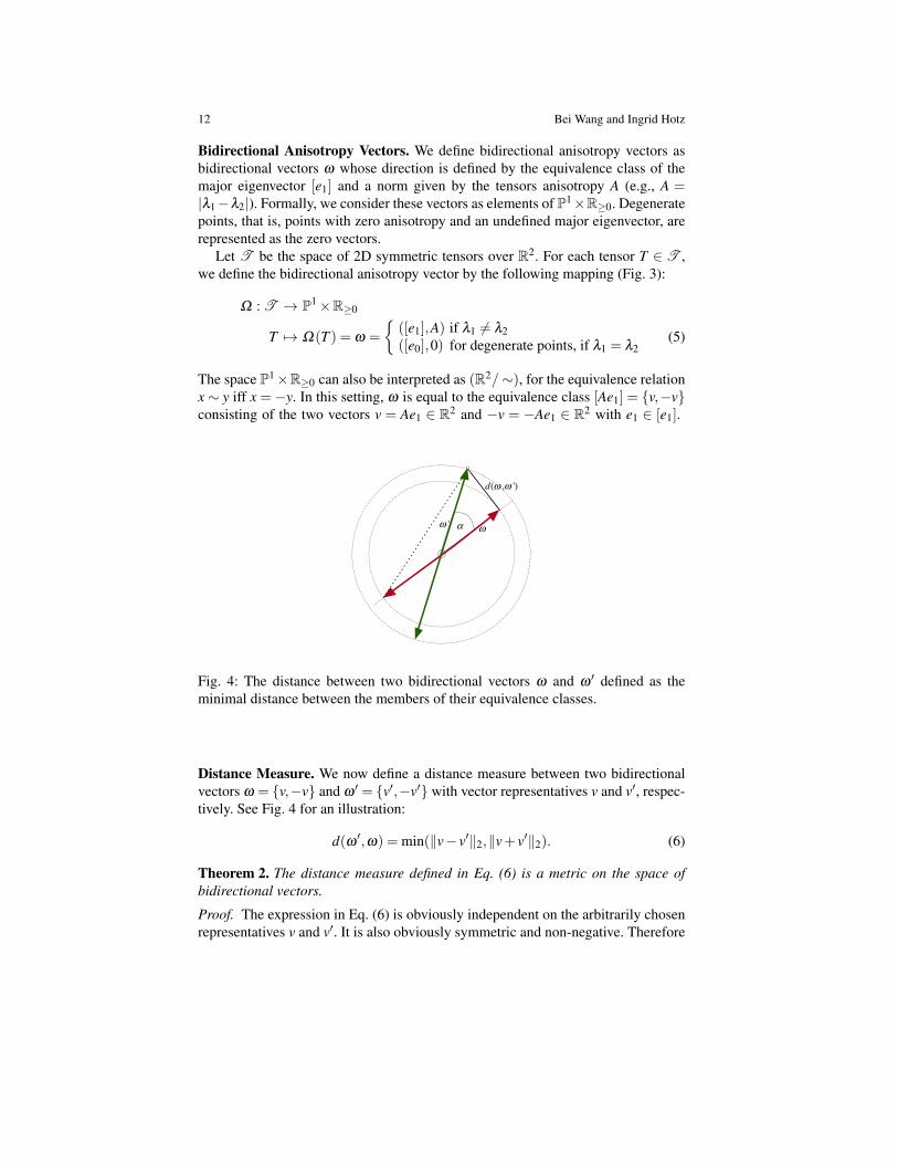
Fig. 4: The distance between two bidirectional vectors ω and ω ′ defined as theminimal distance between the members of their equivalence classes.
Distance Measure. We now define a distance measure between two bidirectionalvectors ω = v,−v and ω ′ = v′,−v′ with vector representatives v and v′, respec-tively. See Fig. 4 for an illustration:
d(ω ′,ω) = min(‖v− v′‖2,‖v+ v′‖2). (6)
Theorem 2. The distance measure defined in Eq. (6) is a metric on the space ofbidirectional vectors.
Proof. The expression in Eq. (6) is obviously independent on the arbitrarily chosenrepresentatives v and v′. It is also obviously symmetric and non-negative. Therefore
Robustness for 2D Symmetric Tensor Field Topology 13
we have: d(ω,ω ′) = 0⇔min(‖v−v′‖2,‖v+v′‖2) = 0⇔ v = v′ or v =−v′ ⇔ω =ω ′. Furthermore the triangle inequality is satisfied (see Appendix B for derivations).Thus Eq. (6) defines a metric on the space of bidirectional vector fields.
Space of Deviators. The space of bidirectional anisotropy vectors is closely relatedto the space of deviatoric tensors D . A deviator D is the traceless or anisotropic partof a tensor T :
D = T − tr(T )2
I, (7)
where I represents the unit tensor. The space of 2D symmetric deviatoric tensors Dis a subspace of the set of 2D symmetric tensors T (see Fig. 3). The eigenvectors ofD coincide with the eigenvectors of T . Thus the deviator field has the same topologyas the original tensor field. Its eigenvalues are δ1 = −δ2 = 1
2 (λ1− λ2). The mostcommonly used norm in T is the Frobenius norm. For the deviator, the Frobeniusnorm is ‖D‖F = 1
2 |λ1 − λ2|, which corresponds to an anisotropy measure (shearstress) that is typically used for failure analysis in mechanical engineering and willbe used as the anisotropy measure A below, that is, let A = |λ1−λ2|. Based on theFrobenius norm, degenerate points are the points x0 at which ‖D(x0)‖F = 0. TheFrobenius norm therefore induces a metric on D , that is, for D,D′ ∈D :
dF(D,D′) = ‖D−D′‖F . (8)
Deviator and Bidirectional Vectors. If we restrict the mapping Ω | defined inEq. (5) to the space of deviatoric tensors D , the resulting mapping Ω |D is one-to-one. The inverse mapping is then defined by
(Ω |D )−1 : P1×R≥0 → D
ω = [Ae] 7→ D =
√A
2e⊗ e−
√A
2e⊥⊗ e⊥. (9)
Here e⊥ represents a normalized vector orthogonal to e. It can be seen immediatelythat this expression is independent on the sign of the representative vector e and thusis well-defined. For ω = [0e0], Eq. 9 results in a zero tensor that is independent onthe chosen vector e0.
Theorem 3. For the above defined metric Eq. (6) on the space of bidirectionalanisotropy vectors and the Frobenius metric Eq. (8) on the space of deviators, wehave
Ω(D′) ∈ Br(Ω(D))⇒ D′ ∈ Br′(D) (10)
with r′ =√
5r. For the opposite direction, we have
D′ ∈ Br′(D)⇒Ω(D′) ∈ Br(Ω(D)). (11)
Thus the mapping defined in Eq. (5) is continuous, and the space of tensor deviatorsand the bidirectional anisotropy vectors are topologically equivalent.
14 Bei Wang and Ingrid Hotz
Proof. Let D and D′ be two symmetric, traceless 2D tensors with major eigen-values ( 1√
2λ , −1√
2λ ) and ( 1√
2µ, −1√
2µ), respectively, as well as their corresponding
eigenvectors [ei] and [ fi], for i = 1,2. Their norms are given by ‖D‖2F = λ 2 and
‖D′‖2F = µ2. The corresponding bidirectional anisotropy vectors are defined as
ω = Ω(D) = [Ae1] with A = λ and ω ′ = Ω(D′) = [A′ f1] with A′ = µ .In order to compare the Frobenius distance between deviators and the distance
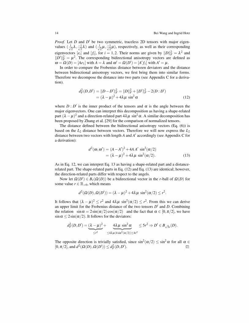
between bidirectional anisotropy vectors, we first bring them into similar forms.Therefore we decompose the distance into two parts (see Appendix C for a deriva-tion).
d2F(D,D′) = ‖D−D′‖2
F = ‖D‖2F +‖D′‖2
F −2(D : D′)
= (λ −µ)2 +4λ µ sin2α (12)
where D : D′ is the inner product of the tensors and α is the angle between themajor eigenvectors. One can interpret this decomposition as having a shape-relatedpart (λ −µ)2 and a direction-related part 4λ µ sin2
α . A similar decomposition hasbeen proposed by Zhang et al. [29] for the comparison of normalized tensors.
The distance defined between the bidirectional anisotropy vectors (Eq. (6)) isbased on the L2 distance between vectors. Therefore we will now express the L2distance between two vectors with length A and A′ accordingly (see Appendix C fora derivation):
d2(ω,ω ′) = (A−A′)2 +4A A′ sin2(α/2)= (λ −µ)2 +4λ µ sin2(α/2). (13)
As in Eq. 12, we can interpret Eq. 13 as having a shape-related part and a distance-related part. The shape-related parts in Eq. (12) and Eq. (13) are identical; however,the direction-related parts differ with respect to the angels.
Now let Ω(D′) ∈ Br(Ω(D)) be a bidirectional vector in the r-ball of Ω(D) forsome value r ∈ R>0, which means
d2(Ω(D),Ω(D′)) = (λ −µ)2 +4λ µ sin2(α/2)≤ r2.
It follows that (λ − µ)2 ≤ r2 and 4λ µ sin2(α/2) ≤ r2. From this we can derivean upper limit for the Frobenius distance of the two tensors D′ and D. Combiningthe relation sinα = 2sin(α/2)cos(α/2) and the fact that α ∈ [0,π/2], we havesinα ≤ 2sin(α/2). It follows for the deviators:
d2F(D,D′) = (λ −µ)2︸ ︷︷ ︸
≤r2
+ 4λ µ sin2α︸ ︷︷ ︸
≤4λ µ(4sin2(α/2))≤4r2
≤ 5r2⇒ D′ ∈ B√5r(D).
The opposite direction is trivially satisfied, since sin2(α/2) ≤ sin2α for all α ∈
[0,π/2], and d2(Ω(D),Ω(D′))≤ d2F(D,D′).
Robustness for 2D Symmetric Tensor Field Topology 15
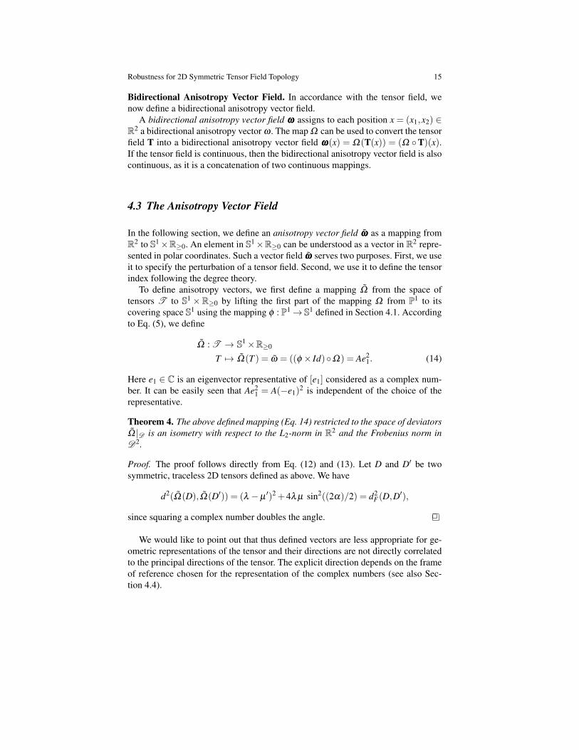
Bidirectional Anisotropy Vector Field. In accordance with the tensor field, wenow define a bidirectional anisotropy vector field.
A bidirectional anisotropy vector field ωωω assigns to each position x = (x1,x2) ∈R2 a bidirectional anisotropy vector ω . The map Ω can be used to convert the tensorfield T into a bidirectional anisotropy vector field ωωω(x) = Ω(T(x)) = (Ω T)(x).If the tensor field is continuous, then the bidirectional anisotropy vector field is alsocontinuous, as it is a concatenation of two continuous mappings.
4.3 The Anisotropy Vector Field
In the following section, we define an anisotropy vector field ωωω as a mapping fromR2 to S1×R≥0. An element in S1×R≥0 can be understood as a vector in R2 repre-sented in polar coordinates. Such a vector field ωωω serves two purposes. First, we useit to specify the perturbation of a tensor field. Second, we use it to define the tensorindex following the degree theory.
To define anisotropy vectors, we first define a mapping Ω from the space oftensors T to S1×R≥0 by lifting the first part of the mapping Ω from P1 to itscovering space S1 using the mapping φ : P1→ S1 defined in Section 4.1. Accordingto Eq. (5), we define
Ω : T → S1×R≥0
T 7→ Ω(T ) = ω = ((φ × Id)Ω) = Ae21. (14)
Here e1 ∈ C is an eigenvector representative of [e1] considered as a complex num-ber. It can be easily seen that Ae2
1 = A(−e1)2 is independent of the choice of the
representative.
Theorem 4. The above defined mapping (Eq. 14) restricted to the space of deviatorsΩ |D is an isometry with respect to the L2-norm in R2 and the Frobenius norm inD2.
Proof. The proof follows directly from Eq. (12) and (13). Let D and D′ be twosymmetric, traceless 2D tensors defined as above. We have
d2(Ω(D),Ω(D′)) = (λ −µ′)2 +4λ µ sin2((2α)/2) = d2
F(D,D′),
since squaring a complex number doubles the angle.
We would like to point out that thus defined vectors are less appropriate for ge-ometric representations of the tensor and their directions are not directly correlatedto the principal directions of the tensor. The explicit direction depends on the frameof reference chosen for the representation of the complex numbers (see also Sec-tion 4.4).
16 Bei Wang and Ingrid Hotz
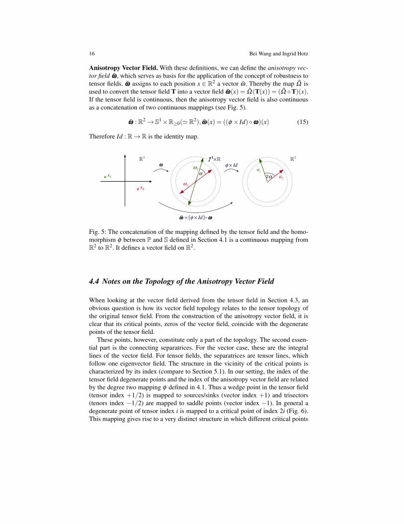
Anisotropy Vector Field. With these definitions, we can define the anisotropy vec-tor field ωωω , which serves as basis for the application of the concept of robustness totensor fields. ωωω assigns to each position x ∈ R2 a vector ω . Thereby the map Ω isused to convert the tensor field T into a vector field ωωω(x) = Ω(T(x)) = (Ω T)(x).If the tensor field is continuous, then the anisotropy vector field is also continuousas a concatenation of two continuous mappings (see Fig. 5).
ωωω : R2→ S1×R≥0(' R2), ωωω(x) = ((φ × Id)ωωω)(x) (15)
Therefore Id : R→ R is the identity map.
!2
α
x2
x1 α2
ω×!
a1ω1
a2ω 2
!2
φ × Id
!ω = φ × Id( )"ω
Fig. 5: The concatenation of the mapping defined by the tensor field and the homo-morphism φ between P and S defined in Section 4.1 is a continuous mapping fromR2 to R2. It defines a vector field on R2.
4.4 Notes on the Topology of the Anisotropy Vector Field
When looking at the vector field derived from the tensor field in Section 4.3, anobvious question is how its vector field topology relates to the tensor topology ofthe original tensor field. From the construction of the anisotropy vector field, it isclear that its critical points, zeros of the vector field, coincide with the degeneratepoints of the tensor field.
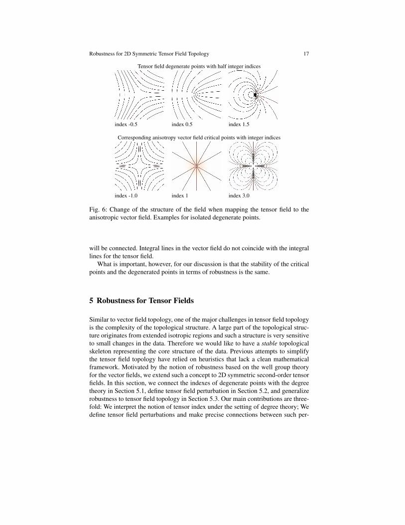
These points, however, constitute only a part of the topology. The second essen-tial part is the connecting separatrices. For the vector case, these are the integrallines of the vector field. For tensor fields, the separatrices are tensor lines, whichfollow one eigenvector field. The structure in the vicinity of the critical points ischaracterized by its index (compare to Section 5.1). In our setting, the index of thetensor field degenerate points and the index of the anisotropy vector field are relatedby the degree two mapping φ defined in 4.1. Thus a wedge point in the tensor field(tensor index +1/2) is mapped to sources/sinks (vector index +1) and trisectors(tenors index −1/2) are mapped to saddle points (vector index −1). In general adegenerate point of tensor index i is mapped to a critical point of index 2i (Fig. 6).This mapping gives rise to a very distinct structure in which different critical points
Robustness for 2D Symmetric Tensor Field Topology 17
Tensor field degenerate points with half integer indices
index -0.5 index 0.5 index 1.5
Corresponding anisotropy vector field critical points with integer indices
index -1.0 index 1 index 3.0
Fig. 6: Change of the structure of the field when mapping the tensor field to theanisotropic vector field. Examples for isolated degenerate points.
will be connected. Integral lines in the vector field do not coincide with the integrallines for the tensor field.
What is important, however, for our discussion is that the stability of the criticalpoints and the degenerated points in terms of robustness is the same.
5 Robustness for Tensor Fields
Similar to vector field topology, one of the major challenges in tensor field topologyis the complexity of the topological structure. A large part of the topological struc-ture originates from extended isotropic regions and such a structure is very sensitiveto small changes in the data. Therefore we would like to have a stable topologicalskeleton representing the core structure of the data. Previous attempts to simplifythe tensor field topology have relied on heuristics that lack a clean mathematicalframework. Motivated by the notion of robustness based on the well group theoryfor the vector fields, we extend such a concept to 2D symmetric second-order tensorfields. In this section, we connect the indexes of degenerate points with the degreetheory in Section 5.1, define tensor field perturbation in Section 5.2, and generalizerobustness to tensor field topology in Section 5.3. Our main contributions are three-fold: We interpret the notion of tensor index under the setting of degree theory; Wedefine tensor field perturbations and make precise connections between such per-
18 Bei Wang and Ingrid Hotz
turbations with the perturbations of bidirectional anisotropy vector fields; And wegeneralize the notion of robustness to tensor field topology.
5.1 Indexes of Degenerate Points and Degree Theory
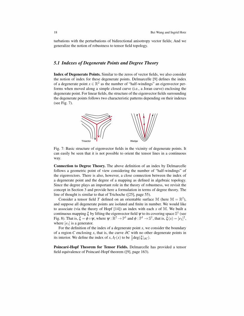
Index of Degenerate Points. Similar to the zeros of vector fields, we also considerthe notion of index for these degenerate points. Delmarcelle [9] defines the indexof a degenerate point x ∈ R2 as the number of “half-windings” an eigenvector per-forms when moved along a simple closed curve (i.e., a Joran curve) enclosing thedegenerate point. For linear fields, the structure of the eigenvector fields surroundingthe degenerate points follows two characteristic patterns depending on their indexes(see Fig. 7).
Trisector Wedge
Fig. 7: Basic structure of eigenvector fields in the vicinity of degenerate points. Itcan easily be seen that it is not possible to orient the tensor lines in a continuousway.
Connection to Degree Theory. The above definition of an index by Delmarcellefollows a geometric point of view considering the number of “half-windings” ofthe eigenvectors. There is also, however, a close connection between the index ofa degenerate point and the degree of a mapping as defined in algebraic topology.Since the degree plays an important role in the theory of robustness, we revisit theconcept in Section 3 and provide here a formulation in terms of degree theory. Theline of thought is similar to that of Trichoche ([25], page 55).
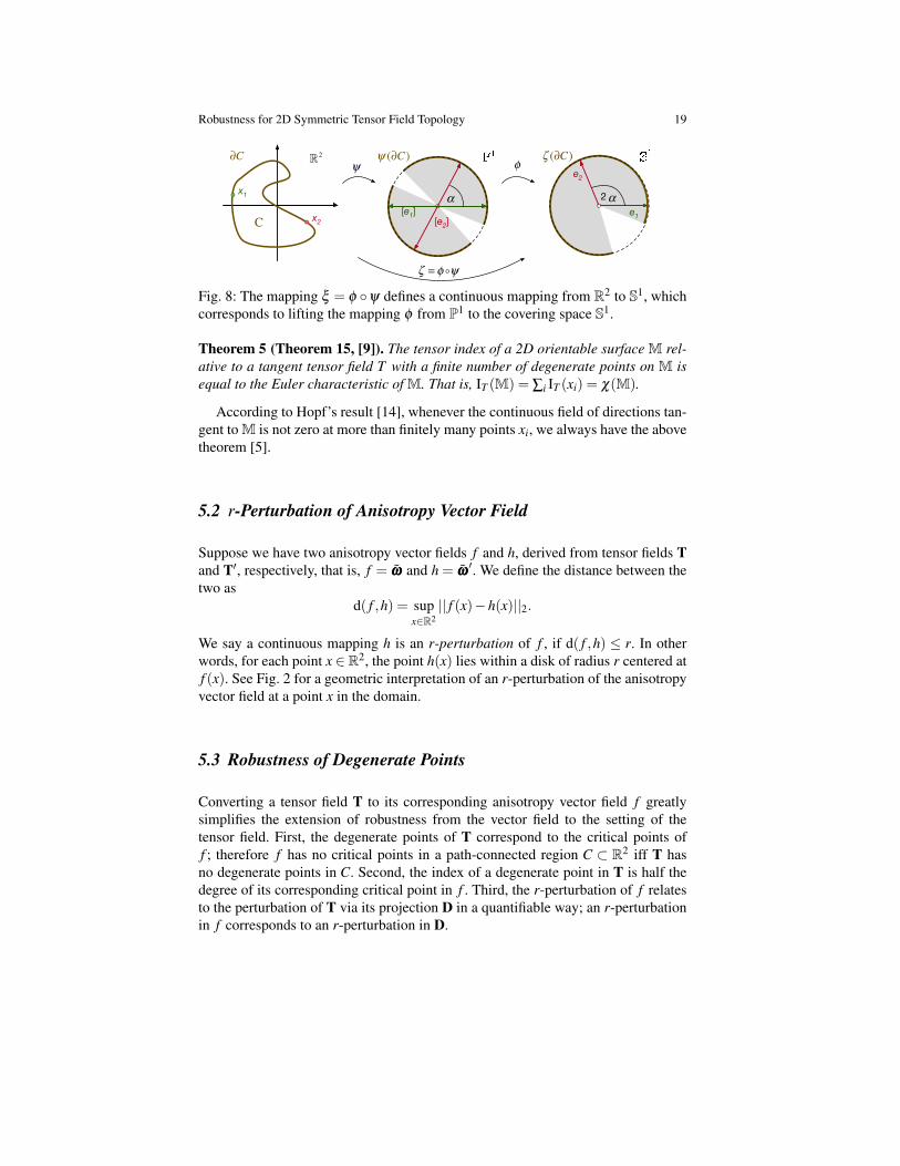
Consider a tensor field T defined on an orientable surface M (here M = R2),and suppose all degenerate points are isolated and finite in number. We would liketo associate (via the theory of Hopf [14]) an index with each x of M. We built acontinuous mapping ξ by lifting the eigenvector field ψ to its covering space S1 (seeFig. 8). That is, ξ = φ ψ , where ψ : R2→ P1 and φ : P1→ S1, that is, ξ (x) = [e1]
2,where [e1] is a generator.
For the definition of the index of a degenerate point x, we consider the boundaryof a region C enclosing x, that is, the curve ∂C with no other degenerate points inits interior. We define the index of x, IT (x) to be 1
2 deg(ξ |∂C).
Poincare-Hopf Theorem for Tensor Fields. Delmarcelle has provided a tensorfield equivalence of Poincare-Hopf theorem ([9], page 163).
Robustness for 2D Symmetric Tensor Field Topology 19
±v1 ±v2
!2
αx2
x1 αe1
e2
2
C
∂Cφψ
[e2][e1]
ψ (∂C)
ζ = φ !ψ
ζ (∂C)
Fig. 8: The mapping ξ = φ ψ defines a continuous mapping from R2 to S1, whichcorresponds to lifting the mapping φ from P1 to the covering space S1.
Theorem 5 (Theorem 15, [9]). The tensor index of a 2D orientable surface M rel-ative to a tangent tensor field T with a finite number of degenerate points on M isequal to the Euler characteristic of M. That is, IT (M) = ∑i IT (xi) = χ(M).
According to Hopf’s result [14], whenever the continuous field of directions tan-gent to M is not zero at more than finitely many points xi, we always have the abovetheorem [5].
5.2 r-Perturbation of Anisotropy Vector Field
Suppose we have two anisotropy vector fields f and h, derived from tensor fields Tand T′, respectively, that is, f = ωωω and h = ωωω
′. We define the distance between thetwo as
d( f ,h) = supx∈R2|| f (x)−h(x)||2.
We say a continuous mapping h is an r-perturbation of f , if d( f ,h) ≤ r. In otherwords, for each point x ∈R2, the point h(x) lies within a disk of radius r centered atf (x). See Fig. 2 for a geometric interpretation of an r-perturbation of the anisotropyvector field at a point x in the domain.
5.3 Robustness of Degenerate Points
Converting a tensor field T to its corresponding anisotropy vector field f greatlysimplifies the extension of robustness from the vector field to the setting of thetensor field. First, the degenerate points of T correspond to the critical points off ; therefore f has no critical points in a path-connected region C ⊂ R2 iff T hasno degenerate points in C. Second, the index of a degenerate point in T is half thedegree of its corresponding critical point in f . Third, the r-perturbation of f relatesto the perturbation of T via its projection D in a quantifiable way; an r-perturbationin f corresponds to an r-perturbation in D.
20 Bei Wang and Ingrid Hotz
We have conjectured that the robustness of degenerate points x for tensor fieldsT would resemble the robustness of its corresponding critical point f for theanisotropy vector fields. Recall that, by definition, f is an anisotropy vector field,f : R2→ R2, f0 = || f ||2 : R2→ R , Fr = f−1
0 (−∞,r]. Let h be another anisotropyvector field h : R2→ R2. We would prove the following lemmas, whose proofs areidentical to the proofs used for results in [28] (Corollary 1.1 and Corollary 1.2 inthe supplemental material) with respect to vector field perturbation. We include theproofs here for completeness.
Lemma 4 (Nonzero Degree Component for Tensor Field Perturbation). Let r bea regular value of f0 and C a connected component of Fr such that deg(C) 6= 0. Thenfor any δ -perturbation h of f , where δ < r, the sum of the degrees of the criticalpoints in h−1(0)∩C is deg(C).
Proof. Before we illustrate the details of the proof, we need to provide a rigorousdefinition of the degree of a mapping.
Let C ⊆ Fr be a path-connected component of Fr. Function f restricted to C,denoted f |C : (C,∂C)→ (Br,∂Br), maps C to the closed ball Br of radius r centeredat the origin, where ∂ is the boundary operator. f |C induces a homomorphism on thehomology level, f∗|C : H(C,∂C)→H(Br,∂Br). Let µC and µBr be the generators ofH(C,∂C) and H(Br,∂Br), respectively. The degree of C (more precisely the degreeof f |C), deg(C) = deg( f |C), is the unique integer such that f∗|C(µC) = deg(C) ·µBr .Furthermore we have the function restricted to the boundary, that is, f |∂C : ∂C→ S1.It was shown that deg( f |C) = deg( f |∂C) ([7], Lemma 1).
Consider the following diagram for any δ -perturbation h of f , where δ < r:
H(C,∂C)i∗−→ H(C,C−h−1(0))
↓ f∗|C ↓ h∗|0H(Br,∂Br)
j∗−→ H(Br,Br−0). (16)
i∗ and j∗ are homomorphisms induced by space-level inclusions i : (C,∂C) →(C,C−h−1(0)) and j : (Br,∂Br)→ (Br,Br−0). j∗ is also an isomorphism. Thevertical maps f∗|C and h∗|0 are induced by f and h with restrictions, respectively.Therefore the diagram commutes.
Suppose r is a regular value and deg(C) 6= 0. Then by commutativity, the sum ofdegrees of the critical points in h−1(0)∩C is deg(C).
Lemma 5 (Zero Degree Component for Tensor Field Perturbation). Let r be aregular value of f0 and C a connected component of Fr such that deg(C) = 0. Thenthere exists an r-perturbation h of f such that h has no degenerate points in C,h−1(0)∩C = /0. In addition, h equals f except possibly within the interior of C.
Proof. The proof follows the commutative diagram above (Eq. 16) for any r-perturbation h of f . Suppose r is a regular value. Then well groups U(r − δ )and U(r + δ ) are isomorphic for all sufficiently small δ > 0. Suppose deg(C) =
Robustness for 2D Symmetric Tensor Field Topology 21
deg( f |C) = deg( f |∂C) = 0. Then following the Hopf Extension Theorem ([13], page145), if the function f |∂C : ∂C→ S1 has degree zero, then f can be extended to aglobally defined map g : C→ S1 such that g equals f when both are restricted to∂C. Now we define a perturbation h : R2→R2 such that h = 0.5 · f +0.5 ·g. h is themidpoint on a straight line homotopy between f and g. By definition d(h, f )≤ r, soh is an r-perturbation of f . In addition, h−1(0)∩C is empty.
Remark. One important aspect of well group theory is that the well group is definedto be the intersection of the images of jh for all r-perturbation h of f (Eq. 1). Givenf as an anisotropy vector field, we introduce an r-perturbation h of f . We wouldneed to make sure that any such h is itself a valid anisotropy vector field. That is,for any r-perturbation h of f , there exists a corresponding tensor field T from whichan anisotropy vector field h can be derived. This is true based on derivations inSection 4.
6 Discussion
There are a few challenges in extending our framework to a 3D symmetric tensorfield. The notion of deviator can be generalized to 3D, but the notion of anisotropyvector field does not generalize to 3D. The lack of such a notion poses a challengein studying robustness for 3D symmetric tensor field topology via transformation ofthe data to the anisotropy vector field. We suspect a possible solution is to defineperturbations with respect to the bidirectional anisotropy vector field derived fromeigenvector fields.
An important contribution of this paper is the conversion from a tensor field Tto its corresponding anisotropy vector field f . There is a one-to-one correspondencebetween the degenerate points of T and the critical points of f . However, as shownin Fig. 6, the topology of T and that of f obviously do not agree. Understandingtheir differences and the consequences will be an interesting direction.
The main motivation of extending robustness to 2D symmetric tensor field is thatit would lead to simplification schemes for tensor field data. In general, topology-based simplification techniques pair the topological features for simplification viathe computation of topological skeleton, which can be numerically unstable. In con-trast, the proposed robustness-based method is independent of the topological skele-ton and, thus, is insensitive to numerical error.
22 Bei Wang and Ingrid Hotz
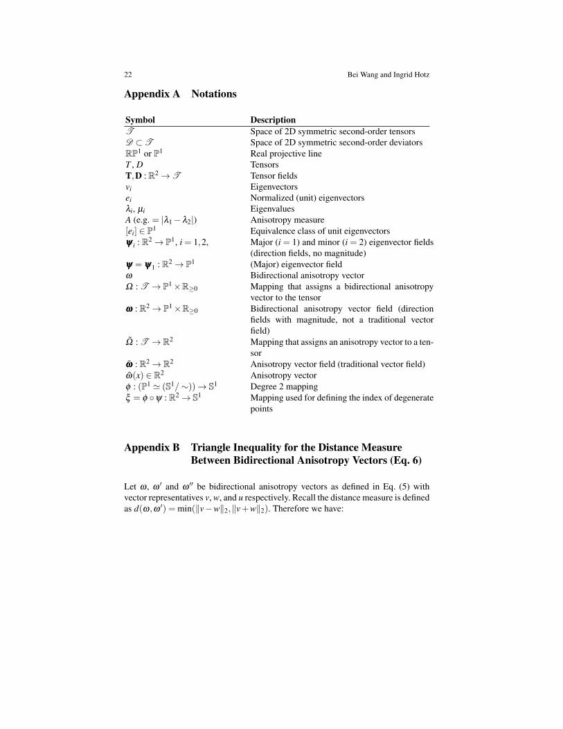
Appendix A Notations
Symbol DescriptionT Space of 2D symmetric second-order tensorsD ⊂T Space of 2D symmetric second-order deviatorsRP1 or P1 Real projective lineT , D TensorsT,D : R2→T Tensor fieldsvi Eigenvectorsei Normalized (unit) eigenvectorsλi, µi EigenvaluesA (e.g. = |λ1−λ2|) Anisotropy measure[ei] ∈ P1 Equivalence class of unit eigenvectorsψψψ i : R2→ P1, i = 1,2, Major (i = 1) and minor (i = 2) eigenvector fields
(direction fields, no magnitude)ψψψ = ψψψ1 : R2→ P1 (Major) eigenvector fieldω Bidirectional anisotropy vectorΩ : T → P1×R≥0 Mapping that assigns a bidirectional anisotropy
vector to the tensorωωω : R2→ P1×R≥0 Bidirectional anisotropy vector field (direction
fields with magnitude, not a traditional vectorfield)
Ω : T → R2 Mapping that assigns an anisotropy vector to a ten-sor
ωωω : R2→ R2 Anisotropy vector field (traditional vector field)ω(x) ∈ R2 Anisotropy vectorφ : (P1 ' (S1/∼))→ S1 Degree 2 mappingξ = φ ψ : R2→ S1 Mapping used for defining the index of degenerate
points
Appendix B Triangle Inequality for the Distance MeasureBetween Bidirectional Anisotropy Vectors (Eq. 6)
Let ω , ω ′ and ω ′′ be bidirectional anisotropy vectors as defined in Eq. (5) withvector representatives v, w, and u respectively. Recall the distance measure is definedas d(ω,ω ′) = min(‖v−w‖2,‖v+w‖2). Therefore we have:
Robustness for 2D Symmetric Tensor Field Topology 23
d(ω,ω ′)+d(ω ′,ω ′′)= min( ‖v−w‖2,‖v+w‖2)+min(‖w−u‖2,‖w+u‖2)
≥ min( ‖v−w‖2 +‖w−u‖2,‖v−w‖2 +‖w+u‖2,
‖v+w‖2 +‖w−u‖2,‖v+w‖2 +‖w+u‖2 )
= min( ‖v−w‖2 +‖w−u‖2,‖v−w‖2 +‖w− (−u)‖2,
‖v− (−w)‖2 +‖(−w)− (−u)‖2,‖v− (−w)‖2−‖(−w)−u‖2 )
≥ min( ‖v−u‖2,‖v− (−u)‖2,‖v− (−u)‖2,‖v−u‖2 )
= min( ‖v−u‖2,‖v+u‖2 )
= d(ω,ω ′′)
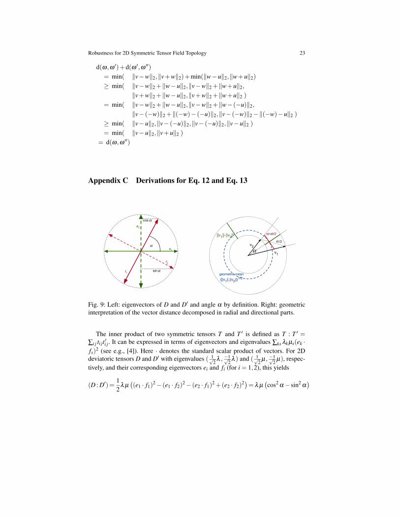
Appendix C Derivations for Eq. 12 and Eq. 13
αe1
e2
f1
f2
cosα
sinα
v1
v2
||v1||-||v2||
geometric mean(||v1||.||v2||)1/2
α
sin /2α
α /2
Fig. 9: Left: eigenvectors of D and D′ and angle α by definition. Right: geometricinterpretation of the vector distance decomposed in radial and directional parts.
The inner product of two symmetric tensors T and T ′ is defined as T : T ′ =∑i j ti jt ′i j. It can be expressed in terms of eigenvectors and eigenvalues ∑ks λkµs(ek ·fs)
2 (see e.g., [4]). Here · denotes the standard scalar product of vectors. For 2Ddeviatoric tensors D and D′ with eigenvalues ( 1√
2λ , −1√
2λ ) and ( 1√
2µ, −1√
2µ), respec-
tively, and their corresponding eigenvectors ei and fi (for i = 1,2), this yields
(D : D′)=12
λ µ((e1 · f1)
2− (e1 · f2)2− (e2 · f1)
2 +(e2 · f2)2)= λ µ
(cos2
α− sin2α)
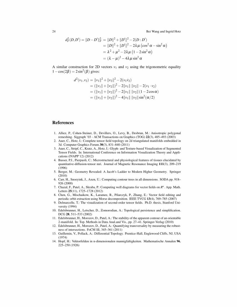
24 Bei Wang and Ingrid Hotz
d2F(D,D′) = ‖D−D′‖2
F = ‖D‖2 +‖D′‖2−2(D : D′)
= ‖D‖2 +‖D′‖2−2λ µ(cos2
α− sin2α)
= λ2 +µ
2−2λ µ(1−2sin2
α)
= (λ −µ)2−4λ µ sin2α
A similar construction for 2D vectors v1 and v2 using the trigonometric equality1− cos(2β ) = 2sin2(β ) gives:
d2(v1,v2) = ‖v1‖2 +‖v2‖2−2(v1v2)
= (‖v1‖+‖v2‖)2−2‖v1‖ ‖v2‖−2(v1 · v2)
= (‖v1‖+‖v2‖)2−2‖v1‖ ‖v2‖(1−2cosα)
= (‖v1‖+‖v2‖)2−4‖v1‖ ‖v2‖sin2(α/2)
References
1. Alliez, P., Cohen-Steiner, D., Devillers, O., Levy, B., Desbrun, M.: Anisotropic polygonalremeshing. Siggraph ’03 - ACM Transactions on Graphics (TOG) 22(3), 485–493 (2003)
2. Auer, C., Hotz, I.: Complete tensor field topology on 2d triangulated manifolds embedded in3d. Computer Graphics Forum 30(3), 831–840 (2011)
3. Auer, C., Stripf, C., Kratz, A., Hotz, I.: Glyph- and Texture-based Visualization of SegmentedTensor Fields. In: International Conference on Information Visualization Theory and Appli-cations (IVAPP’12) (2012)
4. Basser, P.J., Pierpaoli, C.: Microstructural and physiological features of tissues elucidated byquantitative-diffusion-tensor mri. Journal of Magnetic Resonance Imaging 111(3), 209–219(1996)
5. Berger, M.: Geometry Revealed: A Jacob’s Ladder to Modern Higher Geometry. Springer(2010)
6. Carr, H., Snoeyink, J., Axen, U.: Computing contour trees in all dimensions. SODA pp. 918–926 (2000)
7. Chazal, F., Patel, A., Skraba, P.: Computing well diagrams for vector fields on Rn. App. Math.Letters 25(11), 1725–1728 (2012)
8. Chen, G., Mischaikow, K., Laramee, R., Pilarczyk, P., Zhang, E.: Vector field editing andperiodic orbit extraction using Morse decomposition. IEEE TVCG 13(4), 769–785 (2007)
9. Delmarcelle, T.: The visualization of second-order tensor fields. Ph.D. thesis, Stanford Uni-versity (1994)
10. Edelsbrunner, H., Letscher, D., Zomorodian, A.: Topological persistence and simplification.DCG 28, 511–533 (2002)
11. Edelsbrunner, H., Morozov, D., Patel, A.: The stability of the apparent contour of an orientable2-manifold. In: Top. Methods in Data Anal.and Vis., pp. 27–41. Springer-Verlag (2010)
12. Edelsbrunner, H., Morozov, D., Patel, A.: Quantifying transversality by measuring the robust-ness of intersections. FoCM 11, 345–361 (2011)
13. Guillemin, V., Pollack, A.: Differential Topology. Prentice-Hall, Englewood Cliffs, NJ, USA(1974)
14. Hopf, H.: Vektorfelden in n-dimensionalen mannigfaltigkeiten. Mathematische Annalen 96,225–250 (1926)
Robustness for 2D Symmetric Tensor Field Topology 25
15. Hotz, I., Sreevalsan-Nair, J., Hagen, H., Hamann, B.: Tensor field reconstruction based oneigenvector and eigenvalue interpolation. In: H. Hagen (ed.) Scientific Visualization: Ad-vanced Concepts, Dagstuhl Follow-Ups, vol. 1, pp. 110–123. Schloss Dagstuhl–Leibniz-Zentrum fuer Informatik (2010)
16. Kalberer, F., Nieser, M., Polthier, K.: Quadcover - surface parameterization using branchedcoverings. Computer Graphics Forum 26(3), 375–384 (2007)
17. Knoppel, F., Crane, K., Pinkall, U., Schroder, P.: Globally optimal direction fields. ACMTransactions on Graphics 32(4) (2013)
18. Kratz, A., Auer, C., Stommel, M., Hotz, I.: Visualization and Analysis of Second-Order Ten-sors: Moving Beyond the Symmetric Positive-Definite Case. Computer Graphics Forum -State of the Art Reports 32(1), 49–74 (2013)
19. McLoughlin, T., Laramee, R.S., Peikert, R., Post, F.H., Chen, M.: Over two decades ofintegration-based, geometric flow visualization. Computer Graphics Forum 29(6), 1807–1829(2010)
20. Skraba, P., Rosen, P., Wang, B., Chen, G., Bhatia, H., Pascucci, V.: Critical point cancella-tion in 3D vector fields: Robustness and discussion. IEEE Transactions on Visualization andComputer Graphics 22(6), 1683–1693 (2016)
21. Skraba, P., Wang, B.: Interpreting feature tracking through the lens of robustness. Top. Meth-ods in Data Anal. and Vis. III (2014)
22. Skraba, P., Wang, B., Chen, G., Rosen, P.: 2d vector field simplification based on robustness.Proc. Pac. Vis. Symp. (2014)
23. Skraba, P., Wang, B., Chen, G., Rosen, P.: Robustness-based simplification of 2d steady andunsteady vector fields. IEEE TVCG 21(8), 930 – 944 (2015)
24. Sreevalsan-Nair, J., Auer, C., Hamann, B., Hotz, I.: Eigenvector-based interpolation and seg-mentation of 2d tensor fields. In: Topological Methods in Data Analysis and Visualiza-tion. Theory, Algorithms, and Applications. (TopoInVis’09), Mathematics and Visualization.Springer (2011)
25. Tricoche, X.: Vector and tensor field topology simplification, tracking and visualization. Ph.D.thesis, University of Kaiserslautern (2002)
26. Tricoche, X., Kindlmann, G., Westin, C.F.: Invariant crease lines for topological and structuralanalysis of tensor fields. IEEE Transactions on Visualization and Computer Graphics 14(6),1627–1634 (2008)
27. Tricoche, X., Scheuermann, G., Hagen, H., Clauss, S.: Vector and tensor field topology simpli-fication on irregular grids. In: D. Ebert, J.M. Favre, R. Peikert (eds.) VisSym ’01: Proceedingsof the symposium on Data Visualization, pp. 107–116. Springer (2001)
28. Wang, B., Rosen, P., Skraba, P., Bhatia, H., Pascucci, V.: Visualizing robustness of criticalpoints for 2d time-varying vector fields. Computer Graphics Forum 32(2), 221–230 (2013)
29. Zhang, C., Schultz, T., Lawonn, K., Eisemann, E., Vilanova, A.: Glyph-based comparativevisualization for diffusion tensor fields. IEEE Trans. on Visualization and Computer Graphics22(1), 797–806 (2016)
30. Zhang, E., Hays, J., Turk, G.: Interactive Tensor Field Design and Visualization on Surfaces.IEEE Transaction on Visualization and Computer Graphics 13(1), 94–107 (2007)
31. Zhang, Y., Palacios, J., Zhang, E.: Topology of 3d linear symmetric tensor fields. In: I. Hotz,T. Schultz (eds.) Visualization and Processing of Higher Order Descriptors for Multi-ValuedData (Dagstuhl’14), pp. 73–92. Springer (2015)