Robust Privacy-Utility Tradeoffs under Differential ...

1

Robust Privacy-Utility Tradeoffs

under Differential Privacy and Hamming

DistortionKousha Kalantari Student Member, IEEE, Lalitha Sankar Senior Member, IEEE,

and Anand D. Sarwate Senior Member, IEEE

Abstract

A privacy-utility tradeoff is developed for an arbitrary set of finite-alphabet source distributions. Privacy is

quantified using differential privacy (DP), and utility is quantified using expected Hamming distortion maximized

over the set of distributions. The family of source distribution sets (source sets) is categorized into three classes,

based on different levels of prior knowledge they capture. For source sets whose convex hull includes the uniform

distribution, symmetric DP mechanisms are optimal. For source sets whose probability values have a fixed monotonic

ordering, asymmetric DP mechanisms are optimal. For all other source sets, general upper and lower bounds on

the optimal privacy leakage are developed and a necessary and sufficient condition for tightness are established.

Differentially private leakage is an upper bound on mutual information (MI) leakage: the two criteria are compared

analytically and numerically to illustrate the effect of adopting a stronger privacy criterion.

Index Terms

Differential privacy, Hamming distortion, information leakage, utility-privacy tradeoff

I. INTRODUCTION

The differential privacy (DP) framework offers strong guarantees on the risk of identifying an individual’s presence

in a database from public disclosures of functions of that database [3]. This metric has been applied to a variety of

computational tasks where privacy guarantees are required, especially in theoretical computer science, databases, and

machine learning. The monograph of Dwork and Roth [4] gives an in-depth treatment of the fundamentals; a short

Manuscript received January 22, 2018;

K. Kalantari and L. Sankar are with the School of Electrical, Computer, and Energy Engineering, Arizona State University, Tempe, Arizona

85287, USA (e-mail: [email protected], [email protected]). Their work was supported in part by the National

Science Foundation under grant CIF-1422358.

A.D. Sarwate is with the Department of Electrical and Computer Engineering, Rutgers, The State University of New Jersey, Piscataway, NJ

08854, USA (e-mail: [email protected]). His work was supported in part by the National Science Foundation under grants

CCF-1453432, SaTC-1617849, and DARPA and SSC Pacific under contract No. N66001-15-C-4070.

A preliminary version of these results appeared in the 52nd Annual Allerton Conference [1] and the 2016 IEEE International Symposium on

Information Theory [2].

August 2, 2018 DRAFT

arX

iv:1

601.

0642

6v3

[cs

.IT

] 1

Aug

201

8

2

tutorial for signal processing applications introduces basic concepts . Under differential privacy, randomizing the

computation limits the privacy risk, or leakage, due to revealing the result of the computation. This randomization

often incurs a significant penalty in terms of the usefulness of the published result: this is known as the privacy-

utility tradeoff. Differential privacy is a property of the distribution of the computation’s output conditioned on its

input, which can be modeled information-theoretically as a noisy channel. In this paper we seek to understand the

distortion properties of channels that guarantee differential privacy: this is the privacy-utility tradeoff for the task of

publishing a differentially private approximation of the full dataset with utility quantified via a distortion measure.

The DP framework makes no modeling assumptions on the data distribution and gives distribution-independent

privacy guarantees. However, in many applications a data published may know something a priori about the data

distribution. For example, they may know that some elements of the alphabet have a higher probability, or may

know something about the distribution up to the labeling of the alphabet.

There are many instances in which a data holder may be required to publish a version of the underlying data. To

capture the data holder’s knowledge, we assume they know the true distribution lies in an uncertainty set or source

set of distributions but do not know the true distribution exactly. This knowledge could come from previously

published population statistics, public data or estimation from the source itself, with the uncertainty set represented

by confidence intervals. To match the spirit of DP models, we do not assume a Bayesian prior on the set of

distributions.

In order to measure the effect of this uncertainty, we model utility as the maximum Hamming distortion over

the entire source set. Many datasets contain categorical data for which Hamming distortion is a natural metric

and previously studied privacy mechanisms using additive noise make less sense [6]: Hamming distortion captures

whether the original data was altered or not. We show that the optimal mechanism guarantees the minimal leakage

by effectively censoring low-probability symbols (which are hardest to protect).

A. Our Contributions

This paper extends our previous results on binary sources [2] to general finite alphabets under Hamming distortion.

Larger alphabet sizes permit more complex structures for source sets. The following are our main contributions:

1) We categorize source distributions as belonging to one of three possible source classes as illustrated in Figure

1 for which different DP mechanisms are optimal.

• Class I: Source distribution sets whose convex hull includes the uniform distribution. For example, see the

blue source set in Figure 1.

For Class I sources we show that the symmetric mechanism is optimal. Intuitively, this is because knowing

that we have a class I source set does not give the data publisher any advantage compared to not know-

ing anything at all about the source distribution. Therefore, guaranteeing both utility and privacy for all

distributions requires a symmetric privacy mapping.

• Class II: Source distribution sets that are not Class I, and have ordered probability values. That is, there is a

permutation of the alphabet such that all distributions in the class have monotonically decreasing probability

mass functions for this permutation. For example, in Figure 1, we have P1 ≥ P2 ≥ P3.


3

We show how to exploit the ordering to characterize optimal non-symmetric mechanisms for the distribution.

As the distortion increases, the optimal mechanism reduces the support size of the output set by mapping

low-probability elements to high probability events. We can think of these low-probability events as outliers:

since they are most informative (from a privacy perspective), they can be censored in the output to guarantee

more privacy.

• Class III: All source distribution sets that cannot be classified as Class I or Class II. An example is depicted

in Figure 1.

We first show that any arbitrary source set can be written as a disjoint union of Class II subsets, each having

a different ordering, and use the characterization of Class II mechanisms to derive upper and lower bounds

on the privacy leakage.

2) We show that the structure of the conditional probability (channel) matrix of optimal mechanisms depends on

the location of what we call critical pairs: two elements in the same column with maximum ratio.

3) We show how the worst-case guarantee of differentially private leakage compares to average-case guarantee

of mutual information (MI) leakage. Under standard DP, the mechanism is context-free in the sense that the

guarantees do not rely on source distribution assumptions. This leakage upper bounds the context-aware MI

leakage, whose guarantees depend on the source distribution [7], [8]. This work shows how context-awareness

can improve the utility of DP mechanisms and how the gap between the MI leakage and its DP leakage

upper bound varies. To do this we study the min-max problems under DP and MI to derive bounds and

compute numerical comparisons. To this end, we formulate the same min-max optimization problem proposed

to compute DP mechanisms to determine optimal mechanisms in MI privacy guarantees. We formulate the

same min-max optimization problem using mutual information as the privacy metric. Then, we show that for

certain ranges of distortion we can obtain tight bounds and we present numerical comparison.

𝑃1

𝑃3

𝑃2

Class I 𝒫

Class II 𝒫

Class III 𝒫

Fig. 1: All three classes of source sets for M = 3.

B. Related Work

There is a growing body of work on differential privacy (DP) the survey of which is beyond the scope of this

paper; we refer the curious reader to the monograph [4]. However, comparing differential privacy to other statistical


4

privacy models is a more recent area of study.

Mutual information has been proposed as a metric for privacy leakage [9]–[11] in a variety of settings including

data communications, publishing, and mining. Takbiri et al. [12]–[14] used mutual information to obtain the

fundamental limits of privacy in IoT (Internet of Things) devices. One of the earliest works comparing differential

privacy and mutual information privacy is by Alvim et. al. [15], [16]. Mutual information based privacy metrics

have also been considered for data streaming applications [17]–[19]. Wang et al. [20] compare mutual information

privacy with differential privacy under Hamming distortion. They also introduce a new privacy measure called

identifiability and highlight its relationship to MI and DP. Building upon prior work [15], Issa et al. have introduced

maximal leakage (ML) as an information leakage measure for a guessing adversary [21]; this measure can also be

compared to DP. Cuff and Yu [22] present an equivalent definition of differential privacy using mutual information.

In this paper we consider utility metrics based on rate-distortion in Section III-A. A rate-distortion approach to

mutual information privacy has been also considered by many researchers [7], [23]–[25]; this paper extends our

prior work in this direction [26].

Local differential privacy (L-DP) [27]–[31] studies scenarios in which each data respondent, independently

applies the same privacy mechanism. Recently, Kairouz et al. [32] determined the optimal local differential privacy

mechanism for a class of utility functions that satisfy a sub-linearity property and show that the resulting L-DP

mechanism has a staircase property, meaning that the ratio of any two conditional probabilities leading to same

outputs is in {1, c, c−1}, where c is some constant. However, while Hamming distortion is a sub-linear utility

function, the worst case distortion over a source class is not. We show that the staircase property holds only for

Class 1 source sets.

II. PRELIMINARIES AND PROBLEM SETUP

Let X represent data value alphabet for each individual. For example, X can represent a single attribute or a

Cartesian product of other alphabet sets, i.e. X =∏Kk=1 Xk, where Xk is the set of possible values for kth attribute

measured about an individual. Without loss of generality, we assume X = {1, 2, 3, . . . ,M}. A source distribution

set (source set) P is a subset of probability simplex on M atoms. We model the data of individuals as being drawn

from a distribution PX ⊂ P on X , but our solutions can depend on P and not the particular PX is not known a

priori.

Given an individual’s data X ∈ X , our goal is to find a conditional distribution QX|X that maps the input data

X to an output data X ∈ X . Our objective is to find a QX|X that is both privacy preserving and does not distort

the data above some threshold. For any PX ∈ P , let QX|X and PX,X = PXQX|X indicate the mechanism and the

joint distribution of input and output data, respectively. When it is clear from context, we may drop the subscripts

and simply use P and Q instead of PX and QX|X . We write Pi for PX(X = i) for i ∈ X .

Let T be a permutation on {1, . . . ,M}, such that T (i) is the ith element in the permuted sequence, and T−1(j)

is the index of element j in the permuted sequence. Throughout the sequel, we also refer to the permuted version

of a source distribution P as T (P ), which is a distribution P such that for all i, we have PT (i) = Pi. Likewise,


5

we write T−1(P) to denote the inverse of T applied to P . The notation T (P) (respectively T−1(P)) is the image

of P (respectively T (P)) when T (respectively T−1) is applied to every P ∈ P .

A. Classification of source distribution sets

We divide the set of source distribution sets into three classes.

Definition 1: A source set P is classified as follows:

• A source set P is of Class I if its convex hull conv(P) includes the uniform distribution Pi = 1M for all

i ∈ {1, 2, . . . ,M}.

• A source set P is of Class II if it is not Class I and there exists a single permutation T (·) such that for every

distribution P = (P1, P2, P3, . . . , PM ) ∈ P , we have PT (1) ≥ PT (2) ≥ PT (3) ≥ · · · ≥ PT (M).

• Any other source set is defined to be of Class III.

Remark 1: Without loss of generality, for Class II source sets we assume P1 ≥ P2 ≥ . . . ≥ PM .

We now provide some examples for source sets in Classes II and III defined above. These examples are used in

Section IV to derive numerical comparisons between different source classes.

Example 1: In a Class II set, all source distributions have entries (as vectors) ordered in the same way. For

example, a P containing a single distribution, such as P(6)II shown in Table I for M = 6, is a Class II set. A line

segment between two distributions with the same order is a Class II set. An example P(10)II for M = 10 is given

in Table II: the line segment between the two rows is a Class II set.

P1 P2 P3 P4 P5 P6

0.7 0.15 0.06 0.04 0.03 0.02

TABLE I: P(6)II with M = 6

P1 P2 P3 P4 P5 P6 P7 P8 P9 P10

0.3 0.2 0.15 0.08 0.07 0.06 0.05 0.04 0.03 0.02

0.35 0.16 0.12 0.10 0.09 0.09 0.05 0.02 0.01 0.01

TABLE II: P(10)II with M = 10

Example 2: One way to generate a Class III source set is by taking the unions of Class II sets and (some of)

their permutations. Examples based on P(6)II and P(10)

II are shown in Tables III and IV. Specifically, we created

three additional distributions for each Class II distribution considered by permuting the entries in three different

ways to obtain additional distributions. We label these resulting sets as P(i)III: a, P(i)

III: b, and P(i)III: c, where i ∈ {6, 10}.

Thus, for example, to generate P(6)III: a we consider both the original P(6)

II and a permuted version of it obtained

by swapping the first and second entries of P(6)II . To obtain P(6)

III: b, we permute the first and third entries of P(6)II

and add this to the set P(6)III: a. Finally, the set P(6)

III: c is obtained by adding to the set P(6)III: b the new distribution

obtained by permuting the first and fourth entries of P(6)II . One can similarly construct the sets P(10)

III: a ,P(10)III: b, and


6

P(10)III: c by permuting the first and second, first and third, and first and fourth entries of P(10)

II , respectively. These

sets are highlighted in Tables III and IV with their entries denoted by the groupings a, b, and c. Clearly, for both

the M = 6 and M = 10 cases, the number of entries increases from (a) to (c) reflecting less and less structured

sets.

P1 P2 P3 P4 P5 P6

c

b

a

0.7 0.15 0.06 0.04 0.03 0.02

0.15 0.7 0.06 0.04 0.03 0.02

0.06 0.15 0.7 0.04 0.03 0.02

0.04 0.15 0.06 0.7 0.03 0.02

TABLE III: P(6)III: a, P(6)

III: b, and P(6)III: c with M = 6.

P1 P2 P3 P4 P5 P6 P7 P8 P9 P10

c

b

a

0.3 0.2 0.15 0.08 0.07 0.06 0.05 0.04 0.03 0.02

0.35 0.16 0.12 0.10 0.09 0.09 0.05 0.02 0.01 0.01

0.2 0.3 0.15 0.08 0.07 0.06 0.05 0.04 0.03 0.02

0.16 0.35 0.12 0.10 0.09 0.09 0.05 0.02 0.01 0.01

0.15 0.2 0.3 0.08 0.07 0.06 0.05 0.04 0.03 0.02

0.12 0.16 0.35 0.10 0.09 0.09 0.05 0.02 0.01 0.01

0.08 0.2 0.15 0.3 0.07 0.06 0.05 0.04 0.03 0.02

0.10 0.16 0.12 0.35 0.09 0.09 0.05 0.02 0.01 0.01

TABLE IV: P(10)III: a , P(10)

III: b, and P(10)III: c with M = 10.

B. Distortion measure

We measure the distortion between X and X using Hamming distortion, i.e. d(x, y) = 1 if x 6= y, and d(x, y) = 0

if x = y.

Since Hamming distortion imposes a penalty when the published data is different from the original, it suffices

to limit our search for optimal mechanisms to those with an output support set at most equal to M . We formally

prove this in Section III. Hamming distortion is particularly meaningful for categorical data in which there may be

no natural metric: any difference captures a semantic difference.

We show later that the output alphabet size is at most M as well, depending on the distortion, so X = X .

The average distortion is then given as EX,X [d(X, X)]. To indicate the dependence of the average distortion on

the source distribution and the mechanism we write EPX ,QX|X [d(X, X)]. For Hamming distortion, the average

distortion is∑Mi=1 Pi(1 − Q(i|i)). Thus, we can simplify the Q matrix by defining Di = 1 − Q(i|i) for all i.

Henceforth, it suffices to consider mechanisms Q(j|i) with the following form:

[QX|X ]ij =

1−D1 Q(2|1) . . . Q(M |1)

Q(1|2) 1−D2 . . . Q(M |2)...

.... . .

...

Q(1|M) Q(2|M) . . . 1−DM

.


7

The sub-matrix of Q induced by rows from imin to imax and columns from jmin to jmax is written as Q(jmin :

jmax|imin : imax).

Definition 2: A mechanism QX|X , or equivalently its corresponding distortion set {Di}Mi=1, is called (P, D)-valid

if it satisfies the average distortion constraint for every PX ∈ P . The set of all (P, D)-valid mechanisms is

Q(P, D) ,{QX|X : E

[d(X, X)

]≤ D, ∀PX ∈ P

}.

C. Local differential privacy

We use the same model for local differential privacy as Kairouz et al. [32]. We borrow the formalization

by Kasiviswanathan et al. [29], which was based on the randomized response mechanism of Warner [27] and

Evfimievski et al. [28]. It is stronger than non-local privacy [33] and implies local ε-differential privacy [32], but

allows for columns of Q to be all-0:

Definition 3: A mechanism QX|X is ε-differentially private (ε-DP) if

Q(x|x1) ≤ eεQ(x|x2) for all x1, x2 ∈ X , x ∈ X , (1)

and

εDP(QX|X) , min{ε : Q(x|x1) ≤ eεQ(x|x2)

for all x1, x2 ∈ X , x ∈ X}.

(2)

Remark 2: Note that the privacy parameter ε does not depend on the source class P .

Remark 3: For a finite ε > 0, an ε-differentially private mechanism is such that every column has either all non-

zero or all zero entries, i.e. there cannot be a zero and a non-zero entry in the same column. Thus, any mechanism

achieving a finite εDP(·) can have M−k non-zero columns and k all-zero columns for some integer 0 ≤ k ≤M−1.

Also note that εDP(QX|X) ≥ 0 for any QX|X .

Note that D = 0 (perfect utility) implies that X = X , i.e. the optimal mechanism is an identity matrix Q with

εDP(Q) =∞. Thus, we focus only on D > 0 in the sequel.

Lemma 1: εDP(·) is quasi-convex in QX|X , where quasi-convexity is defined according to [34, Section 3.4.1].

Equivalently [34, Section 3.4.2], for all Q1, Q2, and λ ∈ [0, 1] we have

εDP(λQ1 + (1− λ)Q2) ≤ max{εDP(Q1), εDP(Q2)}. (3)

The proof is given in Section V-A.

From Definitions 2 and 3, the minimal achievable ε-DP for a given distribution set under Hamming distortion is

defined as follows.

Definition 4: For a source distribution set P , and a distortion D, where 0 < D ≤ 1, let

ε∗DP(P, D) , minQX|X∈Q(P,D)

εDP(QX|X). (4)

Also denote the set of all Q ∈ Q(P, D) that achieve (4) by Q∗(P, D).


8

D. Worst-case distortion is not sub-linear

The worst-case distortion for a mechanism Q is maxP∈P∑Mi=1 PiDi. Since ε∗DP(P, D) is decreasing in D,

instead of minimizing leakage for a limited worst-case distortion, we can minimize worst-case distortion for limited

leakage. Hence, one can formulate the optimization problem in (4) as

minQ∈Qε

maxP∈P

M∑i=1

PiDi = maxQ∈Qε

U(Q), (5)

where utility U(Q) = −maxP∈P∑Mi=1 PiDi, and Qε is the set of all ε-DP mechanisms.

Kairouz et al. [32] show the optimality of staircase mechanisms for U satisfying U(γQ) = γU(Q) and U(Q1 +

Q2) ≤ U(Q1) + U(Q2); they call such U sub-linear. We show by example that our utility is not sub-linear. Let

M = 2 and consider two mechanisms Q1 and Q2 with distortions D(1) = {1, 0} and D(2) = {0, 1} respectively,

as well as a source set P ={P (1) = (1, 0), P (2) = (0, 1)

}. Then:

−maxP∈P

M∑i=1

Pi

(D

(1)i +D

(2)i

)

> −maxP∈P

M∑i=1

PiD(1)i −max

P∈P

M∑i=1

PiD(2)i . (6)

III. MAIN RESULTS

In the prior work in [1], the authors conjecture that the optimal differentially private (DP) mechanism for a

discrete source of alphabet size M and distortion level D is

QD(j|i) ,

1−D, i = j

DM−1 , i 6= j

. (7)

In the following, we show that the achievable scheme in (7) is tight for Class I source classes; for the Class II source

sets, we exactly characterize ε∗DP(P, D) and show that it matches to that of (7) for well-defined subsets of D ∈ (0, 1],

specifically for high and low utility regimes. Finally, we characterize the optimal leakage for Class III source sets

of any other form. Note that, ε∗DP(P, D) = 0 is achievable for D ≥ M−1M by Q(j|i) = 1

M , 1 ≤ i ≤M, 1 ≤ j ≤M ,

for any source set of any class.

Lemma 2: Under Hamming distortion, the minimal leakage of P is the same as the minimal leakage of the

convex hull of P .

The proof is given in Section V-C. Hence, we can always assume P is convex.

The following lemma shows that it suffices to limit our search for optimal mechanisms to only those with output

support set sizes at most equal to M . Therefore, we focus on only such mechanisms throughout the rest of this

article

Lemma 3: For a source set P , there exists an optimal mechanism with an output alphabet X satisfying |X | ≤M .

The proof is given in Section V-B.

Lemma 4: For a source set P of Class II (without loss of generality let P1 ≥ P2 ≥ · · · ≥ PM for any P ∈ P ,

there exists an optimal mechanism whose corresponding set of {Di} satisfy D1 ≤ D2 ≤ · · · ≤ DM .


9

The proof is given in Section V-D.

Theorem 1: For any source set P of Class I, we have

ε∗DP(P, D) =

log(M − 1) 1−DD , D ∈ [0, M−1M ),

0, D ∈ [M−1M , 1].

(8)

For a full proof see Section V-E. Since the source set includes the uniform point, i.e. the worst distribution, there

is no choice other than applying a symmetric mechanism as if there is no knowledge available.

We now proceed to Class II source sets, where there is a known order on the probability of each outcome. For

such source sets, we use a coloring argument on the entries of Q to prove specific properties that hold for any

optimal mechanism. This, in turn, helps us to reduce the dimension of the feasible space and derive the optimal

leakage in terms of a minimization over only M diagonal entries of the mechanism. This is formally stated in the

next Theorem.

Since utility is a statistical quantity, the statistical knowledge about the source class can be exploited to obtain a

better mechanism than the symmetric one. As the distortion increases, i.e. lower utility is allowed, the size of the

output space can decrease. Conversely, for increasing utility, i.e. decreasing distortion, the output space cannot be

smaller than a certain size. This leads to a collection of distortion thresholds D(k) at which an additional decrease

in output size becomes optimal.

In addition to this observation, we also use the properties of ε-DP, and in fact properties of any optimal mechanism,

to reduce the dimension of the feasible space from M2 to just M entries.

Theorem 2: For a Class II source set P with ordered statistics:

(a) There is no (P, D)-valid mechanism with k or more all-zero columns for D < D(k), where D0 , 0 and

D(k) , maxP∈P

M∑i=M−k+1

Pi, 1 ≤ k ≤M. (9)

(b) The optimal leakage is

ε∗DP(P, D) =

log((M − 1) 1−D

D

), 0 < D < D(1) ,

minl∈{0,1,...k}

ε(l)∗

DP:II(P, D),D(k) ≤ D < D(k+1),

k ∈ {1, . . . ,M − 2}

0, D(M−1) ≤ D ≤ 1 ,

(10)

where ε(l)∗

DP:II(P, D) is the minimum leakage achievable over all (P, D)-valid mechanisms with exactly l columns

with all zero elements and M − l columns with positive elements, formally defined as


10

ε(l)∗

DP:II(P, D) ,

min{Di}M−li=1

log(M − 1− l)1−

∑M−li=2 DiM−1−lD1

subject to

∑M−li=1 PiDi ≤ D −D(l),∀P ∈ P,∑M−li=1 Di ≤M − 1− l,

Di ∈ [0, 1],∀1 ≤ i ≤M − l,

(11)

and the subscript DP:II in (10) and (11) denote the Class II source set.

For a detailed proof see Section V-F. Note that each column of a mechanism Q with finite εDP(Q) has elements

that are either all zero, or all positive. The proof hinges on the fact that for a Class II source set, where we have

a complete knowledge on the order of the source distribution probabilities, only mechanisms with specific number

of all-zero columns can be feasible for a given distortion D. This limitation, together with some properties of the

εDP(·) function, result in a specific structure imposed on the optimal mechanism. Therefore, the dimension of the

variable space that we need to optimize over reduces to only M instead of M2.

We now consider the Class III source sets. We show that the optimal mechanism for Class III source sets can

be obtained from results for Class II source sets. As a first step to presenting the main result for Class III source

sets, we introduce the following notation and definitions.

Let S0 be the set of all Class II distributions with decreasingly ordered probabilities. Formally,

S0 , {P : P1 ≥ P2 ≥ . . . ≥ PM}. (12)

Note that the simplex of distributions can be partitioned into M ! such ordered subsets, one for each permutation

of {1, . . . ,M}, and thus, there are a total of M !− 1 other subregions similar to S0. For example, for M = 3, as

shown in Figure 2, the simplex is a union of six disjoint ordered sets. More generally, a subset P of the simplex is

a union of distributions P that lie in one or more ordered partitions. For a source distribution P belonging to any

one of these partitions, there exists a corresponding folding permutation T such that PT (1) ≥ PT (2) ≥ . . . ≥ PT (M),

or equivalently T (P ) ∈ S0. Specifically, any Class III source set P can be written as a disjoint union of Class II

source sets using what we call folding permutations.

Definition 5: Given a Class III source set P , its folding permutation set TP is the set of all permutations T , for

which there exists at least one P ∈ P with PT (1) ≥ PT (2) ≥ · · · ≥ PT (M). Then, for each T ∈ TP define

P|T , {P ∈ P : PT (1) ≥ PT (2) ≥ · · · ≥ PT (M)}. (13)

Thus, a Class III source set P is a union of Class II source sets, i.e. P = ∪T∈TP

P|T . For example, the source

set P in Fig. 3 lies in three partitions, with corresponding folding permutations T1, T2, and T3. Thus, P|Ti is the

intersection of P with the partition whose folding permutation is Ti, i = 1, 2, 3, such that P = P|T1∪P|T2

∪P|T3.

Without loss of generality, we only focus on those Class III source sets P that have a non-empty intersection

with S0. This is due to the fact that for any other Class III source set, the optimal mechanism can be found using


11

a similar analysis with appropriate change of indices. We now show that for any such Class III source set P , the

optimal leakage can be bounded using the result in Theorem 2. We do so by mapping each P|T into S0, using its

corresponding permutation.

Definition 6: For any permutation function T ∈ TP , we define a folded equivalent of P|T as its mapped image

to S0, defined as

P|T ,{P ∈ S0 : ∃P ∈ P|T s.t. P = T (P )

}. (14)

Furthermore, let

P∩ , ∩T∈TP

P|T , P∪ , ∪T∈TP

P|T . (15)

Clearly, P∩ ⊆ P∪ ⊆ S0, and thus, P∩ and P∪ are Class II source sets. This is depicted in Figure 3.

P1

P3

P2

Class III 𝒫

𝓢𝟎

𝓟ቚ𝑻𝟏

𝓟ቚ𝑻𝟐

𝓟ቚ𝑻𝟑

Fig. 2: A Class III source set P .

P1

P3

P2𝒮0

∪

P1

P3

P2𝒮0∩

Fig. 3: a Class III source set P .

We now proceed to our main result for Class III source sets.

Theorem 3: Let P be a Class III source set, such that P∩ and P∪ are non-empty. Then

ε∗DP:III(P∩, D, TP) ≤ ε∗DP(P, D) ≤ ε∗DP:III(P∪, D, TP), (16)


12

where for any Class II source set PII and a folding permutation set T we have:

ε∗DP:III(PII, D, T ) ,

log((M − 1) 1−D

D

), 0 < D < D(1) ,

minl∈{0,1,...M}

ε(l)∗

DP:III(PII, D, T ), D(1) ≤ D < M−1M ,

0, M−1M ≤ D ≤ 1 ,

(17)

with

ε(k)∗

DP:III(PII, D, T ) ,

min{Di}M−ki=1

log(M − 1− k)1−

∑M−ki=2 DiM−1−kD1

subject to

∑M−ki=1 PiDi ≤ D −D(k), ∀P ∈ PII,∑M−ki=1 Di ≤M − 1− k,

DT (i) = Di, ∀ T ∈ T , 1 ≤ i ≤M,

Di ∈ [0, 1], ∀ 1 ≤ i ≤M.

(18)

See Section V-G for a detailed proof. For any Class III source set, one can determine P∩ and P∪ located inside

S0, as shown in Figure 3. The bound results from focusing on P∩ and P∪, and mapping them back using the

inverses of all permutations in TP . The union of all these mapped sets forms PLB and PUB, which is contained in

and contains P , respectively. However, PLB and PUB have this specific property that their corresponding leakage

can be calculated from applying Theorem 2 on P∩ and P∪, with an additional constraint of Di = DT (i), for all

1 ≤ i ≤M and T ∈ TP .

Remark 4: In the special case where P∩ = ∅, ε∗DP(P, D) can be simply lower bounded by ε∗DP(P ∩ S0, D).

Remark 5: Observe that ε(k)∗

DP:II in (11) and ε(k)∗

DP:III in (18) differ in an additional constraint. This comes from the

fact that the image of PLB and PUB in each Class II partition is similar, and therefore, forces some distortion values

to be equal.

Corollary 1: For P∩ = P∪, we have

ε∗DP(P∩, D) = ε∗DP(P, D) = ε∗DP(P∪, D). (19)

Remark 6: If P∩ = P∪, then the upper and lower bound match, and the minimal leakage is equal to that of P∩

obtained by Theorem 2, with the additional constraint Di = DT (i), for all 1 ≤ i ≤M and T ∈ TP .

Finally, note that the solutions provided in Theorem 2 and Theorem 3 are found by solving a linear program

for fixed D1. This simplifies the optimization considerably for large M : a naıve exhaustive search over Θ(M2)

options is reduced to Θ(M). These formulations are exploited in Section IV to provide intuition comparing Class

I, II, and III source sets.


13

A. Information theoretic leakage

Another metric used for leakage is the mutual information between the original and released data, often referred

to as “mutual information (MI) leakage”. Unlike DP leakage that provides worst case guarantees, MI leakage

provides average case guarantees for all entries of a dataset by taking the statistics of the data into account. Another

difference between the two is the fact that for any given mechanism, the MI leakage is not only a function of the

mechanism PX|X , but also it is dependent on the specific data distribution PX . For known source distributions,

mutual information leakage is studied in [7], [23], [26], where both asymptotic and non-asymptotic results are

derived. However, for the case wherein the source distribution is not known precisely, but some knowledge of

source distribution is available, then the worst-case MI leakage of any mechanism Q is defined in [1] as:

εIT(Q) = maxP∈P

I(P ;Q), (20)

such that the minimal mutual information leakage is defined as

ε∗IT(P, D) = minQ∈Q(P,D)

εIT(Q) = minQ∈Q(P,D)

maxP∈P

I(P ;Q). (21)

Note that it is not in general straightforward to get analytical closed form results for ε∗IT(P, D) for any P and a

desired utility function. However, we can characterize its general behavior and use that to make comparisons with

DP. Since any mechanism Q that is (P, D)-valid for two source distributions P1 and P2, is also valid for any convex

combination of P1 and P2 as well, any source distribution set P can be replaced with its convex hull without loss

of generality. As a result, the set of valid mechanisms Q(P, D) is also convex. Also note that both P and Q(P, D)

are compact, i.e. closed and bounded, and mutual information is convex in conditional distribution and convex in

source distribution. Therefore, according to the minimax theorem [35] we can conclude that the minimax inequality

holds as equality and we have:

ε∗IT(P, D) = minQ∈Q(P,D)

maxP∈P

I(P ;Q)

= maxP∈P

minQ∈Q(P,D)

I(P ;Q). (22)

We stress that MI leakage and DP leakage reflect two very different privacy sensitivity models; in particular, DP

leakage is always an upper bound on MI leakage. Therefore, for a common utility function, and a given source set,

it is worthwhile to compare their performance. To this end, we present some analytical results under MI leakage

for source classes I and II.

Lemma 5: For any Class I source set P , we have

ε∗IT(P, D) =

logM −H(D)−D log(M − 1), D < M−1M ,

0, D ≥ M−1M .

(23)

Proof: We first show that ε∗IT(P, D) = 0, if D ≥ M−1M . Consider the mechanism which maps every letter of

the input alphabet to the first letter. This mechanism results in a distortion of M−1M and achieves ε∗IT(P, D) = 0,

because the resulting output distribution is totally independent of the input.


14

We now proceed to the case where D < M−1M . Recall that P is of Class I and includes the uniform point. Since

MI leakage is a concave function of P ∈ P , for any given mechanism Q the resulting worst case MI leakage is

the one corresponding to the uniform source distribution.

The resulting leakage can be lower bounded as

I(X; X) = H(X)−H(X|X)

≥ logM −H(D)−D log(M − 1), (24)

where (24) follows from Fano’s inequality. The lower bound in (24) can be achieved by the following mechanism:

Q(j|i) =

1−D, i = j,

DM−1 , i 6= j.

(25)

Lemma 6: For any Class II source set P , ε∗IT(P, D) = 0 iff D ≥ D(M−1).

Proof: Let D ≥ D(M−1) and P ∗ ∈ P be the distribution achieving the maximum in definition of D(M−1)

in (9). Consider a mechanism that maps every input independently to the output element of P ∗ with the highest

probability. One can verify that the resulting distortion is D(M−1) ≤ D. Furthermore, one can also verify that for

this mechanism I(X; X) = 0.

We now show that no mechanism can achieve I(X; X) = 0, if D < D(M−1). Without loss of generality, let

P1 ≥ P2 ≥ . . . ≥ PM . Assume to the contrary that there exists a Q achieving ε∗IT(P, D) = 0 for some D < D(M−1).

Since I(X; X) = 0, P (x|x) = p(x) for all x. This in turn result in a distortion at least equal to∑Mi=2 P

∗i , which

is equal to D(M−1), and thus, Q cannot be (P, D)-valid.

IV. ILLUSTRATION OF RESULTS

We now illustrate our result by first giving examples of DP leakage for class I,II, and III sources as well as

comparisons between DP and MI leakage. The central question motivating this work is how partial knowledge of

the source distribution can be exploited to improve privacy-utility tradeoffs. We revisit our examples from Section

II-A to illustrate our theoretical results.

We first illustrate the reduction in leakage obtained when one goes beyond Class I source knowledge to Class II.

Figures 4 and 5 show the minimal DP leakage for P(6)II with M = 6 and P(10)

II with M = 10, respectively. When

compared against Class I, for low distortion requirements there is no benefit to source knowledge, but in regimes

where a moderate level of distortion is tolerable, the data publisher can significantly decrease the privacy leakage

by taking advantage of the source set structure.

Yet another comparison made here is between Class II and CLass III source sets. Specifically, we expect the

leakage guarantees to diminish for Class III which is less structured than Class II and indeed we observe this

behavior. In fact, since the distortion guarantee for a Class III set also holds for its convex hull, eventually this hull

will contain the uniform distribution and the tradeoff will correspond to the Class I leakage.


15

0 0.1 0.2 0.3 0.4 0.5 0.6 0.7 0.8 0.9 1

Distortion

0

1

2

3

4

5

6

Le

aka

ge

M= 6

Class I

P(6)

II

P(6)

III: a

P(6)

III: b

P(6)

III: c

Class I

P(6)

III: a

P(6)

III: b

P(6)

III: c

P(6)

II

Fig. 4: DP leakage-distortion tradeoff for Class I, Class II, and Class III source sets with M = 6.

0.3 0.4 0.5 0.6 0.7 0.8 0.9 1

Distortion

0

0.5

1

1.5

2

2.5

3

Leakage

M= 10

Class I

P(6)

II

P(10)

III: a

P(10)

III: b

P(10)

III: c

P(10)

III: c

P(10)

II

P(10)

III: b

P(10)

III: a

Class I

Fig. 5: DP leakage-distortion tradeoff for Class I, Class II, and Class III source sets with M = 10.

Finally, since DP is distribution-agnostic, the MI leakage is always upper bounded by the DP leakage. In Figures 6

and 7 we compare the MI and DP leakages for Class I and Class II sets. The MI leakage we use is the source-aware

worst-case mutual information.

These plots clearly show the convexity of the MI leakage and nonconvexity of the DP leakage as a function of

the distortion constraint D. The bounds only coincide at perfect privacy, where the output is independent of the

input, as indicated by Lemmas 5 and 6.

V. PROOFS

A. Proof of Lemma 1: quasi-convexity of εDP(·) in Q

Proof: Based on the definition of quasi-convexity in [34, Section 3.4], it suffices to show that all the sub-

level sets of the function εDP(·) are convex, i.e. if two different mechanisms Q1 and Q2 are ε-differentially private


16

0 0.2 0.4 0.6 0.8 1Distortion

0

1

2

3

4

5

6

7

Leakage

M=10

DP

IT

Fig. 6: Differential Privacy vs Information Theoretic Leakage for Class I source sets and M = 10.

0 0.2 0.4 0.6 0.8 1

Distortion

0

1

2

3

4

5

6

Le

aka

ge

M= 10

DP

IT

Fig. 7: Differential Privacy vs Information Theoretic Leakage for P(10)II in Table II.

mechanisms for some finite ε, then their convex combination Qθ = θQ1 + (1 − θ)Q2, 0 < θ < 1, is also ε-

differentially private. Let x1 and x2 be two arbitrary input elements, and let x be an arbitrary output element. We

have

Qθ(x|x1) = θQ1(x|x1) + (1− θ)Q2(x|x1) (26a)

≤ θQ1(x|x2)eε + (1− θ)Q2(x|x2)eε (26b)

= eεQθ(x|x2). (26c)

Therefore, Qθ is also ε-differentially private, and thus εDP(·) is a quasi-convex function.


17

B. Proof of Lemma 3

Proof: We first show that for any optimal mechanism P with output support set of size N , where N > M +1,

there exists an optimal mechanism Q with output support set of size N − 1. It suffices to build Q from P by

merging the last two columns of P , i.e. adding them element-wise to make one single column. One can verify that

εDP(Q) ≤ εDP(P ) due to quasi-convexity of εDP(·) shown in Lemma 1. Note that the resulting distortion is exactly

identical in both Q and P since their diagonal elements are equal.

We now show that for an optimal mechanism P with output support set of size M + 1, we can construct an

optimal mechanism Q with output support set of size M . Take columns M and M + 1 of P , and merge them

similar to the previous part. One can similarly verify εDP(Q) ≤ εDP(P ). We now check distortion feasibility. Note

that PM,M = 1 − DM , and therefore once PM,M+1 is added to it to obtain QM,M , the updated DM does not

increase, and therefore the total distortion under Q is at most equal to that of P . This holds for any distribution

point in P .

C. Proof of Lemma 2: Convexity of P

Proof: This is due to the fact that any (P, D)-valid mechanism should be also valid for any P that is a convex

combination of distributions in P . More formally, suppose that a P is in the form of∑ri=1 θiP

(i), where P (i) ∈ P ,

for all i ∈ {1, 2, . . . , r}. Then, for a (P, D)-valid mechanism Q with distortion set {Di} we haveM∑i=1

PiDi =

M∑i=1

r∑j=1

θjP(j)i Di (27a)

=

r∑j=1

θj

M∑i=1

P(j)i Di (27b)

≤r∑j=1

θjD = D. (27c)

Thus, Q is also a valid mechanism for P and any P can be extended to its convex hull without loss of generality.

D. Proof of Lemma 4

Without loss of generality, let P1 ≥ P2 ≥ . . . ≥ PM for any P ∈ P . We now show that there exists an

optimal mechanism with Q with D1 ≤ D2 ≤ . . . ≤ DM . Let QX|X be some optimal mechanism such that

DT (1) ≤ DT (2) ≤ . . . ≤ DT (M), for some permutation T . Then, let Q∗X|X = QT (X)|T (X). Clearly, we have

D∗1 ≤ D∗2 ≤ · · · ≤ D∗M and εDP(Q) = εDP(Q∗). Finally, Q∗X|X is a (P, D)-valid mechanism, because:

M∑i=1

PiD∗i ≤

M∑i=1

PiD∗T−1(i) =

M∑i=1

PiDi ≤ D. (28)

E. Proof of Theorem 1: Class I source sets

We now determine the optimal mechanism for Class I and show that it is indeed the conjectured mechanism

in [1]. From Lemma 2, we know that we can replace P with conv(P) without loss of generality, and henceforth


18

our results hold for conv(P). We begin by assuming to the contrary that there exists a (P, D)-valid mechanism

QX|X with lower risk guarantees than conjectured in [1], i.e. εDP(Q) < log(M − 1) 1−DD for 0 < D < M−1

M . For

any Q with εDP(Q) < εDP(QD), we require that QX|X(j|i) > eεDP(QD)QX|X(j|j), for at least one pair (i, j), i 6= j.

Thus, by summing over all columns in QX|X and recalling that eεDP(QD) = 1−DD (M − 1), we have

M =

M∑i=1

M∑j=1

Q(j|i) (29a)

>

M∑j=1

Q(j|j) +∑i 6=j

Q(i|i)eεDP(QD)

(29b)

=

M∑j=1

[(1−Dj) +

(M − 1)−∑i 6=j Di

eεDP(QD)

](29c)

= M −M∑j=1

Dj +M(M − 1)

eεDP(QD)− M − 1

eεDP(QD)

M∑j=1

Dj (29d)

=

(M − 1

eεDP(QD)+ 1

)M − M∑j=1

Dj

(29e)

=

(1

1−D

)M − M∑j=1

Dj

. (29f)

ThereforeM∑j=1

(1−Q(j|j)) =

M∑j=1

Dj > MD. (30)

This, however, contradicts satisfying the distortion constraint for the uniform distribution.

F. Proof of Theorem 2: Class II source sets

We now prove Theorem 2, which exactly characterizes ε∗DP(P, D) for the Class II source sets as introduced in

Definition 1. Recall that we defined distortion levels D(k) in (9) such that for any k, D(k) corresponds to the case

wherein at most k−1 letters of the input are suppressed and the output alphabet size is at least M−k, if D < D(k).

On the other hand, for D ≥ D(k), the output alphabet size may be suppressed by k or more elements. Through the

following lemma, we first prove that perfect privacy, i.e. zero leakage, can be achieved if and only if D ≥ D(M−1).

Lemma 7: ε∗DP(P, D) = 0 if and only if D ≥ D(M−1).

Proof: We first prove the converse and show that ε∗DP(P, D) = 0 only if D ≥ D(M−1). Let Q be a (P, D)-

valid mechanism with εDP(Q) = 0. This implies all elements of the ith column have the same value, namely ai,

where 0 ≤ ai ≤ 1 and∑Mi=1 ai = 1. Hence, the corresponding distortion values for Q are Di = 1− ai,∀i, where

0 ≤ Di ≤ 1 and∑Mi=1Di = M − 1. Also, recall that for any distribution P , we have P1 ≥ P2 ≥ . . . ≥ PM .

Therefore, by replacing D1 with zero and Di, i > 1 with one, we can further lower bound the distortion as∑Mi=1 PiDi ≥

∑Mi=2 Pi. Note that Q is a (P, D)-valid mechanism, and therefore

∑Mi=2 Pi ≤ D. Taking the

maximum over all P ∈ P gives D(M−1) = maxP∈P∑Mi=2 Pi ≤ D.


19

For proving the achievability, i.e. ε∗DP(P, D) = 0 for D ≥ D(M−1), consider the mechanism with zero elements

everywhere except the first column where all entries are 1, i.e. Q(i|j) = 0, if i > 1, and Q(i|j) = 1, if i = 1. This

mechanism achieves ε∗DP(P, D) = 0 and the distortion is bounded by

maxP∈P

M∑i=1

PiDi = maxP∈P

M∑i=2

Pi = D(M−1) ≤ D. (31)

We now restrict ourselves to 0 ≤ D ≤ D(M−1), and in the following collection of lemmas we prove structural

conditions on the optimal mechanisms for Class II sources. We first describe the need for different distortion

levels, and then provide achievability and converse proofs. In particular, as the distortion increases there are specific

distortion values at which the support of output is allowed to shrink more. The following lemma captures this

observation precisely.

Lemma 8: For a k ∈ {1, 2, . . . ,M} and D < D(k), no (P, D)-valid mechanism can have an output support size

of less than or equal to (M − k).

Proof: For any P ∈ P , any mechanism with k or more all-zero columns results in an average distortion∑Mi=1 PiDi, which is strictly greater than

∑Mi=M−k+1 Pi because at least k elements in the set {Di}Mi=1 are equal

to one. Hence, for D < D(k), no mechanism with k or more all-zero columns can be (P, D)-valid.

Recall that without loss of generality, we can assume a given Class II source set has the ordering P1 ≥ P2 ≥ . . . ≥

PM , for any P ∈ P . Then, based on Lemma 4, there exists an optimal mechanism with D1 ≥ D2 ≥ . . . ≥ DM .

Using these lemmas, we now present a converse proof by exploiting the definition of differential privacy. We

provide a sequence of properties that any optimal mechanism must satisfy. We can therefore obtain a lower bound

on the leakage by minimizing parameters of those properties. Then, we present an achievable scheme by providing

a mechanism that achieves the minimum value given by the converse.

1) Converse for Theorem 2: We now prove a lower bound on ε∗DP(P, D) for 0 < D < D(M−1). We first define

critical pairs in a matrix and then introduce a matrix coloring scheme to prove specific properties of the optimal

mechanism. We illustrate this definition and the properties using Figure 8.

Definition 7: For a mechanism QX|X with εDP(QX|X) > 0, a critical pair in QX|X is a pair of elements

{Q(k|i), Q(k|j)} in a non-zero column, such that QX|X(k|i) = exp(εDP(QX|X))QX|X(k|j).

Note that there exists at least one critical pair, but in general if there are multiple critical pairs in different columns

of a matrix Q, they may have different values. However, their ratio needs to be equal to exp(εDP(Q)). Furthermore,

note that not all columns may have a critical pair. However, the maximal ratio of two elements in any column is

at most exp(εDP(Q)).

We color the entries of non-zero columns of any given matrix Q black, white or red as follows:

• An element is colored black if it is the larger element in a critical pair.

• An element is colored red if it is the smaller element in a critical pair.

• All other elements are colored white.

Remark 7: Note that if a black element is decreased (or a red is increased), either the εDP(·) of the matrix has

to decrease, or that element can no longer be black (red).


20

Our proof involves manipulating the elements of Q while maintaining it as a valid mechanism: any change in Q

that neither increases a black element nor decreases a red element keeps εDP(QX|X) at most equal to its previous

value.

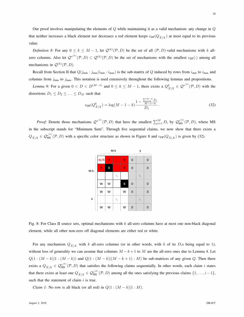
Definition 8: For any 0 ≤ k ≤ M − 1, let Q(k)(P, D) be the set of all (P, D)-valid mechanisms with k all-

zero columns. Also let Q∗(k)(P, D) ⊂ Q(k)(P, D) be the set of mechanisms with the smallest εDP(·) among all

mechanisms in Q(k)(P, D).

Recall from Section II that Q(jmin : jmax|imin : imax) is the sub-matrix of Q induced by rows from imin to imax and

columns from jmin to jmax. This notation is used extensively throughout the following lemmas and propositions.

Lemma 9: For a given 0 < D < D(M−1) and 0 ≤ k ≤ M − 1, there exists a QkX|X ∈ Q

∗(k)(P, D) with the

distortions D1 ≤ D2 ≤ . . . ≤ DM such that

εDP(QkX|X) = log(M − 1− k)

1−∑M−ki=2 DiM−1−kD1

. (32)

Proof: Denote those mechanisms Q∗(k)(P, D) that have the smallest∑Mi=1Di by Q∗(k)MS (P, D), where MS

in the subscript stands for “Minimum Sum”. Through five sequential claims, we now show that there exists a

QX|X ∈ Q∗(k)

MS (P, D) with a specific color structure as shown in Figure 8 and εDP(QX|X) is given by (32).

W/R R R 0 0

R B R 0 0

⋱ ⋱

W W B 0 0

W W W 0 0

⋱ ⋱

W W W 0 0

k M-k

M-k

k

Fig. 8: For Class II source sets, optimal mechanisms with k all-zero columns have at most one non-black diagonal

element, while all other non-zero off diagonal elements are either red or white.

For any mechanism QX|X with k all-zero columns (or in other words, with k of its Dis being equal to 1),

without loss of generality we can assume that columns M −k+ 1 to M are the all-zero ones due to Lemma 4. Let

Q(1 : (M − k)|1 : (M − k)) and Q(1 : (M − k)|(M − k + 1) : M) be sub-matrices of any given Q. Then there

exists a QX|X ∈ Q∗(k)

MS (P, D) that satisfies the following claims sequentially. In other words, each claim i states

that there exists at least one QX|X ∈ Q∗(k)

MS (P, D) among all the ones satisfying the previous claims {1, . . . , i−1},

such that the statement of claim i is true.

Claim 1: No row is all black (or all red) in Q(1 : (M − k)|1 : M).


21

Proof: Assume the contrary that the ith row in Q(1 : (M−k)|1 : M) is all black for any QX|X ∈ Q∗(k)

MS (P, D).

Consider the ratio εDP(Q) = log Q(1|i)Q(1|j) , where Q(1|j) is the red element associated with Q(1|i) which is black,

i.e. Q(1|j) and Q(1|i) form critical pairs. Also note that for any other 2 < l ≤ M − k, Q(l|i) ≥ Q(l|j). Now, if

εDP(Q) > 0, we have

1 = Q(1|i) +

M−k∑l=2

Q(l|i) > Q(1|j) +

M−k∑l=2

Q(l|j) = 1, (33)

which is a contradiction. Otherwise, if εDP(Q) = 0, by Lemma 7 D ≥ D(M−1), which is also a contradiction to our

assumption of 0 < D < D(M−1) in the beginning of converse proof. The proof for no row with all red elements

is similar.

Claim 2: All the off-diagonal elements of a row in Q(1 : (M − k)|1 : M) have the same color.

Proof: Take an arbitrary mechanism QX|X ∈ Q∗(k)

MS (P, D) that Q(1 : (M − k)|1 : M) satisfies Claim 1. Fix

a row i, and let the number of off-diagonal elements in row i of Q(1 : (M − k)|1 : M) with each of the colors

black, white and red be nB , nW and nR respectively, where nB + nW + nR = M − 1 − k. If only one of nR,

nW or nB is non-zero, then the claim is satisfied. We split the remaining scenarios into two cases and show that

in each it is sufficient to make all off-diagonal elements of the ith row white.

• If nR, nB > 0, then there exists an arbitrarily small δ > 0 such that each of the off-diagonal black elements can

be decreased by δnB

, and each of the off-diagonal red elements can be increased by δnR

. Consider a Q′ which

is identical to Q everywhere except for a segment of the i-th row Q′(1 : (M−k)|i). For 1 ≤ j ≤M−k, j 6= i,

let Q′(j|i) = Q(j|i) − δnB

if Q(j|i) is black, Q′(j|i) = Q(j|i) + δnR

if Q(j|i) is red, and Q′(j|i) = Q(j|i)

if Q(j|i) is white. Note that it does not matter if nW = 0 or not, because the white off-diagonal elements

Q′(1 : (M − k)|i) are not changed.

• If nR = 0, nW , nB > 0 (or nB = 0, nW , nR > 0), then there exists an arbitrarily small δ > 0 such that

each of off-diagonal white elements can be increased (or decreased) by δnW

, and each of off-diagonal black

elements (or red elements) can be decreased (or increased) by δnB

(or δnR

). Consider a Q′ which is identical

to Q everywhere except for Q′(1 : (M − k)|i). For 1 ≤ j ≤ M − k, j 6= i, let Q′(j|i) = Q(j|i) − δnB

if

Q(j|i) is black and Q′(j|i) = Q(j|i) + δnW

if Q(j|i) is white (or Q′(j|i) = Q(j|i) + δnR

if Q(j|i) is red and

Q′(j|i) = Q(j|i)− δnW

if Q(j|i) is white), and Q′(j|i) = Q(j|i) elsewhere.

In both cases Q′ has the same off-diagonal row sum and the same set of {Di}Mi=1 as Q, but for sufficiently small

δ, Q′ is still a valid row stochastic matrix and none of the elements in Q′(1 : (M −k)|1 : M) become 1 or 0. Thus,

Q′ would still be a (P, D)-valid mechanism. Besides, all off-diagonal elements in row i of Q′, i /∈ {a1, a2, · · · , ak},

are white: If not we would have a smaller εDP(Q′X|X) due to Remark 7, which contradicts our first assumption that

QX|X ∈ Qk∗(P, D). In this construction, all off-diagonal elements of Q′(1 : (M − k)|1 : M) in rows other than

i are colored the same as Q without affecting the average distortion, while keeping εDP(Q′) ≤ εDP(Q) and thus

Q′ ∈ Q∗(k)MS (P, D). This operation can be done for each row i repeatedly, to get the final Q′ to satisfy the claim.

Remark 8: As a result of Claims 1 and 2, all the off-diagonal elements in Q(1 : (M − k)|(M − k+ 1) : M) are

white.


22

Claim 3: If a diagonal element in Q(1 : (M − k)|1 : (M − k)) is not black then all off-diagonal elements of

Q(1 : (M − k)|1 : (M − k)) in the same row are red.

Proof: Take an arbitrary QX|X ∈ Q∗(k)

MS (P, D) satisfying Claims 1 and 2, and for some 1 ≤ i ≤M−k suppose

Q(i|i) is red or white. By Claim 2, all elements in the set {Q(j|i) : j 6= i, 1 ≤ j ≤ M − k} have the same color.

Assume to the contrary that they are not all red, so they are all black or white. Consider a Q′ which is equal to Q,

except in Q′(1 : (M − k)|i) where Q′(i|i) = Q(i|i) + δ and Q′(j|i) = Q(j|i)− δM−k−1 for j 6= i, 1 ≤ j ≤M − k.

For sufficiently small δ > 0 this is also a (P, D)-valid mechanism. Although εDP(Q′X|X) remains unchanged due

to Remark 7, we haveM∑i=1

D′i =

M∑i=1

(1−Q′(i|i)) <M∑i=1

(1−Q(i|i)) =

M∑i=1

Di, (34)

where D′i is the distortion of ith element under Q′. This clearly contradicts the assumption that Q ∈ Q∗(k)MS (P, D).

Claim 4: There is at most one non-black element on the diagonal of Q(1 : (M − k)|1 : (M − k)).


MS (P, D) satisfying all previous claims. Assume the contrary that there

are at least two non-black diagonal elements Q(i|i) and Q(j|j), (i 6= j, i, k ≤M−k). Thus, Q(i|j) is red by Claim

3, which implies that there exists a k 6= j where Q(i|k) is black, because there should be a black element for each

red element in a column. However, k 6= i because we already know that Q(i|i) is non-black. Thus, Q(i|k) has to

be an off-diagonal black element in Q(1 : (M − k)|1 : M), which is contradictory to our first assumption of Q

satisfying all previous claims, including Claim 1 and 2. Therefore, at most one diagonal element is non-black.

Claim 5: The only possible non-black element along the diagonal of Q(1 : (M − k)|1 : (M − k)) is the one

corresponding to the smallest, or one of the smallest Dis.


MS (P, D) satisfying all previous claims. Let the diagonal element in row

i, 1 ≤ i ≤ M − k, be non-black. We show that for any j 6= i, 1 ≤ j ≤ M − k, Dj ≥ Di. By Claim 3, we know

that any other off-diagonal entry in row i of Q(1 : (M − k)|1 : (M − k)), including Q(j|i) is red. We also know

that Q(j|j) is black and other entries in row j of Q(1 : (M − k)|1 : (M − k)), including Q(i|j), are either all

red or all white due to Claims 1 and 2. Thus, for all 1 ≤ k ≤M − k other than i or j we have Q(k|j) ≥ Q(k|i)

because Q(k|j) is either red or white, and Q(k|i) is red, where both of them are in the same column. Since any

row has to sum up to one, summing over rows i and j results in

Q(j|j) +Q(i|j) ≤ Q(i|i) +Q(j|i). (35)

Besides, since Q(j|j) is black, Q(j|i) is either red or white, Q(i|j) is red, and Q(i|i) is either red or white, we

haveQ(j|j)Q(j|i)

>Q(i|i)Q(i|j)

. (36)

We now show that

1− Dj = Q(j|j) ≤ Q(i|i) = 1− Di. (37)

Assume the contrary that Q(j|j) > Q(i|i). Thus, by (35) we have

0 < Q(j|j)−Q(i|i) ≤ Q(j|i)−Q(i|j), (38)


23

which means Q(j|j)−Q(i|i)Q(j|i)−Q(i|j) ≤ 1. However, (36) shows that

Q(j|j)−Q(i|i)Q(j|i)−Q(i|j)

≥ Q(j|j)Q(j|i)

>Q(i|i)Q(i|j)

≥ 0, (39)

which means

Q(j|j)−Q(i|i) > Q(j|i)−Q(i|j) (40)

because eεDP(Q) = Q(j|j)Q(j|i) > 1, which contradicts (38).

The claims above imply that for D1 as one of the smallest {Di}M−ki=1 , all the other diagonal elements are black,

and the non-zero elements in the row corresponding to D1 are all red. This implies that for each red Q(j|1), j 6= i,

there exists a diagonal element 1 −Dj in the same column j which is eεDP(Q) times bigger than the red element

Q(j|1). The proof is completed by summing over row 1 entries and solving for εDP.

Let 0 ≤ k ≤M −1. Lemma 9 provides a formula for the optimal εDP(·) among (P, D)-valid mechanisms with k

all-zero columns, in terms of their corresponding distortion values {Di}M−ki=1 . Besides, no mechanism with at least

k all-zero columns can be (P, D)-valid for D < D(k) due to Lemma 8. Thus, for any k and D(k) ≤ D ≤ D(k+1),

a lower bound on ε∗DP(P, D) can be derived by taking the minimum over 0 ≤ l ≤ k and all (P, D)-valid sets of

{Di}Mi=1 that satisfy (M −1−k)1−

∑M−ki=2

DiM−1−kD1

≥ 1, or equivalently∑M−ki=1 Di ≤M −1. Moreover, for a mechanism

with k all-zero columns we have Di = 1 for i > M − k, and thus {Di}Mi=1 can be (P, D)-valid if and only if

{Di}M−ki=1 is (P, D − D(k))-valid, i.e.∑M−ki=1 PiDi ≤ D − D(k). This result in (11) and completes the proof of

the lower bound in Theorem 2.

We now proceed to the special case where D < D(1). For proving ε∗DP(P, D) ≥ log(M − 1) 1−DD , it suffices to

show that ε∗(0)

DP (P, D) is greater than or equal to log(M − 1) 1−DD . We need the following Lemma.

Lemma 10: Let {ai}ni=1, {bi}ni=1, and {a′i}ni=1 be a collection of real numbers between 0 and 1, such thatn∑i=1

ai =

n∑i=1

a′i, (41)

and b1 ≤ b2 ≤ . . . ≤ bn. If a′1 ≥ a1 and a′i ≤ ai for i = 2, 3, · · · , n, thenn∑i=1

a′ibi ≤n∑i=1

aibi. (42)

Then, assume the contrary that for some D < D(1), all mechanisms in Q∗(P, D) achieve a strictly smaller

εDP(·) than log(M − 1) 1−DD . From Lemma 9 we know that there exists an optimal mechanism QX|X with the set

of distortions {Di}Mi=1, such that εDP(Q) is given by (32), and without loss of generality D1 ≤ D2 ≤ · · · ≤ DM

due to Lemma 4. Hence, the contrary assumption is that there exists an optimal QX|X such that

ε∗DP(Q, D) = εDP(QX|X) = log(M − 1)1−

∑Mi=2DiM−1D1

(43a)

< log(M − 1)1−DD

. (43b)

Thus:

(1−D)D1 +D

M − 1

M∑i=2

Di > D. (44)


24

On the other hand, since QX|X is supposed to satisfy the distortion constraint for any P ∈ P , including P ∗ =

argmaxP∈PPM , we have

M∑i=1

P ∗i Di = P ∗1D1 +

M∑i=2

P ∗i Di (45a)

= (1−D)D1 +D

M − 1

M∑i=2

Di ≤ D, (45b)

where (45b) is in view of Lemma 10 and the fact that D ≤ D(1) implies P ∗i ≥ DM−1 for i = 2, 3, · · · ,M and

P ∗1 ≤ 1−D. Obviously (45b) contradicts (44). Thus, for 0 ≤ D ≤ D(1), we have

ε∗DP(Q, D) ≥ log(M − 1)1−DD

. (46)

2) Achievability for Theorem 2: First, we show that for 0 ≤ D < D(1), the optimal leakage in (10) is achievable.

Consider the following mechanism

Q(j|i) =

1−D, i = j,

DM−1 , i 6= j.

(47)

Observe that Q is (P, D)-valid and εDP(Q) = log(M − 1) 1−DD . Therefore, the lower bound in (46) is tight and

ε∗DP(P, D) = log(M − 1) 1−DD for 0 ≤ D < D(1).

We now prove that the lower bound in (10) is achievable for D(1) ≤ D < D(M−1). To this end, we construct the

following mechanism. For any given 0 ≤ k ≤M − 1 and the optimal set {D∗i }M−1i=1 in (11), consider the following

mechanism.

Q(k)∗(j|i) =

1−D∗i , i = j ≤M − k,

Di1−D∗j∑l 6=i 1−D∗l

, i 6= j, i, j < M − k,

Q(k)∗(j|M − k), i > M − k, j ≤M − k,

0, j > M − k.

(48)

We now verify that εDP(Q(k)∗) = (M − 1− k)1−

∑M−ki=2

D∗iM−1−kD∗1

. Since each of the last k rows in the above matrix are

equal to the (M − k)th row, and the last k columns are all equal to zero, it suffices to check the εDP(·) for the

square matrix formed by the first M − k rows and columns. The ratio of any two elements in the same column in

Q(k)∗ belongs to the set {c1, c2, . . . , cM−k}, where

ci = (M − 1− k)1−

∑j 6=iDj

M−1−kDi

. (49)

From Lemma 4 we have that D1 ≤ . . . ≤ DM−k, which in turn implies that for any 0 ≤ j ≤M − k:

(M − 1− k)1−

∑M−ki=2 DiM−1−kD1

≥ (M − 1− k)1−

∑i6=j Di

M−1−kDj

. (50)

Therefore, εDP(Q(k)∗) = (M − 1− k)1−

∑M−ki=2

DiM−1−kD1

.


25

G. Proof of Theorem 3: Class III source sets

Proof: Recall that a Class III source set P can be written as a union of Class II source sets as P = ∪T∈TP

P|T .

Furthermore, each of these partitions P|T can be mapped to S0 with the appropriate permutation to get P|T . We

write the intersection and union of the mapped partitions as P∩ and P∪, respectively. Since P∩ and P∪ are Class

II source sets, we can compute the optimal leakage and the corresponding mechanism for these two sets. Moreover,

mapping P∪ and P∩ back into the original partitions results in two sets PUB and PLB that contain and are contained

in P , respectively.

Formally, let

PLB = ∪T∈TPT−1(P∩), (51a)

PUB = ∪T∈TPT−1(P∪). (51b)

For the P shown in Figure 2 and the corresponding P∪ and P∩ in Figure 3, Figure 9 below illustrates the PLB

and PUB.

P1

P3

P2𝒮0

𝑈𝐵

P1

P3

P2𝒮0

𝐿𝐵

Fig. 9: A source set P and its folded versions.

Recall that for two sets P1 and P2, if P1 ⊆ P2, then ε∗DP(P1, D) ≥ ε∗DP(P2, D). Thus, it suffices to show the

following:

(i) PLB ⊆ P ⊆ PUB, and

(ii) The optimal DP leakage for PLB and PUB are given by

ε∗DP(PLB, D) = ε∗DP:III(P∩, D, TP), (52)

ε∗DP(PUB, D) = ε∗DP:III(P∪, D, TP), (53)

where ε∗DP:III(·) is defined in (17).

Proof of (i): For each T ∈ TP , since P∩ ⊆ P|T we have T−1(P∩) ⊆ P|T . After taking union over all T ∈ TP ,

we have PLB ⊆ P . One can immediately show that P ⊆ PUB.

Proof of (ii): We first prove (52). A similar argument proves (53). Recall that PLB = ∪T∈TPT−1(P∩), and thus,

for any P ∈ P∩ and T ∈ TP we have T−1(P ) ∈ PLB. This means that for any given (PLB, D)-valid mechanism


26

QX|X , QT (X)|T (X) is also (PLB, D)-valid and εDP(QX|X) = εDP(QT (X)|T (X)). Since εDP(Q) is a quasi-convex

function of Q due to Lemma 1, there exists an optimal mechanism achieving ε∗DP(PLB, D) for which

DT (i) = Di, for any T ∈ TP , i = 1, . . . ,M. (54)

Hence, it suffices to search over only those (P∩, D)-valid mechanism that satisfy (54) in order to find ε(k)∗

DP (PLB, D).

Furthermore, since P∩ is a Class II source set, we can use the results from Theorem 2. We now show ε∗DP(PLB, D) =

ε∗DP:III(P∩, D, TP).

First consider the case where D ≥ M−1M . Clearly, choosing Q(i|j) = 1

M achieves ε∗DP(PLB, D) = 0, while the

distortion constraint is also satisfied.

For D < M−1M , similar to the proof for Theorem 2, we first restrict the set of mechanisms to those that have a

fixed number k of all-zero columns, k = 0, 1, . . . ,M − 1. For any such k, the optimal leakage is given by (18),

where the third constraint is a result of (54). Note that (18) results from the addition of the constraint in (54) to the

constraints in (11) for a Class II source set. The optimal ε∗DP(PLB, D) is then the minimum of ε(k)∗

DP:III(P∩, D, TP)

over all k, resulting in (17).

Finally, for D < D(1), analogous to Theorem 2, we can still show that the optimal mechanism is symmetric.

Recall that for a Class II source set P∩ and D < D(1), the optimal mechanism achieving ε∗DP(P∩, D) is symmetric,

and thus, does not violate (54). Hence, we have

ε∗DP:III(P∩, D, TP) = ε∗DP(P∩, D) = log

((M − 1)

1−DD

).

Note that in contrast to Theorem 2, we no longer have distortion thresholds D(2), D(3), . . . , D(M−2), where in

each of them only mechanisms with specific number of all-zero columns are allowed. This is due to the constraint

in (54), which may not allow a gradual shrinking of output support set.

VI. CONCLUSION

In this paper, we have quantified the privacy-utility tradeoffs for a dataset under different assumptions on

distribution knowledge (classes) and for Hamming distortion using differential privacy as the leakage metric. The

guarantees we can make under differential privacy are stronger than those under mutual information-based measures

of privacy leakage: DP leakage is lower bounded by MI leakage. We divide source sets into three classes. For Class

I the optimal mechanism is symmetric. For Class II achieving optimal leakage involves reducing the output space

as the distortion increases. For Class III sets we can use Class II results to develop upper and lower bounds on the

leakage.

Our results show that symmetric distortion, such as randomized response [27], is optimal when very little is

known about the source distribution or when the distortion requirement is very strict. In cases where the source

distribution is partially known, data publishers can take advantage of this to tailor a local privacy mechanism to

guarantee lower privacy leakage for the same distortion, or lower distortion for the same privacy leakage. These

gains can be significant if quite a lot is known about the source, such as Class II sources, and degrades as less


27

and less information is known. These results imply that domain knowledge or public data should be used when

designing mechanisms for publishing private data.

There are several interesting questions which we leave for future work. Obviously, a full characterization of

Class III sources would be welcome, but the techniques here should extend directly to general discrete distortion

measures (linear and nonlinear). Extensions to continuous source distributions may be trickier, but perhaps a starting

point would be distributions with bounded support. Finally, understanding the implications of this simple model to

categorical and hierarchically categorized data would help build insight into designing practical source-aware data

release mechanisms.

REFERENCES

[1] A. Sarwate and L. Sankar, “A rate-disortion [sic] perspective on local differential privacy,” in Proceedings of the 52nd Annual Allerton

Conference on Communication, Control and Computation (Allerton 2014), Sep. 2014, pp. 903–908.

[2] K. Kalantari, L. Sankar, and A. D. Sarwate, “Optimal differential privacy mechanisms under hamming distortion for structured source

classes,” in Proceedings of the 2016 IEEE International Symposium on Information Theory (ISIT), Jul. 2016, pp. 2069–2073.

[3] C. Dwork, F. McSherry, K. Nissim, and A. Smith, “Calibrating noise to sensitivity in private data analysis,” in Theory of Cryptography,

ser. Lecture Notes in Computer Science, S. Halevi and T. Rabin, Eds., vol. 3876. Berlin, Heidelberg: Springer, Mar. 2006, pp. 265–284.

[4] C. Dwork and A. Roth, “The algorithmic foundations of differential privacy,” Foundations and Trends in Theoretical Computer Science,

vol. 9, no. 3–4, pp. 211–407, Aug. 2014.

[5] A. D. Sarwate and K. Chaudhuri, “Signal processing and machine learning with differential privacy: theory, algorithms, and challenges,”

IEEE Signal Processing Magazine, vol. 30, no. 5, pp. 86–94, Sep. 2013.

[6] Q. Geng and P. Viswanath, “Optimal noise adding mechanisms for approximate differential privacy,” IEEE Transactions on Information

Theory, vol. 62, no. 2, pp. 952–969, Feb. 2016.

[7] L. Sankar, S. R. Rajagopalan, and H. V. Poor, “Utility-privacy tradeoffs in databases: An information-theoretic approach,” IEEE Transactions

on Information Forensics and Security, vol. 8, no. 6, pp. 838–852, Jun. 2013.

[8] F. du Pin Calmon and N. Fawaz, “Privacy against statistical inference,” in Proceedings of the 50th Annual Allerton Conference on

Communication, Control and Computation (Allerton 2012), Oct. 2012, pp. 1401–1408.

[9] D. Rebollo-Monedero, J. Forne, and J. Domingo-Ferrer, “From t-closeness-like privacy to postrandomization via information theory,” IEEE

Transactions on Knowledge and Data Engineering, vol. 22, no. 11, pp. 1623–1636, Nov. 2010.

[10] D. Agrawal and C. C. Aggarwal, “On the design and quantification of privacy preserving data mining algorithms,” in Proceedings of the

Twentieth ACM SIGMOD-SIGACT-SIGART Symposium on Principles of Database Systems, ser. PODS ’01. New York, NY, USA: ACM,

2001, pp. 247–255.

[11] H. Yamamoto, “A source coding problem for sources with additional outputs to keep secret from the receiver or wiretappers (corresp.),”

IEEE Transactions on Information Theory, vol. 29, no. 6, pp. 918–923, Nov. 1983.

[12] N. Takbiri, A. Houmansadr, D. L. Goeckel, and H. Pishro-Nik, “Limits of location privacy under anonymization and obfuscation,” in

International Symposium on Information Theory (ISIT). Aachen, Germany: IEEE, 2017, pp. 764–768.

[13] N. Takbiri, A. Houmansadr, D. Goeckel, and H. Pishro-Nik, “Fundamental limits of location privacy using anonymization,” in 51st Annual

Conference on Information Science and Systems (CISS). Baltimore, MD, USA: IEEE, 2017.

[14] N. Takbiri, A. Houmansadr, D. L. Goeckel, and H. Pishro-Nik, “Matching anonymized and obfuscated time series to users’ profiles,”

Available at https://arxiv.org/abs/1710.00197.

[15] M. S. Alvim, M. E. Andres, K. Chatzikokolakis, and C. Palamidessi, “On the relation between differential privacy and quantitative

information flow,” in Automata, Languages and Programming, L. Aceto, M. Henzinger, and J. Sgall, Eds. Berlin, Heidelberg: Springer

Berlin Heidelberg, 2011, pp. 60–76.

[16] M. S. Alvim, M. E. Andres, K. Chatzikokolakis, P. Degano, and C. Palamidessi, “Differential privacy: On the trade-off between utility

and information leakage,” in Formal Aspects of Security and Trust, G. Barthe, A. Datta, and S. Etalle, Eds. Berlin, Heidelberg: Springer

Berlin Heidelberg, 2012, pp. 39–54.


28

[17] Y. H. Liu, S. H. Lee, and A. Khisti, “Information-theoretic privacy in smart metering systems using cascaded rechargeable batteries,” IEEE

Signal Processing Letters, vol. 24, no. 3, pp. 314–318, Mar. 2017.

[18] S. Han, U. Topcu, and G. J. Pappas, “Event-based information-theoretic privacy: A case study of smart meters,” in 2016 American Control

Conference (ACC), Jul. 2016, pp. 2074–2079.

[19] O. Javidbakht and P. Venkitasubramaniam, “Differential privacy in networked data collection,” in 2016 Annual Conference on Information

Science and Systems (CISS), Mar. 2016, pp. 117–122.

[20] W. Wang, L. Ying, and J. Zhang, “On the relation between identifiability, differential privacy, and mutual-information privacy,” IEEE

Transactions on Information Theory, vol. 62, no. 9, pp. 5018–5029, Sep. 2016.

[21] I. Issa, S. Kamath, and A. B. Wagner, “An operational measure of information leakage,” in 2016 Annual Conference on Information Science

and Systems (CISS), Mar. 2016, pp. 234–239.

[22] P. Cuff and L. Yu, “Differential privacy as a mutual information constraint,” in Proceedings of the 2016 ACM SIGSAC Conference on

Computer and Communications Security, ser. CCS ’16. New York, NY, USA: ACM, 2016, pp. 43–54.

[23] F. du Pin Calmon, A. Makhdoumi, and M. Medard, “Fundamental limits of perfect privacy,” in Proceedings of the 2015 IEEE International

Symposium on Information Theory (ISIT), Jun. 2015, pp. 1796–1800.

[24] S. Asoodeh, M. Diaz, F. Alajaji, and T. Linder, “Information extraction under privacy constraints,” Information, vol. 7, no. 1, p. 15, Mar.

2016.

[25] Y. O. Basciftci, Y. Wang, and P. Ishwar, “On privacy-utility tradeoffs for constrained data release mechanisms,” in 2016 Information Theory

and Applications Workshop (ITA), Jan. 2016, pp. 1–6.

[26] K. Kalantari, O. Kosut, and L. Sankar, “On the fine asymptotics of information theoretic privacy,” in Proceedings of the 54th Annual

Allerton Conference on Communication, Control and Computation (Allerton 2016), Sep. 2016, pp. 532–539.

[27] S. L. Warner, “Randomized response: A survey technique for eliminating evasive answer bias,” Journal of the American Statistical

Association, vol. 60, no. 309, pp. 63–69, 1965.

[28] A. Evfimievski, J. Gehrke, and R. Srikant, “Limiting privacy breaches in privacy preserving data mining,” in Proceedings of the Twenty-

Second ACM SIGMOD-SIGACT-SIGART Symposium on Principles of Database Systems (PODS), ser. PODS ’03. New York, NY, USA:

ACM, 2003, pp. 211–222.

[29] S. P. Kasiviswanathan, H. K. Lee, K. Nissim, S. Raskhodnikova, and A. Smith, “What can we learn privately?” SIAM Journal on Computing,

vol. 40, no. 3, pp. 793–826, Jun. 2011.

[30] J. Duchi, M. Jordan, and M. Wainwright, “Local privacy and statistical minimax rates,” in Foundations of Computer Science (FOCS), 2013

IEEE 54th Annual Symposium on, Oct. 2013, pp. 429–438.

[31] A. Smith, A. Thakurta, and J. Upadhyay, “Is interaction necessary for distributed private learning?” in Proc. of the 2017 IEEE Symposium

on Security and Privacy, May 2017, pp. 58–77.

[32] P. Kairouz, S. Oh, and P. Viswanath, “Extremal mechanisms for local differential privacy,” Journal of Machine Learning Research, vol. 17,

no. 17, pp. 1–51, 2016.

[33] C. Dwork, “Differential privacy,” in Encyclopedia of Cryptography and Security, 2nd ed., H. C. A. van Tilborg and S. Jajodia, Eds.

Boston, MA: Springer US, 2011, pp. 338–340.

[34] S. Boyd and L. Vandenberghe, Convex Optimization. New York, NY, USA: Cambridge University Press, 2004.

[35] D.-Z. Du and P. M. Pardalos, Eds., Minimax and Applications, 2nd ed., ser. Nonconvex Optimization and Its Applications. Dordrecht:

Springer-Science+Business Media, 1995.


Robust Privacy-Utility Tradeoffs under Differential ...

Documents

Transcript of Robust Privacy-Utility Tradeoffs under Differential ...