Robust Optimization Model for Runway Configurations...

International Journal of Operations Research and Information Systems, 5(3), 1-26, July-September 2014 1

Copyright © 2014, IGI Global. Copying or distributing in print or electronic forms without written permission of IGI Global is prohibited.

ABSTRACTThe Runway Configuration Management problem governs what combinations of airport runways are in use at a given time for an airport or a collection of airports. Runway configurations (groupings of runways), operate under Runway Configuration Capacity Envelopes (RCCEs) which limit arrival and departure capacities. The RCCE identifies unique capacity constraints based on which runways are used for arrivals, departures, and their direction of travel. When switching between RCCEs, due to a change in weather conditions or a change in the demand pattern, a decrement in arrival and departure capacities is incurred during the transition. This paper reports computational experience with two distinct models—a robust optimization model that addresses uncertainty in the arrival demand, and a previously studied model that does not include uncertainty in any of the parameters. Test case scenarios are based on data from the John F. Kennedy international airport in New York.

Robust Optimization Model for Runway Configurations

ManagementRui Zhang, Department of Decision, Operations and Information Technologies, University of

Maryland, College Park, MD, USA

Rex Kincaid, Department of Mathematics, The College of William & Mary, Williamsburg, VA, USA

Keywords: Air Traffic, Airport Runway Configurations, Mixed Integer Programming, Robust Optimization

1. INTRODUCTION

The dynamics of a metroplex, a grouping of airports in close geographic proximity, are governed by a complex underlying framework of airport regulatory guidance, competition, and feasibility constraints. Efficiency is gaining increased importance in metroplex operations, since up to three times the current traffic demand for the U.S. national airspace is expected by 2025 (Technology Pathways, 2005; FAA and MITRE Corporation, 2007). Expanding existing or building new airports is not only an expensive

and time consuming task, but more critically it is often geographically infeasible due to space limitations in high demand city centers and urban areas. In order to alleviate conges-tion while maintaining connectivity to desired destinations, airport operations must be tuned as closely to optimal conditions as possible. More-over, future airspace management systems are likely to consolidate air transportation decisions at the metroplex rather than individual airports. Efficient operation of a metroplex introduces several challenging, dependent, sub-problems at each individual airport including, runway

DOI: 10.4018/ijoris.2014070101


2 International Journal of Operations Research and Information Systems, 5(3), 1-26, July-September 2014

configuration management (Provan and Atkins, 2010), surface operations (Tsao and Pratama, 2011), arrival and departure scheduling (Atkin, Burke, Greenwood and Reeson, 2008) and gate assignments (Das, 2009).

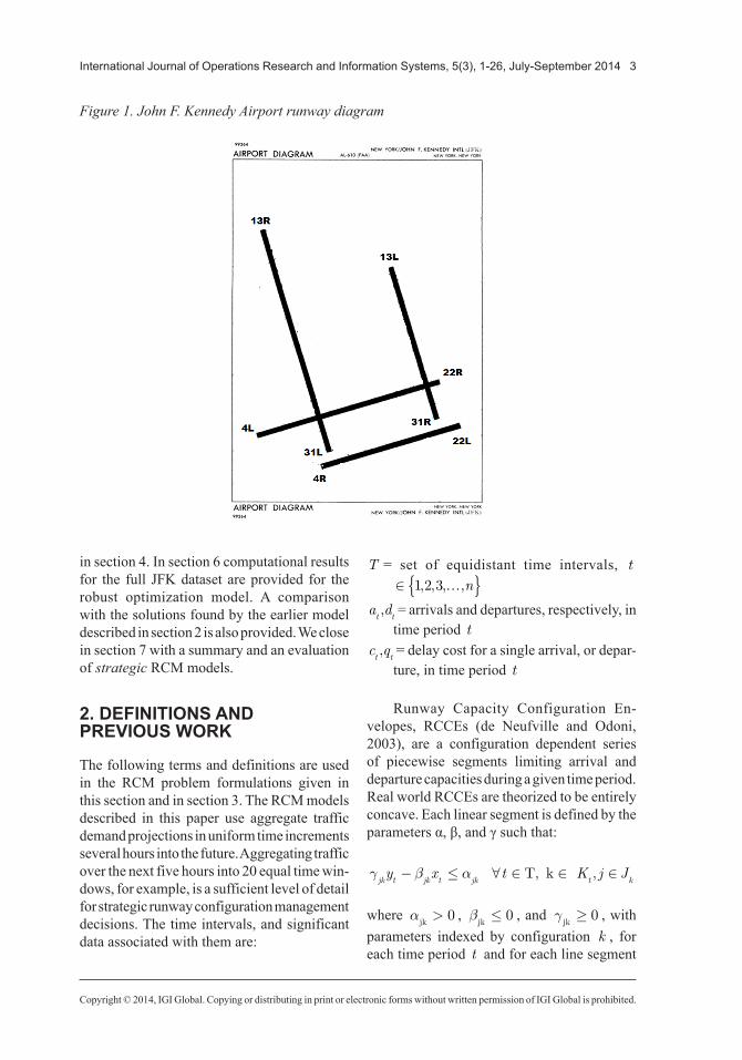
This paper addresses the Runway Configu-ration Management (RCM) problem. Air traffic controllers must make decisions regarding when to change from one configuration of runways to another. Runways are numbered between 01 and 36. Runway numbers are found by rounding one tenth of the magnetic azimuth of the runway’s heading. For example, a runway numbered 09 points east (85-95°). If there is more than one runway pointing in the same direction (parallel runways), each runway is identified by appending Left (L), Center (C) and Right (R) to the number. Figure 1 shows the FAA airport diagram for the John F. Kennedy (JFK) International airport. There are two pairs of orthogonal runways: 4L, 22R, 4R, 22L, 13R, 31L, 13L and 31R. Each runway may be used for arrivals only, departures only, or a mixed arrival and departure pattern. For example, 31R | 31L, is a runway configuration in which 31R is used only for arrivals and 31L is used only for departures. Usually, runways before “|” are used for arrivals and those after it are for departures.

We call an RCM problem strategic if the planning window is five hours or more and tactical if the planning window is less than five hours. The tactical RCM problem requires detailed information about each planned arrival and departure in the time window and does not lend itself to a closed form performance metric. Thorne and Kincaid (2012) describe a heuristic search procedure for the tactical RCM problem that relies on a scenario based Monte Carlo simulation to evaluate each proposed configuration change. The focus in this paper is the strategic RCM problem in which the use of aggregate arrival and departure information leads to a closed form performance metric. For a five hour planning time scale, determining when to change from one runway configuration to another does not require detailed information of individual flights. Instead, aggregate arrival

and departure demand is sufficient. There are two reasons for this. First, cumulative overall system performance rather than individual flight performance is the objective of interest in strategic RCM. Second, system uncertainties prohibit a fine level of detail for future planning. Hereafter, when we refer to the RCM problem we mean the strategic RCM problem.

Changing runway configurations impacts airport arrival and departure capacities since each runway configuration has a different RCCE. Determining when to change from one configuration to another is complicated by a dynamic system rich with uncertainty. It is therefore not possible to deterministically forecast configurations in which to operate throughout the day. Weather conditions such as wind speed, wind direction, and cloud cover ceiling are among the most influential charac-teristics governing configurations available for use. The demand for aircraft arrivals and departures in each time period further limits the number of feasible configurations. Additionally, environmental constraints such as noise and no-fly restrictions over populated areas are often present at varying times of the day. Regardless of the system’s dynamic nature, the ability to generate a schedule of configuration changes is essential. RCM models are an attempt to provide air traffic controllers with a tool to assist in the scheduling of configuration changes. The main goal of this paper is to develop an RCM model that provides a mechanism for address-ing uncertainty in the arrival demand in each planning time period.

The paper is organized as follows. In section 2 key terms and definitions needed to describe the optimization models for RCM are provided as well as a summary of a previous RCM model (Weld, Duarte, and Kincaid, 2010). This model is extended in section 3 by adding uncertainty to the arrival demand in all planning time periods via a robust optimization approach. Section 4 contains a description of how our computational experiments are conducted. A small example is provided in section 5 to illustrate both the robust optimization model described in section 3 and the computational experiment procedure



in section 4. In section 6 computational results for the full JFK dataset are provided for the robust optimization model. A comparison with the solutions found by the earlier model described in section 2 is also provided. We close in section 7 with a summary and an evaluation of strategic RCM models.

2. DEFINITIONS AND PREVIOUS WORK

The following terms and definitions are used in the RCM problem formulations given in this section and in section 3. The RCM models described in this paper use aggregate traffic demand projections in uniform time increments several hours into the future. Aggregating traffic over the next five hours into 20 equal time win-dows, for example, is a sufficient level of detail for strategic runway configuration management decisions. The time intervals, and significant data associated with them are:

T = set of equidistant time intervals, t∈ …{ }1 2 3, , , ,n

a dt t, = arrivals and departures, respectively, in

time period t c qt t, = delay cost for a single arrival, or depar-

ture, in time period t

Runway Capacity Configuration En-velopes, RCCEs (de Neufville and Odoni, 2003), are a configuration dependent series of piecewise segments limiting arrival and departure capacities during a given time period. Real world RCCEs are theorized to be entirely concave. Each linear segment is defined by the parameters α, β, and γ such that:

γ β αjk t jk t jk t ky x t K j J− ≤ ∀ ∈ ∈ ∈�� , ,�T��k �

where αjk> 0 , β

jk≤ 0 , and γ

jk≥ 0 , with

parameters indexed by configuration k , for each time period t and for each line segment

Figure 1. John F. Kennedy Airport runway diagram



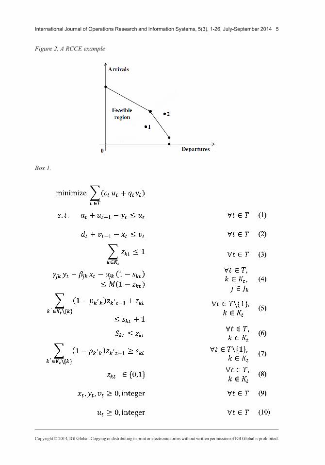
j . Figure 2 is an example of RCCE with three linear segments describing the capacity for arrivals and departures of a runway configura-tion in one time period. The horizontal and vertical axes express departure capacity and arrival capacity respectively. The points labeled 1 and 2 are examples of two demand patterns. Point 1 is satisfied by this runway configuration, but point 2 is not. Consequently, another con-figuration is needed to satisfy the arrival and departure demand represented by point 2. This idea allows for a straightforward series of linear constraints to approximate RCCEs within our optimization model through a combination of piecewise linear segments. Availability of configurations and their associated RCCEs are modeled by a set of binary integer variables. If the RCCE is active, the binary variable z

ktfor

configuration k , in time period t is set to 1. Additional variables x y u

t t t, , and v

t, are also

required to model met and unmet demand:

K = s e t o f a l l c o n f i g u r a t i o n s , k m� � ,� ,� ,� ,�∈ …{ }1 2 3

Kt= set of all configurations available in time period t

zkt=

1if configuration k is chosen in time period t

othe0 rrwise

(yt, xt) = number of arrival, y , and departure,

x , demand met in time period t (ut, vt) = unmet arrival, u , and departure, v ,

demand in time period t Jk

= set of RCCE line segments available for configuration k

More detailed information concerning RCCEs can be found in Weld, Duarte and Kincaid (2010).

The initial mathematical programming model for an RCM problem was given by Bertsimas, Frankovich and Odoni (2009). Weld, Duarte, and Kincaid (2010) proposed a margin-ally decreased transition capacity (MDTC)

model which extends the Bertsimas, Frankov-ich and Odoni(2009) model to cover more general situations. Two significant adjustments are made to the Bertsimas, Frankovich and Odoni(2009) model to achieve this goal. The first is a conceptual change, in which all RCCE subsets of any configuration are now referenced as their own unique configuration. The second adjustment comes by introducing a penalty matrix, P . Each entry, p

ij, of the penalty

matrix captures the decremented capacity inher-ent when switching between configuration i and configuration j . The robust optimization model developed in the next section is derived from the MDTC model given below.

The parameters p c q aij t t t, ,

, and d

t and the

decision variables x y u vt t t t, ,

, and z

kt are defined

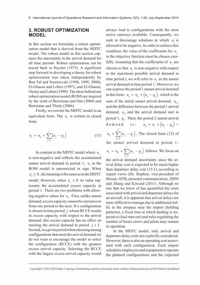
in the previous section. The parameter M is a suitably chosen large value. The objective func-tion (1) aims to minimize the weighted total of unmet arrival and departure demand experi-enced through runway configuration (equiva-lently RCCE) selections over all time periods. We note that u v

0 00= = . Constraints (2) and

(3) ensure conservation of demand (i.e. demand at t , plus carryover demand from t −1 , minus demand satisfied at t , does not exceed unmet demand for t ) for arrivals and departures, re-spectively. Constraint (4) ensures at most one configuration is selected for each time interval. Constraint (5) defines the appropriate RCCE, while constraints (6) through (8) describe the switching cost incurred by transitioning to configuration k at time t . The variable s

kt =

1− pij�if configuration j is switched from

configuration i at time t (and 0 otherwise) captures the cost of switching to configuration k at time t . When a configuration change is made, constraints (6), (7), and (8) assign s

kt a

value between 0 and 1 which is then used to decrease the frontier represented by constraint (5). The interested reader is referred to Weld, Duarte, and Kincaid (2010) for a detailed de-scription of the MDTC model (Box 1).



Figure 2. A RCCE example

Box 1.



3. ROBUST OPTIMIZATION MODEL

In this section we formulate a robust optimi-zation model that is derived from the MDTC model. The robust model in this section cap-tures the uncertainty in the arrival demand for all time periods. Robust optimization can be traced back to Soyster (1973). A significant step forward in developing a theory for robust optimization was taken independently by Ben-Tal and Nemirovski (1998, 1999, 2000), El-Ghaoui and Lebret (1997), and El-Ghaoui, Oustry and Lebret (1998). The ideas behind our robust optimization model (ROM) are inspired by the work of Bertsimas and Sim (2004) and Bertsimas and Thiele (2006).

Firstly, we rewrite the MDTC model in an equivalent form. The u

t is written in closed

form:

u u a yt

j

t

j j= + −( )

=∑0

1

(11)

In contrast to the MDTC model where ut

is non-negative and reflects the accumulated unmet arrival demand in period t , u

t in the

ROM model is unrestricted in sign. When ut�≥ 0 , the meaning is the same as in the MDTC

model. However, when ut< 0 its value rep-

resents the accumulated excess capacity in period t . There are two problems with allow-ing negative values for u

t. First, unlike unmet

demand, excess capacity cannot be carried over from one period to the next. If a configuration is chosen in time period j whose RCCE results in excess capacity, with respect to the arrival demand, this excess capacity has no effect on meeting the arrival demand in period j +1. Second, in a given period when choosing among configurations that meet the arrival demand we do not want to encourage the model to select the configuration (RCCE) with the greatest excess arrival capacity. Selecting the RCCE with the largest excess arrival capacity would

always lead to configurations with the most active runways available. Consequently, we seek to discourage solutions in which u

t is

allowed to be negative. In order to enforce this condition, the value of the coefficients for u

t

in the objective function must be chosen care-fully. Assuming that the coefficients of u

t are

chosen so that ut is non-negative with respect

to the maximum possible arrival demand in time period t, we will refer to u

t as the unmet

arrival demand at time period t . Moreover, we can express the period 1 unmet arrival demand in this form: u u a y

1 0 1 1= + −( ) , which is the

sum of the initial unmet arrival demand, u0

, and the difference between the period 1 arrival demand, a

1, and the arrival demand met in

period 1, y1. Then, the period 2 unmet arrival

d e m a n d i s : u u a y2 1 2 2= + −( ) =

�u a yj

j j01

2

+ −( )=∑ . The closed form (12) of

the unmet arrival demand at period t :

u u a yt

j

t

j j= + −( )

=∑0

1

follows. We focus on

the arrival demand uncertainty since the ar-rival delay cost is expected to be much higher than departure delay cost (15:1), according to expert views (Dr. Stephen, vice-president of Mosaic ATM, personal communication, 2009) and Zhang and Kincaid (2011). Although no one that we know of has quantified the costs associated with arrival and departure delays for an aircraft, it is apparent that arrival delays are more difficult to manage due to additional traf-fic in the airspace near the airport (holding patterns), a fixed time at which landing is im-perative (fuel runs out) and rules regulating the number of hours crews and pilots may remain in operation.

In the MDTC model, only arrival and departure delay costs are explicitly considered. However, there is also an operating cost associ-ated with each configuration. Each airport schedules employees and equipment to operate the planned configurations and the expected



demand. For our purposes, we consider the operating cost to be determined by the number of runways used in a configuration. Further-more, by introducing an operating cost, we are able to address a difficulty presented by our robust model. Without an operating cost in-cluded in our robust model, the configuration with largest capacity is always preferred. Next, we give a modified MDTC model with an operating cost, o

kt, and a new decision variable

At.

Let At denote the decision variable for the

arrival delay cost at time period t and let the operation cost be denoted by o

kt for each con-

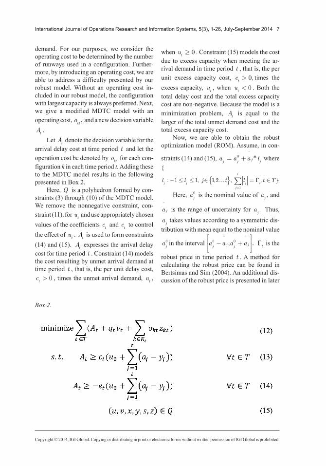
figuration k in each time period t. Adding these to the MDTC model results in the following presented in Box 2.

Here, Q is a polyhedron formed by con-straints (3) through (10) of the MDTC model. We remove the nonnegative constraint, con-straint (11), for u

t and use appropriately chosen

values of the coefficients ct and e

t to control

the effect of ut. A

t is used to form constraints

(14) and (15). At expresses the arrival delay

cost for time period t . Constraint (14) models the cost resulting by unmet arrival demand at time period t , that is, the per unit delay cost, ct> 0 , times the unmet arrival demand, u

t,

when ut≥ 0 . Constraint (15) models the cost

due to excess capacity when meeting the ar-rival demand in time period t , that is, the per unit excess capacity cost, e

t> 0, times the

excess capacity, ut, when u

t< 0 . Both the

total delay cost and the total excess capacity cost are non-negative. Because the model is a minimization problem, A

t is equal to the

larger of the total unmet demand cost and the total excess capacity cost.

Now, we are able to obtain the robust optimization model (ROM). Assume, in con-

straints (14) and (15), a a a lj j j j= +0

�

* where {

l l j t l t Tj j

j

t

j t: , , , , }− ≤ ≤ ∈ …{ } = ∈

=∑1 1 1 2

1

Γ .

Here, aj0 is the nominal value of a

j, and

a j�

is the range of uncertainty for aj. Thus,

aj takes values according to a symmetric dis-

tribution with mean equal to the nominal value

aj �0 in the interval a a a a

j j j j0 0− +

� �

, . Γt is the

robust price in time period t . A method for calculating the robust price can be found in Bertsimas and Sim (2004). An additional dis-cussion of the robust price is presented in later

Box 2.



section. Γt balances the robustness of ROM

against the level of acceptable uncertainty in the solution. Γ

t is increasing when t is increas-

ing and is increased by at most 1 for each time period. It is clear that in time period t, there are at most Γ

t coefficients changing with the

bound and one coefficient change within the range ( )Γ Γ

t t− . The resulting additions yield

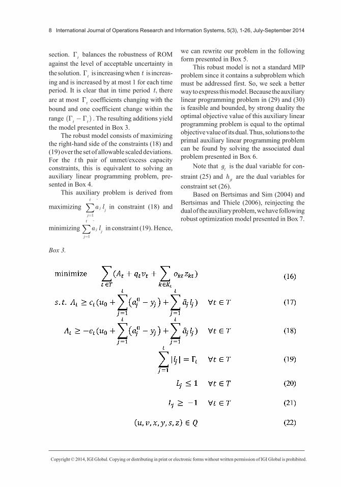
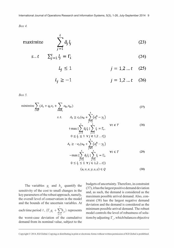
the model presented in Box 3.The robust model consists of maximizing

the right-hand side of the constraints (18) and (19) over the set of allowable scaled deviations. For the t th pair of unmet/excess capacity constraints, this is equivalent to solving an auxiliary linear programming problem, pre-sented in Box 4.

This auxiliary problem is derived from

maximizing j

t

j ja l

=∑

1

�

�in constraint (18) and

minimizing j

t

j ja l

=∑

1

�

�in constraint (19). Hence,

we can rewrite our problem in the following form presented in Box 5.

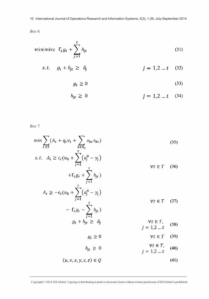
This robust model is not a standard MIP problem since it contains a subproblem which must be addressed first. So, we seek a better way to express this model. Because the auxiliary linear programming problem in (29) and (30) is feasible and bounded, by strong duality the optimal objective value of this auxiliary linear programming problem is equal to the optimal objective value of its dual. Thus, solutions to the primal auxiliary linear programming problem can be found by solving the associated dual problem presented in Box 6.

Note that gt is the dual variable for con-

straint (25) and hjt

are the dual variables for constraint set (26).

Based on Bertsimas and Sim (2004) and Bertsimas and Thiele (2006), reinjecting the dual of the auxiliary problem, we have following robust optimization model presented in Box 7.

Box 3.



The variables gt and h

jt quantify the

sensitivity of the cost to small changes in the key parameters of the robust approach, namely, the overall level of conservatism in the model and the bounds of the uncertain variables. At

each time period t , ( )Γt t

k

t

jtg h+

=∑

1

represents

the worst-case deviation of the cumulative demand from its nominal value, subject to the

budgets of uncertainty. Therefore, in constraint (37), it has the largest positive demand deviation and, as such, the demand is considered as the maximum possible arrival demand. Also, con-straint (38) has the largest negative demand deviation and the demand is considered as the minimum possible arrival demand. The robust model controls the level of robustness of solu-tions by adjusting Γ

t, which balances objective

Box 4.

Box 5.



Box 6.

Box 7.



performance and uncertainty. Alternatively, (37) and (38) in the robust model can be viewed as chance constraints, as described in Ben-Tal and Nemirovski (1998, 1999, 2000), Γ

t is selected

so that the desired probability of a constraint violation due to the uncertain parameters is achieved. We note that although we have focused exclusively on arrival demand uncertainty, the model is easily extended to address departure demand uncertainty.

Furthermore, we notice that in our model that the unmet demand cost in constraint (37) should not be tight (not satisfied as equality). The unmet demand cost modeled in constraint (37), should be less restrictive than constraint (38). The reason for this is that constraint (37) models the capacity to serve the maximum possible arrival demand and, as we have previ-ously noted, the excess capacity of serving arrival demand in any time period cannot be accumulated for use in later time periods. Therefore, e

t should be positive and much

smaller than ct, 0 < <<e c

t t, to ensure that

u u a y g ht

j

t

j j t tj

t

jt= + −( )+ +

= =∑ ∑0

1

0

1

Γ

is nonnegative in the constraints (38), meaning that u

t denotes the unmet arrival demand with

respect to the maximum possible arrival de-mand. Both constraints (37) and (38), derived from constraints (14) and (15) respectively, are necessary. When �0 < <<e c

t t, constraint (37)

pushes the model to have higher capacity so that the arrival demand is satisfied. On the other hand, constraint (38) prevents the model from acquiring unnecessary capacity. Thus, the model balances these conflicting goals and allocates resources accordingly.

4. EXPERIMENTAL PROCEDURE AND ENVIRONMENT

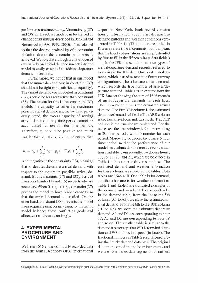
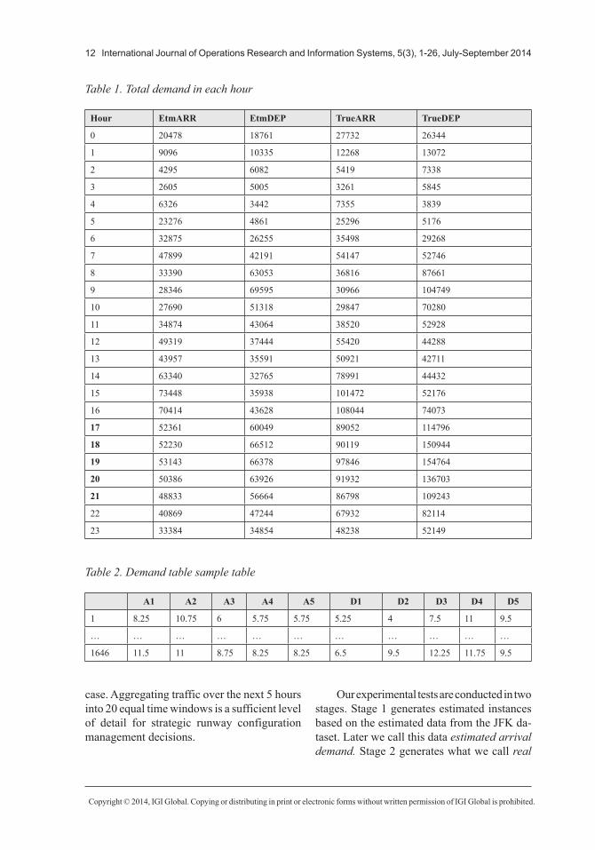
We have 1646 entries of hourly recorded data from the John F. Kennedy (JFK) international

airport in New York. Each record contains hourly information about arrival/departure demand patterns and weather conditions (pre-sented in Table 1). (The data are recorded in fifteen minute time increments, but it appears that the hourly observations are simply divided by four to fill in the fifteen minute data fields.)

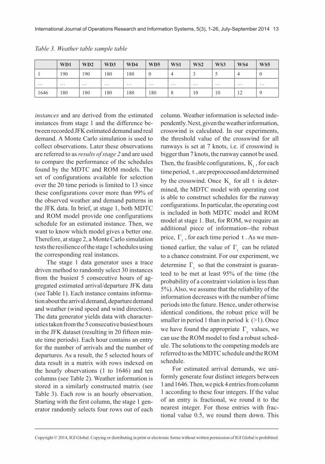
In the JFK dataset, there are two types of arrival/departure demand records, referred to as entries in the JFK data. One is estimated de-mand, which is used to schedule future runway configurations. The other one is real demand, which records the true number of arrival/de-parture demand. Table 1 is an excerpt from the JFK data set showing the sum of 1646 records of arrival/departure demands in each hour. The EtmARR column is the estimated arrival demand. The EtmDEP column is the estimated departure demand, while the TrueARR column is the true arrival demand. Lastly, the TrueDEP column is the true departure demand. For the test cases, the time window is 5 hours resulting in 20 time periods, with 15 minutes for each period. Moreover, we choose the busiest 5 hour time period so that the performance of our models is evaluated in the most extreme situa-tion available. Consequently, we choose hours, 17, 18, 19, 20, and 21, which are boldfaced in Table 1 to be our trace driven sample set. The estimated demand and weather information for these 5 hours are stored in two tables. Both tables are 1646 ×10. One table is for demand, and the other one is for weather information. Table 2 and Table 3 are truncated examples of the demand and weather tables respectively. In the demand table, from the 1st to the 5th column (A1 to A5), we store the estimated ar-rival demand. From the 6th to the 10th column (D1 to D5), we store the estimated departure demand. A1 and D1 are corresponding to hour 17; A2 and D2 are corresponding to hour 18 and so on. The weather table is similar to the demand table except that WD is for wind direc-tion and WS is for wind speed (in knots). The fractional numbers in Table 2 result from divid-ing the hourly demand data by 4. The original data are recorded in one hour increments and we use 15 minutes data segments for out test



case. Aggregating traffic over the next 5 hours into 20 equal time windows is a sufficient level of detail for strategic runway configuration management decisions.

Our experimental tests are conducted in two stages. Stage 1 generates estimated instances based on the estimated data from the JFK da-taset. Later we call this data estimated arrival demand. Stage 2 generates what we call real

Table 1. Total demand in each hour

Hour EtmARR EtmDEP TrueARR TrueDEP

0 20478 18761 27732 26344

1 9096 10335 12268 13072

2 4295 6082 5419 7338

3 2605 5005 3261 5845

4 6326 3442 7355 3839

5 23276 4861 25296 5176

6 32875 26255 35498 29268

7 47899 42191 54147 52746

8 33390 63053 36816 87661

9 28346 69595 30966 104749

10 27690 51318 29847 70280

11 34874 43064 38520 52928

12 49319 37444 55420 44288

13 43957 35591 50921 42711

14 63340 32765 78991 44432

15 73448 35938 101472 52176

16 70414 43628 108044 74073

17 52361 60049 89052 114796

18 52230 66512 90119 150944

19 53143 66378 97846 154764

20 50386 63926 91932 136703

21 48833 56664 86798 109243

22 40869 47244 67932 82114

23 33384 34854 48238 52149

Table 2. Demand table sample table

A1 A2 A3 A4 A5 D1 D2 D3 D4 D5

1 8.25 10.75 6 5.75 5.75 5.25 4 7.5 11 9.5

… … … … … … … … … … …

1646 11.5 11 8.75 8.25 8.25 6.5 9.5 12.25 11.75 9.5



instances and are derived from the estimated instances from stage 1 and the difference be-tween recorded JFK estimated demand and real demand. A Monte Carlo simulation is used to collect observations. Later these observations are referred to as results of stage 2 and are used to compare the performance of the schedules found by the MDTC and ROM models. The set of configurations available for selection over the 20 time periods is limited to 13 since these configurations cover more than 99% of the observed weather and demand patterns in the JFK data. In brief, at stage 1, both MDTC and ROM model provide one configurations schedule for an estimated instance. Then, we want to know which model gives a better one. Therefore, at stage 2, a Monte Carlo simulation tests the resilience of the stage 1 schedules using the corresponding real instances.

The stage 1 data generator uses a trace driven method to randomly select 30 instances from the busiest 5 consecutive hours of ag-gregated estimated arrival/departure JFK data (see Table 1). Each instance contains informa-tion about the arrival demand, departure demand and weather (wind speed and wind direction). The data generator yields data with character-istics taken from the 5 consecutive busiest hours in the JFK dataset (resulting in 20 fifteen min-ute time periods). Each hour contains an entry for the number of arrivals and the number of departures. As a result, the 5 selected hours of data result in a matrix with rows indexed on the hourly observations (1 to 1646) and ten columns (see Table 2). Weather information is stored in a similarly constructed matrix (see Table 3). Each row is an hourly observation. Starting with the first column, the stage 1 gen-erator randomly selects four rows out of each

column. Weather information is selected inde-pendently. Next, given the weather information, crosswind is calculated. In our experiments, the threshold value of the crosswind for all runways is set at 7 knots, i.e. if crosswind is bigger than 7 knots, the runway cannot be used. Then, the feasible configurations, K

t, for each

time period, t , are preprocessed and determined by the crosswind. Once K

t for all t is deter-

mined, the MDTC model with operating cost is able to construct schedules for the runway configurations. In particular, the operating cost is included in both MDTC model and ROM model at stage 1. But, for ROM, we require an additional piece of information--the robust price, Γ

t, for each time period t . As we men-

tioned earlier, the value of Γt can be related

to a chance constraint. For our experiment, we determine Γ

t so that the constraint is guaran-

teed to be met at least 95% of the time (the probability of a constraint violation is less than 5%). Also, we assume that the reliability of the information decreases with the number of time periods into the future. Hence, under otherwise identical conditions, the robust price will be smaller in period 1 than in period k (>1). Once we have found the appropriate Γ

t values, we

can use the ROM model to find a robust sched-ule. The solutions to the competing models are referred to as the MDTC schedule and the ROM schedule.

For estimated arrival demands, we uni-formly generate four distinct integers between 1 and 1646. Then, we pick 4 entries from column 1 according to these four integers. If the value of an entry is fractional, we round it to the nearest integer. For those entries with frac-tional value 0.5, we round them down. This

Table 3. Weather table sample table

WD1 WD2 WD3 WD4 WD5 WS1 WS2 WS3 WS4 WS5

1 190 190 180 180 0 4 3 5 4 0

… … … … … … … … … … …

1646 180 180 180 180 180 8 10 10 12 9



process is repeated to draw data from columns 2 through 5. The resulting 20 entries are our estimated arrival demands. For estimated de-parture demands, the procedure is the same except that we use columns 6 through column 10 from the demand table. Next, we draw weather information from the weather table. To do this, generate an integer, i , uniformly be-tween 1 and 1646. Then, for row i of the weather table, columns 1 to 5 give the wind direction for our 5 hour time interval. Columns 6 to 10 are the wind speed for our 5 hour time interval.

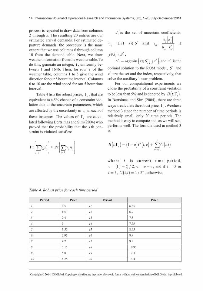
Table 4 lists the robust prices, Γt, that are

equivalent to a 5% chance of a constraint vio-lation due to the uncertain parameters, which are affected by the uncertainty in a

t in each of

these instances. The values of Γt are calcu-

lated following Bertsimas and Sim (2004) who proved that the probability that the i th con-straint is violated satisfies:

Pr Prjij j

j Jij ij

b xi

∑ ∑

≤

∈

* γ η

Ji is the set of uncertain coefficients,

γij= 1�i f j S∈ * and γ

ij

ij j

iã ã

b x

b x=�

*

** *

i f

j J Si i

� � \ *∈ ,

γ* * *= ∈{ }∪argmin r S ti i

and x * is the

optimal solution to the ROM model, S * and t * are the set and the index, respectively, that solve the auxiliary linear problem.

For our computational experiments we chose the probability of a constraint violation to be less than 5% and is denoted by B t

t,Γ( ) .

In Bertsimas and Sim (2004), there are three ways to calculate the robust price, Γ

t. We chose

method 3 since the number of time periods is relatively small, only 20 time periods. The method is easy to compute and, as we will see, performs well. The formula used in method 3 is:

B t u C t v C t lt

l v

t

, , ,Γ( ) = −( ) ( )+ ( )= +∑1

1

where t i s cu r ren t t ime pe r iod , v t u v v

t= + = −( ) / ,Γ 2 , and if l = 0 or l t= , C t l n, /( ) = 1 2 , otherwise,

Table 4. Robust price for each time period

Period Price Period Price

1 0.5 11 6.85

2 1.5 12 6.9

3 2.4 13 7.3

4 3 14 7.75

5 3.55 15 8.65

6 3.95 16 8.9

7 4.7 17 9.9

8 5.15 18 10.95

9 5.8 19 12.3

10 6.25 20 14.4



c t l

t

t l l

tt

t l

lt

l

,

exp* log

* log

( ) =

−( )−( )

+

−

1

2

2

1π

.

For t = 20 , the computed value of Γ = 14 4. . Then, to ensure that the constraint violation probability of 5% is met requires that only 14 4 20 72. / %≅ of the uncertain data be covered. But for constraints with fewer uncer-tain data, for example when t = 2 , the com-puted value of �Γ = 2 . This is too strong for our model because our model includes time transitivity. Therefore, we assume that the reli-ability of the information decreases as the number of time periods increase. Hence, in the earlier time periods, (e.g. t = 2 ) the robust price in Table 4 is smaller than the value com-puted by method 3. This means that the uncer-tainty of the parameters lie in relatively nar-rower ranges.

At Stage 2, 10 real instances are generated from each of the stage 1estimated instances. After compare the difference between the es-timated demand records and their correspond-ing real demand records in JFK data, we use the following method to generate “real” demand values: (1) For the arrival demand, RA EA Z= + +( )� � * � . � � . �* ,2 0 27 0 969 where Z is a standard normal variate, RA is the real arrival demand, and EA is the estimated ar-rival demand. (2) For the departure demand, RD ED Z= + +( )� � * . � � . *� ,2 0 0534 0 902 where the Z is a standard normal variate, RD is the real arrival demand, and ED is the estimated arrival demand. In these two steps, parameters, 2, 0.27, 0.969, 0.0534 and 0.902, and the normal distribution are derived from the difference between estimated demand records and their corresponding real demand records in the JFK data. (3) After we obtain RA or RD , we round any fractional part (up or down with equal probability) yielding integer values for RA and

RD. For each time period’s demand, the above equations are used to calculate the correspond-ing real demand. A Monte Carlo simulation is used to evaluate the performance of these two models. In the simulation, the MDTC and ROM schedules are used to satisfy real arrival/depar-ture demands. Hence, at stage 2, the configura-tions are fixed based on its corresponding the MDTC schedule and ROM schedule from stage 1 for each stage 2 real instance. Then, real in-stances data are plugged in MDTC model for the Monte Carlo simulation. Here, the MDTC model does not include the operating cost be-cause the configurations are fixed based on stage 1 results.

The cost parameter values in the MDTC and ROM models are difficult to estimate. Actual cost data for arrival delays and departure delays, as well as the operating cost a given configuration, are not readily available. Instead we use relative costs following expert views (Dr. Stephen Atkins, vice-president of Mosaic ATM, personal communication, 2009). As discussed in section 3, the arrival delay cost is assumed to be 15 times larger than the departure delay cost. Consequently, we set c

t= 15 and

gt= 15 . To enforce the nonnegative constraint

on ut, we need 0 < e c

t t� . In our tests,

e ct t= 0 2. * is used in each time period.

Similarly, the operating cost estimates are given relative to the number of runways. Thus, the operating cost of a configuration with two runways is 5. The operating cost for a three runway configuration is 7.5 while a four runway configuration is 10. That is, we assume addi-tional effort is needed to manage a configuration with more active runways according to expert views (Dr. Stephen Atkins, vice-president of Mosaic ATM, personal communication, 2009).

Both the MDTC and ROM models are written in AMPL and solved with Gurobi 2.0. All tests ran on machines which have 2 Opteron 2.6 GHz, dual-core processors, 20 GB RAM. Relative mixed integer optimality gaps of 0.01, 0.02 and 0.05 were used in the computational experiments.



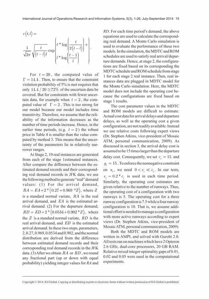
5. ROM EXAMPLE AND THE COMPUTATIONAL APPROACH

Here, we use a toy example to illustrate our models and computational experiments. In this example, we assume there are four time periods and three available configurations. Also, we ignore weather effects. Thus, any of the three configurations may be used in any time period. The arrival delay cost, c

t, is 15 and the depar-

ture cost, qt, is 1. A penalty cost to transition

between configurations of 10% of the original

RCCE capacity is used. For the ROM, ak�

, the varied range of uncertainty of a

k, is 4. The

operating cost of a configuration is chosen as 5, 7.5, and 10 for two, three and four runways respectively in this example.

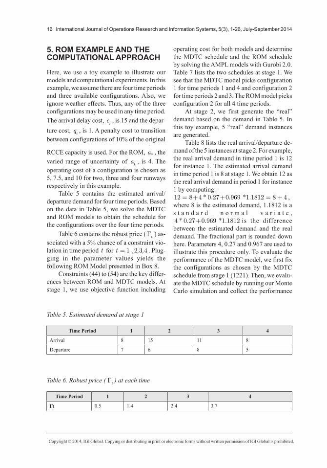
Table 5 contains the estimated arrival/ departure demand for four time periods. Based on the data in Table 5, we solve the MDTC and ROM models to obtain the schedule for the configurations over the four time periods.

Table 6 contains the robust price (Γt) as-

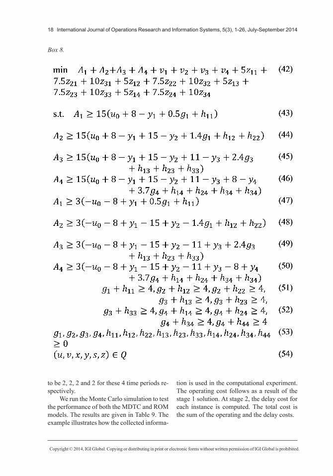
sociated with a 5% chance of a constraint vio-lation in time period t for t = 1 2 3 4�, ,� ,� . Plug-ging in the parameter values yields the following ROM Model presented in Box 8.

Constraints (44) to (54) are the key differ-ences between ROM and MDTC models. At stage 1, we use objective function including

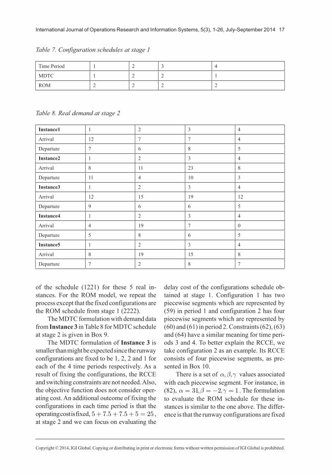
operating cost for both models and determine the MDTC schedule and the ROM schedule by solving the AMPL models with Gurobi 2.0. Table 7 lists the two schedules at stage 1. We see that the MDTC model picks configuration 1 for time periods 1 and 4 and configuration 2 for time periods 2 and 3. The ROM model picks configuration 2 for all 4 time periods.

At stage 2, we first generate the “real” demand based on the demand in Table 5. In this toy example, 5 “real” demand instances are generated.

Table 8 lists the real arrival/departure de-mand of the 5 instances at stage 2. For example, the real arrival demand in time period 1 is 12 for instance 1. The estimated arrival demand in time period 1 is 8 at stage 1. We obtain 12 as the real arrival demand in period 1 for instance 1 by computing:12 8 4 0 27 0 969 1 1812 8 4= + + = +� � * . � � . �* . ,where 8 is the estimated demand, 1.1812 is a s t a n d a r d n o r m a l v a r i a t e , 4 0 27 0 969 1 1812* . . * .+ is the difference between the estimated demand and the real demand. The fractional part is rounded down here. Parameters 4, 0.27 and 0.967 are used to illustrate this procedure only. To evaluate the performance of the MDTC model, we first fix the configurations as chosen by the MDTC schedule from stage 1 (1221). Then, we evalu-ate the MDTC schedule by running our Monte Carlo simulation and collect the performance

Table 5. Estimated demand at stage 1

Time Period 1 2 3 4

Arrival 8 15 11 8

Departure 7 6 8 5

Table 6. Robust price ( Γt) at each time

Time Period 1 2 3 4

𝚪t 0.5 1.4 2.4 3.7



of the schedule (1221) for these 5 real in-stances. For the ROM model, we repeat the process except that the fixed configurations are the ROM schedule from stage 1 (2222).

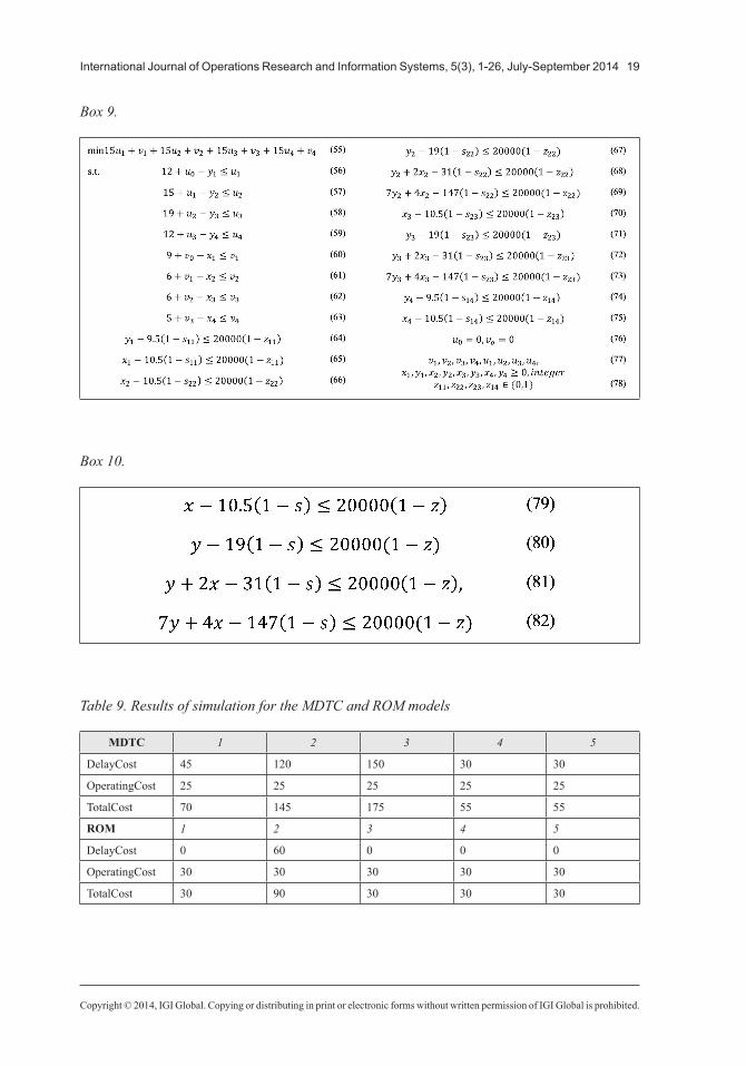
The MDTC formulation with demand data from Instance 3 in Table 8 for MDTC schedule at stage 2 is given in Box 9.

The MDTC formulation of Instance 3 is smaller than might be expected since the runway configurations are fixed to be 1, 2, 2 and 1 for each of the 4 time periods respectively. As a result of fixing the configurations, the RCCE and switching constraints are not needed. Also, the objective function does not consider oper-ating cost. An additional outcome of fixing the configurations in each time period is that the operating cost is fixed, 5 7 5 7 5 5 25+ + + =. . , at stage 2 and we can focus on evaluating the

delay cost of the configurations schedule ob-tained at stage 1. Configuration 1 has two piecewise segments which are represented by (59) in period 1 and configuration 2 has four piecewise segments which are represented by (60) and (61) in period 2. Constraints (62), (63) and (64) have a similar meaning for time peri-ods 3 and 4. To better explain the RCCE, we take configuration 2 as an example. Its RCCE consists of four piecewise segments, as pre-sented in Box 10.

There is a set of α β γ, , values associated with each piecewise segment. For instance, in (82), α β γ= = − =31 2 1, , . The formulation to evaluate the ROM schedule for these in-stances is similar to the one above. The differ-ence is that the runway configurations are fixed

Table 7. Configuration schedules at stage 1

Time Period 1 2 3 4

MDTC 1 2 2 1

ROM 2 2 2 2

Table 8. Real demand at stage 2

Instance1 1 2 3 4

Arrival 12 7 7 4

Departure 7 6 8 5

Instance2 1 2 3 4

Arrival 8 11 23 8

Departure 11 4 10 3

Instance3 1 2 3 4

Arrival 12 15 19 12

Departure 9 6 6 5

Instance4 1 2 3 4

Arrival 4 19 7 0

Departure 5 8 6 5

Instance5 1 2 3 4

Arrival 8 19 15 8

Departure 7 2 8 7



to be 2, 2, 2 and 2 for these 4 time periods re-spectively.

We run the Monte Carlo simulation to test the performance of both the MDTC and ROM models. The results are given in Table 9. The example illustrates how the collected informa-

tion is used in the computational experiment. The operating cost follows as a result of the stage 1 solution. At stage 2, the delay cost for each instance is computed. The total cost is the sum of the operating and the delay costs.

Box 8.



Table 9. Results of simulation for the MDTC and ROM models

MDTC 1 2 3 4 5

DelayCost 45 120 150 30 30

OperatingCost 25 25 25 25 25

TotalCost 70 145 175 55 55

ROM 1 2 3 4 5

DelayCost 0 60 0 0 0

OperatingCost 30 30 30 30 30

TotalCost 30 90 30 30 30

Box 9.

Box 10.



6. RESULTS AND COMPARISONS

In this section we return to the 20 time pe-riod data generated from the JFK dataset and compare and contrast the solutions found by the MTDC and ROM models. For the ROM model, we provide computational experience with a branch and bound stopping condition, the gap between the bound and the current best feasible solution.

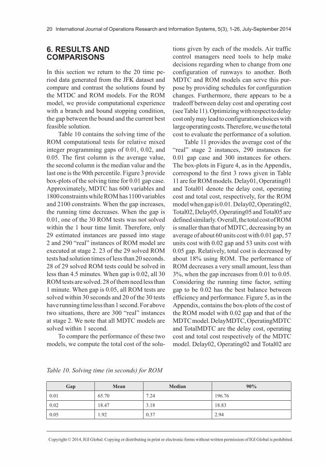
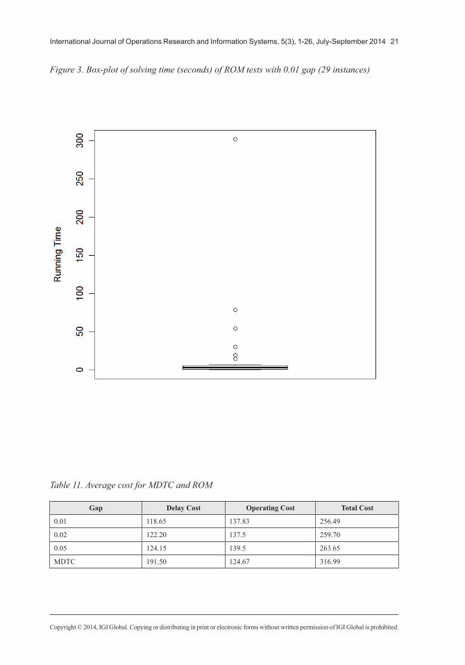
Table 10 contains the solving time of the ROM computational tests for relative mixed integer programming gaps of 0.01, 0.02, and 0.05. The first column is the average value, the second column is the median value and the last one is the 90th percentile. Figure 3 provide box-plots of the solving time for 0.01 gap case. Approximately, MDTC has 600 variables and 1800 constraints while ROM has 1100 variables and 2100 constraints. When the gap increases, the running time decreases. When the gap is 0.01, one of the 30 ROM tests was not solved within the 1 hour time limit. Therefore, only 29 estimated instances are passed into stage 2 and 290 “real” instances of ROM model are executed at stage 2. 23 of the 29 solved ROM tests had solution times of less than 20 seconds. 28 of 29 solved ROM tests could be solved in less than 4.5 minutes. When gap is 0.02, all 30 ROM tests are solved. 28 of them need less than 1 minute. When gap is 0.05, all ROM tests are solved within 30 seconds and 20 of the 30 tests have running time less than 1 second. For above two situations, there are 300 “real” instances at stage 2. We note that all MDTC models are solved within 1 second.

To compare the performance of these two models, we compute the total cost of the solu-

tions given by each of the models. Air traffic control managers need tools to help make decisions regarding when to change from one configuration of runways to another. Both MDTC and ROM models can serve this pur-pose by providing schedules for configuration changes. Furthermore, there appears to be a tradeoff between delay cost and operating cost (see Table 11). Optimizing with respect to delay cost only may lead to configuration choices with large operating costs. Therefore, we use the total cost to evaluate the performance of a solution.

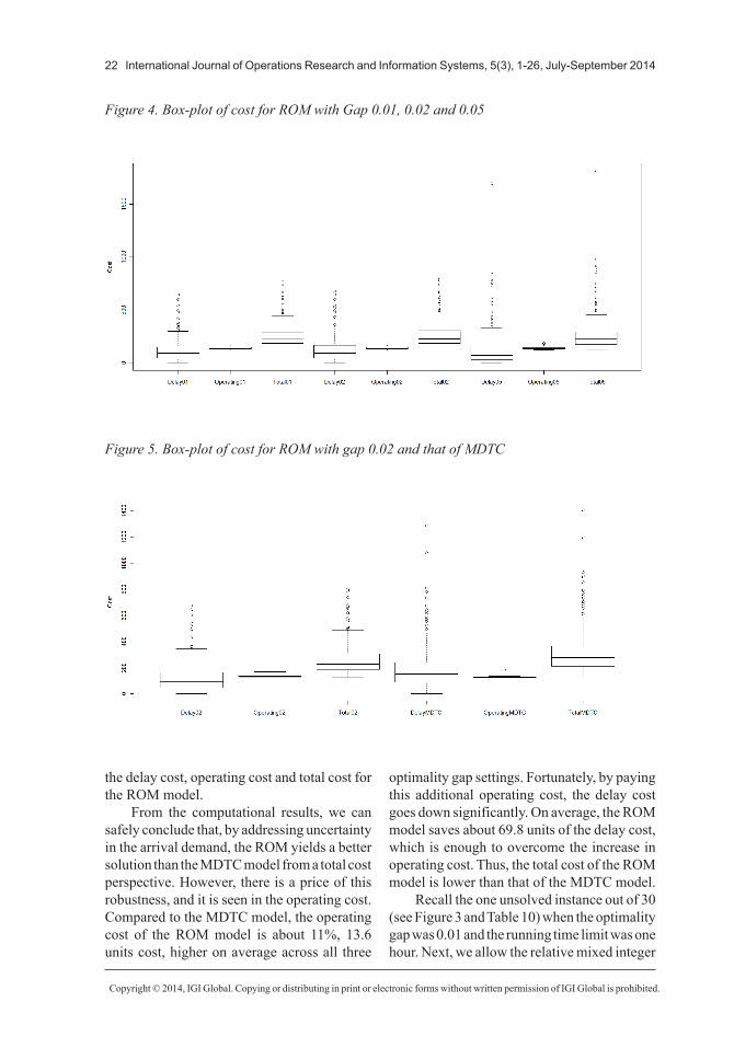
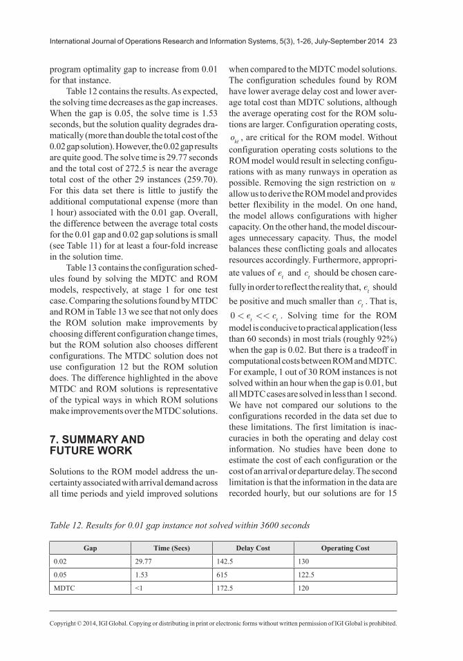
Table 11 provides the average cost of the “real” stage 2 instances, 290 instances for 0.01 gap case and 300 instances for others. The box-plots in Figure 4, as in the Appendix, correspond to the first 3 rows given in Table 11 are for ROM models. Delay01, Operating01 and Total01 denote the delay cost, operating cost and total cost, respectively, for the ROM model when gap is 0.01. Delay02, Operating02, Total02, Delay05, Operating05 and Total05 are defined similarly. Overall, the total cost of ROM is smaller than that of MDTC, decreasing by an average of about 60 units cost with 0.01 gap, 57 units cost with 0.02 gap and 53 units cost with 0.05 gap. Relatively, total cost is decreased by about 18% using ROM. The performance of ROM decreases a very small amount, less than 3%, when the gap increases from 0.01 to 0.05. Considering the running time factor, setting gap to be 0.02 has the best balance between efficiency and performance. Figure 5, as in the Appendix, contains the box-plots of the cost of the ROM model with 0.02 gap and that of the MDTC model. DelayMDTC, OperatingMDTC and TotalMDTC are the delay cost, operating cost and total cost respectively of the MDTC model. Delay02, Operating02 and Total02 are

Table 10. Solving time (in seconds) for ROM

Gap Mean Median 90%

0.01 65.70 7.24 196.76

0.02 18.47 3.18 18.83

0.05 1.92 0.37 2.94



Figure 3. Box-plot of solving time (seconds) of ROM tests with 0.01 gap (29 instances)

Table 11. Average cost for MDTC and ROM

Gap Delay Cost Operating Cost Total Cost

0.01 118.65 137.83 256.49

0.02 122.20 137.5 259.70

0.05 124.15 139.5 263.65

MDTC 191.50 124.67 316.99



the delay cost, operating cost and total cost for the ROM model.

From the computational results, we can safely conclude that, by addressing uncertainty in the arrival demand, the ROM yields a better solution than the MDTC model from a total cost perspective. However, there is a price of this robustness, and it is seen in the operating cost. Compared to the MDTC model, the operating cost of the ROM model is about 11%, 13.6 units cost, higher on average across all three

optimality gap settings. Fortunately, by paying this additional operating cost, the delay cost goes down significantly. On average, the ROM model saves about 69.8 units of the delay cost, which is enough to overcome the increase in operating cost. Thus, the total cost of the ROM model is lower than that of the MDTC model.

Recall the one unsolved instance out of 30 (see Figure 3 and Table 10) when the optimality gap was 0.01 and the running time limit was one hour. Next, we allow the relative mixed integer

Figure 4. Box-plot of cost for ROM with Gap 0.01, 0.02 and 0.05

Figure 5. Box-plot of cost for ROM with gap 0.02 and that of MDTC



program optimality gap to increase from 0.01 for that instance.

Table 12 contains the results. As expected, the solving time decreases as the gap increases. When the gap is 0.05, the solve time is 1.53 seconds, but the solution quality degrades dra-matically (more than double the total cost of the 0.02 gap solution). However, the 0.02 gap results are quite good. The solve time is 29.77 seconds and the total cost of 272.5 is near the average total cost of the other 29 instances (259.70). For this data set there is little to justify the additional computational expense (more than 1 hour) associated with the 0.01 gap. Overall, the difference between the average total costs for the 0.01 gap and 0.02 gap solutions is small (see Table 11) for at least a four-fold increase in the solution time.

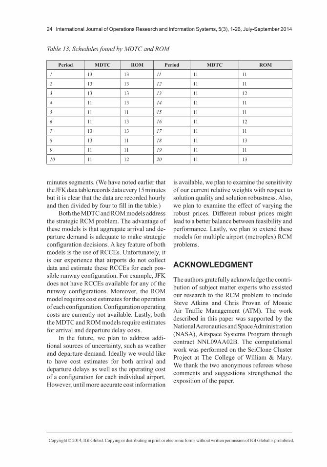
Table 13 contains the configuration sched-ules found by solving the MDTC and ROM models, respectively, at stage 1 for one test case. Comparing the solutions found by MTDC and ROM in Table 13 we see that not only does the ROM solution make improvements by choosing different configuration change times, but the ROM solution also chooses different configurations. The MTDC solution does not use configuration 12 but the ROM solution does. The difference highlighted in the above MTDC and ROM solutions is representative of the typical ways in which ROM solutions make improvements over the MTDC solutions.

7. SUMMARY AND FUTURE WORK

Solutions to the ROM model address the un-certainty associated with arrival demand across all time periods and yield improved solutions

when compared to the MDTC model solutions. The configuration schedules found by ROM have lower average delay cost and lower aver-age total cost than MDTC solutions, although the average operating cost for the ROM solu-tions are larger. Configuration operating costs, okt

, are critical for the ROM model. Without configuration operating costs solutions to the ROM model would result in selecting configu-rations with as many runways in operation as possible. Removing the sign restriction on u allow us to derive the ROM model and provides better flexibility in the model. On one hand, the model allows configurations with higher capacity. On the other hand, the model discour-ages unnecessary capacity. Thus, the model balances these conflicting goals and allocates resources accordingly. Furthermore, appropri-ate values of e

t and c

t should be chosen care-

fully in order to reflect the reality that, et should

be positive and much smaller than ct. That is,

0 < <<e ct t

. Solving time for the ROM model is conducive to practical application (less than 60 seconds) in most trials (roughly 92%) when the gap is 0.02. But there is a tradeoff in computational costs between ROM and MDTC. For example, 1 out of 30 ROM instances is not solved within an hour when the gap is 0.01, but all MDTC cases are solved in less than 1 second. We have not compared our solutions to the configurations recorded in the data set due to these limitations. The first limitation is inac-curacies in both the operating and delay cost information. No studies have been done to estimate the cost of each configuration or the cost of an arrival or departure delay. The second limitation is that the information in the data are recorded hourly, but our solutions are for 15

Table 12. Results for 0.01 gap instance not solved within 3600 seconds

Gap Time (Secs) Delay Cost Operating Cost

0.02 29.77 142.5 130

0.05 1.53 615 122.5

MDTC <1 172.5 120



minutes segments. (We have noted earlier that the JFK data table records data every 15 minutes but it is clear that the data are recorded hourly and then divided by four to fill in the table.)

Both the MDTC and ROM models address the strategic RCM problem. The advantage of these models is that aggregate arrival and de-parture demand is adequate to make strategic configuration decisions. A key feature of both models is the use of RCCEs. Unfortunately, it is our experience that airports do not collect data and estimate these RCCEs for each pos-sible runway configuration. For example, JFK does not have RCCEs available for any of the runway configurations. Moreover, the ROM model requires cost estimates for the operation of each configuration. Configuration operating costs are currently not available. Lastly, both the MDTC and ROM models require estimates for arrival and departure delay costs.

In the future, we plan to address addi-tional sources of uncertainty, such as weather and departure demand. Ideally we would like to have cost estimates for both arrival and departure delays as well as the operating cost of a configuration for each individual airport. However, until more accurate cost information

is available, we plan to examine the sensitivity of our current relative weights with respect to solution quality and solution robustness. Also, we plan to examine the effect of varying the robust prices. Different robust prices might lead to a better balance between feasibility and performance. Lastly, we plan to extend these models for multiple airport (metroplex) RCM problems.

ACKNOWLEDGMENT

The authors gratefully acknowledge the contri-bution of subject matter experts who assisted our research to the RCM problem to include Steve Atkins and Chris Provan of Mosaic Air Traffic Management (ATM). The work described in this paper was supported by the National Aeronautics and Space Administration (NASA), Airspace Systems Program through contract NNL09AA02B. The computational work was performed on the SciClone Cluster Project at The College of William & Mary. We thank the two anonymous referees whose comments and suggestions strengthened the exposition of the paper.

Table 13. Schedules found by MDTC and ROM

Period MDTC ROM Period MDTC ROM

1 13 13 11 11 11

2 13 13 12 11 11

3 13 13 13 11 12

4 11 13 14 11 11

5 11 11 15 11 11

6 11 13 16 11 12

7 13 13 17 11 11

8 13 11 18 11 13

9 11 11 19 11 11

10 11 12 20 11 13



REFERENCES

Atkin, J. A. D., Burke, E. K., Greenwood, J. S., & Reeson, D. (2008). On-line Decision Support for Take-off and Runway Scheduling with Uncertain Taxi Times at Heathrow Airport. Journal of Scheduling, 11(5), 323–346. doi:10.1007/s10951-008-0065-9

Ben-Tal, A., & Nemirovski, A. (1998). Robust convex optimization. Mathematics of Operations Research, 23(4), 769–805. doi:10.1287/moor.23.4.769

Ben-Tal, A., & Nemirovski, A. (1999). Robust solutions to uncertain programs. Operations Re-search Letters, 25(1), 1–13. doi:10.1016/S0167-6377(99)00016-4

Ben-Tal, A., & Nemirovski, A. (2000). Robust solu-tions of linear programming problems contaminated with uncertain data. Mathematical Programming, 88(3), 411–424. doi:10.1007/PL00011380

Bertsimas, D., Frankovich, M., & Odoni, A. (2009). Optimal Selection of Airport Runway Configura-tions. INFORMS Annual Meeting, San Diego, CA, October 11-14.

Bertsimas, D., & Sim, M. (2004). The price of robustness. Operations Research, 52(1), 35–52. doi:10.1287/opre.1030.0065

Bertsimas, D., & Thiele, A. (2006). A Robust Optimization Approach to Inventory Theory. Op-erations Research, 54(1), 150–168. doi:10.1287/opre.1050.0238

Das, N. (2009). The airport gate assignment problem with some practical constraints. International. Jour-nal of Applied Management Science, 1(3), 315–323.

de Neufville, R., & Odoni, A. (2003). Airport systems: Planning, design, and management. New York: McGraw-Hill.

El Ghaoui, L., & Lebret, H.El-Ghaoui. (1997). Ro-bust solutions to least-square problems to uncertain data matrices. SIAM Journal on Matrix Analysis and Applications, 18(4), 1035–1064. doi:10.1137/S0895479896298130

El-Ghaoui, L., Oustry, F., & Lebret, H. (1998). Robust solutions to uncertain semidefinite programs. SIAM Journal on Optimization, 9(1), 33–52. doi:10.1137/S1052623496305717

Federal Aviation Administration and MITRE Cor-poration. May 2007. Capacity Needs in the National Airspace System 2007-2025. http://www.faa.gov/airports/resources/publications/reports/media/fact_2.pdf. (7/23/2012)

Provan, C., & Atkins, S. (2010). Optimization Models for Strategic Runway Configuration Management Under Weather Uncertainty, Proceedings of the 10th AIAA Aviation Technology, Integration, & Operations (ATIO) Conference, Fort Worth, TX.

Soyster, A. L. (1973). Convex programming with set-inclusive constraints and applications to inexact linear programming. Operations Research, 21(5), 1154–1157. doi:10.1287/opre.21.5.1154

Technology Pathways. (2005). Assessing the Inte-grated Plan for a Next Generation Air Transportation System. National Academies Press.

The Sciclone Cluster Project, College of William and Mary, http://www.hpc.wm.edu/SciClone/index.html. (7/23/2012)

Thorne, J. A., & Kincaid, R. (2012). Tabu Search for Tactical Runway Configuration Management, to appear in Proceedings of the 12th AIAA Avia-tion Technology, Integration, & Operations (ATIO) Conference.

Tsao, H. S. J., & Pratama, A. (2011). A maximum-entropy approach to minimizing resource contention in aircraft routing for optimisation of airport surface operations. International Journal of Information and Decision Sciences, 3(4), 372–391. doi:10.1504/IJIDS.2011.043028

Weld, C., Duarte, M., & Kincaid, R. (2010). A Runway Configuration Management Model with Marginally Decreasing Transition Capacities, Ad-vances in Operations Research, Volume 2010, Article ID 436765, 21 pages.

Zhang, R., & Kincaid, R. (2011). Robust Optimi-zation for Runway Configuration Management, Proceedings of the 11th AIAA Aviation Technology, Integration, & Operations (ATIO) Conference, AIAA 2011-6922.

http://dx.doi.org/10.1007/s10951-008-0065-9

http://dx.doi.org/10.1287/moor.23.4.769

http://dx.doi.org/10.1016/S0167-6377(99)00016-4

http://dx.doi.org/10.1016/S0167-6377(99)00016-4

http://dx.doi.org/10.1007/PL00011380

http://dx.doi.org/10.1287/opre.1030.0065



http://dx.doi.org/10.1137/S0895479896298130

http://dx.doi.org/10.1137/S0895479896298130

http://dx.doi.org/10.1137/S1052623496305717

http://dx.doi.org/10.1137/S1052623496305717

http://www.faa.gov/airports/resources/publications/reports/media/fact_2.pdf



http://dx.doi.org/10.1287/opre.21.5.1154

http://www.hpc.wm.edu/SciClone/index.html

http://www.hpc.wm.edu/SciClone/index.html

http://dx.doi.org/10.1504/IJIDS.2011.043028

http://dx.doi.org/10.1504/IJIDS.2011.043028



Rui Zhang is a PhD student in Operations Management and Management Science at the Robert H Smith school of Business, University of Maryland, Maryland, USA. He received an M.S. degree in Computational Operations Research from the College of William and Mary. His research interests include integer programming, algorithm design and applied optimization in social networks. He presented his research at several international conferences, INFORMS computing society conference (ICS) and modeling and optimization: theory and applications (MOPTA). His article appeared in Naval Research Logistics (NRL).

Rex Kincaid (*) is a Professor in the Department of Mathematics, College of William and Mary, Virginia, USA. His M.S degree in Applied Mathematics and his Ph.D. in Operations Research are from Purdue University. His research interests include discrete optimization, complex systems, metaheuristics and network location theory. His peer reviewed research includes more than 40 undergraduate and masters degree students as co-authors. For the last 25 years he has worked on NASA funded research projects. In 2000 he received NASA’s group achievement award for his work on metaheuristics for active structural acoustic control.

Robust Optimization Model for Runway Configurations...

Documents

Transcript of Robust Optimization Model for Runway Configurations...