Robust Neural Network Regression for Offline and Online Learning

Thomas Briegel* Siemens AG, Corporate Technology

D-81730 Munich, Germany thomas.briegel@mchp.siemens.de

Volker Tresp Siemens AG, Corporate Technology

D-81730 Munich, Germany volker.tresp@mchp.siemens.de

Abstract

We replace the commonly used Gaussian noise model in nonlinear regression by a more flexible noise model based on the Student-t­distribution. The degrees of freedom of the t-distribution can be chosen such that as special cases either the Gaussian distribution or the Cauchy distribution are realized. The latter is commonly used in robust regres­sion. Since the t-distribution can be interpreted as being an infinite mix­ture of Gaussians, parameters and hyperparameters such as the degrees of freedom of the t-distribution can be learned from the data based on an EM-learning algorithm. We show that modeling using the t-distribution leads to improved predictors on real world data sets. In particular, if outliers are present, the t-distribution is superior to the Gaussian noise model. In effect, by adapting the degrees of freedom, the system can "learn" to distinguish between outliers and non-outliers. Especially for online learning tasks, one is interested in avoiding inappropriate weight changes due to measurement outliers to maintain stable online learn­ing capability. We show experimentally that using the t -distribution as a noise model leads to stable online learning algorithms and outperforms state-of-the art online learning methods like the extended Kalman filter algorithm.

1 INTRODUCTION

A commonly used assumption in nonlinear regression is that targets are disturbed by inde­pendent additive Gaussian noise. Although one can derive the Gaussian noise assumption based on a maximum entropy approach, the main reason for this assumption is practica­bility: under the Gaussian noise assumption the maximum likelihood parameter estimate can simply be found by minimization of the squared error. Despite its common use it is far from clear that the Gaussian noise assumption is a good choice for many practical prob­lems. A reasonable approach therefore would be a noise distribution which contains the Gaussian as a special case but which has a tunable parameter that allows for more flexible distributions. In this paper we use the Student-t-distribution as a noise model which con­tains two free parameters - the degrees of freedom 1/ and a width parameter (72. A nice feature of the t-distribution is that if the degrees of freedom 1/ approach infinity, we recover the Gaussian noise model. If 1/ < 00 we obtain distributions which are more heavy-tailed than the Gaussian distribution including the Cauchy noise model with 1/ = 1. The latter

*Now with McKinsey & Company, Inc.

408 T. Briegel and V. Tresp

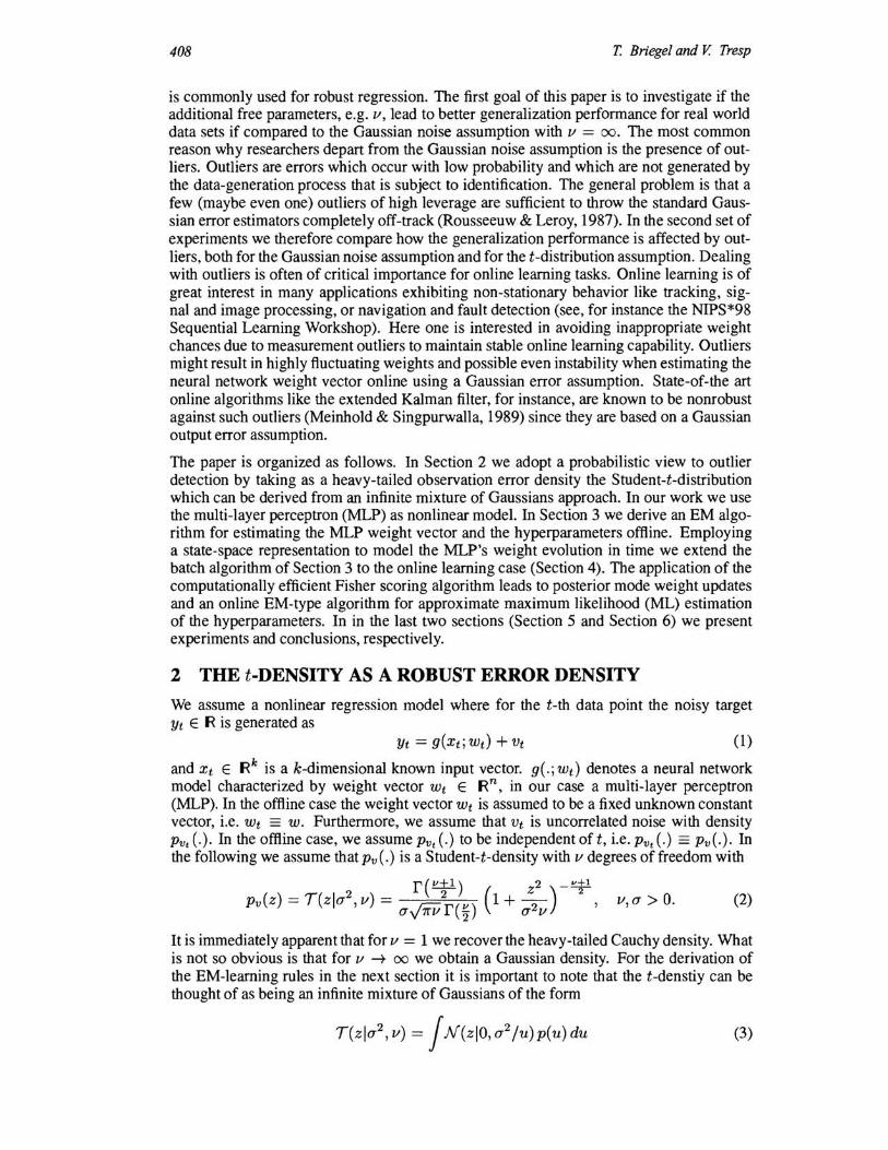
is commonly used for robust regression. The first goal of this paper is to investigate if the additional free parameters, e.g. v, lead to better generalization performance for real world data sets if compared to the Gaussian noise assumption with v = 00. The most common reason why researchers depart from the Gaussian noise assumption is the presence of out­liers. Outliers are errors which occur with low probability and which are not generated by the data-generation process that is subject to identification. The general problem is that a few (maybe even one) outliers of high leverage are sufficient to throw the standard Gaus­sian error estimators completely off-track (Rousseeuw & Leroy, 1987). In the second set of experiments we therefore compare how the generalization performance is affected by out­liers, both for the Gaussian noise assumption and for the t-distribution assumption. Dealing with outliers is often of critical importance for online learning tasks. Online learning is of great interest in many applications exhibiting non-stationary behavior like tracking, sig­nal and image processing, or navigation and fault detection (see, for instance the NIPS*98 Sequential Learning Workshop). Here one is interested in avoiding inappropriate weight chances due to measurement outliers to maintain stable online learning capability. Outliers might result in highly fluctuating weights and possible even instability when estimating the neural network weight vector online using a Gaussian error assumption. State-of-the art online algorithms like the extended Kalman filter, for instance, are known to be nonrobust against such outliers (Meinhold & Singpurwalla, 1989) since they are based on a Gaussian output error assumption.

The paper is organized as follows. In Section 2 we adopt a probabilistic view to outlier detection by taking as a heavy-tailed observation error density the Student-t-distribution which can be derived from an infinite mixture of Gaussians approach. In our work we use the multi-layer perceptron (MLP) as nonlinear model. In Section 3 we derive an EM algo­rithm for estimating the MLP weight vector and the hyperparameters offline. Employing a state-space representation to model the MLP's weight evolution in time we extend the batch algorithm of Section 3 to the online learning case (Section 4). The application of the computationally efficient Fisher scoring algorithm leads to posterior mode weight updates and an online EM-type algorithm for approximate maximum likelihood (ML) estimation of the hyperparameters. In in the last two sections (Section 5 and Section 6) we present experiments and conclusions, respectively.

2 THE t-DENSITY AS A ROBUST ERROR DENSITY

We assume a nonlinear regression model where for the t-th data point the noisy target Yt E R is generated as

(1)

and Xt E Rk is a k-dimensional known input vector. g(.;Wt) denotes a neural network model characterized by weight vector Wt E Rn , in our case a multi-layer perceptron (MLP). In the offline case the weight vector Wt is assumed to be a fixed unknown constant vector, i.e. Wt == w. Furthermore, we assume that Vt is uncorrelated noise with density Pv, (. ). In the offline case, we assume Pv, ( .) to be independent of t, i.e. Pv, (.) == Pv (.). In the following we assume that Pv (.) is a Student-t-density with v degrees of freedom with

r(!±l) z2-~ Pv(z)=T(zI0-2,v)= y'7W2qv)(1+-2-) , v,o->O. (2)

0- 1W 2" 0- V

It is immediately apparent that for v = 1 we recover the heavy-tailed Cauchy density. What is not so obvious is that for v -t 00 we obtain a Gaussian density. For the derivation of the EM-learning rules in the next section it is important to note that the t-denstiy can be thought of as being an infinite mixture of Gaussians of the form

(3)

Robust Neural Network Regression for Offline and Online Learning

3

2

-1 ._-._._ .. ... _ .. __ ..... . _ •• _"

2 ... ~,:,. - ..... ~ -...... -... -...... ... ;:~,'

-3 ,

-e -4 -2 ° z

, ". v-T5 . ,'; .. ,..................... ..~ ....

~ . ;,-_. __ .-.. ....... ::-: .... . - .-.-

2 4 "

Boeton Houaing ct.,_ with addtttve oult .... 1.2r-~-~--"-.--~----..."

1.1

liJO.9 0 .8

0 .7

0.5'----:---5~-7;;IO:-----:15~---;20~--::;!25 nu_ Of 0UIIIen ('K.]

409

Figure 1: Left: ¢(.)-functions for the Gaussian density (dashed) and t-densities with II = 1,4,15 degrees of freedom. Right: MSE on Boston Housing data test set for additive outliers. The dashed line shows results using a Gaussian error measure and the continuous line shows the results using the Student-t-distribution as error measure.

where T(zI0'2, II) is the Student-t-density with II degrees of freedom and width parameter 0'2, N(zIO, 0'2/U) is a Gaussian density with center 0 and variance 0'2/U and U '" X~/II where X~ is a Chi-square distribution with II degrees of freedom evaluated at U > O.

To compare different noise models it is useful to evaluate the "¢-function" defined as (Hu­ber,1964)

¢(z) = -ologpv(z)/oz (4) i.e. the negative score-function of the noise density. In the case of i.i.d. samples the ¢­function reflects the influence of a single measurement on the resulting estimator. Assum­ing Gaussian measurement errors Pv(z) = N(zIO,0'2) we derive ¢(z) = z/0'2 which means that for Izl -+ 00 a single outlier z can have an infinite leverage on the estimator. In contrast, for constructing robust estimators West (1981) states that large outliers should not have any influence on the estimator, i.e. ¢(z) -+ 0 for Izl -+ 00. Figure 1 (left) shows ¢(z) for different II for the Student-t-distribution. It can be seen that the degrees of freedom II determine how much weight outliers obtain in influencing the regression. In particular, for finite II, the influence of outliers with Izl -+ 00 approaches zero.

3 ROBUST OFFLINE REGRESSION

As stated in Equation (3), the t-density can be thought of as being generated as an infinite mixture of Gaussians. Maximum likelihood adaptation of parameters and hyperparameters can therefore be performed using an EM algorithm (Lange et al., 1989). For the t-th sample, a complete data point would consist of the triple (Xt, Yt, Ut) of which only the first two are known and Ut is missing.

In the E-step we estimate for every data point indexed by t

(5)

where at = E[ut IYt, Xt] is the expected value of the unknown Ut given the available data (Xt,Yt) andwhere«5t = (Yt - g(Xti W0 1d »)2 /0'2,old.

In the M-step the weights wand the hyperparameters 0'2 and II are optimized using

T

argm~n{LOt(Yt - g(Xt iW»)2} (6) t=l

410 T. Briegel and V. Tresp

T

~ L at [(Yt - g(Xt; wnew )) 2] (7) t=l

{ Tv v v argm:x T log 2" - Tlog{f( 2")}

T T

+( ~ - 1) L (3t - ~ L at} t=l t=l

(8)

where

(9)

with the Digamma function DG(z) = 8f(z)/8z. Note that the M-step for v is a one­dimensional nonlinear optimization problem. Also note that the M-steps for the weights in the MLP reduce to a weighted least squares regression problem in which outliers tend to be weighted down. The exception of course is the Gaussian case with v ~ 00 in which all terms obtain equal weight.

4 ROBUST ONLINE REGRESSION

For robust online regression, we assume that the model Equation (1) is still valid but that w can change over time, i.e. w = Wt. In particular we assume that Wt follows a first order random walk with normally distributed increments, i.e.

(10)

and where Wo is normally distributed with center ao and covariance Qo. Clearly, due to the nonlinear nature of 9 and due to the fact that the noise process is non-Gaussian, a fully Bayesian online algorithm - which for the linear case with Gaussian noise can be realized using the Kalman filter - is clearly infeasible.

On the other hand, if we consider data 'D = {Xt, yt}f=l' the negative log-posterior -logp(WTI'D) of the parameter sequence WT = (wJ, ... , w~) T is up to a normaliz­ing constant

-logp(WTI'D) ex:

and can be used as the appropriate cost function to derive the posterior mode estimate W¥AP for the weight sequence. The two differences to the presentation in the last section are that first, Wt is allowed to change over time and that second, penalty terms, stemming from the prior and the transition density, are included. The penalty terms are penalizing roughness of the weight sequence leading to smooth weight estimates.

A suitable way to determine a stationary point of -logp(WTI'D), the posterior mode es­timate of WT , is to apply Fisher scoring. With the current estimate WT1d we get a better estimate wTew = wTld +171' for the unknown weight sequence WT where 'Y is the solution of

(12)

with the negative score function S(WT) = -8logp(WT1'D)/8WT and the expected infor­mation matrix S(WT) = E[82 10gp(WTI'D)/8WT8WT ]. By applying the ideas given in Fahrmeir & Kaufmann (1991) to robust neural network regression it turns out that solving (12), i.e. to compute the inverse of the expected information matrix, can be performed by

Robust Neural Network Regression/or Offline and Online Learning 411

Cholesky decomposition in one forward and backward pass through the set of data 'D. Note that the expected information matrix is a positive definite block-tridiagonal matrix. The forward-backward steps have to be iterated to obtain the posterior mode estimate W.pAP

for WT.

For online posterior mode smoothing, it is of interest to smooth backwards after each filter step t. If Fisher scoring steps are applied sequentially for t = 1,2, ... , then the posterior mode smoother at time-step t - 1, wl~~~P = (W~t-l"'" wi-I lt-l) T together with the step-one predictor Wtlt-l = Wt-I lt-l is a reasonable starting value for obtaining the pos­terior mode smoother WtMAP at time t. One can reduce the computational load by limiting the backward pass to a sliding time window, e.g. the last Tt time steps, which is reasonable in non-stationary environments for online purposes. Furthermore, if we use the underly­ing assumption that in most cases a new measurement Yt should not change estimates too drastically then a single Fisher scoring step often suffices to obtain the new posterior mode estimate at time t. The resulting single Fisher scoring step algorithm with lookback param­eter Tt has in fact just one additional line of code involving simple matrix manipulations compared to online Kalman smoothing and is given here in pseudo-code. Details about the algorithm and a full description can be found in Briegel & Tresp (1999).

Online single Fisher scoring step algorithm (pseudo-code)

for t = 1,2, ... repeat the following four steps:

• Evaluate the step-one predictor Wt lt-l.

• Perform the forward recursions for s = t - Tt, ... , t.

• New data point (Xt, yd arrives: evaluate the corrector step Wtlt.

• Perform the backward smoothing recursions ws-Ilt for s = t, ... , t - Tt.

For the adaptation of the parameters in the t-distribution, we apply results from Fahrmeir & Kunstler (1999) to our nonlinear assumptions and use an online EM-type algorithm for approximate maximum likelihood estimation of the h yperparameters lit and (7F. We assume the scale factors (7F and the degrees of freedom lit being fixed quantities in a certain time window of length ft, e.g. (7F = (72, lit = 11, t E {t - ft, t}. For deriving online EM update equations we treat the weight sequence Wt together with the mixing variables Ut as missing. By linear Taylor series expansion of g(.; w s ) about the Fisher scoring solutions Wslt and by approximating posterior expectations E[ws I'D] with posterior modes Wslt, S E {t - ft, t} and posterior covariances cov[ws I'D] with curvatures :Eslt = E[( Ws - Wslt) (ws - Wslt) T I'D] in the E-step, a somewhat lengthy derivation results in approximate maximum likelihood update rules for (72 and 11 similar to those given in Section 3. Details about the online EM-type algorithm can be found in Briegel & Tresp (1999).

5 EXPERIMENTS 1. Experiment: Real World Data Sets. In the first experiment we tested if the Student­t-distribution is a useful error measure for real-world data sets. In training, the Student­t-distribution was used and both, the degrees of freedom 11 and the width parameter (72

were adapted using the EM update rules from Section 3. Each experiment was repeated 50 times with different divisions into training and test data. As a comparison we trained the neural networks to minimize the squared error cost function (including an optimized weight decay term). On the test data set we evaluated the performance using a squared error cost function. Table 1 provides some experimental parameters and gives the test set performance based on the 50 repetitions of the experiments. The additional explained variance is defined as [in percent] 100 x (1 - MSPE, IMSPEN) where MSPE, is the mean squared prediction error using the t-distribution and MSPEN is the mean squared prediction error using the Gaussian error measure. Furthermore we supply the standard

412 T. Briegel and V. Tresp

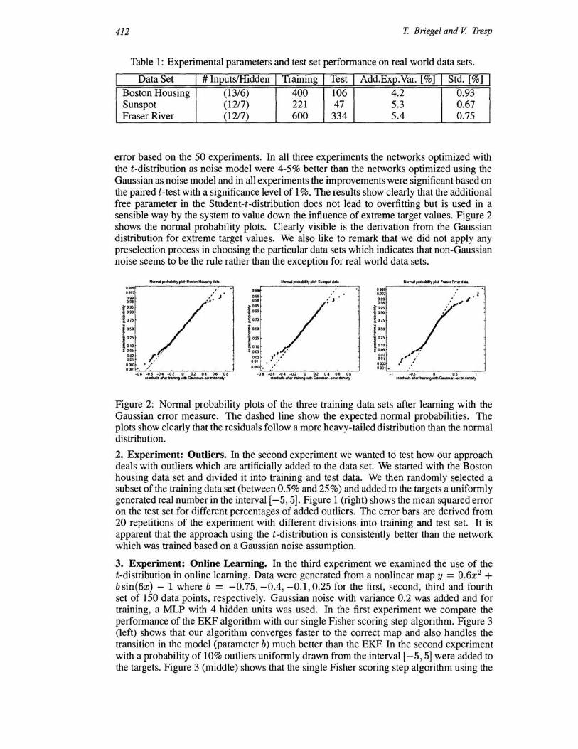
Table I: Experimental parameters and test set performance on real world data sets.

Data Set I # Inputs/Hidden I Training I Test I Add.Exp.Var. [%] I Std. [%] I Boston Housing (13/6) 400 106 4.2 0.93 Sunspot (1217) 221 47 5.3 0.67 Fraser River (1217) 600 334 5.4 0.75

error based on the 50 experiments. In all three experiments the networks optimized with the t-distribution as noise model were 4-5% better than the networks optimized using the Gaussian as noise model and in all experiments the improvements were significant based on the paired t-test with a significance level of 1 %. The results show clearly that the additional free parameter in the Student-t-distribution does not lead to overfitting but is used in a sensible way by the system to value down the influence of extreme target values. Figure 2 shows the normal probability plots. Clearly visible is the derivation from the Gaussian distribution for extreme target values. We also like to remark that we did not apply any preselection process in choosing the particular data sets which indicates that non-Gaussian noise seems to be the rule rather than the exception for real world data sets.

:: 0.99 0."

~095 1090

1075

i oso

i0 25

1010 ; 005

002 00\ 0003

000' ''-._0-, ~--="-<>5o-----O-0 - ---,07' - -',---' ,e~"""MWlgWllllh~ .. -8fTttdenllly

Figure 2: Normal probability plots of the three training data sets after learning with the Gaussian error measure. The dashed line show the expected normal probabilities. The plots show clearly that the residuals follow a more heavy-tailed distribution than the normal distribution.

2. Experiment: Outliers. In the second experiment we wanted to test how our approach deals with outliers which are artificially added to the data set. We started with the Boston housing data set and divided it into training and test data. We then randomly selected a subset of the training data set (between 0.5% and 25%) and added to the targets a uniformly generated real number in the interval [-5,5]. Figure I (right) shows the mean squared error on the test set for different percentages of added outliers. The error bars are derived from 20 repetitions of the experiment with different divisions into training and test set. It is apparent that the approach using the t-distribution is consistently better than the network which was trained based on a Gaussian noise assumption.

3. Experiment: Online Learning. In the third experiment we examined the use of the t-distribution in online learning. Data were generated from a nonlinear map y = 0.6X2 + bsin(6x) - 1 where b = -0.75, -0.4, -0.1,0.25 for the first, second, third and fourth set of 150 data points, respectively. Gaussian noise with variance 0.2 was added and for training, a MLP with 4 hidden units was used. In the first experiment we compare the performance of the EKF algorithm with our single Fisher scoring step algorithm. Figure 3 (left) shows that our algorithm converges faster to the correct map and also handles the transition in the model (parameter b) much better than the EKE In the second experiment with a probability of 10% outliers uniformly drawn from the interval [-5,5] were added to the targets. Figure 3 (middle) shows that the single Fisher scoring step algorithm using the

Robust Neural Network Regression/or Offline and Online Learning 413

t-distribution is consistently better than the same algorithm using a Gaussian noise model and the EKE The two plots on the right in Figure 3 compare the nonlinear maps learned after 150 and 600 time steps, respectively.

w ~ . !

IO~O~-C'00::---=200~-=311l;--::::""'--5;:;;1Il-----:!1Dl r",.

1~'

10 0

'.

100 2CIO 300 400 5CXl all r",.

0.5

Figure 3: Left & Middle: Online MSE over each of the 4 sets of training data. On the left we compare extended Kalman filtering (EKF) (dashed) with the single Fisher scoring step algorithm with Tt = 10 (GFS-lO) (continuous) for additive Gaussian noise. The second figure shows EKF (dashed-dotted), Fisher scoring with Gaussian error noise (GFS-1 0) (dashed) and t-distributed error noise (TFS-l 0) (continuous), respectively for data with additive outliers. Right: True map (continuous), EKF learned map (dashed-dotted) and TFS-I0 map (dashed) after T = 150 and T = 600 (data sets with additive outliers).

6 CONCLUSIONS

We have introduced the Student-t-distribution to replace the standard Gaussian noise as­sumption in nonlinear regression. Learning is based on an EM algorithm which estimates both the scaling parameters and the degrees of freedom of the t-distribution. Our results show that using the Student-t-distribution as noise model leads to 4-5% better test errors than using the Gaussian noise assumption on real world data set. This result seems to in­dicate that non-Gaussian noise is the rule rather than the exception and that extreme target values should in general be weighted down. Dealing with outliers is particularly important for online tasks in which outliers can lead to instability in the adaptation process. We in­troduced a new online learning algorithm using the t-distribution which leads to better and more stable results if compared to the extended Kalman filter.

References

Briegel, T. and Tresp, V. (1999) Dynamic Neural Regression Models, Discussion Paper, Seminar flir Statistik, Ludwig Maximilians Universitat Milnchen. de Freitas, N., Doucet, A. and Niranjan, M. (1998) Sequential Inference and Learning, NIPS*98 Workshop, Breckenridge, CO.

Fahrmeir, L. and Kaufmann, H. (1991) On Kalman Filtering, Posterior Mode Estimation and Fisher Scoring in Dynamic Exponential Family Regression, Metrika 38, pp. 37-60.

Fahrmeir, L. and Kilnstler, R. (1999) Penalized Likelihood smoothing in robust state space models, Metrika 49, pp. 173-191. Huber, p.r. (1964) Robust Estimation of Location Parameter, Annals of Mathematical Statistics 35, pp.73-101. Lange, K., Little, L., Taylor, J. (989) Robust Statistical Modeling Using the t-Distribution, JASA 84, pp. 881-8%.

Meinhold, R. and SingpurwaIla, N. (1989) Robustification of Kalman Filter Models, JASA 84, pp. 470-496. Rousseeuw, P. and Leroy, A. (1987) Robust Regression and Outlier Detection, John Wiley & Sons.

West, M. (1981) Robust Sequential Approximate Bayesian Estimation, JRSS B 43, pp. 157-166.