
Robust Machine Learning QSPR Models for Recognizing High ...
133
Robust Machine Learning QSPR Models for Recognizing High Performing MOFs for Pre-Combustion Carbon Capture and Using Molecular Simulation to Study Adsorption of Water and Gases in Novel MOFs Hana Dureckova Thesis submitted to the Faculty of Graduate and Postdoctoral Studies in partial fulfillment of the requirements for the degree of Master in Chemistry Department of Chemistry and Biomolecular Sciences Faculty of Science University of Ottawa © Hana Dureckova, Ottawa, Canada, 2018
Transcript of Robust Machine Learning QSPR Models for Recognizing High ...

Robust Machine Learning QSPR Models for Recognizing High
Performing MOFs for Pre-Combustion Carbon Capture
and Using Molecular Simulation to Study Adsorption of
Water and Gases in Novel MOFs
Hana Dureckova
Thesis submitted to the
Faculty of Graduate and Postdoctoral Studies
in partial fulfillment of the requirements for the degree of
Master in Chemistry
Department of Chemistry and Biomolecular Sciences
Faculty of Science
University of Ottawa
© Hana Dureckova, Ottawa, Canada, 2018
ii
Contents
Abstract ........................................................................................................................................... v
Table of Figures ............................................................................................................................ vii
List of Tables .................................................................................................................................. x
List of Acronyms ........................................................................................................................... xi
Acknowledgements ....................................................................................................................... xii
1 Introduction ............................................................................................................................. 1
1.1 Carbon Capture and Storage (CCS) ................................................................................. 1
1.1.1 Post-combustion Carbon Capture ................................................................................. 2
1.1.2 Pre-combustion Carbon Capture .................................................................................. 5
1.2 Metal-Organic Frameworks (MOFs) ............................................................................... 7
1.3 Evaluating MOFs for CCS Applications ........................................................................ 10
1.3.1 Working capacity ........................................................................................................ 10
1.3.2 Selectivity ................................................................................................................... 12
1.3.3 MOF Stability ............................................................................................................. 13
1.4 MOF Structural Characterization ................................................................................... 14
1.5 Molecular Simulation of MOFs ..................................................................................... 15
1.6 Computational Approaches in MOF Discovery ............................................................. 16
1.7 Thesis Goals and Outline ............................................................................................... 18
1.8 References ...................................................................................................................... 20
2 Methods ................................................................................................................................. 24
2.1 Periodic Density Functional Theory (DFT) ................................................................... 24
2.2 REPEAT Charge Calculation ......................................................................................... 26
2.3 Grand Canonical Monte Carlo Simulation (GCMC) ..................................................... 27
2.4 Automatic Binding Site Locator (ABSL)....................................................................... 29
2.5 Quantitative Structure-Property Relationship (QSPR) .................................................. 30
2.5.1 Descriptors and Target Properties .............................................................................. 31
2.5.2 QSPR Modeling Methods ........................................................................................... 33
2.5.3 Support Vector Machines ........................................................................................... 34
2.5.4 Training of SVR Model .............................................................................................. 40

iii
2.5.5 Validation of SVR Model ........................................................................................... 41
2.6 References ...................................................................................................................... 42
3 Robust Quantitative Structure-Property Relationship (QSPR) Models for Recognizing Metal
Organic Frameworks (MOFs) with High CO2 Working Capacity and CO2/H2 Selectivity for Pre-
combustion Carbon Capture ......................................................................................................... 44
3.1 Abstract .......................................................................................................................... 44
3.2 Introduction .................................................................................................................... 45
3.3 MOF Database and Computational Methods ................................................................. 48
3.3.1 Hypothetical MOF Database and GCMC Simulations............................................... 48
3.3.2 Atomic Property-Weighted Radial Distribution Functions as Descriptors for MOFs 51
3.3.3 Support Vector Regression Models ............................................................................ 52
3.4 Results and Discussion ................................................................................................... 54
3.4.1 Performance of the SVR Models ................................................................................ 54
3.4.2 Further Validation and Application of the SVR Models ............................................ 59
3.5 Summary and Conclusions ............................................................................................. 61
3.6 References ...................................................................................................................... 63
4 Modeling CO2 and H2O Adsorption in CALF-20, the “Magic MOF” .................................. 65
4.1 Abstract .......................................................................................................................... 65
4.2 Introduction .................................................................................................................... 66
4.3 Computational Details .................................................................................................... 69
4.4 Results ............................................................................................................................ 71
4.4.1 Determination of the Crystal Structure of CALF-20 .................................................. 71
4.4.2 CO2 and H2O Adsorption Properties of CALF-20 ..................................................... 75
4.4.3 CO2 and H2O Binding Site Analysis for CALF-20 .................................................... 83
4.5 Conclusions .................................................................................................................... 86
4.6 References ...................................................................................................................... 89
5 Modeling CH4 and N2 adsorption in the Ni-BPM MOF Containing Residual Solvent ........ 91
5.1 Abstract .......................................................................................................................... 91
5.2 Introduction .................................................................................................................... 92
5.3 Computational Details .................................................................................................... 95
5.4 Results ............................................................................................................................ 98

iv
5.4.1 Single Crystal X-Ray Diffraction (SCXRD) Data ..................................................... 98
5.4.2 Computational Results .............................................................................................. 100
5.5 Conclusions .................................................................................................................. 111
5.6 References .................................................................................................................... 113
6 Conclusion ........................................................................................................................... 114
6.1 Summary ...................................................................................................................... 114
6.2 Publications .................................................................................................................. 117
6.2.1 Thesis-Related Publications ..................................................................................... 117
6.2.2 Other Publications on Topics Not Related to Thesis Projects .................................. 117
6.3 Future Work ................................................................................................................. 117
6.3.1 Robust QSPR Models for Recognizing MOFs with High CO2 Working Capacity and
CO2/H2 Selectivitiy for Pre-combustion Carbon Capture ................................................... 117
6.3.2 Modeling CO2 and H2O Adsorption in CALF-20, the “Magic MOF” ..................... 119
6.3.3 Modeling CH4 and N2 Adsorption in the Ni-BPM MOF ......................................... 119
6.4 References .................................................................................................................... 120
7 Appendices .......................................................................................................................... 121

v
Abstract
Metal organic frameworks (MOFs) are a class of nanoporous materials composed
through self-assembly of inorganic and organic structural building units (SBUs). MOFs show
great promise for many applications due to their record-breaking internal surface areas and
tunable pore chemistry. This thesis work focuses on gas separation applications of MOFs in the
context of carbon capture and storage (CCS) technologies. CCS technologies are expected to
play a key role in the mitigation of anthropogenic CO2 emissions in the near future.
In the first part of the thesis, robust machine learning quantitative structure-property
relationship (QSPR) models are developed to predict CO2 working capacity and CO2/H2
selectivity for pre-combustion carbon capture using the most topologically diverse database of
hypothetical MOF structures constructed to date (358,400 MOFs, 1166 network topologies). The
support vector regression (SVR) models are developed on a training set of 35,840 MOFs (10% of
the database) and validated on the remaining 322,560 MOFs. The most accurate models for CO2
working capacities (R2 = 0.944) and CO2/H2 selectivities (R2 = 0.876) are built from a
combination of six geometric descriptors and three novel y-range normalized atomic-property-
weighted radial distribution function (AP-RDF) descriptors. 309 common MOFs are identified
between the grand canonical Monte Carlo (GCMC) calculated and SVR-predicted top-1000
high-performing MOFs ranked according to a normalized adsorbent performance score
(𝐴𝑃𝑆𝑛𝑜𝑟𝑚). This work shows that SVR models can indeed account for the topological diversity
exhibited by MOFs.
In the second project of this thesis, computational simulations are performed on a MOF,
CALF-20, to examine its chemical and physical properties which are linked to its exceptional
water-resisting ability. We predict the atomic positions in the crystal structure of the bulk phase

vi
of CALF-20, for which only a powder X-ray diffraction pattern is available, from a single crystal
X-ray diffraction pattern of a metastable phase of CALF-20. Using the predicted CALF-20
structure, we simulate adsorption isotherms of CO2 and N2 under dry and humid conditions
which are in excellent agreement with experiment. Snapshots of the CALF-20 undergoing water
sorption simulations reveal that water molecules in a given pore adsorb and desorb together due
to hydrogen bonding. Binding sites and binding energies of CO2 and water in CALF-20 show
that the preferential CO2 uptake at low relative humidities is driven by the stronger binding
energy of CO2 in the MOF, and the sharp increase in water uptake at higher relative humidities is
driven by the strong intermolecular interactions between water.
In the third project of this thesis, we use computational simulations to investigate the
effects of residual solvent on Ni-BPM’s CH4 and N2 adsorption properties. Single crystal X-ray
diffraction data shows that there are two sets of positions (Set 1 and 2) that can be occupied by
the 10 residual DMSO molecules in the Ni-BPM framework. GCMC simulations of CH4 and N2
uptake in Ni-BPM reveal that CH4 uptake is in closest agreement with experiment when the 10
DMSO’s are placed among the two sets of positions in equal ratio (Mixed Set). Severe under-
prediction and over-prediction of CH4 uptake are observed when the DMSO’s are placed in Set1
and Set 2 positions, respectively. Through binding site analysis, the CH4 binding sites within the
Ni-BPM framework are found to overlap with the Set 1 DMSO positions but not with the Set 2
DMSO positions which explains the deviations in CH4 uptake observed for these cases. Binding
energy calculations reveal that CH4 molecules are most stabilized when the DMSO’s are in the
Mixed Set of positions.

vii
Table of Figures
Figure 1.1: a) The components of MOF-5 showing the abstraction of the Zn4O(-CO2)6 SBU as
an octahedron, the ditopic terephthalate linker as a rod and their assembly into the pcu network
topology. b) MOF-5 shown through the {100} plane. .................................................................... 8
Figure 1.2: Examples of network topologies. ................................................................................ 8
Figure 1.3: Adsorption isotherm of CO2 in a MOF. The closed circle represents the uptake of
CO2 at the CO2 partial pressure relevant to pre-combustion carbon capture, while the open one
represents the uptake under desorption condition. Δ𝑞 represent the CO2 working capacity. ....... 11
Figure 2.1: The green line represents an overfitted model and the black line represents a
regularized model. While the green line best follows the training data, it is too data-dependent
thus it is likely to have a higher error rate on new unseen data compared to the black line. ........ 35
Figure 2.2: An example of a linearly separable two-class data with possible separating lines.
Lines in light blue are non-optimal lines for characterizing the two data classes while the line in
dark blue is an optimal line which SVM attempts to find.38 ......................................................... 37
Figure 2.3: An example of noisy data, where SVM finds an optimal hyperplane (blue line) by
maximizing margin (m) and allowing some points to be misclassified or to be in the margin.38 38
Figure 2.4: A representation of mapping descriptor vectors from an input space onto a feature
space where data is linearly separable. ......................................................................................... 39
Figure 3.1: Histograms of a) gravimetric surface area, b) largest accessible pore size, and
GCMC-calculated c) CO2 working capacity and d) CO2/H2 selectivity for the database of
358,400 hypothetical MOF structures. The dotted lines represent performance of experimentally
synthesized MOFs which have been studied for pre-combustion carbon capture, namely Ni-
4PyC, MgMOF-74 and CuBTTri. ................................................................................................. 51
Figure 3.2: A flowchart outlining the internal four-fold-out cross-validation procedure used to
train the SVR models of CO2 working capacity and CO2/H2 selectivity. ..................................... 54
Figure 3.3: Heatmaps of a),b) SVR-predicted CO2 working capacity plotted against GCMC-
calculated CO2 working capacity and c),d) SVR-predicted CO2/H2 selectivity plotted against
GCMC-calculated CO2/H2 selectivity for the 332,560 MOFs in the test set. The SVR models
shown in a) and c) were built using the unnormalized AP-RDF descriotors with six geometric
descriptors and the SVR models shown in b) and d) were built using the y-range normalized AP-
RDF descriptors with six geometric descriptors. The AP-RDFs were weighted by
electronegativity, hardness and van der Waals volume. R2 values shown indicate how well the
SVR predictions match GCMC calculations. The colours of the heatmaps correspond to number
of MOFs, where red is high and blue is low. ................................................................................ 56

viii
Figure 3.4: Heatmaps of a) GCMC-calculated and b) SVR-predicted CO2 working capacity
plotted against CO2/H2 selectivity for the test set containing 332,560 MOFs. The colours of the
heatmaps correspond to number of MOFs, where red is high and blue is low. ............................ 59
Figure 4.1: CO2 breakthrough experiments on CALF-20 at 0%, 20% and 40% relative humidity.
The ratio of CO2 concentrations at output and input (C/C0) for each run is plotted against time.
Adsorption kinetics are not affected by water. ............................................................................. 68
Figure 4.2: (a) PXRD of the experimental (Expt.) metastable phase and the predicted and
experimental bulk phases of CALF-20. (b) Structure for the predicted bulk phase in the b-c plane
and (c) a-c plane with atom labels corresponding to geometric parameters summarized in Table
2. Selected bond lengths are shown for the DFT optimized bulk phase and metastable phase (in
parenthesis) from SCXRD. ........................................................................................................... 74
Figure 4.3: a) Experimental and simulated single component sorption isotherms of the bulk
phase of CALF-20 for CO2 and N2 at 293 K. The simulated CO2 isotherm of the metastable
phase of CALF-20 is also shown. b) Simulated binary gas sorption isotherms for CO2 and N2
(20:80) at 293 K for the predicted bulk phase of CALF-20 are compared with experimental
binary gas sorption isotherms derived using IAST. ...................................................................... 76
Figure 4.4: a) Experimental (Expt.) water sorption isotherms for Zeolite 13X and CALF-20 at
293 K and b) Experimental (Expt.) and simulated (Sim.) water sorption isotherms of CALF-20 at
293 K. In both experimental and simulated results, adsorption and desorption data are shown. c)
Simulated gas sorption isotherms of CALF-20 for CO2, N2 and H2O at 293 K. The ratio of
CO2:N2 and was kept at 20:80 with a total pressure of 1 bar. The amount of H2O ranged from
0.002338 to 0.02338 bar which corresponds to 10-100 % relative humidity at 293 K. Pure water
adsorption isotherm at 293 K is also shown for comparison. ....................................................... 79
Figure 4.5: A snap shot from a 100% relative humidity simulation of CALF-20 showing all
pores are filled with water. The views are from the b-c, a-b and a-c planes of CALF-20. ......... 80
Figure 4.6: a) Plot of the number of water molecules adsorbed onto CALF-20 in equilibrium at
20% relative humidity as a function of GCMC steps. This GCMC simulation began on a
previously equilibrated system. Dotted lines represent 50 million and 94 million steps for which
snapshots are presented in b). The circles in b) show pores with notable changes in the number of
adsorbed water molecules. ............................................................................................................ 82
Figure 4.7: Isosurface plots of the probability distributions of CO2 in CALF-20 at a) 0.15 bar
and b) 1.2 bar. A high isosurface value was chosen to show the localization of the guest
molecules in the material. c) Isosurface plot of H2O in CALF-20 at the saturation pressure of
water, 0.02338 bar and 293 K. Red, light grey and dark grey correspond to oxygen, carbon and
hydrogen, respectively. ................................................................................................................. 84
Figure 5.1: The structure of the DMSO molecule with the atomic labels. .................................. 98
Figure 5.2: The DMSO-saturated Ni-BPM unit cell containing 16 solvent DMSO molecules in
two sets of symmetrically equivalent positions a) Set 1 and b) Set 2. Sulfur atoms of the DMSOs
are represented by yellow spheres. ............................................................................................. 100

ix
Figure 5.3: Superimposed snapshots of the trajectory of 10 DMSO molecules in the MOF at 2
bar and 298 K. The DMSO solvent molecules remain close to their original positions and do not
migrate to different regions of the unit cell. ............................................................................... 101
Figure 5.4: a) Single component and b) binary gas CH4 and N2 adsorption isotherms obtained
experimentally (Expt.) and through simulation (Sim.) for Ni-BPM at 298 K. The binary gas
experimental isotherms were derived from single component experimental isotherms using
IAST. ........................................................................................................................................... 104
Figure 5.5: The probability-density plots for CH4 viewed along the a) b-c, b) a-c, and c) a-b
planes and d) the probability-density plot for N2 viewed along the b-c plane in Ni-BPM in
absence of DMSO molecules. There are a total of 16 CH4 binding sites per unit cell. Circles
indicate that there are two binding sites overlapping in that particular view. ............................ 106
Figure 5.6: Probability-density plots of the CH4 uptake in the framework with a) no DMSO’s, b)
10 DMSO’s in Set 1 positions, c) 10 DMSO’s in Set 2 positions and d) 5 DMSO’s from each of
Set 1 and Set 2 positions at 2 bar and 298 K. Sulfur atoms are represented by yellow spheres. 108
x
List of Tables
Table 3.1: Combinations of geometric features used as descriptors for the SVR models. .......... 49
Table 3.2: Performance of SVR models of CO2 working capacity and CO2/H2 selectivity. For
each model, the combination of C and γ parameters which gave the highest average R2 value in
cross-validation is shown. The average R2 values for the cross-validation set and R2 values for
the test set are shown. The three and six geometric descriptors are given in Table 3.1. .............. 58
Table 4.1: Cell parameters for the experimental metastable crystal phase and experimental bulk
phase of CALF-20.The space group is P21/c. ............................................................................... 72
Table 4.2: Measured bond lengths and angles for the predicted bulk phase and the experimental
metastable phase of CALF-20. ..................................................................................................... 75
Table 4.3: The classically calculated binding energies for CO2 and H2O, their breakdown into
van der Waals (vdW) and electrostatic components, and the heats of adsorption (HOA) at low
and high pressures for CO2 and H2O. ........................................................................................... 86
Table 5.1: Charges and structural details of the optimized DMSO molecule. ............................. 97
Table 5.2: Comparison of relative CH4 binding energies in the MOF containing no DMSO
molecules, 10 DMSO molecules in Set 1 and Set 2 positions, and 10 DMSO molecules in a
mixed set of positions (Mixed Set 1) at 298 K and 2 bar. .......................................................... 110
Table 5.3: Comparison of relative DMSO binding energies in the MOF containing 10 DMSO
molecules in Set 1 and Set 2 positions, and 10 DMSO molecules in a mixed set of positions
(Mixed Set 1) at 298 K and 2 bar. ............................................................................................... 111

xi
List of Acronyms
ABSL Automatic Binding Site Locator
AP-RDF Atomic Property-weighted Radial Distribution Function
CALF Calgary Framework
CCS Carbon Capture and Storage
CIF Crystallographic Information File
DFT Density Functional Theory
ESP Electrostatic Potential
GCMC Grand Canonical Monte Carlo
HOA Heat of Adsorption
IAST Ideal Adsorption Solution Theory
L-J Lennard-Jones (function)
MC Monte Carlo
MD Molecular Dynamics
MOF Metal Organic Framework
PAW Projector Augmented Wave
PSA Pressure Swing Adsorption
PXRD Powder X-Ray Diffraction
QM Quantum Mechanics
QSAR Quantitative Structure-Activity Relationship
QSPR Quantitative Structure-Property Relationship
RDF Radial Distribution Function
REPEAT Repeating Electrostatic Potential Extracted Atomic (charge)
SBU Structural (or Secondary) Building Unit
SCXRD Single Crystal X-Ray Diffraction
SVM Support Vector Machine
SVR Support Vector Regression
TraPPE Transferable Potentials for Phase Equilibria
UFF Universal Force Field
VASP Vienna Ab-initio Simulation Package

xii
Acknowledgements
I would like to thank the current and past members of the Woo Lab who have supported
me throughout my journey, both as an undergraduate and graduate student. These people are Dr.
Peter Boyd, Dr. Saman Alavi, Dr. Michael Fernandez, Dr. Evans Monyoncho, Bianca Provost,
Phil De Luna, Jason Lo, Dr. Mohammad Zein Aghaji, Dr. Mykhaylo Krykunov, Sean Collins,
Tom Burns and Chris Demone. I would like to give special thanks to Dr. Krykunov for his help
with the normalization of the AP-RDFs. I would like to thank Prof. Tom Woo for his outstanding
guidance and direction throughout this project, and for all his support throughout my time in the
Woo Lab. I would also like to give thanks to my friends and family for all their support during
these years.
1
1 Introduction
1.1 Carbon Capture and Storage (CCS)
Since the beginning of the industrial age in the 1750s, the steadily increasing CO2
concentrations in the atmosphere has caused global temperatures to rise and climate change to
occur.1–3 If no effort is made to reduce the amount of anthropogenic CO2 emissions, the Earth’s
ecology will face dire consequences in the next 100 years such as surface temperatures rising by
2oC,4 sea levels rising by 60 cm,5 and mass extinction of aquatic life.6 Therefore, strategies to
reduce CO2 emissions are urgently required in order to mitigate climate change.
The largest source of CO2 emissions are coal-fired power plants which represent 44% of
the total 31.2 Gt/year anthropogenic CO2 emissions.7 Although it is desirable to ultimately move
away from the use of fossil fuels in favour of clean energy sources such as hydrogen fuel and
solar energy, this transition is expected to take some time. Given the low cost and abundance of
coal, it will inevitably continue to be a major energy source for decades to come. In fact, the
increasing rate of global energy consumption suggests that the use of coal will increase to 21.9
trillion kW∙h by 2035 from the 2007 value of 11.8 trillion kW∙h.8 This indicates that capturing
CO2 from coal-fired power plants is key to reducing anthropogenic CO2 emissions, and such
technology will continue to be relevant in the coming decades until the switch to renewable
energy is made.
Carbon capture and storage (CCS) is a term that encompasses technologies for capturing
CO2 from point sources in relatively pure form and storing it permanently deep underground. It
has been estimated that CO2 emissions could be reduced by 80-90% for a modern power plant
that is equipped with a suitable CCS technology.9 The three main strategies of CCS include post-

2
combustion,10 pre-combustion,11 and oxy-fuel combustion12 carbon capture. Post-combustion
carbon capture involves burning coal in air and removing CO2 from the resulting flue gas which
is a N2 dominant stream containing CO2 in concentrations of 3-15% v/v. This separation must be
carried out at atmospheric pressure and temperature. The second method, pre-combustion carbon
capture, involves gasifying coal at high temperatures and pressures prior to combustion and
producing synthesis gas (syngas) composed of CO and H2. Syngas then undergoes a water-gas
shift reaction to produce a 40:60 mixture of CO2/H2. This mixture is at a high pressure of 40 bar
which permits an easier separation of CO2 from H2, leaving pure, clean burning H2 to be burned
to produce electricity. Lastly, oxy-fuel carbon capture involves burning coal in a mixture of pure
O2 (generated from air) and CO2. This combustion generates H2O and CO2 as byproducts which
are relatively easy to separate in a condenser.
The main barrier to the realization of these CCS technologies is their high cost. In terms
of the cost breakdown, 70% of the overall cost of CCS is attributed to the capturing of CO2 due
to the energy intensive regeneration of the sorbent material. The remaining 30% of the cost is for
pressurization and underground storage of CO2. Therefore, in order to lower the cost of CCS, it
is critical to develop transformative CO2 capture materials that offer energy-efficient
regeneration. This thesis work includes projects related to the first two methods, post-combustion
and pre-combustion carbon capture, hence they will be discussed further in the following
sections. The third project of this thesis touches on coal mine methane purification, which is a
strategy for reducing methane emissions from coal mines. An introduction to coal mine methane
purification will be provided in Chapter 5.
1.1.1 Post-combustion Carbon Capture
The most studied method of carbon capture is post-combustion carbon capture because it
3
can be retro-fitted to existing power plants whereas the two other methods, pre-combustion and
oxy-fuel combustion carbon capture, require entirely new power plants to be built. For this
reason, post-combustion carbon capture is at a more advanced stage in its research and
development, and the majority of the pilot scale plants equipped with CCS technology are using
post-combustion capture.13 The first full-scale coal-burning power plant retro-fitted with CCS
technology is in Saskatchewan and it has been in operation since 2014.
The most common post-combustion carbon capture process involves an adsorber
apparatus composed of large columns of sorbent material through which flue gas is fed. The
material selectively traps CO2 from the gas stream and other gases (mainly N2) flow through the
unit. The selective capture of CO2 by the sorbent material occurs via one of two methods: (1) by
forming chemical bonds (absorption) or (2) through physical interactions (adsorption). Then the
material containing CO2 will undergo a regeneration process where various pressures are applied
to recover the sorbent material for further adsorption/desorption cycles, and the purified CO2 is
extracted for pressurization and storage. The quantity of CO2 recovered as well as its purity will
depend on the adsorbent material as well as the adsorption/desorption conditions.
Currently, the state-of-art technology for CO2 capture involves using aqueous alkanol
amines which traps CO2 from a gas mixture via chemisorptive formation of N-C bonded
carbamate species.14 This process has been widely used in other CO2 capture applications, such
as methane purification from CO2 rich natural gas reservoirs;15 however, the large amounts of
heat required to regenerate the aqueous amine solution by breaking the N-C carbamate bond is
too costly for post-combustion carbon capture. To get a numerical sense of the energy
requirements associated with this problem, if the most commonly used aqueous amine, mono-
ethanolamine (MEA), were to be used for post-combustion carbon capture, its regeneration will

4
consume up to 30% of the total energy production of the plant. This means 30% more coal must
be burned in order to produce the same amount of energy that was produced by the plant before
carbon capture was implemented. It is expected for carbon capture to come with a cost; however,
the current cost suggested by the US Department of Energy (DOE) to maintain a profitable
energy plan with CCS in the 2020-2025 timeframe is less than $40 USD/ton CO2,13 while the use
of liquid amines would result in at best $45-50 USD/ton.10,16
The significant cost associated with the regeneration of adsorbent material provides an
opportunity for research to find alternative materials that require less energy to regenerate. Many
of the novel materials being investigated are solid nanoporous materials that selectively uptake
CO2 via physical adsorption. There are three key advantages for using solid sorbents over
aqueous amines. First, the strength of interaction between CO2 to a solid sorbent is typically
much less than that of CO2 to aqueous amine (20 - 40 kJ/mol vs. 90 kJ/mol for aqueous amines)
which makes it significantly easier to remove CO2 from the sorbent during regeneration.
Secondly, the heat capacity of solid sorbents are much lower than aqueous amines (< 1 vs. ~4
J∙g-1∙K-1)17 which means the significant energy loss coming from heating the sorbent can be
avoided by using solid sorbents. Lastly, solid sorbents are non-corrosive and much less prone to
degradation compared to liquid amines which are highly corrosive and experience substantial
loss of amines as they degrade due to their reactive nature.18,19 CO2 interacts with solid sorbents
in a reversible manner, which allows for various desorption processes to be optimized with
respect to energy consumption.
The various methods of desorbing gas from solid sorbents include lowering of the
pressure via a pressure swing adsorption (PSA)20, raising the temperature via temperature swing
adsorption (TSA) and using a combination of the two in a temperature-pressure swing adsorption

5
(TPSA) process.21–23 These gas separation processes are relatively mature as they have been used
for decades in purifying methane extracted from underground sources. Many porous materials
have been proposed as possible CO2 scrubbers in these processes, namely zeolites,24 activated
carbons,25 and Metal Organic Frameworks (MOF)s.9 One techno-economic study suggests that if
a material can remove 4 mmol CO2/g sorbent at each regeneration cycle and adsorb CO2 over N2
at ratios > 150, it would be possible to reduce the cost of CCS to less than $30 / ton CO2
removed.15 From the list of candidate nanoporous materials given, zeolites do not operate under
humid conditions required for post-combustion carbon capture and activated carbons do not have
sufficient selectivity for CO2 over N2.26 MOFs on the other hand show great promise due to their
tunable nature which gives rise to a wide range of properties. A detailed description of MOFs
can be found in Section 1.2.
1.1.2 Pre-combustion Carbon Capture
Recent studies have proposed pre-combustion CO2 capture as a more efficient alternative
to the post-combustion scheme for two reasons: 1) the ratio of CO2 in the gas from which it is
being captured is higher than in flue gas (40 % vs. 15 % in flue gas) and 2) the total pressure of
the gas mixture is also much higher than flue gas (40 bar vs. 1 bar).27 Both of these factors favor
the more efficient adsorption of CO2 in the nanoporous material.
Pre-combustion CO2 capture is a technology applicable to the integrated gasification
combined cycle (IGCC). In an IGCC plant, fuel is gasified in pure O2 to yield synthesis gas
(syngas) primarily composed of CO and H2O, as well as smaller amounts of CO2, H2, H2S and
particulates. Once cooled and particulates are removed, syngas undergoes catalytic steam
reforming which shifts the ratio of the gases to approximately 40 % CO2 and 60 % H2.28 From

6
this mixture, CO2 is captured and the pure H2 is combusted. H2S, which makes up about 1 % of
this mixture, is often omitted when materials are screened for CO2/H2 separation.29
Due to the potentially more promising nature of pre-combustion carbon capture over
post-combustion capture, an IGCC system equipped with CO2 capture has been an attractive
topic of research. Field et al. has published a Baseline Flowsheet Model for IGCC with carbon
capture which serves as a reference for researchers looking to improve the efficiency of this
process.30 This model uses current, commercially available technologies and the cost of pre-
combustion carbon capture comes out to about $60/tonne of CO2 which is $20 over the target set
by the US Department of Energy (DOE) which is $40/tonne of CO2.13 The current technology for
capturing CO2 from shifted syngas is a physical solvent by the commercial name of Selexol, a
mixture of dimethyl ethers of polyethylene glycol.31 Although there are advantages to using
Selexol, such as its relatively low toxicity, its ability to adsorb H2S as well as CO2, and its
physical nature that allows for a less energy intensive desorption process compared to chemical
sorbents such as liquid amines, the adsorption capacity of Selexol is relatively low.31 In order to
operate at high efficiencies, pressure needs to be raised significantly to a maximum of 140 bar
which ultimately makes the use of Selexol too energy intensive.32
If a physical sorbent such as MOFs could be used in place Selexol to perform CO2/H2
separation, the overall energetic cost for IGCC with CO2 capture may be reduced and the DOE
target of $40/tonne of CO2 captured may be achieved. The potential energy savings come from
the significantly milder conditions at which MOFs would be used to carry out the separations.
The standard conditions specified in literature for performing CO2/H2 separation using the PSA
system are 40 bar (adsorption) and 1 bar (desorption) at 313 K.33

7
1.2 Metal-Organic Frameworks (MOFs)
MOFs are a relatively new class of crystalline porous materials composed of metal-
containing nodes linked by organic bridging ligands. Since their first introduction to the
scientific community in the early 1990s, the field of MOFs has quickly developed into one of the
most prolific areas of research in chemistry and material science.9 The key characteristics of
MOFs include ultrahigh porosity (up to 90% free volume), record-breaking internal surface areas
extending beyond 6000 m2/g, and remarkable tunability of its pores both in terms of size and
chemistry.34–36 These characteristics make MOFs a promising class of materials for a wide range
of applications including gas capture,37 gas separation38 and heterogeneous catalysis.39
The inorganic and organic constituents that make up a MOF are called secondary or
structural building units (SBUs).40,41 Each organic SBU has multiple coordination sites, allowing
for polymeric-type growth in three dimensions. MOFs are generally in the form of highly
symmetric crystalline lattices, and upon evacuation of solvent, they possess pores on the
nanometer scale. For a given MOF, its atomic structures can be abstracted to a series of vertices
and edges to reveal its underlying three-dimensional pattern, commonly referred to as the
network topology of the material. Figure 1.1 shows the inorganic and organic SBUs of a widely
studied MOF, MOF-5, and the abstraction of its underlying primitive cubic lattice (pcu) network
topology. Additional examples of network topologies are given in Figure 1.2. The structural and
chemical tunability of MOFs come from the near infinite possible combinations of the SBUs as
well as the extensive range of network topologies (>1000). Furthermore, the organic SBUs can
be modified by adding functional groups to fine-tune the surface chemistry of the pores. The
structural variability of MOFs gives rise to a wide range of properties, and the ability to tune
these properties makes MOFs unique in comparison to traditional porous materials such as

8
zeolites and activated carbon.
Figure 1.1: a) The components of MOF-5 showing the abstraction of the Zn4O(-CO2)6 SBU as
an octahedron, the ditopic terephthalate linker as a rod and their assembly into the pcu network
topology. b) MOF-5 shown through the {100} plane.
Figure 1.2: Examples of network topologies.

9
Close to 70,000 MOFs have been synthesized to date and their atomic coordinates have
been deposited to the Cambridge Structural Database (CSD). The most up-to-date report on the
database informs that only 12% of the MOFs in the database (8388 MOFs) are porous.42 Only
the porous MOFs have the potential to be used for various applications including gas separation,
and this statistic shows that it is rather challenging to synthesize them. It is known that pores of a
MOF often collapses upon removal of solvent molecules and this is especially true for large-pore
MOFs.43 Although thousands of MOFs may seem a lot, these MOFs only represent a tiny
fraction of MOFs that can be synthesized given the possible combinations of organic and
inorganic SBUs and the underlying network topology. In 2012, Wilmer et al. used a
computational approach to generate 137,953 hypothetical MOFs from a library of 102 SBUs.44
These SBUs were derived from crystallographic data of already synthesized MOFs and they
were recombined based on existing network topologies of MOFs. By generating hypothetical
MOF structures and simulating their performance for a given application, a much greater search
space of MOFs can be screened for candidate materials. Once the best candidates have been
identified, they can be suggested to synthetic chemists as target materials. Furthermore,
screening hypothetical MOF databases can reveal structure-property relationships such as the
clear linear relationship between volumetric methane adsorption of a MOF and its volumetric
surface area. This relationship does not exist between volumetric methane adsorption and
gravimetric surface area of a MOF which is a valuable insight given that a common strategy in
MOF design is to maximize gravimetric surface area.
Although the hypothetical MOF database developed by Wilmer et al. undoubtedly
advanced MOF research, the structural diversity of the MOFs generated was limited due to the
derivation of SBUs from already existing MOFs to form known crystal structures. Recently, the
10
Woo group generated a new database of hypothetical MOF structures using a graph theoretical
approach).45 This approach enabled the generation of topologies which had never been observed
in synthesized MOFs, and thus the database became by far the most topologically diverse
database constructed to date (~6 vs. >1100 topologies). Furthermore, a larger number of SBUs
were used for the creation of this database (102 vs. >200). Topological diversity is a crucial
component of a hypothetical MOF database that accurately represents the actual search space of
MOFs, because the same combination of metal and organic SBU’s can be used to construct
upwards of hundreds of MOFs which differ only by topology. This new database is used for the
work conducted in Chapter 3 of this thesis.
1.3 Evaluating MOFs for CCS Applications
Considering the PSA process for gas separation, the performance of a MOF is evaluated
based on two key factors: (1) working capacity, which is the amount of the gas of interest
adsorbed at the working pressures and (2) selectivity for the gas of interest over the other gas
component(s) present in the mixture. In addition to these two factors, the structural and chemical
stability of a MOF is key to its viability in an industrial setting. The following subsections will
provide descriptions of these factors which need to be considered when implementing a MOF in
a PSA unit.
1.3.1 Working capacity
Gas adsorption properties of a porous material are typically examined by measuring a gas
adsorption isotherm, as shown in Figure 1.3. To obtain the isotherm, the “empty” material is
exposed to various partial pressures of a given gas at a fixed temperature, and the equilibrium
amount of gas adsorbed by the material is measured. Figure 1.3 shows an adsorption isotherm

11
where the amount of CO2 adsorbed by the materials is plotted as a function of the partial pressure
of CO2. The partial pressure of CO2 at which it is adsorbed is indicated by a closed circle and the
partial pressure of CO2 at which it is desorbed from the material is indicated by an open circle.
During the desorption, some gas will remain in the framework. The difference in the amount of
CO2 adsorbed by the material at the adsorption pressure and the amount of CO2 remaining in the
material at the desorption pressure is defined as the material’s CO2 working capacity, and it is
commonly expressed in the units of millimoles of CO2 per gram of material (mmol/g).
Figure 1.3: Adsorption isotherm of CO2 in a MOF. The closed circle represents the uptake of
CO2 at the CO2 partial pressure relevant to pre-combustion carbon capture, while the open one
represents the uptake under desorption condition. Δ𝑞 represent the CO2 working capacity.
Working capacity is a key indicator of MOF performance because it dictates the amount
of MOF required in the adsorbent bed for a PSA process. If a MOF has high working capacity,
less of it is needed, and results in reduced capital and operation cost of the carbon capture
process. It should be noted that only single-component gas adsorption isotherm can be measured
experimentally. For a gas mixture, only the total gas adsorption can be measured and the amount

12
of each gas adsorbed cannot determined experimentally. Therefore, in order to obtain
experimental binary gas adsorption isotherms, they must be calculated from single-component
isotherms using a method called Ideal Adsorption Solution Theory (IAST).46 The conversion is
non-trivial due to the competition that exists between the binary gas components for specific
adsorption sites within the MOF. IAST involves the calculation of mole fraction of gases in
adsorbed phase by the mathematical fitting of single-component isotherms. IAST operates under
the assumption that the gases behave as ideal gases in the mixture and the surface is
homogeneous. Despite these simplifying assumptions, it has been shown that IAST can be used
to accurately predict the binary isotherms for a wide range of MOFs.47,48 Computationally,
however, multi-component gas adsorption isotherms can be simulated using the Peng-Robinson
equation of state to account for guest-guest interactions.48
1.3.2 Selectivity
A material’s selectivity for one gas over another in a gas adsorption experiment is
calculated using the individual single-component adsorption isotherms of the gases in the
mixture. In the case of pre-combustion carbon capture where CO2 is being separated from H2, the
CO2 selectivity is defined as a molar ratio of the adsorbed amount of CO2 (𝑋𝐶𝑂2) over the
adsorbed amount of H2 (𝑋𝐻2), normalized by the ratio of their partial pressures (𝑃𝐶𝑂2
𝑃𝐻2⁄ ) as
shown in the equation below.
𝑆 = 𝑋𝐶𝑂2×𝑃𝐻2
𝑋𝐻2×𝑃𝐶𝑂2
1.1
As with the calculation of CO2 working capacity for a binary gas, IAST46 is used to
determine the mole fraction of gases in adsorbed phase. If IAST were not used, the competitive
nature of guest binding for a binary gas will not be accounted for which leads to a conservative

13
estimation of selectivity. This is particularly true in the case of MOFs that contain certain
binding sites that interact more strongly with CO2 than other guests, such as polar functional
groups, due to the strong quadrupole moment of CO2 (13.4 × 10-40 C∙m2) compared over other
gases.
In a PSA system, it is essential for a MOF to have high CO2 selectivity because it
determines the purity of CO2 captured by the MOF. In the case of post-combustion carbon
capture, if the captured gas contains some N2, energy will be wasted on compressing and
sequestering N2. The same applies to pre-combustion carbon capture where CO2 is being
separated from H2. Furthermore, the separated H2 must be as pure as possible in order for it to be
a clean burning energy source.
1.3.3 MOF Stability
In addition to working capacity and selectivity, stability of MOFs is an important factor
to consider when implementing MOFs in industrial applications. The stability of MOFs directly
impacts the feasibility of their practical applications in industrial setting. More specifically,
stability addresses how many adsorption/desorption cycles of PSA processes a MOF can undergo
before it needs to be replaced. There are two types of stability that need to be considered:
structural stability and chemical stability.
Structural stability refers to the MOF’s ability to maintain its porous structure after the
evacuation of its pores. This stability is critical when a MOF is being considered for use in PSA
processes because it will undergo numerous and frequent adsorption/desorption cycles. In
general, MOFs with large pores that have void fraction of 0.8 or higher tend to have low stability
due to the fragility of the framework.49,50 This can be attributed to the fact that the large pores in
these MOFs are often supported by solvent molecules, and once the solvent has been removed,

14
the pores collapse. Therefore, despite having large void volumes, these MOFs are not suitable for
use in PSA processes.
The chemical stability of the MOF when exposed to water is another important factor that
must be addressed when considering MOFs for the PSA process. Many MOFs suffer from
degradation when exposed to humidity, which limits their applications in industrial settings.51
The tendency for MOFs to degrade under humid conditions can be attributed to the weak
coordination bond between the organic ligand and the metal which is easily broken by water,
with water replacing the organic ligand around the metal.
Another common issue with humidity is that it often decreases gas adsorption capacity of
MOFs. The MOFs which are most affected by water uptake are those that contain coordinatively
unsaturated metal (CUM) sites, and it is unfortunate given that the presence of these sites
typically enhance CO2/N2 and CO2/CH4 gas separation capabilities of MOFs by allowing CO2 to
form stronger interactions with metal centers.52,53 A notable example of this is seen in Mg-MOF-
74, which is one of the best MOFs for post-combustion CO2 capture. Under humid conditions, its
CUM sites become fully coordinated with water molecules and CO2 adsorption at 1 bar drops
from 9 mmol/g 4 mmol/g.54 Since MOFs will be exposed to humidity in industrial applications, it
is critical to develop a MOF which not only has excellent gas separation properties but is able to
retains its performance under humid conditions. Chapter 4 of this thesis discusses such a MOF,
CALF-20, synthesized by the Shimizu group at the University of Calgary.
1.4 MOF Structural Characterization
Single crystal X-ray diffraction (SCXRD) is a commonly used method of extracting
crystallographic information of materials including experimentally synthesized MOFs. SCXRD

15
works by projecting an incident beam of X-ray onto a crystallographic material. The incident
beam will diffract, and the angle and intensity of the diffracted beam provides information about
the density of electrons in the crystal. This electron density is then correlated to more useful
information such as atomic positions, chemical bonds and crystallographic disorder which refers
to the presence of multiple favourable positions for an atom to be located within the crystal. The
crystallographic information for a MOF is stored in a file with standard format called the
crystallographic information file (CIF) which includes the geometric information about atomic
positions in the MOF crystal and is used as an input file for computational simulations.
Experimental characterization of MOFs is essential for performing simulations on an
experimentally synthesized MOF.
In practice, it can be difficult to obtain crystals of sufficient size and/or quality to perform
SCXRD experiments. In these cases, powder XRD (PXRD) is used. Although PXRD can
provide some useful information regarding the material, key pieces of information needed for
further computational experiments, such as atomic coordinates are missing from the PXRD data.
Another case where SCXRD cannot be used to obtain all necessary crystallographic information
of a MOF is when a MOF contains residual solvent molecules since it is difficult to determine
the positions of these solvent molecules among all possible sites in the nanoporous material.
Chapter 5 of this thesis deals with such a case where the positions of solvent molecules are
unknown. Molecular simulations are used to test various positions and examine their effect on
the MOF’s gas adsorption properties.
1.5 Molecular Simulation of MOFs
Molecular simulations have become an important tool for research and development in
fields such as materials chemistry.55,56 To calculate gas adsorption properties of MOFs, Grand
16
Canonical Monte Carlo simulations are used. GCMC can accurately simulate gas adsorption
isotherms as well as provides great insight into atomistic-level information regarding the
interactions between guests and the MOF framework, which is difficult to obtain experimentally.
Molecular dynamics simulations can be used to study the motion of gas or solvent molecules
inside the MOF once they are adsorbed. Further detail on molecular simulation techniques used
for the work in this thesis, including GCMC, are given in Chapter 2.
Computational tools are well suited to the study of MOFs because they can be used to
shed light on molecular insights which are difficult to obtain experimentally, such as gas
diffusion properties and guest binding sites.44,57 Furthermore, simulations can provide accurate
predictions of MOF properties such as gas adsorption properties, which can inform whether it is
worthwhile to synthesize that particular MOF. This is useful because the synthesis of MOFs can
be time-consuming, expensive and often challenging. Since MOFs are a new class of materials
with unique properties, significant work has gone into developing computational methods for
studying them, and a full review of these methods have recently been published.58
1.6 Computational Approaches in MOF Discovery
Millions of hypothetical MOFs have been generated using different structure generation
algorithms and this has significantly expanded the chemical search space of MOFs.45
Identification of high performing MOFs for specific applications is a task that requires
computational tools because searching for high-performers via experimental synthesis and
evaluation of all candidate materials is prohibitively inefficient both in terms of time and cost.
Even though molecular simulations such as GCMC are efficient tools to study MOFs in small
numbers, when considering millions of MOFs, even the computational cost of performing

17
molecular simulations is too high to be feasible. Screening large databases of MOFs to discover
high-performing MOFs for specific applications requires other approaches which are specialized
in dealing with large amounts of data, such as quantitative structure-property relationship
(QSPR) models.
A QSPR model works based on finding reliable relationships between the structure of a
material and its desired property.59 By learning / extracting these relationship for a small portion
of the database (the training set), the model can be applied to the rest of the database (the test
set). In the case of MOF discovery, QSPR models can be built based on the relationship between
geometric features of MOFs, such as internal surface area and void fraction, and its property
such as CO2 working capacity. QSPR is an accelerated method because the direct calculation of
the desired properties, which takes significant amount of time, is only needed for the MOFs in
the training set. As for the MOFs in the test set, only its structural features need to be calculated,
which takes a fraction of the compute expense compared to the calculation of properties such as
CO2 working capacity. Furthermore, once the high performers in the database have been
identified by the QSPR model, only these MOFs undergo higher level calculations for further
evaluation. Since the low performers represent the majority of the database, being able to ignore
them at this step provides significant time-savings. Further details on QSPR modeling are
provided in Chapter 2.5.
In recent literature, it has been shown that QSPR can be a reliable tool for MOF
discovery.57,60–62 QSPR models built from simple geometric descriptors of MOFs have been used
to accurately predict performance of MOFs for methane storage and methane purification.57,62 In
one of these studies, geometric features of MOFs such as pore size and void fraction have been
used to build a non-linear support vector machine (SVM) regression model to successfully

18
predict methane adsorption properties of ~130,000 hypothetical MOF structures at 35 and 100
bar at 298 K with R2 values of 0.82 and 0.93, respectively.57 Recently, atomic property weighted
radial distribution function (AP-RDF) descriptors, which take into account chemical features as
well as geometric descriptions of MOFs, were used to build non-linear SVR models60 and QSPR
classifiers61 to accurately identify MOFs with ideal CO2 adsorption properties in the low pressure
regime applicable to post-combustion carbon capture (0.15 bar and 1 bar at 298 K).
1.7 Thesis Goals and Outline
This thesis is comprised of three distinct investigations of MOFs for gas separation
applications in the context of carbon capture and storage (CCS). In the first project, we address
the criticism towards previously developed machine learning QSPR models for predicting MOF
performance. These models were developed using hypothetical MOF databases of low
topological diversity (20 network topologies), thus their robustness had been brought to question.
Therefore, the goal of the first project is to develop robust machine learning QSPR models to
predict CO2 working capacity and CO2/H2 selectivity for pre-combustion carbon capture using
the most topologically diverse database of hypothetical MOF structures constructed to date
(358,400 MOFs, 1166 network topologies). This will be accomplished using a novel
normalization of MOF descriptors to account for the topological and size diversity exhibited by
the MOFs in the new database.
The second project pertains to an experimentally synthesized MOF, CALF-20, which is a
material currently being commercialized for use in post-combustion carbon capture due to its
remarkable ability to maintain its desirable gas-separation properties under humid flue gas
conditions. The aim of this project is to use molecular simulations to examine the physical and

19
chemical properties of CALF-20 which give rise to its exceptional water-resisting ability.
Investigating these properties will shed light on the unique features of this MOF and aid in the
rational design of other candidate MOF materials for use in post-combustion carbon capture.
The third project involves another experimentally synthesized MOF, Ni-BPM, which is a
candidate material for coal mine methane purification. Upon activation, it retains 10 residual
dimethylsulfoxide (DMSO) solvent molecules per unit cell in undetermined locations which may
affect gas uptake. Thus the aim of this project is to use computational simulations to investigate
the effects of the residual solvent on Ni-BPM’s CH4 and N2 adsorption properties. The
methodologies used in this work can be applied for future gas adsorption studies dealing with
incompletely activated MOFs and to determine the effect of residual solvent molecules on gas
uptake.
The thesis is organized as follows. In Chapter 2, the general theory and methods used
throughout this thesis work will be explored. This includes descriptions of Density Functional
Theory (DFT) for electronic structure calculations, the REPEAT method for charge calculation,
the Grand Canonical Monte Carlo (GCMC) algorithm for the calculation of gas adsorption
isotherms in MOFs, and the Automated Binding Site Locator (ABSL) code for determining
binding sites of guest molecules in MOFs. Quantitative Structure-Property Relationship (QSPR)
modeling used for identification of high-performing MOFs will also be introduced. Specific
modeling techniques, namely Support Vector Machines (SVMs) and Support Vector Regression
(SVR), will be explored in detail.
Chapter 3 discusses the first project, “Robust QSPR Models for Recognizing Metal
Organic Frameworks for High CO2 Working Capacity and CO2/H2 selectivity for Pre-
20
combustion Carbon Capture”. In Chapter 4, the second project, “Modeling CO2 and H2O
Adsorption in CALF-20, the Magic MOF” will be presented, and in Chapter 5, the third project,
“Modeling CH4 and N2 Adsorption in the Ni-BPM MOF” will be presented.
Finally, in Chapter 6, conclusions will be drawn for each part of the thesis work
conducted, and directions for future work will be given. Appendices are provided at the end of
the thesis in Chapter 7.
1.8 References
1. Wilcox, J. Carbon Capture; Springer. 2012.
2. 2015 Paris agreement under the United Nations framework convention on climate change;
http://ec.europa.eu/clima/policies/international/negotiations/paris.
3. B. Smit, J. A. Reimer, C. M. Oldenburg, I. C. Bourg. Introduction to Carbon Capture and
Sequestration; Imperial College Press. 2014.
4. Pachauri R. K. Climate Change 2014 Synthesis Report. IPCC. 2014.
5. Nicholls, R. J.; Cazenave, A. Science 2010, 328, 1517.
6. McLaughlin, J. F.; Hellmann, J. J.; Boggs, C. L.; Ehrlich, P. R. Proc. Natl. Acad. Sci. U.
S. A. 2002, 99, 6070.
7. International Energy Agency. CO₂ Emissions From Fuel Combustion Highlights; 2013.
8. Botzen, W. J. W.; Gowdy, J. M.; van den Bergh, J. C. J. M. Cumulative CO₂ emissions:
shifting international responsibilities for climate debt; 2008; Vol. 8.
9. Li, J.-R.; Ma, Y.; McCarthy, M. C.; Sculley, J.; Yu, J.; Jeong, H.-K.; Balbuena, P. B.;
Zhou, H.-C. Coord. Chem. Rev. 2011, 1791.
10. Hasan, M.; Boukouvala, F. Ind. Eng. Chem. Res. 2014, 53, 7489.
11. Dijkstra, J.; Jansen, D. Energy 2004, 29, 1249.
12. Kanniche, M.; Gros-Bonnivard, R.; Jaud, P.; Valle-Marcos, J.; Amann, J.-M.; Bouallou,
C. Appl. Therm. Eng. 2010, 30, 53.
13. Folger, P. Carbon Capture : A Technology Assessment. Congressional Research Service.
2010.
14. Abu-Zahra, M. R. M.; Schneiders, L. H. J.; Niederer, J. P. M.; Feron, P. H. M.; Versteeg,

21
G. F. Int. J. Greenh. Gas Control 2007, 1, 37.
15. Kumar, S.; Cho, J. H.; Moon, I. Int. J. Greenh. Gas Control 2014, 20, 87.
16. Ho, M. T.; Allinson, G. W.; Wiley, D. E. Ind. Eng. Chem. Res. 2008, 47, 4883.
17. Weiland, R. H.; Dingman, J. C.; Cronin, D. B. J. Chem. Eng. Data 1997, 42, 1004.
18. Veawab, A. et al. Ind. Eng. Chem. Res. 1999, 38, 3917.
19. Lepaumier, H. et al. Ind. Eng. Chem. Res. 2009, 48, 9061.
20. Harlick, P. J. E.; Tezel, F. H. Microporous Mesoporous Mater. 2004, 76, 71.
21. Wang, L.; Liu, Z.; Li, P.; Yu, J.; Rodrigues, A. E. Chem. Eng. J. 2012, 197, 151.
22. Su, F.; Lu, C. C. Energy & Environmental Science, 2012, 5, 9021.
23. Mulgundmath, V.; Tezel, F. H. Adsorption 2010, 16, 587.
24. Akhtar, F.; Liu, Q.; Hedin, N.; Bergström, L. Energy Environ. Sci. 2012, 5, 7664.
25. Siriwardane, R.; Shen, M.; Fisher, E.; Poston, J. Energy & Fuels 2001, 279.
26. Samanta, A. et al. Ind. Eng. Chem. Res. 2012, 51, 1438.
27. Sumida, K.; Rogow, D. L.; Mason, J. a; McDonald, T. M.; Bloch, E. D.; Herm, Z. R.; Bae,
T.-H.; Long, J. R. Chem. Rev. 2012, 112, 724.
28. Herm, Z. R.; Krishna, R.; Long, J. R. Microporous Mesoporous Mater. 2012, 157, 94.
29. D’Alessandro, D. M.; Smit, B.; Long, J. R. Angew. Chemie - Int. Ed. 2010, 49, 6058.
30. Field, R. P.; Brasington, R. Ind. Eng. Chem. Res. 2011, 50, 11306.
31. Burr, B.; Lyddon, L. GPA Annu. Cong. Proc. 2008, 1, 100.
32. Hoogendoorn, A. Transportation Biofuels.; RCSPublishing, 2010.
33. Herm, Z. R.; Swisher, J. A.; Smit, B.; Krishna, R.; Long, J. R. J. Am. Chem. Soc. 2011,
133, 5664.
34. Zhou, H.-C. et al. Chem. Rev. 2012, 112, 673.
35. Furukawa, H.; Ko, N.; Go, Y. B.; Aratani, N.; Choi, S. B.; Choi, E.; Yazaydin, a O.;
Snurr, R. Q.; O’Keeffe, M.; Kim, J.; Yaghi, O. M. Science 2010, 329, 424.
36. Farha, O. K.; Eryazici, I.; Jeong, N. C.; Hauser, B. G.; Wilmer, C. E.; Sarjeant, A. a;
Snurr, R. Q.; Nguyen, S. T.; Yazaydın, a Ö.; Hupp, J. T. J. Am. Chem. Soc. 2012, 134,
15016.
37. Morris, R. E.; Wheatley, P. S. Angew. Chem. Int. Ed. Engl. 2008, 47, 4966.

22
38. Li, J.-R.; Kuppler, R. J.; Zhou, H.-C. Chem. Soc. Rev. 2009, 38, 1477.
39. Férey, G. Chem. Soc. Rev. 2008, 37, 191.
40. Yaghi, O. M.; O’Keeffe, M.; Ockwig, N. W.; Chae, H. K.; Eddaoudi, M.; Kim, J. Nature
2003, 423, 705.
41. Ockwig, N. W.; Delgado-Friedrichs, O.; O’Keeffe, M.; Yaghi, O. M. Acc. Chem. Res.
2005, 38, 176.
42. Moghadam P. Z. et al. Chem. Mater. 2017, 29, 2618.
43. Bae, Y.-S. et al. Chem. Mater. 2009, 21, 4768.
44. Wilmer, C. E.; Leaf, M.; Lee, C. Y.; Farha, O. K.; Hauser, B. G.; Hupp, J. T.; Snurr, R. Q.
Nat. Chem. 2012, 4, 83.
45. Boyd, P.; Woo, T. K. CrystEngComm. 2016, 18, 3777.
46. Myers, a L.; Prausnitz, J. M. AIChE J. 1965, 11, 121.
47. Bae, Y.-S.; Farha, O. K.; Spokoyny, A. M.; Mirkin, C. a; Hupp, J. T.; Snurr, R. Q. Chem.
Commun. 2008, 0, 4135.
48. Stryjek, R.; Vera, J. H. Engineering PRSV. 1986, 64.
49. Wang, X. Sen; Ma, S.; Sun, D.; Parkin, S.; Zhou, H. C. J. Am. Chem. Soc. 2006, 128,
16474.
50. Alhamami, M.; Doan, H.; Cheng, C. H. Materials. 2014, 7, 3198.
51. Burtch, N. C.; Jasuja, H.; Walton, K. S. Chem. Rev. 2014, 114, 10575.
52. Bordiga, S. et al. Phys. Chem. Chem. Phys. 2007, 9, 2676.
53. Sumida, K. et al. Chem. Sci. 2010, 1, 184.
54. Yu, J. et al. J. Phys. Chem. C 2013, 117, 3383.
55. National Research Council. The Physics of Materials: How Science Improves Our Lives;
Washington, DC: The National Academies Press, 1997.
56. Eberhart, M. E.; Clougherty, D. P. Nat. Mater. 2004, 3, 659.
57. Fernandez, M.; Woo, T. K.; Wilmer, C. E.; Snurr, R. Q. J. Phys. Chem. C 2013, 117,
7681.
58. Yang, Q.; Liu, D.; Zhong, C.; Li, J.-R. Chem. Rev. 2013, 113, 8261.
59. Cherkasov, A. et al. J. Med. Chem. 2014, 57, 4977.
60. Fernandez, M.; Trefiak, N. R.; Woo, T. K. J. Phys. Chem. C 2013, 117, 14095.

23
61. Fernandez, M.; Boyd, P. G.; Daff, T. D.; Aghaji, M. Z.; Woo, T. K. J. Phys. Chem. Lett.
2014, 5, 3056.
62. Aghaji, M. Z. et al. Eur. J. Inorg. Chem. 2016, 4505.

24
2 Methods
In this chapter, all major computational methods involved in the calculation of gas
adsorption isotherms, namely periodic density functional theory (DFT), REPEAT charge
calculation method, grand canonical Monte Carlo (GCMC) simulations and automatic binding
site locator (ABSL), will be described. Additionally, quantitative structure-property relationship
(QSPR) modeling methods will be introduced and the theory behind support vector regression
(SVR) machine learning models used for work presented in Chapter 3 will be explained.
2.1 Periodic Density Functional Theory (DFT)
DFT is a quantum mechanical (QM) method that has been widely used in computational
chemistry to investigate the electronic structure of many-body systems, and it has made many
important contributions to the field in the last three decades.1 With the current computing
resources and accuracy of DFT, it is now possible to simulate several hundreds of atoms using
DFT. The key attractive feature of DFT is that it offers a favourable balance of computation
speed and accuracy. DFT has a relatively low computational cost in comparison to traditional
methods such as Hartree-Fock theory, and correlated wave function methods.2 In competing QM
methods, electron-electron interactions are calculated by brute force based on the many-body
wavefunction of the system which is complex, thus resulting in unfavourable scaling as the size
of the system and the number of electrons increase. On the other hand, in DFT, the electron-
electron interactions are described in an approximate manner by the use of mathematical
functions. The electron-electron interactions are estimated for a particular electron density
instead of being calculated using brute force. Furthermore, the dimensionality of the total
electronic density function does not increase with system size which allows DFT to have better

25
scaling compared to wave function based methods. There are many ways of expressing energy as
a functional of the electron density, hence many different DFT exchange-correlation functionals
exist. Functionals which are widely used in chemistry are often parameterized to experimental
results. The most popular functional is the B3LYP which contains a fraction of Hartree-Fock
exchange energy and provides a very favourable balance of speed and accuracy.3–6
In addition to modeling molecular systems, DFT can also be used to model solid states.
When modeling molecular systems, atom-centered basis sets such as the popular Gaussian basis
sets developed by Pople are commonly used.7 In the case of solid state DFT, delocalized and
periodic plane wave basis functions are typically used.8 These basis functions treat all core
electrons with pseudopotentials instead of separate plane waves which is a reasonable
approximation given that core electrons do not generally take part in chemical or physical
interactions in solids. The calculations are also simplified by using periodic boundary conditions
which exploit the translational symmetry of solids. If these conditions were not in place, it would
not be possible to model solids using DFT. This type of DFT is called periodic DFT.
For the work in this thesis, periodic DFT is used for two things: to obtain the electrostatic
potential (ESP) of a MOF which is used to calculate partial atomic charges via the REPEAT
atomic charge calculation method9 (details of REPEAT are provided in Section 2.2), and to
optimize positions of the MOF’s framework atoms extracted from crystal structures. The crystal
structure of a MOF is obtained experimentally via a single crystal X-ray diffraction (SCXRD)
measurement. However, the positions of H atoms are usually not determined accurately due to
the low scattering cross-section of the H atom in SCXRD. The correct H positions can be
determined by placing the H atoms in their approximate positions and optimizing their positions
using periodic DFT. In some cases, structures from SCXRD experiments contain disorder which

26
means there are many possible positions that can be occupied by certain atoms or groups of
atoms. Typically, only the atoms in the positions with highest occupancies are kept, and the
framework atoms are relaxed (i.e. their positions are optimized) using DFT to find the lowest
energy configuration. In cases where the occupancies are equal, DFT calculations are performed
on the various configurations and the framework configuration with the lowest energy is used for
further simulations. Once optimization has been performed, the framework atoms remain fixed
during gas adsorption simulations which has been shown to be a reasonable assumption that
results in significant time-saving.10 The dispersion corrected periodic DFT calculations for the
work in this thesis were performed with the projector augmented wave (PAW)
pseudopotentials11,12 using the Vienna Ab Initio Software Package (VASP)13–16.
2.2 REPEAT Charge Calculation
Before the crystal structure of a MOF material can be used for gas adsorption
simulations, atomic charges for the framework atoms must be calculated in order to determine
the electrostatic interactions between the framework and the gas molecules. This is accomplished
using REPEAT9, the Repeating Electrostatic Potential Extracted Atomic charge method,
developed by the Woo group in 2009. The REPEAT method derives point charges for each atom
in the MOF by fitting them to the DFT-calculated electrostatic potential (ESP) grid located
outside of the van der Waals radii-spheres centered on each atomic site. The ESP is defined as
the amount of energy required to bring a unit of charge from an infinite distance away to a point
r. The REPEAT method was the first charge calculation method to derive charges from the ESP
of a periodic DFT calculation. Since its development, many researchers have used REPEAT to
successfully model gas adsorption isotherms in MOFs and its higher accuracy in comparison to

27
other charge calculation methods has been documented.17–20
2.3 Grand Canonical Monte Carlo Simulation (GCMC)
Gas adsorption isotherms for a given MOF are calculated using the grand canonical
Monte Carlo (GCMC) simulations. A description of a canonical MC simulation will be provided
first, followed by a description of a GCMC simulation. In a canonical MC simulation, the
number of particles (N), the system volume (V) and temperature (T) are kept constant. At the
start of canonical MC simulation performed on a MOF containing guests, a randomly selected
guest molecule is perturbed by one of the following moves: translation, rotation or
conformational change (in cases where the guest is allowed to be flexible). This generates a new
configuration of the system, and its potential energy is calculated. There are three possible
scenarios following this step. The calculated potential energy of the system can be lower, slightly
higher or significantly higher than the potential energy calculated before the perturbation. If the
new potential energy is lower, then the new configuration is automatically accepted and added to
configurations used to calculate ensemble averages (e.g., the ensemble average of the potential
energy of the system). If the new potential energy is higher than the previous potential energy,
then the new configuration has a chance of being accepted based on a Boltzmann factor
weighing criteria that allows sampling to accept higher energy configurations. If the new
potential energy is significantly higher, then the new configuration is most likely rejected and the
previous configuration is added again to the ensemble average. It is important that when a new
higher energy configuration is rejected that the previous configuration is re-added to the
ensemble average, because energetically favoured configurations need to be included in the
sampling with greater weight. With the algorithm, even high-energy configurations have a small,

28
non-zero chance of being included in the sample due to the use of the Boltzmann-like weighting
criteria. This sequence of events (i.e., the perturbation of a random guest molecule followed by
the evaluation of the new configuration’s energy) is repeated until the ensemble average has
converged, at which point the macroscopic properties of the system which depend on the
microstates are also assumed to have converged.
In contrast to the canonical MC simulation explained above, in a GCMC simulation, the
chemical potential (μ), temperature (T) and the system volume (V) are fixed, while the number
of particles in the system (N), is allowed to fluctuate. There are two additional moves that can be
used to perturb the system: guest insertion and deletion. If the inserted guest interacts favourably
with the surrounding atoms, then it generates a new configuration with lower potential energy,
and it has a higher chance of being accepted. This is where the GCMC simulation differs from
the canonical MC simulation. The acceptance criteria in a GCMC simulation is based on the
chemical potential as well as potential energy whereas in a canonical MC simulation, it is solely
based on potential energy. Therefore, when a lower energy configuration is generated in a
GCMC simulation, it is not automatically added to the ensemble average.21 When the number of
guest molecules in the framework has stabilized, the system is in thermal and chemical
equilibrium and the grand canonical ensemble properties are satisfied.
A typical GCMC simulation consists of an equilibration phase followed by a production
phase. In the equilibration phase, since the framework is empty, it is more favourable for guest to
be adsorbed than deleted thus a rapid increase in the number of guests in the MOF is observed.
Once many guest insertions have been accepted at the given pressure, the pores of the MOF
begin to become saturated and it is no longer favourable to add new guests. At this stage, the rate
of insertion becomes equal to the rate of deletion and the number of guests in the MOF reaches

29
equilibrium for that pressure. At equilibrium, the chemical potential of the adsorbed guests
(μads) is equal to the chemical potential of the gaseous guests (μgaseous). Since the value of
μgaseous is known for ideal gases, the value of μads at equilibrium is also known. Therefore, the
GCMC data for the system at equilibrium can be used to calculate adsorption equilibrium
properties such as gas adsorption isotherms and guest probability density in different locations in
the framework. Due to the ability to efficiently produce equilibrium properties of an open
framework system, GCMC is a powerful tool in computational chemistry and has been widely
used to model gas adsorption in MOFs.10
At the end of a GCMC simulation, data for gas adsorption isotherms as well as guest
probability density plots within the MOF framework are generated. From the gas adsorption
isotherms, properties indicating MOF performance, namely working capacity and selectivity (as
discussed in Sections 1.3.1-1.3.2) are obtained. The probability density plots are used by another
program called automatic binding site locator (ABSL) to identify guest binding sites in the MOF
framework. This will be further discussed in the next section.
2.4 Automatic Binding Site Locator (ABSL)
In addition to calculating gas adsorption isotherms, GCMC simulations can be used to
locate binding sites of guest molecules in the MOF framework. Automatic Binding Site Locator
(ABSL) is a program developed the Woo group to automatically locate the guests’ binding sites
within the MOF framework using the probability distributions for the guests calculated during
the GCMC simulation. In most cases, the probability distributions show fairly localized binding
sites in the MOF due to the electrostatic and dispersion interactions between the guest and the
metals, functional groups, or certain organic moieties in the MOF. Without the ABSL program, it

30
would take significant amount of time to deduce binding sites from the noisy probability
distributions generated from GCMC. ABSL uses Gaussian filters to smooth the probability
distributions and locate the binding sites. In addition to the binding sites, ABSL also calculates
binding energies for each site and provides the breakdown of the energy into electrostatic and
van der Waals components. This additional information is useful for further analysis of the
nature of guest binding in a MOF.
2.5 Quantitative Structure-Property Relationship (QSPR)
Quantitative Structure-Property Relationship (QSPR) models are well developed in the
field of medicinal chemistry where models relating the structure of chemical compounds to their
biological activity (hence their models are called QS“A”R models for “Activity”) were used to
discover chemicals of biological interest.22 Since its pioneering days over fifty years ago, the
interest in QSAR modeling has steadily increased.23 The last two decades have seen an
exponential increase in the number of publications regarding QSAR due to explosion in the
number of available chemical compounds along with corresponding bioactivity data. QSAR is
regarded as being indispensable to the current field of medicinal chemistry because it enables the
discovery of chemical compounds with desirable properties from the extensive search space
without needing to perform the unfeasible task of experimentally testing every chemical
compound. Areas of medicinal chemistry in which QSAR modeling has been successful include
in silico virtual ligand screening and profiling in drug discovery.24
The power of QSAR modeling has been recognized by other fields such as material
science and engineering. In such fields, models are built based on structure and property of
materials hence they are called QSPR models. Similar to the explosion in chemical data and

31
databases, some fields of material science, such as the field of metal organic frameworks
(MOFs), has also experienced an equally significant expansion in databases of hypothetical
materials and their corresponding properties. These materials are hypothetical, generated by
sophisticated structure generation algorithms. In the field of MOF science, one of the major
applications of MOFs is gas separation, and given the millions of possible structures to test, it is
a significant challenge to identify high performing materials to be synthesized. Recent studies
have shown that QSPR models can reliably predict performance of MOFs and aid in both
identification of high-performers as well as certain structural/chemical features that tend to
facilitate high performance enabling rational design of materials.25–28 In the remainder of the
section, the term QSPR will be used since the sections are in the context of material science.
A QSPR model works based on finding reliable relationships between the structure of a
material, characterized by certain descriptors, and its target property. Then, the model is used to
predict the target performance of a material it has never encountered. The model is built using a
training set which is a small, representative sample a given database of materials. The time-
saving aspect of QSPR modeling comes from the fact that the calculation of target property of
materials, which is time-consuming, is only needed for the training set.
The development of a QSPR model can be divided into three steps: 1) selecting
appropriate descriptors and target properties, 2) building the model and 3) validating the model.
Detailed descriptions of these steps will be provided in the following sections.
2.5.1 Descriptors and Target Properties
Descriptors, also referred to as predictor variables, are numerical values associated with
materials that correlate their structure to their target property.29 In general there are four different

32
categories of descriptors used in QSAR/QSPR modeling, and in order of increasing complexity,
they are: constitutional, topological, geometric, and quantum-chemical. Constitutional
descriptors are the simplest descriptors that do not account for bonding, geometry or electronic
structure of a material. Examples of constitutional descriptors include molecular weight, atom
count, and the number of aromatic rings.30 Topological descriptors account for bonding
information and connectivity of atoms within a material.31 Geometric descriptors contain
information regarding the three-dimensional geometry of a material, such as material surface
area, maximum pore diameter and void fraction.32 Quantum-chemical descriptors account for the
electronic structure of materials and require semi-empirical, DFT or ab initio calculations. These
descriptors include orbital energy, partial atomic charges, electrostatic potential, polarizability
and multipole moments.33
3D descriptors for periodic systems are not well developed. The atomic-property-
weighted radial distribution function (AP-RDF) descriptors developed by the Woo lab are the
first 3D descriptors able to capture the chemistry and geometry of periodic systems.34 The AP-
RDF describes a MOF framework by the weighted probability distribution of finding an atom
pair in a spherical shell of radius R inside the unit cell. The AP-RDF function is defined by
Equation 2.1,
RDFP(R) = f ∑ PiPje-B(rij-R)2all atom pairs
i,j 2.1
where the summation is over all atom pairs in the unit cell, rij is the minimum image convention
distance of these pairs, B is a smoothing parameter, and f is a normalization factor. The value of
B was set to 10 for all AP-RDF profiles used in this work as recommended by Fernandez et al.32
In order for the RDFs to capture chemical features of the MOFs, they are weighted by three

33
tabulated element-based atomic properties, P, which include electronegativity, hardness and van
der Waals volume. A distance rage of 2.0 to 30.0 Å in steps of 0.25 Å was used for all
calculations of the AP-RDFs. As such, we generated 113 descriptors per atomic property, for a
total of 339 AP-RDF descriptors for each MOF. These descriptors serve as a unique fingerprint
for each MOF which accounts for both geometric and chemical features of the MOF.
The target properties, also referred to as response variables, were chosen to be CO2
working capacity and CO2/H2 selectivity because these properties reflect a MOF’s performance
in the PSA process of CO2/H2 separation for pre-combustion carbon capture. It should be noted
that the machine learning task performed for the work in this thesis falls under the category of
supervised learning which means the response variables for the materials in the training set are
provided. The other category of machine learning is unsupervised learning where the response
variables are not provided, thus the materials in the training set are classified into different
groups based on the descriptors (i.e. predictor variables).
2.5.2 QSPR Modeling Methods
In general, QSPR modeling is carried out in one of two fashions. One is regression,
where a set of descriptors (predictor variables) are quantitatively related to target properties
(response variables), and the other is classification where descriptors are only related to class
labels such as “high-performing” or “low-performing” instead of continuous response variables.
More specifically, a QSPR model that performs classification is built to generate values between
0 and 1 for each material and whether that material is high- or low-performing is determined
based on a cut-off value. The work done in Chapter 3 of this thesis involves a type of QSPR
regression model called support vector regression (SVR) model. Details regarding this model
will be provided in the following sections.

34
2.5.3 Support Vector Machines
The simplest form of a regression method used in QSPR modeling is the multi-linear
regression (MLR) where a material’s target property is correlated to its descriptors based on a
linear function as shown below
yi = c0 + c1xi1 + c2xi2 + c3xi3 + … + cnxin 2.2
where n is the number of descriptors, xij and yi is the ith target property for the material,
respectively, and c are coefficients that are determined using the least-squares criterion. While
this method has advantages including simplicity and ease of interpretation, it suffers from
overfitting if the number of descriptors is comparable to the number of samples. In order to
ensure that overfitting does not occur, the number of samples used to determine the coefficients c
should be at least five times as large as the number of descriptors.23,35 Overfitting refers to the
production of an analysis that corresponds too closely to a particular set of data, and thus fails to
fit additional data reliably. An example of overfitting is given in Figure 2.1. Furthermore, MLR
is not applicable for cases where there are inter-correlations among the descriptors as it does not
account for interdependency of descriptors.

35
Figure 2.1: The green line represents an overfitted model and the black line represents a
regularized model. While the green line best follows the training data, it is too data-dependent
thus it is likely to have a higher error rate on new unseen data compared to the black line.
Support vector machines (SVMs) represent a type of machine learning technique that is
capable of handling complex correlation patterns and is less vulnerable to over-fitting.36 SVM is
used for performing classification, but there is a regression analogue of SVM called support
vector regression (SVR). SVR modeling was used for the work in this thesis; however, both
techniques are based on the same underlying concept. For the sake clarity, SVM will be
introduced first, followed by SVR.
SVM can be used to perform both linear and non-linear classifications. As an example of
linear classification, consider a two-class data set as shown in Figure 2.2. The goal of the SVM is
to find a line that optimally separates the space of descriptors such that all existing points (i.e.
training data) are correctly classified into two distinct groups in the appropriate regions of the
space. More importantly, the line should be drawn such that any new data point that is added to

36
the data set should have the greatest likelihood of being correctly classified into one of the two
classes. It is clear that there are many lines that can separate these two classes; however, they are
not all equally good according to the SVM theory. Lines that are too close to the data points in
either class are not ideal because they will be noise-sensitive, meaning that a small change in the
position of a given data point may move it from one class to the other. In fact, the best line is one
that is as far away as possible from the data points in both classes. Therefore, the goal of the
SVM is to find the line that gives the largest possible distance from all classes of the training
data. In SVM, the distance is referred to as the margin, and the line is given the name of
hyperplane reflecting the fact that there may be many descriptors characterizing the points and a
hyperplane in the many dimensional space (rather than a simple line) may be needed to separate
them. Using this terminology, the goal of the SVM is to find the optimal separating hyperplane
that maximizes the margin of the training data.

37
Figure 2.2: An example of a linearly separable two-class data with possible separating lines.
Lines in light blue are non-optimal lines for characterizing the two data classes while the line in
dark blue is an optimal line which SVM attempts to find.37
In most cases, training data is noisy and finding a hyperplane that completely separates
them will lead to overfitting. Such model has poor generalization, meaning it has a low
likelihood of being able to properly classify new data points. To avoid overfitting, SVM allows
some points to be misclassified or be within the margin while still maximizing the margin of the
training data, as shown in Figure 2.3. This ensures a balance between margin maximization and
training error minimization.

38
Figure 2.3: An example of noisy data, where SVM finds an optimal hyperplane (blue line) by
maximizing margin (m) and allowing some points to be misclassified or to be in the margin.37
An optimally separating hyperplane for a two-class data set with n number of descriptors
can be written as
w ∙ x + b = 0 2.3
where the parameters w and b are found by maximizing the margin, m = 1/‖w‖. The margin is
maximized through solving the following constrained optimization problem
minimize ‖w‖2
2+ C ∑ εi
ni=1 2.4
subject to yi(w ∙ xi + b) ≥ 1- εi, for yiϵ{1, -1} and i = 1, … , n

39
where the minimization of ‖w‖2
2+ C ∑ εi
ni=1 represents the maximization of the margin, C ∑ εi
ni=1
accounts for the total possible training error, yi is the class label and xi is the descriptor vector
for material i, εi is a “slack variable” which is the distance from the hyperplane if a data point is
misclassified and 0 if otherwise, w is the vector perpendicular to the hyperplane, and C is the
regularization parameter which controls the trade-off between margin maximization and training
error minimization, see Fig. 2.3.38 Solving the optimization problem results in the hyperplane the
with the maximum margin.
For data that cannot be linearly separate in the input space, descriptor vectors are mapped
onto a feature space where the separating hyperplane can be found as shown in Figure 2.4.
Figure 2.4: A representation of mapping descriptor vectors from an input space onto a feature
space where data is linearly separable.
Moving from input space to feature space involves the transformation of descriptor vectors to
much higher dimensions. Calculating the transformed descriptor vectors is very expensive due to
their high dimensionality, and to avoid these calculations, SVM utilizes the so-called “kernel

40
trick” where a kernel function is used to replace the product of the transformed descriptor
vectors. The Gaussian radial basis function (RBF) kernel was used for this thesis work as shown
in Eqn. 2.5.
k (xi, xj)= exp(-γ‖xi-xj‖2
) 2.5
where k is the kernel function and γ is a parameter that defines how far the influence of a single
training example reaches, with low values meaning ‘far’ and high values meaning ‘close’. As
with the linearly separable case, solving the constrained optimization problem yields the
hyperplane for the non-linearly separable problem. It should be noted that the parameters C (in
Eqn 2.4) and γ (in Eqn. 2.5) cannot be determined from solving the optimization problem, thus
they need to be manually tuned until the optimum values of the yi are obtained. This procedure
will be discussed in Section 2.5.4.
As previously mentioned, support vector regression (SVR) is a variation of the SVM
model. The difference lies in the minimization of ‖w‖2
2 which, in the case of SVR, generates
predicted values for the target properties instead of simple class labels that separate the materials
into two categories (i.e., high and low performing). For the work in this thesis, I wrote the SVR
codes in Python using the SVR library in the scikit-learn toolbox.39
2.5.4 Training of SVR Model
As mentioned in the previous section, parameters C (in Eqn 2.4) and γ (in Eqn. 2.5)
cannot be defined from solving the optimization problem, and thus they need to be adjusted
manually until optimal values are found. This is done by performing a grid search where multiple
models with different values and combinations of C and γ parameters are built and evaluated on

41
a set of unseen materials. The parameters for the model that give the most accurate predictions
measured by the accuracy metric, R2, are chosen. This procedure, which is referred to as
training, is typically performed on a small portion (~10%) of the entire dataset. For the
evaluation step, data for unseen materials are needed. However, if the remainder of the database
were to be used, it increases the risk of overfitting the model as knowledge of the test set “leaks”
into the model. To prevent this problem, a method called n-fold-out cross-validation is utilized
where the training set is split into n smaller sets (typically n = 3 or 4), n-1 sets are used to train
the model while the remaining set, called the validation set, is used to evaluate the model. This
process is repeated until all combinations of the n-1 sets have been tested against each of the n
sets. The accuracy metric, R2, is computed for each validation, and the average value of R2
describes how well-optimized the C and γ parameters are. This is repeated for all combinations
of C and γ parameters, which are typically in the range of 0.001 to 1000 in increments of one
order of magnitude.
2.5.5 Validation of SVR Model
As previously mentioned, the SVR model is built using a small portion of the database
(i.e. 10%) called the training set. Once the model is built and trained, the validation of the model
is carried out using the remainder of the database which is the test set. Validation of an SVR
model involves comparing predicted properties of materials in the test set with their GCMC-
calculated properties. The predictive power of the model is measured by the R2 metric as shown
in equation 2.7.
R2 = 1-∑ (yi-yi)
2ni=1
∑ (yi-yi)2n
i=1
2.7

42
where n is the number of samples, yi and yi are the observed and predicted properties,
respectively, for material i, and property and yi is the average of the predicted property. The
closer the R2value is to 1, the more accurate the predictions made by the SVR model.
2.6 References
1. Koch, W.; Holthausen, M. C. A Chemist’s Guide to Density Functional Theory; 2nd ed.;
Wiley, 2001; Vol. 3.
2. Dronskowski, R. Computational Chemistry of Solid State Materials; 1st ed.; Wiley, 2007.
3. Tirado-Rives, J.; Jorgensen, W. L. J. Chem. Theory Comput. 2008, 4, 297.
4. Becke, A. D. J. Chem. Phys. 1993, 98, 5648.
5. Lee, C.; Yang, W.; Parr, R. G. Phys. Rev. B 1988, 37, 785.
6. Cohen, A. J.; Mori-Sánchez, P.; Yang, W. Chem. Rev. 2012, 112, 289.
7. Hehre, W. J.; Ditchfield, R.; Pople, J. A. J. Chem. Phys. 1972, 56, 2257.
8. Troullier, N.; Martins, J. L. Phys. Rev. B 1991, 43, 3.
9. Campañá, C.; Mussard, B.; Woo, T. K. J. Chem. Theory Comput. 2009, 5, 2866.
10. Düren, T.; Bae, Y.-S.; Snurr, R. Q. Chem. Soc. Rev. 2009, 38, 1237.
11. Blochl, P. E. Phys. Rev. B 1994, 50, 17953.
12. Kresse, G. and Joubert, J. Phys. Rev. B 1999, 59, 1758.
13. Kresse, G.; Hafner, J. Phys. Rev. B 1993, 47, 558.
14. Kresse, G.; Hafner, J. Phys. Rev. B 1994, 49, 14251.
15. Kresse, G. Phys. Rev. B 1996, 54, 11169.
16. Kresse, G.; Furthmüller, J. Comput. Mater. Sci. 1996, 6, 15.
17. Sutrisno, A.; Terskikh, V. V; Shi, Q.; Song, Z.; Dong, J.; Ding, S. Y.; Wang, W.; Provost,
B. R.; Daff, T. D.; Woo, T. K.; Huang, Y. Chemistry 2012, 18, 12251.
18. Burtch, N. C.; Jasuja, H.; Dubbeldam, D.; Walton, K. S. J. Am. Chem. Soc. 2013, 135,
7172.
19. Vaidhyanathan, R.; Iremonger, S. S.; Shimizu, G. K. H.; Boyd, P. G.; Alavi, S.; Woo, T.
K. Science 2010, 330, 650.

43
20. Iremonger, S. S.; Liang, J.; Vaidhyanathan, R.; Martens, I.; Shimizu, G. K. H.; Daff, T.
D.; Aghaji, M. Z.; Yeganegi, S.; Woo, T. K. J. Am. Chem. Soc. 2011, 133, 20048.
21. Tuckerman, M. Statistical Mechanics: Theory of Molecular Simulation; Oxford
University Press. 2010.
22. Klopman G. et al. J. Am. Chem. Soc. 1984, 106, 7315.
23. Cherkasov, A. et al. J. Med. Chem. 2014, 57, 4977.
24. Mekenyan, O.G.; Dimitrov, S.D.; Pavlov, T.S.; Veith, G.D. Curr. Pharm. Des. 2004, 10,
1273.
25. Briard, J. G. et al. Sci. Rep. 2016, 6, 26403.
26. Basant, N.; Gupta, S.; Singh, K. P. SAR QSAR Environ. Res. 2016, 27, 67.
27. Wang, N.-N.; Dong, J.; Deng, Y.-H.; Zhu, M.-F.; Wen, M.; Yao, Z.-J.; Lu, A.-P.; Wang,
J.-B.; Cao, D.-S. J. Chem. Inf. Model. 2016, 56, 763.
28. Brogi, S.; Papazafiri, P.; Roussis, V.; Tafi, A. Eur. J. Med. Chem. 2013, 67, 344.
29. Goto, K.; Yogo, K.; Higashii, T. Appl. Energy 2013, 111, 710.
30. Todeschini, R.; Consonni, V. Handbook of Molecular Descriptors, 11th ed.; 2000.
31. Lipkus, A. H. J. Chem. Inf. Comput. Sci. 2001, 41, 430.
32. Fernandez, M.; Woo, T. K.; Wilmer, C. E.; Snurr, R. Q. J. Phys. Chem. C 2013, 117,
7681.
33. Karelson, M.; Lobanov, V. S.; Katritzky, A. R. Chem. Rev. 1996, 96, 1027.
34. Fernandez, M.; Trefiak, N. R.; Woo, T. K. J. Phys. Chem. C 2013, 117, 14095.
35. Topliss, J. G.; Edwards, R. P. J. Med. Chem. 1979, 22, 1238.
36. Byvatov, E. et al. J. Chem. Inf. Comput. Sci. 2003, 43, 1882.
37. Aghaji, M. Z. (2017). Computational high throughput screening of MOFs for natural gas
purification application (PhD thesis).
38. Nello Cristianini, J. S.-T. An Introduction to Support Vector Machines and Other Kernel-
based Learning Methods; Cambridge University Press, 2000.
39. Pedregosa, F.; Grisel, O.; Weiss, R.; Passos, A.; Brucher, M. 2011, 12, 2825.

44
3 Robust Quantitative Structure-Property Relationship
(QSPR) Models for Recognizing Metal Organic
Frameworks (MOFs) with High CO2 Working Capacity
and CO2/H2 Selectivity for Pre-combustion Carbon
Capture
3.1 Abstract
This work discusses the development of machine learning quantitative structure-property
relationship (QSPR) models to predict CO2 working capacity and CO2/H2 selectivity for pre-
combustion carbon capture using the most topologically diverse database of hypothetical MOF
structures constructed to date. This database contains 358,400 MOFs generated from
combinations of 23 inorganic and 175 organic structural building units (SBUs), 50 functional
groups and 1166 network topologies. It is shown that the best models for CO2 working capacities
(R2 = 0.944) and CO2/H2 selectivities (R2 = 0.876) are built from a combination of six geometric
descriptors and three atomic property-weighted radial distribution function (AP-RDF)
descriptors. The MOFs are then ranked according to a normalized adsorbent performance score
(APSnorm), and 309 common MOFs are identified between the GCMC-calculated and SVR-
predicted top-1000 high-performing MOFs. This work shows that QSPR modeling can account
for the topological diversity of MOFs and it can significantly accelerate the search for top-
performing MOFs for pre-combustion carbon capture compared to other screening methods such
as brute force molecular simulations.

45
3.2 Introduction
Global temperatures have been on the rise as a result of the rapidly increasing CO2
concentrations in the atmosphere, and climate change has become one of the biggest problems
faced by our generation. Coal-fired power plants are the major source of anthropogenic CO2
emissions, accounting for nearly 40% of all CO2 emissions in the US.1 Although much research
has gone into renewable energy sources such as wind and solar, coal will continue to be an
important primary energy source for at least next 100 years due to its availability and
abundance.2 Therefore, carbon capture and storage plays a significant role in virtually all recent
scenarios proposed to reduce CO2 emissions as we transition to using renewable energy sources.
The most studied method of carbon capture and storage is the post-combustion approach where
CO2 is separated from N2 in the low-pressure regime using either a liquid or solid scrubber. The
captured CO2 is then permanently stored deep underground. Recently, studies have proposed pre-
combustion CO2 capture as a more efficient alternative to the post-combustion scheme for two
reasons: 1) the ratio of CO2 in the gas from which it is being captured is higher than in flue gas
(40% vs. 15% in flue gas) and 2) the total pressure of the gas mixture is also much higher than
flue gas (40 bar vs. 1 bar).3 Both of these factors favor the more efficient adsorption of CO2 in
the nanoporous material.
Pre-combustion CO2 capture is a technology applicable to the integrated gasification
combined cycle (IGCC). In an IGCC plant, fuel is gasified in pure O2 to yield synthesis gas
(syngas) primarily composed of CO and H2O, as well as smaller amounts of CO2, H2, H2S and
particulates. Once cooled and particulates are removed, syngas undergoes catalytic steam
reforming which shifts the ratio of the gases to approximately 40% CO2 and 60% H2.4 From this
mixture, CO2 is captured and the pure H2 is combusted. Using current, commercially available

46
solvents such as Selexol5, methanol or methyldiethanolamine, the cost of pre-combustion carbon
capture comes out to about $60/tonne of CO2 which is $20 over the target set by the US
Department of Energy (DOE).6 In order to make pre-combustion carbon capture economically
feasible, an alternative adsorbent material that is highly selective for CO2 over H2 and has high
CO2 working capacity is required. A material with a high CO2 working capacity is able to adsorb
and desorb a larger quantity of CO2 per adsorption-desorption cycle.
Metal organic frameworks (MOFs) are a class of nanoporous crystalline materials that are
promising candidates for gas separation applications. MOFs are composed of a network of metal
cluster nodes and organic linkers, which are referred to as structural building units (SBU’s). Due
to their high pore volumes and surface areas, they may be used in place of the liquid sorbents to
perform CO2/H2 separation more efficiently. The standard conditions specified in the literature
for CO2/H2 separation are 313 K and 40 bar for a 4:6 binary mixture of CO2 and H2.4 So far,
only a handful of MOFs have been investigated for this application including CuBTTri4,7, Mg-
MOF-748, Ni-4PyC9, VEXTUO and NOTT-101/OEt10. There are millions of hypothetical MOF
structures that have been constructed to date, and identifying a high-performing MOF from this
vast chemical space via brute force synthesis and gas uptake experiments or even computational
gas adsorption simulations is simply unfeasible. Therefore, other approaches that can identify
high performers within a reasonable amount of time are required.
Machine learning is a method in the field of data analytics used to devise complex
models that produce reliable predictions through learning from relationships in the provided data
sets. Since its emergence, machine learning models have been primarily used in the field of
medicinal chemistry.11 In the context of MOF science, machine learning models such as
Quantitative Structure-Property Relationship (QSPR) models can play a key role in the

47
identification of high-performing MOFs. One promising strategy for identifying high-performing
MOFs from a large database is to use a QSPR model to rapidly pre-screen the database for top
performers, which make up a very small percentage of the database, and only perform further
detailed and time consuming calculations on these MOFs. By filtering out low-performing MOFs
(i.e., the majority of the database), no time is wasted on performing compute expensive
calculations on low-performing MOFs. As a result, a significant acceleration of the screening
process is achieved and the identification of high performers is made possible.
To date, QSPR models built from simple geometric descriptors of MOFs have been used
to accurately predict performance of MOFs for methane storage12 and methane purification.13
The building of these models only requires a small portion (~10%) of the database to undergo
compute intensive calculations (i.e. charge calculations followed by GCMC simulations). The
model can then be used to screen the other 90% of the database for the desired performance
property. In one study, geometric features of MOFs such as pore size and void fraction have been
used to build a non-linear support vector regression (SVR) model to successfully predict
methane adsorption properties of ~130,000 hypothetical MOF structures at 1, 35 and 100 bar at
298 K with R2 values of 0.82 and 0.93 at 35 and 100 bar, respectively. Geometric features of
MOFs are sufficient descriptors when modeling gas adsorption based on physical properties of
the MOFs (i.e. when using non-polar guests or high-pressure adsorption regime). In order to
model CO2 adsorption in the low-pressure regime, which is applicable to post-combustion
carbon capture, other non-geometric descriptors which account for the electronic and chemical
features of the MOFs are needed.
Recently, atomic property-weighted radial distribution functions (AP-RDFs) were
proposed as new descriptors that take into account geometric and chemical descriptions of

48
MOFs. These were used to build non-linear SVR models14 and QSPR classifiers15 to identify
MOFs with ideal CO2 adsorption properties in the low pressure regime applicable to post-
combustion carbon capture (0.15 bar and 1 bar at 298 K).
One criticism towards QSPR models used to screen MOF structures is that they have so
far been developed and used on databases of MOFs with relatively low topological diversity (20
network topologies). This puts the robustness and generality of these models in question as the
topologies of more recently generated hypothetical MOF structures are much more diverse (1166
network topologies). The goal of this work is to construct a robust QSPR machine learning
model for pre-combustion carbon capture using the most topologically diverse database of MOFs
to date containing 358,400 hypothetical MOF structures and 1166 network topologies. If
successful, this work will demonstrate that QSPR modeling can accommodate diversity of
geometric and chemical features exhibited by MOFs and is indeed applicable to MOF science.
Performance of MOFs will be assessed based on CO2 working capacity at adsorption and
desorption pressures of 40 and 1 bar, respectively, and on CO2/ H2 selectivity at 40 bar, all at 313
K. Therefore, two separate models will be developed for the two target properties (CO2 working
capacity and CO2/H2 selectivity). Synthesis gas from which CO2 will be captured will be
modeled by a 40:60 binary mixture of CO2 and H2.
3.3 MOF Database and Computational Methods
3.3.1 Hypothetical MOF Database and GCMC Simulations
A diverse set of 358,400 hypothetical MOF structures were used in this study. These
structures contain 23 inorganic and 175 organic SBUs, 1166 topologies and 50 functional

49
groups. The structures were generated using an algorithm similar to that from Wilmer et al.16 as
well as the TABASCO algorithm based on graph theory.17 All MOF structures used were
geometry optimized with the universal force field (UFF).18 The six geometric features of each
MOF including volumetric and gravimetric surface area, void fraction, density, dominant pore
size and largest accessible pore size, were calculated using the Zeo++ software19 using helium as
a probe molecule. The combinations of geometric features used as descriptors for the SVR
models are summarized in Table 3.1 below.
Table 3.1: Combinations of geometric features used as descriptors for the SVR models.
Descriptors Geometric features
3 Geometric
Descriptors Gravimetric Surface Area, Void Fraction, Dominant Pore Size
6 Geometric
Descriptors
Gravimetric Surface Area, Void Fraction, Dominant Pore Size,
Volumetric Surface Area, Density, and Largest Accessible Pore Size
GCMC simulations were performed on the dataset of 358,400 MOF structures to
calculate the adsorption of CO2 from a binary mixture of CO2/H2 with a composition of 4:6 at a
total pressure of 40 bar and 1 bar at 313 K. In these simulations, the fugacity of the gases was
calculated using the Peng-Robinson equation of state along with binary interaction parameters.20
A 3 x 3 x 3 supercell of each MOF was used for the GCMC simulations. The van der Waals
interactions between the MOF framework atoms and guest molecules were modelled using the
Lennard-Jones (LJ) potential with parameters taken from the universal force field (UFF) and
Lorentz-Berthelot mixing rules for unlike atom interactions. The electrostatic interactions
between the framework atoms and guests were modelled with point charges, where the partial

50
atomic charges were calculated with MEPO-QEq method21 trained to reproduce DFT derived
electrostatic potential fitted charges using the REPEAT method.22 The Ewald summation method
was used to calculate the long range electrostatic interactions of the framework atoms. The non-
bonded parameters of CO2, and H2 were taken from García-Sánchez et al.23 and Belof et al.24,
respectively.
One of the novel aspects of this work was the use of CO2 working capacity and CO2/H2
selectivity as target values instead of simply using CO2 uptake. Working capacity is a better
metric by which to gauge a MOF’s performance because it corresponds to the amount of gas that
can be adsorbed and desorbed during one PSA cycle. Selectivity is another crucial factor when
assessing the performance of a MOF because the captured gas must be sufficiently pure in order
for the gas capture process to be economically feasible. Selectivity for the gas of interest over
another gas is calculated using Equation 3.1,
S =qi pi⁄
qj pj⁄ 3.1
where S is the selectivity for gas i over gas j, q is uptake and p is partial pressure.
The range of gravimetric surface area and largest accessible pore size for the hypothetical
MOFs in the database are shown in Fig.3.1a) and b). These histograms show that these MOFs are
not only diverse in terms of SBUs, topologies and functional groups, but also in terms of
geometric properties. The range of CO2 working capacity and CO2/H2 selectivity for the MOFs
as determined by GCMC calculations are shown in Fig.3.1c) and d), and are compared to
corresponding experimental data obtained for high-performing MOFs synthesized and studied
for pre-combustion carbon capture, namely CuBTTri4,7, Mg-MOF-748 and Ni-4PyC9.

51
Figure 3.1: Histograms of a) gravimetric surface area, b) largest accessible pore size, and
GCMC-calculated c) CO2 working capacity and d) CO2/H2 selectivity for the database of
358,400 hypothetical MOF structures. The dotted lines represent performance of experimentally
synthesized MOFs which have been studied for pre-combustion carbon capture, namely Ni-
4PyC, MgMOF-74 and CuBTTri.
3.3.2 Atomic Property-Weighted Radial Distribution Functions as
Descriptors for MOFs
Simple geometric descriptors of MOFs such as gravimetric surface area, void fraction
and dominant pore size do not capture the chemistry of the pores. Atomic property-weighted
radial distribution functions (AP-RDFs) descriptors were developed to capture the pore geometry
and chemistry of periodic solids.14 The AP-RDF describes a MOF framework by the weighted

52
probability distribution of finding an atom pair in a spherical volume of radius R inside the unit
cell. The AP-RDF is defined by Equation 3.2,
RDFP(R) = f ∑ PiPje-B(rij-R)2
all atom pairs
i,j 3.2
where the summation is over all atom pairs in the unit cell using the minimum image convention,
rij is the distance of these pairs, B is a smoothing parameter, and f is a normalization factor. The
value of B was set to 10 for all AP-RDF profiles used in this work as recommended by
Fernandez et al.14 In order for the RDFs to capture chemical features of the MOFs, they are
weighted by three tabulated element-based atomic properties, P, which include electronegativity,
hardness and van der Waals volume. A distance range of 2.0 to 30.0 Å in steps of 0.25 Å was
used for all calculations of the AP-RDFs. As such, we generated 113 descriptors per atomic
property, for a total of 339 AP-RDF descriptors for each MOF. The x-range of both the AP-RDF
descriptors and the geometric descriptors were normalized in the range [-1, 1], where -1 and 1
correspond to the minimum and maximum values of each variable.
3.3.3 Support Vector Regression Models
Support vector regression (SVR) is a powerful machine learning method with broad
applicability to many types of pattern recognition problems. In this work, two nonlinear SVR
models for two target properties of MOFs, namely CO2 working capacity and CO2/H2 selectivity
at conditions relevant to pre-combustion carbon capture, were built using the scikit-learn
module25 for Python programming language. First, the database of hypothetical MOF structures
was randomly divided into a small training set (10% of the database), and a large test set (90% of
the database). The models were built and trained using only the MOFs in the training set, and

53
were validated using the MOFs in the test set. Details of SVR model development and validation
processes are given below.
Using the MOFs in the training set, SVR models were built by relating sets of MOF
descriptors (predictor variables) to their target properties (response variable). Five different SVR
models were built for each of the two target properties (CO2 working capacity and CO2/H2
selectivity) using different combinations of descriptors: 1) three geometric, 2) six geometric, 3)
three AP-RDFs, 4) three geometric with three AP-RDFs, and 5) six geometric with three AP-
RDFs (see Table 3.1 for lists of geometric descriptors).
The SVR models were then trained by performing a four-fold-out cross-validation
whereby two parameters, namely C and γ, were manually adjusted to find a combination that
yielded the most accurate model (see Fig.3.2). C is a regularization parameter which controls the
trade-off between margin maximization and training error minimization. γ is a parameter that
controls the width of the Gaussian radial basis function (RBF), which is used in nonlinear
regression models to represent the input vectors (i.e. descriptors) in a higher dimension space
such that they become linearly separable.25 The ranges of C and γ parameters were set to be
between 0.001 and 1000 in increments of one order-of-magnitude (i.e., 0.001, 0.01, … 100,
1000). As outlined in Figure 3.2, the training set of 35,840 MOFs was divided into four equal
sets, and for each C and γ combination, three of the four sets were used to perform the
regression. The remaining set, the validation set, was used to verify the accuracy of the model by
comparing the SVR-predicted CO2 working capacity and CO2/H2 selectivity to GCMC-
calculated values and calculating the accuracy metric value, R2. The training and validation was
repeated for all combinations of three sets, and the average R2 value for that particular C and γ
combination was calculated. The C and γ combination which yielded the highest R2 was used in

54
the final SVR model. The final SVR models were then validated on the test set containing
332,560 MOFs by calculating R2 values.
Figure 3.2: A flowchart outlining the internal four-fold-out cross-validation procedure used to
train the SVR models of CO2 working capacity and CO2/H2 selectivity.
3.4 Results and Discussion
3.4.1 Performance of the SVR Models
Figure 3.3 shows heatmaps of SVR-predicted CO2 working capacity and CO2/H2
selectivity plotted against GCMC-calculated CO2 working capacity and CO2/H2 selectivity for
the 332,560 MOFs in the test set. The SVR models used to generate these heatmaps were built
using six geometric descriptors and three AP-RDF descriptors. The original AP-RDF descriptors
proposed by Fernandez and Woo14 yielded SVR models with a horizontal line in the heatmaps as

55
shown in Figure 3.3a) and c) that was not observed in previous studies. After careful analysis, it
was realized that the problem was caused by the much larger variability in the geometry and size
of the unit cells of the MOFs used in the current structure database compared to those used in
earlier studies. This meant that the overall magnitude of the AP-RDF fingerprints for a MOF
grew with the size of the unit cell, simply because there were more atom pairs. In order to correct
for this, the y-range of the AP-RDF descriptors have been normalized by the number of
framework atoms in the unit cell of each MOF which was not done in previous works. The novel
y-range normalized AP-RDF is shown in Equation 3.3
RDFP(R) =1
N∑ PiPje
-B(rij-R)2all atom
pairsi,j
3.3
where N is the number of framework atoms in the unit cell. The SVR models built using the y-
range normalized AP-RDF descriptors did not have the broken correlation and the horizontal
lines in the heat maps shown in Figure 3.3 a) and c). The ‘corrected’ heat maps with the
normalized AP-RDFs are shown in Figure 3.3 b) and d).

56
Figure 3.3: Heatmaps of a),b) SVR-predicted CO2 working capacity plotted against GCMC-
calculated CO2 working capacity and c),d) SVR-predicted CO2/H2 selectivity plotted against
GCMC-calculated CO2/H2 selectivity for the 332,560 MOFs in the test set. The SVR models
shown in a) and c) were built using the unnormalized AP-RDF descriptors with six geometric
descriptors and the SVR models shown in b) and d) were built using the y-range normalized AP-
RDF descriptors with six geometric descriptors. The AP-RDFs were weighted by
electronegativity, hardness and van der Waals volume. R2 values shown indicate how well the
SVR predictions match GCMC calculations. The colours of the heatmaps correspond to number
of MOFs, where red is high and blue is low.
The performance of the SVR models for CO2 working capacity and CO2/H2 selectivity
built from various combinations of geometric and AP-RDF descriptors are summarized in Table
3.2. For each set of descriptors, the combination of C and γ parameters which gave the highest
average R2 value in cross-validation is shown. Both sets of models showed the same trend in R2
values where the models built using three geometric descriptors gave the lowest R2 value

57
followed by the models built using six geometric descriptors. Using three AP-RDFs gave higher
R2 values compared to the six geometric descriptors. The models built using a combination of
geometric and AP-RDF descriptors yielded the highest R2 values. When used in combination
with the AP-RDFs, both the three and six geometric descriptors gave similar R2 values. The
highest R2 values for CO2 working capacity (R2 = 0.944) and CO2/H2 selectivity (R2 = 0.876)
were obtained for the models built using six geometric descriptors with three AP-RDF
descriptors.

58
Table 3.2: Performance of SVR models of CO2 working capacity and CO2/H2 selectivity. For
each model, the combination of C and γ parameters which gave the highest average R2 value in
cross-validation is shown. The average R2 values for the cross-validation set and R2 values for
the test set are shown. The three and six geometric descriptors are given in Table 3.1.
Target Descriptors Best Combination
of C and γ
Avg. R2 from
Cross-Validation
Set (35,840 MOFs)
R2, Test Set
(332,560 MOFs)
CO2
Working
Capacity
3 Geom. 10, 1 0.849 0.856
6 Geom. 10, 1 0.871 0.878
3 AP-RDFs 100, 0.01 0.873 0.890
3 Geom. &
3 AP-RDFs 100, 0.01 0.925 0.935
6 Geom. &
3 AP-RDFs 100, 0.01 0.935 0.944
CO2/H2
Selectivity
3 Geom. 100, 1 0.761 0.763
6 Geom. 100, 1 0.803 0.806
3 AP-RDFs 1000, 0.01 0.815 0.839
3 Geom. &
3 AP-RDFs 1000, 0.01 0.850 0.867
6 Geom. &
3 AP-RDFs 1000, 0.01 0.862 0.876
Heatmaps of GCMC-calculated CO2 working capacity plotted against GCMC-calculated
CO2/H2 selectivity and SVR-predicted CO2 working capacity plotted against SVR-predicted
CO2/H2 selectivity for the 332,560 MOFs in the test set are shown in Fig. 3.4a) and b),
respectively. These figures help to determine the region in function space where MOFs with high
performance will be located. The general shape and colour scheme of the heatmap generated
from GCMC-calculated data are well reproduced in the heatmap generated from SVR-predicted

59
data. This is another reflection of the excellent R2 values obtained for the SVR models. The
depleted region near the origin indicates that there are no MOFs in this dataset that have both
low CO2 working capacity and low CO2/H2 selectivity. In other words, most MOFs with low
working capacity (~ <5 mmol/g) have CO2/H2 selectivities greater than 40. One possible reason
for this could be that these MOFs strongly prefer CO2 over H2 even at the desorption pressure (1
bar), hence not all of the adsorbed CO2 are released from the MOF during desorption. We can
see that the model provides an excellent representation of the gas uptake properties as
determined by GCMC.
Figure 3.4: Heatmaps of a) GCMC-calculated and b) SVR-predicted CO2 working capacity
plotted against CO2/H2 selectivity for the test set containing 332,560 MOFs. The colours of the
heatmaps correspond to number of MOFs, where red is high and blue is low.
3.4.2 Further Validation and Application of the SVR Models
As another method of evaluating the model prediction performance, we examined how
many of the top-1000 high-performing MOFs ranked according to GCMC calculations also
appeared in the top-1000 MOFs ranked according to the SVR models. To determine the top-1000

60
high-performing MOFs accounting for both CO2 working capacity and CO2/H2 selectivity
simultateously, we defined a normalized adsorbent performance score (APSnorm) which is the
product of the normalized CO2 working capacity and CO2/H2 selectivity according to Equations
3.3 – 3.5 below. This metric is a normalized version of the adsorbent performance score (APS)
used by Chung et al. in their recent work.10 In these equations, wc and selec represent the
absolute CO2 working capacity and CO2/H2 selectivity, subscript max indicates maximum values
and subscript norm indicates normalized values relative to maximum CO2 working capacity
(43.0 and 39.2 mmol/g for GCMC-calculated and SVR-predicted, respectively) and maximum
CO2/H2 selectivity (419 and 340 for GCMC-calculated and SVR-predicted, respectively) .
WCnorm =wc
wcmax 3.3
selecnorm =selec
selecmax 3.4
APSnorm = wcnorm*selecnorm 3.5
Then the MOFs were ranked according to their APSnorm value calculated using GCMC-derived
and SVR predicted CO2 working capacity and CO2/H2 selectivity. Out of the top-1000 MOFs
ranked according to GCMC calculations, 309 MOFs also appeared in the top-1000 MOFs ranked
according to the SVR predictions. This recovery ratio is similar to that of a machine learning
classifier for CO2 working capacity >2 mmol/g (for CO2/CH4 separation) developed by Aghaji et
al. which recovered 396 of the top 1000 MOFs from the 292,050 member test set using the very
selective 30% sensitivity cut-off.13
61
3.5 Summary and Conclusions
Robust machine learning QSPR models were developed and validated for CO2 working
capacity and CO2/H2 selectivity under conditions relevant to pre-combustion carbon capture for
hypothetical MOFs in the most topologically diverse database to date (358,400 structures, 1166
topologies). The gas separation conditions included adsorption and desorption of a 4:6 binary
mixture of CO2:H2 at total pressures of 40 bar (adsorption) and 1 bar (desorption) at 313 K.
CO2/H2 selectivity was calculated at 40 bar. 35,840 MOFs which make up 10% of the database
were randomly chosen to form the training set. Given the primarily physical nature of CO2
adsorption under high pressure, two models were initially built using three and six purely
geometric descriptors of MOFs (see Table 3.1). To investigate the effect of using descriptors that
capture chemical features of the MOFs, three novel y-range normalized AP-RDF descriptors
weighted by electronegativity, hardness and van der Waals volume were implemented. Each
model was trained using the four-fold-out internal cross-validation procedure to determine the
combination of C and γ parameters which gave the highest R2 value. The models with the best
combination of C and γ parameters were tested on a test set containing 332,560 MOFs, and in
order to verify the correctness of the SVR-predicted CO2 working capacity and CO2/H2
selectivity, the predictions were compared to GCMC-calculated values. The best model for both
CO2 working capacity and CO2/H2 selectivity was determined to be the models built using six
geometric descriptors and three AP-RDF descriptors, and the best C and γ parameters were 100
and 0.001 for the model of CO2 working capacity, and 1000 and 0.001 for the model of CO2/H2
selectivity. Excellent R2 values were obtained for CO2 working capacity (R2 = 0.944) and
CO2/H2 selectivity (R2 = 0.876). Furthermore, using a normalized adsorbent performance score
(APSnorm) which accounts for a MOF’s overall performance, 309 MOFs out of the top-1000

62
MOFs ranked according to GCMC calculations also appeared in the top-1000 MOFs ranked
according to the SVR predictions.
In this work, we have successfully developed robust QSPR models and demonstrated
their capability of pre-screening a large number of topologically diverse MOF structures to
identify top performing MOFs for pre-combustion carbon capture that can serve as synthetic
targets. The high accuracy of our models compared to previous work is attributed to the use of
AP-RDF descriptors which were successfully implemented following a novel normalization
where the AP-RDF descriptors were normalized by the number of framework atoms in the unit
cell. This step was necessary in order to accommodate the geometrically diverse nature of
hypothetical MOFs contained in the database, since MOFs with large unit cells have significantly
larger AP-RDFs compared with MOFs with smaller unit cells. Furthermore, the models
developed in this work perform a regression, which means each MOF’s CO2 working capacity
and CO2/H2 selectivity are predicted quantitatively as compared to QSPR classification models
where the MOFs are simply classified as either high or low performing based on a certain cut-off
in performance. As such, the level of accuracy we were able to achieve with the SVR models
suggests that QSPR modeling is indeed a powerful tool that can play a key role in the field of
MOF discovery.
Lastly, the models developed in this work are for predicting CO2/H2 separation properties
in the context of pre-combustion carbon capture which is carried out under specific conditions
different from other carbon capture techniques. This is the first time QSPR models are used to
screen MOFs for this particular application. Given that only a handful of MOFs have been
synthesized and studied for pre-combustion carbon capture, these models will be of great use in

63
suggesting high-performing target materials to be synthesized by experimentalists, and aid in the
discovery of a sorbent that can make pre-combustion carbon capture a reality.
3.6 References
1. Goto, K.; Yogo, K.; Higashii, T. Appl. Energy 2013, 111, 710.
2. Pachauri R. K. Climate Change 2014 Synthesis Report. IPCC. 2014.
3. Sumida, K.; Rogow, D. L.; Mason, J. a; McDonald, T. M.; Bloch, E. D.; Herm, Z. R.; Bae,
T.-H.; Long, J. R. Chem. Rev. 2012, 112, 724.
4. Herm, Z. R.; Swisher, J. A.; Smit, B.; Krishna, R.; Long, J. R. J. Am. Chem. Soc. 2011,
133, 5664.
5. Field, R. P.; Brasington, R. Ind. Eng. Chem. Res. 2011, 50, 11306.
6. Folger, P. Carbon Capture : A Technology Assessment. Congressional Research Service.
2010.
7. McDonald, T. M. et al. Chem. Sci. 2011, 2, 2022.
8. Herm, Z. R.; Krishna, R.; Long, J. R. Microporous Mesoporous Mater. 2012, 157, 94.
9. Nandi, S.; De Luna, P.; Daff, T. et al. Sci. Adv. 2015, 1.
10. Chung, Y. G.; Gómez-Gualdrón, D. A.; Li, P. Sci. Adv. 2016, 2, 1.
11. Cherkasov, A. et al. J. Med. Chem. 2014, 57, 4977.
12. Fernandez, M.; Woo, T. K.; Wilmer, C. E.; Snurr, R. Q. J. Phys. Chem. C 2013, 117,
7681.
13. Aghaji, M. Z. et al. Eur. J. Inorg. Chem. 2016, 4505.
14. Fernandez, M.; Trefiak, N. R.; Woo, T. K. J. Phys. Chem. C 2013, 117, 14095.
15. Fernandez, M,; Boyd, P. G.; Daff, T. D.; Aghaji, M. Z.; Woo, T. K. J. Phys. Chem. Lett.
2014, 5, 3056.
16. Wilmer, C. E. et al. Nature Chem. 2012, 4, 83.
17. Boyd, P.; Woo, T. K. CrystEngComm. 2016, 18, 3777.
18. Rappe, A. K. et al. J. Am. Chem. Soc. 1992, 114, 10024.
19. Willems T. F. et al. Microporous and Mesoporous Materials 2012, 149, 134.
20. Fateen, S. K. et al. J. Adv. Res. 2013, 4, 137.

64
21. Kadantsev, E. S. et al. J. Phys. Chem. Lett. 2013, 4, 3056.
22. Campañá, C.; Mussard, B.; Woo, T. K. J. Chem. Theory Comput. 2009, 5, 2866.
23. García-Sánchez, A. et al. J. Phys. Chem. C 2009, 113, 8814.
24. Belof, J. L. et al. J. Chem. Theory Comput. 2008, 4, 1332.
25. Pedregosa, F.; Grisel, O.; Weiss, R.; Passos, A.; Brucher, M. 2011, 12, 2825.

65
4 Modeling CO2 and H2O Adsorption in CALF-20, the
“Magic MOF”
This chapter discusses calculations performed on CALF-20 (CALF = Calgary Framework), the
“Magic MOF”, which has a remarkable ability to remain stable and resist water uptake under
flue gas conditions. This key feature, along with other desirable gas separation properties, makes
CALF-20 a highly promising candidate material for post-combustion carbon capture that is now
being commercialized. This study was performed in collaboration with the Shimizu group at the
University of Calgary. My role in this study was to perform all of the computations and the
analysis of those results, including DFT calculations, GCMC simulations and detailed binding
site analysis to explain the MOF’s ability to selectively uptake CO2 in humid flue gas conditions.
4.1 Abstract
Carbon capture and storage (CCS) technologies such as post-combustion carbon capture
are expected to play a key role in the mitigation of anthropogenic CO2 emissions in the near
future. MOFs are ideal candidate solid sorbents to be used in post-combustion carbon capture
because their regeneration requires significantly less energy compared to the current state-of-art
CO2 scrubbing technology which utilize liquid amines. However, many MOF structures readily
adsorb water and become quickly saturated under humid conditions which undermine their
usability in industrial applications. A recently synthesized MOF, Zn2(Tz)2(ox) (Tz, 1,2,4-
triazole; ox, oxalate) (CALF-20, CALF = Calgary Framework), is remarkably water-resistant
under flue gas conditions and also possesses a multitude of desirable characteristics for use in
post-combustion carbon capture including high CO2 working capacity and selectivity,
hydrothermal stability, resistance to acids, and easy regeneration. In this work, computational
simulations are used to examine chemical and physical properties of CALF-20 which are linked
to its exceptional water-resisting ability. We begin by predicting the atomic positions in the
crystal structure of the bulk phase of CALF-20, for which only a powder X-ray diffraction
pattern is available. Using the successfully predicted CALF-20 structure, we use grand canonical

66
Monte Carlo (GCMC) simulations to calculate adsorption isotherms of CO2 and N2 for CALF-20
under dry and humid conditions. The predicted isotherms are in excellent agreement with
experiment. Water sorption isotherms are also simulated, and snapshots of the MOF undergoing
the simulation reveal that water molecules in a given pore adsorb and desorb together due to
hydrogen bonding. Further, binding sites and binding energies of CO2 and water in CALF-20
show that the preferential CO2 uptake at low relative humidities is driven by the stronger binding
energy of CO2 in the MOF, and the sharp increase in water uptake at higher relative humidities is
driven by the strong intermolecular interactions between water. Understanding these properties
will aid in the rational design of other candidate MOF materials for use in post-combustion
carbon capture.
4.2 Introduction
The rapid rise in atmospheric CO2 concentrations has induced climate change, and
immediate action must be taken to reduce CO2 emissions in order to prevent catastrophic damage
to our ecosystems.1–5 The low-cost and availability of coal coupled with the current state of
renewable energy technologies indicate that we will continue to use coal as our primary energy
source for the next several decades until the switch to renewable sources is made.6 Therefore,
carbon capture and storage (CCS) is a technology that will play a key role in the mitigation of
anthropogenic CO2 emissions in the near future. CCS refers to the technology of capturing CO2
emissions from large point sources such as coal-fired power plants and permanently storing it
deep underground. Post-combustion carbon capture7 is one of the most developed CCS
technologies because existing power plants can be retro-fitted with CO2 scrubbers downstream
from the reactor whereas other carbon capture methods such as pre-combustion8 and oxyfuel
combustion9 require new plants to be built. Currently, post-combustion CO2 capture involves

67
using alkanolamine-based solvents which capture CO2 via chemisorption.10 In this process,
selective capture of CO2 occurs through the formation of an N-C chemical bond between the
amine and CO2 (which have bond energies of around 100 kJ/mol), giving a carbamate species.
However, there are problems associated with this method of carbon capture. First, regeneration
of the solvent and release of CO2 is highly energy intensive. Second, alkanolamine-based
solvents are corrosive, volatile, and prone to decomposition making them not ideal candidates for
large scale use in power plants. Using MOFs in place of liquid amines is considered desirable for
two reasons. First, CO2 sorption in MOFs occurs via physisorption meaning the CO2 molecules
are held loosely to the MOF framework allowing easy regeneration of the MOF by applying a
vacuum. Secondly, since MOFs are solids, the energy required to heat the MOF is significantly
less compared to that of liquid amines. Since amines are known to favourably interact with CO2
molecules, MOFs containing amine groups are considered to be especially good candidates for
CO2 capture.10 An example of such MOF is Zn2(Atz)2(ox) (Atz, 3-amino-1,2,4-triazole; ox,
oxalate) published by Vaidhyanathan et al.11 On the other hand, amine groups also interact
strongly with water and may make the MOF sensitive to moisture which is detrimental to MOF’s
performance in the humid conditions required for post combustion CO2 capture. Zeolite 13X is a
material that is currently used on an industrial scale to scrub CO2 from natural gas12; however, its
poor selectivity for CO2 over N2 and its hydrophilic nature make it not a viable option for post-
combustion carbon capture.
A new MOF, CALF-20, is an analog of Zn2(Atz)2(ox) with a hydrogen atom replacing
the amine functional group on the triazole linkers. This MOF was discovered to be resistant to
water uptake at low relative humidities and displays highly favourable adsorption properties for
CO2 over N2. To examine the adsorption kinetics of this MOF, CO2 breakthrough experiments

68
were performed at 0%, 20% and 40% relative humidity. Figure 4.1 shows the ratio of CO2
concentrations at output (C) and input (C0) for each run plotted against time. These plots show
that adsorption kinetics are unaffected by water even at 40% relative humidity which illustrates
the extra-ordinary nature of this material. This degree of water resistance in the CO2 adsorption
of CALF-20 has currently not been observed in any other MOF.
Figure 4.1: CO2 breakthrough experiments on CALF-20 at 0%, 20% and 40% relative humidity.
The ratio of CO2 concentrations at output and input (C/C0) for each run is plotted against time.
Adsorption kinetics are not affected by water.
The goal of this study is to use computational simulations to examine the chemical and
physical properties of CALF-20 which are linked to its exceptional water-resistant properties at
low relative humidities. The experimental crystal structure for the bulk phase of CALF-20 is not
available; therefore, it is predicted using the crystal structure of the metastable phase of CALF-

69
20 and verified by comparing its PXRD to that of the bulk CALF-20 phase. Using the predicted
crystal structure of the bulk CALF-20 phase, we model various gas adsorption isotherms in both
dry and humid conditions. We also model sorption isotherms of pure water. Simulation results
are compared to experimental data whenever possible. Binding sites of CO2 and water are
visualized and their binding energies as well as heats of adsorption are calculated.
The remainder of this thesis chapter is as follows. In Section 4.3, the computational
details of the project are provided. In Section 4.4, the results of computational simulations
performed are provided starting with the prediction of the crystal structure of the bulk CALF-20
phase, followed by gas adsorption simulations of CO2, N2 and water in CALF-20, and ending
with discussions on binding sites and binding energies of CO2 and water in CALF-20. Section
4.5 summarizes the work and provides concluding remarks.
4.3 Computational Details
DFT calculations were performed using the VASP13 code using the PBE14 functional and
plane wave cut-off energy of 600 eV. The DFT-derived electrostatic potential (ESP) of the
framework was used to calculate the REPEAT15 partial atomic charges of the framework atoms
for GCMC calculations of gas uptake in the MOF. The Lennard-Jones (LJ) potentials were used
to model the van der Waals non-bonding steric and dispersion interactions and the
Ewald summations were used for the long-range electrostatic interactions. LJ parameters from two
force fields, DREIDING16 and UFF17, were tested for the framework atoms and the parameters
from the DREIDING force field were chosen as they gave gas adsorption isotherms in better
agreement with experiment. The intermolecular potential parameters for CO2 guest molecules
were developed by Garcia-Sánchez et al. to reproduce adsorption in zeolites.18 The parameters

70
for N2 guest molecules were taken from the N2-NIMF parameters developed in-house (see Table
A1 in Appendices) to reproduce experimental N2 uptake isotherms in MOFs. GCMC simulations
were run for 12,000,000 equilibration steps and 32,000,000 production steps. CO2/N2 GCMC
separations were carried out isothermally at 293 K with a CO2:N2 ratio of 20:80. Adsorption
isotherms were calculated for total pressures ranging from 0.01 to 1.2 bar. The parameters for
water guest molecules were taken from the TIP4P-Ew19 parameters.
An in-house GCMC code was used to generate the pure water adsorption isotherms. A
separate GCMC simulation was performed for each relative humidity percentage ranging from
10 to 100 % where 100% corresponds to 0.02338 bar which is water’s experimental saturation
pressure at 293 K. For the adsorption simulations, an empty MOF framework was used as a
starting point. The simulations were performed by going ‘forward and backward’ along the range
of pressures. The initial configuration and water molecules from a next lower/higher pressure
were used as a starting point. Desorption simulations were also performed in order to ensure that
equilibrium had been reached for each pressure point. The number of equilibration steps was
determined by examining the plot of uptake as a function of GCMC steps. Production steps
began once the number of adsorbed water molecules showed reasonable stabilization. For each
pressure point, 500 million production steps were performed and the average uptake for the
production steps was used as a single data point in the isotherm.
Similarly, the isotherms for CO2/N2/H2O gas mixture were also generated by calculating
uptake for each gas component at every relative humidity ranging from 10 to 100% where 100%
corresponds to 0.02338 bar (the saturation pressure of water at 293 K). The total pressure of CO2
and N2 was kept at 1 bar with a CO2:N2 ratio of 20:80.

71
The binding energies for H2O and CO2 were calculated by first performing a single
molecule MC simulation for both species separately, and optimizing the resulting position of the
species in the MOF framework with VASP13 using dispersion corrected DFT-D3 with BJ
damping, the PBE14 functional and plane wave cut-off energy of 600 eV. Then, single point
energy calculations were performed with VASP for the MOF with and without the guest, as well
as for the H2O and CO2 molecules by themselves in order to calculate the guest binding energies.
4.4 Results
This section discusses the results of the computational study of CALF-20 in three
subsections. The first subsection pertains to the determination of the detailed structure of the
bulk phase of CALF-20, which could not be determined by SCXRD. The second subsection
discusses grand canonical Monte Carlo (GCMC) gas adsorption simulations performed on
CALF-20 to reproduce experimental results, including CO2 and N2 in dry and humid conditions,
and water sorption isotherms The last subsection discusses the binding sites of CO2 and water in
CALF-20 and analyzes their binding energies as well as heats of adsorption which gives insight
into the preferential CO2 adsorption at low relative humidities.
4.4.1 Determination of the Crystal Structure of CALF-20
The detailed structure of the bulk form of CALF-20 could not be determined by SCXRD;
however, the PXRD of this material did yield the unit cell parameters, which are given in Table
4.1. Previous to the development of a reproducible synthesis route of the bulk CALF-20 phase, a
metastable phase of CALF-20 was synthesized for which a SCXRD structure could be
determined. The metastable phase has the same chemical structure and stoichiometry as the bulk
phase of CALF-20 and we used the structure of the metastable phase as a starting point for

72
determining the detailed structure and atomic positions in the bulk phase unit cell of CALF-20.
The unit cell parameters of the metastable phase are also given in Table 4.1.
Table 4.1: Cell parameters for the experimental metastable crystal phase and experimental bulk
phase of CALF-20.The space group is P21/c.
Experimental Metastable Phase Experimental Bulk Phase
a (Å) 9.0190 9.0202
b (Å) 9.5870 9.7069
c (Å) 9.5010 9.3847
(o) 90.00 90.00
(o) 115.68 116.38
γ (o) 90.00 90.00
To determine the atomic positions of the bulk CALF-20 phase, we first started with the
crystal structure of the metastable phase and optimized both the cell parameters and the atomic
positions at the DFT level. We compared the simulated PXRD pattern at each step of the
geometry optimization procedure to that of the experimental PXRD pattern of the bulk phase of
CALF-20. It was observed, that a structure from the approximate halfway point of the geometry
optimization possessed a simulated PXRD pattern that was closest to the experimental PXRD
pattern. Interestingly, this structure had cell parameters relatively close (a, b, c within 1.25% and
within 0.61%) to the experimental cell parameters determined for CALF-20. We then
used this structure as a starting point for a DFT structural optimization of the nuclear positions
where the unit cell was constrained to that of the experimental unit cell parameters. This DFT

73
optimized structure yielded a simulated PXRD pattern in excellent agreement to the experimental
PXRD of the bulk phase of CALF-20, as shown in Figure 4.2a). The excellent agreement
suggests that the DFT optimized structure of bulk CALF-20 is very close to the actual structure.
The PXRD of the metastable phase is also shown in Figure 4.2a) and it is generally similar to
that of the bulk phase; however, the doublet near 2θ = 18o are closer together, and the multiplet
near 2θ = 21o, which has a different shape, is shifted to the right. Figure 4.2b) and c) show the
optimized structure in the b-c and a-c planes, respectively, with some notable bond lengths of
both the metastable and bulk phases given. A more detailed comparison of the geometry of the
DFT optimized bulk phase and the metastable phase are given in Table 2. In the metastable
phase the two Zn-O bonds involving the oxalate group and the metal center are nearly equal, at
approximately 2.18 Å, while in the bulk phase, one of the Zn-O bonds contracts to 2.03 Å. This
can explain the contraction of the length of the c-axis in the unit cell of the bulk phase compared
to the metastable phase.

74
Figure 4.2: (a) PXRD of the experimental (Expt.) metastable phase and the predicted and
experimental bulk phases of CALF-20. (b) Structure for the predicted bulk phase in the b-c plane
and (c) a-c plane with atom labels corresponding to geometric parameters summarized in Table
2. Selected bond lengths are shown for the DFT optimized bulk phase and metastable phase (in
parenthesis) from SCXRD.

75
Table 4.2: Measured bond lengths and angles for the predicted bulk phase and the experimental
metastable phase of CALF-20.
Bond Bond Length in
Predicted Bulk
Phase (Å)
Bond Length in
Metastable
Phase (Å)
Angle Angles in
Predicted Bulk
Phase (o)
Angles in
Metastable
Phase (o)
Zn – O1 2.032 2.019 O1-Zn-N1 87.041 87.634
Zn – O2 2.197 2.170 O1-Zn-N2 130.090 134.285
Zn – N1 2.097 2.097 O1-Zn-N3 114.962 113.229
Zn – N2 2.009 2.013 O2-Zn-N1 166.642 165.729
Zn – N3 2.029 2.036 O2-Zn-N2 87.506 88.539
O1-C1 1.272 1.244 O2-Zn-N3 89.043 89.377
O2-C2 1.260 1.244 O1-Zn-O2 79.635 78.106
C1-C2 1.555 1.528 C1-O1-Zn 115.546 116.813
C2-O2-Zn 110.485 111.972
4.4.2 CO2 and H2O Adsorption Properties of CALF-20
As a first step in studying the adsorption properties of CALF-20, single component gas
adsorption simulations were performed for CO2 and N2 on the predicted bulk CALF-20 structure.
Figure 4.3a) gives the experimental and predicted single component gas adsorption isotherms for
CO2 and N2 at 293 K, showing that the isotherms are in excellent agreement. Also included in
Figure 4.3a), is the simulated CO2 adsorption isotherm using the metastable phase of CALF-20,
which shows an approximately 25% higher uptake capacity than the bulk phase at 1 bar. Since,
CALF-20 is a small pore MOF, the small structural changes between the two phases not

76
surprisingly have large effect on the CO2 adsorption. The excellent agreement between the
simulated isotherm of the bulk phase using the predicted structure and the experimental isotherm
of the bulk phase are further evidence that the predicted structure is likely very close to the actual
structure. The simulated binary-gas isotherms of CO2 and N2 (20:80) at 293 K are given in
Figure 4.3b). Also shown are IAST-calculated binary-gas isotherms derived from the
experimental single component isotherms.
Figure 4.3: a) Experimental and simulated single component sorption isotherms of the bulk
phase of CALF-20 for CO2 and N2 at 293 K. The simulated CO2 isotherm of the metastable
phase of CALF-20 is also shown. b) Simulated binary gas sorption isotherms for CO2 and N2
(20:80) at 293 K for the predicted bulk phase of CALF-20 are compared with experimental
binary gas sorption isotherms derived using IAST.
The gas adsorption isotherms shown in Figure 4.3 were calculated under dry conditions.
What makes CALF-20 so ‘magical’ are its adsorption properties under humid conditions. A
comparison of experimental water sorption isotherms for CALF-20 and zeolite 13X are shown in
Figure 4.4a). This figure shows that zeolite 13X strongly adsorbs water even at extremely low
partial pressures of water. On the other hand, CALF-20 adsorbs almost no water, until the

77
relative humidity reaches 10%. Further, the total amount of water adsorbed by zeolite 13X is
more than double the amount adsorbed by CALF-20.
In order to gain insights into what gives CALF-20 this water resistant property,
computational simulations of water sorption isotherms were performed. Water is a notoriously
difficult gas to simulate its adsorption isotherms using GCMC simulations, since it is highly
polar and has strong interactions with both the MOF framework and other water molecules. This
often results in water condensing in the pores of the MOF and giving rise to extremely steep
adsorption isotherms. From a simulation point of view, this is challenging because very long
simulations need to be performed at each pressure point in order to ensure equilibrium has been
reached. Figure 4.4b) compares the simulated water sorption isotherms with the experimental
isotherm. In this figure, the simulated ‘adsorption’ isotherm refers to the isotherm obtained from
the simulation which started with an empty MOF with no water molecules in its pores, and the
simulated ‘desorption’ isotherm refers to the isotherm which was obtained from the simulation
which started with a water-saturated MOF. The close match between the simulated ‘adsorption’
and ‘desorption’ isotherms indicate that that these simulations had reached equilibrium.
Importantly, the simulated uptake shows little to no water uptake until 10% relative humidity.
After 10% relative humidity, the uptake is very rapid, reaching saturation at ~40% relative
humidity. These aspects of the simulated isotherm are in excellent agreement with the
experimental water isotherm. The amount of water adsorbed at the saturation limit is about 3
mmol/g higher than what is seen experimentally. Given the difficulty in simulating water
adsorption isotherms, we consider the agreement between the computed and experimental
isotherms to be very reasonable.

78
Mixed-gas adsorption simulations for CALF-20 with a 20:80 CO2/N2 gas mixture and a
total pressure of 1 bar with partial pressure of water varying between 0.002338 to 0.02338 bar
corresponding to 10-100 % relative humidity at 293 K are given in Figure 4.4c). The presence of
CO2 shifts the onset of water uptake from 10% relative humidity in the pure water isotherm to
about 30% relative humidity in the mixed gas simulations. This indicates that the MOF
preferentially adsorbs CO2 at low relative humidities. When relative humidity reaches 30%, the
water begins to condense and pushes some of the CO2 out of the pores, slightly reducing the CO2
uptake. However, the MOF does not become fully water-saturated until the relative humidity
reaches around 50%. There are no experiments to directly compare these simulated mixed-gas
isotherms against, since experimental mixed-gas isotherms are not available and only one or two
groups world-wide have the capability to measure them. Ideal absorbed solution theory (IAST)
which is typically used to derive mixed-gas isotherms from single-component experimental
isotherms cannot be used in this case because it does not apply to water.20 However, the
breakthrough experiments performed at 0%, 20% and 40% relative humidity showed that
adsorption of CALF-20 are unaffected by water even at 40% relative humidity (see Fig. 4.1).
This experimental result is in fairly good agreement with the simulations. Although simulations
show that there is some water uptake at 40% relative humidity, the MOF is not saturated in water
until the relative humidity is around 50%. Figure 4.4c) also shows that the N2 adsorption is
minimal throughout which is in agreement the low N2 uptake of the MOF shown experimentally.

79
Figure 4.4: a) Experimental (Expt.) water sorption isotherms for Zeolite 13X and CALF-20 at
293 K and b) Experimental (Expt.) and simulated (Sim.) water sorption isotherms of CALF-20 at
293 K. In both experimental and simulated results, adsorption and desorption data are shown. c)
Simulated gas sorption isotherms of CALF-20 for CO2, N2 and H2O at 293 K. The ratio of
CO2:N2 and was kept at 20:80 with a total pressure of 1 bar. The amount of H2O ranged from
0.002338 to 0.02338 bar which corresponds to 10-100 % relative humidity at 293 K. Pure water
adsorption isotherm at 293 K is also shown for comparison.
The very low water uptake at low pressures followed by a sudden rapid uptake and
saturation (see Fig. 4.4b) is indicative of water condensing in the pores of the MOF. In order to
understand the mechanism of water uptake in CALF-20, the pores must be examined at various
points in the simulation. This is accomplished by taking snapshots of the MOF at various points
in the simulation. We first examine the MOF at saturation to address how the pores look when

80
they are filled with water. Figure 4.5 shows various views of CALF-20 at 100% relative
humidity. Depending on the orientation of the MOF, more water may seem to be able to fit in the
MOF. However, as shown in the view from the b-c plane, the pores are indeed saturated, and this
water uptake has been verified to correspond to that of a water-saturated MOF.
Figure 4.5: A snap shot from a 100% relative humidity simulation of CALF-20 showing all
pores are filled with water. The views are from the b-c, a-b and a-c planes of CALF-20.

81
Next, we examine the equilibrated simulation of pure water adsorption 20% relative
humidity, which is when the steep rise in water uptake takes place (see Fig. 4.4b). Figure 4.6a)
shows a plot of the number of water molecules adsorbed in the equilibrated CALF-20 at 20%
relative humidity as a function of the GCMC step. This plot reveals that the equilibrated system
is dynamic, meaning different pores fill and empty during the simulation. The average number of
water molecules adsorbed on the MOF over the course of the GCMC simulation corresponds to
uptake at the given relative humidity. Snapshots of the simulation at 50 million and 94 million
steps (indicated by dotted lines in Fig. 4.6a) are presented in Figure 4.6b). These snapshots show
that the desorption occurring from 50 million to 94 million steps corresponds to the emptying of
two adjacent pores (indicated by circles in Figure 4.6b) while the rest of the pores remain either
filled or empty. This indicates that adsorption and desorption of water occur one pore at a time,
and the emptying of one pore causes its neighboring pores to empty instead of pores which are
farther away. This phenomenon is driven by the strong water-water interactions (hydrogen-
bonds) which make it more favourable for water molecules to adsorb and desorb with
neighbouring water molecules (either in the same pore or adjacent pores) instead of those farther
away.

82
Figure 4.6: a) Plot of the number of water molecules adsorbed onto CALF-20 in equilibrium at
20% relative humidity as a function of GCMC steps. This GCMC simulation began on a
previously equilibrated system. Dotted lines represent 50 million and 94 million steps for which
snapshots are presented in b). The circles in b) show pores with notable changes in the number of
adsorbed water molecules.

83
4.4.3 CO2 and H2O Binding Site Analysis for CALF-20
The GCMC simulations not only allow us to predict gas adsorption isotherms, they also
provide probability distributions of the guest molecules within the MOF, thereby giving us
insight into the guest binding sites. Figure 4.7a) and b) give isosurface plots of the CO2
molecules’ carbon and oxygen atom probability distributions from a simulation at 0.15 bar (Fig.
4.7a) and 1.2 bar (Fig. 4.7b). A high isosurface value is used to show that the binding sites are
well defined. At the lower pressure of 0.15 bar, there is a single CO2 binding site near the center
of the pore in CALF-20, while at the higher pressure of 1.2 bar, there are two binding sites per
pore. Figure 4.7c) shows the probability distributions for water at 0.02338 bar, the saturation
pressure. At this pressure, the water has condensed inside all of the pores and water molecules
are seen to occupy both the center of the pores as well as sites near the zinc atoms. This indicates
that at higher vapour pressures, water molecules occupy the sites which were occupied by CO2 at
low vapour pressures, as well as any other available space in the MOF.

84
Figure 4.7: Isosurface plots of the probability distributions of CO2 in CALF-20 at a) 0.15 bar
and b) 1.2 bar. A high isosurface value was chosen to show the localization of the guest
molecules in the material. c) Isosurface plot of H2O in CALF-20 at the saturation pressure of
water, 0.02338 bar and 293 K. Red, light grey and dark grey correspond to oxygen, carbon and
hydrogen, respectively.

85
In order to explain the preferential binding of CO2 at low relative humidities and provide
evidence for the observed adsorption properties of CALF-20, we examined the nature of the CO2
and H2O binding in the MOF in more detail. The multi-component isotherms given in Figure
4.4c) show that up until at least 20% relative humidity there is no water adsorption, while at 0.15
bar CO2, the uptake of CO2 is above 2 mmol/g. This indicates that CO2 is out-competing the
water molecules for binding sites in the MOF and therefore a single CO2 molecule should have a
stronger binding energy to the MOF than a single water molecule. In order to find the binding
site of a single water molecule in the MOF (which is challenging to extract from the GCMC
simulations due to the sudden rapid condensation of water in the pores), we performed a
Canonical Monte Carlo (MC) simulation with a single water molecule in the simulation cell.
Once the binding site was identified, the geometry of the water molecule in the binding site was
optimized. We then used this water molecule to calculate the binding energy of a single water
molecule in the MOF using the same interaction potentials used for the GCMC simulations, and
compared it to that of a single CO2 molecule in the MOF. As shown in Table 4.3, the binding
energies of CO2 and water were determined to be 37.0 kJ/mol and 32.5 kJ/mol, respectively,
which is consistent with the preferential adsorption of CO2 over water at low relative humidities.
As for the breakdown of the binding energies into its dispersion (also referred to as van der
Waals) and electrostatic components, the CO2 binding energy has a much larger dispersion
component (-29.36 kJ/mol) compared to H2O (-6.52 kJ/mol) primarily because CO2 has three
heavy atoms and many more electrons than H2O. In contrast, 80% of the binding in water is
electrostatic, which is not surprising given the large dipole moment of water.
Lastly, heats of adsorption (HOA) for CO2 and H2O were extracted from the GCMC
simulations in order to gain insight into whether guest-guest interactions play an important role

86
in gas-adsorption in CALF-20. The values for the heats of adsorption for CO2 and H2O at
different pressures (0.1 and 1.0 bar for CO2) and relative humidities (1% and 100% relative
humidity) are given in Table 4.3. In the case of CO2, its HOA increased by 2.5 kJ/mol as the
pressure changed from 0.1 to 1 bar. On the other hand, the HOA of water increased by 28 kJ/mol
in going from 1% to 100% relative humidity. This is presumably because at the low relative
humidity only one or two water molecules are binding, whereas at the high relative humidity
water has condensed and the interactions with the other water molecules are very strong. The
significant difference observed between the change in HOA of CO2 and H2O show that the
strong intermolecular forces among water molecules are properly captured in the simulations,
and it is responsible for the condensation of water in the pores.
Table 4.3: The classically calculated binding energies for CO2 and H2O, their breakdown into
van der Waals (vdW) and electrostatic components, and the heats of adsorption (HOA) at low
and high pressures for CO2 and H2O.
Binding
Energy
(kJ/mol)
vdW
Component
(kJ/mol)
Electrostatic
Component
(kJ/mol)
%
Electrostatic
HOA
(CO2: 0.1 bar,
H2O: 1% RH,
kJ/mol)
HOA
(CO2: 1.0 bar,
H2O: 100%
RH, kJ/mol)
CO2 -37.01 -29.36 -7.66 21% 39.82 42.35
H2O -32.46 -6.52 -25.94 80% 35.83 64.02
4.5 Conclusions
The goal of this study was to use computational simulations to examine the chemical and
physical properties of CALF-20 which are linked to its exceptional water-resistant properties at
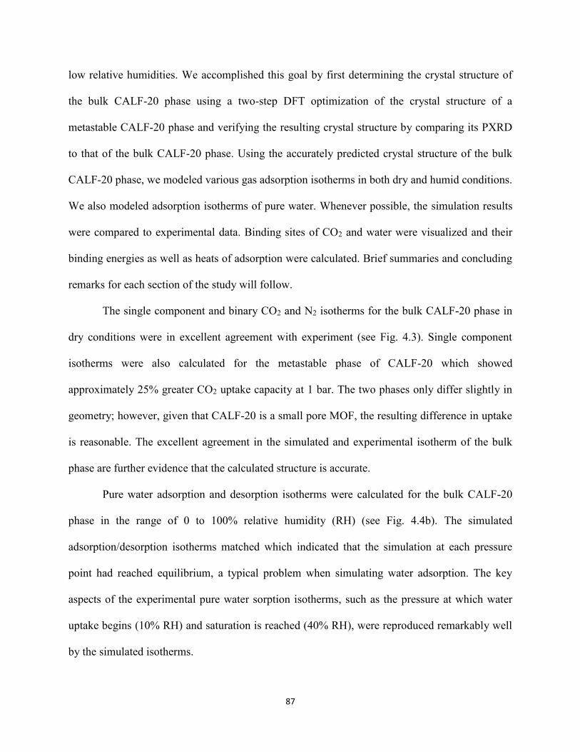
87
low relative humidities. We accomplished this goal by first determining the crystal structure of
the bulk CALF-20 phase using a two-step DFT optimization of the crystal structure of a
metastable CALF-20 phase and verifying the resulting crystal structure by comparing its PXRD
to that of the bulk CALF-20 phase. Using the accurately predicted crystal structure of the bulk
CALF-20 phase, we modeled various gas adsorption isotherms in both dry and humid conditions.
We also modeled adsorption isotherms of pure water. Whenever possible, the simulation results
were compared to experimental data. Binding sites of CO2 and water were visualized and their
binding energies as well as heats of adsorption were calculated. Brief summaries and concluding
remarks for each section of the study will follow.
The single component and binary CO2 and N2 isotherms for the bulk CALF-20 phase in
dry conditions were in excellent agreement with experiment (see Fig. 4.3). Single component
isotherms were also calculated for the metastable phase of CALF-20 which showed
approximately 25% greater CO2 uptake capacity at 1 bar. The two phases only differ slightly in
geometry; however, given that CALF-20 is a small pore MOF, the resulting difference in uptake
is reasonable. The excellent agreement in the simulated and experimental isotherm of the bulk
phase are further evidence that the calculated structure is accurate.
Pure water adsorption and desorption isotherms were calculated for the bulk CALF-20
phase in the range of 0 to 100% relative humidity (RH) (see Fig. 4.4b). The simulated
adsorption/desorption isotherms matched which indicated that the simulation at each pressure
point had reached equilibrium, a typical problem when simulating water adsorption. The key
aspects of the experimental pure water sorption isotherms, such as the pressure at which water
uptake begins (10% RH) and saturation is reached (40% RH), were reproduced remarkably well
by the simulated isotherms.

88
Next, adsorption of a gas mixture containing CO2, N2 and H2O at 293 K was modeled
where the ratio of CO2:N2 and was kept at 20:80 with a total pressure of 1 bar, and the amount of
H2O was ranged from 0.002338 to 0.02338 bar which corresponds to 10-100 % relative humidity
at 293 K (see Fig. 4.4c). This simulation showed a key feature of CALF-20, which is the
preferential adsorption of CO2 at low relative humidities (up to around 40% RH) and the
displacement of CO2 by water which results in the MOF being water-saturated at 50% RH. This
simulation was in agreement with CO2 breakthrough experiments performed on CALF-20 at 0,
20 and 40% RH (see Fig. 4.1).
Snapshots of CALF-20’s pores in equilibrium at 20% relative humidity revealed an
important mechanism of water adsorption in MOFs (see Fig. 4.6a,b). It is energetically
favourable for water molecules to adsorb and desorb together with neighboring water molecules
in the same or adjacent pores. This is due to water-water interactions (i.e. hydrogen bonding)
being stronger than water-MOF interactions.
Lastly, binding energy analysis showed that an isolated CO2 in the MOF is more strongly
bound to the MOF framework compared to an isolated H2O in the MOF (see Table 4.3). This
explains the preferential adsorption of CO2 at low relative humidities which is primarily due to
the stronger van der Waals interactions between CO2 and the MOF framework. In the high
relative humidity range, a sharp increase in water uptake is observed as a result of the strong
cooperative hydrogen-bonding effects between the adsorbed water molecules. At high relative
humidities, the binding energy per H2O (comprised of water-MOF and water-water interactions)
is higher than that of CO2. The CO2 guest binding energy also has contributions from CO2-MOF
and CO2-CO2 interactions but the latter is weaker in the case of CO2. Although CO2-MOF

89
interactions are stronger than water-MOF interactions, the strength of water-water interactions at
high relative humidities renders it more energetically favourable for water to displace CO2.
4.6 References
1. Wilcox, J. Carbon Capture; Springer. 2012.
2. 2015 Paris agreement under the United Nations framework convention on climate change;
http://ec.europa.eu/clima/policies/international/negotiations/paris.
3. B. Smit, J. A. Reimer, C. M. Oldenburg, I. C. Bourg. Introduction to Carbon Capture and
Sequestration; Imperial College Press. 2014.
4. Nicholls, R. J.; Cazenave, A. Science 2010, 328, 1517.
5. McLaughlin, J. F.; Hellmann, J. J.; Boggs, C. L.; Ehrlich, P. R. Proc. Natl. Acad. Sci. U.
S. A. 2002, 99, 6070.
6. Chung, Y. G.; Gómez-Gualdrón, D. A.; Li, P. Sci. Adv. 2016, 2, 1.
7. Folger, P. Carbon Capture : A Technology Assessment. Congressional Research Service.
2010.
8. Herm, Z. R.; Swisher, J. A.; Smit, B.; Krishna, R.; Long, J. R. J. Am. Chem. Soc. 2011,
133, 5664.
9. Kanniche, M.; Gros-Bonnivard, R.; Jaud, P.; Valle-Marcos, J.; Amann, J.-M.; Bouallou,
C. Appl. Therm. Eng. 2010, 30, 53.
10. Rochelle, G. T. et al. Science 2009, 325, 1652.
11. Vaidhyanathan, R. et al. Science 2010, 330, 650.
12. Ho, M. T.; Allinson, G. W.; Wiley, D. E. Ind. Eng. Chem. Res. 2008, 47, 4883.
13. Kresse, G. et al. VASP the GUIDE. 2009.
14. Perdew, J. P. et al. Phys. Rev. Lett. 1996, 77, 3865.

90
15. Campañá, C.; Mussard, B.; Woo, T. K. J. Chem. Theory Comput. 2009, 5, 2866.
16. Mayo, S. L. et al. J. Phys. Chem. 1990, 94, 8897.
17. Rappe, A. K. et al. J. Am. Chem. Soc. 1992, 114, 10024.
18. García-Sánchez, A. et al. J. Phys. Chem. C 2009, 113, 8814.
19. Horn, H. W. et al. J. Chem. Phys. 2004, 120, 9665.
20. Myers, A. L.; Prausnitz, J. M. AIChE J. 1965, 11, 121.

91
5 Modeling CH4 and N2 adsorption in the Ni-BPM MOF
Containing Residual Solvent
This chapter discusses simulations performed on a new MOF, Ni-BPM, synthesized using
Ni(OAc2) and 1,1′-methylenebis(3,5-dimethyl-1H-pyrazolyl-4-carboxylic acid) (H2BPM) by
Charlie Kivi in the Song group at the University of Toronto. After activation Ni-BPM retains 10
residual solvent (DMSO) molecules per unit cell in unknown locations. Our computational
screening identified Ni-BPM is a candidate material for coal mine methane purification and my
role in this collaborative study was to perform all of the computational simulation to investigate
the effects of residual solvent on gas adsorption and analyze the results. The tasks included
performing a molecular dynamics (MD) simulation to assess the mobility of the DMSO
molecules under experimental conditions, grand canonical Monte Carlo (GCMC) simulations of
CH4 and N2 uptake in the presence and absence of DMSO, detailed binding site analysis for the
guests in the framework, and binding energy calculations for CH4 and DMSO.
5.1 Abstract
The drainage gas released from coal and surrounding rock strata prior to and after coal
mining contains over 30% methane, which is a potent greenhouse gas and a possible energy
source.1 The most valuable use for this methane is to purify it to 95% by removing N2 and sell it
as pipeline quality gas or liquefied natural gas.2 MOFs are ideal candidate materials for
performing CH4/N2 separation via the pressure swing adsorption (PSA) method because its
regeneration requires less energy compared to other solid sorbents such as zeolites.3 Ni-BPM
synthesized using Ni(OAc2) and 1,1′-methylenebis(3,5-dimethyl-1H-pyrazolyl-4-carboxylic
acid) (H2BPM) is a candidate MOF material for this application, and upon activation, it retains
10 residual dimethylsulfoxide (DMSO) solvent molecules per unit cell in unknown locations.
The goal of this study is to use computational simulations to investigate the effects of residual
solvent on Ni-BPM’s CH4 and N2 adsorption properties. Single crystal X-ray diffraction
(SCXRD) data shows that there are two sets of positions (Set 1 and 2) that can be occupied by
DMSO’s in the Ni-BPM framework. Grand canonical Monte Carlo (GCMC) simulations of CH4
and N2 uptake in Ni-BPM reveal that CH4 uptake is in closest agreement with experiment when

92
the 10 DMSO’s are placed among the two sets of positions in equal ratio (Mixed Set). The CH4
binding sites within the Ni-BPM framework were found to overlap with the Set 1 DMSO
positions which explained the severe under-prediction of CH4 uptake for Ni-BPM containing
DMSO’s in Set 1 positions. Binding energy calculations indicate that CH4 molecules are most
stabilized when the DMSO’s are in the Mixed Set of positions. In this work, a variety of
molecular simulation techniques are used to show that the positions of the DMSO molecules in
Ni-BPM have a significant effect on the MOF’s CH4 uptake.
5.2 Introduction
Coal mine methane, which refers to the methane released from coal and surrounding rock
strata prior to, during and after mining operations, represents approximately 8% of the world’s
anthropogenic methane emissions that constitute a 17% contribution to total anthropogenic
greenhouse gas emissions.4 A typical mine emits methane in three streams: (1) mine ventilation
air (0.1-1% CH4), (2) gas drained from the seam before mining (60-95% CH4), and (3) gas
drained from worked areas of the mine (30-95% CH4).2 To mitigate methane emissions, most
mines flare drainage gas into the atmosphere to release it as CO2, a significantly less potent
greenhouse gas compared to methane. While flaring mitigates methane emissions, it is wasting
methane which is a potentially valuable fuel source. To reduce this waste, drainage gas can be
utilized in a number of industrial production processes such as gas turbines to generate power as
long as the methane concentration is over 30% and the supply is continuous. Many internal
combustion engines commonly use medium-quality gas.5 As such, the Appin coal mine in
Australia uses drainage gas to power 54 one-megawatt Caterpillar spark-fired engines.2 Recently,
it has been shown that a higher value application for the drainage gas is to purify the methane to
a concentration suitable for sale as pipeline quality gas or liquefied natural gas (95% purity)
93
assuming an industrial consumer is located near the mine. Since air is the major contaminant of
drainage gas, coal mine methane purification involves performing a CH4/N2 separation.
Several technologies have been considered for CH4/N2 separation including liquid
sorbents, cryogenic separation, membrane separation and pressure swing adsorption (PSA) using
solid sorbents. Liquid sorbents such as di-ethylamine (DEA) and potassium carbonate are
commonly used in the natural gas processing industry to remove surplus carbon dioxide from the
raw natural gas.6 The technology of selective absorption using liquid sorbents is therefore
mature; however, when considered for CH4/N2 separation, it was shown to be not suitable due to
the low solubility of N2 in the solvents. Cryogenic CH4/N2 separation involves a sequence of
compression, flash vaporisation and heat exchange stages to cool the gas stream until it liquefies,
then uses a distillation separator to separate a nitrogen-rich gas stream from a methane-rich
liquid stream.7 Cryogenic separation is an effective technology for performing CH4/N2 separation
but it is highly energy intensive due to the requirement of extremely low temperatures.
Membrane separation operates by maintaining a high feed pressure on one side of the membrane
and a low production pressure on the other side. The membrane suitable for performing CH4/N2
separation would have a certain pore size which allows methane to pass through while allowing
only minimal amounts of nitrogen to pass through. The major limitation of membrane
technology is in the scaling of the membrane modules. Since any damage to the membrane
would require the entire module to be replaced, the size of the modules is limited to minimize the
risk of damage due to the pressure differential. PSA using porous solid sorbents is a promising
technology for drainage gas purification due to its low energy requirements and cost advantages.
Adsorption in solid sorbents is driven primarily by physical guest-host interactions and the
regeneration of the material requires less energy. Wide-pore carbon molecular sieves are an

94
example of solid sorbents being considered for CH4/N2 separation. Metal organic frameworks
(MOFs), which are nanoporous crystalline solids composed of a network of metals and organic
linkers, are also ideal candidate materials for this purpose due to their high internal surface area
and the tunability of their pores.
This thesis chapter discuses a joint experimental and computational study of a candidate
MOF material for coal mine methane purification, Ni-BPM, synthesized using Ni(OAc2) and
1,1′-methylenebis(3,5-dimethyl-1H-pyrazolyl-4-carboxylic acid) (H2BPM). A unique aspect of
this MOF is that, upon activation, it retains 10 residual dimethylsulfoxide (DMSO) solvent
molecules per unit cell in unknown locations. Performing gas adsorption simulations on an
experimentally synthesized MOF containing residual solvent molecules can be complicated due
to the uncertainties introduced by the placement of the solvent molecules in the framework and
their unknown effects on gas uptake. Understanding the effects of residual solvent on gas uptake
is crucial to studying the CH4/N2 separation properties of Ni-BPM. Furthermore, demonstrating
the use of several simulation methods for this special case can be valuable for future gas
adsorption studies dealing with incompletely activated/solvated MOF structures.
SCXRD data for Ni-BPM saturated in DMSO is used to obtain the atomic positions of
the Ni-BPM framework as well as to identify the possible locations which the DMSO molecules
may occupy in the MOF. An MD simulation of the DMSO’s in the fixed Ni-BPM framework is
performed to assess the mobility of the DMSO’s under the conditions of gas adsorption
experiments (2 bar, 298 K). GCMC simulations of CH4 and N2 adsorption isotherms are
performed on the MOF with DMSO’s in various sets of positions to investigate the effect of
DMSO positions on gas uptake. ABSL will be used to locate the binding sites of CH4 and N2 in
Ni-BPM in the presence and absence of DMSO molecules. The binding energies of CH4 in Ni-
95
BPM containing DMSO’s in various positions will be calculated to give insight into the effects
of DMSO positions on CH4 uptake. Binding energies of DMSO will also be calculated to
investigate their preference for certain positions in the MOF framework.
5.3 Computational Details
This section provides details regarding the computational methods utilized in this project.
For information on the background theory of these methods, the reader is referred to Chapter 2 of
the thesis. For the molecular dynamics (MD) simulations of DMSO molecules in the Ni-BPM
framework, we first generated a geometry optimized DMSO molecule using the Gaussian
quantum chemistry package.8 For this optimization, the B3LYP level of theory was used with the
aug-cc-pVDZ basis set. The structural details of the optimized DMSO molecule are shown in
Table 5.1 and the atomic labels are shown in Fig. 5.1. The MD simulations were performed using
DL_POLY9 with a time step of 1 fs with a total of 100,000 equilibration steps and 1,000,000
production steps. This gave a simulation of 1 ns in length. The cut-offs for the short-range
potentials was chosen to be 10 Å.
The positions of atoms in the Ni-BPM structure were taken from SCXRD data. The
Lennard-Jones (LJ) potentials were used to model the van der Waals non-bonding steric and
dispersion interactions and the partial atomic charge approximation with Ewald summations were
used for the long-range electrostatic interactions. The LJ parameters for the MOF framework
were taken from the DREIDING force field10 and the partial atomic charges were calculated
using the REPEAT method.11 The REPEAT method used density functional theory (DFT)
gauge-modified electrostatic potential calculated using VASP12 with the PBE13 functional with a
planewave cut-off a 520 eV. The LJ parameters for CH4 and N2 guest molecules were taken from

96
the CH4-TraPPE14 and N2-TraPPE15 force fields. The LJ parameters for the DMSO molecules
were taken from the UFF force field.16 The gas adsorption simulations for a 1:1 binary gas
mixture of CH4 and N2 were carried out isothermally at 298 K. Adsorption and desorption
pressures were 2 bar and 0.2 bar, respectively. The gas adsorption simulation conditions used in
this work were taken from Li et al.3 The GCMC simulations were run for 1,000,000 equilibration
steps and 15,000,000 production steps.

97
Table 5.1: Charges and structural details of the optimized DMSO molecule.
Atom Charge (e) Bond Bond Length
O(3) -0.4633 C(1)-S(2), C(4)-S(2) 1.841
S(2) 0.2378 S(2)=O(3) 1.540
C(1), C(4) -0.2257 C(1)-H(9),
C(4)-H(5)
1.098
H(5), H(9) 0.0883 C(1)-H(8), C(4)-H(6) 1.096
H(6), H(8) 0.1270 (1)-H(10), C(4)-H(7) 1.097
H(7), H(10) 0.1231
Angle Angle Degree Dihedral Dihedral Degree
C(1)-S(2)-O(3) 106.03 C(1)-S(2)-O(3)-C(4) 108.90
64.22
-176.61
C(4)-S(2)-C(1) 96.85 C(1)-S(2)-C(4)-H(5)
H(5)-C(4)-S(2),
H(9)-C(1)-S(2)
109.56 C(1)-S(2)-C(4)-H(6)
H(6)-C(4)-2(2),
H(8)-C(1)-S(2)
106.31 C(1)-S(2)-C(4)-H(7) -57.96
H(7)-C(4)-2(2),
H(10)-C(1)-S(2)
108.57 O(3)-S(2)-C(1)-H(8) 67.71
O(3)-S(2)-C(1)-H(9) -173.12
O(3)-S(2)-C(1)-H(10) -50.94

98
Figure 5.1: The structure of the DMSO molecule with the atomic labels.
5.4 Results
This section begins with the SCXRD data for the Ni-BPM MOF showing the possible
positions for the DMSO molecule to occupy in Ni-BPM. Next, the results for the computational
study of Ni-BPM are presented in three subsections. The first subsection discusses molecular
dynamics simulations of DMSO molecules in the Ni-BPM framework to investigate their
mobility during gas adsorption experiments. The second section provides results for the grand
canonical Monte Carlo (GCMC) simulations of CH4 and N2 uptake in Ni-BPM along with
probability distributions of the guest binding sites in the MOF with and without DMSO
molecules. The last two subsections pertain to binding energy calculations and analysis for CH4
and DMSO in Ni-BPM.
5.4.1 Single Crystal X-Ray Diffraction (SCXRD) Data
Figure 5.2 shows the positions of solvent DMSO molecules in one unit cell of the Ni-
BPM framework obtained from SCXRD experiments performed at 77 K. In one unit cell, there
are two sets of 16 symmetrically equivalent positions for the DMSO molecules: Set 1 (Fig. 5.2a)
and Set 2 (Fig. 5.2b). Each of these positions has an occupancy of 0.5 indicating that the

99
probability of a DMSO molecule occupying each of these positions is 50%. The DMSO
molecules in the two sets interact with different regions of the framework walls. The SCXRD
experiment was performed on a DMSO-saturated Ni-BPM, thus the number of DMSO molecules
seen in SCXRD data is not the amount of DMSO remaining in the activated Ni-BPM. The
amount of residual DMSO was determined experimentally using thermal gravimetric and
elemental analysis to be 0.6 DMSO molecules per nickel centre which is equivalent to 9.6
DMSO molecules per unit cell. This number will be approximated as 10 for the purposes of this
study.

100
Figure 5.2: The DMSO-saturated Ni-BPM unit cell containing 16 solvent DMSO molecules in
two sets of symmetrically equivalent positions a) Set 1 and b) Set 2. Sulfur atoms of the DMSOs
are represented by yellow spheres.
5.4.2 Computational Results
5.4.2.1 Molecular Dynamics Simulation of DMSO Molecules in Ni-BPM
Molecular dynamics simulations of 10 DMSO molecules in Ni-BPM were performed at 2
bar and 298 K for 1.2 ns in order to determine whether they are mobile during the gas adsorption
experiments. The geometry of the DMSO molecules were optimized prior to being placed in the
MOF, and the atomic coordinates of the framework atoms were kept fixed throughout the

101
simulation. Traces of the trajectory of the DMSO molecules are shown in Figure 5.3. The DMSO
molecules showed some movement about their original positions, but within the duration of the
simulation, they did not migrate to different sites in the MOF. This shows that the DMSO
molecules are generally fixed at their sites in the MOF framework under the experimental
conditions. Given this insight, the positions of DMSO molecules were kept fixed for all gas
adsorption simulations performed in this work.
Figure 5.3: Superimposed snapshots of the trajectory of 10 DMSO molecules in the MOF at 2
bar and 298 K. The DMSO solvent molecules remain close to their original positions and do not
migrate to different regions of the unit cell.

102
5.4.2.2 Gas Adsorption Simulations of CH4 and N2 in Ni-BPM
After activation of Ni-BPM, 10 DMSO solvent molecules remain in each unit cell of the
MOF. Since the exact positions of these DMSO molecules are unknown, various sets of positions
were considered based on the SCXRD data to prepare the DMSO-containing Ni-BPM structures
to perform CH4 and N2 adsorption isotherms using GCMC. Cases that were considered were: i)
10 DMSO molecules randomly chosen from among the 16 Set 1 positions (Fig 5.2 a), ii) 10
DMSO molecules randomly chosen from among the 16 Set 2 positions (Fig 5.2 b), iii) 5
DMSO’s randomly picked from each set of positions (Mixed Set 1), iv) same as case iii but with
different DMSO’s picked from each set of positions (Mixed Set 2) and v) no DMSO’s in the
framework. For each case described above, single and binary gas adsorption isotherms were
calculated for CH4 and N2 at 298 K in the pressure range of 0.001 to 2 bar using GCMC. A 1:1
binary gas mixture of CH4 and N2 was used for the binary gas adsorption isotherms. The
simulated and experimental single component isotherms for CH4 and N2 are presented in Figure
5.4a) and the simulated binary gas isotherms are presented in Figure 5.4b) along with
experimental IAST-derived binary CH4 and N2 isotherms.
The isotherms show that the positions of the DMSO’s in Ni-BPM have a significant
effect on CH4 uptake and a small effect on N2 uptake. For the single component isotherms shown
in Figure 5.4a), Ni-BPM containing DMSO’s in Set 1 and Set 2 positions yielded CH4 isotherms
which severely underpredicted and overpredicted the experimental CH4 isotherm, respectively.
Both of the mixed sets yielded CH4 isotherms in excellent agreement with experiment, and
unexpectedly, so did the case with no DMSO’s (see section 5.4.2.3 for explanations). The same
trends were observed for N2 but the deviations from experiment were less pronounced. For the
binary gas isotherms shown in Figure 5.4b), the simulated CH4 isotherms followed the same

103
trends as for the single component isotherms. For the simulated N2 isotherms, a general
overprediction resulted in the case with DMSO’s in Set 1 positions giving the isotherm in best
agreement with experiment.

104
Figure 5.4: a) Single component and b) binary gas CH4 and N2 adsorption isotherms obtained
experimentally (Expt.) and through simulation (Sim.) for Ni-BPM at 298 K. The binary gas
experimental isotherms were derived from single component experimental isotherms using
IAST.

105
In order to investigate why the DMSO’s in Set 1 positions significantly decrease CH4
uptake while the DMSO’s in Set 2 positions have the opposite effect, preferred binding sites for
CH4 in the empty MOF were determined using GCMC calculations. Figure 5.5 a) – d) show
probability density plots for the adsorbed CH4 and N2 molecules in DMSO-less Ni-BPM
calculated at 2 bar and 298 K. Each CH4 binding site indicated by a circle has another CH4
binding site behind it in the unit cell. There are a total of 16 CH4 binding sites per unit cell. As
shown in Fig. 5.5 d), N2 prefers to occupy similar sites in the MOF as CH4; however, the
preference for these sites is not as strong.

106
Figure 5.5: The probability-density plots for CH4 viewed along the a) b-c, b) a-c, and c) a-b
planes and d) the probability-density plot for N2 viewed along the b-c plane in Ni-BPM in
absence of DMSO molecules. There are a total of 16 CH4 binding sites per unit cell. Circles
indicate that there are two binding sites overlapping in that particular view.
The CH4 binding sites in the absence and presence of DMSO molecules are compared in
Figures 5.6a) - d). Figure 5.5a) shows CH4 binding sites in the absence of DMSO and Figures
5.6b) - c) show CH4 binding sites in the presence of 10 DMSO molecules in their Set 1 (case i),
Set 2 (case ii) and Mixed Set 1 (case iii) positions, respectively. Figures 5.6a) and b) reveal an
interesting insight. The Set 1 DMSO positions are in fact superimposed on the preferred CH4
binding sites. Since there are 10 DMSOs in the unit cell, in this configuration, 10 of the 16 CH4
binding sites are taken up by a DMSO molecule as shown in Fig. 5b). This explains the
significantly lower CH4 uptake predicted for the MOF containing DMSO in their Set 1 positions.

107
On the other hand, the DMSO molecules in Set 2 positions do not occupy any of the CH4 binding
sites, thus allowing CH4 to occupy all 16 of their binding sites. This explains why methane
uptake is enhanced when the DMSO’s are in their Set 2 positions as opposed to Set 1 positions.
The DMSO’s in Set 2 positions not only do not block the CH4 binding sites, but also enhance
CH4 adsorption by providing favourable dispersion interactions. Figure 5.6d) shows CH4 binding
sites in the presence of DMSO molecules in their Mixed Set 1positions (case iii). In this case, 5
of the 16 CH4 binding sites are occupied by DMSO molecules but the remaining 11 sites are still
available for CH4. Therefore, it is reasonable for the gas adsorption simulations for Ni-BPM
containing DMSO’s in their Mixed Set 1 and 2 positions to give CH4 uptake that is
approximately an average of those calculated for Ni-BPM with DMSO’s in Set 1 and Set 2
positions (see Fig. 5.3). As for N2, since its uptake is significantly less compared to CH4, the
effects of the DMSO molecules and their positions are much less pronounced.

108
Figure 5.6: Probability-density plots of the CH4 uptake in the framework with a) no DMSO’s, b)
10 DMSO’s in Set 1 positions, c) 10 DMSO’s in Set 2 positions and d) 5 DMSO’s from each of
Set 1 and Set 2 positions at 2 bar and 298 K. Sulfur atoms are represented by yellow spheres.
5.4.2.3 CH4 Binding Energies in Ni-BPM
In order to compare the strength of CH4 binding in the Ni-BPM framework containing
DMSO molecules in various sets of positions (cases i - iv), CH4 binding energy was calculated
using VASP, and the results are given in Table 5.2. Equation 5.1 shows the binding energy of
each CH4 molecule defined as,
𝐸𝐵𝑖𝑛𝑑𝑖𝑛𝑔/𝐶𝐻4 =𝐸𝐹𝑊𝐾+𝐷𝑀𝑆𝑂+𝐶𝐻4−(𝐸𝐹𝑊𝐾+𝐷𝑀𝑆𝑂+𝑛𝐶𝐻4𝐸𝐶𝐻4)
𝑛𝐶𝐻4 5.1

109
where 𝐸𝐹𝑊𝐾+𝐶𝐻4+𝐷𝑀𝑆𝑂 is the potential energy of the framework containing CH4 and DMSO
molecules (if present), 𝐸𝐹𝑊𝐾+𝐷𝑀𝑆𝑂 is the potential energy of the framework with DMSO
molecules, 𝐸𝐶𝐻4 is the potential energy of one CH4 molecule and 𝑛𝐶𝐻4 is the number of CH4
molecules in the unit cell at the respective pressure. As shown in Table 5.2, CH4 binding energy
is weakest in the MOF that contains 10 DMSO molecules in their Set 1 positions (-10.24
kJ/mol). This is reasonable given that in this configuration, the regions of the MOF which
interact most favourably with CH4 molecules are occupied by DMSO molecules in their Set 1
positions. As a result, the CH4 isotherm for this MOF was severely underpredicted (see Fig. 5.3).
With 10 DMSO molecules in their Set 2 positions, the CH4 binding energy is significantly
stronger (-27.66 kJ/mol). Since the DMSO’s in Set 2 positions do not occupy the CH4 binding
sites, CH4 molecules can interact favorably with the framework in their preferred binding sites.
Furthermore, the CH4 binding energy in the MOF with DMSO molecules in their Set 2 positions
are stronger than in the MOF with no DMSO molecules (-27.66 kJ/mol vs. -24.99 kJ/mol) which
indicates that the DMSOs in their Set 2 positions stabilize the CH4 molecules through favourable
dispersion interactions. As for the MOF containing a mixed set of DMSO’s (Mixed 1), the CH4
binding energy was similar to that of Set 2 but slightly more negative (-29.43 kJ/mol) which
indicates that the combination of having five DMSOs from each set gives the best stabilizing
effect for CH4. Despite having the most negative binding energy, the DMSO’s in the mixed set
occupy 5 of the CH4 binding sites and as more CH4 molecules are adsorbed, steric repulsions
increase. As a result, the CH4 uptake for the MOF with only the Set 2 DMSO’s was higher than
for the mixed case (see Fig. 5.3). In comparison to the experimental CH4 isotherm, the MOF
containing the mixed set of DMSO’s gave the best agreement which suggests that the 10
DMSO’s in the experimental MOF are indeed a mixed set containing both Set 1 and Set 2

110
DMSO’s. Lastly, the MOF containing no DMSO’s had a CH4 binding energy of -24.99 kJ/mol
which is neither the most stable nor the least stable. This is reasonable given the absence of both
unfavourable (steric) and favourable (dispersion) interactions between the CH4 and DMSO
molecules. The canceling out of these effects coincidentally resulted in a CH4 adsorption
isotherm which was close to experiment.
Table 5.2: Comparison of relative CH4 binding energies in the MOF containing no DMSO
molecules, 10 DMSO molecules in Set 1 and Set 2 positions, and 10 DMSO molecules in a
mixed set of positions (Mixed Set 1) at 298 K and 2 bar.
No DMSO 10 DMSO in Set
1
10 DMSO in Set
2
10 DMSO in
Mixed Set 1
𝑬𝑩𝒊𝒏𝒅𝒊𝒏𝒈/𝑪𝑯𝟒 (kJ/mol) -24.99 -10.24 -27.66 -29.43
5.4.2.4 DMSO Binding Energies in Ni-BPM
Binding energies for DMSO were calculated for both sets of DMSO positions (Set 1 and
2) as well as for the mixed set (Mixed Set 1). These binding energies were determined using
single point energy VASP calculations and the calculated DMSO binding energies are
summarized in Table 5.3. Equation 5.2 shows the binding energy of each DMSO molecule
defined as,
𝐸𝐵𝑖𝑛𝑑𝑖𝑛𝑔/𝐷𝑀𝑆𝑂 =𝐸𝐹𝑊𝐾+𝐷𝑀𝑆𝑂−(𝐸𝐹𝑊𝐾+ 𝑛𝐷𝑀𝑆𝑂𝐸𝐷𝑀𝑆𝑂)
𝑛𝐷𝑀𝑆𝑂 5.2
where EFWK+DMSO is the potential energy of the framework containing DMSO molecules, EFWK,
is the potential energy of the empty framework, EDMSO is the potential energy of the isolated
DMSO molecules, and 𝑛𝐷𝑀𝑆𝑂 is the number of DMSO’s in the unit cell. The binding energies

111
per DMSO summarized in Table 5.3 suggest that it is more energetically favourable for the
DMSOs to occupy their Set 2 positions. For the Mixed Set, the binding energy per DMSO
molecule is in between the values calculated for both sets, but slightly more negative than the
mathematical average of the two. This shows that there may be some favourable cooperative
interactions between the neighboring DMSO molecules in the mixed set. Considering the
binding energies alone, they indicate that the DMSO molecules should be in Set 2 positions;
however, the simulated CH4 and N2 adsorption isotherms indicate that the DMSO molecules are
likely in the mixed set of positions. Therefore, there may be other effects at play. More studies
are needed to give a more definite answer to this question.
Table 5.3: Comparison of relative DMSO binding energies in the MOF containing 10 DMSO
molecules in Set 1 and Set 2 positions, and 10 DMSO molecules in a mixed set of positions
(Mixed Set 1) at 298 K and 2 bar.
10 DMSO in Set 1 10 DMSO in Set 2 10 DMSO in Mixed Set 1
𝑬𝑩𝒊𝒏𝒅𝒊𝒏𝒈/𝑫𝑴𝑺𝑶(kJ/mol) -43.48 -88.70 -64.24
5.5 Conclusions
Ni-BPM synthesized by the Song group contained 10 residual DMSO molecules per unit
cell upon activation. SCXRD data showed there are two sets of 16 equivalent positions for the
solvent DMSO molecules in the MOF framework (Set 1 and Set 2), where each position has an
occupancy of 0.5. First, a molecular dynamics simulation of the DMSO molecules showed that
they are relatively immobile in their positions and do not migrate to other parts of the MOF
under experimental conditions of 2 bar and 298 K. Next, gas adsorption isotherms for a 1:1
binary gas mixture of CH4 and N2 were calculated for the MOF containing various sets of 10

112
DMSO molecules (cases i – iv) and for the MOF with no DMSO molecules (case v). The various
placements of DMSOs in the unit cell gave significantly different CH4 adsorption isotherms and
slightly different N2 adsorption isotherms. The closest agreement to experiment was obtained for
the MOF containing DMSOs in two mixed sets of positions (Mixed Set 1 and 2) which combined
5 DMSO’s from Set 1 and 5 DMSO’s from Set 2. The two mixed sets gave essentially the same
CH4 adsorption isotherm which indicated that CH4 adsorption is dependent on the relative
proportion of the DMSOs in each set of symmetry distinct sites and not on the particular
positions of DMSO’s in each set of sites. Binding site analysis revealed that DMSO’s in Set 1
positions occupy the CH4 binding sites in the MOF which explained the under-prediction of CH4
uptake by the MOF containing DMSO’s in Set 1 positions. On the contrary, DMSO’s in Set 2
positions do not occupy the CH4 binding sites and enhance CH4 uptake through favourable
dispersion interactions. CH4 binding energy calculations revealed that CH4 is most stable in the
presence of DMSOs in the mixed set of positions.
This study showed that the positions of residual DMSO solvent molecules in Ni-BPM
have a significant effect on gas adsorption properties of the MOF including CH4 uptake and CH4
binding energies. The results of this study indicate that care must be taken in determining a
proper set of solvent positions in the MOF prior to performing gas adsorption simulations.
Furthermore, this study demonstrated the use of various molecular simulation techniques,
namely MD, GCMC and ABSL, to study gas adsorption properties of an incompletely activated
MOF structure. The methodologies used in this work can be applied for future gas adsorption
studies dealing with similar cases.

113
5.6 References
1. US EPA. Coal Mine Methane Recovery: A Primer. 2009.
2. Su, S. et al. Progress in Energy and Cmbustion Science. 2005, 31, 123.
3. Li, Q. et al. J. Porous Mater. 2016, 23, 107.
4. US EPA. Assessment of the worldwide market potential for oxidizing coal mine
ventilation air methane. 2003.
5. Carothers, P. et al. Technical and economic assessment: mitigation of methane emissions
from coal mine ventilation air. 2000.
6. Austin, G. T. Shreve’s chemical process industries. 5th ed. New York: McGraw-Hill.
1984.
7. US EPA. Coalbed Methane Outreach Program Technical Options Series. 1998.
8. Gaussian 09, Revision D.01, Frisch, M. J. et al. Gaussian, Inc., Wallingford CT, 2016.
9. Smith, W. et al. DL_POLY 2.20, 2010.
10. Mayo, S. L. et al. J. Phys. Chem. 1990, 94, 8897.
11. Campañá, C.; Mussard, B.; Woo, T. K. J. Chem. Theory Comput. 2009, 5, 2866.
12. Kresse, G. et al. VASP the GUIDE. 2009.
13. Perdew, J. P. et al. Phys. Rev. Lett. 1996, 77, 3865.
14. Martin, M. G. et al. J. Phys. Chem. B 1998, 102, 2569.
15. Potoff J. J. et al. AIChE Journal. 2001, 47, 1676.
16. Rappe, A. K. et al. J. Am. Chem. Soc. 1992, 114, 10024.

114
6 Conclusion
6.1 Summary
This thesis included three distinct projects in the field of computational MOF research
focusing specifically on their gas separation applications for carbon capture and storage. The
goal of the first project discussed in Chapter 3 was to develop robust machine learning QSPR
models to predict MOF performance for pre-combustion carbon capture application using
hypothetical MOF structures in the most topologically diverse database constructed to date
(358,400 MOFs, 1166 network topologies). Previous QSPR models had been developed using
hypothetical MOF databases with significantly lower topological diversity (20 network
topologies) and despite the high predictive power displayed by these models, the applicability of
QSPR modeling MOF discovery had not been established. Therefore, the motivation behind this
work was to demonstrate the ability of QSPR models to account for the high topological
diversity displayed by MOFs in the most current database, and show that QSPR modeling can be
instrumental to current MOF research. To our knowledge, this work was the first of its kind to
develop QSPR models for MOF performance for the particular application of pre-combustion
carbon capture. Furthermore, instead of using a classification method where MOFs are labeled as
either ‘good’ or ‘bad’ for the application, we used support vector regression (SVR) models such
that the outputs are generated in terms of actual values of CO2 working capacity and CO2/H2
selectivity. Using 35,840 MOFs which make up 10% of the database, we developed five SVR
models for each target property using various combinations of geometric and AP-RDF
descriptors. We found that it was necessary to normalize the range of the AP-RDF descriptors by
the number of atoms in the MOF framework to account for the geometric and size diversity
displayed by the MOFs in the database. The models were trained using the four-fold-out cross

115
validation method, and the final models were validated on MOFs in the remaining 90% of the
database. The models built using all six geometric descriptors as well as the three AP-RDF
descriptors were determined to be best performing with excellent R2 values obtained for CO2
working capacity (R2 = 0.944) and CO2/H2 selectivity (R2 = 0.876). As such, the high predictive
power we were able to achieve with the SVR models built using the most diverse set of
hypothetical MOF database to date, suggests that QSPR modeling is indeed a powerful and
reliable tool that can significantly accelerate the discovery of high performing MOFs for pre-
combustion carbon capture.
The goal of the second project of this thesis discussed in Chapter 4 was to use molecular
simulations to explain the exceptional water-resistant properties of CALF-20, the “Magic MOF”,
developed by the Shimizu group at the University of Calgary and to determine its atomic
structure. In addition to its remarkable water-resistance under flue gas conditions, CALF-20 was
experimentally found to possess a multitude of desirable characteristics including high CO2
working capacity and selectivity, hydrothermal stability, resistance to acids, and easy
regeneration. Thus, investigating the physical and chemical features of this MOF was deemed
useful for both furthering the understanding of this MOF as well as aiding in the rational design
of other high-performing MOFs for post-combustion carbon capture. We began by predicting the
atomic positions in the crystal structure of the bulk phase of CALF-20, for which only a powder
X-ray diffraction pattern was available, using a single crystal X-ray diffraction pattern (SCXRD)
of a metastable phase of CALF-20, which was available. Using DFT calculations we obtained a
structure whose simulated PXRD pattern was an excellent match to the experimental pattern.
Using the predicted CALF-20 structure, we calculated adsorption isotherms of CO2 and N2 for
CALF-20 under dry and humid conditions which were in excellent agreement with experiment.

116
Water sorption isotherms were also simulated, and snapshots of the MOF undergoing the
simulation revealed that water molecules in a given pore adsorb and desorb together due to
hydrogen bonding. Lastly, binding sites and binding energies of CO2 and water in CALF-20
show that the preferential CO2 uptake at low relative humidities is driven by the stronger binding
energy of CO2 in the MOF, and the sharp increase in water uptake at higher relative humidities is
driven by the strong intermolecular interactions between water. This work is currently included
in a combined theoretical and experimental manuscript that is currently waiting for additional
experimental results.
The third project discussed in Chapter 5 of this thesis involved investigating the effects of
residual DMSO solvent molecules on CH4 and N2 uptake in Ni-BPM, a candidate MOF for coal
mine purification synthesized by the Song group at the University of Toronto. Since the positions
of the 10 residual DMSO molecules in the MOF were unknown, we performed gas adsorption
simulations on the MOF containing DMSO’s in various sets of positions based on SCXRD data.
The simulated CH4 and N2 isotherms were in closest agreement with experiment when the 10
DMSO’s were placed among the two sets of positions (Sets 1 and 2) in equal ratio (Mixed Set).
The CH4 binding sites within the Ni-BPM framework were found to overlap with the Set 1
DMSO positions which explained the severe under-prediction of CH4 uptake for Ni-BPM
containing DMSO’s in Set 1 positions. Binding energy calculations revealed that CH4 molecules
are most stabilized when the DMSO’s are in the Mixed Set of positions. This study showed that
the positions of residual DMSO solvent molecules in Ni-BPM have a significant effect on gas
adsorption properties of the MOF, and thus care must be taken in determining a proper set of
solvent positions prior to performing gas adsorption simulations. Further, this study
demonstrated the use of various molecular simulation techniques to study gas adsorption

117
properties of an incompletely activated MOF structure which can be applied to studies of similar
cases in the future.
6.2 Publications
6.2.1 Thesis-Related Publications
(1) Dureckova, H; Krykunov, M; Zein Aghaji, M; Woo, T.K; “Robust QSPR Models for
Recognizing MOFs with High CO2 Working Capacity and CO2/H2 Selectivitiy for Pre-
combustion Carbon Capture” Manuscript in preparation
(2) Dureckova, H; Vaidhyanathan, R; Shimizu, G.K.H; Woo, T.K; “CALF-20, the “Magic
MOF” for Post-combustion Carbon Capture” Manuscript in preparation
(3) Kivi, C.E; Gelfand, B; Dureckova, H; Ma, C; Song, D; Shimizu G.K.H; Woo, T.K;
“Potential for Coal Mine Methane Purification in New Nickel MOF” Manuscript in
preparation
6.2.2 Other Publications on Topics Not Related to Thesis Projects
(1) Dureckova, H; Woo, T.K; Udachin, K.A; Ripmeester, J.A; Alavi, S; “The Anomalous
Halogen Bonding Interactions Between Chlorine and Bromine with Water in Clathrate
Hydrates”. Faraday Discuss. 2017, 203, 61.
(2) Dureckova, H; Woo, T.K; Alavi, S; “Molecular Simulations and Density Functional
Theory Calculations of Bromine in Clathrate Hydrate Phases”. J. Chem. Phys. 2016,
144, 04450.
(3) Daff, T.D; Collins, S.P; Dureckova, H; Perim, E; Skaf, M.S; Galvao. D.S; Woo, T.K;
“Evaluation of Carbon Nanoscroll Materials for Post-combustion CO2 Capture”.
Carbon. 2016, 101, 218-225.
6.3 Future Work
6.3.1 Robust QSPR Models for Recognizing MOFs with High CO2
Working Capacity and CO2/H2 Selectivitiy for Pre-combustion
Carbon Capture
This project was the first attempt at using QSPR models to predict performance of MOFs
in the most topologically diverse database of hypothetical MOF structures known to date
(358,400 MOFs, 1166 topologies). We were successful in building two robust and accurate

118
models for predicting CO2 working capacity (R2=0.944) and CO2/H2 selectivity (R2=0.876). This
was accomplished by the use of novel y-range normalized AP-RDF descriptors which allowed
the models to capture the diverse range of geometric properties exhibited by the MOFs in the
database.
There are several different avenues that can be explored as future work in relation to this
project. First, the high-performing MOFs identified can be surveyed for common structural
features such as presence of certain SBUs, topologies and certain geometric features such as pore
sizes within a specific range. This information will be useful for aiding synthetic chemists in the
rational design of high-performing MOFs for pre-combustion carbon capture. Furthermore, a
small number of top performing MOFs identified by these models can be further studied
computationally to examine whether they meet other performance criteria such as hydrothermal
stability. Once the best high-performers have been selected, they can be proposed to synthetic
labs as potential target materials. Second, the novel y-range normalized AP-RDF descriptors can
be implemented in previously developed AP-RDF based QSPR models1–3 to examine whether
they improve their predictive power. Lastly, QSPR models for other gas separation applications
such as oxy-fuel combustion carbon capture can be developed using the same descriptors used in
this work. This will involve performing gas adsorption simulations under the particular
conditions of the application and calculating target values such as O2 working capacity and
O2/N2 selectivity. Since the codes for the SVR models have already been written, only the input
variables need to be determined. The use of MOFs in the context of oxy-fuel combustion carbon
capture is an area that has not been extensively studied due to the difficulty of separating O2 and
N2, which are very similar species in size and shape. Certain MOFs which are oxophillic (i.e.
have an affinity for O2) may have potential in this area.

119
6.3.2 Modeling CO2 and H2O Adsorption in CALF-20, the “Magic MOF”
The first part of this computational study involved predicting the crystal structure of the
bulk phase of CALF-20 from a single crystal X-ray diffraction pattern of a metastable single
crystal phase of CALF-20. This exercise revealed that given detailed structural information on a
structurally related phase, it is possible to use ab initio calculations to determine the structure of
the phase of interest given that its powder X-ray diffraction pattern is available. Furthermore, this
project outlined a methodology for simulating water uptake in MOFs using individual GCMC
simulations for each relative humidity value and using the equilibrated system as a starting point
for the next relative humidity value. This procedure can be utilized to simulate water adsorption
in other porous materials.
6.3.3 Modeling CH4 and N2 Adsorption in the Ni-BPM MOF
The motivation behind this case-study was to understand the effects of residual solvent in
the Ni-BPM MOF on its gas adsorption properties. We gained great insight into the effects of
solvent positions on gas uptake, and it became clear that the solvent positions must be chosen
accurately in order for simulations to reproduce experimental gas adsorption isotherms. In terms
of the MOF itself, the presence of residual solvent is not ideal for industrial applications. It is
difficult to predict whether the same amount of solvent will remain in the MOF for every batch
of the MOF synthesized, and therefore its performance may not be consistent. However, this
project demonstrated the use of a series of molecular simulation techniques to study the effects
of solvent positions on gas uptake. The methodology developed in this work can be applied to
studies of other systems containing residual solvent.

120
6.4 References
1. Fernandez, M.; Trefiak, N. R.; Woo, T. K. J. Phys. Chem. C 2013, 117, 14095.
2. Fernandez, M.; Boyd, P. G.; Daff, T. D.; Aghaji, M. Z.; Woo, T. K. J. Phys. Chem. Lett.
2014, 5, 3056.
3. Aghaji, M. Z. et al. Eur. J. Inorg. Chem. 2016, 4505.

121
7 Appendices
Table A1: The NIMF force field parameters for N2.
Species Atom bl (Å) q (e) (ϵ/kb) (K) σ (Å)
N2 N 0.5500 -0.4820 39.966 2.4549
COM 0.0 0.9640 0 0
H - Variable (~0.05 - 0.2) 22.142 2.5711
B - Variable (~0.2 - 0.4) 90.581 3.6375
N - Variable (~ - 0.4) 34.722 3.2607
Note: bl is distance of the atom to the molecular mass center.
Lorentz-Berthelot mixing rules were used to determining parameters between atoms of different
types.
Table A2: Comparison of Lennard-Jones parameters and partial atomic charges for TIP4P-Ew
and CO2.
Guest Species Atoms σ (Å) ε (kcal/mol) Charge (e)
CO2 C 2.745 0.05948 0.65120
O 3.017 0.17023 -0.32560
TIP4P-Ew O 3.16435 0.16275 0.00000
H (x2) ---- ---- 0.52422
Hx (dummy) ---- ---- -1.04844


