Robust Human Motion Tracking using Low-Cost Inertial ...principle of navigation systems based on...
149
Robust Human Motion Tracking using Low-Cost Inertial Sensors by Yatiraj K Shetty A Thesis Presented in Partial Fulfillment of the Requirements for the Degree Master of Science Approved November 2016 by the Graduate Supervisory Committee: Sangram Redkar, Chair Thomas Sugar Spring Berman Hyunglae Lee ARIZONA STATE UNIVERSITY December 2016
Transcript of Robust Human Motion Tracking using Low-Cost Inertial ...principle of navigation systems based on...

Robust Human Motion Tracking using Low-Cost Inertial Sensors
by
Yatiraj K Shetty
A Thesis Presented in Partial Fulfillment
of the Requirements for the Degree
Master of Science
Approved November 2016 by the
Graduate Supervisory Committee:
Sangram Redkar, Chair
Thomas Sugar
Spring Berman
Hyunglae Lee
ARIZONA STATE UNIVERSITY
December 2016

i
ABSTRACT
The advancements in the technology of MEMS fabrication has been phenomenal in recent
years. In no mean measure this has been the result of continued demand from the consumer
electronics market to make devices smaller and better. MEMS inertial measuring units
(IMUs) have found revolutionary applications in a wide array of fields like medical
instrumentation, navigation, attitude stabilization and virtual reality. It has to be noted
though that for advanced applications of motion tracking, navigation and guidance the cost
of the IMUs is still pretty high. This is mainly because the process of calibration and signal
processing used to get highly stable results from MEMS IMU is an expensive and time-
consuming process. Also to be noted is the inevitability of using external sensors like GPS
or camera for aiding the IMU data due to the error propagation in IMU measurements adds
to the complexity of the system.
First an efficient technique is proposed to acquire clean and stable data from unaided IMU
measurements and then proceed to use that system for tracking human motion. First part
of this report details the design and development of the low-cost inertial measuring system
‘yIMU’. This thesis intends to bring together seemingly independent techniques that were
highly application specific into one monolithic algorithm that is computationally efficient
for generating reliable orientation estimates. Second part, systematically deals with
development of a tracking routine for human limb movements. The validity of the system
has then been verified.
The central idea is that in most cases the use of expensive MEMS IMUs is not warranted
if robust smart algorithms can be deployed to gather data at a fraction of the cost. A low-

ii
cost prototype has been developed comparable to tactical grade performance for under $15
hardware. In order to further the practicability of this device we have applied it to human
motion tracking with excellent results. The commerciality of device has hence been
thoroughly established.

To my mother: Geeta
And
father: Krishnaraj Shetty

iii
ACKNOWLEDGMENTS
All this would have been inconceivable without the support of my parents and my brother,
I thank them for being with me always and financially supporting me throughout my
studies.
I appreciate the help I got from Osama and Eddy for hardware design, and Yuchong for his
rate table. I also thank Prof. Kannan for giving me access to his thermal chamber and Pavan
for helping me set up the experiment.
I thank Prof. Redkar for giving me this opportunity to work on such a wonderful project.
Working with him gave me inspiration and insight to look at engineering problems
critically, and confidence to work on any subject. I also thank him for the futon :)

iv
TABLE OF CONTENTS
Page
LIST OF TABLES ……………………………………………………….. vii
LIST OF FIGURES ……………………………………………………… viii
CHAPTER
1 INTRODUCTION …………………………………………………. 1
1.1 Inertial Measurement Unit ………………………………. 2
1.1.1 Operational Principle……………………………………... 3
1.1.2 Grades of IMUs…………………………………………... 5
1.1.3 Inertial Navigation System……………………………….. 7
1.1.4 System Applications ……………………………………... 9
1.2 Human Motion Tracking using Inertial Sensors …………. 10
1.2.1 Rehabilitation Studies ……………………………………. 10
1.2.2 Gait Augmentation……………………………………….. 11
1.2.3 Motion Capture…………………………………………… 13
1.2.4 Summary…………………………………………………. 14
1.3 Previous Work……….…………………………………… 16
1.3.1 Addressing the Limitations………………………………. 19
1.4 Objectives and Methodology…………………………….. 20
1.5 Outline……………………………………………………. 20
2 DEVELOPMENT OF LOW-COST INERTIAL MEASUREMENT
UNIT: yIMU……………………………………………………………..
22

v
CHAPTER Page
2.1 Error Modelling and Calibration…………………………. 24
2.1.1 Types of Errors…………………………………………... 24
2.1.2 Temperature Compensation ……………………………... 29
2.1.3 Static Bias Compensation……………………………….. 32
2.1.4 Allan Variance Analysis………………………………… 34
2.1.5 Power Spectral Density Analysis………………………… 36
2.1.6 Probability Density Function…………………………….. 37
2.1.7 Drifting Bias Analysis…………………………………… 38
2.1.8 Simplified Error Model………………………………….. 42
2.2 Dual IMU System………………………………………… 43
2.2.1 Dual IMUs……………………………………………….. 43
2.2.2 Common Mode Effect……………………………………. 45
2.3 Sensor Fusion ……………………………………………. 32
2.3.1 Representing Angles……………………………………… 48
2.3.2 Complementary Filter…………………………………….. 53
2.3.3 Sensor Fusion Scheme……………………………………. 54
2.4 Hardware Design…………………………………………. 58
2.4.1 System Design……………………………………………. 59
2.4.2 Enclosure Design…………………………………………. 61
2.5 Performance Evaluation………………………………….. 63
2.5.1 Testing Validity of Common Mode Effect……………….. 63
2.5.2 AV Results……………………………………………….. 72

vi
CHAPTER Page
2.5.3 PSD Results………………………………………………. 76
2.5.4 PDF Results………………………………………………. 78
2.5.5 Drifting Bias Analysis Results…………………………… 81
2.5.6 Orientation Tracking Performance……………………….. 84
3 JOINT ANGLE TRACKING USING INERTIAL SENSORS……. 89
3.1 Joint Angle Tracking …………………………………….. 89
3.1.1 Kinematic Modelling of Upper Limb…………………….. 89
3.1.2 Sensor-Segment Calibration……………………………… 98
3.1.3 System Design……………………………………………. 99
3.2 Performance Evaluation………………………………….. 100
3.2.1 Experiment……………………………………………….. 100
3.2.2 Results and Discussion…………………………………… 103
4 CONCLUSION…………………………………………………….. 104
4.1 Contributions…………………………………………….. 104
4.2 Future Work……………………………………………… 106
REFERENCES…………………………………………………………… 109
APPENDIX
A MATHEMATICAL RESULTS………………………….. 114
B STATIC TEST PLOTS…………………………………... 122

vii
LIST OF TABLES
Table Page
2.1 Hardware Specification Of yIMU v1.4………………………………… 59
2.2 The Results of Linear Best Fit Between Sensor Output and
Temperature for Mpu6050 in Opposing Configuration………………...
66
2.3 Accelerometer Bias Error………………………………………………. 71
2.4 Gyro Bias Error…………………………………………………............ 72
2.5 Comparing the Results of Av Analysis Between IMU-1 and yIMU
Accelerometers………………………………………………………….
74
2.6 Comparing The Results Of AV Analysis Between IMU-1 And yIMU
Accelerometers………………………………………………………….
75
2.7 PSD Slope Values For IMU-1…………………………………………. 77
2.8 PSD Slope Values For yIMU. …………………………………………. 78
2.9 IMU-1 Measurement Noise Variances………………………………… 80
2.10 yIMU Measurement Noise Variances…………………………………. 81
2.11 Markov Parameters For Single IMU-1………………………………… 82
2.12 Markov Parameters For yIMU And Comparison To yIMU…………… 83
3.1 DH Parameters For Upper Limb……………………………………….. 94

viii
LIST OF FIGURES
Figure Page
1.1 A Circuit Board Of An IMU Containing MEMS Component………… 3
1.2 Schematic Of An Inertial Measurement Unit………………………….. 3
1.3 Principle of Operation of MEMS Inertial Sensors…………………….. 4
1.4 Inertial Sensor Grades…………………………………………………. 7
1.5 MPU6050 Breakout Board…………………………………………….. 8
1.6 (A) Gimbaled Inertial Measuring Unit (B) Strapdown Inertial
Measuring Unit …………………………………………………………
9
1.7 Strapdown Inertial Navigation Computing Tasks ……………………... 11
1.8 Devices Designed to Augment Human Running Developed at Human
Machine Integration Lab, ASU ………………………….......................
12
1.9 eLegs Developed At Berkeley Robotics And Human Engineering
Lab………………………………………………………………………
13
1.10 Rendering For An Inertial Mocap By Perception Neuron…………….. 25
2.1 Static Bias Error……………………………………………………….. 26
2.2 (Left) Scale Factor Error; (Right) Misalignment Error………………… 31
2.3 Temperature Compensation……………………………………………. 32
2.4 The Bias Compensated Angular Yaw Rate for the IMUs (Z Axis)……. 33
2.5 The Bias Compensated Angular Roll Rate for the Imus (X Axis)…….. 34
2.6 The Bias Compensated Accelerometer Readings for the IMUs (X
Axis)…………………………………………………………………….
35
ix
Figure Page
2.7 Sample Allan Deviation Plot For An Accelerometer………………….. 36
2.8 PSD For A Sample Accelerometer…………………………………….. 37
2.9 Visual Representation Of Gaussian Distribution………………………. 38
2.10 Random Walk For A Sample MPU6050 Gyroscope………………….. 39
2.11 A Virtual IMU Observation Fusion Architecture……………………… 44
2.12 Dual Axes Configuration………………………………………………. 45
2.13 Gyroscope Output Comparison for Two IMUs with Opposed Sense
Axes…………………………………………………………………….
46
2.14 Gyroscope Drift for Two Imus with Opposed Sense Axes……………. 47
2.15 Euler Angle Representation……………………………………………. 49
2.16 Measuring Tilt Using Accelerometers…………………………………. 50
2.17 Measuring Angles Using Gyroscopes………………………………….. 51
2.18 Euler To Quaternion Conversion…………………………………......... 52
2.19 Complementary Filter Structure…………………………………........... 54
2.20 The Stacked Boards In yIMU v1.4…………………………………...... 60
2.21 The Sense Axes Of The Dual IMU System……………………………. 61
2.22 Enclosure For yIMU v1.4 With Straps………………………………… 62
2.23 Heraeus UT12p Thermal Chamber…………………………………...... 64
2.24 Temperature Profile Of The Experiment………………………………. 65
2.25 Sample Scatter Plot Of Acc Axis X For IMU1………………………… 65
2.26 Sample Scatter Plot Of Gyro Axis X For IMU2……………………….. 66

x
Figure Page
2.27 Comparison of Temperature Effect Trends For Gyro X of IMU1,
IMU2 And Combined Output …………………………………………
67
2.28 The FMC Shaker Used For Vibration Testing…………………………. 68
2.29 Effect Of Vibration On IMU1 Accelerometers………………………… 69
2.30 Effect Of Vibration On IMU1 Gyroscopes…………………………….. 69
2.31 Effect Of Vibration On Vibration Axis (Z axis)……………………….. 70
2.32 Effect of Vibration On Cross Axis (X axis)……………………………. 71
2.34 Allan Deviation Plot For IMU-1 Accelerometer X……………………. 73
2.35 Allan Deviation Plot For yIMU Accelerometer X…………………….. 74
2.36 Allan Deviation Plot For IMU-1 Gyroscope X………………………… 74
2.37 Allan Deviation Plot For yIMU Gyroscope X…………………………. 75
2.38 PSDs for IMU-1: (above) accelerometer (below) gyroscope for X axis. 77
2.39 PSDs for yIMU: (Above) Accelerometer (below) Gyroscope For X
Axis…………………………………………………………………….
78
2.40 IMU-1 Measurement Noise Histogram with Gaussian Pdf Plotted over
It (above) Accelerometer X (below) Gyroscope……………………….
79
2.41 yIMU Measurement Noise Histogram With Gaussian PDF Plotted
Over It (Above) Accelerometer X (Below) Gyroscope X……………..
80
2.42 Random Walk In IMU-1 GyroX………………………………….......... 82
2.43 Random Wwalk In yIMU GyroX……………………………………… 83
2.44 Tracking Testing Apparatus…………………………………................. 84
2.45 Angle Vs Time………………………………….................................... 85

xi
Figure Page
2.46 Rate Table Experiment about Yaw Axis- Constant Speed…………….. 86
2.47 Rate Table Experiment about Yaw Axis- Varying Speed …………….. 86
2.48 Static Stability of yIMU- Gyroscopes Tested for 1 Hour ……………... 87
2.49 Static Stability of Mpu6050 with Dmp Algorithm Tested for 20
Minutes…………………………………………………………………
87
2.50 Raw Gyro Output From MPU6050 For 20 Minutes…………………… 88
3.1 Movements In Human Joints…………………………………............... 89
3.2 Categories Of Joint Movements…………………………………........... 91
3.3 Visualizing Human Body As Series Of Kinematic Segments…………. 92
3.4 Kinematic Modelling Of Human Upper Limb…………………………. 94
3.5 Forward Kinematics- Frames Of Reference…………………………… 95
3.6 Sensor-Segment Calibration……………………………………………. 99
3.7 Tracking System Design………………………………………………. 99
3.8 yIMU Placement On Subject Body……………………………………. 101
3.9 Graph Comparing the Elbow Flexion Angle Calculated Using the
Noraxon IMUs with YIMU …………………………………………….
101
3.10 Graph comparing the shoulder rotation calculated using the Noraxon
IMUs with yIMU………………………………………………………..
102
3.11 Graph comparing the elbow flexion angle calculated using the
Noraxon IMUs with yIMU……………………………………………...
102
3.12 Graph comparing the knee flexion angle calculated using the Noraxon
IMUs with yIMU……………………………………………...
102

1
Chapter 1
INTRODUCTION
The main driver for increase in research activity in the field of inertial sensors applied to
human motion analysis in recent years is due to the increase in the quality of micro-electro-
mechanical systems (MEMS) technology. Being portable and cheap, MEMS based sensors
are finding extensive usage in tracking the position and orientation of human limbs. But
these inertial sensors have the nagging problem of accumulating errors over a period of
time. The low-cost IMUs currently available in the market are lacking the accuracy needed
for precision tracking applications. Hence the focus in this thesis is to develop a low-cost
IMU that could be used in motion tracking systems. The resulting device is named yIMU.
This chapter is divided into five sections:
1. In this section, we introduce the Inertial Measurement Unit and their applications.
We also delve into the background theory to further understand the working
principle of navigation systems based on inertial sensors.
2. In this section, we look into the application of inertial sensors for tracking human
motion. Bunch of concerned applications have been mentioned pointing to the
commerciality of the technology.
3. Here we survey the relevant body of literature to develop our system. The focus
was to look at the efficient techniques that could be implemented and refined to
develop a cheap, compact and accurate inertial tracking solution in a limited budget

2
and development cycle. Furthermore, the limitations in previous research are
highlighted and the suggested steps to be taken is discussed.
4. Here we state the objectives that need to be accomplished in this thesis and the
broad methodology followed is mentioned.
5. Finally, the outline of the remainder of the thesis is presented.
1.1 Inertial Measurement Unit
Given the initial position and orientation of a body, inertial sensors can be used to track the
motion of the body in time. The technique/process used is known as inertial tracking. An
Inertial Measuring Unit is a device with accelerometers and gyroscopes that are used to
measure linear accelerations and angular velocities respectively. Most IMUs even have
magnetometer to assist in aiding the orientation. These physical quantities can be integrated
over time to obtain an estimate of the positions and orientations of the body. But this
requires development of appropriate sensor fusion algorithms, to take into account the
propagation of integration errors of the sensors. But the cost and size of MEMS IMUs
render them suitable for various consumer electronics, automobiles and are especially
popular amongst hobbyists.

3
Figure 1.1: A circuit board of an IMU containing MEMS component
1.1.1 Operational Principle
Though the IMU system appears to be complicated the physics is surprisingly simple.
Angular velocity can be measured by exploiting the Coriolis Effect of a vibrating structure;
when a vibrating structure is rotated, a secondary vibration is induced from which the
angular velocity can be calculated. Acceleration can be measured with a spring suspended
mass; when subjected to acceleration the mass will be displaced. The mems technology is
used to implement these mechanical structures on silicon chips in combination with
capacitive displacement pickups and electronic circuitry.
Figure 1.2 : Schematic of an Inertial Measurement Unit (Groves 2013)

4
Accelerometers- Accelerometers theoretically measure ‘specific force’ the sum of linear
acceleration and gravity. In quasi-static situations, linear acceleration can be neglected with
respect to the gravity and sensor measurements can be used to estimate the orientation
relative to the horizontal plane. However, in a dynamic situation (free motion) the
accelerometer measures both the linear acceleration and gravity. In this case, it is not easy
to dissociate these two physical quantities, and thus, it becomes difficult to calculate the
attitude accurately.
Figure 1.3: Principle of operation of MEMS inertial sensors: (above) accelerometers
(below) gyroscopes (Groves 2013)

5
Gyroscopes- Gyroscopes measure angular velocities which can be integrated over time to
compute the sensor's orientation. Nonetheless, the integration of gyroscope measurement
errors and biases leads to an accumulating error in the calculated orientation.
Magnetometers- Magnetometers, on the other hand are used to measure the local magnetic
field vector in sensor coordinates and allow the determination of orientation relative to the
vertical axis, which provides additional information regarding orientation. The main
problem with magnetometers is the influence of magnetic interferences fixed to the sensor
frame or ferromagnetic materials around the sensor that corrupt the measurements.
1.1.2 Grades of IMUs
Based on the price and performances characteristics inertial sensors are categorized into
many grades:
1. STRATEGIC GRADE
The best among these belong to the category of strategic grade which includes
marine and navigation grade sensors. These sensors are so accurate that the system
will only drift by less than 1.8 km per day (VectorNav). But they are very expensive
with aviation grade costing around $100000 per unit with marine grade costing in
the neighborhood of a million dollars for a full system. The technology used to
create these gyroscopes are usually Ring Laser (RLGs) and Fiber Optics (FOGs).

6
Figure 1.4: Inertial sensor grades (Hol 2011)
2. TACTICAL GRADE
Tactical grade sensors are widely used in military munitions and navigation systems
for UAVs. These sensors can be used unaided for a few minutes, but with accurate
external aiding like GPS these systems can be very accurate. They usually cost tens
of thousands of dollars.
3. INDUSTRIAL GRADE
Industrial sensors are used in automobiles, medical devices and industrial
automation applications. They usually cost few hundred dollars to thousands of
dollars depending on performance.
4. CONSUMER GRADE
The lowest grade is consumer grade sensors which are usually made based on
MEMS technology making them cheap. Usually industrial grade sensors are just
better calibrated consumer grade sensors, the difference in this range is due to
sophistication of the calibration process. Consumer grade IMUs are very cheap and
could be found for less than $5.

7
Figure 1.5: MPU6050 breakout board: a consumer grade sensor used for this project
The range of inertial sensors from automotive to marine grade spans six orders of
magnitude in gyroscope performance. These divisions in performance is usually based in
the bias stability specifications. Bias stability is the measure of the variation of gyroscopic
bias with respect to time. The more stable it is, the better the IMU. Tracking estimates are
heavily dependent on the gyro performance, hence better the gyro less the errors in the
estimates.
1.1.3 Inertial Navigation System
An inertial navigation system (INS) is a navigation aid that uses a computer, motion sensors
(accelerometers) and rotation sensors (gyroscopes) to continuously calculate via dead
reckoning the position, orientation, and velocity of a moving object.
Dead reckoning- is the process of calculating the current position of a vehicle by using a
previously determined position, updating that position based upon known or estimated
speeds over elapsed time and course. Due to integration errors the calculations are prone
to being erroneous over time.
Basically an INS consists of the following:

8
An IMU or an inertial reference frame (IRF) consisting of sensors which are rigidly
mounted. This is used to measure the pose of the body.
Navigation computers to make the estimation calculations.
Figure 1.6: (a) Gimbaled inertial measuring unit (b) Strapdown inertial measuring
unit (Grewal, Weill et al. 2001)
The system design can be broadly divided into two categories:
Gimbaled systems- use a multiple gimbal framework with rotation bearings for
independent rotation of attached frames from the host vehicle. At least three
gimbals are required to isolate the system from host vehicle rotations about three
axes (roll, pitch and yaw). These systems are expensive but have very high
accuracy. This is especially useful for applications where GPS aiding is not
available e.g. in submarine navigation.
Strapdown systems- have the inertial sensor cluster rigidly mounted onto the host
vehicle. The wearable sensor systems under discussion can be categorized as
strapdown systems. These systems have much higher rotation rates than gimbaled

9
systems which requires compensation mechanisms to give accurate output. The
following flowchart shows the simplification of computing tasks involved in
calculation of pose using a strapdown inertial navigation system.
Figure 1.7: Strapdown inertial navigation computing tasks (Titterton and Weston
2004)
1.1.4 System Applications
Wide array of applications in aircraft and spacecraft navigation and attitude control
systems; missiles and other munition applications; marine navigation. Recent advances in
MEMS technology have drastically reduced the price and size of inertial sensors thereby
ushering in extensive applications in consumer electronics and automotive industry.
IMUs have a great utility advantage over other navigation sensors like GPS and magnetic
compasses in that they can be used in varying environments where those sensors cannot be
10
used. For navigation purposes IMUs are used in combination with a secondary navigation
sensor to check the growth of errors in measurements. Kalman filter is extensively used to
update the readings to generate a more accurate dead-reckoning result.
1.2 Human Motion Tracking using Inertial Sensors
Human motion tracking is a vast field with many areas under its purview. In this section,
we present a brief description of areas of research currently undergoing lot of
improvements. At the end we summarize the advantages and disadvantages of using inertial
sensors for human motion tracking.
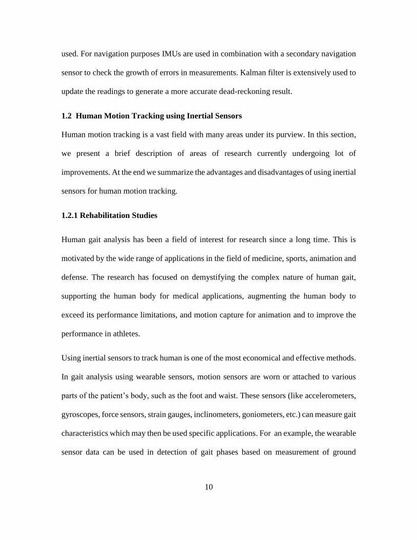
1.2.1 Rehabilitation Studies
Human gait analysis has been a field of interest for research since a long time. This is
motivated by the wide range of applications in the field of medicine, sports, animation and
defense. The research has focused on demystifying the complex nature of human gait,
supporting the human body for medical applications, augmenting the human body to
exceed its performance limitations, and motion capture for animation and to improve the
performance in athletes.
Using inertial sensors to track human is one of the most economical and effective methods.
In gait analysis using wearable sensors, motion sensors are worn or attached to various
parts of the patient’s body, such as the foot and waist. These sensors (like accelerometers,
gyroscopes, force sensors, strain gauges, inclinometers, goniometers, etc.) can measure gait
characteristics which may then be used specific applications. For an example, the wearable
sensor data can be used in detection of gait phases based on measurement of ground

11
reaction forces (Kong and Tomizuk 2009) and monitoring of human gait based on the same
principle (Zhang, Tomizuka et al. 2014).
1.2.2 Gait Augmentation
Human gait refers to the human mobility due to motion of legs. Over the course of
evolution humans have developed to have bipedal locomotion. Before the invention of
agriculture, humans have been known to be migratory species. Being bipedal allows
humans to travel large swathes of territory in an efficient manner. In fact, even in modern
era walking is more efficient than using automobile to traverse rugged terrain and in many
adverse environments.
Soldiers often need to carry heavy loads in trying physical and psychological conditions.
Over an extended period of time, a drastic reduction in degradation in efficiency and
decision making ability has been documented which could prove ominous to the mission
as well as hazardous to the soldier.
Figure 1.8: Devices designed to augment human running developed at Human
Machine Integration Lab, ASU: (from left to right) AirLegs V1, AirLegs V2 and Jet Pack
(Kerestes 2014)

12
There is a cost-effective solution to this problem- gait augmentation. The goal of gait
augmentation devices is to supply additional amounts of torque at appropriate time during
locomotion to decrease the metabolic energy consumption. This in turn would increase the
efficiency and performance of the individual i.e. increase in range, endurance and speed of
locomotion.
It is to be noted that leveraging the power available to soldiers for movement is not the
only application of gait augmentation. Disabled patients and elderly population who are in
need of walking assistance could also benefit from these devices. Proper use of these
devices may result is drastic reduction in assistance required from physical therapist
thereby reducing the cost of treatment considerably.
The HESA (Hip Exoskeleton for Support and Augmentation) is one of the exoskeleton
devices designed by Human Machine Integration Lab at *ASU that could accomplish the
above set goal. The idea is that of a device that could provide support and torque to the hip
during normal gait to reduce the metabolic cost on human body.
Figure 1.9: eLegs developed at Berkeley Robotics and Human Engineering Lab
(eLegs 2010)

13
Gait augmentation could be successfully implemented only if accurate orientation of hip
with respect to torso, i.e. angle about the pelvic joint, is known. For HESA we use two
IMUs: one mounted onto the hip and the other to the torso.
1.2.3 Motion capture
Every human gait research deals with motion capture which can be achieved by various
sensing methods: optical, mechanical, magnetic, acoustic, or inertial tracking. Although
much less expensive and more portable than marker-based optical systems, marker less
solutions are still lagging behind the more expensive systems in terms of the achieved
accuracy. A comparatively new and quickly developing frontier on human motion capture
system is based on the use of wearable sensor units comprised of magnetic and inertial
sensors that are attached to the objects in order to track their position and orientations.
Some of the most often used contemporary commercial motion tracking systems are the
Xsens, Intersense, Perception Neuron, Synertial and Trivisio.
Figure 1.10: Rendering for an inertial mocap system (PerceptionNeuron)

14
1.2.4 Summary
The overarching goal of the research is taking first step to devise a portable wireless
tracking system that is both robust and economical to be used by people to help them in
their activities. Here MEMS based inertial tracking systems lead hands down due to their
versatility and economic accessibility. But they have a bunch of limitations that needs to
be addressed before they can be effectively used in human motion tracking.
Advantages of MEMS based IMUs-
1. Light weight and portable systems.
2. Economical as the MEMS based inertial sensors are order of magnitude cheaper
than other varieties.
3. No inherent latency associated with this sensing technology and all delays are due
to data transmission and processing (Fourati, Manamanni et al. 2013).
4. No requirement of an emission source- electromagnetic, acoustic, and optic devices
require emissions from a source to track objects.
5. Enable unhindered movement of the human subject and no problem of occlusion.
6. Data collection is unrestricted by the requirement to stay in the laboratory
environment.
7. Ease of use as not many accessories are needed for setting up the tracking system.
8. Huge amount of data collection is possible i.e. from many gait cycles.
9. Using accelerometers to avoid errors related to differentiation of raw displacement
data (Kavanagh, Morrison et al. 2006).

15
10. Excellent sensitivity even for small displacements. This proves to be extremely
useful in medical diagnostics and rehabilitation.
11. Cost effective and widely available sensors
12. High sampling rate
13. Can work in total darkness (unlike optical systems) and can work in unconstrained
environments.
Notwithstanding the above advantages over other mainstream motion capture systems, the
inescapable downside is the measurement accuracy of MEMS IMUs. Their outputs are
corrupted by several high power error components. During the unaided mode of operation,
these high power error components quickly accumulate in the navigation states leading to
unacceptable navigation solutions in a very short period of time (Yuksel 2011). Also
sensors are sensitive to locations on the body and require multiple sensors for capturing
full body movements which can be annoying at times.
As we can see the errors are temporal in nature and highly dependent on the application for
which it is used. As a result, an application specific aiding source is required to correct this
propagation of measurement errors. The combination of GNSS/INS to improve the
measurement accuracy for motion capture could be done (Kwakkel 2008). GPS is well
known to give erroneous measurements over a short time span. On the other hand, INS is
reliable over short time span but degrades over an extended period of time. Hence using
the complementary characteristics of these both systems would result in a highly accurate
tracking system.

16
But if the problem is modified to not include any assistance from external sources (like
GPS), the solution will lead to an autonomous inertial tracking system. In this pursuit of
autonomous tracking system to find the relative orientation of human limbs, the application
of kinematic constraints to cap the measurement errors appears to be an apt solution.
1.3 Previous Work
Researcher working in this area have reported that due to propagation of integration errors
in inertial sensors, it is impossible to get accurate angle and displacement estimates. But
with smart signal processing techniques these errors can be reduced. Integration error
components quickly accumulate in the navigation states leading to bad tracking results in
a drift of 100- 250 after one minute and double integration of accelerometer data leads to
positional error that varies cubically with time (Roetenberg, Luinge et al. 2005).
Slifka (Slifka 2004) had developed a double integration scheme for accelerometers that
was able to measure displacement with an error of less than 10 percent. Part of the error is
inherently due to the process of numerical integration which could be further minimized
by increasing the sampling rate. But this was tested on a linearly constrained vehicle body.
Benoussaad et al (Benoussaad, Sijobert et al. 2016) devised a more elaborate method for
step height detection using double integration and drift cancellation assisted by gyroscopes.
This algorithm had error under 15% when tested on subjects walking at various speeds.
This approach did not work for extended periods of time. In addition, they did not use low
cost sensors for their applications. Whereas Barret et al (Barrett, Gennert et al. 2012) have
used consumer grade sensors to develop an improved IMU by implementing calibration

17
procedure to improve performance. Though the techniques are exhaustive and inexpensive,
it is time consuming and the accuracy for tracking applications have not been determined.
In order to further increase the navigation accuracy of low cost MEMS redundant IMUs
have been used. Skog et al (Skog, Nilsson et al. 2016) have created a multiple IMU array
for pedestrian navigation tracking and other applications. These systems use a very large
array requiring lot of processing power and battery life, in addition to use of
magnetometers. The type of sensors used and the technique of data extraction determine
the limitations of a particular application. Use of magnetometers lead to interference
problem with background magnetic fields. Using accelerometers alone lead to unreliable
data over a long time span. Even if accelerometer data is fused with gyroscope the resulting
estimations are accurate for only a small time span. The use of aiding source is hence very
important for a reliable system. Greenheck et al. (Greenheck, Bishop et al. 2014) have
development a multi IMU platform for orientation tracking of small satellites. But the
device is still in early prototyping stage and the precision still needs to be much better for
the intended application, besides the fact that the form factor would still be much bigger
than expected. The intended technique heavily depends on just averaging the IMU raw
outputs without any processing hence not much improvement can be expected in dynamic
situations. Use of multiple sensors or application-based modelling constraints is very
important to increase the performance of low-cost IMUs. But using multiple sensors
increases the state and observation model dimensions thereby leading to highly nonlinear
dynamic equations which makes the filter algorithms complex and increases the chance of
instability.

18
Hence, in order to maximize the performance of IMUs for tracking application addition
constraints must be applied especially for human tracking applications. Taunyazov et al
(Taunyazov, Omarali et al. 2016) have developed a system for tracking upper limb using
an IMU in addition to a potentiometer. The tracker system is mechanically constrained
hence is not a purely inertial tracking system. (Masters, Osborn et al. 2015) have developed
a low cost inertial tracking system with low cost materials. The angular tracking accuracy
is RMSE 2.90. The system is then applied to prosthetic evaluation testing, trajectory
analysis and neural correlation studies. But the system is based on open source algorithms
and uses magnetometer for increasing tracking accuracy. Hence though the viability of
being able to develop a low cost system is proven, there is no original contribution for
attaining greater accuracy of tracking. This is where kinematic constraints play a key role.
Roetenberg et al. (Roetenberg, Luinge et al. 2013) used model based sensor fusion in
addition to sensor fusion using Kalman filtering to track 6 DOF motion of human body.
The system employs magnetometers and the commercial package is quite expensive. In
comparison, El-Gohary (El-Gohary and McNames 2015) has developed a sensor fusion
scheme for tracking joint angles using Unscented Kalman filter that uses two inertial
sensors unaided by any external sensors. The technique used to prevent errors depending
on applying kinematic constraints to limit the range of estimated in the Kalman filter. This
is a good idea as the range of motion of human joint movement is limited and can be
mapped. In addition, a joint update methodology was used to detect stationary periods and
zero-in the angular rate estimates. This is an original idea which was previously used only
in heel strike updates. The resulting algorithm has been tested for complex movements
with good results. But the algorithm is complex and they do not use consumer grade
19
sensors. UKF maps the uncertainty of estimate by drawing a certain amount of sample
points around the mean, propagating them through non-linear functions and recovering the
resultant mean and covariance.
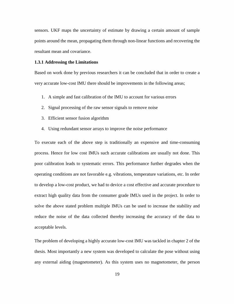
1.3.1 Addressing the Limitations
Based on work done by previous researchers it can be concluded that in order to create a
very accurate low-cost IMU there should be improvements in the following areas;
1. A simple and fast calibration of the IMU to account for various errors
2. Signal processing of the raw sensor signals to remove noise
3. Efficient sensor fusion algorithm
4. Using redundant sensor arrays to improve the noise performance
To execute each of the above step is traditionally an expensive and time-consuming
process. Hence for low cost IMUs such accurate calibrations are usually not done. This
poor calibration leads to systematic errors. This performance further degrades when the
operating conditions are not favorable e.g. vibrations, temperature variations, etc. In order
to develop a low-cost product, we had to device a cost effective and accurate procedure to
extract high quality data from the consumer grade IMUs used in the project. In order to
solve the above stated problem multiple IMUs can be used to increase the stability and
reduce the noise of the data collected thereby increasing the accuracy of the data to
acceptable levels.
The problem of developing a highly accurate low-cost IMU was tackled in chapter 2 of the
thesis. Most importantly a new system was developed to calculate the pose without using
any external aiding (magnetometer). As this system uses no magnetometer, the person

20
wearing the tracking system need not be concerned with interference from ferromagnetic
material present in his vicinity. Also the system is not afflicted by the problem of occlusion
in camera tracking systems.
1.4 Objectives and Methodology
The aim is to build an improved low-cost MEMS IMU which could then be used to build
a cost-effective human motion capture system. In accordance to this objective the following
steps were taken to build yIMU:
1. Accurate error modelling of low-cost IMU and simple calibration to reduce the
accumulative errors.
2. Apply appropriate signal processing techniques to further improve the precision.
3. Implementation of a simple sensor fusion algorithm for orientation tracking.
4. Design of compact hardware.
5. Assess the performance of yIMU.
6. Prepare a kinematic model of human limb for joint angle tracking
7. Assess the system performance
1.5 Outline
The organization and overview for the remainder of the thesis:
Chapter 2 (Development of Low-Cost Inertial Measurement Unit: yIMU) discusses
the design and building of a novel low-cost IMU. Firstly, the error model used to
characterize the behavior of IMU is described followed by using a simplified model
for building yIMU. Following this, the calibration techniques have been described.
Next, we delve into the development of the attitude tracking algorithm to calculate

21
the orientation in 3D space. Details of the process of fabrication of the IMU
hardware is then discussed. Finally, the performance evaluation of the IMU is done
with special consideration to testing the validity of using an opposed configuration
system. The tremendous improvement to yaw stability is then proved.
Chapter 3 (Joint Angle Tracking using Inertial Sensors) is devoted to describing the
process of developing a simple joint angle tracking algorithm. Kinematical
modelling of human upper limb segment is discussed- this involves the assignment
of sensor frames of reference, generation of DH parameters and computation of
transformation matrix. Then we mention the process of sensor-segment orientation
for aligning the body axis frame of the sensor to respective human segment frame.
This is followed by an experiment to test the accuracy of the system.
Chapter 4 (Conclusion) gives a succinct description of the results obtained and
proposes the subsequent inferences pointing to the contribution of this thesis. It also
discusses the future scope of the work and the suggestions for improvements.

22
Chapter 2
DEVELOPMENT OF LOW-COST INERTIAL MEASUREMENT UNIT: yIMU
In this chapter we discuss the development of a low-cost IMU built on Arduino platform.
As a precursor to building an accurate motion tracking system, there was a need to have a
highly precise low-cost IMU. This is the first step to bring such inexpensive inertial sensors
closer to tactical grade performance which would lead wider applications.
In order to achieve better performance, a dual IMU system was chosen that would lead to
better noise performance of the overall system. Experiments were done to validate this
argument. An effective error model for the sensor was built along with an efficient
compensation scheme to remove stochastic and deterministic errors from the sensor
measurements. This was followed by a simple calibration scheme based on the proposed
error model. We also performed a range of detailed tests to understand the nature of sensor
signals. Once the drift and noise from the raw sensor readings were eliminated a quaternion
based complementary filtering scheme was implemented. The choice of a complementary
filter was done to reduce the computational burden on IMU and to increase the battery-life.
Later, the hardware design of yIMU was finalized followed by experiments to evaluate the
performance of yIMU.
Based on this it can be surmised that a novel IMU has built that can be effectively used for
human motion tracking applications.
2.1 Error Modelling and Calibration
Low-cost mems IMUs are not precisely calibrated, hence are affected by various error
sources. This leads to non-accurate scaling, sensor axis misalignments, cross-axis

23
sensitivities and non-zero biases. In order to increase the accuracy, they need to be
calibrated. Identifying the sources of errors afflicting the system is known as error-
modelling and is the first step in the direction of calibrating the IMU. Nevertheless, it has
to be acknowledged that in order for the system to run on Arduino an elaborate error
correction scheme cannot be realistically implemented. Hence a simplified error model has
been built.
In order to minimize the measurement errors in inertial sensors, we need to mathematically
model errors, according to the sources of these errors. Once this is done, we can compensate
for the errors in the measurement equations. In general, these errors can be divided into
two broad categories: deterministic and stochastic (Unsal and Demirbas 2012). Calibration
is defined as the process of comparing instrument outputs with known reference
information. Consequently, the coefficients are determined that force the output to agree
with the reference information for any range of output values (Aggarwal, Syed et al. 2006).
As mentioned before, calibration of the IMUs is of paramount importance to reduce the
deleterious effects of sensor drifts and noises. Hence, a simple calibration scheme has been
followed to meet this requirement. For more in depth treatment of inertial sensor principles
refer (Woodman 2007).
It is important to have a rigorous understanding of the nature of signal to effectively model
it. In section 2.1.4-2.1.7 we do this by performing a slew of tests. Allan variance analysis
and Power Spectrum Density Analysis is done to confirm the “color” of the constituent
signals of inertial sensor. This is important as the probabilistic model we chose to depict
the stochastic error of the sensors depends on it. Next to confirm the Gaussian nature of

24
the signal we perform a Probability Density Function analysis. Usually when modelling
sensor errors it is assumed that the noise predominantly White Gaussian of nature, but to
be sure of whether this hold true and to what extent for MPU6050, these tests need to be
done. This would provide rigor to the discussion in section 2.2.2. Finally, we also perform
drifting bias analysis. This is seldom done as good sensors display this effect over an
extended period of time, for short interval usage (like 10 minutes) this seems to be an
overkill. But if we were to be able to apply yIMU for long-term navigation applications,
this might prove to be useful. These tests provide the groundwork for development of future
more complex sensor fusion algorithms based on the present system.
2.1.1 Types of Errors
Deterministic errors are the kind of errors that can be easily modelled as either they remain
constant and their variations can be simplistically modelling. The quantification of these
errors does not change with time regardless of the state of the system. These errors are
highly temperature dependent hence for advanced calibration usually a lookup table is
generated via laborious experimentation and accordingly compensated in the equations
(Barrett, Gennert et al. 2012). Deterministic errors can be categorized as follows:
1. STATIC BIASES
This is an offset bias that can be noticed at the beginning of collecting raw data
from the IMUs. This is a constant error independent of measurements taken. A
constant bias when integrated causes angular error to grow linearly with time. The
same integration if done twice on accelerometer data to get distance leads to large

25
quadratic errors. These can be corrected by averaging the measurements and
subtracting the offset from the initial measurements.
Ө(𝒕) = 𝒄. 𝒕 (2.1)
where Ө is the integrated angle, c is the error that that grows linearly with time t.
Figure 2.1: Static bias error (Groves 2013)
2. SCALE FACTOR AND MISALIGNMENT ERRORS
Scale factor errors are multiplicative errors that lead to changing the slope of the
sensor measurements. It is to be noted that there is a non-linear term in the scale
factor too but it is usually modelled into once parameter for simplicity.
26
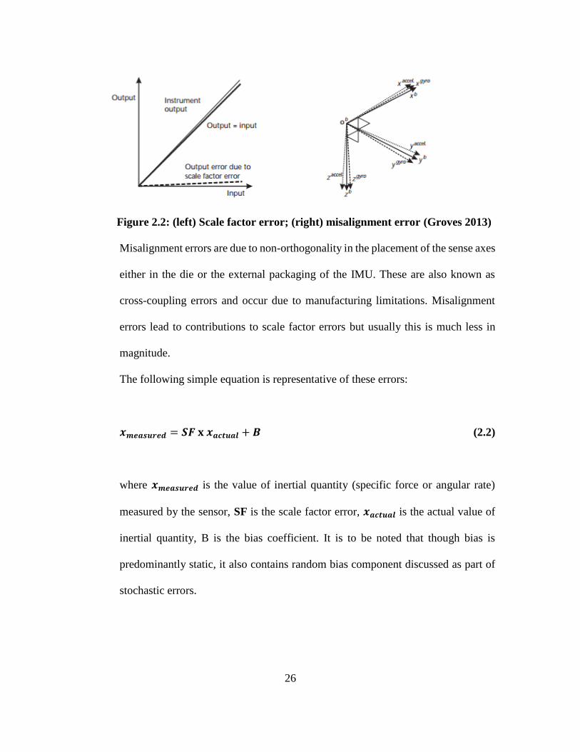
Figure 2.2: (left) Scale factor error; (right) misalignment error (Groves 2013)
Misalignment errors are due to non-orthogonality in the placement of the sense axes
either in the die or the external packaging of the IMU. These are also known as
cross-coupling errors and occur due to manufacturing limitations. Misalignment
errors lead to contributions to scale factor errors but usually this is much less in
magnitude.
The following simple equation is representative of these errors:
𝒙𝒎𝒆𝒂𝒔𝒖𝒓𝒆𝒅 = 𝑺𝑭 𝐱 𝒙𝒂𝒄𝒕𝒖𝒂𝒍 + 𝑩 (2.2)
where 𝒙𝒎𝒆𝒂𝒔𝒖𝒓𝒆𝒅 is the value of inertial quantity (specific force or angular rate)
measured by the sensor, SF is the scale factor error, 𝒙𝒂𝒄𝒕𝒖𝒂𝒍 is the actual value of
inertial quantity, B is the bias coefficient. It is to be noted that though bias is
predominantly static, it also contains random bias component discussed as part of
stochastic errors.

27
Stochastic errors have their source in random processes. This means that these errors
cannot be modelled deterministically and we have to use a probabilistic model as these
errors are non-repeatable and unpredictable meaning there may not be any direct
relationship between input and output. White noise can be removed only by sacrificing the
bandwidth of the sensor as it cannot be removed by calibration. The complexity of
probabilistic model depends on the system on which it is to be implemented. The following
are the different kinds of stochastic errors:
1. MEASUREMENT NOISE
This a zero-mean random process that creeps into the measured sensor data. Usually
modelled as the average error that is the result of high frequency white noise. The
source of this errors cannot be pin pointed and are believed to be inherent to the
nature of MEMS functioning and purported to be thermomechanical in origin.
This can be calculated by using Allan variance analysis (see section 2.2.4). There
we can find that the noise can be modelled as a white noise sequence with zero-
mean uncorrelated variables identically distributed having a finite variance σ2. The
following equation explains the effect of zero-mean random walk error into the
integrated signal.
𝝈Ө = 𝝈√𝜹𝒕. 𝒕 (2.3)
where 𝝈Ө is the standard deviation of the integrated signal that grows proportional
to square root of time. Why is sensor measurement noise modelled as Gaussian

28
white noise? Because white noise has a power spectrum that is flat or equal valued
at all noise frequencies, this can be seen in AV chart. Though we can assume for
the sake of simplicity that measurement noise is white and model it anyway, for the
sake of accuracy it is good to confirm how accurate our model will be by
performing AV or PSD analysis (see sections 2.2.4 and 2.2.5). Similarly, in order
to confirm the Gaussian nature of the sensor signal PDF analysis (see section 2.2.6)
needs to done. This is important because then we can be sure of accuracy when we
use White Gaussian Noise to depict sensor stochastic errors.
2. TURN-ON TO TURN-ON BIAS VARATION
This is the variation in the static bias of the sensor due to transition in power cycle
i.e. as the device is switch on/off the static bias values vary unpredictably. This is
a dynamic bias component and usually measures 10% of static bias (Groves 2013).
As the value if very small we have not given consideration in our simple model
discussed in section 1.2.8.
3. DRIFTING BIAS
This is also known as the random walk error. This is the random drift in the
measured sensor values over time due to change is bias drift values. Usually a first-
order Markov process is used to model the random component of the drift bias. This
effect of this errors accrues over time and is not immediately felt for short durations.
For highly dynamic movements though this has to be taken into consideration and
modelled accordingly.
The nature of these errors have been discussed in more detail in sections 2.2.4-2.2.7, where
we also discuss strategies to quantify or correct them in our sensor fusion design.

29
2.1.2 Temperature Compensation
The actual value of bias and scale factor obtained via calibration differ from operational
value due to difference in temperatures. Hence an accurate thermal model is required. The
importance of this cannot be understated as It is shown that the thermal variation of
accelerometer bias may reach about 0.94 m/s2 for ADI MEMS sensors and gyroscope drift
can reach 50 /sec, over the temperature range from -250 C to 700 C (Aggarwal, Syed et al.
2006). Hence if these thermal variations are not corrected or compensated, it can lead to
very large orientation errors.
For our case we used the ramp method (Shiau, Huang et al. 2012). First the IMUs are placed
flat in the thermal chamber at room temperature. The chamber temperature is controlled to
increase from room temperature to 650 C at approximately 10 C/min. At the same rate
temperature is decreased to -100 C and then heated to room temperature. This cycle is
repeated once more. The advantage of using this against the soak method usually used:
1. The total time of data collection is reduced as we do not wait for sensor
temperatures to stabilize ate each point.
2. The amount of data points collected is increased for every point. 4 sets for each
point as the same temperature is visited twice when heating and cooling.
3. The dynamic variation is mapped as there is continuous change in temperature.
The data is divided in temperature range sets: set1: 00 C to 200 C; set 2: 200 C to 400 C; 400
C to 600 C. Then the raw data is processed using MATLAB and a third degree polynomial
fit drawn.

30
𝑻 = 𝑪𝟏𝒕𝟑 + 𝑪𝟐𝒕𝟐 + 𝑪𝟑𝒕 + 𝑪𝟒 (2.4)
Where T is the compensated parameter, t is the initial uncompensated parameter and Ci is
the coefficient where i= (1 to 4). The real-time data is collected using Megunolink Pro data
acquisition software for Arduino. Figure 2.3 shows the effect of temperature compensation
on gyroscope drift. The IMU is kept still for 2 minutes till the sensor temperature is stable.
Then data is logged for 5 minutes. This is followed by heating the sensors till 550 C using
a heat gun. For this experiment, the IMU was temperature compensated only for the range
200 C to 400 C and 400 C to 500 C. The gyro drift till room temperature of 230 C was close
to zero. Between 230 C to 400 C the drift was around 30 for all the axes. Then the drift
increases to 80 for Y axis and 4.50 for X and Z axes. by the end of 500 C. After that the drift
increases uncontrollably for all axes with Y axes drifting as much as 200 at the end of the
experiment.
It is important to note that in order to more accurately prepare a model for temperature
effects on inertial sensors laborious tests need to be done cycled over weeks to confirm the
repeatability of the compensation algorithm. Also in order to have highly precise model
advanced algorithms need to be implemented that can involve Kalman filters, machine
learning, neural network or even a combination of these. Implementation of these is beyond
the scope of this thesis.

31
Figure 2.3: Temperature Compensation: Legend- gx (red), gy (blue), gz (green),
temp1 (black), temp2 (magenta). (above) The plot for the whole duration; (below) The
blown up version to show temperature compensation effect.

32
2.1.3 Static Bias Compensation
Static bias correction is much simpler than correcting other errors. A least squares
technique (Hamdi, Mohammed I. Awad et al. 2014) was used to arrive at approximate
values of offset bias for each of the axes of both gyroscope and accelerometer. The values
are then stored internally in yIMU and subtracted from the raw reading to get stable
readings. It is very important to remove bias from each axes individually before fusing
them to ensure better correlation.
But we can notice that in the following figures there are improvements in the bias offset by
virtue of combining opposed IMUs. Megunolink Pro was used to acquire data in real time
for these experiments. See section 2.5.1 for evaluation of this effect.

33
Figure 2.4: The bias compensated angular yaw rate for the IMUs (Z axis): Pink is the
combined yaw rate from IMU1 (red) and IMU2 (green)
Figure 2.5: The bias compensated angular roll rate for the IMUs (X axis): Pink (not
clearly visible) is the combined roll rate from IMU1 (black) and IMU2 (indigo)

34
Figure 2.6: The bias compensated accelerometer readings for the IMUs (X axis):
Indigo is the combined roll rate from IMU1 (grey) and IMU2 (pink)
2.1.4 Allan Variance Analysis
Allan Variance is technique to analyze dataset in time domain. Using this we can find out
the noise in the system measurements as a function of time averaging i.e. it expresses the
signal variance as a function of time window over which the signal is averaged. The results
have been presented in section 2.5.2. In this section we describe the process.
For this we initially do a static test of the IMU for a long period of time. Usually up to 12
hours, but in our case due to equipment limitations, the test was done for 8 hours. It was
deemed long enough for us to get a fair estimate of the required readings. For detailed
analysis of drifting bias, longer duration of testing is necessary. The IMU is placed flat in

35
thermal chamber at 270 C. As the IMU is level and still, the only forces acting on it is due
to earth rotation. And the only sources of errors are: drifting bias, measurement noise, static
bias and misalignment errors. Before taking the readings though, it is necessary for the
internal temperature of the IMU to stabilize, so the initial 10 minutes of the readings
collected were ignored.
The static bias and misalignment errors can be removed by averaging the data and
subtracting the offset. Hence we can see that the remainder of the errors in the readings
have measurement noise and drifting bias as their source. Then Allan deviation plots for
this data is calculated for further analysis, for more information of Allan variance method
refer appendix A. What we are specifically looking for in this is the nature of measurement
noise i.e. the color of measurement noise. Allan deviation function is unique to specific
noise color i.e. the slope of the curve depends on the color of the noise: for white noise its
- 1
2 ; random walk noise is +
1
2 ; and for pink noise its zero.
Figure 2.7: Sample Allan Deviation plot for an accelerometer
From the figure 2.7 we can note that the curves first decrease, flatten out then increase. In
order to look for the effects of measurement noise we have to look at the first half of the

36
Allan deviation plot where the effect of measurement noise is predominant. This is because
random walk noise accrues slowly hence initially the percentage of measurement noise in
stochastic noise is much more than drifting bias. As the color of the noise and Allan
deviation function are related we notice this effect on the slope of the curves. For results
of this experiment see section 2.5.2. We can hence say that the measurement noise for
yIMU can in fact be modelled as white noise.
2.1.5 Power Spectral Density Analysis
PSD analysis is used here to confirm the results from Allan variance analysis- we use it to
identify the color of measurement noise in the sensor readings. We can determine the power
of a signal at specific frequencies using this equation:
𝑺(𝒇) = 𝑭(𝑹(г)) (2.5)
where S(f) is the PSD calculated by taking the Fourier transform of R(г), the
autocorrelation function of the signal. We use AlaVar 5.2 to plot the PSD of inertial
sensors.
Figure 2.8: PSD for a sample accelerometer

37
We know that white noise has a power spectrum that is the same at all frequencies, hence
this will show up as flat curve in the plot. Similarly, there are such correlations with other
types of noise, but we will focus on the extent of noise that is white. This is discussed in
detail in section 2.5.3. Based on this result we have confirmed the conclusion of Allan
Variance analysis that the sensor noise is indeed white for yIMU.
2.1.6 Probability Density Function
Probability Density Function (PDF) is used to study the distribution of stochastic noise
(predominantly measurement noise of inertial sensors) of a system. There are many
different kinds of PDFs that might describe a distribution accurately, but the most useful
of them all is Gaussian (normal) distribution represented by the following equation:
𝒇(𝒙) =𝟏
√𝟐𝜫𝝈𝟐𝒆
−(𝒙−ϻ)𝟐
𝟐𝝈𝟐 (2.6)
where ϻ is the mean and 𝝈𝟐 is variance of distribution x.
Figure 2.9: Visual representation of Gaussian distribution
The following are the reasons normal distribution is usually used:

38
1. Most of the systems can indeed be accurately represented by Gaussian PDFs. Hence
in most of the cases IMU errors are also modelled using it.
2. Simple to implement as they have only two parameters:
o ϻ is the sample mean
o 𝝈𝟐 is sample variance
3. By nature of Gaussian distribution, simple manipulations (like adding, subtracting,
etc) also result in a Gaussian distribution. Hence ease of calculations.
But it is important to note that not all low-cost sensors have characteristics consistent
enough to be modelled using Gaussian PDFs. Hence, in the interest of curiosity this test
was done to confirm the premise that the nature of measurement noise is not changed by
using combining two sensors. In section 2.5.4 we will discuss the results in detail.
Nevertheless, the conclusion is that we can use Gaussian distribution to model the
probability distribution of the measurement noises of yIMU. Hence the use of White
Gaussian Noise (WGN) for modelling measurement noise of yIMU has been validated.
2.1.7 Drifting Bias Analysis
As stated previously drifting bias is the bias component that is random in nature and cannot
be precisely modelled deterministically. Due to this we notice the random variations in raw
sensor readings hence the name- ‘random walk’. We approach this problem with a series
of questions:

39
Figure 2.10: Random walk for a sample MPU6050 gyroscope
How to spot drifting bias in Allan variance plot?
The purpose of Allan variance analysis is to visually map the behavior of stochastic errors.
Drifting bias slowly accrues over time, hence larger the time span of raw data collect, larger
will be the noticeable effect of drifting bias. We can see in the Allan deviation plots that
later in the plot, the Allan deviation function curves up gradually (slope +1/2), this is due
to increase in the error contribution due to drifting bias compared to measurement noise.
This shows up towards the end due to the slow moving nature of drifting biases. In fact,
this is the reason we are required to have the raw data collected over large span of time.
How is drifting bias modelled?
In order to model the random walk behavior usually a first-order Markov process model is
used (Barrett, Gennert et al. 2012) with the following equation:

40
𝒃𝒅(𝒊) = 𝝋𝒃𝒅(𝒊 − 𝟏) + 𝜺(𝒊) (2.7)
where 𝒃𝒅 is the drifting bias at time i, φ is the scale factor, and 𝜺 is a zero-mean white
Gaussian white noise process with unknown variance σ2bd.
The reason for using Markov Model is:
o This model is simple with only two parameters- φ scale factor and σ2bd noise
variance. Hence using these parameters in stochastic algorithms does not
unnecessarily increase the complexity of the covariance matrix.
o Easy to implement into a state-space model and can satisfactorily represent highly
dynamic systems.
The Markov process is a stationary process that has an exponential Autocorrelation
Function (ACF). The ACF of a zero-mean first-order Markov process is defined by a
decaying exponential form. As φ represents the amount of correlation that exists between
any two data points in a drifting bias iteration, we can use ACF to obtain value of φ. Hence
we calculate the ACG of the drifting bias data setting lag to 1 for a time step. The drifting
bias data is obtained by removing the measurement noise component from the raw sensor
data, this is done by implementing a moving average filter to the raw data.
Noise variance can be calculated by using the equation:
𝒗𝒂𝒓(𝒃𝒅) =𝛔𝒃𝒅
𝟐
𝟏− 𝛗𝟐 (2.8)
Does using dual IMU system lead to any reduction in drifting bias?

41
Yes, it does. See discussion in 2.7.7 for more information. But we notice that the overall
effect of drifting bias is rather small to impact for small duration of usage, hence we need
not include a special parameter for this in the simplified error model discussed in next
section. In fact, the reduction due to using two IMUs in opposing configuration is small
enough to deem this negligible for motion tracking purposes.
2.1.8 Simplified Error Model
Error modelling is the process of creating a mathematical model of the error sources of a
sensor measurement in order to improve the measured physical quantity. The complexity
of the error model depends on the application and the processing power available. Also
analysis discussed in sections 2.2.4- 2.2.7 demonstrate the validity of using WGN model
for stochastic errors and the drifting bias mitigation effect in yIMU. Keeping this in mind,
following is the simplified error model that has been used in orientation estimation of
yIMU:
𝒂𝒎 = 𝒂 + 𝒃𝒂 + 𝒏𝒂 (2.9)
Where am is the measured value of acceleration (raw readings), a is the actual value of the
measured inertial quantity (specific force), ba is the static bias of the accelerometer, and na
is the accelerometer noise. Similarly, we have,
𝒈𝒎 = 𝒈 + 𝒃𝒈 + 𝒏𝒈 (2.10)
Where am is the measured value of gyroscope (raw readings), g is the actual value of inertial
quantity (angular rate), bg is the static bias of the accelerometer, and ng is the gyroscope
noise.

42
The static biases have been compensated as discussed in section 2.2.3. We have not
compensated for scale factor/ misalignment errors in the equation as we did not have the
equipment (precision rate table) to carry out the technique with enough accuracy to justify
any real improvements in measurements. Temperature compensation was done as shown
in section 2.2.2.
The noise part is interesting; we have relied on two techniques to compensate for it:
1. Common Mode Effect (CME)
2. Threshold filter
The details of using CME is discussed in section 2.2.2. According to our knowledge no
other research group has used MPU6050 low-cost IMUs to successfully apply CME. This
takes care of the stochastic errors (measurement noise, drifting bias and, environmental
effects due to temperature and vibration) to a large extent as discussed in section 2.5. In
addition, we have used a threshold filter to further remove the remaining noise components.
The details of this have been discussed in section 2.3.
43
2.2 Dual IMU System
Using redundant sensor array is imperative to increase the performance of a low-cost IMU
system if ever it has to rise to the level of tactical grade sensors. Inertial sensors arranged
in pre-determined geometry to measure inertial quantities to exploit the design
characteristic of the sensors such that the errors exhibited are smaller than those obtained
by simple averaging (Yuksel 2011). For application to human motion tracking where the
compactness and simplicity has to be taken into account, the use of a dual IMU system is
justified instead of using large sensor arrays by exploiting the concept of common mode
effect (Martin, Groves et al. 2013). The premise was that if the 3-axis sensors were arranged
so their sensitive axes were facing in opposite directions when the output was combined
the errors due to temperature and vibration (environmental effects) could be reduced.
2.2.1 Redundant IMUs
A single IMU is used to calculate inertial quantities. In order to seek better navigation
solutions more than one IMU could be used to calculate the same inertial quantities but
with greater performance- such system of sensor arrays are called as redundant IMUs. The
information collected from these multiple sensors is processed to generate a virtual IMU.
A detailed survey of the state of array techniques could be found in (Nilsson and Skog
2016). The exact technique used to generate this virtual IMU differs based on complexity
of the system. An example of an INS + GPS fusion is given in figure 2.11.

44
Figure 2.11: A virtual IMU observation fusion architecture (Bancroft and Lachapelle
2011)
Depending on the type of sensors, number of sensors, sensor fusion technique employed
and application constraints redundant arrays have the following advantages:
1. The noise performance of the combined output is better due to averaging of
stochastic errors. This leads to increase in the measurement accuracy of inertial
quantities.
2. The dynamic measurement range could be extended beyond that of individual
sensors by utilizing the spatial separation between the sensors (Skog, Nilsson
et al. 2016).
3. Robust fault tolerance algorithms could be deployed for better redundancy in
risky situations by including the redundant measurements in the covariance of
the measurement errors so as to determine the reliability of the measurements.
Not just faults in the system could be detected but also isolated to prevent
propagation of those faults in the navigation equations (Groves 2013).

45
4. Geometrical constraints play a major role in assessing the quality of
measurement with various skew-redundant techniques developed for advanced
applications (Yuksel 2011).
2.2.2 Common Mode Effect
If the family of sensors is guaranteed to have similar external factor dependence
characteristics, then these sensors can be formed into an array to be used to suppress those
effects. A correlation between IMUs is shown by Yuksel et al (Yuksel, El-Sheimy et al.
2010) that reduce the temperature effect gyroscope bias which if applicable to MP6050
could be useful. This has been attested for MPU6050 as shown in section 2.6. This further
reduces the computational complexity of the sensor fusion algorithm used in the low cost
IMU.
Figure 2.12: Dual axes configuration { based on (Yuksel, El-Sheimy et al. 2010) }
Theoretically this technique could work for correlated even order errors (Martin, Groves
et al. 2013) e.g. If the static bias of a sensor is estimated to be positive always then

46
combining the data from two opposing axes could effectively reduce the error more so than
just averaging them. Figure 2.12 shows the combined raw data for two IMUs in such a
configuration. We can notice a huge improvement without using any extra computation
complexity. This is the key to building an efficient orientation tracker. The important point
here is that the sensor physical properties of in-plane and out-of- plane sensors should not
vary. As no information about this could in the datasheet we contacted Invensense (the
manufacturers) to check this. It was reported that there are no such variations due to
manufacturing process.
From the results in section 2.5 we can see that we have in fact successfully applied this
technique to MPU6050 IMUs. But how could we justify the cost of adding one extra sensor
in the name of performance improvement? This is because calibration of MEMS IMUs is
an expensive affair increasing the per unit cost of an IMU to hundreds of dollars (Martin,
Groves et al. 2013).

47
Figure 2.13: Gyroscope output (in LSB) comparison for two IMUs with opposed sense
axes: std of gyroX1 is 12.9 LSB; gyroX2 is 13.84 LSB and combined is 9.417.
Figure 2.14: Gyroscope drift from two IMUs with opposed sense axes

48
2.3 Sensor Fusion
Sensor fusion is a process by which data from several different sensors are "fused" to
compute something more than could be determined by any one sensor alone. For our
application it means we need to fuse data from multiple inertial sensors to help us determine
the orientation in 3D space. We use a quaternion based complementary filter scheme to
achieve this end. The reason for using quaternions is to avoid the use of additional function
in the code to deal with Euler angles and to avoid gimbal lock. Also complementary filter
is not computationally expensive compared to stochastic algorithms like Kalman Filter.
Though it must be admitted that with a more intricately crafted sensor fusion scheme the
attitude estimation performance of the system could be greatly improved (Paina, Gaydou
et al. 2011) by virtue of improved bias estimation.
2.3.1 Representing Angles
Depiction of orientation of a rigid body can be done in various forms: axis-angle, Euler
angles, quaternions, etc. In this section we explore the problem of mathematically
representing the orientation of a rigid body using inertial sensors.
EULER ANGLES
Euler angles are the most widely used representation technique which is both simple to use
and intuitive to understand. The foundation of this technique is the premise that any
orientation can be dissected and represented as a combination of three rotations about the
orthogonal body reference frame of the object. These three rotations though have to vector
added in a particular order for universal order as angular rotations are not commutative.

49
Figure 2.15: Euler angle representation (CH_Robotics)
There are two problems with using Euler angle representation:
1. Computationally expensive: Calculation of trigonometric functions in embedded
processors takes a longer amount time than simple floating point math.
2. Gimbal Lock: This is the phenomena when the orientation of a body cannot be
unique determined using a particular sequence of Euler Angles. This happens
usually when the pitch appears 900 as can be seen when we substitute Ө in equation
2. with 900.
MEASURING ATITTUDE USING ACCELEROMETERS
The measured specific force of accelerometer a can be represented in vector form as
follows:
𝒂𝒃̅̅ ̅ = 𝜴𝒃̅̅ ̅̅ 𝑿 𝑽𝒃̅̅̅̅ − 𝒈𝒃̅̅̅̅ = 𝜴𝒃 ̅̅ ̅̅ 𝑿 𝑽𝒃̅̅̅̅ − 𝒈 [−𝒔𝒊𝒏Ө
𝒔𝒊𝒏𝝋 𝒄𝒐𝒔Ө𝒄𝒐𝒔𝝋 𝒔𝒊𝒏Ө
] (2.11)

50
where φ and Ө represent roll and pitch respectively; b superscript represents the body
frame; V represents translational acceleration; 𝜴 X V represents angular acceleration; and
g is gravity. If the body is at rest V=0 and if rotational acceleration is neglected, we have:
𝒂𝒃̅̅ ̅ = −𝒈 [−𝒔𝒊𝒏Ө
𝒔𝒊𝒏𝝋 𝒄𝒐𝒔Ө𝒄𝒐𝒔𝝋 𝒔𝒊𝒏Ө
] (2.12)
On further calculations (Pedley 2013) we arrive at:
𝒕𝒂𝒏𝝋 = 𝒂𝒕𝒂𝒏𝟐(𝒂𝒚𝒃, 𝒂𝒛
𝒃) (2.13)
𝒕𝒂𝒏Ө = 𝒂𝒕𝒂𝒏𝟐(−𝒂𝒙𝒃, √𝒂𝒚
𝟐 + 𝒂𝒛𝟐) (2.14)
From equation 2.13 we get the roll and equation 2.14 we get the yaw.
Figure 2.16: Measuring tilt using accelerometers (Innoventions)
MEASURING ATTITUDE USING GYROSCOPES
The measured angular rate 𝜴 in vector form can be represented as:
𝜴 = [𝒑𝒒𝒓
] (2.15)
51
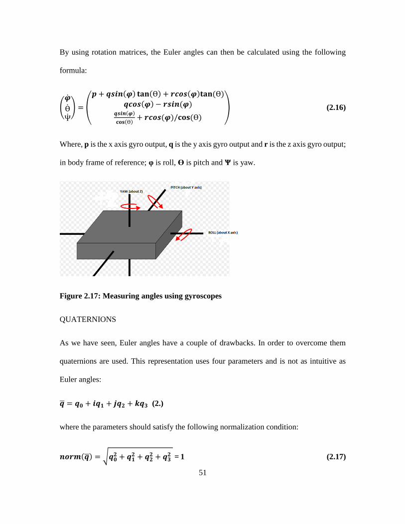
By using rotation matrices, the Euler angles can then be calculated using the following
formula:
(�̇�
Ө̇Ѱ̇
) = (
𝒑 + 𝒒𝒔𝒊𝒏(𝝋) 𝐭𝐚𝐧(Ө) + 𝒓𝒄𝒐𝒔(𝝋)𝐭𝐚𝐧 (Ө)
𝒒𝒄𝒐𝒔(𝝋) − 𝒓𝒔𝒊𝒏(𝝋)𝒒𝒔𝒊𝒏(𝝋)
𝐜𝐨𝐬(Ө)+ 𝒓𝒄𝒐𝒔(𝝋)/𝐜𝐨𝐬 (Ө)
) (2.16)
Where, p is the x axis gyro output, q is the y axis gyro output and r is the z axis gyro output;
in body frame of reference; φ is roll, Ө is pitch and Ѱ is yaw.
Figure 2.17: Measuring angles using gyroscopes
QUATERNIONS
As we have seen, Euler angles have a couple of drawbacks. In order to overcome them
quaternions are used. This representation uses four parameters and is not as intuitive as
Euler angles:
�̅� = 𝒒𝟎 + 𝒊𝒒𝟏 + 𝒋𝒒𝟐 + 𝒌𝒒𝟑 (2.)
where the parameters should satisfy the following normalization condition:
𝒏𝒐𝒓𝒎(�̅�) = √𝒒𝟎𝟐 + 𝒒𝟏
𝟐 + 𝒒𝟐𝟐 + 𝒒𝟑
𝟐 = 1 (2.17)

52
The representation is for the axis about which rotation takes place and the angle by which
it is rotated. The conversion between Euler angle representation and quaternions can be
written as:
𝒒𝟎 = 𝒄𝒐𝒔Ө
𝟐
𝒒𝟏 = −𝒓𝒙𝒔𝒊𝒏Ө
𝟐
𝒒𝟎 = −𝒓𝒚𝒔𝒊𝒏Ө
𝟐
𝒒𝟎 = −𝒓𝒛𝒔𝒊𝒏Ө
𝟐
where 𝒓𝒙 , 𝒓𝒙 𝑎𝑛𝑑 𝒓𝒙 are the components of the unit vector �̅� in the frame of rotation.
Figure 2.18: Euler to quaternion conversion
The most important operation on quaternions is calculating the product:
𝒒𝑪𝑨̅̅̅̅ = 𝒒𝑪
𝑩̅̅̅̅ ⦻ 𝒒𝑩𝑨̅̅̅̅ (2.18)

53
where 𝒒𝑪𝑨 is the rotation to C with respect to A; 𝒒𝑩
𝑨 is the rotation to B with respect to A;
and 𝒒𝑪𝑩 is the rotation to C with respect to B. Hence we have the following resultant matrix
that uniquely represents the manipulation:
𝒒𝑪𝑨̅̅̅̅ = [
𝒂𝟎 𝒃𝟎 − 𝒂𝟏 𝒃𝟏 − 𝒂𝟐 𝒃𝟐 − 𝒂𝟑 𝒃𝟑
𝒂𝟎 𝒃𝟏 + 𝒂𝟏 𝒃𝟎 + 𝒂𝟐 𝒃𝟑 − 𝒂𝟑 𝒃𝟐
𝒂𝟎 𝒃𝟐 − 𝒂𝟏 𝒃𝟑 + 𝒂𝟐 𝒃𝟎 + 𝒂𝟑 𝒃𝟏
𝒂𝟎 𝒃𝟑 + 𝒂𝟏 𝒃𝟐 − 𝒂𝟐 𝒃𝟏 + 𝒂𝟑 𝒃𝟎
] (2.19)
where 𝒒𝑪𝑩̅̅̅̅ = [𝒂𝟎 𝒂𝟏 𝒂𝟐 𝒂𝟑 ] and 𝒒𝑪
𝑨̅̅̅̅ = [𝒃𝟎 𝒃𝟏 𝒃𝟐 𝒃𝟑 ] are the respective quaternions.
2.3.2 Complementary Filter
There are many sensor fusion algorithms that give good attitude estimation. Extended
Kalman Filter is most commonly used stochastic estimator. But to give accurate estimated
the modelling of measurement and update matrices is very important. This leads to
increased complexity which might not be required for some applications. Notwithstanding
this, EKF is still the standard algorithm used for inertial navigation purposes (Quoc, Sun
et al. 2015). Hence the use of complementary filters makes more sense in such situations.
Complementary filters can be used with a group of sensors having complementary signal
characteristics. Accelerometers are susceptible to high frequency noise and gyroscopes are
susceptible to low frequency noise, hence complementary filter can be used to
appropriately blend both the sensor attitude (figure 2.19) updates to arrive at a superior
reading without the use of a stochastic estimator algorithm like Kalman filter.

54
Figure 2.19: Complementary filter structure
This figure demonstrates a 1D complementary filter. Mathematically, this can be
represented by the following transfer function:
Ө =𝟏
𝟏+𝑻𝒔𝒂 +
𝑻𝒔
𝟏+𝑻𝒔 𝟏
𝒔𝒈 =
𝒂+𝑻𝒈
𝟏+𝑻𝒔 (2.20)
where Ө is the final fused angle, a is the angle calculated by accelerometer, g is the angular
rate calculated by the gyroscope, and T is the “time-constant”. This leads to fusing low-
frequency estimate from the accelerometer and high frequency estimate from the
gyroscope. The final recursive equation can hence be written as:
Ө𝒊 = 𝜶Ө𝒊−𝟏 + (𝟏 − 𝜶)𝒂𝒊 + 𝜶𝒈𝒊𝒅𝒕 (2.21)
where i is the present time-step, dt is the sampling time, α is the cutoff parameter such that
𝜶 =𝑻
𝑻+𝒅𝒕 more frequently calculated by trial and error.
2.3.3 Sensor Fusion Scheme
The sensor fusion uses complementary filter explained above. But before that the following
steps are taken to ensure accurate data. The filter parameters need to be tweaked according

55
to the sensor under consideration as there is wide variation in performance in low-cost
sensors.
Calibration
In order to have good data calibrating the sensors is very important. In section 2.2, the
methodology and the error model has been explained in detail. It entails, removing the bias
offset first as it is the leading cause of huge errors. It is pretty easy to remove by averaging
when the senor is still.
Centralized data fusion
The raw data from the dual IMU system is fused together to take advantage of the common
mode effect as described previously. The following equations explains the process:
𝑮 =𝑮𝟏−𝑮𝟐
𝟐 (2.22)
where 𝑮𝟏 and 𝑮𝟐 are the values of inertial quantities of sensor 1 and 2 respectively;
𝑮𝒊 = 𝒈𝒊 + 𝒃𝒊 + 𝒏𝒊 (2.23)
Where i=1,2 are for the sensors; g is the actual inertial quantity; b is the bias; and n is the
noise.
On combining data, this is what we get:
𝑮 =𝟏
𝟐(𝒈𝟏 + 𝒃𝟏 + 𝒏𝟏) −
𝟏
𝟐(−𝒈𝟐 − 𝒃𝟐 + 𝒏𝟐) (2.24)
where we note that the inertial quantity measured by the second sensor is negative of the
first sensor i.e. 𝒈𝟏 = 𝒈𝟐 = 𝒈 . The trend in bias is opposite though not the same and the

56
noise part is random in nature, though as we have seen in section 2.2 there is averaging
effect due to this configuration- i.e. the combined noise of the system is 𝒏𝟏+𝒏𝟐
𝟐.
Therefore, finally we have:
𝑮 = 𝒈 + 𝒌𝒃 + 𝒑𝒏 (2.25)
where k and p depend on the values of changing bias and noise but less than 1.
Filtering
The gyro data was band pass filtered to remove high frequency disturbances and the
accelerometer data was low pass filtered to remove high frequency noise.
Gravity Effect
The accelerometer is sensitive to the effect of gravity which makes it difficult to get actual
sensor accelerations along the axis aligned with gravity. In order to take care of it we need
to remove the gravity effect by turning the sensor frame to global frame. This need not be
performed if the application does not allow the sensor to be flipped.
The following equations gives an idea of the process:
𝒂𝑮 = 𝑨𝑮 − [𝟎𝟎
𝟗. 𝟖𝟏] (2.26)
where 𝒂𝑮 is the final acceleration in global frame; 𝑨𝑮 is the transformed acceleration; and
assuming gravity is constant at 9.81m/s2.
𝑨𝑮 is given by the following equation:

57
𝑨𝑮 = 𝑹𝑺𝑮 ∗ 𝑨𝒔 (2.27)
where 𝑨𝒔 is the measured acceleration in sensor frame and 𝑹𝒔𝑮 is the rotation matrix from
sensor to global frame.
Thresholding
Now that the sensor noise has been reduced a lot, we apply a threshold filter to remove any
residual noise from the filtered data. This has the effect of removing any time varying bias/
noise from the readings. This though leads to reduction in the bandwidth of the sensor
giving rise to problem of not detecting very slow motions like 0.5 deg/s. But for most
applications this could be neglected.

58
2.4 Hardware Design
The overarching goal of the hardware design is to have a compact low-cost IMU that can
efficiently run the smart- algorithm. The yIMU consists of two MPU6050 IMUs with in-
built temperature sensor. The design was minimalist keeping in mind that this is not a
production version. The design went through many prototyping cycles. The hardware
characteristics of final prototype is described in Table 2.1. This has a stacked shield layout,
which was used in the development of the calibration procedure and tracking algorithm.
The boards were fabricated in-house at ASU polytechnic electronics lab.
Physical
Characteristics
Dimensions 62x65x42 mm
Weight 107 g with case
Sensor
Specifications
MPU 6050
Accelerometer
Range ±2g
Resolution 3.9mg/LSB
0g Bias Level ±40 mg (X,Y); ±80
mg (Z)
Noise Performance <3.9 mg RMS
Gyroscope
Range ±250 dps
Resolution 0.0696 dps/LSB
0g Bias Level ±40 dps
Noise Performance 0.38 dps RMS
Temperature
Sensor operation
range
-400 C to 800 C
Temp compensation
range
50C to 55 0C
Microcontroller
Specifications
Arduino pro mini
ATmega 328p

59
16 MHz clock
frequency
Connectivity
Bluetooth HC-06 class II with
10 m range
USB FTDI
Power
Specifications
Li-ion battery
800mAh
3.7 V
Table 2.1: Hardware specification of yIMU v1.4
2.4.1 System Design
yIMU v1.4 is the testing version which has two boards stacked on top of each other. The
base board houses the charging circuit and the Arduino pro-mini microcontroller board
along with a power switch. The charging is done via a micro-USB whereas the
programming is done via an FTDI cable. The board is also connected to a Li-ion battery
that powers the entire setup.

60
Figure 2.20: The stacked boards in yIMU v1.4
The top board houses two MPU6050 IMUs with their sense axes in opposing directions.
The x and y axes have been flipped in the algorithm (Figure ) to account for the
impossibility to physically place the corresponding axes opposing each other. As those
axes were manufactured in-plane during fabrication there should be no loss in accuracy.
An HC-06 Bluetooth module is packed aside the sensors as shown for wireless
connectivity.

61
Figure 2.21: Sense axes of the dual IMU system
It is to be noted that the size of the board can be reduced further by increasing the layers in
the board. This is beyond the capabilities of our in-house fabrication facility and also would
increase the cost of the prototype, hence it has not been physically realized though there is
definitely scope for further improvements in the design. We used I2C mode of serial
communication between the sensors and the microcontroller which allows sensor registers
to be read upto a maximum of 400kHz. Though this is much slower than SPI (which could
in theory allow upto 20MHz in communication speed), we would not have to deal with
high frequency signal errors arising from its use and to accommodate for it in our circuit
design.
2.4.2 Enclosure Design
The enclosure was 3D printed using FDM (Fused Deposition Modelling) method in lab.
The major concern with enclosure design was to be able to house all the required circuitry

62
with proper alignment within the housing. Adequate care was taken during the design of
the enclosure to address this issue. Another problem was to ensure that the IMU enclosure
to remains fixed firmly to the body to prevent unnecessary movements. To solve this a
simple Velcro strap with padding was used.
Figure 2.22: Enclosure for yIMU v1.4 with straps

63
2.5 Performance Evaluation
In this section we test to check for improvements in sensor parameters due to yIMU
configuration. We also discuss the experimental results of the implementation of the
algorithm.
2.5.1 Testing Viability of Common Mode Effect
As discussed in section 2.2.1 environmental effects are felt more severely in low cost IMUs
than navigation grade IMUs by virtue of their inherent working principle and nature of
manufacturing process. In this section we note the effect of temperature and vibration on
yIMU systems. It is to be noted that these effects are dependent on the product model of
sensor tested (MPU6050) and do not hold true for all IMUs. The exact values of the effect
changes from sensor to sensor but these results point towards the prevalent trends in the
environmental effects on yIMU.
TEMPERATURE EFFECT
Procedure: The yIMU system is kept flat and stationary, and data is logged for 5 minutes
at room temperature. Then it is heated using a heat gun for 5 mins till around 500 C. Then
it is allowed to cool to room temperature. Raw accelerometer and gyroscope data is
collected for further analysis.

64
Figure 2.23: Heraeus UT12p Thermal Chamber
Results: Figure 2.24 shows the temperature profile followed for the experiment. This
representative temperature is from the sensor at IMU1. Then a linear fit for the scatter plot
data from IMU1, IMU2 and the yIMU system is calculated using MATLAB as depicted in
Figure 2.25. The data for each of the axes is documented in Table 2.2. Compare the
temperature drift trend and extent of effect for each of the axes.
Figure 2.26 compares the angular rate output temporal trend. The pattern is similar for all
the axes.

65
Figure 2.24: Temperature profile of the experiment
Figure 2.25: Sample scatter plot of acc axis X for IMU1: the yellow line is the linear fit
for the data

66
Figure 2.26: Sample scatter plot of gyro axis X for IMU2: the yellow line is the linear
fit for the data
NAME Acc- SLOPE
(LSB/0C)
Acc-
INTERCEPT
(LSB)
Gyro-SLOPE
(LSB/0C)
Gyro-
INTERCPT
(LSB)
IMU1-X 10.906 -734.75 -5.0286 162.08
IMU1-Y -9.1273 696.33 10.55 -360.99
IMU1-Z -7.2778 16847 2.3697 -85.397
IMU2-X -9.2803 -504.68 1.3062 -37.572
IMU2-Y 1.0003 -252.34 -1.4636 +56.49
IMU2-Z 2.8734 16283 -0.44031 +16.915
Table 2.2: The results of linear best fit between sensor output and temperature for
MPU6050 in opposing configuration

67
Figure 2.27: Comparison of temperature effect trends for gyro X of IMU1, IMU2 and
combined output
VIBRATION EFFECT
Procedure: IMU is placed flat z axis up on a surface at rest for a minute, followed by
vibration for 20 s. The setup was vibrated at 60 Hz using a shaker. The raw accelerometer
and gyroscope outputs are recorded after correcting for offset bias. The temperature of the
setup was checked to be constant.

68
Figure 2.28: The FMC shaker used for vibration testing
Results: The following are the results for testing done on yIMUs. A moving average filter
was used to filter the raw data in MATLAB. Some questions to ponder over:
1. What is the effect of vibration on accelerometer and gyroscope?
2. What are the trends for the opposing axes?
We can see the trend from the figure 2.29 which says that opposing sense axes do reduce
the vibration effect. They obviously do not cancel each other out, but the characteristics
are good enough. For yIMU data point to the fact that for MPU6050 this arrangement does
reduce effect of vibration. But dynamic vibration tests need to be done to ascertain its
applicability in highly agile field situations.
Answers:
1. Firstly, looking at the effect on accelerometers of IMU1 we can see in figure 2.29
that there is no significant effect on bias drift after vibration (at 60 Hz). Also there

69
is no pronounced vibration along Z axis. In the case of gyroscopes however, we can
see that the axes perpendicular to the vibration axis show pronounced disturbance
compared to the Z axis gyro. This is to be expected as the proof mass of gyroscope
is designed to measure the angular rate not displacement. The effects are similar for
IMU2
Figure 2.29: Effect of vibration on IMU1 accelerometers
Figure 2.30: Effect of vibration on IMU1 gyroscopes

70
2. We can see from the figures below that for the vibrating axes, opposing axis
obviously have approximately opposing trends during the vibration phase. Hence,
combining their outputs leads to partial vibration cancellation. For the cross axes
though the cancellation is not significant as seen in figure 2.31.
Figure 2.31: Effect of vibration on vibration axis (Z axis): (above) The whole duration;
(below) For the duration of vibration

71
Figure 2.32: Effect of vibration on cross axis (X axis): For the duration of vibration
BIAS ERROR
Bias error refers to deterministic error due to static bias offset here. If this is unaccounted
for it could be the largest source of integration error in inertial navigation. Hence we
compare the bias error of a single IMU to the yIMU to get an idea of improvement in bias
performance. For details of random bias component see section 2.5.5.
Procedure: Mean of around 5 minutes of static data was collected for each of the axes of
IMY-1 and yIMU.
Result: There is noticeable reduction in the bias error in yIMU compared to IMU-1.
IMU-1 Accelerometer
(mg)
yIMU- Accelerometer
(mg)
X 0.2110 0.0998
Y -1.1895 -0.2325
Z 101.4821 1.6910
Table 2.3: Accelerometer bias error

72
IMU-1 Gyroscope
(deg/s)
yIMU- Gyroscope (deg/s)
X 0.0264 0.0196
Y -0.1488 -0.0666
Z 12.6922 6.3358
Table 2.4: Gyro bias error
2.5.2 AV Results
Procedure: The static bias and misalignment errors can be removed by averaging the data
and subtracting the offset. Hence we can see that the remainder of the errors in the readings
have measurement noise and drifting bias as their source. This data can now be analyzed
using Allan variance analysis. We have used MATLAB to generate Allan deviation plots.
Results:
In order to analyze the AV plots we need look at the following four points on the graph:
1. Point A: This is the starting point of the graph that represents standard deviation of
noise for any one single measurement point. This gives us an idea of how noisy a
single measurement can be, it is to be noted that this mentions the probability of
noisy measurements not the certainty of it. For example, if point A measures 0.07
g (for figure 2.34) then 1 standard deviation of the measurements have error of
0.07g in the measurement and rest will have errors greater than that.
2. Slope A: This is the slope for the first part of the AV graph before the dip. This part
is used to analyze the measurement noise, that depends on the influence of high
frequency errors. For example case, in figure 2.34, slope A is -0.483754 that means
it is close to the white noise slope of -0.5, hence we can say that the measurement
errors are predominantly white in color.

73
3. Point B: Represents the bias stability of the sensor. It gives you the lowest possible
value of bias error generated in a sensor. The lower the value, the better sensor it
is. In figure 2.34, the bias stability of accelerometer X axis this particular MPU6050
is 0.0057 g.
4. Slope B: This is the slope for the second part of the AV graph, after the dip. This
part is used to analyze the random walk errors, that depends on the influence of low
frequency errors. We see that the slope B for figure 2.34 is 0.313607, meaning it is
close to random walk slope of +0.5.
ACCELEROMETER PERFORMANCE
Figure 2.34: Allan Deviation plot for IMU-1 accelerometer X

74
Figure 2.35: Allan Deviation plot for yIMU accelerometer X
POINT A
(g) SLOPE A
POINT B
(g) SLOPE
B
IMU-1 X 0.07 -0.483754 0.0057 0.313607
IMU-1 Y 0.07 -0.519263 0.0035 0.149470
IMU-1 Z 0.07 -0.464424 0.00480 0.280849
yIMU X 0.07 -0.490277 0.0026 0.383257
yIMU Y 0.07 -0.495157 0.0018 0.421459
yIMU Z 0.07 -0.485253 0.0025 0.564556
Table 2.5: Comparing the results of AV analysis between IMU-1 and yIMU
accelerometers
GYROSCOPE PERFORMANCE
Figure 2.36: Allan Deviation plot for IMU-1 gyroscope X

75
Figure 2.37: Allan Deviation plot for yIMU gyroscope X
POINT A
(deg/s)
SLOPE A
POINT B
(deg/s)
SLOPE B
IMU-1 X 0.07 -0.51176 0.0053 -0.40475
IMU-1 Y 0.07 -0.522333 0.0042 -0.40306
IMU-1 Z 0.07 -0.527713 0.0026 0.28838
yIMU X 0.07 -0.519355 0.0029 0.484973
yIMU Y 0.07 -0.505054 0.0025 -
yIMU Z 0.07 -0.514046 0.0023 0.476239
Table 2.6: Comparing the results of AV analysis between IMU-1 and yIMU
gyroscopes
The following are the results from the AV plots shown above:
1. The remainder of the AV plots are in appendix B. we note that point A is the same
for both IMU-1 and yIMU. This should be expected as this point negates the effect
of combining data from two IMUs. This shows the noise content of a single
measurement sample; hence the effect of averaging is negated.
2. Comparing the slopes, we see that the measurement noise for yIMU is more close
to -0.5 slope than IMU-1, this means that the white noise modelling of measurement
noise approximates the behavior of yIMU better.
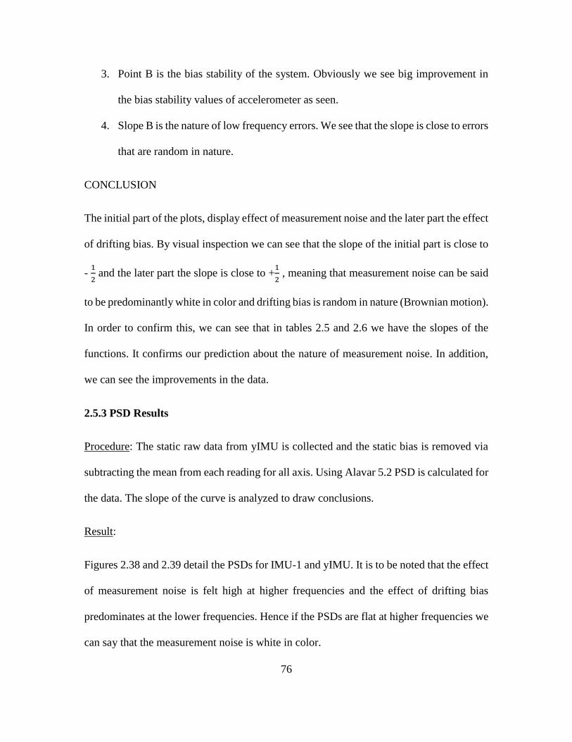
76
3. Point B is the bias stability of the system. Obviously we see big improvement in
the bias stability values of accelerometer as seen.
4. Slope B is the nature of low frequency errors. We see that the slope is close to errors
that are random in nature.
CONCLUSION
The initial part of the plots, display effect of measurement noise and the later part the effect
of drifting bias. By visual inspection we can see that the slope of the initial part is close to
- 1
2 and the later part the slope is close to +
1
2 , meaning that measurement noise can be said
to be predominantly white in color and drifting bias is random in nature (Brownian motion).
In order to confirm this, we can see that in tables 2.5 and 2.6 we have the slopes of the
functions. It confirms our prediction about the nature of measurement noise. In addition,
we can see the improvements in the data.
2.5.3 PSD Results
Procedure: The static raw data from yIMU is collected and the static bias is removed via
subtracting the mean from each reading for all axis. Using Alavar 5.2 PSD is calculated for
the data. The slope of the curve is analyzed to draw conclusions.
Result:
Figures 2.38 and 2.39 detail the PSDs for IMU-1 and yIMU. It is to be noted that the effect
of measurement noise is felt high at higher frequencies and the effect of drifting bias
predominates at the lower frequencies. Hence if the PSDs are flat at higher frequencies we
can say that the measurement noise is white in color.

77
From the figures we can say that for frequencies above 1Hz the PSD is pretty flat, as also
confirmed by calculating the slopes. For figure 2.38 the slope was S(f)=f^(-0.35).
Figure 2.38: PSDs for IMU-1: (above) accelerometer (below) gyroscope for X axis
NAME PSD SLOPE
accX -0.35
accY -0.052
accZ -0.33
gyroX -0.018
gyroY -0.03
gyroZ 0.032
Table 2.7: PSD slope values for IMU-1

78
Figure 2.39: PSDs for yIMU: (above) accelerometer (below) gyroscope for X axis
NAME PSD SLOPE
accX -0.058
accY -0.038
accZ -0.062
gyroX 0.007
gyroY 0.0018
gyroZ -0.012
Table 2.8: PSD slope values for yIMU
2.5.4 PDF Results
Procedure: The static raw data from yIMU is collected and the static bias is removed via
subtracting the mean from each reading for all axis. Using MATLAB the noise data is

79
plotted as histogram to show the number of occurrences per value. Then a normal
distribution over the sample time is also plotted over the same histogram to see the fit.
Result: The confirmation of Gaussian distribution is done visually by noticing the match
between the histograms and the Gaussian curve. From figure 2.40 we can conclude that we
can indeed use Gaussian distribution to model measurement noise of MPU6050. Table 2.9
shows the sample variances of the IMU-1.
Figure 2.40: IMU-1 measurement noise histogram with Gaussian PDF plotted over it
(above) accelerometer X (below) gyroscope X

80
NAME VARIANCE
accX 0.0357
accY 0.0361
accZ 0.0177
gyroX 0.0500
gyroY 0.0625
gyroZ 0.0261
Table 2.9: IMU-1 measurement noise variances
Figure 2.41: yIMU measurement noise histogram with Gaussian PDF plotted over it
(above) accelerometer X (below) gyroscope X

81
NAME VARIANCE
accX 0.0255
accY 0.0136
accZ 0.0118
gyroX 0.0482
gyroY 0.0463
gyroZ 0.0179
Table 2.10: yIMU measurement noise variances
In figure 2.41 we see the histograms for yIMU, we notice that the fit is not affected in any
way hence the assumption of using Gaussian PDFs is validated. We notice a better fit in
yIMU than in IMU-1.
2.5.5 Drifting Bias Analysis Results
Procedure: Once the static bias has been accounted for we perform a simple moving
average on the resulting raw data to nullify the effect of measurement error on the raw data.
The remaining effects are solely due to random walk error. We then calculate the ACF for
this time series to find out Markov parameters as discussed in section 2.2.7.
Results:
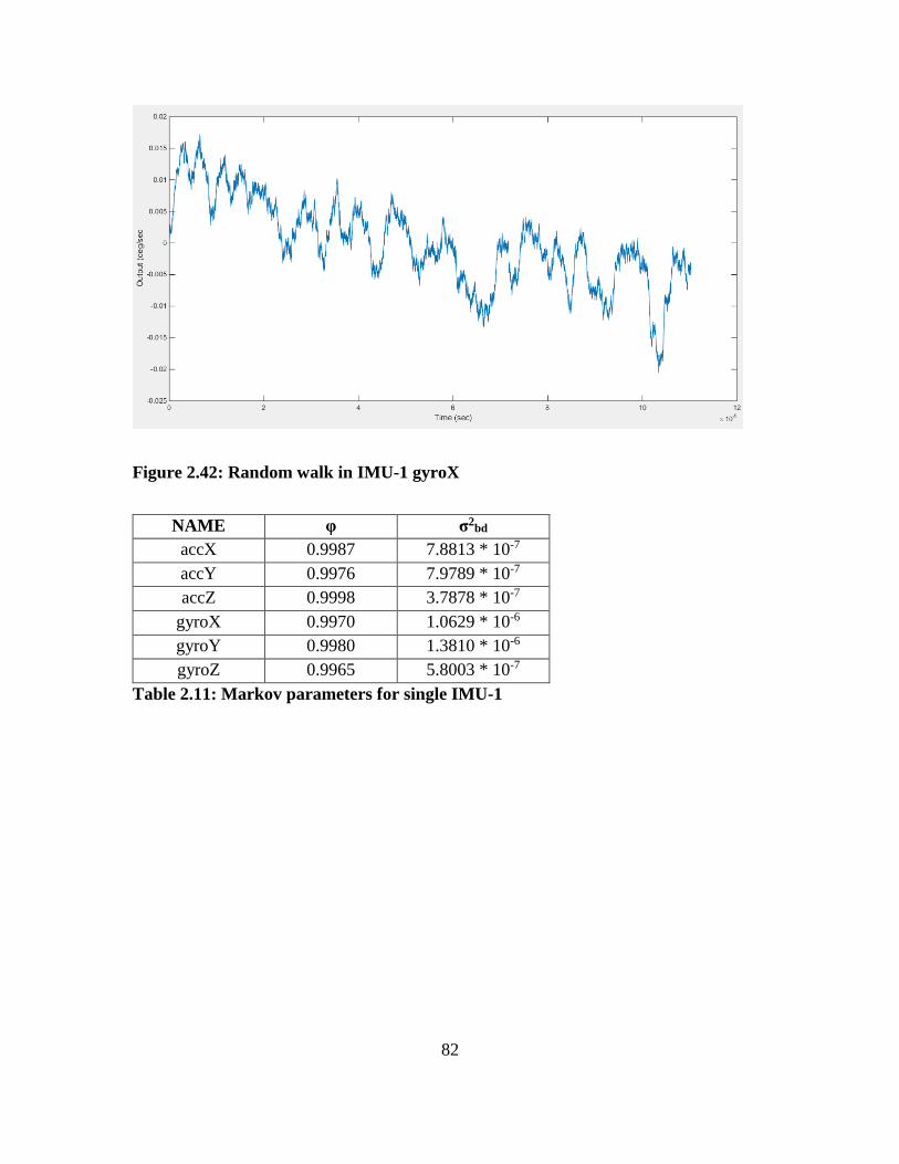
82
Figure 2.42: Random walk in IMU-1 gyroX
NAME φ σ2bd
accX 0.9987 7.8813 * 10-7
accY 0.9976 7.9789 * 10-7
accZ 0.9998 3.7878 * 10-7
gyroX 0.9970 1.0629 * 10-6
gyroY 0.9980 1.3810 * 10-6
gyroZ 0.9965 5.8003 * 10-7
Table 2.11: Markov parameters for single IMU-1

83
Figure 2.43: Random walk in yIMU gyroX
NAME φ σ2bd
accX 0.9997 2.0470 * 10-7
accY 0.9980 4.6136 * 10-7
accZ 0.9997 1.6711 * 10-7
gyroX 0.9969 1.1195 * 10-6
gyroY 0.9965 1.0286 * 10-6
gyroZ 0.9967 3.9966 * 10-7
Table 2.12: Markov parameters for yIMU and comparison to yIMU
From table 2.11 we notice that the effect of drifting bias on gyroscopes is more pronounced
than in accelerometers. In table 2.12 we notice the significant reduction drifting bias in
yIMU due to coupling opposing sense axes. But we note that the effect of drifting bias in
itself is very small in static state (φ is around 1 and σ2bd is very small), but the effect is
definitely more in dynamic state, which needs to be evaluated using techniques outside the
scope of this thesis.

84
From figures 2.42 and 2.43, we notice the reduction in the random walk due to yIMU by
magnitude. To see the remainder of the plots, see appendix B.
2.5.6 Orientation Tracking Performance
Procedure: A manual rotating protractor was used for test 1 to check for pose accuracy. For
tests 2 and 3 a single axis rate table was used.
Figure 2.44: Tracking testing apparatus: (left) manual protractor; (right) single axis rate
table
Test1: Rotate yIMU about z axis: 450 clockwise 600 anticlockwise 600 anticlockwise
Test 2: Around z axis: 300 clockwise, stop for 5 s 300 anticlockwise, stop for 5 s 900
anticlockwise, stop for 5 s 900 clockwise; bringing yIMU to initial position. All rotation
at constant 15 deg/sec.
Test 3: Around z axis: rotate clockwise 1800 at 25 deg/sec rotate anticlockwise 2250 at
30 deg/sec rotate clockwise 250 at 20 deg/sec; bringing yIMU to initial position. Here
the rotation rates are varying to show dynamic performance.

85
Results:
As can be seen in figures 2.44 there is excellent yaw performance of yIMU without any
external aiding. The algorithm is perfect for normal movements to be tracked on human
body. In order to extend the performance of yIMU for higher dynamics more research
needs to be done (see section 4.2). More rigorous testing could be done on a multi-axis
gimbal which requires higher quality instrumentation currently unavailable in the lab.
NOTE: As the protractor is rotated by hand in figure 2.45 we see uneven movement of
yIMU. For figure 2.46 at each change of speed vibration in the motor is picked up by
accelerometer.
Figure 2.45: yaw vs time

86
Figure 2.46: Rate table experiment about yaw axis- constant speed
Figure 2.47: Rate table experiment about yaw axis- varying speed
UNAIDED YAW STABILITY
Stability of yaw in unaided inertial sensors is of concern. yIMU was tested against DMP
algorithm. DMP is a proprietary algorithm from Invensense (InvenSense_Inc. 2013) that
is inbuilt into MPU6050. As can be seen static stability of yIMU-gyroscopes is much

87
superior to DMP with only 0.50 yaw drift in more than an hour compared to around -8.120
drift for DMP in just 20 mins. It should be noted though the roll and pitch of DMP is quite
stable due to aiding by accelerometer. As a comparison we have the drifts for MPU6050
gyroscope raw readings for 20 minutes. This clearly needs a lot of processing. As a
comparison Navigation grade IMUs have a static bias stability of 0.350 /hr.
Figure 2.48: Static stability of yIMU- gyroscopes tested for 1 hour
Figure 2.49: Static stability of MPU6050 with DMP algorithm tested for 20 mins

88
Figure 2.50: Raw gyro output from MPU6050 for 20 minutes: The bias offset has been
compensated.

89
CHAPTER 3
JOINT ANGLE TRACKING USING INERTIAL SENSORS
In this chapter we discuss the development of a motion tracking system. In order to
accurately track human motion precise tracking of joint angles is important. We use the
custom built yIMU as the sensor nodes to track joint segment orientation. Human limb
segment is then modelled as a kinematic chain and joint angle calculations are made.
Though this implementation is for human upper body, it can be further extended to involve
full body motion tracking in future. An experiment to conduct the viability of human
motion tracking was done using MATLAB animation.
3.1 Joint Angle Tracking
This is a simple algorithm to track human body joint angles. Here we had applied to track
motion of human limb. Section 3.1.1 describes the theoretical foundations of the procedure
of kinematical modelling. In section 3.1.2 deals with sensor-segment calibration, which
highly important to align the sensors to body frame and convert sensor orientation readings
from body frame to global frame.
3.1.1 Kinematic Model of Human Limbs
DESCRIBING JOINT MOVEMENT
Human body is a complex system of joints and muscles. In order to study the movement
certain terminologies have been developed with respect to a joint:

90
Figure 3.1: Movements in human joints (Luitz 2013)
1. Flexion and extension- These movements occur in many joints in the body,
including head, trunk, shoulder, elbow, hip and knee. Flexion is a bending
movement that decreases the joint relative angle between two adjacent segments.
Lifting the forearm up at the elbow is an example of elbow flexion. Extension is a
straightening movement that increases the joint relative angle between two adjacent
segments.
2. Abduction and adduction- These movements are not as common as flexion and
extension. They occur in the scapula, shoulder, wrist, and hip joints. Abduction is
a movement away from the midline of the body. Raising an arm out to the side of
the body is an example of abduction. Adduction, on the other hand, is the return
movement of the segment back toward the midline of the body.

91
3. Segment internal and external rotation- They occur in the head, trunk, shoulder, hip
and knee joints. Internal rotation occurs when the segment rotates about the vertical
axis toward the midline of the body. External rotation is the opposite movement
away from the body midline.
4. Pronation and supination- They occur as the distal end of the radius rotates over
and back at the radioulnar joint. While the elbow is flexed, supination occurs in the
forearm when the palm rotates to face upward. Pronation is the opposite movement
to bring the palm back to face downward
Figure 3.2: Categories of joint movements (Pau)
THE CONCEPT OF KINEMATIC CHAIN
Kinematic chain refers to an assembly of rigid bodies connected by joints that is the
mathematical model for a mechanical system (Wikipedia). The degrees of freedom, or
mobility, of a kinematic chain is the number of parameters that define the configuration of
the chain. The DOF for a rigid body free to move in space is 6, hence for n distinct segments
the DOF is 6n. It can be shown that DOF for a kinematic chain formed from n moving
links and j joints each with freedom fi, i=1, ..., j and N fixed links, is given by:

92
𝑴 = 𝟔𝒏 − ∑ (𝟔 − 𝒇𝒊) = 𝟔(𝑵 − 𝟏 − 𝒋) + ∑ 𝒇𝒊𝒋𝒊=𝟏
𝒋𝒊=𝟏
(3.1)
Two or more rigid bodies in space are collectively called a rigid body system. We can
hinder the motion of these independent rigid bodies with kinematic constraints. Kinematic
constraints are constraints between rigid bodies that result in the decrease of the degrees of
freedom of rigid body system. In order to describe the individual motion in series we use
transformation matrices. This procedure is known as forward kinematics formulation. The
transformation matrix T for an n segment kinematic chain with individual matrices
described by Xi, where i=1, ….., n-1 and Zi , where i= 1,…,n is the link transformation
matrix is given by the serial kinematic chain:
[𝑻] = [𝒁𝟏][𝑿𝟏][𝒁𝟐][𝑿𝟐] … … [𝑿𝒏−𝟏][𝒁𝒏] (3.2)
Figure 3.3: Visualizing human body as series of kinematic segments (Wikipedia)
Robotic arms have been developed to mimic human arm dexterity. Hence the system used
in kinematic modelling of robotic arms can in turn be used to mathematically describe

93
human limb. The complex human body can be modeled as a multi-link system comprised
of several body segments. Body segments are thereby treated as rigid bodies and are
mutually connected by joints to form a tree-like structure. The specification of pose of the
body requires that orientations and positions of every individual segment are determined.
Type of formalism chosen to describe relationships between body segments in a model,
determines whether the positions and orientations of the segments are described
individually or are specified relative to one another.
DENAVIT HARTENBERG CONVENTION
In a kinematic model that represents articulated structures as a series of inter-connected
links, the geometrical relationship between links may generally be described using either
homogenous transformation matrices or quaternion/vector pairs. A homogenous
transformation matrix is a 4x4 matrix which expresses both the rotation and translation of
a joint's individual reference frame related to the reference frames of adjacent link.
In DH notation, four parameters are used to describe the relationship between adjacent
frames: link length, link twist, link offset and the joint angle. Every joint with multiple
degrees of freedom can be modeled as an assembly of multiple one-degree-of-freedom
joints and for those joints only changes in joint angle occur. All other parameters are fixed:
d: offset along previous axis of rotation, z to the normal
Ө: angle about the previous z, from old x (part of right handed coordinate system)
to new x
a: length of the common normal
α: angle about the common normal, from old z axis to new z axis
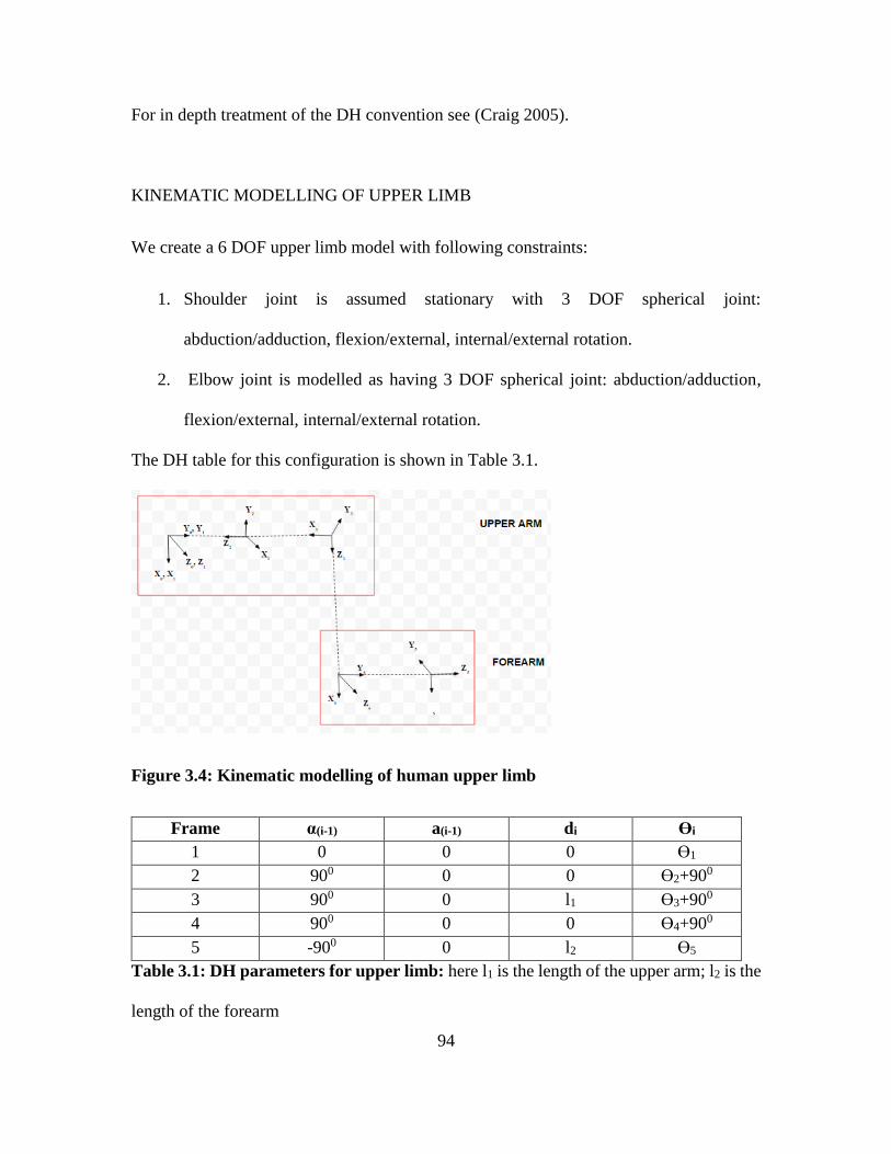
94
For in depth treatment of the DH convention see (Craig 2005).
KINEMATIC MODELLING OF UPPER LIMB
We create a 6 DOF upper limb model with following constraints:
1. Shoulder joint is assumed stationary with 3 DOF spherical joint:
abduction/adduction, flexion/external, internal/external rotation.
2. Elbow joint is modelled as having 3 DOF spherical joint: abduction/adduction,
flexion/external, internal/external rotation.
The DH table for this configuration is shown in Table 3.1.
Figure 3.4: Kinematic modelling of human upper limb
Frame α(i-1) a(i-1) di Өi
1 0 0 0 Ө1
2 900 0 0 Ө2+900
3 900 0 l1 Ө3+900
4 900 0 0 Ө4+900
5 -900 0 l2 Ө5
Table 3.1: DH parameters for upper limb: here l1 is the length of the upper arm; l2 is the
length of the forearm

95
FORWARD KINEMATICS
Once the sensor-segment calibration is done as discussed in section 3.1.2, we have to
implement forward kinematic formulation to calculate the pose of the joints in 3D space.
Now we have to deal with two frames of reference: global frame of reference and body
frame of reference attach at each of the joint as shown in the figure 3.6.
Figure 3.5: Forward kinematics- frames of reference
First we define the orientation calculated at each of the joint: φ1 is the roll calculated at
shoulder (abduction/adduction), Ө1 is the pitch calculated at the shoulder (rotation) and Ѱ1
is the yaw calculated at the shoulder (flexion/extension). We have the similar nomenclature
for elbow orientation: φ1, Ө1 and Ѱ1.
Now we calculate the pose of the point fixed at elbow with respect to global frame 𝒓𝒆𝑮
using the following equation:

96
𝒓𝒆𝑮 = 𝑹𝑩𝟏
𝑮 ∗ 𝒓𝒆𝑩𝟏 (3.3)
where 𝑹𝑩𝟏𝑮 is the rotation matrix for shoulder frame, B1 with respect to global frame, G;
and 𝒓𝒆𝑩𝟏 is the position of elbow with respect to shoulder frame of reference. The rotation
matrix 𝑹𝑩𝟏𝑮 is calculated by using Euler rotation transformation matrix following Z-Y-X
convention.
𝑹𝑩𝟏𝑮 = [
𝒄𝒐𝒔Ѱ𝟏 −𝒔𝒊𝒏Ѱ𝟏 𝟎𝒔𝒊𝒏Ѱ𝟏 𝒄𝒐𝒔Ѱ𝟏 𝟎
𝟎 𝟎 𝟏] ∗ [
𝒄𝒐𝒔Ө𝟏 𝟎 𝒔𝒊𝒏Ө𝟏
𝟎 𝟏 𝟎−𝒔𝒊𝒏Ө𝟏 𝟎 𝒄𝒐𝒔Ө𝟏
] ∗ [
𝟏 𝟎 𝟎𝟎 𝒄𝒐𝒔𝛗
𝟏−𝒔𝒊𝒏𝛗
𝟏
𝟎 𝒔𝒊𝒏𝛗𝟏
𝒄𝒐𝒔𝛗𝟏
]
=[
𝒄𝒐𝒔Ө𝟏 ∗ 𝒄𝒐𝒔Ѱ𝟏 𝒄𝒐𝒔Ѱ𝟏 ∗ 𝒔𝒊𝒏Ө𝟏 ∗ 𝒔𝒊𝒏𝛗𝟏
− 𝒄𝒐𝒔Ө𝟏 ∗ 𝒔𝒊𝒏Ѱ𝟏 𝒔𝒊𝒏𝛗𝟏
∗ 𝒔𝒊𝒏Ѱ𝟏 + 𝒄𝒐𝒔𝛗𝟏
∗ 𝒄𝒐𝒔Ѱ𝟏𝒔𝒊𝒏Ө𝟏
𝒄𝒐𝒔Ө𝟏 ∗ 𝒔𝒊𝒏Ѱ𝟏 𝒄𝒐𝒔𝛗𝟏
∗ 𝒔𝒊𝒏Ѱ𝟏 + 𝒔𝒊𝒏Ө𝟏 ∗ 𝒔𝒊𝒏𝛗𝟏
∗ 𝒔𝒊𝒏Ѱ𝟏 𝒄𝒐𝒔𝛗𝟏
∗ 𝒔𝒊𝒏Ө𝟏 ∗ 𝒔𝒊𝒏Ѱ𝟏 − 𝒄𝒐𝒔Ѱ𝟏 ∗ 𝒔𝒊𝒏𝛗𝟏
−𝒔𝒊𝒏Ө𝟏 𝒄𝒐𝒔Ө𝟏 ∗ 𝒔𝒊𝒏Ѱ𝟏 𝒄𝒐𝒔𝛗𝟏
∗ 𝒄𝒐𝒔Ө𝟏
]
(3.4)
Next we calculate the pose of the point fixed at the end of forearm (at the wrist) as follows:
𝒓𝑾𝑮 = 𝒓𝑬
𝑮 + 𝒓′𝑾𝑮 (3.5)
where 𝒓𝑾𝑮 is the pose of the wrist with respect to global frame; 𝒓𝑬
𝑮 is the pose of the elbow
joint as calculated previously and 𝒓′𝑾𝑮 is the pose of the wrist with respect to global frame
without taking into account that it is attached to elbow.

97
𝒓′𝑾𝑮 is calculated based on the following equation:
𝒓𝒆𝑮 = 𝑹𝑩𝟏
𝑮 ∗ 𝑹𝑩𝟐𝑩𝟏 ∗ 𝒓𝒘
𝑩𝟐 (3.6)
where 𝑹𝑩𝟏𝑮 is the rotation matrix for B1 with respect to G (as calculated before); 𝑹𝑩𝟐
𝑩𝟏 is the
rotation matrix for B2 with respect to B1; and 𝒓𝒘𝑩𝟐 is the position of wrist with respect to
frame B2.
3999
JOINT ANGLE CALCULATIONS
The shoulder joint angles can be readily calculated by the matrix 𝑹𝑩𝟏𝑮 as the shoulder joint
is assumed fixed. The calculation of elbow joint angle in 3D reduces to finding the angle
between vectors in 3D space. We use the cosine rule:
�̅�. �̅� = 𝒂𝒃 𝐜𝐨𝐬 (Ө) (3.7)
The pose of the upper arm is given by 𝒓𝒆𝑮 and the pose of the forearm is given by 𝒓𝑾
𝑮 . Hence
first we normalize the vectors 𝒓𝒆𝑮 and 𝒓𝑾
𝑮 and then use the equation:
Ө = 𝐚𝐜𝐨𝐬(𝒓𝟏. 𝒓𝟐) (3.8)
where 𝒓𝟏 =𝒓𝒆
𝑮
|𝒓𝒆𝑮|
and 𝒓𝟐 = 𝒓𝑾
𝑮
| 𝒓𝑾𝑮 |
and Ө is the elbow joint angle.

98
3.1.2 Sensor-Segment Calibration
The attachment of sensor to segment may not be perfect. It is important to have them
aligned if the system has to work. A simple way is to use a pre-determined pose to initialize
the adjustment along with the fact that gravity always points down in the global frame.
We make the subject stand straight for a period of 30 s at the beginning of the experiment
to do his alignment. In order to have better accuracy, the subject is instructed to be as still
as possible. This is used to determine the rotation matrix R which is the rotation matrix of
sensor to segment frame. The known gravity component G is aligned with the segment
frame by making the subject stand hands down and straight. If B is the body frame in a
particular pose, we then have:
G= R x B (3.9)
This matching of sensor frame to global frame is done using least square iteration (Hamdi,
Mohammed I. Awad et al. 2014). Once we have determined R from the above equation we
use it for transforming orientation measurements in sensor frame to segment frame as
follows:
[𝒂𝒔𝒙 𝒂𝒔𝒚 𝒂𝒔𝒛]′ = 𝑹 𝒙 [𝒂𝒃𝒙 𝒂𝒃𝒚 𝒂𝒃𝒛]′ for accelerometers ( 3.10)
[𝒈𝒔𝒙 𝒈𝒔𝒚 𝒈𝒔𝒛]′ = 𝑹 𝒙 [𝒈𝒃𝒙 𝒈𝒃𝒚 𝒈𝒃𝒛]′ for gyroscopes (3.11)
Where [𝒂𝒔𝒙 𝒂𝒔𝒚 𝒂𝒔𝒛 𝒈𝒔𝒙 𝒈𝒔𝒚 𝒈𝒔𝒛 ] are sensor outputs in the segment frame;
[𝒂𝒃𝒙 𝒂𝒃𝒚 𝒂𝒃𝒛 𝒈𝒃𝒙 𝒈𝒃𝒚 𝒈𝒃𝒛 ]are the sensor outputs in the sensor frame of reference; and
R is the rotation matrix.

99
Figure 3.6: Sensor-segment calibration
3.1.3 System Design
The system consists of yIMU as sensor nodes that are firmly attached to human limb
segments. The orientation data is sent to the main hub (computer) via Bluetooth. The range
of Bluetooth is 10 m. The logged data is processed off line to calculate joint angles by
applying the kinematic concepts developed earlier. This processing is done on MATLAB.
Figure 3.7: Tracking system design

100
3.2 Performance Evaluation
In this section we evaluate the performance of the inertial tracking algorithm as applied to
yIMU. In 3.2.1 the experimental procedure to validate the system has been documented. In
section 3.2.2 we discuss the conclusions drawn from the results and some improvements
for further development of the joint angle tracking system.
3.2.1 Experiment
The system was setup with IMUs mounted on upper arm and lower arm as shown in figure
3.8. The initial few seconds the subject was asked to remain still for sensor-segment
calibration, then the subject was directed to move arms in any pattern. While the data was
being wirelessly logged via Bluetooth on computer, a camera simultaneously recorded the
movements.
The forward kinematic technique previously discussed was implemented in MATLAB and
used to calculate joint angles. The accuracy was tested using Noraxon IMUs. The best
RMSE was found to be 2.7308 for shoulder adduction/abduction calculations, it varied to
as high as 18.230 (for fast movements) for elbow flexion. The table 3.2 shows the result of
these tests for each of the angles.
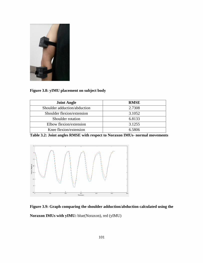
101
Figure 3.8: yIMU placement on subject body
Joint Angle RMSE
Shoulder adduction/abduction 2.7308
Shoulder flexion/extension 3.1052
Shoulder rotation 6.8133
Elbow flexion/extension 3.1255
Knee flexion/extension 6.5806
Table 3.2: Joint angles RMSE with respect to Noraxon IMUs- normal movements
Figure 3.9: Graph comparing the shoulder adduction/abduction calculated using the
Noraxon IMUs with yIMU: blue(Noraxon), red (yIMU)

102
Figure 3.10: Graph comparing the shoulder rotation calculated using the Noraxon
IMUs with yIMU
Figure 3.11: Graph comparing the elbow flexion angle calculated using the Noraxon
IMUs with yIMU
Figure 3.12: Graph comparing the knee flexion angle calculated using the Noraxon
IMUs with yIMU

103
3.2.2 Results and Discussion
As a result of the above experiments we can conclude that yIMU can be adequately used
for human motion tracking. It is to be noted that no external aiding sensors were used. The
tracking was processed off-line. The tracking algorithm is stable over a long period of time
and accurate for a wide range of motions even without magnetometer aiding typically used
for yaw angle calculations. The orientation tracking performance evaluated in section 2.5.6
points to promising results from such an experiment. In addition, for better motion tracking
performance it would be priority to reduce the form-factor of the IMU for easy and firm
mounting on the body segments. This would definitely be implemented in future work. If
allowances for misalignment errors due to the bulky nature of the prototype were to be
made, it is highly possible to have average RMSE below 3 deg.
The commerciality of the device has hence been thoroughly established for human motion
tracking application. This low-cost system costs less than $15 and has great potential for a
wide range of applications.

104
Chapter 4
CONCLUSION
The initial motivation of the thesis was to develop an efficient joint angle tracking
algorithm using rigid kinematic constraints. But while working on this, a sore need for
increasing the raw performance of inertial sensors were noted. Hence the bulk of the work
focusses of development of a new attitude reference system using inertial sensors.
Experiments were carried out to prove the applicability of a dual IMU system to improve
noise performance. Adequate processing of the raw inertial data was done to arrive at
unprecedented stability in inertial sensor readings unaided by any external sensors. An
efficient joint angle tracking algorithm was implemented to track human motion which can
be further extended to development of a motion capture system.
Key areas of further improvements were identified and the work to take yIMU to the next
level is already under process.
4.1 Contributions
The most important contribution of this research is to prove the applicability of low-cost
inertial measurement unit to tracking human motion with precision. To the best of author’s
knowledge, no other custom built low-cost IMU unaided by magnetometer has been
demonstrated to show such accuracy. This quest to not use magnetometer was inspired by
the important problem of magnetic interference in indoor environments. In addition, yIMU
outputs accurate quaternions/ Euler angles as against raw data which is done my most of
the low cost systems in market. This simplifies the post-processing scheme.

105
The following is the summary of the results that form the core of the thesis:
1. Common Mode Effect is highly dependent on the type on sensor used. MPU6050
is a low-cost sensor with repeatable characteristics that can take advantage of this
effect in a particular configuration.
2. Testing for viability of improvements in measurements just by using this
configuration has been proven to be true. Tests were done to see improvements in
noise performance and effect of environmental factors.
3. Exceptionally good unaided yaw performance was tested by virtue of significant
improvements in gyro performance of yIMU.
4. The system was built on an open source platform with very low processing power
pointing to the fact that much better units could be built with good commercial
scalability.
5. Used for joint angle tracking with much better results than similar systems, hence
the use of yIMU in motion capture systems is validated.
On the basis of yIMU, a human motion tracking system was built from scratch. A very
streamlined algorithm was developed which underscores the possibility of smartly
implementing simple techniques for much greater improvements in accuracy instead of
relying on standard Kalman filtering techniques. This shows that sensor fusion only works
best if the theory behind the processes is thoroughly understood and implemented instead
of using a standard algorithm blindly. This understanding enabled the development of a
computationally efficient system with great potential.

106
4.2 Future Work
This thesis presents an effective device to bring down the cost of inertial human motion
tracking systems that are currently in market. Applications to joint angle tracking and
pedestrian navigation was explored here but the scope of application is much huge,
especially in the wearable medical devices market.
With enough funding and dedicated team of developers this system could be hugely
improved:
1. Exhaustive characterization of low-cost IMUs need to be done to take into all the
errors. This is very time-consuming.
2. Further development of dynamic stability of yIMU is needed. This would increase
the scope of application to tracking highly dynamic sports like baseball and
running. One idea would be to include addition sensors to create a larger sensor
array. This would require sophisticated research into efficient geometric
configurations to implement a skew-redundant system.
3. A more elaborate calibration routine would enable yIMU to come closer to the
performance of tactical grade inertial sensors. This would require accurate
compensation for scale factor error, misalignment error and development of an on-
line bias estimation routine.
4. Hardware development of the IMU. Funding and adequate expertise in embedded
systems has been a huge impediment in development of the device. Implementation
of any stochastic algorithm or sophisticated bias estimation would require more

107
powerful hardware options. The commerciality of the concept though has been
thoroughly established.
5. As far as the joint angle tacking algorithm is concerned, no velocity constraints
were applied and the implementation was not done in state-space form. On testing,
it was concluded that such implementations work best only by using Kalman filter.
A preliminary EKF filter using velocity constraints was built (not included in the
thesis), but the results were not encouraging. This implied the design needs more
elaborate error modelling scheme than what was used in this thesis in addition to
better processor speeds on the hardware side. The concept though is very useful
and will be fruitfully pursued for future improvements.
6. Exhaustive testing for medical applications has not been done. Human
rehabilitation studies needed to implement a more robust sensor to segment
calibration routine. Using UKF for joint angle tracking could be a more lucrative
choice. More research needs to be done in this area.
7. Building a real-time system heavily depends on the usage of better hardware and
friendly UI development.
8. Building a new IMU with magnetometer and appropriate distortion correction
algorithms would be very handy for many applications. yIMU can be integrated
into any system that requires inertial tracking. This is a 6DOF system on chip with
inbuilt smart sensor fusion that can give accurate orientation without magnetometer
aiding for longer durations of time than any current low-cost sensor. This could
prove to be useful when external aiding sensors cannot be trusted due to various
factors that can be accordingly modelled into a robust fault detection scheme.

108
9. yIMU has wide ranging applications and can be easily integrated for DIY projects,
the following list is of some major applications:
a. Motion capture, activity and other human tracking applications.
b. Gesture control, head tracking and other gaming applications.
c. Pedestrian navigation.
d. Orientation control in drones
All these applications would require more complex algorithm with domain specific
constraints which require extensive research.

109
REFERENCES
Aggarwal, P., et al. (2006). Cost-effective Testing and Calibration of Low Cost MEMS
Sensors for Integrated Positioning, Navigation and Mapping Systems Shaping the
Change XXIII FIG Congress. Munich, Germany.
Allan, D. W. (1966). Statistics of atomic frequency standards. Proceedings of the IEEE.
Alvarez, H. D. E. (2010). Geometrical Configuration of Redundant Inertial Measurement
Unit. Department of Mechanical Engineering, University of Texas at Austin. Master of
Science.
Analog_Devices. "ADIS16365 product overview ". from
http://www.analog.com/en/products/sensors/inertial-measurement-
units/adis16365.html#product-overview.
Bancroft, J. B. and G. Lachapelle (2011). "Data Fusion Algorithms for Multiple Inertial
Measurement Units " Sensors.
Barrett, J., et al. (2012). "Analyzing and Modelling an IMU for Use in a Low-Cost
Combined Vision and Inertial Navigation System." IEEE: 21-22.
Benoussaad, M., et al. (2016). "Robust Foot Clearance Estimation Based on the
Integration of Foot-Mounted IMU Acceleration Dat." Sensors: 3-6.
CH_Robotics. "Understanding Euler Angles."
Craig, J. J. (2005). Introduction to robotics, Pearson Prentics Hall.
eLegs (2010). from
http://bleex.me.berkeley.edu/research/exoskeleton/elegs%E2%84%A2/.
El-Gohary, M. and J. McNames (2015). "Human Joint Angle Estimation with Inertial
Sensors and Validation with a Robot Arm." IEEE Transactions on Biomedical
Engineering 62(7): 1759-1766.
Fourati, H., et al. (2013). "A Complementary Sliding Mode Observer Approach for
Motions Human Body Segments Capturing by Means of Wearable Inertial and Magnetic
MEMS Sensors Assembly." IEEE/ASME Transactions on Mechatronics.
110
Greenheck, D. R., et al. (2014). Design and Testing of a Low-Cost MEMS IMU Cluster
for SmallSat Applications. 28th Annual AIAA/USU Conference on Small Satellites.
Logan, Utah: 6-8.
Grewal, M. S., et al. (2001). global positioning systems inertial navigation and
integration, Wiley-Ineterscience.
Groves, P. D. (2013). Principles of GNSS, Inertial, and Multisensor Integrated
Navigation Systems, Arctech House.
Hamdi, M. M., et al. (2014). Lower Limb Motion Tracking Using IMU Sensor Network.
Cairo International Biomedical Engineering Conference Cairo, Egypt.
Hol, J. (2011). Sensor Fusion and Calibration of Inertial Sensors, Vision, Ultra-Wideband
and GPS. Department of Electrical Engineering, Linkoping University Doctor of
Philosophy.
Hong, S. K. and S. Park (2008). "Minimal-Drift Heading Measurement using a MEMS
Gyro for Indoor Mobile Robots." Sensors: 7295-7296.
Innoventions. "Accelerometers." from http://www.rotoview.com/accelerometer.htm.
InvenSense_Inc. (2013). MPU-6000 and MPU-6050 Product Specification Revision 3.4.
Kanjanapas, K., et al. (2013). "A Human Motion Capture System based on Inertial
Sensing and a Complementary Filter." ASME: 3-6.
Kavanagh, J. J., et al. (2006). "Reliability of segmental accelerations measured using a
new wireless gait analysis system." Journal of Biomechanics.
Kerestes, J. (2014). Robotic Augmentation Of Human Locomotion For High Speed
Running. Department of Mechanical Engineering, Arizona State University. Master of
Science.
Koldbæk, S. K. and L.-C. Totu (2011). Improving MEMS Gyroscope Performance using
Homogeneous Sensor Fusion. Department of Electronic Systems, Aalborg University.
Master of Science: 61-64.

111
Kong, K. and M. Tomizuk (2009). "A Gait Monitoring System Based on Air Pressure
Sensors Embedded in a Shoe." IEEE/ASME Transactions on Mechatronics 4(3).
KVH_Industries (2014). Guide to Comparing Gyro and IMU Technologies- MEMS and
FOGs, .
Kwakkel, S. P. (2008). Human Lower Limb Kinematics Using GPS/INS. Department of
Geomatics Engineering, Schulich School of Engineering. Master of Science.
Looney, M. "The Basics of MEMS IMU/Gyroscope Alignment." from
http://www.analog.com/library/analogdialogue/archives/49-06/IMU_Gyroscope.html.
lubopitko-bg. "Joint Articulations." from http://encyclopedia.lubopitko-
bg.com/Joints_Articulations.html.
Luitz, E. G. (2013). "Practical Anatomy." from
http://www.drawingbooks.org/lutz1/source/index.html.
Martin, H. and P. Groves (2016). "The Limits of In-Run Calibration of MEMS Inertial
Sensors and Sensor Array." Journal of The Institute of Navigation.
Martin, H., et al. (2013). A new approach to better low-cost MEMS IMU performance
using sensor arrays. I. o. N. GNSS. Nashville,TN,USA: 3-7.
Masters, M., et al. (2015). "Real-Time Arm Tracking for HMI Applications." IEEE.
Nilsson, J. O. and I. Skog (2016). Inertial sensor arrays – A literature reviewin
Proceedings of European Navigation Conference. Helsinki, Finland.
NXP. "NXP Sensor Fusion." from http://www.nxp.com/products/sensors/nxp-sensor-
fusion:XTRSICSNSTLBOX.
Paina, G. P., et al. (2011). Experimental comparison of Kalman and complementary filter
for attitude estimation. Argentine Symposium on Technology. Cordoba, Argentina.
Pau. "Pau's Medical Biology Notes." from
https://pausmedicalbiologynotes.wordpress.com/tag/anatomy/.
Pedley, M. (2013). Tilt Sensing Using a Three-Axis Accelerometer, Freescale
Semiconductors.

112
PerceptionNeuron. "What is Motion Capture." from
https://neuronmocap.com/content/mocap-101.
Quoc, D. D., et al. (2015). "Attitude Estimation Algorithms Using Low-Cost IMU."
International Journal of Control and Automation: 117-119.
Roetenberg, D., et al. (2013). Xsens MVN: Full 6DOF Human Motion Tracking Using
Miniature Inertial Sensors, Xsens Technologies.
Roetenberg, D., et al. (2005). "Compensation of Magnetic Disturbances Improves Inertial
and Magnetic Sensing of Human Body Segment Orientation." IEEE Transactions on
Neural Systems and Rehabilitation Engineering.
Scapello, S., et al. (2005). "In-use calibration of body-mounted gyroscopes for
applications in gait analysis." Sensors and Actuators.
Shiau, J.-K., et al. (2012). "Noise Characteristics of MEMS Gyro’s Null Drift and
Temperature Compensation." Journal of Applied Science and Engineering.
Skog, I., et al. (2016). "Inertial Sensor Arrays, Maximum Likelihood, and Cram´er-Rao
Bound." IEEE.
Slifka, L. D. (2004). An Accelerometer Based Approach to Measuring Displacement of a
Vehicle Body. Department of Electrical and Computer Engineering, University of
Michigan: 19-23.
Taunyazov, T., et al. (2016). A Novel Low-Cost 4-DOF Wireless Human Arm Motion
Tracker. 6th IEEE RAS/EMBS International Conference on Biomedical Robotics and
Biomechatronics (BioRob). UTown, Singapore.
Tedaldi, D., et al. (2013). "A Robust and Easy to Implement Method for IMU Calibration
without External Equipments."
Titterton, D. and J. Weston (2004). Strapdown Inertial Technology. The Institution of
Engineering and Technology.
Unsal, D. and K. Demirbas (2012). "Estimation of Deterministic ans Stochastic IMU
Error Parameters." IEEE.

113
VectorNav. "Inertial Measurement Units." from
http://www.vectornav.com/support/library/imu-and-ins.
Wikipedia. "Kinematic Chain." from https://en.wikipedia.org/wiki/Kinematic_chain.
Woodman, O. J. (2007). An introduction to inertial navigation, University of Cambridge.
Yuksel, Y. (2011). Design and Analysis of Inertial Navigation Systems with Skew
Redundant Inertial Sensors, Schulich School of Engineering. Doctor of Philosophy.
Yuksel, Y., et al. (2010). "Error Modelling and Characterization of Environmental
Effects for Low Cost Inertial MEMS Units
" IEEE: 605-611.
Zhang, W., et al. (2014). A Wireless Human Motio Monitoring System Based on Joint
Angle Sensors and Smart Shoes. ASME Dynamic Systems and Control Conference
Zhao, Y. (2011). GPS/IMU Integrated System for Land Vehicle Navigation based on
MEMS. Division of Geodesy and Geoinformatics, Royal Institute of Technology (KTH).
Master of Science.
Zhi, R. (2016). A Drift Eliminated Attitude and Position Estimation Algorithm in 3D.
Electrical Engineering, University of Vermont. Master of Science: 31-35.

114
APPENDIX A
MATHEMATICAL RESULTS

115
The following are some more discussion of the mathematics relevant to the thesis:
A1. Allan Variance
A2. Markov Process Model
A3. ACF calculation
A4. Normal Distribution
A1. Allan Variance
This method was developed to analyze the signal in time-series to characterize all the errors
in a single graph. The following equation describes the process:
𝜎2(𝑛𝑇) =1
2(𝑁 − 1)∑(𝑦𝑖+1 − 𝑦𝑖)
2
𝑁−1
𝑖=1
where г is the sampling time; xi are the samples collected over a large time span; n is the
size of the bin such that N is the total number of bins and yi is the average of bin i. The
curves are known as Allan deviation curves which is square root of Allan variance.
The idea is to glean sensor performance characteristics from data by averaging over a range
of time spans. This averaging leads to removal of noise systematically from the sample
data revealing effects of different noise sources on the sensor measurements. It gives us an
idea of how well noise correction could be achieved under ideal conditions i.e. when there
is no temperature variations or any external disturbances. In particular, it gives a measure
of frequency stability of how good the noise correction could be. To make the interpretation

116
of the graphs easier, usually the Allan deviation curves are plotted as they are in the same
units as the data collected making it easy for comparison.
A more detailed deconstruction of Allan deviation plot is:
But for our analysis we have used only four points in the graph:
1. Point A: This is the starting point of the graph that represents standard deviation of
noise for any one single measurement point. This gives us an idea of how noisy a
single measurement could be; it is to be noted that this mentions the probability of
noisy measurements not the certainty of it. The value tells you that 68% of the
measurements will have the noise as stated in the y axis and the remainder will have
noise greater than that. This is useful to compare if the noise will be a significant
part of the measurements.
2. Slope A: This is the slope for the first part of the AV graph before the dip. This part
is used to analyze the measurement noise, that depends on the influence of high
frequency errors. This is as the averaging span in this region is still lot smaller,
hence high frequency errors will dominate the calculations. These errors involve
117
quantization error and measurement errors. For the purpose of this thesis we have
focused only on the measurement errors.
3. Point B: Represents the bias stability of the sensor. It gives you the lowest possible
value of bias error generated in a sensor. This minimum point is go when
theoretically the effect of high frequency errors and low frequency errors balance
out to give the best possible value possible by the sensor. The lower the value, the
better sensor it is. This is usually the main performance characteristic of a sensor,
especially the gyroscopes.
4. Slope B: This is the slope for the second part of the AV graph, after the dip. This
part is used to analyze the random walk errors, that depends on the influence of low
frequency errors. This usually consists of the rate random walk and the rate ramp
effect. For this thesis we only confirm the random nature of these noise sources.
In addition, to this these plots can be used to compare the effect of temperature on readings,
which has not been explored here. We used the plot to identify the nature of the noise i.e.
is the measurement noise is white or not. This is important so that the bias term in the error
equation used is modelled as Gaussian White Noise. It has been further confirmed by the
PSD and PDF analysis done further in the thesis.
A2. Markov Process Model
A random process is a time sequence representing the evolution of some system
represented by a variable whose change is subject to a random variation. For discrete time,
a stochastic process is a sequence of random variables, which is usually the case with digital

118
signals; with the only requirement that these random variables be part of the same space.
A way to describe such a process is Markov Model. A stochastic process is called Markov
if for every random variable n in a time series, we have:
𝑃(𝑥(𝑡𝑛) ≤ 𝑥𝑛 = |𝑥(𝑡) 𝑓𝑜𝑟 𝑎𝑙𝑙 𝑡 ≤ 𝑡𝑛 − 1
= 𝑃(𝑥(𝑡𝑛) ≤ 𝑥𝑛|𝑥(𝑡𝑛−1))
This model is widely used for modelling sensor errors, not only because it is able to
represent a large number of physical processes, but also because it has comparatively a
straightforward mathematical equation. The continuous model for this process is depicted
as follows:
�̇� =1
𝑇𝑥 + 𝑤
where x is the random process with zero mean, T and noise w.
From this we can have the discrete form equation:
𝑥𝑖 = (1 − ℰ𝑑𝑡)𝑥𝑖−1 + 𝑤𝑖
where dt is the sampling time and 𝑤𝑖 is the white noise with noise covariance given by:
𝜎𝑤𝑖
2 = 𝜎𝑥𝑖
2 (1 − 𝑒−2𝑑𝑡
𝑇 )
the value for T and 𝜎𝑥𝑖
2 could be found from Allan variance plot. Then the parameters can
be implemented in the Kalman filter.
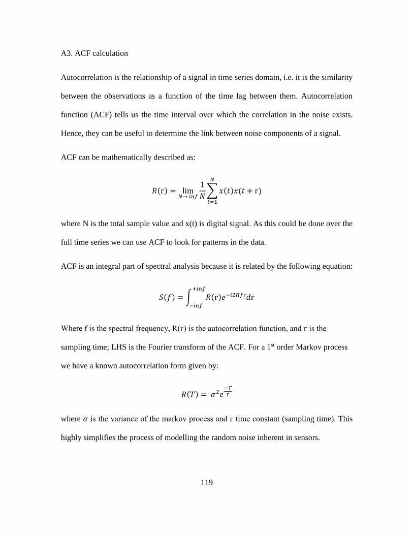
119
A3. ACF calculation
Autocorrelation is the relationship of a signal in time series domain, i.e. it is the similarity
between the observations as a function of the time lag between them. Autocorrelation
function (ACF) tells us the time interval over which the correlation in the noise exists.
Hence, they can be useful to determine the link between noise components of a signal.
ACF can be mathematically described as:
𝑅(г) = lim𝑁→ 𝑖𝑛𝑓
1
𝑁∑ 𝑥(𝑡)𝑥(𝑡 + г)
𝑁
𝑡=1
where N is the total sample value and x(t) is digital signal. As this could be done over the
full time series we can use ACF to look for patterns in the data.
ACF is an integral part of spectral analysis because it is related by the following equation:
𝑆(𝑓) = ∫ 𝑅(г)𝑒−𝑖2𝛱𝑓г𝑑г+𝑖𝑛𝑓
−𝑖𝑛𝑓
Where f is the spectral frequency, R(г) is the autocorrelation function, and г is the
sampling time; LHS is the Fourier transform of the ACF. For a 1st order Markov process
we have a known autocorrelation form given by:
𝑅(𝑇) = 𝜎2𝑒−𝑇
г
where 𝜎 is the variance of the markov process and г time constant (sampling time). This
highly simplifies the process of modelling the random noise inherent in sensors.

120
A4. Normal Distribution
Normal distribution also known as the Gaussian Distribution, is a kind of probability
distribution used to describe a sample of real-valued variables. It is represented by the
following equation:
𝑓(𝑥) =1
√2𝛱𝜎2𝑒
−(𝑥−ϻ)2
2𝜎2
where ϻ is the mean and 𝜎2 is variance of distribution x. The figure below depicts the
graphical form of the distribution which distinctly appears as a ‘bell’.
The distribution is designed such that the bulk of the sample are present in the region
surrounding the mean within 1 standard deviation (68% of the area) and the total area of
the curve is equal to 1. 95% of the area falls into 2 standard deviations and 99.7% fall
within 3 standard deviations. The term standard deviation is a measure that is used to
quantify the amount of variation of sample set.
Standard deviation can be approximately described with the following equation:

121
𝜎 =1
𝑁√∑(𝑥𝑖 − ϻ)2
𝑁
𝑖=1
where 𝜎 is the standard deviation, N is the total number of samples; 𝑥𝑖 is the ith sample
and ϻ is the mean. Another useful term is variance, defined as the square of standard
deviation:
𝑣𝑎𝑟 = 𝜎2
It is especially useful in mathematical manipulations as it is a positive number unlike the
standard deviation (which is a square root). This term is the measure of dispersion of data
with respect to mean of the sample. The unit of variance is square of standard deviation,
hence for comparison purposes usually standard deviation is used.
The usefulness of normal distribution is due to the central limit theorem, which states that
averages of random variables independently drawn from independent distributions
converge in distribution to the normal, that is, become normally distributed when the
number of random variables is sufficiently large. Hence it can easily describe a variety of
physical phenomena accurately.

122
APPENDIX B
STATIC TEST PLOTS

123
The following are the results of the static test data:
B1. Allan Deviation
B2. Power Spectral Density
B3. Probability Density Function
B4. Drifting Bias
Static test was done for a period of 12 hours on yIMU in a thermal chamber. Care was
taken so that the test unit was left untouched and no external impulses were given to it.
B1. Allan Deviation
The following section has the AV plots and the corresponding points of interest in the
tables. The plots were generated in AlaVar 5.2. X axis unit: sec; Y axis unit (deg/sec) for
gyroscopes and m/s2 for accelerometers.
IMU-1 accelerometer X

124
IMU-1 accelerometer Y
IMU-1 accelerometer Z
POINT A
(g)
SLOPE A
POINT B
(g)
SLOPE B
IMU-1 X 0.07 -0.483754 0.0057 0.313607
IMU-1 Y 0.07 -0.519263 0.0035 0.149470
IMU-1 Z 0.07 -0.464424 0.00480 0.280849

125
IMU-1 gyroscope X
IMU-1 gyroscope Y
IMU-1 gyroscope Z

126
POINT A
(deg/s)
SLOPE A
POINT B
(deg/s)
SLOPE B
IMU-1 X 0.07 -0.51176 0.0053 -0.40475
IMU-1 Y 0.07 -0.522333 0.0042 -0.40306
IMU-1 Z 0.07 -0.527713 0.0026 0.28838
yIMU accelerometer X
yIMU accelerometer Y
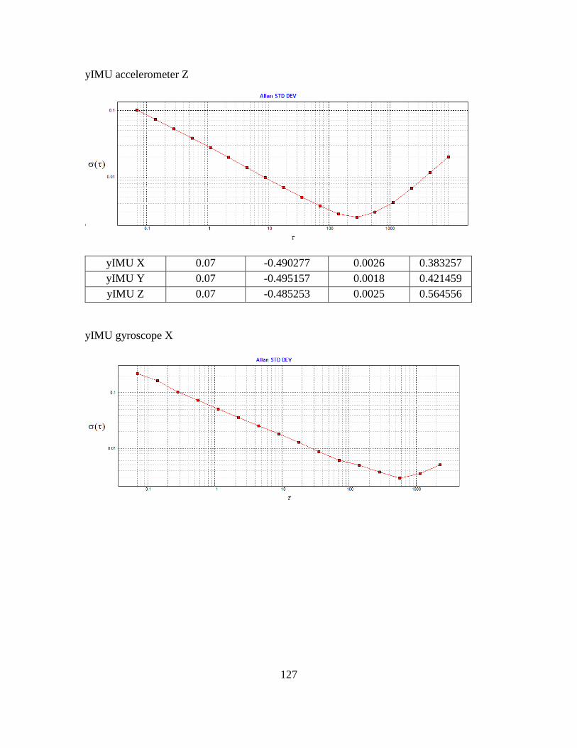
127
yIMU accelerometer Z
yIMU X 0.07 -0.490277 0.0026 0.383257
yIMU Y 0.07 -0.495157 0.0018 0.421459
yIMU Z 0.07 -0.485253 0.0025 0.564556
yIMU gyroscope X

128
yIMU gyroscope Y
yIMU gyroscope Z
yIMU X 0.07 -0.519355 0.0029 0.484973
yIMU Y 0.07 -0.505054 0.0025 -
yIMU Z 0.07 -0.514046 0.0023 0.476239
B2. Power Spectral Density
The following are the PSD graphs generated in AlaVar 5.2. Unit of Y axis: (m/s2)2/Hz2
(accelerometers) and (deg/sec)2/Hz2.

129
IMU-1 accelerometer X
IMU-1 accelerometer Y
IMU-1 accelerometer Z

130
IMU-1 gyroscope X
IMU-1 gyroscope Y
IMU-1 gyroscope Z

131
yIMU accelerometer X
yIMU accelerometer Y
yIMU accelerometer Z

132
yIMU gyroscope X
yIMU gyroscope Y
yIMU gyroscope Z
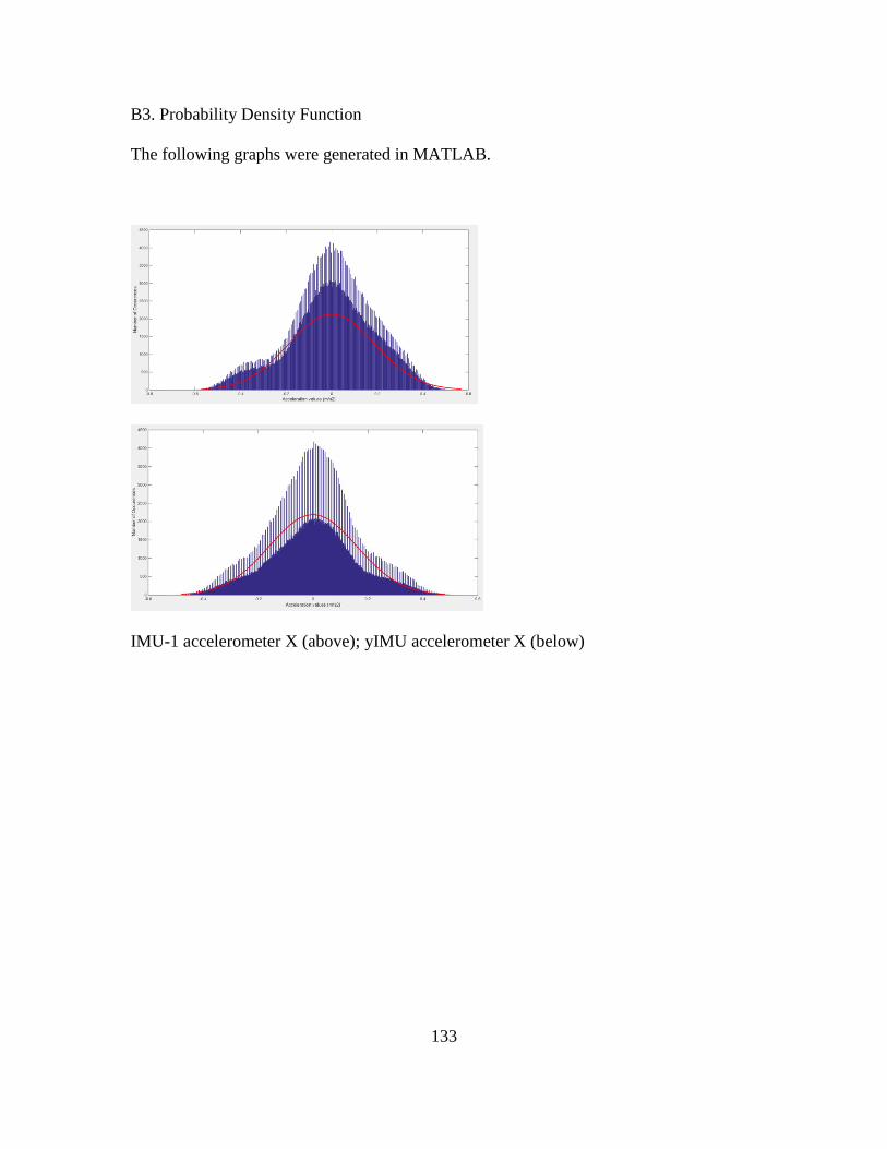
133
B3. Probability Density Function
The following graphs were generated in MATLAB.
IMU-1 accelerometer X (above); yIMU accelerometer X (below)

134
IMU-1 accelerometer Y (above); yIMU accelerometer Y (below)

135
IMU-1 accelerometer Z (above); yIMU accelerometer Z (below)
IMU-1 gyroscope Y yIMU gyroscope Y
IMU-1 gyroscope Z yIMU gyroscope Z
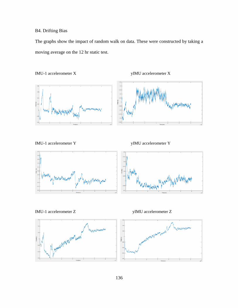
136
B4. Drifting Bias
The graphs show the impact of random walk on data. These were constructed by taking a
moving average on the 12 hr static test.
IMU-1 accelerometer X yIMU accelerometer X
IMU-1 accelerometer Y yIMU accelerometer Y
IMU-1 accelerometer Z yIMU accelerometer Z