1

2

Robust Design for a Long-Range Strategic Missile System

Ryan Ogilvie1, Casey Wilson1, Jeff Pattison1, Rahul Rameshbabu1, Andrew Van Zwieten1, William Craver2

Aerospace Systems Design Laboratory, Georgia Institute of Technology, Atlanta, GA, 30332, USA

This paper outlines the design procedure for a long-range strategic missile system that can meet

all of the required performance parameters specified in the request for proposal from the customer.

By performing a design of experiments and integrating various engineering disciplines, the final

missile designed has the capability to reach targets as far as 10680 nmi. With this design, it is

ensured that the United States retains the status as a nuclear power, guaranteeing mutually assured

destruction.

I. Nomenclature

dt = time step

cg = center of gravity

𝑐𝑐𝑝𝑝𝑚𝑚𝑚𝑚𝑚𝑚 = specific heat of a solid material (Btu/lbmR)

CR = cross range distance

DR = down range distance

𝐻𝐻𝑚𝑚𝑡𝑡𝑚𝑚 = Total enthalpy (Btu/lbm)

𝑘𝑘𝑚𝑚𝑚𝑚𝑚𝑚 = thermal conductivity (Btu /ftsR)

𝑄𝑄ℎ𝑤𝑤 = Hot wall heat flux (Btu/sft2)

𝑄𝑄𝑐𝑐𝑤𝑤 = Cold wall heat flux (Btu/sft2)

𝑄𝑄∗ = Effective heat of ablation (Btu/lbm)

��𝑠 = recession rate (ft/s)

1 Graduate Research Assistant, Aerospace Systems Design Laboratory (Georgia Tech), AIAA Student Member 2 Graduate Student, Georgia Tech, AIAA Student Member

𝑡𝑡𝑖𝑖𝑝𝑝𝑝𝑝𝑝𝑝𝑝𝑝 = initial burn time of PSRE

𝑇𝑇𝑗𝑗𝑖𝑖 = temperature at node j for a given time i

𝑇𝑇𝑤𝑤𝑚𝑚𝑤𝑤𝑤𝑤 = Wall temperature (Rankine)

𝑇𝑇𝑝𝑝𝑠𝑠𝑝𝑝𝑝𝑝 = Ambient temperature (Rankine)

𝑇𝑇𝑝𝑝𝑖𝑖𝑚𝑚𝑐𝑐ℎ = thrust direction along the transverse axis

𝑇𝑇𝑦𝑦𝑚𝑚𝑤𝑤 = thrust direction along the vertical axis

AOA = Angle of Attack

SRM/SRB = Solid Rocket Motor/Booster

α = change in pitch rate – angular acceleration (alpha)

γ = gimbal angle (gamma)

Θ = Pitch angle of vehicle (theta)

3

𝜌𝜌𝑚𝑚𝑚𝑚𝑚𝑚 = density of a solid material (lbm/ft3 )

𝜀𝜀 = Emissivity

𝜎𝜎 = Stefan Boltzmann Constant

Alpha-Q = Angle of Attack times dynamic pressure

DOE = Design of Experiments

ID = inner diameter

OD = outer diameter

TPS = Thermal Protection System

M&S = Modeling and Simulation

CD = Coefficeient of Drag

r = propellant recession rate (in/sec)

a = burn rate coefficient for solid propellant (psi-n

units)

n = Pressure exponent for solid propellant

𝜌𝜌𝑝𝑝𝑝𝑝𝑡𝑡𝑝𝑝𝑝𝑝𝑤𝑤𝑤𝑤𝑚𝑚𝑝𝑝𝑚𝑚 = Density of solid propellant (slug/ft3)

𝜌𝜌𝑔𝑔𝑚𝑚𝑝𝑝 = Density of gaseous propellant (slug/ft3)

𝑐𝑐∗ = Characteristic velocity (ft/sec)

𝑐𝑐𝜏𝜏 = Thrust coefficient

𝜋𝜋𝐸𝐸 = Nozzle exit pressure ratio

𝜋𝜋𝐴𝐴 = Ambient exit pressure ratio

ϵ = Nozzle expansion ratio

𝛾𝛾 = Ratio of specific heats

𝜎𝜎𝑝𝑝 = Pressure sensitivity to temperature (1/°F)

G = Mass flux through grain core (lbm/in2/sec)

RV = Reentry Vehicle

MER = Mass Estimate Regressions

RSRM = Reusable Solid Rocket Motor

Isp = Specific Impulse

II.Table of Contents

Team Logo ................................................................................................................................................................... 1

Robust Design for a Long-Range Strategic Missile System ......................................................................................... 2 I. Nomenclature......................................................................................................................................................... 2 II. Table of Contents ............................................................................................................................................. 3 III. Executive Summary .......................................................................................................................................... 6 IV. Introduction ...................................................................................................................................................... 6 V. Motivation ........................................................................................................................................................ 7 VI. Requirements .................................................................................................................................................... 8

A. Explicit Requirements ...................................................................................................................................... 8 B. Derived Requirements ...................................................................................................................................... 9

1.) Range and Time ........................................................................................................................................... 9 2.) Launch ........................................................................................................................................................ 10 3.) Safety and Lifetime .................................................................................................................................... 10

4.) Payload ....................................................................................................................................................... 11 5.) Control and Accuracy ................................................................................................................................ 11

VII. Approach ........................................................................................................................................................ 12 A. Geometry ........................................................................................................................................................ 12 B. Structures & Mass .......................................................................................................................................... 15 C. Propulsion ....................................................................................................................................................... 17

1.) Boost Phase ................................................................................................................................................ 17 2.) Alternatives Selection ................................................................................................................................ 17 3.) Solid Rocket Motor Modeling Environment .............................................................................................. 19 4.) Solid Propellants ........................................................................................................................................ 25 5.) Thrust Vector Control (TVC) ..................................................................................................................... 25 6.) Mass Breakdown ........................................................................................................................................ 27

D. Aerodynamics ................................................................................................................................................. 28 E. Aerothermodynamics ..................................................................................................................................... 29

1.) Thermal Management Methods: ................................................................................................................ 30 2.) Aerothermodynamic Analysis: ................................................................................................................... 32 3.) Thermal Protection System Sizing: ............................................................................................................ 34

F. Trajectory ....................................................................................................................................................... 40 1.) Thrust: ........................................................................................................................................................ 40 2.) Gravity: ...................................................................................................................................................... 40 3.) Drag and Lift: ............................................................................................................................................. 41 4.) Transformations: ........................................................................................................................................ 41 5.) Optimization: ............................................................................................................................................. 44

G. Midcourse Correction ..................................................................................................................................... 45 H. Hypersonic Glide Vehicle Design .................................................................................................................. 46

1.) Hypersonic Glide Optimization ................................................................................................................. 47 I. CEP ................................................................................................................................................................. 49 J. Controllability ................................................................................................................................................ 52 K. Cost Modeling ................................................................................................................................................ 56

VIII. Design of Experiments ................................................................................................................................... 57 A. Design of Experiments and Approach ............................................................................................................ 57 B. Design of Experiments Setup, Categorical and Continuous Variables ........................................................... 59 C. Modeling and Simulation Environment .......................................................................................................... 61 D. Iterations of the DOE ...................................................................................................................................... 62

IX. Results ............................................................................................................................................................ 66 A. Model Fit and Verification ............................................................................................................................. 66 B. Categorical variable Selection ........................................................................................................................ 67 C. Continuous Variable Options ......................................................................................................................... 69

D. Thermal Protection System Sizing ................................................................................................................. 71 E. CEP Results .................................................................................................................................................... 73 F. Midcourse Results .......................................................................................................................................... 74 G. Glide Vehicle Results ..................................................................................................................................... 75 H. Midcourse vs glide ......................................................................................................................................... 78 I. Missile silo justification ................................................................................................................................. 80 J. Final Missile Selection: Objective vs threshold tradeoff ................................................................................ 81

X. Final Missile ................................................................................................................................................... 82 A. Range and Capability of selected Missile ....................................................................................................... 82

1.) Capability: .................................................................................................................................................. 82 2.) Weight and Geometry Breakdown: ............................................................................................................ 83 3.) Missile Figures ........................................................................................................................................... 85

B. Missile Plots ................................................................................................................................................... 85 1.) Trajectory Plots .......................................................................................................................................... 86 2.) Aerothermodynamic Results and TPS Size ................................................................................................ 89 3.) CEP Plot ..................................................................................................................................................... 91 4.) Reentry Plots .............................................................................................................................................. 91

C. Costs and Operations ...................................................................................................................................... 92 XI. Conclusion ...................................................................................................................................................... 93 XII. Appendix ........................................................................................................................................................ 94

A. Space Shuttle Solid Rocket Booster Validation ............................................................................................. 94 XIII. Signature Page ................................................................................................................................................ 97 XIV. Acknowledgments .......................................................................................................................................... 98 XV. References ...................................................................................................................................................... 98

III. Executive Summary

Table 1 lists how SLIMJIM fares in meeting the requirements of the RFP and the associated section that discusses

the result.

Table 1: Executive Summary

Requirement Objective Actual Value/ method Analysis Location

Range 10,000 nmi 9,300 nmi. (Throw Range)

10,680 nmi. (Total Range with Glide)

IX.C IX.G

Time to Target 60 min

46.7 min (Throw Time)

72.6 min (Max Range Time)

59.8 min (Objective Range Time)

IX.C IX.G IX.J

Precision (CEP) 100 ft. 53 ft. IX.E

Cross Range 100nmi 100 nmi at 96.4% Down Range Glide IX.G

Safety Safe storage, transportation, and handling Utilizing solid fuels VII.C.2.)

Lifetime 20 years without maintenance Utilizing solid fuels

Utilizing non-corrosive materials

VII.C.2.) VII.B

Payload Two independent payloads: 1000 lb each, 22 inch diameter, 80 inch

length, and 6 inch radius

Two payloads of requirement specifications accounted for in analysis X.A.2.)

Guidance Vehicle: IMU & Celestial, Payloads: GPS and IMU

Sensor error incorporated into CEP calculation VII.I

Launch Either mobile launch or use MMIII silo MMIII Silo with upgrades IX.I

IV. Introduction

This is the final report of the Georgia Institute of Technologies missile design team. The missile design team is a

group of 1st year graduate students in Georgia Tech’s Aerospace Systems Design Laboratory (ASDL). The missile

design competition is an intercollegiate competition sponsored by AIAA Foundation. Each year, a different type of

missile is the subject of the competition. The objective of this competition is to design a long-range strategic missile

replacement for the aging Minuteman III missiles. These missiles complete the nuclear triad maintaining the US

nuclear deterrent. With nearly 50 years of service, a replacement is needed. A request for proposal (RFP) has been

released by AIAA to design a new missile system. This report will provide a detailed description of design process

and final missile selection of the Strategic Long-range Intercontinental Missile for Joint Interest in MAD (SLIMJIM).

V. Motivation

Mutually assured destruction (MAD) is a Military strategy in which full-scale use of nuclear weapons results in a

stand-down scenario between beligerants. First strike capability allows the ability to defeat another country's nuclear

capability where a retaliation attack can be survived. Second strike capability allows a country to retaliate a nuclear

attack with enough power to retaliate against the attacking country. This is a crucial aspect for nuclear deterrence. In

order to maintain second strike capability, the United States developed the nuclear triad. The nuclear triad was

designed to retain second-strike capability by comprising of three methods of delivery for nuclear payloads (Land,

Air, and Sea). The focus of this competition is to maintain the land delivery method using Intercontinental Ballistic

Missiles (ICBMs). ICBMs are guided missiles with ranges greater than 5,500 km. The United States developed ICBMs

during the Cold War, but it was initially a German concept from World War II. There are 405 ICBMs at three USAF

bases.

The LGM-30G Minuteman III is a United States operated ICBM. It is the world’s first to have multiple independent

re-entry vehicle (MIRV) that can carry up to three warheads to hit different targets. Having MIRVs resulted in missiles

that are much harder to defend against. Designed to be launched in minutes, solid fuel is used to eliminate fueling

delays. Gimballed inertial guidance systems guide the missile. For nearly 50 years the Minuteman has been on standby

[1]. One phalanx of the nuclear triad defending the US. Current MMIII missiles may be retired by 2030 since analysts

determined a new missile by 2030 to be more cost effective than continuing Minuteman III upgrades [2]. The history

of the MMIII is shown in Fig. 1. Superior architecture taking advantage of technology advancement in relevant fields

including electronics, materials, analysis, and design techniques will help improve the current capabilities. There is a

clear need for new missile system for next 50+ years in order to secure the United States from threats around the

world.

Fig. 1 MMIII history

VI. Requirements

A. Explicit Requirements

Within the request for proposal (RFP), the AIAA set a list of top-level explicit requirements for this missile design

competition. Table 2 Explicit requirements shows the requirements within the RFP. For an objective range to be meet

the missile must be able to reach 10,000 nmi which is close to the earth’s circumference (10,800 nmi). Time to target

is required to be within 1 hour for objective and 90 minutes for threshold. The circular error probable (CEP) must be

within 100 ft. for objective, and 150 ft. for threshold. The missile must also be safe, carry 2 independent 1000 ln

payloads, have vehicle and payload guidance, and launch from a MMIII silo or mobile launce vehicle.

Table 2 Explicit requirements

Requirement Objective Threshold

Range 10,000 nmi 7,000 nmi Time to Target 60 minutes 90 minutes

Precision Max CEP of 100 ft. Max CEP of 150 ft. Cross Range 100nmi

Safety Safe storage, transportation, and handling Lifetime 20 years without maintenance

Payload Two independent payloads: 1000 lb each, 22 inch diameter, 80 inch length, and 6 inch radius

Guidance Vehicle: IMU & Celestial, Payloads: GPS and IMU Launch Either mobile launch or use MMIII silo

Since this competition focuses on replacing the Minuteman III, it is valuable to look at which metrics need the

most improvement. Table 3 shows the improvemts required from the Minuteman III to meet the objective stated within

the request for proposal. Most notablely, range needs to increas by 150% and the accuracy will have to increase by an

order of magnitude due to the CEP requirement.

Table 3 Requirements overview

Metric Minuteman III → Next Generation (AIAA RFP) Range 150% increase

Time To Target Less than 1 hour Accuracy Order of magnitude greater accuracy

Payload Decrease from 3 to 2

Lifetime Similar Lifetime of approximately 20 years without maintenance

B. Derived Requirements

After analyzing the explicit requirements given in the RFP, the implications of these requirements need to be

considered. For each of the explicit requirements, there will be other derived requirements which must be considered

while designing the missile. By extracting, interpreting, and refining the explicit requirements can be decomposed and

derived requirements may be defined.

1.) Range and Time

The explicit requirements for maximum objective and threshold range are given within the RFP at 10,000 nmi and

7,000 nmi respectively. The missile must also include a minimum range since a missile that can only hit a specific

distance is not practical. Thus, a derived requirement of 3,000 nmi for the minimum range was selected since ICBM

have ranges greater than 3,000 nmi. Thrust termination will also be required in order to hit targets at lower ranges.

Since the RFP has time to target requirements, the combination of range and time to target requirements create the

derived requirement of the missile to travel at a minimum average speed of 11,500 mph for the objective (60 minutes

& 10,000 nmi) and 5,400 mph for threshold (90 minutes & 7,000 nmi). These speed requirements Time to target

requirements also necessities the need for rocket propulsion and eliminates the use of cryogens since there won’t be

sufficient time to fuel.

Fig. 2 Minuteman III flight profile

2.) Launch

Depending on the launch platform that is used there will be different derived requirements. If launched from fixed

location, the existing Minuteman silos must be used. The Minuteman Silo are 80 ft. deep, and 12 ft. in diameter. Using

a silo restricts the size of the missile to fit within these dimensions. For the mobile launce option, the missile must be

launched from a truck or train car. A mobile launce would require new infrastructure and would have to be able to

handle the elements.

Fig. 3 Minuteman silo (Left)

Fig. 4 Train car (Middle)

Fig. 5 Truck launcher (Right)

3.) Safety and Lifetime

Materials and structure must be able to withstand duration of lifetime. In order to satisfy safety requirements, non-

toxic propellants must be used, hazardous materials and personnel handling will be minimized, and hypergolics will

be eliminated as an option. For 20 years without maintenance corrosion resistance materials must be used as well as

storable propellants.

4.) Payload

The requirements for two independent payloads with given dimensions give a minimum diameter of 44 inches on

the upper stage. The payloads will also need electronics, explosives, radioactive materials, so there’s a need for a

thermal protection system to limit the internal temperature.

5.) Control and Accuracy

In order to obtain the required footprint between the two landing points, there needs to be a mid-course correction

or enough glide range via the use of hypersonic glide. The guidance requires a Kalman filter in order to to model

sensor error.

Table 4 Derived requirements

Requirement Derived Requirements Range Objective: 10,000 nmi Threshold: 7,000 nmi

Thrust termination required to hit targets closer than maximum range

Time to Target Objective: 60 minutes Threshold: 90 minutes

Objective Speed = 11500mph (at objective range/time) Threshold Speed = 5400 mph (at threshold range/time) Rocket propulsion and no cryogens

Accuracy Objective: CEP of 100 ft Threshold: CEP of 150 ft Footprint of 100 nmi

Likely need to use RV control surfaces Verification of this with CEP analysis

Safety Safe storage, transportation, handling requirements

Minimization of hazardous materials & personnel handling No hypergolics permitted Must use non-toxic propellant

Lifetime 20 years without maintenance

Corrosion resistance materials Storable propellant Need to use solid propellant

Payload Two 1000 lb. payloads

Minimum upper stage diameter of 44 inches Electronics, explosives, radioactive materials limit internal temp. Need thermal protection system

Guidance Vehicle: IMU & Celestial Payloads: GPS and IMU

Utilization of Kalman filter to model sensor error propagation

Launch mobile launch or MMIII silo

If mobile, need robustness to elements / new infrastructure If silo-launched, have maximum diameter and length of rocket

VII. Approach

The following sub-sections layout the technical approach taken to generate a given missile architecture. This

approach served as a key part to the analysis and evaluation framework with which the final SLIMJIM architecture

was chosen.

A. Geometry

To set up testing the geometry of the vehicle the missile was set up into stages shown in Fig. 6 Basic Geometry

Layout. The code allows 2 or 4 stage configurations as well. There is the main boost section, the optional post boost

solid rocket motor (PBSRM) and the nose cone and warheads. The boost section is then broken up by number of

stages. Then variables for each stage are added. The main parameters being length and diameter. Other parameters

such as grain geometry is added as well. The code tested between 2 and 4 stages for the boost section. It tested both

with a PBSRM for midcourse correction and with glide vehicle capabilities to get the required cross range.

Fig. 6 Basic Geometry Layout (Left)

Fig. 7 Different Geometry Examples (Right)

When setting up the different geometries a few assumptions were made. The assumptions were that the

diameter does not increase with each progressive stage. It could only be less or the same. Secondly the last stage

had to be at least 4-feet in diameter to account for the dual 2-feet diameter payloads. Lastly, it was assumed the

length of a given stage was less than or equal to the length of the stage before itThe code allocated a certain amount

of length that was to be split percentage wise between the different stages. Different types of alternatives that were

tested are shown as examples in Fig. 7 Different Geometry Examples. The range of the variables are explained and

shown in Section V: Design of Experiments.

The length of the propulsion section was separated into a cylinder of propellent and a pressure dome filled with

propellant on top. The nozzle stage separation length was then added later to the overall stage length. The Fineness

Ratio (FR) was then defined as the length of the cylindrical section divided by the diameter. It was assumed that

the FR was at least greater than one. The geometry code was designed to only allow missiles to be tested that meet

this condition.

The nozzle was sized next. A diagram of a sized nozzle is shown in Fig. 8 Nozzle Sizing. The stage diameter

and grain inner diameter and stage lengths are all variables when testing the rocket. The throat and exit diameter

were calculated using these values from propulsion code. The nozzle was assumed to be a bell nozzle, since it is

more efficient as shown in Fig. 9 Nozzle Length Efficiency Correction. There was then a check on the exit diameter

to ensure it was less than the diameter times 90% of the stage it was attached too. This way stage separation is

possible, there enough clearance, and no extra weight is kept between payload fairings. The exit diameter was

sized based on an average pressure at each stage’s altitude, such that there is a bigger exit diameter nozzle with

less ambient pressure to be more efficient. A more in-depth explanation is included in the propulsion subsection.

If the exit diameter was bigger than the stages diameter then it was resized to the stage’s diameter times 90% for

a loss in efficiency.

Fig. 8 Nozzle Sizing (Left)

Fig. 9 Nozzle Length Efficiency Correction [3] (Right)

An allocation for nozzle length was given a rough estimate to start, but not included in the length of the stage until

it was sized using values from the propulsion code. To find the nozzle length, a 15-degree cone with the exit diameter

was used to find the length, then multiplied by 80% to account for an average length of a bell nozzle related to a

conical nozzle. The nozzle was then fit between stages. It could overlap the dome below provided there was as little

as a 1.2 times larger diameter at the point where it overlaps the stage propulsion dome below to provide clearance. So,

while the stage length may include the whole nozzle, only the stage separation was added to the length of the section

to calculate the entire vehicle length and aerodynamics.

Lastly the PBSRM and Nose and warheads were accounted for in the overall length. This included clearance for

the nose to fit around the warheads, structures, cold gas maneuvering, and avionics placement and optional solid rocket

motors for midcourse corrections instead of gliding. This is shown in Fig. 10 Post Boost Section. The payloads were

8ft in lengths and the overall post boost section accounted for about 15 feet. That allocation was used in the code to

size the vehicle and throw out cases if they were too long.

Fig. 10 Post Boost Section with optional midcourse SRMs

It was decided that the missile would go inside a minuteman 3 silo. The justification for this is discussed later in

the results section. The minuteman silo dimensions are roughly 80ft in length and 12 ft in diameter [4]. The

Peacekeeper ICBM was bigger (about 8ft in diameter), but it also utilized the same silo [5]. This then set the constraints

that were used, which was a maximum of 8ft diameter and a maximum 75ft in length to be able to fit the missile in

the silo and provide sufficient support structures for the missile. The diameter constraint was simply set as a maximum

range when testing the rockets. The length was a bit trickier because the nozzle could cause the missile to exceed the

max length.

If the length of the rocket was too long there were two options, either throw out the case or resize the nozzle lengths

for a loss in efficiency. Every nozzle was resized simultaneously to make the vehicle exactly the maximum of 75ft.

However, the length of the nozzle had a maximum reduction to 60% of the full-length ideal bell nozzle. If it required

more, the case was thrown out.

B. Structures & Mass

For structures multiple factors were investigated. The forces considered were longitudinal/hoop Stress, bending,

and buckling. Hoop stress comes from the solid rocket motor pressure. Bending comes from maneuvering forces from

angle of attack. It also can be caused from the thrust vectoring via gimbaled control. Lastly, buckling can come from

dynamic pressure forces, caused from drag, lift, and the thrust. Fig. 11 Structural Forces shows some of the major

forces on the vehicle.

Fig. 11 Structural Forces

For the hoop stress, Equation 1 was used to determine the thickness this was assumed to be the most critical stress.

Therefore, the casings were sized using this parameter. The factor of safety was set to 1.25 as a typical pressure casing

factor of safety. [6]. The maximum expected operation pressure was set to 1000psi. The propulsion code optimized

the so the maximum pressure was right at the 1000psi limit, this was set by reducing or increasing the throat area.

𝝈𝝈 =𝑷𝑷𝒄𝒄(𝝅𝝅𝝅𝝅)

𝒕𝒕 (1)

The other parameters such as bending and buckling were kept low by setting a max alpha-Q. Alpha-Q is a typical

way to couple the AOA with the dynamic pressure. Based on a report about the Ares 1 rocket the average alpha -Q

was about 3000lb-degree/in^2 [7]. The max alpha-Q to be 4000lb-degree/in^2. With the vehicle sized to be able to

withstand a factor of safety of 1.5 times alpha-Q value. This was set as a constraint on the trajectory optimization and

controllability code which is discussed further in the controllability subsection.

Other sections were sized using weight regressions from historical data [8]. This included the nose cone,

interstages, avionics, and wiring. The weight of the interstages was added to each stage and the avionics and wiring

weight were added based on the percentage each stage weighs. The Nose cone weight was added to the second to the

last stage to simulate the removal of the nose cone before the last stage fires. To separate each stage the missile uses

explosive bolts.

The Post Boost Weight breakdown and Mass regressions are shown in Table 5. These are taken as regressions

from literature, code to size larger unknown parts, and in some cases a best estimate for the weight. Cold gas was to

control each payload separately once they were disconnected before entry. Gas generator was used to control the

vehicle before the payloads separated.

Table 5: Post Boost weight Breakdown

Mass Allocation Sizing Method # Each total Payloads RFP 2 1000 2000 PBSRMs Midcourse Code 0-2 0 or 235-280 0-560

TPS TPS sizing Code 2 100-600 200-1200 Cold Gas Payload mass *0.06 [9] 2 66-98 132-196

Structure mass Interstage regression [8] 1 46 46 Payload control Payload mass *0.1 (estimate) 2 110-163 220-330

Fairing Fairing Regression [8] 1 83 83 Gas Generator 100 lbm (estimate) 1 100 100

Avionics Avionics regression [8] 1 104-126 104-126 Wiring Wiring regression [8] 1 46 46

C. Propulsion

1.) Boost Phase

The exploration of propulsion concepts and modeling approach begins with the boost phase of the missile.

Conceptually, boost phase is defined as the period where the missile is under power and when a majority of the initial

velocity of a ballistic object is attained. Several concepts were explored for boost phase propulsion before deciding to

utilize the legacy approach of solid composite propellant rocket propulsion in a stacked staged configuration. A tool

was then developed to model and simulate various core geometries and grain configurations for solid rocket motors.

2.) Alternatives Selection

Initially, several non-traditional propulsion options were considered for boost phase of the vehicle such as hybrid-

cycle air-breathing engines and maglev launch systems. Due to the required capability of the missile system, these

options were rejected. The combined-cycle concept was abandoned due to the time-to-target requirement: meeting an

objective range of 10,000 nautical miles within an objective time-to-target of 60 minutes necessitates extra-

atmospheric travel. The maglev was abandoned due to the immense infrastructural requirements, low technology

readiness level, and the inability of the system to aim effectively. These options were instead supplanted with

traditional rocket propulsion. Fig. 12 and Fig. 13 shows an illustration of the novel concepts explored.

Fig. 12 Novel concepts considered for boost phase. Combined-cycle rocket-ramjet (Left)

Fig. 13 Maglev launch system (Right)

Once it was determined that rocket propulsion was the only suitable option, it was necessary to down-select from

types of rocket propulsion. Table 6 shows options evaluated for boost-phase propulsion.

Table 6 Possible types of rocket propulsion generally capable of achieving high thrust-to-weight ratio (TWR)

for a launch vehicle.

Rocket Propulsion Type Storable Performance Complexity

(superior = less complex)

Safety

Liquid Bi-Propellant (cryogenic oxidizer or fuel)

Liquid Bi-Propellant (hypergolic fuel and

oxidizer)

Solid Mono-Propellant (composite)

Solid Mono-Propellant (double-base)

Hybrid Bi-Propellant (solid fuel; storable oxidizer)

Immediately, cryogenic propellant options can be eliminated due to their inability to remain stored over 20-year

timescales because of boil-off. Hybrid bi-propellants are eliminated due to their added complexity with liquid or

gaseous propellant transfer necessitating a pump. This pump would need to be fed by a gas supply which would either

be “tapped” off” from the main combustion chamber or the product of a gas generator; both of these options present

significant technical challenges. Double-base solid monopropellants can also be eliminated due to their poor

performance.

The initial down-selected eliminates all but storable (hypergolic) liquid bi-propellant engine and composite solid

propellant motors (solid rocket motors, SRMs). Comparatively, both options meet 20-year storage compliance and

have a precedence in strategic missiles. On the basis of specific performance, the hypergolic choice is superior to

SRMs; on the basis of density performance, however, SRMs are superior due to their greater density, allowing for

smaller diameter missile architectures. Hypergolic systems are more complex and require pumps, but their superior

performance may remedy this – especially if a counterpart solid vehicle requires an additional stage to fulfill the same

mission. Furthermore, because hypergolic engines would be pump-fed, the propellant tanks could be kept at a

relatively low operational pressure, such to prevent impeller cavitation, and only the relatively small thrust chamber

assembly (TCA) need be at high pressures. Because the combustion chamber of an SRM is the propellant storage tank,

it must be designed to withstand the chamber operating pressures, imparting a dry mass penalty.

Irrespective of missile requirements, the comparison between hypergolic engines and SRMs would require a more in-

depth trade study to sufficiently evaluate the merits of each such to arrive at a superior choice in propulsion. However,

due to the requirement of safety, it is instead argued that SRMs are the superior option. This safety concerns related

to the long-term storage of hypergolic propellant are upheld by prior incidents. Based on lessons learned from these

events, namely the consequences resulting from long-term storage of large amounts of toxic propellants, it is argued

that using SRMs is the safer alternative and is therefore chosen. Fig. 14 shows a notional representation of a solid

rocket motor with a variable core geometry along the bore.

Fig. 14 Notional Solid Propellant Rocket Motor. Low fineness ratio with a BATES – Star configuration

3.) Solid Rocket Motor Modeling Environment

Because no publically-available or internal ASDL code exists to model SRMs to the level of fidelity required for

the SLIMJIM missile, a prediction code was developed to determine chamber pressure, mass flow rate, and mass flux

for an SRM with a given internal geometry. The code has been validated against publically available information for

SRMs of similar scale used on the Space Shuttle (solid rocket boosters; SRBs) [Appendix A]. The code is divided into

two main modules. The first module simulates the geometric progression of an arbitrary core geometry using an edge-

finding algorithm. The second module reads in the geometric output from the first module and simulates the burn of

the SRM using a lumped-parameter, unsteady model.

The geometric module reads in a standardized file defining the grain to be simulated. The driving parameters for

the grain are diameter, length, and end inhibition. End inhibition refers to the ability for the end of a grain to burn and

can be utilized to model segmented grains and approximately model grains with variable core geometries along the

bore, such as in Fig. 14. The module first simulates a core geometry of a grain using pre-defined data from the

standardized input file. This generates a matrix of propellant node points and void node points. An algorithm then

determines the boundary points between the propellant and the void in the core (boundary between light and dark

regions in Fig. 14, cross-section A). The algorithm then “grows” circular boundaries around these seed points at a

fixed distance step. The code records at which distance step a certain propellant node is consumed, and determines the

current burn area. A visualization of this is shown in Fig. 15.

Fig. 15 Visualization of geometric burn algorithm. Blue line represents original propellant-core boundary

while red circles represent growing circular boundary of propellant consumption at a given time step

This main output of the geometric module is a representation of area as a function of burn progression. This is used

by the burn simulation module to model the ballistic behavior of a motor with any number of grains. Another critical

output of this module is the area of the bore which is the driving parameter of mass flux, a design constraint that will

be discussed in a later section. The geometry module can handle six unique grain configurations shown in Table 7.

Table 7 Grain geometries able to be modeled: BATES, finocyl (fins-on-cylinder), star, and starocyl (star-on-

cylinder) are shown. End caps are used with them. End burners and wired end burners are also shown.

Grain Type Example 1 Example 2 Example 3

BATES

Finocyl

Star

Starocyl

End Cap

End burner & Wired End Burner

The second module utilized by the code encompasses the simulation of the motor burning utilizing the output of

the geometric module. As was stated, the module assumes a lumped parameter, unsteady burning SRM. Lumped

parameter implies that the stagnation temperature and pressure remain constant throughout the motor, and that the

stagnation pressure is always equal to the static pressure (i.e. the flow has zero velocity). The SRM was also modeled

as unsteady, meaning that mass accumulation in the motor was considered. The main benefit of unsteady modeling

was to characterize the behavior of the ignition and tail-off transient behavior of the motor. A control volume

demonstrating the unsteady behavior of the motor is shown in Fig. 16.

Fig. 16 Control volume utilized for lumped parameter unsteady SRM model.

Where the equation below represents the mass accumulation in the SRM.

�𝒅𝒅𝒎𝒎𝒄𝒄

𝒅𝒅𝒕𝒕�𝟏𝟏

= ��𝒎𝒊𝒊𝒊𝒊 − ��𝒎𝒐𝒐𝒐𝒐𝒕𝒕 (2)

Where 𝑚𝑚𝑐𝑐 is the mass in the combustion chamber. The burn rate of the solid propellant was assumed to follow the

empirical relation demonstrated by the equation below [3].

𝝅𝝅 = 𝒂𝒂𝑷𝑷𝒄𝒄𝒊𝒊 (3)

Where 𝑟𝑟 is the burn rate (velocity), 𝑃𝑃𝑐𝑐 is the static chamber pressure of the motor, and 𝑎𝑎 and 𝑛𝑛 are the empirically

determined constants known as the burn rate coefficient and the pressure exponent, respectively. This is then used

with the current burn area to determine the mass flow rate of propellant being consumed in the equation below.

��𝒎𝒊𝒊𝒊𝒊 = 𝝆𝝆𝒑𝒑𝝅𝝅𝒐𝒐𝒑𝒑𝒑𝒑𝒑𝒑𝒑𝒑𝒂𝒂𝒊𝒊𝒕𝒕𝑨𝑨𝒃𝒃𝒐𝒐𝝅𝝅𝒊𝒊𝝅𝝅 (4)

Where 𝜌𝜌𝑝𝑝𝑝𝑝𝑡𝑡𝑝𝑝𝑝𝑝𝑤𝑤𝑤𝑤𝑚𝑚𝑝𝑝𝑚𝑚 is the unburned density of the propellant and 𝐴𝐴𝑏𝑏𝑠𝑠𝑝𝑝𝑝𝑝 is the current burn area. Here, ��𝑚𝑖𝑖𝑝𝑝 is the

mass flow term entering the control volume shown in Fig. 16.

To determine ��𝑚𝑡𝑡𝑠𝑠𝑚𝑚 the definition of characteristic velocity (𝑐𝑐∗) a parameter of the propellant and combustion

efficiency, is used in equation the equation below.

��𝒎𝒐𝒐𝒐𝒐𝒕𝒕 =𝑷𝑷𝒄𝒄𝑨𝑨𝒕𝒕𝒄𝒄∗

(5)

Where 𝐴𝐴𝑚𝑚 is the area of the nozzle throat.

The above mass accumulation term for the motor can be determined by minimizing its difference with the mass

accumulation found by differentiation of the ideal gas law. This expression is shown in equation 6.

�𝒅𝒅𝒎𝒎𝒄𝒄

𝒅𝒅𝒕𝒕�𝟐𝟐

= 𝒎𝒎𝒄𝒄 �𝟏𝟏𝑷𝑷𝒄𝒄

�𝒅𝒅𝑷𝑷𝒄𝒄𝒅𝒅𝒕𝒕

� +𝟏𝟏𝑽𝑽𝒄𝒄�𝒅𝒅𝑽𝑽𝒄𝒄𝒅𝒅𝒕𝒕

�� (6)

Where 𝑉𝑉𝑐𝑐 is the volume of the motor and governs the transient phenomena. Generally, as 𝑉𝑉𝑐𝑐 increases the residence

time of propellant in the motor increases (decreased ��𝑚𝑡𝑡𝑠𝑠𝑚𝑚). This results in relatively long tail-off transients compared

to ignition transients.

Because both mass accumulation terms are inherently pressure dependent, pressure must be iterated on until equation

7 is met within a set tolerance.

�𝒅𝒅𝒎𝒎𝒄𝒄

𝒅𝒅𝒕𝒕�𝟏𝟏

= �𝒅𝒅𝒎𝒎𝒄𝒄

𝒅𝒅𝒕𝒕�𝟐𝟐

(7)

For this method to be valid, is must be assumed that the products in the combustion chamber are ideal, non-

reacting, and adiabatic, as the molecular weight, temperature, and stagnation enthalpy must remain constant. This is a

reasonable assumption if the control volume is sufficiently distant from the propellant flame front. To intelligently

bound the performance of any given stage, maximum chamber pressure (maximum expected operating pressure;

MEOP) was set to be an input variable to the propulsion code. Because of this, it was necessary to run the second

module of the code in a loop to converge on a nozzle throat area, a governing term in equation 4 [10].

The outputs of the second and ultimate module were chamber pressure, mass flow rate, and mass flux as a function of

burn time. A notable absence in this list is thrust. The reason for this omission is demonstrated in the definition of

thrust coefficient (𝑐𝑐𝜏𝜏) in equation 8.

𝒄𝒄𝝉𝝉 =𝑻𝑻

𝑷𝑷𝒄𝒄𝑨𝑨𝒕𝒕= � 𝟐𝟐𝜸𝜸𝟐𝟐

𝜸𝜸 − 𝟏𝟏�

𝟐𝟐𝜸𝜸 + 𝟏𝟏

�𝜸𝜸+𝟏𝟏𝜸𝜸−𝟏𝟏

�𝟏𝟏 − 𝝅𝝅𝑬𝑬𝟏𝟏−𝜸𝜸𝜸𝜸 � + �

𝟏𝟏𝝅𝝅𝑬𝑬

−𝟏𝟏𝝅𝝅𝑨𝑨� 𝝐𝝐 (8)

Where 𝑇𝑇 is motor thrust, 𝛾𝛾 is the ratio of specific heats and can be considered constant, 𝜋𝜋𝐸𝐸 is the pressure ratio

across the nozzle and is constant, and 𝜖𝜖 is the nozzle expansion ratio and is constant. The only term that is not constant

is 𝜋𝜋𝐴𝐴, which is the ratio of chamber pressure and ambient pressure, and is an altitude-dependent term. To allow for the

integration of the propulsion code into the encapsulating missile modeling environment, the thrust is determined

independently of the motor simulation and is governed by the trajectory.

To increase the fidelity of the tool, several environmental and ballistic effects affecting the burn rate of the solid

propellant were considered. The first notable effect is that of temperature sensitivity of propellants. It has been shown

that propellants operating at higher initial temperatures exhibit quantifiable increases in burn rate and consequently

chamber pressure [32]. The phenomenon’s modification on the standard burn rate relationship is shown in equation 9

[11].

𝝅𝝅 = 𝒑𝒑𝝈𝝈𝒑𝒑𝚫𝚫𝑻𝑻𝒂𝒂𝑷𝑷𝒄𝒄𝒊𝒊 (9)

Where 𝜎𝜎𝑝𝑝 is the temperature sensitivity of burn rate and Δ𝑇𝑇 is the difference in ambient temperature from a

reference temperature (usually around 60°F). 𝜎𝜎𝑝𝑝 is experimentally determined and is defined by equation 10 at constant

pressure [11].

𝝈𝝈𝒑𝒑 =𝝏𝝏 𝐥𝐥𝐥𝐥(𝝅𝝅)𝝏𝝏𝑻𝑻

(10)

The inclusion of this effect dispersion analysis would be most effective for mobile-launched missile systems.

However, because the SLIMJIM missile is silo-launched, the effect is less pronounced as the silo is assumed to be

climate controlled.

Another consideration was that of burn rate modification by erosive burning. Erosive burning is the tendency of a

burn rate of a solid propellant to vary with the propellant mass flux [30] or velocity [31] through the grain core. Erosive

burning is generally an issue at the beginning of SRM operation when core mass flux is greatest. This phenomena is

potentially catastrophic as a increased burn rate can result in a rapid rise in chamber pressure and motor failure.

Empirically, the modification of propellant burn rate is given by equation 11.

𝝅𝝅 = 𝒂𝒂𝑷𝑷𝒄𝒄𝒊𝒊 +𝜶𝜶𝑮𝑮𝟎𝟎.𝟖𝟖

𝑳𝑳𝟎𝟎.𝟐𝟐 𝒑𝒑−𝜷𝜷𝝆𝝆𝒑𝒑𝝅𝝅𝑮𝑮 (11)

Where 𝛼𝛼 and 𝛽𝛽 are experimentally determined constants, 𝐿𝐿 is the grain length, and 𝐺𝐺 is the mass flux through the

grain. Because of the lack of available information of the empirical constants it was difficult to quantify the erosivity

of a given motor design utilizing a given propellant. Instead, to attempt to mitigate erosivity effects a limit was placed

on the allowable mass flux for a simulated motor of 3 lbm/in2/sec. For the type of composite propellant used, this

value has been experimentally shown to limit the burn rate enhancement to below 125%, a threshold considered

acceptable due to the short time period erosive behavior is considered an issue.

4.) Solid Propellants

The propellant configuration chose for the boost-phase motors are solid composite propellants. These propellants

are generally composed of an oxidizer, fuel, and other additives purposed to benefit the burn of the propellant. For the

SRMs used in SLIMJIM, it was decided that only ammonium perchlorate, a common oxidizer, would be used. Based

on three propellant choices were available from literature. Three propellant choices considered are shown in Table 8.

Table 8 Possible propellant choices for SLIMJIM missile system [11] [3]

Propellant Name 𝝆𝝆𝒑𝒑𝝅𝝅𝒐𝒐𝒑𝒑𝒑𝒑𝒑𝒑𝒑𝒑𝒂𝒂𝒊𝒊𝒕𝒕

(slug/ft3)

𝒄𝒄∗

(feet/sec)

𝑻𝑻𝒄𝒄

(°R)

𝒂𝒂

(psi units)

𝒊𝒊 𝝈𝝈𝒑𝒑

(%/R)

A TP-H-1202 3.57 5056 6545 0.0349 0.31 0.069

B TP-H-3340 3.49 5010 6113 0.0353 0.30 0.069

C TP-H-1148 3.41 5144 5918 0.0387 0.35 0.072

D AN-Slow 2.84 -- 2760 0.00158 0.60 --

5.) Thrust Vector Control (TVC)

During launch, it is necessary to control the attitude and direction of the missile such to achieve an optimum

trajectory and range. To accomplish this, it is necessary to augment the direction of thrust produced by the missile.

Several means of thrust vector control were investigated, shown in Table 9 because of their precedence in solid rocket

boosters.

Table 9 Options considered for thrust vector control of boost-phase motors.

Flexible Laminated Bearing Flexible Nozzle Joint Side Injection

From the choices available in Table 9, flexible laminated bearings (sometimes referred to as flex seal) were chosen.

This choice was made because of their superior performance compared to the flexible nozzle joint and because of their

mass saving compared to liquid injection. To provide the actuation force necessary for the bearing, an integrated

powerhead assembly is required. Two choices for actuation power were electric and hydraulic systems. Electric

systems would utilize battery-powered servo-motors while a hydraulic system would require a servo-hydraulic

actuator. Battery-powered electric systems would likely be simpler, more reliable, and cost less with relatively low

complexity. Hydraulic systems, however, have the advantage of lower weight with the utilization of higher energy

density power sources as well as the ability to produce relatively high levels of force in compact spaces. Because of

the relative advancements in hydraulic systems, as well as their proven flight heritage [3] [12], they were chosen to

provide nozzle actuation force for boost stages of the vehicle. A simple schematic of the SLIMJIM powerhead

assembly is shown in Fig. 17 that utilizes a solid propellant gas generator turbohydraulic system actuating ‘rock’ and

‘tilt’ gimal pistons. The weight of this system was accounted for using mass regressions discussed in a later section.

Fig. 17 Powerhead diagram for thrust vector control system including servo-hydraulic actuators

6.) Mass Breakdown

To adequately size the missile in preliminary phases, it is necessary to obtain an accurate estimate of associated

weights. However, because in preliminary phases little is known about the missile configuration, and because many

system weights are co-dependent, the approach was taken to model the weights of the missile propulsion system based

on historical mass regressions. This was done for any component or system that’s mass could not be easily or

accurately determined analytically.

Once the SRM is fully defined in the simulation code, the mass of the propellant can be determined by incorporating

the density given in Table 8. This is shown in equation 12.

𝒎𝒎𝒑𝒑𝝅𝝅𝒐𝒐𝒑𝒑𝒑𝒑𝒑𝒑𝒑𝒑𝒂𝒂𝒊𝒊𝒕𝒕 = 𝝆𝝆𝒑𝒑𝝅𝝅𝒐𝒐𝒑𝒑𝒑𝒑𝒑𝒑𝒑𝒑𝒂𝒂𝒊𝒊𝒕𝒕𝑽𝑽𝒑𝒑𝝅𝝅𝒐𝒐𝒑𝒑𝒑𝒑𝒑𝒑𝒑𝒑𝒂𝒂𝒊𝒊𝒕𝒕 (12)

For relatively large SRMs, such as the size that will be used for the first stage of SLIMJIM, the mass of the

propellant constitutes the bulk of the mass of the stage Therefore, knowledge of this mass with a high level of certainty

is crucial for high-fidelity design.

To ignite the SRM, an ignitor is used. For large SRMs, the ignitor is generally a small gas-generating device utilizing

its own fast-burning solid propellant to rapidly occupy the unoccupied volume of the combustion chamber of the SRM

with hot gas. This unoccupied volume is also called the port volume (𝑉𝑉𝑐𝑐) and is necessary to determine the mass of the

ignitor as shown in equation 13 [11].

𝒎𝒎𝒊𝒊𝒊𝒊𝒊𝒊𝒊𝒊𝒕𝒕𝒐𝒐𝝅𝝅 = 𝟎𝟎.𝟏𝟏𝟏𝟏𝟎𝟎𝟐𝟐 𝑽𝑽𝒄𝒄𝟎𝟎.𝟏𝟏𝟓𝟓𝟏𝟏 (13)

Where 𝑚𝑚𝑖𝑖𝑔𝑔𝑝𝑝𝑖𝑖𝑚𝑚𝑡𝑡𝑝𝑝 is in pounds and 𝑉𝑉𝑐𝑐 is in inches3.

The next mass to be accounted for is that of the SRM insulation. In general and SRM is composed of the solid

propellant, a strengthened casing to withstand combustion chamber pressure and seal the hot gases, and an ablative

insulation. The insulation is purposed to limit the heat transfer from the hot combustion gases (~6500 °R; see Table

8) to the casing which is generally a steel alloy. The empirical relation for insulation weight is given in equation 14

[11].

𝒎𝒎𝒊𝒊𝒊𝒊𝒊𝒊𝒐𝒐𝒑𝒑𝒂𝒂𝒕𝒕𝒊𝒊𝒐𝒐𝒊𝒊 = 𝟏𝟏.𝟓𝟓𝟕𝟕𝟏𝟏𝟎𝟎−𝟔𝟔𝒎𝒎𝒑𝒑𝝅𝝅𝒐𝒐𝒑𝒑𝒑𝒑𝒑𝒑𝒑𝒑𝒂𝒂𝒊𝒊𝒕𝒕−𝟏𝟏.𝟑𝟑𝟑𝟑 𝒕𝒕𝒃𝒃𝒐𝒐𝝅𝝅𝒊𝒊𝟎𝟎.𝟗𝟗𝟔𝟔𝟏𝟏 �

𝑳𝑳𝑫𝑫�𝟎𝟎.𝟏𝟏𝟏𝟏𝟏𝟏

𝑨𝑨𝒘𝒘𝒂𝒂𝒑𝒑𝒑𝒑𝟐𝟐.𝟔𝟔𝟗𝟗 (14)

Where 𝑡𝑡𝑏𝑏𝑠𝑠𝑝𝑝𝑝𝑝 is the motor burn time, 𝐿𝐿/𝐷𝐷 is the fineness ratio of the motor, and 𝐴𝐴𝑤𝑤𝑚𝑚𝑤𝑤𝑤𝑤 is the area of the wall covered

in insulation.

Another mass regression utilized is that of the nozzle. Irrespective of stage configuration (upper stage or lower

stage) the empirical relation for nozzle mass is given by equations in the table below depending on the mass of the

propellant [11].

Table 10 : Nozzle Mass

𝒎𝒎𝒑𝒑𝝅𝝅𝒐𝒐𝒑𝒑𝒑𝒑𝒑𝒑𝒑𝒑𝒂𝒂𝒊𝒊𝒕𝒕 ≤ 𝟑𝟑𝟎𝟎,𝟎𝟎𝟎𝟎𝟎𝟎 𝒑𝒑𝒃𝒃𝒎𝒎 𝒎𝒎𝒑𝒑𝝅𝝅𝒐𝒐𝒑𝒑𝒑𝒑𝒑𝒑𝒑𝒑𝒂𝒂𝒊𝒊𝒕𝒕 > 𝟑𝟑𝟎𝟎,𝟎𝟎𝟎𝟎𝟎𝟎 𝒑𝒑𝒃𝒃𝒎𝒎

𝒎𝒎𝒊𝒊𝒐𝒐𝒏𝒏𝒏𝒏𝒑𝒑𝒑𝒑 = 𝟎𝟎.𝟔𝟔𝟎𝟎𝟔𝟔𝟔𝟔 𝒎𝒎𝒑𝒑𝝅𝝅𝒐𝒐𝒑𝒑𝒑𝒑𝒑𝒑𝒑𝒑𝒂𝒂𝒊𝒊𝒕𝒕𝟎𝟎.𝟔𝟔𝟏𝟏𝟏𝟏𝟑𝟑 𝑚𝑚𝑝𝑝𝑡𝑡𝑛𝑛𝑛𝑛𝑤𝑤𝑝𝑝 = 0.0207 𝑚𝑚𝑝𝑝𝑝𝑝𝑡𝑡𝑝𝑝𝑝𝑝𝑤𝑤𝑤𝑤𝑚𝑚𝑝𝑝𝑚𝑚

0.9915

Although a preliminary design of the TVC system was conducted, a higher-fidelity method to approximate the

final weight was required. This was accomplished with the use of the empirical relation given by the equation below

[8].

𝒎𝒎𝑻𝑻𝑽𝑽𝑻𝑻 = 𝟎𝟎.𝟏𝟏𝟑𝟑𝟏𝟏 �𝑻𝑻𝒎𝒎𝒂𝒂𝟕𝟕𝑴𝑴𝑬𝑬𝑴𝑴𝑷𝑷

�𝟎𝟎.𝟗𝟗𝟑𝟑𝟓𝟓𝟏𝟏

(15)

Where 𝑇𝑇𝑚𝑚𝑚𝑚𝑚𝑚 is the maximum thrust of the motor. This equation is assumed to be valid for flexible laminated

bearing nozzles, although the regression originates from gimballed nozzles.

D. Aerodynamics

The aerodynamics of the missile were computed using a lookup table generated in Missile Datcom. Missile

Datcom is a semi-empirical aerodynamics software that can compute flight in subsonic, supersonic and hypersonic

flight. In this analysis, the missile was assumed to be an axisymmetric body with a simple conical fairing. Missile

Datcom was run over a series of Mach numbers angles of attack and altitudes in order to generate a lookup table that

covered the range of feasible space the missile could be expected to fly within.

Fig. 18 Aerodynamic Modeling

In some instances, the speed of running design cases was desired, and this process of generating lookup tables was

one of the major limiting factors to the runtime of the design simulation. In addition, Missile Datcom is an ITAR

software, and it was also desired to run and test the simulation outside of an ITAR environment. Because of this, a

meta-model of Missile Datcom was fit with a neural network based on the size of each stage and the flight conditions.

This meta model was not a one-to-one fit of the software, and thus added some error into the calculations, but was

sufficient for the purposes of running design cases in bulk.

Fig. 19 Missile Datcom code integration

E. Aerothermodynamics

The previous Minuteman III carried up to three Multiple Independent Reentry Vehicles (MIRVs) that would

reenter the atmosphere independently to reach their target destination. Upon atmospheric reentry, each reentry vehicle

could be traveling at speeds upward of Mach 20, generating temperatures close to 15,500 degrees Rankine [13]. The

payload within the reentry vehicle cannot survive these extreme temperatures; therefore, a Thermal Protection System

(TPS) was employed to keep the heat generated during atmospheric reentry from penetrating into the reentry vehicle

and destroying the contents. Similar Aerothermodynamic conditions can be expected for the SLIMJIM since the

minimum target range specified in the requirements is comparable to the Minuteman III range. There are various

methods to manage the thermal loads upon atmospheric reentry. The methods that were examined for the SLIMJIM

missile reentry vehicles are explained below.

1.) Thermal Management Methods:

Active Cooling

The concept behind an active cooling thermal management system is to use a fluid to carry heat energy from one

part of the vehicle and reject it at another part. An example of this would be using heat pipes, as specified in [14]. For

this concept to work, coolant would be placed within a heat pipe with extra room to expand after it vaporizes while

absorbing the heat energy. The vaporized coolant would then travel to the other extreme of the pipe to be condensed

as heat is rejected. After condensation, the fluid can go back to the evaporator to extract more energy. The figure below

[14] is a diagram of a heat pipe.

Fig. 20 Active cooling with a heat pipe

This form of thermal management can transport large amounts of heat energy [14], making it an attractive

candidate for the thermal management system to be used. However, the drawback is the plumbing design required for

such a system can become complex. The heat pipes are also only designed to operate within a temperature range for

which the pipe pressurization has been optimized, making them less robust against varying flight conditions.

Additionally, active forms of thermal management are considered reusable, which is not a primary concern for the

missile system being designed.

Passive Cooling

Passive cooling methods rely on reradiation to expel heat, as well relying on materials with low thermal

conductivity to minimize thermal penetration. Examples of passive cooling include using a heatsink structure or an

insulated structure. With heatsink structures, the heat absorbed is into the structure itself, with only some of the heat

being radiated back into the environment. An insulated structure has a similar concept where the insulating material

absorbs most of the heat. In the figures below [14], the working principles for the heatsink structure and the insulated

structure are visualized.

Fig. 21 Example of a heatsink structure (Left)

Fig. 22 Example of an insulated structure (Right)

Similar to the active cooling methods, the passive cooling methods previously described are typically found in

reusable applications and are therefore limited to uses where the reusable temperature limit is not exceeded. The use

of passive thermal management methods also results in designs that are heavy and bulky, since enough material is

required to absorb all the heat generated without letting it flow to the underlying payload. Therefore, passive cooling

methods were not considered as suitable candidates for the SLIMJIM reentry vehicles.

Ablative Cooling

The final thermal management system considered was ablative cooling. Ablative methods have the capability to

combine reradiation with material ablation and pyrolysis in order to expel heat energy. This process is complex and

involves the protective, ablative material undergoing physical phase change to carry away heat energy as the material

turns into a gas. In some cases, the ablative material also undergoes a chemical reaction. Non-charring ablative

materials are those that only undergo a change in the physical state. For most aerospace applications, charring ablators

are used where chemical reactions take place in addition to the physical state changes. An ablative process is seen in

the figure below [14].

Fig. 23 Ablative cooling

Once the ablative material reaches a certain temperature, the physical state changes through melting and a

combination of vaporization, sublimation, and chemical reactions. As result, char and gas form. Char is a porous layer

at the surface of the material, while the material underneath is referred to as the virgin material. In between the virgin

material and layer of char is gaseous layer. As the pressure builds in the gaseous layer, it exits through the porous char

layer into the free stream air, absorbing heat as it moves through the char. This gas also provides a layer of insulation

over the surface of the vehicle. Ablative materials are best suited for single use applications because the material is

lost throughout flight as it turns to gas through vaporization.

For a ballistic missile’s reentry vehicle, extremely high heat rates can be expected during atmospheric reentry.

These high heat rates are best suited for an ablative thermal protection system. Additionally, the single use constraint

in the ablative material makes it ideal for a reentry vehicle that is only used once. For those reasons, ablative materials

were used to design the thermal protection system to be used on the reentry vehicles for the SLIMJIM missile.

2.) Aerothermodynamic Analysis:

For reentry vehicles, the material selection for the thermal protection system is dependent on the maximum heat

rate throughout the trajectory, while the material thickness is dependent on the heat load, which is the total amount of

heat energy absorbed. The Configuration Based Aerodynamics (CBAERO) software package was used to determine

the expected values for the convective and radiative heating rates during atmospheric reentry. Additionally, the

software was also used to determine the maximum wall temperature and recovery enthalpy, which are used for the

TPS sizing.

In order to use CBAERO, the outer mold line of the geometry of the reentry vehicle is required to be in a mesh

configuration with triangle elements. The CBAERO software also requires a wide range of Mach numbers, dynamic

pressures, and angles of attack that could be experienced throughout the trajectory during reentry. For each possible

combination of the input values, CBAERO computes the aerothermal response for each triangle in the mesh. The

following figures show the reentry vehicle with the triangle mesh suitable for CBAERO.

Fig. 24 Side view of the reentry vehicle in CBAERO

Fig. 25 Top view of the reentry vehicle in CBAERO

For subsonic Mach numbers, the software uses a fast, multi-pole, unstructured panel code formulation, while a

Modified-Newtonian method is used in the supersonic to hypersonic Mach number regime [15]. After calculating the

predicted response for every combination of Mach, dynamic pressure, and angle of attack, an aerothermal database is

compiled that is used when calculating the aerothermal conditions throughout a given trajectory. The reentry trajectory

file that CBAERO requires also consists of the time in flight, Mach numbers, dynamic pressures, and angles of attack

throughout flight. An explanation on how this trajectory is determined will be explained in the Hypersonic Glide

Optimization section. The Mach, dynamic pressure, and angle of attack experienced in the reentry trajectory should

be encompassed in the aerothermal database previously described. Once the aerothermal conditions are determined

for the given trajectory, CBAERO uses the maximum wall temperatures to select a suitable TPS material based on the

maximum temperatures for each material. The table below shows the different materials that were considered along

with their maximum temperature for single use operation and the density of the virgin material.

Table 11 Materials Considered for the TPS [16] [17] [18]

Material Max Temperature (Rankine) Density (lbm/ft^3) RCC 2959.2 103.4 PICA 7675.2 14.73

Carbon Phenoic 16,232.4 60.74

Reinforced Carbon-Carbon (RCC) is a TPS material developed for the nose cones of ICBMs, and it was used on

the leading edges of the Space Shuttle orbiter. As seen in the table above, it has the highest density and the lowest

allowable maximum temperature, but was considered as an option since it has been used in similar applications

previously. Phenolic Impregnated Carbon Ablator (PICA) is a very low-density carbon ablator that can handle

temperatures much higher than the RCC. The SpaceX Dragon uses a variant of PICA known as PICA X for its

heatshield. The last material considered is Carbon Phenolic, which is four times denser than the PICA but can

withstand very high temperatures. This is ideal for applications with steep reentry angles that experience high

temperatures and high heat rates. The Mk-21 reentry vehicle used on the Minuteman III used a Carbon Phenolic

heatshield [19].

3.) Thermal Protection System Sizing:

As previously mentioned, CBAERO can determine which material is suitable for the given trajectory based

on the maximum temperatures reached during flight, but the thickness of the material is not determined. To do this, a

similar approach was taken that is mentioned in [17] and [20], which decouples the material required to satisfy the

ablation requirement and the material required to prevent conduction from penetrating to the underlying structure. A

finite difference method is used to determine material required for insulation against conduction and the heat of

ablation is used for a given TPS material to determine the expected recession rate during ablation, which is integrated

to find the total loss of material. For conservative results, both of these material thicknesses were combined to produce

a material thickness that could handle both the recession rate and the conduction into the material without having the

underlying structure exceed a maximum temperature. The TPS sizing methods used the aerothermal conditions at the

stagnation point since this point experiences the most extreme conditions. Therefore, the TPS will be able to withstand

the conditions at any point on the body if it can handle the stagnation point. Although the stagnation point is dependent

on angle of attack, and is not a constant location, it was assumed the stagnation point was fixed to a single location on

the vehicle. This also results in conservative estimations for the required thickness because the TPS can then handle

the thermal conditions if the most extreme conditions are concentrated on a single point for the whole flight, when in

reality the point experiencing the most extreme conditions will change as the orientation of the vehicle changes. The

following two subsections describe the methods used to determine the material thickness required for insulation and

the estimated amount of material that will be lost from ablation.

Insulation Material Required

Although heat will be carried away during ablation, there will be some conduction into the TPS material. In order

to ensure the bondline temperature between the TPS material and the underlying structure stays below a maximum

value, an in-depth temperature analysis is needed to determine how much material is required for insulation. This

method involves using a 1-D explicit finite difference method to determine the temperatures in the material throughout

the trajectory. Below is a diagram of the tip of the reentry vehicle, which shows how the conduction can move through

the TPS material into the underlying structure.

Fig. 26 Diagram of conduction through the TPS material

The heat transfer through the material can be determined with the one-dimensional conduction equation below.

𝝆𝝆𝒎𝒎𝒂𝒂𝒕𝒕𝒄𝒄𝒑𝒑𝒎𝒎𝒂𝒂𝒕𝒕 �𝝏𝝏𝑻𝑻𝝏𝝏𝒕𝒕� =

𝝏𝝏𝝏𝝏𝟕𝟕

�𝒌𝒌𝒎𝒎𝒂𝒂𝒕𝒕 �𝝏𝝏𝑻𝑻𝝏𝝏𝟕𝟕�� (16)

To determine the heat flow throughout the material, an energy balance is done that uses the wall temperature

provided from CBAERO. The TPS material is then discretized into nodes. The figure below shows an example of how

the TPS material is discretized, with ∆𝑥𝑥 being the distance between the boundaries of the control surfaces for a node

and L being the total thickness of the TPS material.

Fig. 27 Node discretization of the TPS material

Since the surface node temperature is determined from CBAERO, an energy balance is not needed for that node,

but the interior nodes and the bondline node temperatures still need to be determined. To do this, it is assumed that

energy is flowing into each of the interior nodes from conduction, which can be seen in the figure below, where

��𝑞𝑐𝑐𝑡𝑡𝑝𝑝𝑐𝑐𝑠𝑠𝑐𝑐𝑚𝑚𝑖𝑖𝑡𝑡𝑝𝑝 is the heat rate flowing in from the neighboring nodes.

Fig. 28 Heat energy into interior nodes of TPS material

Similar to how the space was discretized, the time was discretized in a similar manner. By using these discretization

steps with the 1-D equation for heat conduction and applying the energy balance shown in the image above, the 1-D

equation becomes the following equation.

𝝆𝝆𝒎𝒎𝒂𝒂𝒕𝒕𝒄𝒄𝒑𝒑𝒎𝒎𝒂𝒂𝒕𝒕 �𝑻𝑻𝒋𝒋𝒊𝒊 − 𝑻𝑻𝒋𝒋𝒊𝒊−𝟏𝟏

∆𝒕𝒕� = �𝒌𝒌𝒎𝒎𝒂𝒂𝒕𝒕 �

𝑻𝑻𝒋𝒋−𝟏𝟏𝒊𝒊−𝟏𝟏 − 𝑻𝑻𝒋𝒋𝒊𝒊−𝟏𝟏

∆𝟕𝟕𝟐𝟐�� + �𝒌𝒌𝒎𝒎𝒂𝒂𝒕𝒕 �

𝑻𝑻𝒋𝒋+𝟏𝟏𝒊𝒊−𝟏𝟏 − 𝑻𝑻𝒋𝒋𝒊𝒊−𝟏𝟏

∆𝟕𝟕𝟐𝟐�� (17)

In the above equation, the superscript 𝑖𝑖 corresponds to the time step of the node at location 𝑗𝑗. The first term on

the left represents energy storage of node 𝑗𝑗 and shows how the temperature changes between times 𝑖𝑖 − 1 and 𝑖𝑖 with

the ∆𝑡𝑡 being the difference between the two times. The first term on the right hand side of the equation is the heat

flow into node 𝑗𝑗 from a neighboring node 𝑗𝑗 − 1 and shows the temperature difference between node 𝑗𝑗 and node 𝑗𝑗 −

1 at time 𝑖𝑖 − 1 while the ∆𝑥𝑥 is the distance between the two nodes. The second term on the right hand side is similar

to the first term, except instead it is the neighboring node on the opposite side of node 𝑗𝑗 at node 𝑗𝑗 + 1. All together

the equation represents the energy balance and determines the energy stored for a node with the two incoming heat

fluxes. Rearranging the equation can be used to determine the temperature for node 𝑗𝑗 at time 𝑖𝑖 since all the other

temperatures in the equation have previously been determined. This results in the final equation to determine the

temperature for any given interior node, which is displayed below.

𝑻𝑻𝒋𝒋𝒊𝒊 = 𝑻𝑻𝒋𝒋𝒊𝒊−𝟏𝟏 +𝒌𝒌𝒎𝒎𝒂𝒂𝒕𝒕∆𝒕𝒕

𝝆𝝆𝒎𝒎𝒂𝒂𝒕𝒕𝒄𝒄𝒑𝒑𝒎𝒎𝒂𝒂𝒕𝒕∆𝟕𝟕𝟐𝟐�𝑻𝑻𝒋𝒋−𝟏𝟏𝒊𝒊−𝟏𝟏 − 𝑻𝑻𝒋𝒋𝒊𝒊−𝟏𝟏� +

𝒌𝒌𝒎𝒎𝒂𝒂𝒕𝒕∆𝒕𝒕𝝆𝝆𝒎𝒎𝒂𝒂𝒕𝒕𝒄𝒄𝒑𝒑𝒎𝒎𝒂𝒂𝒕𝒕∆𝟕𝟕𝟐𝟐

�𝑻𝑻𝒋𝒋+𝟏𝟏𝒊𝒊−𝟏𝟏 − 𝑻𝑻𝒋𝒋𝒊𝒊−𝟏𝟏� (18)

The density was assumed constant while the specific heat of the material was evaluated at 𝑇𝑇𝑗𝑗𝑖𝑖−1, since 𝑇𝑇𝑗𝑗𝑖𝑖 was

unknown. For each of the terms with thermal conductivity on the right-hand side of the equation, the two temperatures

in each term were used to determine a thermal conductivity, and the average thermal conductivity between those were

used. Therefore, the thermal conductivity for the middle term and the term on the right were different.

To determine the temperature of the node at the bondline, a similar approach was taken as the interior nodes. The

main difference is instead of the node receiving a heat flux from two neighboring nodes, the bondline node receives

energy from one. It is assumed the bondline is insulated, as specified in [20], and therefore has a different equation to

determine the temperature. A full derivation will not be provided, but an energy balance is done to take into account

the boundary conditions and the final equation can be seen below.

𝑻𝑻𝒋𝒋𝒊𝒊 = 𝟐𝟐𝒌𝒌𝒎𝒎𝒂𝒂𝒕𝒕∆𝒕𝒕

𝝆𝝆𝒎𝒎𝒂𝒂𝒕𝒕𝒄𝒄𝒑𝒑𝒎𝒎𝒂𝒂𝒕𝒕∆𝟕𝟕𝟐𝟐�𝑻𝑻𝒋𝒋−𝟏𝟏𝒊𝒊−𝟏𝟏 − 𝑻𝑻𝒋𝒋𝟏𝟏𝒊𝒊−𝟏𝟏� + 𝑻𝑻𝒋𝒋𝒊𝒊−𝟏𝟏 (19)

By using the surface temperatures from CBAERO, the temperature equation for the interior nodes, and the

bondline temperature equation, the temperature for each node throughout the material can be determined at any given

time in the flight. To determine the thickness of the material required, an initial estimation of the TPS material

thickness was assumed and the heat transfer method was used to determine what the temperature at the bondline was

for every time step of the trajectory. If at any point in the flight the bondline temperature exceeded the maximum

bondline temperature, then an additional layer of TPS material was added to the initial estimate and the process was

repeated. This was done in a loop until the bondline temperature condition was satisfied. The initial estimate for the

thickness was small to ensure there was no overestimation in the initial guess, so 0.079 in. was used. The maximum

bondline temperature was assumed 941.67 degrees Rankine, which was the maximum adhesive bondline temperature

for the Stardust heat shield mentioned in [21]. The discretized distance between interior nodes remained constant at

0.079 in., so as the TPS material increased in thickness more nodes were used to determine the temperature throughout

the material.

The temperature at any given time for a node depends on the temperatures of the surrounding nodes of the previous

time step, so some initial temperature for each node was required. The initial temperature for each node was assumed

to be 531 degrees Rankine, which is standard room temperature and is the assumed temperature of the missile silo at

launch. It was assumed this temperature was maintained until the reentry vehicle separated from the missile and began

its reentry trajectory, at which point it would begin to heat up. To properly use the explicit finite difference method

described above, the thickness of the TPS material was assumed to remain constant so the number of nodes and the

distance between nodes remained constant throughout all of time. The ablative TPS material thickness does not remain

constant during ablation, which is why the material required for recession during ablation was determined separately.

Material Required for Recession

As ablation takes place over the course of the flight, TPS material is lost as it vaporizes. Therefore, there should

be enough material covering the reentry vehicle so it does not become exposed as the material is lost. Some important

assumptions used include ignoring the effects of the pyrolysis gas flow and the effects of the decomposition because

arc jet testing is required to view how these effects impact cooling, but the material recession could not be neglected.

As outlined in [17] and [22], the recession rate ��𝑠 can be determined using the hot wall heat flux, density of the material,

and effective heat of ablation of the material. This is seen in the equation below.

��𝒊 = 𝑸𝑸𝒉𝒉𝒘𝒘

𝝆𝝆𝒎𝒎𝒂𝒂𝒕𝒕𝑸𝑸∗

(20)

The hot wall heat flux used in the equation above is a function of the wall temperature, the ambient temperature,

the total enthalpy, specific heat of the material, and the emissivity. Using the following equation, the hot wall heat

flux used to determine the recession rate is calculated.

𝑸𝑸𝒉𝒉𝒘𝒘 = 𝑸𝑸𝒄𝒄𝒘𝒘 �𝟏𝟏 −𝒄𝒄𝒑𝒑𝒎𝒎𝒂𝒂𝒕𝒕𝑻𝑻𝒘𝒘𝒂𝒂𝒑𝒑𝒑𝒑

𝑯𝑯𝒕𝒕𝒐𝒐𝒕𝒕� = 𝜺𝜺𝝈𝝈�𝑻𝑻𝒘𝒘𝒂𝒂𝒑𝒑𝒑𝒑𝟏𝟏 − 𝑻𝑻𝒊𝒊𝒐𝒐𝝅𝝅𝝅𝝅𝟏𝟏 � �𝟏𝟏 −

𝒄𝒄𝒑𝒑𝒎𝒎𝒂𝒂𝒕𝒕𝑻𝑻𝒘𝒘𝒂𝒂𝒑𝒑𝒑𝒑𝑯𝑯𝒕𝒕𝒐𝒐𝒕𝒕

� (21)

The recession rate is how much material is lost per a unit of time, so it has the same units of velocity. In order to

convert this to a length, it needs to be multiplied by a time step. The trajectory of the reentry vehicle has already been

discretized into minor steps in order to determine the material thickness for insulation described in the previous

subsection, so the same time discretization was used for the recession rate. For each point in time, CBAERO calculates

the total enthalpy and the wall temperature. The ambient temperature is calculated by using the reentry vehicle altitude

at that point in the trajectory to find the corresponding atmospheric temperature. Therefore the recession rate is

determined at each step in time throughout the trajectory and is multiplied by the time between steps to determine the

length of material lost for just one time step. This is done for the whole trajectory and the individual recession lengths

are added together to calculate the total material lost due to ablation. The emissivity, specific heat, heat of ablation,

and material density are all material properties. The specific heat is evaluated at the wall temperature.

Material Thickness Determination and Weight Estimation

The process to determine the thickness required for the TPS material for the reentry vehicle was automated using

a sizing program completed in Python. Initially the program runs the trajectory program for a given missile architecture

and a desired range in order to create a trajectory file CBAERO can use, and this process is explained more in depth

in the Trajectory section. This trajectory file is then run through CBAERO automatically to determine the aerothermal

response of the reentry vehicle. One of the results of this is to see how CBAERO covers the reentry vehicle in TPS

material. CBAERO will look through the possible TPS materials and start with the material that has the lowest

maximum temperature and fit the material where the maximum temperature is not exceeded. If the maximum

temperature is exceeded everywhere for a given material, it will move to the next material on the list. For this design,

it was assumed one material would encompass the whole reentry vehicle for simplicity, but CBAERO offers the option

to use multiple materials. Additionally, CBAERO offers the option to have different subzones so different parts of the

vehicle can have different TPS material thickness, but constant thickness was assumed to ensure robustness during

flight.

During this process CBAERO also compiles a file that contains the maximum wall temperatures, heat rates,

and enthalpies for each time step in the trajectory. This file feeds data into the sizing functions in the Python program.

However, the Python program also requires files containing tables of temperature with varying specific heat, thermal

conductivity, density, and effective heat of ablation for the TPS material being sized in order to determine the material

properties as the temperature changes. These material properties are used in the function to determine how much

thickness is required for insulation and the function to determine the recession rates and total material recession. After

both thicknesses are calculated they are added together for the overall TPS thickness and used as an input in a function

to determine the material weight. As mentioned, it is assumed the TPS thickness is constant to ensure any part of the

reentry vehicle can handle the thermal loads expected. The total TPS weight is calculated by multiplying the overall

TPS thickness by the surface area of the reentry vehicle and multiplying by weight. This results in the estimated weight

for the thermal protection system.

However, the trajectory is dependent on the weight of the TPS weight, and the TPS weight is dependent on

the trajectory. This requires an iterative process. An initial estimate for the TPS weight is used to determine the

trajectory, which is then used to determine a better guess for the TPS weight. This cycle is repeated until there is a

convergence on the TPS weight used in the trajectory program with the final TPS weight calculated from the sizing

program.

As a result, this sizing program enables the capability to determine the TPS weight and thickness for any

given trajectory for various TPS materials. This is useful when comparing TPS weights for different trajectories,

materials, and even reentry vehicle designs. These tradeoff capabilities were especially useful when determining the

reentry vehicle geometry and TPS material selection for the reentry vehicle.

F. Trajectory

The equations used to describe the missile trajectory during the boost phase account for thrust, gravity, drag,

and lift. For post-boost gravity, drag, and lift are accounted for.

1.) Thrust:

Thrust is calculated by first interpolating mass-flowrate and exit pressure using time passed since start of

burn. Next, the thrust is calculated as a function of the interpolated mass-flow rate and exit pressure and the altitude.

A more in depth explanation of the theory and equations behind the thrust calculations is found in the propulsion

section of this report.

2.) Gravity:

Gravitational acceleration is calculated as a function of the distance of the missile from the center of the earth using

the following equation. 𝜇𝜇 is the gravitational parameter of the Earth.

𝒊𝒊 = 𝝁𝝁𝝅𝝅𝟐𝟐

(26)

3.) Drag and Lift:

For the Boost phase, the lift and drag coefficients are determined using Missile DATCOM lookup tables as a

function of angle of attack, Mach number, angle of attack, and altitude. More details about Missile DATCOM are

found in the aerodynamics section of this report.

Next, using the coefficients from the Missile DATCOM lookup table and the equations below, lift and drag are

calculated.

𝑫𝑫 = 𝟏𝟏𝟐𝟐𝝆𝝆𝒗𝒗𝟐𝟐𝑻𝑻𝑫𝑫 (27)

𝑳𝑳 = 𝟏𝟏𝟐𝟐𝝆𝝆𝒗𝒗𝟐𝟐𝑻𝑻𝑳𝑳 (28)

4.) Transformations:

Within the trajectory code, the thrust, gravity, lift, and drag magnitudes are first calculated using the equations

described in the previous section. Next, the vectors of these forces are calculated in the ECI coordinate frame, which

is illustrated in the figure below. An angle not pictured in the figure below is the earth angle (EA). Earth angle is the

angle that the missile travels around the sphere, essentially the arc length.

Fig. 29 Coordinate frame

The equations that calculate the angles in Fig. 29 are presented below.

𝝓𝝓 = 𝐭𝐭𝐭𝐭𝐥𝐥−𝟏𝟏𝒚𝒚𝟕𝟕

(29)

X

Y

Z Xb

Yb Zb

Θ φ

𝑬𝑬𝑨𝑨 = 𝐭𝐭𝐭𝐭𝐥𝐥−𝟏𝟏𝒏𝒏

�𝟕𝟕𝟐𝟐 + 𝒚𝒚𝟐𝟐 (30)

The pitch angle, θ, is not calculated because that this the design variable that is optimized. The procedure

for this will be explained in the trajectory optimization section of this report. φ is calculated by taking the inverse

tangent of the y position by the x position of the missile.

The earth angle (EA) is calculated by taking the inverse tangent of the z position by the norm of the x and y

position. While this equation alone is not accurate for calculating the angle around the earth of missiles that travel past

half way around the earth, there is logic in the simulation that accounts for this. This logic checks to see if the position

of the missile is behind the launch point, and if it is, then the earth angle is set to be above 180.

The free body diagram of the missile below can be helpful to visualize all the forces on the missile at any

given time.

Fig. 30 Free body diagram

The flight path angle, γ, is approximated by taking the inverse tangent of the y velocity by the x velocity.

This is a 2D approximation assuming that forces in the x direction are negligible. Then the angle of attack, α, is

calculated by subtracting the flight path angle from the pitch (theta) angle.

𝜸𝜸 = 𝐭𝐭𝐭𝐭𝐥𝐥−𝟏𝟏𝒗𝒗𝒚𝒚𝒗𝒗𝟕𝟕

(31)

𝜶𝜶 = 𝜽𝜽 − 𝜸𝜸 (32)

The calculations for the vectors of thrust and gravity are shown below.

𝛾𝛾

α

Lift

W = mg Drag

Velocity

Thrust

𝑻𝑻� = 𝑻𝑻 ∗ �𝐬𝐬𝐬𝐬𝐥𝐥 𝜽𝜽 𝐬𝐬𝐬𝐬𝐥𝐥𝝓𝝓𝐬𝐬𝐬𝐬𝐥𝐥 𝜽𝜽 𝐜𝐜𝐜𝐜𝐬𝐬𝝓𝝓

𝐜𝐜𝐜𝐜𝐬𝐬 𝜽𝜽� (33)

𝑮𝑮� = 𝑮𝑮 ∗ �−𝐬𝐬𝐬𝐬𝐥𝐥𝑬𝑬𝑨𝑨 𝐬𝐬𝐬𝐬𝐥𝐥𝝓𝝓𝐬𝐬𝐬𝐬𝐥𝐥𝑬𝑬𝑨𝑨 𝐜𝐜𝐜𝐜𝐬𝐬𝝓𝝓

𝐜𝐜𝐜𝐜𝐬𝐬 𝑬𝑬𝑨𝑨� (34)

The lift and drag vectors are calculated by multiplying the lift and drag forces by the appropriate components

of the velocity unit vector.

𝑳𝑳� = 𝑳𝑳 ∗ �𝒗𝒗�𝟕𝟕𝒗𝒗�𝒏𝒏𝒗𝒗�𝒚𝒚� (35)

𝑫𝑫� = 𝑫𝑫 ∗ �−𝒗𝒗�𝟕𝟕−𝒗𝒗�𝒚𝒚−𝒗𝒗�𝒏𝒏

� (36)

Finally, the sum of these accelerations for thrust, gravity, lift, and drag is integrated twice to obtain the change

in position for the time-step using the equations below.

𝒗𝒗 = �𝒂𝒂 𝒅𝒅𝒕𝒕 (37)

𝟕𝟕 = �𝒗𝒗 𝒅𝒅𝒗𝒗 (38)

The range of the missile is calculated by multiplying the missile’s earth angle, EA, by the radius of the earth. An

example trajectory plotted in 2D is shown in the plot below.

Fig. 31 Example trajectory

Trajectory validation was accomplished by utilizing Minuteman 1 geometry and propulsion characteristics as

inputs to the trajectory simulation. The metrics used for validating the trajectory simulation were the average thrust,

burn time, and the weight of the stages, which all matched between the trajectory simulation and the actual Minuteman

1. The range could not be used as a validation metric because the range is highly sensitive to the post boost mass,

which is not publicly available for the Minuteman 1.

5.) Optimization:

The dynamics explained above allow the ability to simulate the flight of the missile. The direct shooting method

was used in order to determine the best path to maximize the range of the missile. The trajectory can be modeled as a

boundary-value-problem. With the direct shooting method, an optimizer is used to solve an objective function. This

utilizes gradient based optimization, with the trajectory simulation as the objective function. The trajectory is

discretized into small segments then pitch angles are optimized over the trajectory to maximize range of the missile.

The formulation to the objective function is designed to limit these infinite number of solutions to only those that are

feasible within the design space. After the direct shooting method was used for initial sizing purposes, the objective

function used to optimize for nozzle gimble angle in this formulation.

𝒎𝒎𝒊𝒊𝒊𝒊𝒊𝒊𝒎𝒎𝒊𝒊𝒏𝒏𝒑𝒑 − 𝑹𝑹�𝜽𝜽𝒊𝒊𝒊𝒊𝒎𝒎� (39)

−𝟏𝟏𝟎𝟎˚ < 𝜽𝜽𝒊𝒊𝒊𝒊𝒎𝒎 < 𝟏𝟏𝟎𝟎˚ (40)

𝜽𝜽𝒊𝒊𝒊𝒊𝒎𝒎 = �𝜽𝜽𝒊𝒊𝒊𝒊𝒎𝒎𝟏𝟏,𝜽𝜽𝒊𝒊𝒊𝒊𝒎𝒎𝟐𝟐 , … ,𝜽𝜽𝒊𝒊𝒊𝒊𝒎𝒎𝟐𝟐𝟎𝟎� (41)

In this formulation 𝑅𝑅(𝜃𝜃𝑔𝑔𝑖𝑖𝑚𝑚) the missile simulation being run. Using the squared error between these terms causes

the code to find a value where the simulation maximum range. The objective function can be run on any range of angle

rate parameters, meaning the number of variables used for the minimization can vary. This optimization problem was

solved using the the scipy.optimize [23] minimization function.

G. Midcourse Correction

The RFP requires two independent payloads with a 100 nmi footprint between the two landing points. One

methodology for achieving this footprint requirement is to implement a mid-course correction to reorient one of the

reentry vehicles to hit a different target. The figure below illustrates how this maneuver would work. The post-boost

stage follows an initial trajectory on course for target A. Separation occurs and the first reentry vehicle travels towards

target A. After separation, a mid-course correction occurs in order to reorient the post-boost stage toward target B.

Following mid-course correction, the 2nd reentry vehicle is released and reenters the atmosphere.

Fig. 32 Mid-Course correction

In order to implement the mid-course correction, a high thrust to weight ratio propulsion system needed to

be designed with the ability to achieve a footprint of at least 100 nmi. To achieve the necessary thrust, two post-boost

solid rocket motors (PBSRMs) could be placed alongside the re-entry vehicles as shown in the figure below. These

PBSRMs use a wired end-burning grain to increase heat rate and provide a high thrust to weight ratio. Solid attitude

control thrusters provide the necessary control during mid-course correction.

Fig. 33 Post-Boost stage

To implement the mid-course correction and size the PBSRMs, an optimization formula was implemented after

the optimum trajectory was chosen for the first target. The direction which used the most PBSRM fuel was directly

cross-range with zero down-range distance from the first target. Therefore, for sizing purposes, trajectories with the

2nd landing point directly cross range were simulated. To solve for the 100 nmi cross-range distance required, an

optimization problem was set up to maximize cross-range distance by adjusting the burn start time and burn direction,

while constraining down-range distance to be less than 0.05 nmi. Since solid fuel was used, the end of the burn time

is subject to the amount of fuel used. This optimization problem was solved using the sequential least squares

programming (SLSQP) within the scipy.optimize minimization function. The follow equation illustrates how this

optimization works.

𝒎𝒎𝒊𝒊𝒊𝒊𝒊𝒊𝒎𝒎𝒊𝒊𝒏𝒏𝒑𝒑:−𝑻𝑻𝑹𝑹�𝒕𝒕𝒊𝒊𝒑𝒑𝒊𝒊𝝅𝝅𝒑𝒑,𝑻𝑻𝒑𝒑𝒊𝒊𝒕𝒕𝒄𝒄𝒉𝒉,𝑻𝑻𝒚𝒚𝒂𝒂𝒘𝒘� (42)

𝑻𝑻𝒐𝒐𝒊𝒊𝒊𝒊𝒕𝒕𝝅𝝅𝒂𝒂𝒊𝒊𝒊𝒊𝒕𝒕𝒊𝒊: 𝒕𝒕𝒊𝒊𝒑𝒑𝒊𝒊𝝅𝝅𝒑𝒑 > 𝟎𝟎,𝑫𝑫𝑹𝑹 < 𝟎𝟎.𝟎𝟎𝟏𝟏 𝒊𝒊𝒎𝒎𝒊𝒊

H. Hypersonic Glide Vehicle Design

In order to further the range of the reentry vehicle, and to reduce the CEP, a hypersonic glide vehicle to carry the

warhead was required. A parametric design for a hypersonic vehicle was created that varied the base shape of the

conical warhead. This design varied the thickness, span, and shape of the added wings, to determine a design that fit

within the spatial limitations for this missile, and the necessary glide requirements. These designs were created to fit

the 22in base radius and the 80in length of the standard payload shape. Some base designs considered can be seen in

Fig. 34

Fig. 34 Base shapes of hypersonic glide vehicles

The glide range of the reentry vehicle is chiefly determined by the lift to drag ratio of the designs. Multiple

designs were generated and ran within CBAERO to generate a design of experiments for the parametric design. Fig.

35 plots the maximum lift to drag ratio of a specific slice of designs. In this case the thickness of the wings were held

to 3 inches, the altitude held to 240,000ft, and Mach held to 16. As expected, the glide vehicle has a very low lift to

drag ratio, but it can be seen to increase with the span of the wings.

Fig. 35 Lift to drag ratio of hypersonic vehicle

1.) Hypersonic Glide Optimization

The glide vehicle maximum range spanning capabilities were determined with a multiple direct shooting

method discredited in a non-dimensional time step. In this particular problem, the end time of the simulation was not

known until the simulation was run, as the end time is determined by the impact into the ground, so a free final time

model of this optimization was used. To optimize a given reentry vehicle for a maximum range test, an initial baseline

zero lift reentry was run. Using the final time based off this simulation, a non-dimensional time step was created based

on the following equation:

𝝉𝝉 =𝒕𝒕𝒕𝒕𝒇𝒇

(43)

Where t is the current time and tf is the final time of the simulation. This final time was updated whenever a new

best range was found within the optimizer and the reentry was then broken up into 25 segments, with each segment’s

control input being optimized. The reentry dynamics of the vehicle were modeled using the following equations:

��𝝅 = 𝒗𝒗 𝐬𝐬𝐬𝐬𝐥𝐥 𝜸𝜸 (44)

��𝜽 =𝒗𝒗 𝐜𝐜𝐜𝐜𝐬𝐬 𝜸𝜸

𝝅𝝅(45)

��𝒗 = −𝑫𝑫𝒎𝒎−𝒊𝒊𝐬𝐬𝐬𝐬𝐥𝐥 𝜸𝜸 (46)

��𝜸 =𝑳𝑳𝒎𝒎𝒗𝒗

−𝒊𝒊 𝐜𝐜𝐜𝐜𝐬𝐬 𝜸𝜸

𝒗𝒗+𝒗𝒗𝐜𝐜𝐜𝐜𝐬𝐬 𝜸𝜸

𝝅𝝅(47)

Where r is the radius from earth’s center, θ is the longitude, v is the velocity, γ is the flight path angle, D is the

drag, L is the lift, and g is the acceleration due to gravity.

The merit function used to maximize for the reentry was as follows:

𝒇𝒇 = 𝑹𝑹 −� 𝛒𝛒𝛒𝛒𝐭𝐭𝛒𝛒(𝟎𝟎,𝑻𝑻𝒕𝒕 − 𝑻𝑻𝒎𝒎𝒂𝒂𝟕𝟕)𝟐𝟐𝒕𝒕𝒇𝒇

𝒕𝒕=𝒕𝒕𝟎𝟎

− � 𝛒𝛒𝛒𝛒𝐭𝐭𝛒𝛒(𝟎𝟎,𝒊𝒊𝒕𝒕 − 𝒊𝒊𝒎𝒎𝒂𝒂𝟕𝟕)𝟐𝟐𝒕𝒕𝒇𝒇

𝒕𝒕=𝒕𝒕𝟎𝟎

(48)

Where ρ is the constraint function multiplier, Tt is the skin temperature at a given time step, Tmax is the maximum

allowable skin temperature based on the material, nt is the g-loading at a given time step, and nmax is the maximum

allowable g-loading. For the maximum range case, the constraints were usually not active. For the minimum range

constraint, either the heating or the g-loading constraint became active, limiting how quickly the reentry vehicle could

enter the atmosphere.

For the final reentry vehicle, it was determined an additional 1300nm of range could be achieved from gliding

(Fig. 36 Optimized range of reentry vehicle). This far exceeds any possible deviation from system measurement error,

and can also account for the cross-range requirement. This can allow for future design iterations of the SLIMJIM

missile to be scaled down in size, or to simply remove the PBSRM to give more space for larger wings for the RV’s.

At this stage, the analysis on possible reentry vehicles was sufficient to meet the RFP objective requirements.

Fig. 36 Optimized range of reentry vehicle

I. CEP

The Circular Error Probable, CEP, is the radius that encompasses 50 percent of all landing points of a missile,

where the center of the circle is the average of all the landing points. Essentially, CEP is a measure of a missiles

precision. The CEP analysis was conducted after the candidate missile was selected to ensure the precision was within

requirements. The reason for this is because, to determine an accurate CEP, the missile trajectory simulation must be

run 1000’s of times.

The methodology that was implemented to determine CEP is to start with a fixed missile definition and

optimal trajectory for that missile. Next, that missile’s trajectory is simulated multiple times with uncertainty from

various sources of error included.

The error infused into the simulation is decomposed into state-estimation error and solid-rocket dispersion

error. State-estimation error is due to the inaccuracies of the on-board state-estimation and solid-rocket dispersion

error is due to uncertainty in the solid-rocket grain geometry that causes differences in the thrust curve. Due to the

correctional capability of the hyper-sonic glide vehicle, the dispersive error can be considered negligible, and the sole

source of error within the simulation was taken to be state-estimation error. The CEP due to state estimation error was

determining using a Kalman Filter.

A Kalman Filter was implemented to determine the optimal state estimate given a prediction and a

measurement. A Kalman filter takes the state estimate from a prediction function, takes the state measured by sensors,

and fuses the two to get the optimal state estimate considering the process error within the prediction function and the

measurement error of the sensors. In this case, the prediction function is the trajectory simulation, and the

measurements are the states of the optimized trajectory incorporated with sensor error. In this way the optimized

trajectory of the missile serves as the ground truth.

Fig. 37 Kalman filter implementation

The type of Kalman Filter utilized is the Unscented Kalman Filter. The reason that the UKF was utilized is because

it is more accurate at representing linear systems than the Extended Kalman Filter (EKF), which utilizes Jacobians to

linearize non-linear systems. The math behind the UKF involves approximating Gaussian distributions using a

Initial conditions 𝑥𝑥0,𝑦𝑦0, 𝑧𝑧0,

Ground truth (optimized trajectory)

Measurement = ground truth +

N(0,1)*σ

Kalman Filter

Trajectory simulation

Process Measurement

Data Fusion

Piece-wise white noise

Measurement random walk

CEP

technique called an unscented transform, which essentially approximates the Gaussian distribution using a set of

intelligently sampled points [24].

The sensor error was quantified based on common metrics used to measure IMU uncertainty. The two main

measurements are random-walk and bias [25]. Because random walk quantifies the precision of measurements, it was

taken as the metric utilized to infuse error into the state estimation. Sensor bias values were not used in the UKF

because bias is a measure of sensor accuracy, not precision.

The process error was quantified using a piece-wise white noise model. This model is a heuristic for adding

uncertainty into the state prediction function. The model infuses more uncertainty into higher derivative terms because

they are more sensitive to external disturbances. The piece-wise white noise model matrix can be seen below [26].

⎣⎢⎢⎢⎢⎢⎡𝚫𝚫𝒕𝒕

𝟏𝟏

𝟏𝟏 𝚫𝚫𝒕𝒕𝟑𝟑

𝟐𝟐 𝚫𝚫𝒕𝒕𝟐𝟐

𝟐𝟐𝚫𝚫𝒕𝒕𝟑𝟑

𝟐𝟐 𝚫𝚫𝒕𝒕𝟐𝟐 𝚫𝚫𝒕𝒕

𝚫𝚫𝒕𝒕𝟐𝟐

𝟐𝟐 𝚫𝚫𝒕𝒕 𝟏𝟏 ⎦

⎥⎥⎥⎥⎥⎤

𝝈𝝈𝟐𝟐𝒗𝒗 (49)

This matrix depends on the process variance and the time-step. While the time-step is directly taken from the

simulation, the variance is assumed to be 1, which is the variance of a standard normal distribution.

The table below displays the assumed noise parameters for both the sensor noise and process noise. For sensor

noise, the assumed velocity random walk was taken by surveying multiple modern, high performance IMUs and

choosing a value that was middle of the pack. The process noise variance was taken to be that of a standard normal

distribution, which is a common practice when characterizing process noise according to literature [26].

Table 12: Chosen noise parameters

IMU Random Walk Process Noise Variance

0.02 ft./s/s 1

The CEP is determined using the UKF by running the simulation for thousands of iterations. For each iteration,

the state is predicted using the process model, the trajectory simulation is infused with white noise, and the prediction

is updated with the measurement, which is the ground truth infused with the sensor error. After all the iterations are

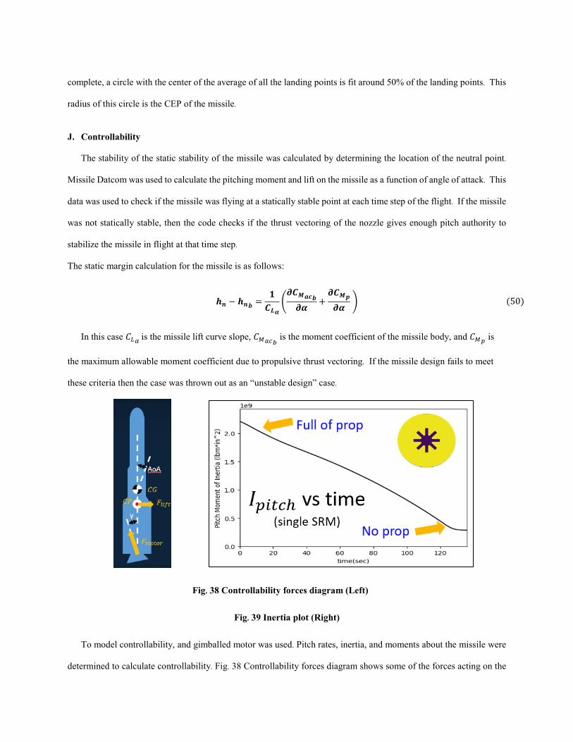
complete, a circle with the center of the average of all the landing points is fit around 50% of the landing points. This

radius of this circle is the CEP of the missile.

J. Controllability

The stability of the static stability of the missile was calculated by determining the location of the neutral point.

Missile Datcom was used to calculate the pitching moment and lift on the missile as a function of angle of attack. This

data was used to check if the missile was flying at a statically stable point at each time step of the flight. If the missile

was not statically stable, then the code checks if the thrust vectoring of the nozzle gives enough pitch authority to

stabilize the missile in flight at that time step.

The static margin calculation for the missile is as follows:

𝒉𝒉𝒊𝒊 − 𝒉𝒉𝒊𝒊𝒃𝒃 =𝟏𝟏𝑻𝑻𝑳𝑳𝜶𝜶

�𝝏𝝏𝑻𝑻𝑴𝑴𝒂𝒂𝒄𝒄𝒃𝒃𝝏𝝏𝜶𝜶

+𝝏𝝏𝑻𝑻𝑴𝑴𝒑𝒑

𝝏𝝏𝜶𝜶 � (50)

In this case 𝐶𝐶𝐿𝐿𝛼𝛼 is the missile lift curve slope, 𝐶𝐶𝑀𝑀𝑚𝑚𝑐𝑐𝑏𝑏 is the moment coefficient of the missile body, and 𝐶𝐶𝑀𝑀𝑝𝑝 is

the maximum allowable moment coefficient due to propulsive thrust vectoring. If the missile design fails to meet

these criteria then the case was thrown out as an “unstable design” case.

Fig. 38 Controllability forces diagram (Left)

Fig. 39 Inertia plot (Right)

To model controllability, and gimballed motor was used. Pitch rates, inertia, and moments about the missile were

determined to calculate controllability. Fig. 38 Controllability forces diagram shows some of the forces acting on the

missile. The inertia of the entire rocket had to be modeled per stage and then the inertia of the entire rocket was

calculated. Then the Center of Gravity was determined. The max change in pitch rate could be determined from the

maximum moment and inertia values. Moments come from both the gimballed thrust and the lift from the AOA.

To determine the moment of inertia, each missile stage was discretized into individual, time-dependent elements.

These elements are constituted by solid rocket motor mass components, interstages, and payload masses. All masses,

with exception to that of the propellant, casing, and insulation are assumed to be point masses. The propellant, casing

and insulation masses are assumed to be one-dimensional distributed masses. It is assumed that, throughout the

operation of the solid rocket motor, the mass distribution of the propellant remains equivalent along the bore is reduced

by the amount of propellant consumed. This is the case for any standard grain configuration that burns from a common

bore. For a wired end-burning configuration, the propellant is assumed to be initially exhausted from the aft end and

progresses towards the head-end throughout the burn.

When the code was setup the first iteration optimized on the thetas, or missile pitch angles. This did not lend well

for determining controllability since the next theta maximum or minimum would need to be determined from many

theta values before it. This is shown in Fig. 40. Right at the beginning the missile tended to always have an extreme

pitch rate that was unobtainable. This is labeled as the angle in the plot for pitch angle. The flight path angle was

labeled as theta. Additionally, Alpha-Q would be way too high at this point and the rocket would break. The next

attempt was optimizing on gimbal angles. This was to try to model controllability from the source, however, this was

very difficult to optimize on because of the alpha-Q constraint causing the optimizer to avoid exploring areas of

interest. Multiple quick changes in gimbal angle may allow for an acceptable max alpha-Q, however this can be

difficult to determine because it required multiple variables to be simultaneously be tested. Lastly, pitch rate

optimization was modeled. This allowed a maximum pitch rate. While there may be extreme cases where a pitch rate

may not be achievable in the middle of boost, after the constraints on the beginning, any pitch rate that might be

required was determined and assumed to be achievable.

Fig. 40: Pitch Angle Optimization before Controllability Constraint

Fig. 42 shows the graph of the boost trajectory once the controllability constraint and alpha-Q constraints are

added. Before the trajectory code is run, the max pitch rates are determined. These are then optimized on using and

optimizer coupled with the trajectory code. A certain number of pitch rates were optimized on, to ensure max range,

while avoiding too high of a runtime. There were about 25 pitch rates numbers that were optimized on during the boost

phase. Since the first section of boost is in the atmosphere and thus more sensitive, more of the pitch rates were

optimized on this first section. The maximum rates were set to an extreme of 1.5 degrees/sec, however, most optimized

pitch rates were less than 0.5 and very few vehicles had any pitch rates higher than 1. The Saturn V had maximum

pitch rates around 0.5 degrees/sec [27]. The first few pitch rates are always optimized to be the highest. A constraint

was then applied to ensure controllability. Based on the max achievable change in pitch rate the first couple of pitch

rates were constrained with the first being 0. And then numbers following being a number between 0 and 1.5

degrees/sec this was constrained until the max pith rate could optimize on 1.5 degree/sec. Then all following max pitch

rates could be 1.5 degrees/sec.

The max change in pitch rate was determined from the moment and the Inertia of the rocket. Since the critical

change in pitch rate was assumed to be right at the beginning of flight then the inertia was only calculated at that time.

Thrust was also calculated at that time. The max gimbal angle was assumed to be 10 degrees. Then the moment was

assumed from the calculated center of mass. The change in pitch rate (angular acceleration - α) was determined from

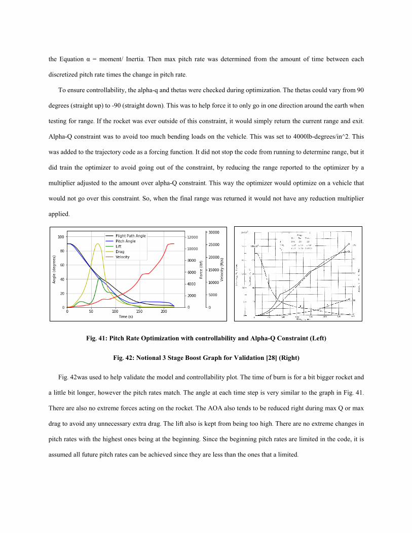
the Equation α = moment/ Inertia. Then max pitch rate was determined from the amount of time between each

discretized pitch rate times the change in pitch rate.

To ensure controllability, the alpha-q and thetas were checked during optimization. The thetas could vary from 90

degrees (straight up) to -90 (straight down). This was to help force it to only go in one direction around the earth when

testing for range. If the rocket was ever outside of this constraint, it would simply return the current range and exit.

Alpha-Q constraint was to avoid too much bending loads on the vehicle. This was set to 4000lb-degrees/in^2. This

was added to the trajectory code as a forcing function. It did not stop the code from running to determine range, but it

did train the optimizer to avoid going out of the constraint, by reducing the range reported to the optimizer by a

multiplier adjusted to the amount over alpha-Q constraint. This way the optimizer would optimize on a vehicle that

would not go over this constraint. So, when the final range was returned it would not have any reduction multiplier

applied.

Fig. 41: Pitch Rate Optimization with controllability and Alpha-Q Constraint (Left)

Fig. 42: Notional 3 Stage Boost Graph for Validation [28] (Right)

Fig. 42was used to help validate the model and controllability plot. The time of burn is for a bit bigger rocket and

a little bit longer, however the pitch rates match. The angle at each time step is very similar to the graph in Fig. 41.

There are also no extreme forces acting on the rocket. The AOA also tends to be reduced right during max Q or max

drag to avoid any unnecessary extra drag. The lift also is kept from being too high. There are no extreme changes in

pitch rates with the highest ones being at the beginning. Since the beginning pitch rates are limited in the code, it is

assumed all future pitch rates can be achieved since they are less than the ones that a limited.

K. Cost Modeling

To justify the ranking of the selected missile systems, it was necessary to determine their production costs. These

costs are representative of not only the missile production cost, but also that of the research and development (R&D)

program, the operational and maintenance costs, and the costs of any necessary upgrades or acquisition of missile

launch infrastructure. For the SLIMJIM cost estimations, it was assumed that regressions based on tactical missile

were sufficiently representative of general trends. However, to take into consideration the difference in tactical and

strategic architectures and associated costs, semi-empirical were utilized to modify the relationships found in the

literature. Modeling the cost of research and development was accomplished with the following equation where 𝑡𝑡𝑅𝑅&𝐷𝐷

is the time of the research and development period in years and 𝛼𝛼𝑐𝑐𝑡𝑡𝑝𝑝𝑚𝑚 is representative of the multiplier to allow the

regression to be used for a strategic system:

𝑻𝑻𝑹𝑹&𝑫𝑫 = $𝟐𝟐𝟓𝟓.𝟗𝟗𝑬𝑬𝟔𝟔 ∗ 𝜶𝜶𝒄𝒄𝒐𝒐𝒊𝒊𝒕𝒕(𝒕𝒕𝑹𝑹&𝑫𝑫)𝟐𝟐.𝟎𝟎𝟐𝟐 (51)

The next cost that was modeled was the cost of the 1000th missile system. This regression exists as an

approximation of the steady-state production cost for a single unit. That is, it is assumed that the learning curve on

manufacturability no longer allows any significant reduction in subsequent systems.

𝑻𝑻𝟏𝟏𝟎𝟎𝟎𝟎𝟎𝟎 = $𝟏𝟏𝟏𝟏.𝟏𝟏𝟔𝟔 ∗ 𝜷𝜷𝒄𝒄𝒐𝒐𝒊𝒊𝒕𝒕�𝑾𝑾𝒑𝒑𝒐𝒐𝒐𝒐𝒊𝒊𝒅𝒅𝒊𝒊�𝟎𝟎.𝟏𝟏𝟗𝟗𝟔𝟔 (52)

Here, 𝑊𝑊𝑝𝑝𝑡𝑡𝑠𝑠𝑝𝑝𝑐𝑐𝑝𝑝 is the weight of the missile in pounds and 𝛽𝛽𝑐𝑐𝑡𝑡𝑝𝑝𝑚𝑚 is a tactical-strategic modifying coefficient. The

final regression was that of the cost necessary to upgrade a missile silo to accommodate the SLIMJIM system.

𝑻𝑻𝒊𝒊𝒊𝒊𝒑𝒑𝒐𝒐 = $𝟑𝟑𝟏𝟏.𝟎𝟎𝑬𝑬𝟔𝟔 ∗ 𝜸𝜸𝒄𝒄𝒐𝒐𝒊𝒊𝒕𝒕 (53)

Where the cost is per silo and 𝛾𝛾𝑝𝑝𝑖𝑖𝑤𝑤𝑡𝑡 represents the extent of the upgrade. The last necessary relation to describe is that

of the learning curve modification of missile acquisition cost. As mentioned previously, the cost of acquiring

subsequent missiles decreases with an increase in manufacturing knowledge. To determine the cost of each system, a

learning curve law is utilized where 𝐶𝐶𝑚𝑚 is the cost of the xth missile, 𝐶𝐶1 is the cost of the first missile, and L is a learning

curve whose value is between 0 and 1.

𝑻𝑻𝟕𝟕 = 𝑻𝑻𝟏𝟏 ∗ 𝑳𝑳𝐥𝐥𝐜𝐜𝐥𝐥𝟐𝟐 𝟕𝟕 (54)

VIII. Design of Experiments

A. Design of Experiments and Approach

When considering how to test a new design there were a couple of different options. These are shown in Table 13:

Experimental options. The first would be to iterate to the ideal missile. This takes an existing design and attempts to

iterate on it to reach a better solution given the new constraint. However, this may miss exploring some of the design

space and options. The next would be to optimize on all the variables. This may explore the entire design space,

however, because the problem is so complex, there is no guarantee of convergence, and a lot of time could be spent

developing a program that eventually does not work in time or at all. Lastly there is the design of experiments method.

This method simply tests as many types of missiles in the design space. It uses a space filling design to try to capture

random variable combinations over the entire design space. Then statistical analysis can be run to best determine the

optimum categorical variables and eventually the continuous variables. While it does not test every single combination

in a full factorial, it tests enough to make generalizations about what works well and doesn’t and helps to refine the

ranges of variables being tested to get the best overall result in the end.

Table 13: Experimental options

Method Description Pro Con Selection

Iteration to Ideal

Start with baseline missile; iterate on variables to reach optimum

Simple to scheme

Does not sample entire design space

No – entire design range not explored – could converge on inferior missile

Optimization of Variables

Optimize variables over design range

Sampling of entire design space

No guarantee of convergence

No – convergence can be an issue and no guarantee of global optimization

Design of Experiments

Intelligently select combinations of variables in design range – converge to optimum

Sampling of entire design space

Sparseness of design difficult to predict

Yes – allows for good exploration of space with combination of experimental schemes

The basic method of how the DOE was run is shown in Fig. 43. The first thing that was done was defining all the

options in the design. These are the continuous and categorical variables shown in Table 14 and Table 15. Then the

DOE has to be setup to test all the different combinations then analyzed using a modeling and simulation environment

shown in Fig. 43 Design flowchart. The design space is then analyzed and the maximum and minimums of the variables

are increased or decreased to improve the cases in the next run. This is done until there are enough missiles shown

that meet the criteria. A Pareto frontier is expected to show up in which there are optimal solutions that are the

maximum range for a given weight. Next, a very high fidelity run that takes a lot longer on the missiles close to the

criteria on the Pareto frontier is executed. Finally, 4 missiles are down-selected and a final decision is made. This

missile is then double checked and analyzed to determine its exact capabilities and to get plots and diagrams of every

part of the missile.

Fig. 43 Design flowchart

A subset diagram of a single iteration is shown in Fig. 44 Testing framework. This DOE is run many times to down

select and improve the design. There are two major types of variables: categorical and continuous. This is separated

because every combination of categorical variables needs to be tested separately in order to determine the best

combination since some categorical variable options may work better by themselves, but worse if coupled with other

certain options. Therefore, the combinations have to be looked at as a whole. On the other hand, the continuous

variables can use a space filling design. So, for every combination of categorical variables there is a space filling

design to test all the continuous variables. A latin hypercube was used. Once categorical variables are decided, the

continuous ones can be run in much higher numbers for that category so a decision can be made on those. Additionally,

as each test is run, extremes values that cause case failures or very undesirable missiles for one continuous variable

can be identified and cut out on each sequential run. There were about 10 different iterations on the code base design

until the final missile was decided upon. Many of these iterations were to add a new factor into the design.

Fig. 44 Testing framework

B. Design of Experiments Setup, Categorical and Continuous Variables

To run the Design of experiments a range of variables had to be determined. Many of these were determined by

constraints of the missile, historical data, and some experience from team members. The boost length was the

allocation of the boost section minus the nozzle length and the top stage length. There was assumed a length of 15ft

for the top section and 5-10ft for nozzle lengths. So, the max length was set at 55 and the minimum was set at 30. At

first, 5 ft discretization was tested, although later this switched to 3 ft. The next was Stage diameter, the maximum

was 10 based on a 12ft silo and the minimum was 4 based on the payload diameters. At the start there was a 2 ft

resolution, however this ended up going down to a 0.5 ft resolution and the maximum reduced to 8ft for stage 1 and

different lower maximums for upper stages, since these returned way too heavy rockets. Length was modeled as a

percentage of the boost length. So, for the number of stages there could be a different percentage that added up to

100% of the boost length. The grain ID was the inner diameter of the grain based on a percentage of the stage diameter.

So, a 50% inner grain diameter of and 8ft diameter section was 4ft. the Grain OD was a percentage of the grain ID.

This was applicable for finocyl and star types of grains which have the lowest point as the grain ID and the tip of the

star or the finocyl grain being the grain OD. This was setup so it could not exceed the diameter of the stage. This

variable was later opened up so there could be maximum grain ODs up to 300% of the grain ID. The grain IDs could

eventually be tested as low as 10% of the stage diameter. The resolution on all of these was refined as more constraints

were placed to avoid failed cases. Number of fins, while discrete, was treated as a continuous variable. Lastly Fin

width was tested, when running the design of experiments this was determined to not effect design much at all so it

was eventually just set to 5%.

Table 14: Continuous variables

Table 15 shows some the different categorical variables that were tested. The biggest variable was the number of

stages. The code had to be designed to be able to test different number of stages. The other major variables was the

grain geometry type or either finocyl or star configuration. Bates grain was not considered due to the poor performance

nature. Lastly the different propellant types were considered. After running the design of experiments for a couple

iterations, theses variables were down-selected.

Table 15: Categorical variables

The design of experiments was then setup using a space filling design. A full factorial with discretized continuous

variables could take trillions of runs; however, a space filling design just tests enough runs to get information back

about the best options. A few hundred runs were able to determine what was causing failed cases, while a few thousand

runs were required to start making decisions. At the beginning of the simulation all the combinations were determined

and then a subset were chosen at random to be tested.

Parameter Min Max Start Resolution Boost Length (ft) 30 55 5

Stage Diameter (ft) 4 10 2 Stage Length (% boost) 20 40-60 5

Grain ID (% Stage Diameter) 20 50 15 Grain OD (% Grain ID) 125 150 25

Fin Width (% Stage Diameter) 2 8 3

Number of Fins 4 8 2

Parameter Options Solid Rocket Stages 2 3 4

Grain Geometry Type Finocyl Star

Propellant (solid fuel) TP-H-1202 TP-H-3340 TP-H-1148

C. Modeling and Simulation Environment

Fig. 45 shows a diagram of the modeling and simulation environment. This was the environment in which the

missiles were tested in a multidisciplinary environment. This diagram takes in all the different parts of the technical

approach to run and test the entire missile. Most everything was able to be tested in line, with an exception of a few.

These few being, CBAERO for TPS weight sizing, post boost propulsion, and glide vehicle range determination code.

Propulsion, geometry, weights, aerodynamics, and trajectory were all able to be run together. TPS weight was

determined on a notional trajectory for a given range and then was set as the weight for part of the payload during

future iterations. Glide vehicle code simply determined the maximum extra range based on a notional trajectory at a

given range. This was then interpolated to determine the maximum range by adding the interpolated glide range to the

range without gliding. Three different glide trajectories were created, one for a total range of 3000 nmi, 6000 nmi,

and 9000 nmi. The TPS thickness and weight for each of these three trajectories was determined and the maximum

TPS weight between the three trajectories was selected. Using the glide distance for each of those trajectories, the

glide range for intermediate ranges was determined with interpolation.

Fig. 45 Modeling and simulation environment

There were many parts of the modeling and simulation environment that were able to be run in line. The code first

set up a list of thousands of different missiles to test. Then missiles were run at random. Each missile contained a set

of variables that was fed into the run manager. After the DOE variables were fed into the run manager of the simulation

the variables would be unpacked and setup to run the propulsion code first. The variables just define the geometry for

some major individual sections of the rocket, but overall geometry determined the exact geometry for the entire rocket.

Then the propulsion code would feed the geometry variables that are calculated for the SRM back into geometry.

Geometry code would then test to make sure these variables would fit within size constraints and resize if necessary

or throw out the case if it couldn’t resize it. Then geometry would calculate the weights of all the parts based on

regression equations for some and use analytical equations for other weights. Geometry should now have the overall

weight vehicle and the exact sizes; these were then fed into aerodynamics to determine the CD and CL values at

different Mach, AOA, and altitude. Then trajectory was run, trajectory optimized on the max range given all the

parameters. Post boost propulsion, glide code, and TPS would be run separately to determine the exact weight of the

post boost section for re-entry. The range was very sensitive to the weight of the post boost section so it was critical

these weights were accurate. Lastly a plot would be able to be created with the main factors being range and weight.

It was then easy to compare the different categorical variables, and make a decision on those. The continuous variables

could also be converged on as well. For the final selection, continuous variables were chosen as options on a pareto

optimum frontier, when the only options left resided in one category.

D. Iterations of the DOE

When running the design of experiments there were many iterations on the code, as time allowed more factors to

be taken into account and new factors came to light. There were about 10 iterations of rockets each one either fixing

a problem, refining the design, or adding new factors onto the design. Fig. 46 First DOE iterationshows the very first

run of the DOE. There were only about a thousand runs, however this helped improve or initial guesses on ranges a

lot and fix some issues. This section will go over some of the major changes between iterations.

Fig. 46 First DOE iteration

Some of the first things taken into account were cases that caused failures. Many failures were caused simply

because the missile could not get off the ground. Some checks were made when the missile was put together to ensure

the missile was not too top heavy and there was a reasonable grain geometry in the first stage to provide sufficient

thrust. Essentially, these were decided by looking at the failed vs. successful cases and seeing which variable ranges

always caused success of failure. Then cutting out the ranges that always caused failure. Additionally, easy volume

checks on the whole missile were added to ensure the weight was at least within a reasonable range to get the necessary

distance. It was also discovered the first run did not model past half earth so that was fixed, however,a new source of

error was found. Some of the runs were simply orbiting. This was found out in Fig. 47, when the height was plotted

for cases that were timing out. Therefore, a max range was set at one orbit of the earth.

Fig. 47 Height (ft) of orbiting missile

When the code was first set up, it had the ability to run the propulsion code which gave basic weights and thrust

curves, missile datcom, and pitch angle optimization trajectory code. Some of the other factors were added as the code

progressed. One was the weight regressions, this included all the interstages, avionics, wiring, and fairings weight.

Another factor that was improved on was weight estimation during flight. Originally it was just linear for each stage;

however, later it became directly estimated from how much mass was expelled at different times of the thrust profile.

Between each iteration the code was improved to get the most accurate result in the least amount of time. Since the

accuracy relies on the discretization of timesteps and has to optimize of a certain number of pitch rates or angles, it

was important to find a sweet spot that didn’t take forever but would still yield results within 100nmi. Better ways to

save more data about the missile for analysis was also added between iterations. This way once at the last iteration, all

the necessary information would be present to make informed decisions quickly. This included both raw number data

and plots showing the missiles to ensure they were flying as expected. The final factor that was added to the code was

controllability constraints and pitch rate optimizations.

One of the other big additions wasn’t really a new factor but a way to run the code fast enough to get enough data

to run statistical analysis and explore the entire design space. There was a cluster of computers available, however

they were linux and one program, missile datcom, was only designed to be run on windows. So, a surrogate model

had to be created in order to run many runs very quickly. Parallel processing also had to be devised and added to fully

use all the cores available on a computer. The first cluster run shown in Fig. 48 was able to produce 95,000 runs. It

was ~20 times faster than running on a single 8 processor computer. This was because the cluster had multiple

computers available to run on, each with 24 processors per computer. Before it took multiple days to get enough runs

to analyze on the first iterations, now only took about half a day. This also meant higher fidelity runs could be run

right at the beginning. Higher fidelity typically meant that the range would increase sometimes by up to 1000nmi due

to improved timestep intervals. The only downside being that the surrogate model did not fit very well. So, the final

cases may vary by +/- 500nmi. This meant that the most promising runs from the pareto frontier had to be selected

and rerun on the slower computer.

Fig. 48 Cluster run

Fig. 48 shows all the first cluster runs. Since, the final weight of the post boost stage was not available at the time,

multiple post boost weights were tested. This was because the midcourse, glide vehicle, and TPS weight were not yet

decided on or figured out yet. When analyzing different cases in the results, the categories were only looked at with

one post boost weight. There were some interesting effects noticed when analyzing the data overall. The Pareto

optimum frontier is shown for the lower post boost weight runs in red. Before for lower ranges this line remains mostly

linear, until the vehicle starts to hit the half earth mark. Then the pareto starts curving upward until it hits half earth

mark. At that point many of the cases go to orbital, and there is not really any more difference in weight to encircle

the earth. Of course, the vehicle can also just go around in the opposite direction at that point. Lastly, and effect also

noticed was a grouping of runs right after they broke the half earth length. This effect reason is unknown. However,

these are cases past objective so they can probably just be considered as sufficient to reach objective. Same as orbital

cases.

Half Earth

Orbital

Lower Post Boost Weight

Higher Post boost Weight

Failed Cases

Pare

to F

ront

ier

The last big iteration on the DOE was to add the controllability constraint. This was more difficult to model so it

was not added until right up at the end

IX. Results

A. Model Fit and Verification

After compiling the data from the design of experiments, the next step was to create surrogate models to predict

the results for any combination of the rocket architecture that was not tested in the DOE. Using surrogate models is

advantageous because the response can be determined in seconds, while running the architecture through the virtual

trajectory environment takes much longer to determine weight and range. Neural nets were used for the surrogate

models to predict the range and weight of a given rocket configuration as a function of grain type, length and diameter

of each stage, as well as the grain geometry. The surrogate model for the range had an 𝑅𝑅2 value of 0.91, while the

model for the weight was 0.99. In Fig. 49 the prediction profiler for the range and weight are shown with the

independent variables used. In the figure, it is clear to see how the responses are expected to change as the each of the

independent variables vary.

Fig. 49 Prediction Profiler

Additional ways to view a goodness of fit include inspecting the Actual vs Residual plots, which can be seen

below. An Actual vs Residual plot shows a good fit if the points are very random and there is no obvious pattern.

Fig. 50: Residual Plot of Fit (Left)

Fig. 51: Categorical Variables Prediction Profiler (Right)

The purpose of using the surrogates was to determine the combination of the categorical variables that would result

in the highest range. However, the residual plot shows a varying range of 1500nmi between the predicted and the

actual, so the model for the range was not a good predictor. Therefore, an alternative method was used to determine

the optimal categorical variables that involved finding combinations along the Pareto frontier of the weight vs range

plot.

B. Categorical variable Selection

Determination of the categorical variable selection as specified in Table 16 was accomplished by utilizing a design

of experiments scheme that varied both the categorical variables and continuous variables. Specifically, the categorical

variables were ran as a full-factorial combination and the continuous variables were sampled using a modified Latin

hypercube design. The goal of this methodology was twofold: to determine relative variable sensitivities, and to

determine an optimal combination of categorical variables.

In the initial set of runs to reach this goal, the simulation environment was queried with 37,000 missile designs.

These initial runs showed that key metrics such as missile weight and range are insensitive to the continuous variable

thickness of fin ports in Finocyl-style propellant grains. This allowed for a moderate collapse in design space by

keeping that variable constant at 5% of grain diameter. The second immediate takeaway from this set of runs was the

determination of the optimal number of stages for the missile. The number of stages that produced the most cases

falling along the pareto frontier was chosen. Fig. 52 shows that the 3-stage configuration is generally superior in terms

of longer range and lower weight than 2 and 4 stage missiles.

Ran

ge

Wei

ght

Fig. 52 - 3 Stage Categorical Justification

The final steps in the selection of categorical variable were to determine the propellant and grain type to be used

in each stage of the missile. To accomplish this, various combinations of these variables were plotted on similar weight

versus range graphs and examined for closeness to the pareto-optimal frontier. It was shown that the use of the

propellant TP-H-1202 was the superior propellant for each stage. This is consistent with this propellant’s properties

as it has a moderately high chamber temperature corresponding to a high specific impulse. Fixing this propellant

choice, several combinations of possible grain geometries were explored, shown in Fig. 53. Of these, the combination

closest to the pareto frontier was chosen. Fig. 54 shows an analytical representation of the same categorical

combination were the cost function of interest (maximization of range and minimization of weight) is highest.

Fig. 53: Categorical Range vs Weight Plots

Fig. 54 Model Fit to determine optimum categorical Combinations

Table 16 shows the final variable selection, where it is shown that all three stages should utilize a Finocyl grain

geometry. It should be noted that another configuration nearly equivalent to the selected optimum (shown as the right-

Weight

Range

most peak in Fig. 54) utilized a star grain for the 3rd stage. Using a Finocyl grain, however, was chosen to simplify the

manufacturing of the grains and mandrel.

Table 16 Final Categorical Variables

C. Continuous Variable Options

Fig. 55 is a plot of the final cluster runs once the categorical variable were down selected. There were about 50,000

cases in the final run. However, these were still off by about +/- 500nmi because of the missile datcom surrogate

model. Therefore, the cases had to be run again. About 100 of the best cases were taken from the pareto frontier and

rerun with the higher fidelity code. The selected cases are circled. The final returned values are then used to help down

select four missiles for the final selection and to decide on what the continuous variables should be. All of these

missiles take into account controllability, missile maximum size, TPS, and the other containing factors. They do not

take into account glide range, that is added later separately. They only have the throw range which is the range with

no glide, and 0 lift is assumed for a ballistic re-entry.

Fig. 55: Final DOE Iteration: Cluster Runs

Fig. 56 shows the cases after they have been rerun at a higher fidelity. Four missiles were then selected on the

pareto frontier that were able to meet either threshold or objective. The plot also shows a relatively linear pareto

frontier when the final cases are run. Missile 1,2,3,4 are circled in blue on the pareto frontier and are further analyzed

in the results section of the report.

Fig. 56: Final DOE iteration; selected high fidelity runs

Table 17 shows all the basic parameters returned from running the code. This does not include glide range, which

is added later.

Table 17: Missile Options without glide range

Missile Throw Range (nmi) Weight (lbm) Length (ft) Max Diameter

(ft) Time (s)

1 6,100 102,000 70 5.5 34.7 2 6,800 108,000 68 6 38.7 3 7,300 110,000 68 6.5 37.4 4 9,300 122,000 69 6.5 46.7

Missile options with the additional glide range are shown in the Table 18. These are discussed more in detail the

glide results section.

Table 18: Missile Options with glide range

Missile Throw Range (nmi)

Throw Time (min)

Additional Glide Range

(nmi)

Additional Glide Time

(min)

Total Range (nmi)

Total Time (min)

1 6,100 34.7 970 19.4 7,070 54.1

2 6,800 38.7 1060 20.9 7,860 59.6

3 7,300 37.4 1130 21.9 8,430 59.3

4 9,300 46.7 1380 25.9 10,680 72.6

Fig. 57 shows CAD drawings of each of the 4 missiles to scale. It can be seen how the missile increases in size

with increase range. These are all to scale.

Fig. 57 Missile CAD drawings

D. Thermal Protection System Sizing

As seen in the table summarizing the performance characteristics for each of the four missiles above, the maximum

distance the reentry vehicle glides changes from 970 nmi to 1340 nmi. As a result, the reentry vehicle is exposed to

different aerothermal conditions. This means the TPS will be different for the different reentry vehicle trajectories.

However, in order to properly size the TPS, the minimum trajectory also needs to be considered to ensure the TPS can

handle any trajectory the missile may have. The minimum range for the SLIMJIM was set to be 3000 nmi since

anything less is considered an Intermediate Range Ballistic Missile (IRBM), and the intention was to have no gaps in

Missile 1

Missile 2

Missile 3

Missile 4

the capabilities between the IRBM and the ICBM. Therefore a 3000 nmi range trajectory was also considered for each

missile to see how the TPS compared to the maximum range TPS. The table below shows the maximum heat rates

and the maximum temperatures for each of the four trajectories, as well as for the minimum 3000 nmi range.

Table 19 Maximum Heat Rate and Temperature of RVs

Missile Trajectory Maximum Temperature (Rankine-Kelvin)

Maximum Heat Rate (Btu/sft2-W/cm2)

Minimum Range Trajectory (3000 nmi) 6740.8-3744.9 785.5-892.1

Missile 1 Max Range 7084.3-3935.7 958.3-1088.3

Missile 2 Max Range 7083.18-3935.1 957.8-1087.7

Missile 3 Max Range 7082.46-3934.7 957.3-1087.23

Missile 4 Max Range 7079.4-3933.0 955.6-1085.3

As seen in the table above, the maximum temperature for all the trajectories is about 7080 Rankine, and the heat

rates are also similar at about 957 Btu/sft2. This maximum temperature is above the maximum material limit for RCC,

which was 2959.2 degrees Rankine, leaving the PICA and the Carbon Phenolic as the only suitable candidates for the

TPS material. In order to determine which material to use, the thickness and weight was determined for each material

using the trajectory for missile 4. After determining the overall thickness and weight of a Carbon Phenolic TPS using

the longest-range trajectory, it was found the thickness needed to be 9.25 in., weighing 1545 lbm. The PICA TPS of

the same trajectory resulted in a thickness of 3.51 in., and only weighing 142 lbm. Although Carbon Phenolic can

reach much higher temperatures than PICA, the PICA was selected as the TPS material because it is significantly less

dense and requires a lower thickness, resulting in a significantly lower weight. Using PICA as the TPS material, the

weight and thickness was determined for each of the maximum range trajectories and the minimum range as well.

These results can be seen in the table below.

Table 20 TPS Sizing for each Trajectory

Missile Trajectory Range (nmi)

Material Required for

Insulation (in)

Material Required for

Recession (in)

Overall Thickness

(in) Weight (lbm)

Minimum Range Trajectory (3000 nmi) 3000 1.57 0.39 1.96 79

Missile 1 Max Range 7,070 2.28 0.72 3.0 121

Missile 2 Max Range 7,860 2.31 0.80 3.11 126

Missile 3 Max Range 8,430 2.34 0.85 3.19 129

Missile 4 Max Range 10,680 2.44 1.07 3.51 142

According to the table above, the required material for both the insulation and the recession increases as the range

increases. This is expected because a longer range means the reentry vehicle glides for longer. Even though the reentry

vehicle in each trajectory experienced similar maximum heating rates, a longer trajectory must have a TPS that can

withstand the higher heat load due to prolonged exposure to heating. Therefore, as the missile range increases, the

weight of the payload also increases since the TPS weight increases. This trend will need to be considered when

selecting the final missile architecture since a heavier payload will result in a more expensive missile system.

E. CEP Results

The CEP Results for the four candidate missiles are presented in the following table. All the CEP values were

determined from a distribution of 1000 landing points for each missile. 1000 points is enough to characterize the CEP

of the missiles for the trajectory simulation, because after 200 trajectory simulations, the change in CEP became

negligible with an increase in the number of runs.

Table 21: CEP Results

Missile 1 CEP Missile 2 CEP Missile 3 CEP Missile 4 CEP

57 ft. 49 ft. 61 ft. 53 ft.

All the missile CEP values are around the same order of magnitude, so CEP played a minor factor in the down-

selection of the missiles, but the values do confirm that all the candidate missiles meet the objective CEP requirement

of 100 ft.

Because there are no notable differences in the distribution of the landing points of the four missiles, it is not

necessary to show all the missile landing point distributions. The landing point distribution of the chosen missile,

missile 1, is shown in the figure below.

Fig. 58 Chosen Missile CEP

F. Midcourse Results

Midcourse correction simulations were created to estimate the amount of fuel required in post-boost solid rocket

motors (PBSRM) to maneuver and achieve a footprint of 100 nmi. These were done using trajectories for threshold

and objective missiles. The PBSRM weight estimated for a objective missile was 280 lb each for a total added weight

of 560 lb. Threshold missiles would require approximately 470 lb added weight total.

Table 22 Midcourse results

Objective Threshold

PBSRM Weight 280lb each = 560 lb 235lb each = 470 lb

G. Glide Vehicle Results

An optimization for minimum glide distance, maximum glide distance, and maximum cross range glide range was

run on the reentry vehicle. These tests were limited to a maximum g loading condition, as well as a maximum heat

rate condition. For the maximum cross range capability, it was found that the RV would pitch up and glide further in

order to achieve further distance laterally. In order to maximize the capability for the RV to change direction, giving

the RV a shorter trajectory and allowing it to glide further was determined to be more beneficial, as the RV had limited

capability to shorten its range.

Table 23 shows glide ranges and time. 0 lift was considered to have 0 glide range. The minimum glide range means

the control surface and lift was being applied in the opposite direction causing the vehicle to enter at a steeper angle.

Table 23 Glide Ranges and Time

Notional Throw Range (nmi)

Max Glide Range (nmi) Minimum glide (nmi) Glide time (min)

3000 622 -63 13.6 6000 980 -81 18.4 9000 1428 -48 25.7

Fig. 59 and Fig. 60 show the interpolations of glide range and time. Using three points it is shown that these

functions are linear and can be interpolated as such.

Fig. 59 Glide Range vs. Throw Range (Left)

Fig. 60 Glide Time vs Glide Range (Right)

To compare the performance of different glide vehicles, the glide capability and aerothermal response for each

different reentry vehicle configuration was analyzed using the same trajectory, which had a total range of 7000 nmi.

The table below displays the different glide ranges for each of the reentry vehicle geometries considered.

Table 24 Glide range for different RV shapes with a throw range of 7000 nmi

706 nmi 1341 nmi 1579 nmi 1608 nmi 1724 nmi

From the results in the table above, it is clear that the maximum range of the vehicle increases as the wing span

increases, which can be expected. However, the aerothermal analysis is still needed to see how the change in wingspan

affects the heating of the reentry vehicle.

When designing the reentry vehicle, different size control surfaces were examined to find the best vehicle that

could not only maximize glide, but could also fit within the shroud of the missile. However, as the wings increased in

size, the aerothermal conditions at the wings increased as well. The image below show the maximum heat rate for

reentry vehicles with varying wingspan for a given trajectory.

Fig. 61 Heat Rate Maps for Various Reentry Vehicle Designs

As the wingspan increases, the heat rate increases as well. For a reentry vehicle with an ablative TPS, this means

more material will be lost. As a result, the control surface degrades more. Increasing the wingspan may increase the

glide capability, but it introduces more uncertainty throughout the flight since the material can vaporize in an

unpredictable manner on the wings, potentially making it harder to control. Additionally, as the glide range increases,

the TPS will have to endure a higher heat load, requiring a thicker material. Therefore not only is more material

needed, but more material will be lost during ablation.

The reentry vehicle selected is shown in Fig. 62. Ultimately a wingspan of 30 inches (or 4 inch wing length) was

chosen as it gave more than enough glide range, and were able to fit within the fairing limitations. Additionally, the

aerothermal response for this geometry was less severe than the other reentry vehicles with a higher wingspan, but

still provided almost twice as much range as the reentry vehicle with the smallest wings.

Fig. 62: Selected RV (1341 nmi glide)

For Cross Range, a bank angle was applied to the 7000 nmi range reentry trajectory. At maximum bank the cross

range could get to 1160nmi (580nmi lateral range each), but sacrifices a lot of downrange capability. The maximum

downrange for this trajectory was 1300nmi, but at the maximum cross range it is only 620nmi downrange.

Interpolating these numbers for a 50nmi cross range gives a 1240nmi downrange. This is about 96.4% reduction in

downrange to achieve the necessary cross range. Therefore the 96.4% was applied to the down ranges for the other

interpolated missiles glide ranges.

The Final glide ranges are shown in the table below.

Table 25 Missile Total Ranges + Time

Missile Throw Range (nmi)

Throw Time (min)

Additional Glide Range

(nmi)

Additional Glide Time

(min)

Total Range (nmi)

Total Time (min)

1 6,100 34.7 970 19.4 7,070 54.1

2 6,800 38.7 1060 20.9 7,860 59.6

3 7,300 37.4 1130 21.9 8,430 59.3

4 9,300 46.7 1380 25.9 10,680 72.6

H. Midcourse vs glide

One of the large differences between using a midcourse correction and using a glide trajectory is the reentry

trajectory for the reentry vehicle. With the midcourse correction, the reentry vehicle experienced steeper reentry

angles, resulting in a reentry trajectory that only lasted a couple minutes. The glide trajectory had much lower reentry

angles, resulting in a much longer trajectory. For the reentry vehicle gliding 1341 nmi, the duration of the flight was

almost twenty minutes. Because the two trajectories were so different, the aerothermal conditions were vastly different.

The images below display the maximum temperature maps for the reentry vehicle using the midcourse correction for

both the threshold range and the objective range.

Fig. 63 Maximum Temperature Map for Threshold Range Using Midcourse Correction (Left)

Fig. 64 Maximum Temperature Map for Objective Range Using Midcourse Correction (Right)

As seen in the images above, the maximum temperature for the threshold trajectory was 7678 K, which is 13820

Rankine, and the Objective range had temperatures higher than that. As a result, only Carbon Phenolic can be used at

these temperatures for the TPS material since RCC has a maximum temperature of 2959 degrees Rankine and PICA

has a maximum temperature of 7675 degrees Rankine. Based on these results, the TPS would be about 3.85 in. of

Carbon Phenolic for the Objective range, weighing approximately 645 lbm.

However, using the glide capabilities results in the following maximum temperature map for an objective range.

Fig. 65 Maximum Temperature Map for Objective Range Using Glide Reentry

The resulting maximum temperature for the glide reentry was 3933 K, which is 7079.4 degrees Rankine. Due to

the lower temperature, PICA can be used as the TPS material which is advantageous due to its low density. As a result,

the TPS for this reentry consists of 3.51 in. of PICA, weighing only 142 lbm. The table below summarizes the different

TPS that would be needed with the midcourse correction and just relying on the glide.

Table 26 Summary of TPS for Midcourse vs Glide Trajectory

Objective Range Trajectory Method

Max. Temperature (Rankine) TPS Thickness (in) TPS Weight (lbm) Time to

Target (min) Midcourse Correction 13820 3.85 645 2.23

Glide 7079.4 3.51 142 25.9

Besides the glide capability reducing the weight of the TPS, the overall weight of the rocket decreases because

two post boost solid rocket motors (SRMs) weighing 470 lb each are no longer needed. Below is a graph displaying

the Rocket Weight vs Range for the rockets with the post boost SRM along with the rockets that do not have the post

boost SRM. As seen in the figure, the rockets without the SRM generally have a higher range as a rocket of the same

weight that does have the SRM.

Fig. 66 Range vs Weight Plot with and Without Post Boost SRM

Based on the comparison previously discussed between using the midcourse correction and allowing the reentry

vehicle to glide to its target, the final design did not include a midcourse correction but instead relied on the glide

capability of the reentry vehicle. By eliminating the need for the midcourse correction, the weight of the TPS and the

weight of the rocket was able to decrease, resulting in a cheaper missile system. The tradeoff for this method is the

reentry vehicle takes longer to reach its target, leaving it more vulnerable to enemy defense systems. However, this

was not considered as important as the decrease in cost.

I. Missile silo justification

Missile silos were chosen as opposed to mobile launch for multiple reasons. First, the size of the missile with

lengths of above 60 ft., diameters above 6 ft. and weights greater than 100,000 lbm would require large, expensive

mobile launch platforms. Secondly, utilizing a mobile launch configuration would present additional issues such as

the maintainment of the infrastructure for keeping 450 missile in constant motion around a large area of land (railways,

bridges, roads), the additional increase in personell required for a mobile launch capability, and the additional response

time it would take to hault and stabilize a mobile launher, and raise the missile into launch orientation. Lastly, it was

determined that retrofitting existing silos would be cheaper than building or aquiring a fleet of mobile launch vehicles.

With Post Boost SRM Weight

Without Post Boost SRM Weight

J. Final Missile Selection: Objective vs threshold tradeoff

Table 27 Missile Selection Overview

Missile Range (nmi)

Time (min)

CEP (ft)

Weight (lbm)

Length (ft)

Max Diameter

(ft)

Total System

Cost ($B)

Requirement Compliance

Range Time CEP

1 7,070 54.1 57 102,000 70 5.5 68.8 Threshold Objective Objective

2 7,860 59.6 49 108,000 68 6 70.4 Threshold Objective Objective

3 8,430 59.3 61 110,000 68 6.5 71.2 Threshold Objective Objective

4 10,680 72.6 53 122,000 69 6.5 74.1 Objective Objective* Objective

The four missiles in Table 27 are sampled from the Pareto frontier in Fig. 56, which means that these missiles have

the best combination of range and weight. From the four down-selected missiles, the final missile was chosen by

looking at the trade-off between meeting the requirements and the cost of the missile, which is directly proportional

to weight. Because the Missile number four is the only missile in the set that meets the objective range requirement

and because its cost was only determined to be 4%-8% greater than a threshold case, it was chosen as the final missile.

The reason that the increase in cost is justified to achieve the objective range is illustrated in Fig. 67 below. This

figure illustrates locations on the earth that the missile can reach given different ranges represented by the concentric

circles. With the highest range of the remaining three missiles, 8430 nmi, it is impossible to reach some parts of

Australia, Madagascar, and other land mass located in the inner four concentric circles of Fig. 67. This is important

because the missile needs to be applicable to the US for the considerable future. All the threshold range missiles can

hit all current countries with nuclear capabilities; however, there is no telling what may happen many years down the

line. Therefore, the increase in overall weight was justified because it enabled the missile to hit anywhere on the planet,

ensuring the ability to provide strike capability against any possible national security threat.

Fig. 67 Target capability from average MM3 silo location

Also, while the time to target may seem high for missile four, if the glide vehicle is pitched so that the total range is

10,000 the glide time is reduced by more than half resulting in a total time to target of 59.8 min which is still within

the objective requirement and only slightly higher than the other three options.

X. Final Missile

A. Range and Capability of selected Missile

1.) Capability:

Table 28 and Table 29 show the capability of the overall rocket selected as discussed in missile selection. Table

30 shows that this missile is meets all objectives presented in the RFP for Range, Time, and CEP. The time objective

barely is met for a 10,000-range target. While the missile still can go a bit longer for more time. It does meet the time

objective requirement for a 10,000 nmi range target right at 59.8min. This time was the limiting factor to meet all

objectives at the lowest overall cost.

Table 28: Final Missile Parameters Overview

Missile Range (nmi)

Time (min)

CEP (ft)

Weight (lbm)

Length (ft)

Max Diameter

(ft)

455th System cost ($

Million)

Requirement Compliance

Range Time CEP

4 10,680 72.6 53 122,000 69 6.5 Objective* Objective Objective

* Meets objective of 10,000 nmi at 59.8min

Table 29: Final Missile Glide Parameters

Missile Throw Range (nmi)

Throw Time (min)

Additional Glide Range

(nmi)

Additional Glide Time

(min)

Total Range (nmi)

Total Time (min)

4 9,300 46.7 1380 25.9 10,680 72.6

Table 30 Objective vs. Actual

Requirement Objective Actual Value

Range 10,000 nmi 9,300 nmi. (Throw Range)

10,680 nmi. (Total Range)

Time to Target 60 min

46.7 min (Throw Time)

72.6 min (Total Time for 10680 nmi)

59.8 min (1000 nmi Range Time)

Precision (CEP) 100 ft. 53 ft.

2.) Weight and Geometry Breakdown:

Table 31 shows the weight breakdown of post boost section of the final missile. There are no PBSRMs because a

glide vehicle yielded better results and could reach the cross-range requirement. The other numbers were calculated

from the regressions in the structures section and the TPS sizing section.

Table 31: Final Missile Post Boost Weight Breakdown

Mass Allocation # Each Total Payloads 2 1000 2000 PBSRMs 0 0 0

TPS 2 142 284 Cold Gas 2 77 153

Structure mass 1 46 46 Payload control 2 128 255

Fairing 1 83 83 Gas Generator 1 100 100

Avionics 1 110 110 Wiring 1 39 39 Total 3070

RV Weight 1345 2690 Other Weight 380

Table 32 shows all the final broken down geometry parameters and solid rocket motor parameters for the

missile.

Table 32: Final Missile Geometry Parameters

Stage 1 Stage 2 Stage 3 Post Boost Length (ft) 23.0 22.9 13.0 15 ft

Diameter (ft) 6.5 5.5 4.5 4.5

Grain

N/A

Grain (ft) ID: 1.6, OD: 3.2 ID: 0.8, OD: 2.5 ID: 1.3 OD: 2.7 - Grain Type Finocyl Finocyl Finocyl - Propellant TP-H-1202 TP-H-1202 TP-H-1202 -

Weight (lbs) 63,600 43,900 11,742 3,070 (1,345 each RV)

Dry Weight (lbs) 5,270 3,589 1,183 - Max Thrust (lbf) 297,700 254,000 99,900 -

MEOP (psi) 1,000 1,000 1,000 Specific Impulse (sec) 249 284 296

Burn Time (s) 84.6 83.7 52.8 - Nozzle Length (ft) 4.5 7 6 - Nozzle Throat (in) 14.7 12.8 7.9 -

Nozzle Exit Diameter (ft) 4.2 5.5 4.5 - Nozzle Expansion Ratio 11.8 26.6 46.7

3.) Missile Figures

Fig. 68, Fig. 69, Fig. 70, and Fig. 71 show all the different diagrams of the missile. Fig. 68 shows the basic overall

shape of the missile. Fig. 69 shows the exploded view of the missile. Fig. 70 shows the shape of the vehicle with see

through fairings. Lastly, Fig. 71 shows the post boost section. This shows the two re-entry vehicles the structures

holding the together until release, and the cold gas section for each RV. The warm gas generator is contained within

the post boost connecting structure. It is also shown there is no post boost solid rocket motors.

Fig. 68: Missile CAD model

Fig. 69 Missile CAD model Exploded View

Fig. 70 Missile Transparent View

Fig. 71 Post Boost Section

B. Missile Plots

1.) Trajectory Plots

Fig. 72 Thrust Profile (lbf) (Left)

and Fig. 73 show the thrust curve and mass flow of the propellant. The thrust profile shows a desirable thrust

bucket in the first stage. It also has a relatively flat thrust profile on the 3rd stage. 1st and 2nd stages are relatively similar

thrust profiles, with the second stage profile being a bit less. 1st stage burn time is 84.6s, 2nd stage burn time is 83.7s,

and the last stage burn time is 52.8s. The overall burn time is right at 221 sec.

Fig. 72 Thrust Profile (lbf) (Left)

Fig. 73 Missile Mass (lbm) (Right)

Fig. 74 and Fig. 75 show the dynamic pressure and Alpha-Q. The dynamic pressure peaks around 60s. It then

quickly drops as the missile escapes the atmosphere. Alpha -Q constraint was set at 4000 degree-psi. It is shown below

that the constraint is met.

Fig. 74 Dynamic Pressure (psi) (Left)

Fig. 75 Alpha-Q (degrees-psi) (Right)

Fig. 76 and Fig. 77 show the AOA and the Acceleration. In the AOA plot the maximum AOA kept to less then

four until the missile starts escaping the atmosphere. At that point the AOA does not really have any lift to cause the

missile to break. The acceleration plot shows the maximum acceleration. This happened during the 3rd stage and was

usually always at this point for all pareto optimum missiles. The max G’s can be seen from this by dividing it by

32.2ft/s2 gravity constant. The Max G’s are right at 18G’s right at the end of the final burn.

Fig. 76 AOA (degrees) (Left)

Fig. 77 Acceleration (ft/s2) (Right)

Fig. 78 and Fig. 79 show the trajectory plot and the pitch rate plot. The trajectory plot shows the flight path angle,

the height and the velocity of the missile during boost. The different stages can be depicted as well. The pitch rate plot

shows a maximum of about .880 degrees/sec. This was not actually a constraint at that point. It was what the optimizer

optimized on. The constrained pitch rates are right at the beginning as it reaches its max pitch rate. This is because of

the maximum change in pitch rate from gimbal angle and inertia.

Fig. 78: Trajectory plot (Left)

Fig. 79 Pitch Rate Plot (degrees/sec) (Right)

Fig. 80 shows a more detailed trajectory plot with all the aerodynamic forces shown. The flight path angle is

measure of the velocity in the x and y direction. The pitch angle is derived from the pitch rates over time. AOA is the

difference between pitch angle and flight path angle. This plot shows how the alpha-Q constraint forces the AOA to

be very small while in the atmosphere. Angle of attack is also kept low during max dynamic pressure. As the stage

separation occurs, it can also be seen how the drag and lift is reduced substantially.

Fig. 80: Detailed Trajectory plot with Drag, Lift, Pitch & Flight Path Angle, Velocity, and Height

Stage 1

Stage 2

Stage 3

Stage 3

Stage 2

Stage 1

Fig. 81 and Fig. 82 show the overall trajectory as a plot of height over time and a 2D plot with the trajectory around

the earth. Just the throw range is shown in these plots.

Fig. 81 Height (ft) plot vs time (s) (Left)

Fig. 82 2D trajectory plot around earth (ft) (Right)

Fig. 83 shows a detailed close up view of the 2D boost. It shows the point at which the stages separate. stage 1

separates in the middle of the highest pitch rate, while stage 2 and stage 3 have very low pitch rates during separation.

Therefore, interstage between stage 1. And stage 2 will require a more controlled and larger structural analysis and

mass to ensure the missile has a good separation.

Fig. 83 Boost Trajectory

2.) Aerothermodynamic Results and TPS Size

The final missile configuration had a maximum range of 10680 nmi, with the reentry vehicle being able to glide

1380 nmi. As previously stated, the minimum range of the missile is 3000 nmi, therefore the TPS on the RV for the

selected final missile configuration needs to be able to handle the aerothermodynamics of both trajectories. The figures

below display the maximum wall temperature and the maximum heat rate for the maximum range and the minimum

Earth

St. 1 Sep. St. 2 Sep. St. 3 Sep.

EARTH

EARTH

EARTH

range trajectories, respectively. Because the maximum wall temperature was below the maximum allowable

temperature for PICA, PICA was used as the TPS material.

Fig. 84 Maximum Wall Temperatures and Heat Rate for Maximum Range

Fig. 85 Maximum Wall Temperatures and Heat Rate for Minimum Range

The maximum range displayed a higher maximum wall temperature and a higher maximum wall temperature.

Additionally, because the duration of the trajectory for the RV was longer for the maximum range, it required more

TPS material for insulation and experienced more recession in the TPS material than the minimum trajectory. The

table below summarizes the TPS size for the maximum and minimum range. The final TPS was 3.51 in. of PICA,

and this is able to handle both the maximum and minimum trajectory.

Table 33 TPS Summary

Range (nmi)

Max. Temperature (R-K)

Max. Heat Rate (Btu/sft2-W/cm2)

Insulation Material Required (in.)

Material Recession (in.)

Required Thickness (in.)

Weight (lbm)

3000 6740.8-3744.9 785.5-892.1 1.57 0.39 1.96 79

10680 7079.4-3933.0 955.6-1085.3 2.44 1.07 3.51 142

3.) CEP Plot

The plot below shows the distribution of 1000 landing points of the final SLIMJIM missile. The CEP, the radius

of the circle which encompasses 50% of these landing points and is centered at the average of the landing points, is

53 ft., which is well below the objective requirement of 100 ft.

Fig. 86 SLIMJIM CEP

4.) Reentry Plots

The glide capability of the reentry vehicle is shown below in Fig. 87 Glide Capability of the Reentry Vehicle.

With no lift, the reentry vehicle travels about 3000 nmi. However, the maximum glide capability produces and

additional 1380 nmi to the range, for a total of almost 4400 nmi.

53 ft.

Fig. 87 Glide Capability of the Reentry Vehicle

The following image shows how the Mach number and dynamic pressure changes throughout the glide trajectory.

Initially the Mach number is around 25 with the dynamic pressure close to 0, but the the Mach number drastically

decreases about where the dynamic pressure increases. This is expected since as the atmosphere becomes denser, there

is more resistance on the RV.

Fig. 88 Mach Number and Dynamic Pressure During Glide Trajectory

C. Costs and Operations

0

2

4

6

8

10

12

14

0

5

10

15

20

25

30

0.00 104.68 209.36 314.04 418.72 523.40 628.08

Dyan

mic

Pre

ssur

e (B

ar)

Mac

h N

umbe

r

Time (s)

Mach Number and Dynamic Pressure During Glide

Mach Number Dynamic Pressure

Determination of the cost of the final SLIMJIM missile system requires the estimation of the empirical values

discussed in the approach section. The modifiers 𝛼𝛼𝑐𝑐𝑡𝑡𝑝𝑝𝑚𝑚 and 𝛾𝛾𝑐𝑐𝑡𝑡𝑝𝑝𝑚𝑚 affecting the cost of the R&D and that of individual

silo upgrade were assumed to be 5 while 𝛽𝛽𝑐𝑐𝑡𝑡𝑝𝑝𝑚𝑚 , affecting the acquisition cost, was assumed to be 3. It was also assumed

that the learning curve factor L would be a worst-case value of 0.75 for this missile system as the US has not produced

a similar missile in more than two decades.

The RFP requires 450 missiles to be produced with accommodating silos, as well as a test salvo of 5 units. This

was to be developed over a 10-year R&D program. The final cost breakdown is shown in Table 34.

It was assumed that per missile complex (encompassing 45 silos), an accompinement of 10 full-time personell

would be required to maintain launch capabilities. It was assumed tha the yearly salary, benefits, equipment, and

training for these personell would be $100,000 per year.

Table 344 SLIMJIM cost breakdown

Item Cost (Billions of $)

R&D 14.6

Silo Upgrades 7.7

455 Missiles 51.8

Total Capital 74.1

Yearly personell 0.045

XI.Conclusion

In conclusion, the design proposal submitted contains details on the SLIMJIM, which carries two

independently guided reentry vehicles that can reach targets up to 10,680 nmi away with a cross range of 100 nmi. By

taking advantage of their glide capabilities, the reentry vehicles also have a CEP of 53 ft, enabling them to destroy

hardened targets that are shallow underground [29] upon surface detonation. Additionally, the SLIMJIM will reuse

the current Minute Man III silos because that is more economically viable than creating a mobile launch system and

its supporting infrastructure. As requested, the SLIMJIM will be able to last 20 years with little to no maintenance.

This is achieved with non-corrosive materials and solid propellants, which are safe to handle and transport. If the

lifetime of the missile expires or there is a superior missile built, the SLIMJIM missile can be used as a transport

vehicle to deliver payloads to orbit since it has the capability to reach the required altitude. The SLIMJIM is designed

to not only meet the requirements of the customer, but to also ensure the United States maintains its status as a credible

nuclear power.

XII.Appendix

A. Space Shuttle Solid Rocket Booster Validation

Propulsion code was validated using data from Space Shuttle Redesigned/Reusable Solid Rocket Motor (RSRM).

There is large amount of public data available on grain geometry for this rocket and there is known propellant

characterization and weight breakdown. A static hot-fire of the RSRM is shown in Fig. 89. Figures from which the

dimensions of the RSRM grain geometry were photographically determined from is shown in Fig. 90.

Fig. 89 Space Shuttle RSRM Test Firing

Fig. 90 RSRM Cross Sections

The main points for validation were validation is the geometric grain propogation, ballistic analysis, and weight

regressions. The validation simulated the RSRM using the public information shown in Fig. 90. There were a few

assumptions made on the unkown parameters, and then the RSRM was tested using the SLIMJIM propulsion code

modeling tool. Differences were then identified. Fig. 91 and Table 35 show the differences between the SLIMJIM tool

thrust profile and the actual test burn of the RSRM. The curves are relatively similar once a correction factor was

added.

Fig. 91 Plot of Thrust vs. Time between SLIMJIM tool and RSRM results

A correction factor of 93.4% (6.6% less) was added to the ISP to adjust the code to fit the RSRM as best as possible.

All the other variables and differences are shown in the table below. The performance is relatively similar, but the

weight regressions are a bit different. The mass regressions are accurate for large motors, however, it is assumed some

mass went up to be safer after the challenger explosion. The differences are assumed to be because a couple of factors.

One may have been because of a high fineness ratio requiring ballistic element analysis. Another may have been

because it was assumed to be an ideal SRM, therefore did no have thermochemical analysis. The last was because the

actual SRM dimensions are unkown, they were interpreted from pictures that were to scale. The max mass flux of this

motor was 2.2lbm/sec/in2.

Table 35: RSRM vs SLIMJIM results

Metric RSRM Data [3] SLIMJIM Simulation % diff.

Perf

orm

ance

ThrustVac, max (lbf) 3.37 x 106 3.28 x 106 2.7 ThrustVac, ave (lbf) 2.25 x 106 2.18 x 106 3.2

MEOP (psi) 913 909 0.4 IspVac (sec) 268 268 --

Burntime (sec) 125 125 0.8 Total Impulse (lbf-sec) 2.94 x 108 2.99 x 108 1.7 MER?

Wei

ghts

Propellant (lbm) 1.11 x 106 1.11 x 106 0.1 No Casing (lbm) 98700 81100* 19.6 No

Insulation (lbm) 24600 12200** 67.4 Yes Ignitor (lbm) 500 1015 68.0 Yes TVC (lbm) 1500 1150*** 26.4 Yes

Nozzle (lbm) 24000 20500 15.7 Yes Total (lbm) 1.25 x 106 1.23 x 106 1.6 𝑓𝑓𝑝𝑝𝑝𝑝𝑡𝑡𝑝𝑝𝑝𝑝𝑤𝑤𝑤𝑤𝑚𝑚𝑝𝑝𝑚𝑚 0.883 0.905 2.5

*Field joints / frustum / parachutes unaccounted for **Redesign after Challenger Accident likely led to addition of more insulation

***Redundancy via secondary actuation powerhead

XIII.Signature Page

Georgia Institute of Technology-Aerospace Systems Design Lab

Signature Page for the AIAA 2018-2019 Graduate Team Missile Systems Design Competition –

Long Range Strategic Missile

XIV.Acknowledgments

We would like to acknowledge Dr. Mavris and ASDL for providing the facilities to conduct the necessary analysis

for SLIMJIM. We would like to acknowledge Dr. Bradford Robertson for providing technical expertise in missile

design and mentoring us throughout the year. Finally, we would like to acknowledge Dustin Otten and the rest of the

AIAA Missile committee for their guidance and help in refining the problem definition and helping us move in the

right direction through the review presentations.

XV.References

[1] "The Minuteman III ICBM," Nuclear Weapons Archive, October 1997. [Online]. Available:

http://nuclearweaponarchive.org/Usa/Weapons/Mmiii.html.

[2] "Budget Office," 2019. [Online]. Available: www.cbo.gov/budget-options/2018/54768.

[3] G. Sutton, Rocket Propulsion Elements.

[4] "Ellsworth Air Force Base: Delta Flight, Launch Facility," [Online]. Available:

http://npshistory.com/publications/mimi/srs/fig4-11.jpg.

[5] "Peacekeeper (MX) Missile System Development," The Military Standard, [Online]. Available:

http://www.themilitarystandard.com/missile/peacekeeper/development.php.

[6] E. Fleeman, Missile Design and Systems Engineering.

[7] J. Hanson, "Learning About Ares I from Monte Carlo Simulation," NASA Marshall Space Flight Center,

Huntsville, AL.

[8] D. Akin, "Mass Estimating Relations," University of Maryland, 2016.

[9] J. R. Wertz, Space Mission Engineering: The New SMAD.

[10] "“PressTV.” US to Perform $5bn Upgrade at Nuke Missile Base," 2017. [Online]. Available:

www.presstv.com/detail/2017/11/13/542024/us-nuclear-missile-minuteman-peacekeeper-icbm-wyoming..

[11] Ronald Humble, Space Propulsion Analysis and Design, McGraw-Hill,, 2007.

[12] "Shuttle Crew Operations Manual," 18 December 2008. [Online]. Available:

https://www.nasa.gov/centers/johnson/pdf/390651main_shuttle_crew_operations_manual.pdf.

[13] M. K. K. Maj Jane Gibson, "Intercontinental Ballistic Missiles".

[14] I. Ordaz, "A Probabilistic and Multi-Objective Conceptual Design Methodology for the Evaluation of Thermal

Management Systems on Air-Breathing Hypersonic Vehicles," 2008.

[15] D. Kinney, "Predicted Convective and Radiative Aerothermodynamic Environments for Various Reentry

Vehicles Using CBAERO," 2006.

[16] F. Milos, "TPSX: Material Properties Database," NASA, [Online]. Available: https://tpsx.arc.nasa.gov/.

[17] J. Dec, Stagnation Point Heating, Atlanta, GA.

[18] S. Williams, Thermal Protection Materials: Thermophysical Property Data, 1992.

[19] N. W. Archive, "The W87 Warhead," 2001. [Online]. Available:

http://nuclearweaponarchive.org/Usa/Weapons/W87.html .

[20] K. Sachin, Design of Thermal Protection System for Reusable Hypersonic Vehicle Using Inverse Approach,

2017.

[21] M. Covington, "Performance of a Light-Weight Ablative Thermal Protection Material For the Stardust Mission

Sample Return Capsule".

[22] R. S. M. I. C. B. V. Carandente, "Aerothermal Analysis of a Sample-Return Reentry Capsule," Tech Science

Press, 2013.

[23] " scipy.optimize.minimize," SciPy.org, 10 February 2019. [Online]. Available:

https://docs.scipy.org/doc/scipy/reference/generated/scipy.optimize.minimize.html.

[24] E. A. Wan and R. van der Merwe, The unscented Kalman Filter, Optimal State Estimation, 2006.

[25] Novatel, "IMU Errors and Their Effects," [Online]. Available:

www.novatel.com/assets/Documents/Bulletins/APN064.pdf..

[26] L. Roger, Kalman and Bayesian Filters in Python, https://github.com/rlabbe/Kalman-and-Bayesian-Filters-in-

Python.

[27] "Saturn V Flight Manual," 15 August 1969. [Online]. Available:

https://history.nasa.gov/afj/ap12fj/pdf/a12_sa507-flightmanual.pdf.

[28] J. S. MacKay, "PERFORMANCE CHARTS FOR MULTISTAGE ROCKET BOOSTERS," January 1961.

[Online]. Available: https://ntrs.nasa.gov/archive/nasa/casi.ntrs.nasa.gov/20020060129.pdf.

[29] M. A. Levi, "FIRE IN THE HOLE: Nuclear and Non-Nuclear Options for Counter-proliferation," Working

Papers.

[30] “Erosive Burning in Solid Propellant Motors.” Journal of Propulsion and Power,

arc.aiaa.org/doi/10.2514/3.23693.

[31] Jr., Leon Green. “Erosive Burning of Some Composite Solid Propellants.” Journal of Jet Propulsion, vol. 24,

no. 1, 1954, pp. 9–15., doi:10.2514/8.6439.

[32] R. C. Wilson, "Ambient Temperature Dependence of Performance of a Rocket Motor" Available:

http://caseywilsonaero.com/wp-content/uploads/2018/07/Wilson_2015_Motor_Testing_Final.pdf