Robots and Jobs: Evidence from US Labor Markets

Robots and Jobs: Evidence from USLabor Markets

Daron Acemoglu

Massachusetts Institute of Technology

Pascual Restrepo

Boston University

Wekow,threementing reInforonlin

Electro[ Journa© 2020

All us

We study the effects of industrial robots on US labor markets. We showtheoretically that robots may reduce employment and wages and thattheir local impacts can be estimated using variation in exposure to ro-bots—defined from industry-level advances in robotics and local indus-try employment. We estimate robust negative effects of robots on em-ployment and wages across commuting zones. We also show that areasmost exposed to robots after 1990 do not exhibit any differential trendsbefore then, and robots’ impact is distinct from other capital and tech-nologies. One more robot per thousand workers reduces the employment-to-population ratio by 0.2 percentage points and wages by 0.42%.

I. Introduction

In 1929, John Maynard Keynes famously predicted that the rapid spreadof automation technologies would bring “technological unemployment”

thank David Autor, James Bessen, Lorenzo Caliendo, Amy Finkelstein, Matthew Gentz-Michael Greenstone, Mikell Groover, Steven Miller, Brendan Price, John Van Reenen,anonymous referees, and participants at various seminars and conferences for com-

s and suggestions; Giovanna Marcolongo, Mikel Petri, and Joonas Tuhkuri for outstand-search assistance; and the Institute for Digital Economics and the Toulouse Network ofmation Technology for financial support. Data are provided as supplementary materiale.

nically published April 22, 2020l of Political Economy, 2020, vol. 128, no. 6]by The University of Chicago. All rights reserved. 0022-3808/2020/12806-00XX$10.00

000

This content downloaded from 018.010.087.049 on May 04, 2020 10:58:04 AMe subject to University of Chicago Press Terms and Conditions (http://www.journals.uchicago.edu/t-and-c).

000 journal of political economy

All

(Keynes 1931). Wassily Leontief prophesied similar problems for workers,writing, “Labor will become less and less important. . . . More and moreworkers will be replaced by machines. I do not see that new industriescan employ everybody who wants a job” (quoted in Curtis 1983, 8). Thoughthese predictions have not come to pass, there is renewed concern that ad-vances in robotics and artificial intelligence will lead to massive job losses(e.g., Brynjolfsson and McAfee 2014; Ford 2015). There is mounting evi-dence that the automation of a range of low- and medium-skill occupationshas contributed to wage inequality and employment polarization (e.g.,Autor, Levy, and Murnane 2003; Goos and Manning 2007; Michaels, Natraj,and Van Reenen 2014). These concerns notwithstanding, we have little sys-tematic evidence on the equilibrium impact of automation technologies,and especially of robots, on employment and wages.1

In this paper, we estimate the equilibrium impact of a leading automa-tion technology—industrial robots—on local US labor markets. The In-ternational Federation of Robotics (IFR) defines an industrial robot as“an automatically controlled, reprogrammable, and multipurpose [ma-chine]” (IFR 2014). That is, industrial robots are fully autonomous ma-chines that do not need a human operator and can be programmed toperform several manual tasks, such as welding, painting, assembly, han-dling materials, and packaging. Textile looms, elevators, cranes, or trans-portation bands are not robots since they have a unique purpose, cannotbe reprogrammed to perform other tasks, and/or require a human oper-ator. This definition excludes other types of equipment and enables an in-ternationally and temporally comparable measurement of a class of tech-nologies—industrial robots—that are capable of replacing human laborin a range of tasks.

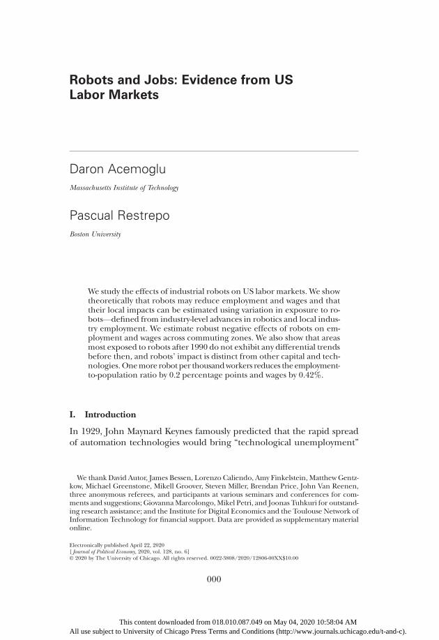
Robotics technology advanced significantly in the 1990s and 2000s, lead-ing to a fourfold rise in the stock of (industrial) robots in the United Statesand western Europe between 1993 and 2007. As figure 1 shows, the increaseamounted to one new robot per thousand workers in the United States and1.6 new robots per thousand workers in western Europe. The automotiveindustry employs 38% of existing robots, followed by the electronics indus-try (15%), plastics and chemicals (10%), and metal products (7%).

Our empirical approach is based on a model where robots and workerscompete in the production of different tasks. Our model builds on Zeira(1998), Acemoglu and Autor (2011), and Acemoglu and Restrepo (2018c)

1 Frey and Osborne (2013), World Development Report (2016), and McKinsey GlobalInstitute (2017) estimate which types of jobs are susceptible to automation on the basisof various technological projections. Such approaches are not informative about the equi-librium impact of automation since they do not take into account how other sectors andoccupations will respond to these changes. See also Arntz, Gregory, and Zierahn (2016) onother problems with these methodologies.

This content downloaded from 018.010.087.049 on May 04, 2020 10:58:04 AM use subject to University of Chicago Press Terms and Conditions (http://www.journals.uchicago.edu/t-and-c).

robots and jobs 000

but extends these frameworks so that the share of tasks performed by robotsvaries across sectors and there is trade between labor markets specializing indifferent industries. Improvements in robotics technology negatively affectwages and employment owing to a displacement effect (as robots directly dis-place workers from tasks that they were previously performing), but there isalso a positive productivity effect (as other industries and/or tasks increasetheir demand for labor). Our framework clarifies that, because of the dis-placement effect, robots can have very different implications for labor de-mand than capital deepening or factor-augmenting technologies. Our modelalso shows that the effects of robotics technologies on employment and wagescan be estimated by regressing the change in these variables on exposureto robots. Exposure to robots is a Bartik-style measure (Bartik 1991), con-structed from the interaction between baseline industry shares in a locallabor market and technological possibilities for the introduction of ro-bots across industries.

We first document that there is considerable variation in robot adop-tion across industries and show that the same industries are rapidly adopt-ing robots in both the United States and Europe. We further show that atthe industry level, there is no strong positive correlation between robotadoption and any of the other major trends affecting US local labor mar-kets, such as import competition from China and Mexico, offshoring,the decline of routine tasks, investments in information technology (IT)capital, and overall capital deepening. Moreover, consistent with theory,robot adoption at the industry level is associated with lower labor shareand employment and greater value added and labor productivity.

After presenting industry-level correlations, we investigate the equilib-rium impact of robots in local labor markets, proxied by commuting zones

FIG. 1.—Industrial robots per thousand workers in the United States and Europe.

This content downloaded from 018.010.087.049 on May 04, 2020 10:58:04 AMAll use subject to University of Chicago Press Terms and Conditions (http://www.journals.uchicago.edu/t-and-c).


All

in the United States.2 We construct our measure of exposure to robots us-ing data from the IFR on the increase in robot usage across 19 industries(roughly at the two-digit level outside manufacturing and at the three-digitlevel within manufacturing) and their baseline employment shares fromthe census before the onset of recent advances in robotics technology.To focus on the component of investment in robots driven by technolog-ical advances, we exploit adoption trends in European economies that areahead of the United States in robotics. Our identifying assumption is thatcommuting zones housing industries with greater advances in roboticstechnology are not differentially affected by other labor market shocksor trends—a presumption that we investigate from a number of angles.3

Using this strategy, we estimate a negative relationship between a com-muting zone’s exposure to robots and its post-1990 labor market out-comes. Our estimates imply that between 1990 and 2007 the increase inthe stock of robots (approximately one additional robot per thousand work-ers from 1993 to 2007) reduced the average employment-to-populationratio in a commuting zone by 0.39 percentage points and average wagesby 0.77% (relative to a commuting zone with no exposure to robots).These estimates are sizable but not implausible. For example, they implythat one more robot in a commuting zone reduces employment by aboutsix workers; this estimate includes both direct and indirect effects, the lat-ter caused by the decline in the demand for nontradables as a result ofreduced employment and wages in the local economy.

To understand the aggregate implications of these estimates, we needto make additional assumptions about how different commuting zones in-teract. Greater use of robots in a commuting zone generates benefits forthe rest of the US economy by reducing the prices of tradable goods pro-duced using robots and by creating shared capital income gains. Our

2 Not all equilibrium responses take place within commuting zones—the most importantother responses are trade with other local labor markets, which we model explicitly below;migration, which we investigate empirically; and the response of technology and new tasksto changes in factor prices emphasized in Acemoglu and Restrepo (2018c). All the same,recent research suggests that much of the adjustment to shocks, in both the short andthe medium run, takes place locally (e.g., Acemoglu, Autor, and Lyle 2004; Moretti 2011;Autor, Dorn, and Hanson 2013).

3 We show in Acemoglu and Restrepo (2018a) that greater robot adoption in thesecountries is largely a consequence of their more rapid demographic change than in theUnited States. Our empirical strategy is similar to that used by Autor, Dorn, and Hanson(2013) and Bloom, Draca, and Van Reenen (2016) to estimate the effects of Chinese im-ports. Though not a panacea for all sources of omitted variable bias, this strategy allows usto filter out variation in robot adoption coming from idiosyncratic US factors (e.g., US-specific declines or worsening labor relations in some industries). This strategy wouldbe compromised if changes in robot usage in other advanced economies were correlatedwith adverse shocks to US industries. For instance, there might be common shocks affect-ing the same industries across advanced economies, such as other technological changesor import competition, and these shocks could induce the same industries everywhereto adopt robots. We show later that these confounders are not responsible for our results.


robots and jobs 000

model enables us to quantify these positive spillovers across commutingzones and leads to smaller but still negative aggregate effects. With ourpreferred specification, our estimates imply that one more robot perthousand workers reduces the aggregate employment-to-population ra-tio by about 0.2 percentage points and wages by about 0.42% (comparedwith its larger local effects, 0.39 percentage points and 0.77%, respec-tively), or equivalently, one new robot reduces employment by about3.3 workers.

We verify that our measure of exposure to robots is unrelated to pasttrends in employment and wages from 1970 to 1990, a period that precededthe onset of rapid advances in robotics technology. Several robustness checksfurther bolster our interpretation. First, our results are robust to includ-ing differential trends by various baseline characteristics, linear com-muting zone trends, and controls for other changes affecting demandor productivity in various industries. Second, we show that the automotiveindustry, which is the most robot-intensive sector, is not driving our results.Third, consistent with our theoretical emphasis that robots (and more gen-erally, automation technologies) have very different labor market effectsthan other types of machinery and overall capital deepening, we find nonegative employment and wage effects from capital, other IT technologies,or overall productivity increases.

The employment effects of robots are most pronounced in manufactur-ing and particularly in industries most exposed to robots. They are alsoconcentrated in routine manual, blue-collar, assembly, and related occupa-tions. Consistent with the presence of spillovers on nontradables, we esti-mate negative effects on construction and retail as well as personal services.

Besides the papers that we have already mentioned, our work is relatedto the empirical literature on the effects of technology on wage inequality(Katz and Murphy 1992), employment polarization (Autor, Levy, andMurnane 2003; Goos and Manning 2007; Autor and Dorn 2013; Michaels,Natraj, and Van Reenen 2014), aggregate employment (Autor, Dorn, andHanson 2015; Gregory, Salomons, and Zierahn 2016), the demand for la-bor across cities (Beaudry, Doms, and Lewis 2006), and firms’ organizationand demand for workers with different skills (Caroli and Van Reenen 2001;Acemoglu et al. 2007; Bartel, Ichniowski, and Shaw 2007).

Most closely related to our work is the pioneering paper by Graetz andMichaels (2018). Focusing on the variation in robot usage across indus-tries in different countries, Graetz and Michaels estimate that industrialrobots increase productivity and wages but reduce the employment oflow-skill workers. Although we rely on the same IFR data, we utilize a dif-ferent empirical strategy, which enables us to go beyond cross-country,cross-industry comparisons and exploit plausibly exogenous changes inthe spread of robots to estimate the equilibrium impact of robots on locallabor markets.



All

The rest of the paper is organized as follows. Section II presents a sim-ple model of the effects of robots on employment and wages. Section IIIintroduces our data and sources. Section IV documents the correlationbetween robot adoption at the industry level and employment, the laborshare, and value added. Section V presents our main empirical resultsand various robustness checks. This section also looks at the differentialeffects of robots on workers in different industries, occupations, and skillgroups. Section VI presents our instrumental variable (IV) estimates andevaluates the local and aggregate implications of the spread of roboticstechnology in the United States. Section VII concludes. The appendix(available online) presents proofs, additional theoretical results, and ro-bustness checks.

II. Robots, Employment, and Wages: A Model

This section presents a model building on Acemoglu and Restrepo (2018c)to exposit the potential effects of robots on employment and wages and de-rives our estimating equations. To develop intuition, we start with a settingwithout trade between commuting zones.

A. Effects of Robots in Autarky Equilibrium

The economy consists of jCj commuting zones. Each commuting zonec ∈ C has preferences defined over an aggregate of the output of jI j in-dustries, given by

Yc 5 oi ∈ I

n1=ji Y j21ð Þ=j

ci

� �j= j21ð Þ, (1)

where j > 0 denotes the elasticity of substitution across goods producedby different industries and the ni’s are share parameters that designatethe importance of industry i in the consumption aggregate (withoi ∈ Ini 5 1).

In the autarky equilibrium, a commuting zone consumes its own pro-duction of each good, denoted by Xci. Hence, for all i ∈ I and c ∈ C, wehave Yci 5 Xci . We choose the consumption aggregate in each commut-ing zone as numeraire (with price normalized to one) and denote theprice of the output of industry i in commuting zone c by PX

ci .Each industry produces output by combining capital with a continuum

of tasks indexed by s ∈ ½0, 1�, each of which can be produced using indus-trial robots or human labor. We use xci(s) to denote the quantity of task sutilized in the production of Xci. These tasks must be combined in fixedproportions so that


robots and jobs 000

Xci 5 a2að1 2 aÞ2ð12aÞAci ½mins ∈ ½0,1�

fxciðsÞg�aK 12aci , (2)

where Kci denotes the nonrobot capital used in industry i, 1 2 a repre-sents its share in the production process, Aci represents the productivityof industry i, and the term a2að1 2 aÞ2ð12aÞ is a convenient normalization.Differences in the Aci’s will translate into different industrial composi-tions of employment across commuting zones.

Industrial robots replace workers in some of the tasks that they werepreviously performing. Specifically, in industry i, tasks [0, vi] are techno-logically automated and can be performed by robots. We assume that allcommuting zones have access to the same technology—that is, the samevi in industry i. Denoting the productivity of labor by gL and the produc-tivity of robots by gM > 0, we have

xciðsÞ 5gMMciðsÞ 1 gLLciðsÞ if s ≤ vi,

gLLciðsÞ if s > vi,

(

where Lci(s) and Mci(s) represent, respectively, the numbers of workersand robots used in task s. Because tasks above vi have not yet been tech-nologically automated, they must be performed by labor.

In each commuting zone c, labor is supplied by a representative house-hold with preferences

C12wc 2 1

1 2 w2

B

1 1 εL11ε

c ,

where Cc denotes this household’s consumption and Lc represents its la-bor supply. Its budget constraint is Cc ≤ WcLc 1 Pc , where Pc is nonlabor(capital and profit) income. In this specification, w determines the in-come elasticity of labor supply, and ε is the inverse of the wage elasticityof labor supply.

Robots are produced using investment (in units of the final good), de-noted by Ic, with the production function Mc 5 Dð1 1 hÞI 1=ð11hÞ

c and havea rental price of RM

c . This formulation, with h > 0, allows the supply of ro-bot services to a commuting zone to be upward sloping. This is reason-able in the medium term, since about two-thirds of the costs of robotsare for services supplied by local, specialized robot integrators that in-stall, program, and maintain this equipment (Leigh and Kraft 2018). Fi-nally, in the autarky model, we take the supply of capital in commutingzone c to be fixed at Kc and denote its price by RK

c .An equilibrium is a tuple of prices fWc , RM

c , R Kc gc ∈ C and quantities

fCc , Yc , Ic , Lc , Mcgc ∈ C, such that in all commuting zones, firms maximizeprofits, households maximize their utility, and the markets for capital, la-bor, robots, and final goods clear:



All

oi ∈ I

ð½0,1�

LciðsÞ 5 Lc , oi ∈ I

ð½0,1�

MciðsÞ 5 Mc , oi ∈ I

KciðsÞ 5 Kc ,

Cc 5 Yc 2 Ic :

We prove in the appendix that an equilibrium exists and is unique.To analyze the equilibrium impact of robots, let us first define cost sav-

ings from using robots in commuting zone c as

pc 5 1 2gLRM

c

gMWc

:

Robots will not be adopted when pc < 0. In what follows, we focus on thecase where pc > 0 in all commuting zones. The next proposition charac-terizes the partial equilibrium impact of an advance in automation/ro-botics technology for industry i, denoted by dvi.Proposition 1. Suppose that pc > 0. Then,

d lnLci 5 2dvi

1 2 vi1

1

ad lnYc 2 j 1

1

a2 1

� �d lnPX

ci , (3)

where Lci denotes the employment in industry i in commuting zone c.Like all other results in this section, a proof of this proposition is pre-

sented in the appendix.Equation (3) highlights three different forces shaping labor demand

of industry i, represented by Lci. First, there is a negative displacementeffect: an increase in vi leads to the use of robots in tasks otherwise per-formed by labor, displacing workers employed in these tasks. This dis-placement effect always reduces the labor share in the industry undergo-ing automation and may also reduce its overall labor demand.4 However,because of the positive productivity effect represented by the second term,labor demand does not necessarily decline following advances in auto-mation technology. Intuitively, automation lowers the cost of production(thus increasing productivity) and via this channel raises the demandfor labor in nonautomated tasks in all industries. Finally, there is a com-position effect, represented by the third term: industries undergoing au-tomation expand at the expense of others, and this raises the demandfor labor coming from their nonautomated tasks.

4 The negative impact on the labor share can be seen by computing total production inindustry i as Xci 5 Acia

2að1 2 aÞ2ð12aÞ fmin½gMMci=vi , gLLci=ð1 2 viÞ�gaK 12aci , which shows

that an increase in vi always makes production less labor intensive (see Acemoglu andRestrepo 2018c, 2019b). In the appendix, we establish that a sufficient condition for the dis-placement effect to dominate the other forces and reduce (relative) industry employment isj < 1 1 ð1 2 pc sLicÞ=apc sLic , where sLic is the industry’s labor share in production tasks. Thiscondition is easily satisfied for plausible parameter values.


robots and jobs 000

We can aggregate the industry-level implications of proposition 1 to de-rive the effects of robots on local labor demand as follows:

d lnLc 52oi ∈ I

‘cidvi

1 2 vi1

1

ad lnYc 2 j 1

1

a2 1

� �oi ∈ I

ð‘ci 2xciÞ d lnPXci , (4)

where ‘ci represents industry i’s share in total employment in commutingzone c, while xci represents this industry’s share of value added in the localeconomy. The first two terms are direct analogues of the displacementand productivity effects in (3). The third term shows that the impact ofthe composition effect for labor demand depends on whether automa-tion is reallocating output toward sectors that are more labor intensivethan average (those for which ‘ci > xci). This composition effect disap-pears when all industries have the same labor share.

Equation (4) provides a partial equilibrium characterization of howthe demand for labor changes following automation. The next proposi-tion links changes in prices and total output to automation technologiesand thus derives the full equilibrium impact of automation.Proposition 2. Suppose that pc > 0 for all c ∈ C and that vi 5 0 for

all i ∈ I . Then,

d lnLc 5 ½2zdisp 1 z prodpc 2 z incc,Lw� � o

i ∈ I‘ci

dvi1 2 vi

gL

gM

, (5)

d lnWc 5 ½2zdispε 1 z prodεpc 1 z incc,Ww� � o

i ∈ I‘ci

dvi1 2 vi

gL

gM

, (6)

where zdisp 5 ð1 2 a 1 hÞ=L, z prod 5 ð1 1 hÞ=L, z incc,L 5 apc=Lc , z inc

c,W 5aðpc 2 ð1 2 pcÞð1 2 a 1 hÞÞ=L, and L 5 ðgL=gM Þð1 2 a 1 aw 1 εÞ > 0.

The assumption that vi 5 0 for all i simplifies the relevant expressionsby removing the composition effect. The economic effects are similarwhen this assumption is relaxed, as shown in the appendix.5

Proposition 2 establishes that the response of both employment andwages to automation is shaped by the term oi ∈ I‘ci½dvi=ð1 2 viÞ�ðgL=gM Þ,which is the basis of our measure of exposure to robots. In addition, thecoefficient on this variable in both equations comprises three distinctterms. The first term, 2zdisp, represents the displacement effect. The sec-ond, zprod, represents the productivity effect, generated by cost savings,pc. When cost savings from automation are limited, automation decreasesemployment and wages. Conversely, whenpc is large, automation increases

5 Composition effects arise when the term ‘ci 2 xci (or equivalently, the labor share) iscorrelated with the introduction of robots across industries. The correlation betweenthe labor share of an industry in 1992 and subsequent robot usage is 0.1 across all indus-tries and 20.04 within manufacturing, suggesting a minor role for composition effects.



All

them. Finally, the third term in both equations incorporates the negativeincome effect of automation on labor supply.

The impacts of robots highlighted in proposition 2 are very differentfrom the effects of overall capital deepening (an increase in the supplyof capital, Kc) or from technological changes that increase the productiv-ity of robots (gM) or industry productivity (Aci). Capital deepening, greaterproductivity of robots, and increases in industry productivity do not dis-place workers from the tasks they are performing and always raise wagesand employment.6 This observation clarifies that the displacement effectcreated by automation is responsible for its potentially negative impact onlabor demand.

B. Effects of Robots When Commuting Zones Trade

The autarky model transparently illustrates the displacement and produc-tivity effects of automation but ignores how its economic consequencesmay spill over across local labor markets. Trade in goods and serviceschanges the sensitivity of employment and wages to robot adoption andtheir aggregate implications. We now incorporate automation/robots intoa simple model of trade between commuting zones building on Arming-ton (1969) and Anderson (1979). Specifically, we modify our model in twoways. First, we assume that the representative household’s utility dependson a tradable good, Cc, and a nontradable (service) good, Sc:

ðCfc S12f

c Þ12w 2 1

1 2 w2

B

1 1 εL11ε

c : (7)

This specification implies that a constant share f ∈ ð0, 1Þ of spendinggoes to the tradable good. We assume that this nontradable good is pro-duced with labor—that is, Sc 5 LS

c —and we denote the price of the non-tradable good in commuting zone c by Pc. The remaining labor, Lc 2 LS

c ,is used in the production of tradable goods.

The second modification is to assume that the tradable good is producedas in (1) but now with inputs sourced from all commuting zones so that

Yci 5 os ∈ C

u1=lsi Xsci

l21ð Þ=l� �l= l21ð Þ

ðfor all c and iÞ, (8)

where l is the elasticity of substitution between varieties sourced from dif-ferent commuting zones and the share parameters—the usi’s—indicate

6 As we show in Acemoglu and Restrepo (2018b, 2019b), labor-augmenting technolog-ical changes have very different effects from automation as well unless the elasticity of sub-stitution between labor and machines is implausibly low (in particular, lower than the shareof machines in value added). Here we took this elasticity to be zero for simplicity, since thissimplification does not impact any of the implications we are focusing on.


robots and jobs 000

the desirability of varieties from different sources. We assume that thereare no trade costs, so that the price of the tradable good is equalizedacross commuting zones, and we choose it as the numeraire. Denotingthe amount of good i exported from commuting zone c to destinationd by Xcdi (including d 5 c), market clearing imposes

Xci 5 od ∈ C

Xcdi ðfor all c and iÞ:

We also assume that the initial stock of capital of the economy, K, isperfectly mobile across commuting zones, and we modify the budgetconstraint of households to Cc 1 PcSc ≤ WcLc 1 xP

c P, where P is the na-tional nonlabor income and a share xP

c of this income is allocated tocommuting zone c (with oc ∈ CxP

c 5 1). The main result of this section ispresented in the next proposition, which parallels proposition 2.Proposition 3. Suppose that pc 5 p0 for all c ∈ C and that vi 5 0 for

all i ∈ I . Then,

d lnLc 5 ½2�zdispf 1 �zprodfp0 2 �z incL w�o

i ∈ I‘ci

dvi1 2 vi

gL

gM

1 �zYL d lnY

1 �zPLd lnP 1 �z

pricecL ,

(9)

d lnWc 5 ½2�zdispε 1 �z prodεp0 1 �z incW w�o

i ∈ I‘ci

dvi1 2 vi

gL

gM

1 �zYW d lnY

1 �zPW d lnP 1 �z

pricecW ,

(10)

where the �z’s are functions of the underlying parameters.This proposition assumes that pc is the same across commuting zones

as well as vi 5 0 for all i; we provide a more general version with similarimplications in the appendix.

As before, the �z’s summarize the local impact of robots on employmentand wages. Trade between commuting zones implies that productivitygains and price changes in one area will be shared with others. The pro-ductivity spillovers, generated by the change in national income d ln Y,are captured by the �zY terms, while spillovers from changes in pricesare summarized by the �z price terms. Finally, the �zP terms represent the in-come effects and the demand for nontradables resulting from nonlaborincome, d ln P. These general equilibrium effects are not functions of ex-posure to robots in the own commuting zone, and thus we obtain thesame reduced-form relationship between robots and local labor demandas in the autarky model. The aggregate effects of robots, however, dependon the extent of trade across commuting zones because of the additionalspillover terms and because the �z’s in this proposition differ from theirautarky counterparts in proposition 2. We take these differences into ac-count in our quantitative evaluation.

(10)

(9)



All

C. Empirical Specification

Propositions 2 and 3 summarize the effects of advances in the roboticstechnology on local employment and wages. The key equations, (9) and(10), show that the equilibrium impact of robots depends on the sameobject, which we will call a commuting zone’s US exposure to robots,

US exposure to robotsc 5 oi ∈ I

‘ci � APRi (11)

(recall that ‘ci is the baseline employment share of industry i in commut-ing zone c), and

APRi 5dvi

1 2 vi

gL

gM

5dM i

Li

2dYi

Yi

Mi

Li

(12)

is the (US) adjusted penetration of robots in industry i. Exposure to ro-bots is thus a Bartik-style measure combining industry-level variation inthe usage of robots and baseline employment shares. Our model impliesa specific form for this relationship, including an adjustment for the over-all expansion of each industry’s output, given by the last term in (12).

With this measure of exposure to robots, we can estimate

d lnLc 5 bL � US exposure to robotsc 1 eLc ,

d lnWc 5 bW � US exposure to robotsc 1 eWc ,

(13)

regardless of whether there is trade between commuting zones, thoughthe coefficients bL and bW have different interpretations in these two cases.In these equations, eLc and eWc represent other factors affecting labor sup-ply and demand, and in our empirical work, we model them as functionsof various baseline characteristics and observed economic changes.

The models in equation (13) can be estimated using ordinary leastsquares (OLS) with the variable for US exposure to robots computedfrom US data on the adjusted penetration of robots. Yet there are two re-lated reasons why the US exposure to robots could be correlated with theerror terms, eLc and eWc , leading to biased estimates. First, some industriesmay be adopting robots in response to other changes that they are under-going, which could directly impact their labor demand. Second, any shockto labor demand in a commuting zone affects the decisions of local busi-nesses, including robot adoption.7

(13)

7 An example of the first concern would be the automotive industry adopting more ro-bots in the United States because of greater wage push from its unions. An example of thesecond would be a local recession in Detroit, Michigan, that impacts the automotive indus-try that has a large footprint there.


robots and jobs 000

Ideally, we want to use changes in robot penetration only driven by ex-ogenous improvements in technology, dvi. To identify the component ofrobot penetration driven by changes in technology, we instrument the USexposure to robots using an analogous measure constructed from thepenetration of robots in European countries that are ahead of the UnitedStates in robotics technology. To do so, we construct

Exposure to robotsc 5 oi ∈ I

‘ci � APRi, (14)

where APRi represents the adjusted penetration of robots computedfrom European countries. We describe and motivate this choice in greaterdetail in the next section.

III. Data

In this section, we describe our main data sources.

A. Robots

Our main data consist of counts of the stock of robots by industry, country,and year from the IFR. The IFR data are based on yearly surveys of robotsuppliers and cover 50 countries from 1993 to 2014, corresponding toabout 90% of the industrial robots market. However, the stock of industrialrobots by industry going back to the 1990s is available only for Denmark,Finland, France, Germany, Italy, Norway, Spain, Sweden, and the UnitedKingdom, which together account for 41% of the world industrial robotmarket.8 Outside of manufacturing, we have data for the use of robots insix broad industries: agriculture, forestry, and fishing; mining; utilities; con-struction;education,research,anddevelopment;andservices.Withinman-ufacturing, we have data on the use of robots for 13 more disaggregatedindustries: food and beverages, textiles (including apparel), wood and fur-niture, paper and printing, plastics and chemicals, minerals, basic metals,metal products, industrial machinery, electronics, automotive, shipbuild-ing and aerospace, and miscellaneous manufacturing (e.g., production ofjewelry and toys). We use this industry classification throughout and referto it as the “IFR industries.”

Figure 1 and table A1 (tables A1–A34 are available online) depict theevolution of robot stocks for different groups of European countriesand for the United States. In figure 1, we separately show the evolutionof the stock of robots for Germany; for the United States; the average

8 Though the IFR also reports data by industry for Japan, these data underwent a majorreclassification. We follow the recommendations of the IFR and exclude Japan from ouranalysis.



All

for Denmark, Finland, France, Italy, and Sweden; and the average forNorway, Spain, and the United Kingdom. The trends for Denmark, Fin-land, France, Germany, Italy, and Sweden are particularly interesting, be-cause these countries are technologically more advanced than the UnitedStates in robotics.9 US robot usage starts near 0.4 robots per thousandworkers in the early 1990s, increases to 0.7 in 2000, and then rises rapidlyto 1.4 in the late 2000s; this evolution closely tracks the average of Den-mark, Finland, France, Italy, and Sweden, but its level is about 20% lower.10

The IFR data have some noteworthy shortcomings. First, not all robotsare classified into one of the 19 IFR industries. About 30% of robots areunclassified, and this percentage has declined throughout our sample.We allocate these unclassified robots to industries in the same propor-tions as in the classified data. Second, although the IFR reports data onthe total stock of industrial robots in the United States from 1993 onward,it does not provide industry breakdowns until 2004. This does not affectthe measure of exposure to robots computed from European data, and insection VI.A we describe how we use US data in our IV strategy. Finally, theIFR reports only the overall stock of robots for North America. Thoughthis aggregation introduces noise in our measures of US exposure to ro-bots, this is not a major concern, since the United States accounts formore than 90% of the North American market and our IV procedurepurges this type of measurement error from the US exposure to robots.11

We combine the IFR data with employment counts and output by coun-try and industry from the European Union–level analysis of capital, labor,energy, materials, and service inputs (EU KLEMS) Growth and Productivity

9 These countries have more robots than the United States at the beginning of the sam-ple in 1993 and have invested more in robots since. They also have greater “robot exports”(measured as exports of intermediates related to robotics from the Comtrade data set; fordetails, see Acemoglu and Restrepo 2018a). For example, robot exports per worker arethree to four times as large in Italy, France, and Denmark as in the United States and morethan six times as large in Germany, Finland, and Sweden. Norway and the United Kingdomare behind the United States in all of these metrics. Spain has adopted robots rapidly in theautomotive industry since 1993 but is behind or comparable to the United States in othersectors, and its robot exports are at the same level as the United States.

10 Acemoglu and Restrepo (2018a) show that demographic factors account for a largefraction of this cross-country variation and for why European countries are ahead of theUnited States in robotics. The relative shortage of middle-aged (production) workers incountries that are aging rapidly—e.g., Germany, France, Italy, Japan, and South Korea—en-courages the development and adoption of robotics technology, which is then exported toother countries, including the United States, experiencing less rapid demographic change.

11 Robots in different sectors have similar capabilities and prices. Industrial robots be-long to one of a handful of standardized types—articulated robots, selective compliance as-sembly robot arm (SCARA) robots, Cartesian robots, and parallel robots. Consistent withthis, robot prices are fairly similar across sectors (ranging from about $44,000 per robotto about $88,000), and our results in table 5 suggest that the quantitative effects of robotsin different sectors are similar. We investigate the role of robot prices further in tables A24and A25.


robots and jobs 000

Accounts (see Jägger 2016),12 which allows us to measure the adjusted pen-etration of robots, APRi and APRi, for different time periods. Followingequation (12), our baseline measure of the adjusted penetration of robotsbetween two dates, t0 and t1, is given by

APRi,ðt0,t1Þ 51

5 oj∈EURO5

Mji,t1 2 M

ji,t0

Lji,1990

2 gj

i,ðt0,t1ÞMi,t0

Lji,1990

� �, (15)

where Mji,t represents the number of robots in industry i in country j at

time t (from the IFR data), g j

i,ðt0,t1Þ is the growth rate of output of industry iin country j between t0 and t1 (from the EU KLEMS), and L

ji,1990 represents

the baseline employment level in industry i and country j (also from theEU KLEMS).13 In our long-differences models, we take t0 5 1993 and t1 52007, though we also present models where we focus on other periods.

For our baseline measure, we use the average penetration in EURO5,comprising Denmark, Finland, France, Italy, and Sweden—that is, coun-tries ahead of the United States in robotics, excluding Germany. Focus-ing on countries that are ahead of the United States helps us isolatethe source of variation coming from global technological advances (ratherthan idiosyncratic US factors). We exclude Germany from our baselinemeasure because, as figure 1 shows, it is so far ahead of the other countriesthat its adoption trends may be less relevant for US patterns than thetrends in EURO5. The appendix presents versions of our main resultsfor different constructions of the APRi measure, including a specificationwhere we use all European countries, one where we use both Germanyand the EURO5, one where we use the observed increase in robot densitywithout the g j

i,ðt0,t1ÞMi,t0=Lji,1990 term, and a complementary measure where

12 To obtain comparable data, we use information on hours worked to obtain a count ofUS-equivalent workers by industry in 1990. We then compute the number of robots by in-dustry, country, and year divided by US-equivalent workers in 1990. Because the data forNorway are missing from the EU KLEMS, we use the distribution of employment in theremaining Scandinavian countries in our sample (Denmark, Finland, and Sweden) to im-pute the Norwegian distribution. In addition, we were able to match most of the industriesused in the EU KLEMS data set to the 19 IFR industries. One exception is wood and fur-niture, since employment in furniture products is pooled with miscellaneous manufactur-ing. To address this issue, we allocate 40% of the employment in miscellaneous manufac-turing to the wood and furniture sector based on the proportions of employment in theUnited States in these detailed industries (obtained from the National Bureau of Eco-nomic Research–Center for Economic Studies [NBER-CES] data set described below). Fi-nally, because the IFR data for Denmark are not classified by industry before 1996, we con-struct estimates for 1993–95 by deflating the 1996 stocks by industry using the total growthin its stock of robots.

13 Because there were few robots in 1993, the adjustment term g j

i,ðt0 ,t1ÞMi,t0=Lji,1990 is not

quantitatively important; 96% of the variation in the adjusted penetration of robots acrossindustries between 1993 and 2007 is driven by the increase in robot density—the termðMj

i,t1 2 Mji,t0Þ=Lj

i,1990 in eq. (15). The exception is the electronics industry, which had a highstock of robots in 1993 and experienced rapid growth thereafter.



All

we include an adjustment for variation in the average price of a robot acrossindustries.

We also measure the US adjusted penetration of robots as

APRUSi,ðt0,t1Þ 5

MUSi,t1 2 MUS

i,t0

LUSi,1990

2 g USi,ðt0,t1Þ

Mi,t0

LUSi,1990

: (16)

Given the coverage of the IFR data for US industries, this variable goesback only to t0 5 2004.

B. Industry Data

To explore the industry-level correlates of robot adoption, we use data onUS industry employment, wage bill, value added, and labor share. Theemployment and wage bill data come from the County Business Patterns(CBP). We supplement the CBP with the NBER-CES data set, which coversthe manufacturing sector and reports data on employment and wage billsfor all workers and for production workers (see Acemoglu et al. 2016). Wealso use data on value added and labor shares from the Bureau of EconomicAnalysis input-output (BEA-IO) tables and on IT capital and the overallcapital stock from the Bureau of Labor Statistics. These data are availablefor a detailed set of industries, which we then aggregate to the 19 IFR in-dustries. Industry-level imports from China and Mexico and exports fromGermany, Japan, and South Korea are computed from Comtrade data(following Acemoglu et al. 2016). Finally, we use the share of tasks in anindustry that can be offshored (“task offshorability” from Autor and Dorn2013) and the share of imported intermediates as a proxy for offshoring(from Feenstra and Hanson 1999; Wright 2014).

C. Commuting Zone Data and Exposure to Robots

In our main analysis, we focus on the 722 commuting zones covering theUS continental territory (Tolbert and Sizer 1996). Following equations (11)and (14), we measure US exposure to robots in a commuting zone as

US exposure to robotsc,ðt0,t1Þ 5 oi ∈ I

‘1990ci � APRi,ðt0,t1Þ, (17)

where ‘1990ci represents industry i’s share in the total employment of com-

muting zone c and APRi is as defined in (16). Exposure to robots is de-fined analogously, exploiting variation in industry-level adoption of ro-bots in the EURO5 countries,

Exposure to robotsc,ðt0,t1Þ 5 oi ∈ I

‘1970ci � APRi,ðt0,t1Þ, (18)

whereAPRi,ðt0,t1Þ is given in (15). We now use the 1970 employment shares,‘1970ci , as the baseline to focus on historical, persistent differences in the


robots and jobs 000

industrial specialization of commuting zones that predate robotics tech-nology. This choice avoids any mechanical correlation due to robot adop-tion before the 1990s or mean reversion associated with temporary changesin industry employment in the 1980s. It is also worth noting that even whenwe consider changes in subperiods (e.g., in our models with stacked differ-ences), we keep the baseline employment shares constant to avoid endog-enous and serially correlated changes in our exposure variable.

We use the public use data from the 1970, 1990, and 2000 censuses andthe American Community Survey (ACS; see Ruggles et al. 2010) to con-struct measures of population, employment, employment by industry andoccupation, and demographics for each commuting zone. To increasesample size, we follow Autor, Dorn, and Hanson (2013) and measure the2007 outcomes using the ACS for 2006–8. Similarly, we measure the 2014outcomes from the ACS for 2012–16. We also use the census and ACS tocompute the average hourly and weekly wages within 250 demographic �commuting zone cells, which corrects for changes in the observed charac-teristics of employed workers. Our demographic cells are defined by gen-der, education (less than high school, high school degree, some college,college or professional degree, and masters or doctoral degree), 10-yearage bins (16–25, 25–35, 36–45, 46–55, 56–65, and >65), and race. All top-coded wage income observations are set equal to 1.5 times the value of thetop code, and we also winsorized wages at $2 per hour as in Acemoglu andAutor (2011). We additionally use county-level data (which we again aggre-gate to the commuting zone level) on employment counts from the CBPfor 1990, 2000, and 2007; wage and nonwage income from the BEA; andwage income and migration flows from the Internal Revenue Service (IRS).

To control for potentially confounding changes in trade patterns andother technological changes, we rely on data on exposure to Chinese im-ports from Autor, Dorn, and Hanson (2013) and data on the fraction ofemployment in a commuting zone in routine occupations (as defined inAutor and Dorn 2013). To distinguish the effects of robots from the ef-fects of capital accumulation, investments in IT, and other technologiesraising productivity, we construct Bartik measures of increases in capitalstocks, IT capital, and value added across the 19 IFR industries.

Finally, we use data compiled by Leigh and Kraft (2018), who scrapedthe web to obtain the location and employment of robot integrators—companies that install, program, and maintain robots. Using these data,we construct estimates of robot integrator activity in each commutingzone.

IV. Industry Correlations

We start by documenting industry trends. Figure 2 depicts the relation-ship between APRi,ð1993,2007Þ (computed from EURO5) and APRi,(2004,2007)



All

(computed from the US data and scaled to a 14-year equivalent change).Both variables are expressed in terms of robots per thousand workers.Consistent with the notion that US industry trends in robotics are drivenby technological improvements, there is a positive correlation betweenadoption of robots in the EURO5 countries and in the United States(see also table A2). The figure also reveals significant heterogeneity acrossindustries. While some industries—such as automotive, plastics and chem-icals, and metal products—exhibit increases in robot penetration of morethan 7.5 robots per thousand workers, others—such as paper and print-ing, textiles and wood, and furniture—experienced modest increases inboth Europe and the United States.

FIG. 2.—Adjusted penetration of robots in the United States and EURO5 by industry.Plot of the adjusted penetration of robots between 1993 and 2007 (APRi) and the adjustedpenetration of robots in the United States between 2004 and 2007 (APRi rescaled to a 14-yearequivalent change). Adjusted penetration of robots is given in number of robots per thou-sand workers in the industry. The solid line corresponds to the 457 line. Circle size indicatesthe baseline US employment in the industry.


robots and jobs 000

In the rest of this section, we focus on the variation in APRi , which weinterpret as a proxy for improvements in robotics technology availableto US firms. Table A3 documents that improvements in robotics do notmimic other industry-level trends. Industries that are adopting more robotsare not those affected by Chinese or Mexican import competition or off-shoring, nor those experiencing rapid growth in total capital or IT capital,nor those with a large fraction of routine jobs. Within manufacturing, thecorrelation between our measure of adjusted penetration of robots, APRi,and the change in imports from China is 20.39 (the overall correlationis 0.15). The correlation of APRi with the share of routine tasks is 20.24within manufacturing and20.01 overall. The correlations with the changein imports from Mexico, with task offshorability, and with offshoring ofintermediates are, respectively, 20.03, 20.41, and 20.17 within manufac-turing (and 0.31, 20.26, and 0.19 overall). The correlation with the in-crease in capital is 0.22 within manufacturing (and 20.37 overall), andthe correlation with the increase in ITcapital is 0.23 within manufacturing(and 20.17 overall). These patterns strengthen our presumption that theuse of industrial robots is a technological phenomenon that is largely un-related to other industry trends.14

Our model shows that under plausible conditions, industries that adoptrobots reduce their labor demand. Table 1 reports regressions of variousindustry-level measures of labor demand on APRi for different time peri-ods. Panel A focuses on the wage bill, and panel B looks at employment.Columns 1–4 present long-differences specifications where we regress thechange in log wage bill from 1993 to 2007 on our baseline measure of ad-justed robot penetration for the same period,APRi,ð1993,2007Þ. In column 1 ofpanel A, we show the relationship betweenAPRi and log wage bill, which isnegative, indicating that industries experiencing greater penetration ofrobots have also seen significant (relative) declines in labor demand. Tocontrol for other industry trends over this time period, column 2 includesthe change in imports from China and dummies for manufacturing andlight manufacturing—the latter consists of the textile industry and thepaper, publishing, and printing industry. These two light manufacturingindustries have been on a steep downward trend for reasons unrelated torobots (mostly because of offshoring and trade from China and the riseof digital media). Controlling for the light manufacturing dummy ensuresthat the estimates in column 2 are not driven by the comparison of thesedeclining industries to other manufacturing industries. Including thesethree controls reduces the magnitude of the coefficient on APRi but also

14 This interpretation is also in line with the close association between APRi and Graetzand Michaels’s (2018) replaceability index, which measures the fraction of occupations inan industry involving tasks that can be automated using industrial robots. See fig. A1 (figs. A1–A4 are available online).


000

This content downloaded from 018.010.087.049 on May 04, 2020 10:58:04 AMAll use subject to University of Chicago Press Terms and Conditions (http://www.journals.uchicago

(.65

4)(.

347)

(.33

9)(.

261)

(.60

9)(.

129)

(.32

9)(.

114)

(.15

2)(.

281)

TA

BL

E1

Robots,LaborDemand,LaborShare,andValueAdded:Industry-LevelResults

Lo

ng

Dif

fere

nce

s,19

93–20

07St

acke

dD

iffe

ren

ces,

1993

–20

00an

d20

00–20

07

Lo

ng

Dif

fere

nce

s,19

92–20

07

CB

P(A

llIn

du

stri

es)

NB

ER

-CE

S(w

ith

inM

anu

fact

uri

ng)

CB

P(A

llIn

du

stri

es)

NB

ER

-CE

S(w

ith

inM

anu

fact

uri

ng)

BE

A-I

O

All

Wo

rker

s(1

)

All

Wo

rker

s(2

)

All

Wo

rker

s(3

)

Pro

du

ctio

nW

ork

ers

(4)

All

Wo

rker

s(5

)

All

Wo

rker

s(6

)

All

Wo

rker

s(7

)

All

Wo

rker

s(8

)

Pro

du

ctio

nW

ork

ers

(9)

All

Wo

rker

s(1

0)

A.

Ch

ange

inL

og

Wag

eB

ill

Val

ue

Ad

ded

Ad

just

edp

enet

rati

on

of

rob

ots

,APR

i2

2.71

82

.923

2.8

162

.993

22.

510

21.

096

21.

492

21.

037

21.

150

.128

(.73

2)(.

419)

(.37

8)(.

324)

(.67

3)(.

235)

(.48

1)(.

177)

(.20

5)(.

061)

Ob

serv

atio

ns

1919

1313

3838

3826

2619

R2

.19

.91

.84

.91

.53

.90

.95

.87

.91

.72

B.

Ch

ange

inL

og

Em

plo

ymen

tL

abo

rSh

are

Ad

just

edp

enet

rati

on

of

rob

ots

,APR

i2

1.96

72

.754

2.8

312

.991

21.

904

2.8

832

1.32

52

.921

21.

016

2.7

97

.edu/t-and-c).

000

This content downloaded from 018.010.087.049 on May 04, 2020 10:58:04 AMAll use subject to University of Chicago Press Terms and Conditions (http://www.journals.uchic

Ob

serv

atio

ns

1919

1313

3838

3826

2619

R2

.12

.90

.87

.92

.30

.86

.93

.89

.93

.37

Co

vari

ates

Tim

ep

erio

dd

um

mie

s✓

✓✓

✓✓

Bro

adin

du

stry

du

mm

ies

✓✓

✓✓

✓✓

✓✓

Ch

ines

eim

po

rts

✓✓

✓✓

✓✓

✓✓

Ind

ust

ryfi

xed

effe

cts

✓

Note.—

Th

ista

ble

pre

sen

tses

tim

ates

of

the

rela

tio

nsh

ipb

etw

een

adju

sted

pen

etra

tio

no

fro

bo

tsan

dth

ew

age

bil

l,em

plo

ymen

t,va

lue

add

ed,a

nd

lab

or

shar

eac

ross

US

ind

ust

ries

.Co

lum

ns

1–4

pre

sen

tlo

ng-

dif

fere

nce

ses

tim

ates

for

chan

ges

inth

elo

gw

age

bil

lfo

r19

93–20

07(p

anel

A)

and

log

emp

loym

ent

for

1993

–20

07(p

anel

B).

Co

lum

ns

5–9

pre

sen

tst

acke

d-d

iffe

ren

ces

esti

mat

esfo

rch

ange

sin

the

log

wag

eb

illf

or

1993

–20

00an

d20

00–20

07(p

anel

A)

and

log

emp

loym

ent

for

1993

–20

00an

d20

00–20

07(p

anel

B).

Co

lum

n10

pre

sen

tslo

ng-

dif

fere

nce

ses

tim

ates

for

chan

ges

inlo

gva

lue

add

edfo

r19

92–20

07(p

anel

A)

and

lab

or

shar

efo

r19

92–20

07(p

anel

B).

Ch

ange

sin

log

valu

ead

ded

are

ann

ual

ized

and

give

nin

per

cen

tch

ange

per

year

.Ch

ange

sin

lab

or

shar

ear

ein

per

cen

tage

po

ints

.D

ata

sou

rces

and

tim

ep

erio

ds

are

rep

ort

edat

the

top

of

the

tab

le,

and

the

set

of

cova

riat

esis

rep

ort

edat

the

bo

tto

m.

Co

lum

n1

do

esn

ot

incl

ud

ean

yco

vari

ates

,an

dco

l.5

incl

ud

eso

nly

tim

ep

erio

dd

um

mie

s.C

olu

mn

s2–

4,6–

9,an

d10

con

tro

lfo

rd

um

mie

sfo

rm

anu

fac-

turi

ng

and

ligh

tm

anu

fact

uri

ng

(pap

er/

pri

nti

ng

and

text

iles

)an

dex

po

sure

toC

hin

ese

imp

ort

sb

yin

du

stry

fro

mA

cem

ogl

uet

al.

(201

6).

Co

lum

n7

in-

clu

des

afu

llse

to

fin

du

stry

fixe

def

fect

s.T

he

regr

essi

on

sin

cols

.1–9

are

wei

ghte

db

yb

asel

ine

ind

ust

ryem

plo

ymen

tin

1993

,an

dth

ere

gres

sio

ns

inco

l.10

are

wei

ghte

db

yb

asel

ine

valu

ead

ded

by

ind

ust

ryin

1992

.Sta

nd

ard

erro

rsth

atar

ero

bu

stag

ain

sth

eter

osk

edas

tici

tyan

dse

rial

corr

elat

ion

atth

ein

du

stry

leve

lar

egi

ven

inp

aren

thes

es.

ago.edu/t-and-c).


All

makes it more precisely estimated (20.923, standard errors 5 0:419). Thisestimate implies that an increase of one robot per thousand workers inour APRi measure is associated with a 0.92% relative decline in the wagebill. Therefore, the average increase in the stock of robots in manufac-turing—seven robots per thousand workers—is associated with a 6.3% de-cline in the wage bill. Columns 3 and 4 show similar patterns for the wagebill of all workers and production workers within manufacturing usingthe NBER-CES data set.

Columns 5–9 present stacked-differences models for two subperiods of7 years, 1993–2000 and 2000–2007, with analogues of ourAPRi variable com-puted for each subperiod (in this case, we have two observations per indus-try). These models are appealing because they focus on within-industrychanges and exploit the timing of robot adoption. For instance, robot pen-etration in the automotive industry accelerated in the 2000s, whereas it de-celerated in shipbuilding and aerospace during the 2000s. We now see amore precisely estimated relationship than the one shown in columns 1–4. For example, the equivalent of the estimate in column 2 is 21.096(standard errors 5 0:235), which implies that one more robot per thou-sand workers (in APRi) is associated with a 1.1% decline in labor demand.Stacked-differences models also enable us to include industry trends, thusmore flexibly controlling for the possibility that industries have been ondifferential trends for other reasons (and in particular controlling for de-clining industries). Although specifications controlling for industry trendsare demanding, in column 7 we estimate a similar negative relationship be-tween robot adoption and labor demand. Finally, columns 8 and 9 showsimilar patterns for the wage bill of all workers and production workerswithin manufacturing using the NBER-CES data set. Panel B shows analo-gous results for employment, and figure 3 visually illustrates the relation-ship between APRi and log wage bill and log employment from column 8.

In the appendix, we present a series of robustness checks for these indus-try correlations. Figure A2 verifies that there are no significant pretrendscorrelated with the adjusted penetration of robots for log wage bill andlog employment (for all workers and for production workers). Tables A4and A5 confirm that the patterns shown in table 1 are similar when weuse different constructions for the APRi variable and when we focus onmore recent time periods. Finally, table A6 shows that the results are alsosimilar when, rather than including the light manufacturing dummy, wedirectly control for industry value added or the factors affecting value addedtrends. In particular, in panel A we control for the change in industry valueadded between 1992 and 2007 (from the BEA-IO tables), and in panel Bwe instrument for the change in value added using intermediate importsin supplier industries. The estimates are broadly similar to but larger thanthe estimates in table 1, presumably because controlling for value addedisolates the displacement effect. In panel C, we control for differences in


FIG. 3.—Relationship between robots and labor demand across industries. This figurepresents residual plots of the relationship between adjusted penetration of robots (APRi)and the change in log wage bill (A) and the change in log employment (B) from stacked-differences models, with data for 1993–2000 (in light gray) and 2000–2007 (in dark gray).The solid line shows the coefficient estimates from column 8 of panel A (A) and column 8of panel B (B) of table 1. The covariates from these models are partialed out. The dashed lineis for a regression that additionally excludes the automotive industry. Circle size indicates thebaseline US employment in the industry.



All

task offshorability, which is one of the factors leading to the rapid declinein production and value added in the light manufacturing industries,while in panel D we include a dummy for industries adopting robots.The results are again similar.

We also use the BEA data to estimate the relationship between robotsand industry labor share and value added between 1992 and 2007. Col-umn 10 in panel A of table 1 shows that, consistent with robots raisingproductivity, value added is increasing in industries adopting more ro-bots—even though employment is contracting.15 This result suggeststhat, as in our theory, industries adopting robots are becoming not onlymore productive but also less labor intensive. This is confirmed by our es-timate in column 10 in panel B, which shows a large decline in the laborshare. This estimate implies that one more robot per thousand workers isassociated with a 0.8 percentage point decline in the labor share between1992 and 2007.

Although we view the industry correlations mostly as descriptive, theyestablish that industries where robotics technology has made greater ad-vances have experienced expanding output and declining labor demand,employment, and labor share. We next turn to the implications of robotsfor employment and wages in local labor markets.

V. Effect of Robots across Commuting Zones

In this section, we describe our measure of exposure to robots and docu-ment its variation. We then present reduced-form results for employmentand wages, investigate their robustness, and explore the heterogeneouseffects of robots across industries, occupations, gender, and skill groups.We present IV estimates and discuss their quantitative implications in thenext section.

A. Exposure to Robots and Robot-Related Activities

We focus on the exposure measure defined in equation (18) and con-structed from European data on robot penetration by industry. We usethis variable as an instrument to uncover the effects of the spread of ro-bots on US labor markets.

15 Within manufacturing, the industries that adopted the greatest number of robots (in theUnited States and in EURO5)—automotive, plastics and chemicals, and metal products—ex-perienced the fastest growth in value added between 1992 and 2007, ranging between 2% and4% per year. In contrast, light manufacturing industries—textiles and paper and printing—did not adopt many robots and experienced absolute declines in value added. In table A7,we also document the significant positive effect of robots on labor productivity, which con-firms one of the main findings of Graetz and Michaels (2018) from cross-industry, cross-countrydata. Because of data availability, we focus on long differences for value added, labor productiv-ity, and labor share.


robots and jobs 000

Figure 4 depicts the geographic distribution of exposure to robots be-tween 1993 and 2007. In many parts of the United States, there is only asmall increase of about 0.27–0.67 robots per thousand workers. In others,including parts of Kentucky, Louisiana, Missouri, Tennessee, Texas, Vir-ginia, and West Virginia, our measure of exposure ranges between twoand five robots per thousand workers. More strikingly, in some parts ofthe rust belt and Texas, robot penetration increases by five to 10 per thou-sand workers. Figure 2 highlighted that there is greater penetration of

FIG. 4.—Geographic distribution of exposure to robots, 1993–2007. A, Distribution of ex-posure to robots. B, Distribution of exposure to robots outside of the automotive industry.



All

robots in the automotive industry than in other sectors (in both the UnitedStates and Europe). Figure 4B verifies that even after this industry is leftout, there is still considerable geographic variation in exposure to robots.

Are commuting zones with a high exposure to robots adopting moreindustrial robots, as our model predicts? Though data on robot adoptionat the commuting zone level are not available, in figure 5 we provide ev-idence of greater robot-related activities in exposed commuting zonesusing the data on integrators from Leigh and Kraft (2018). The figureshows the residual plot of a regression of log of one plus the number ofintegrators in a commuting zone against exposure to robots (as in mostfigures that follow, we partial out the covariates from our main specifica-tion in col. 4 of table 2, which we describe below). The dashed line corre-sponds to the regression relationship after the top 1% of commutingzones with highest exposure to robots are excluded.16 In both cases, wesee a positive association between exposure to robots and the numberof integrators in a commuting zone. Table A8 shows that this relationship

FIG. 5.—Exposure to robots and the location of robot integrators. This figure presents therelationship between exposure to robots for 1993–2007 and the log of one plus the numberof robot integrators in a commuting zone. The covariates from column 4 of table 2 arepartialed out. Data on the location of robot integrators are from Leigh and Kraft (2018).The solid line corresponds to a regression with the commuting zone population in 1990as weights. The dashed line is for a regression that additionally excludes the top 1% of com-muting zones with the highest exposure to robots. Circle size indicates the 1990 populationin the commuting zone.

16 These are Alpena, Michigan; Defiance, Ohio; Detroit, Michigan; Houghton Lake,Michigan; Lansing, Michigan; Lorain, Ohio; Mount Pleasant, Michigan; Saginaw, Michi-gan; Sault Ste. Marie, Michigan; and Wilmington, Delaware.


robots and jobs 000

is robust to alternative specifications and to different ways of measuringrobot integrator activity.

B. Reduced-Form Results for Employment and Wages

Table A9 provides a first look at how commuting zones with high and lowexposure to robots differ in terms of their labor market characteristics.

TABLE 2Effects of Robots on Employment and Wages: Long Differences

Long Differences, 1990–2007

Weighted by Population

ExcludesZones withthe HighestExposure Unweighted

(1) (2) (3) (4) (5) (6)

A. Change in Employment-to-Population Ratio, 1990–2007

Exposure torobots 2.445 2.414 2.434 2.448 2.572 2.516

(.094) (.076) (.057) (.059) (.138) (.118)Observations 722 722 722 722 712 722R 2 .27 .46 .66 .67 .66 .62

B. Change in Log Hourly Wages, 1990–2007

Exposure torobots 21.220 21.017 2.874 2.884 2.779 2.932

(.163) (.126) (.134) (.132) (.274) (.205)Observations 87,100 87,100 87,100 87,100 85,776 87,100R 2 .32 .33 .33 .33 .33 .08

Covariates

Census divisions ✓ ✓ ✓ ✓ ✓ ✓Demographics ✓ ✓ ✓ ✓ ✓Industry shares ✓ ✓ ✓ ✓Trade, routine

jobs ✓ ✓ ✓

ThisAll use subject to Un

content downloaded from 018.010.087.049 on Miversity of Chicago Press Terms and Conditions

ay 04, 2020 (http://www.j

Note.—This table presents estimates of the effects of exposure to robots on employmentand wages. Panel A presents long-differences estimates for changes in the employment-to-population ratio for 1990–2007. Panel B presents long-differences estimates for changes inlog hourly wages for 1990–2007. The specifications in panel B are estimated at the demo-graphic cell � commuting zone level, where demographic cells are defined by age, gender,education, and race. Columns 1–5 present regressions weighted by population in 1990. Col-umn 5 presents results excluding the top 1% of commuting zones with the highest exposureto robots. Column 6 presents unweighted regressions. The covariates included in eachmodel are reported at the bottom of the table. Column 1 includes only census division dum-mies. Column 2 adds demographic characteristics of commuting zones in 1990 (log popu-lation; the share of females; the share of the population over 65 years old; the shares of thepopulation with no college, some college, college or professional degree, and masters ordoctoral degree; and the shares of whites, blacks, Hispanics, and Asians). Column 3 addsthe shares of employment in manufacturing and light manufacturing and the female shareof manufacturing employment in 1990. Columns 4–6 add exposure to Chinese imports andthe share of employment in routine jobs. Standard errors that are robust against heteroske-dasticity and correlation within states are given in parentheses.

10:58:04 AMournals.uchicago.edu/t-and-c).


All

Columns 2–5 present the mean for various outcomes and covariates byquartiles of exposure to robots, while columns 6 and 7 show the correla-tions between these variables and exposure to robots. Three patterns arenotable. First, only three covariates show significant differences betweenhigh- and low-exposure commuting zones. These are the share of manufac-turing employment, the share of light manufacturing employment, andthe female share of manufacturing employment, and we control for thesevariables in our base specification. Second, across commuting zones at dif-ferent quartiles of exposure to robots, there are only very small differencesin the baseline levels of our two main labor market variables: hourly wagesin 1990 and private employment-to-population ratio in 1990 (which fo-cuses on salaried workers in the private sector and thus excludes publicemployment and self-employment). Finally and most notably, from 1990to 2007, more exposed commuting zones experienced more negative la-bor market trends.

To explore these patterns in detail, we estimate reduced-form specifica-tions similar to equation (13). We regress changes in our main labor mar-ket outcomes on exposure to robots. Our identifying assumption is thatthere are no differential shocks or trends affecting labor markets withgreater exposure to robots (on the basis of baseline industry compositionand European adoption trends) relative to those with less exposure. Wediscuss threats to the validity of this identifying assumption in section V.D.

Table 2 presents results for a long-differences specification for 1990–2007, where we regress changes in employment and wage measures be-tween 1990 and 2007 on the variable for exposure to robots for the sameperiod. We end our sample in 2007 to avoid the potentially confoundingeffects of the Great Recession and present results for a longer time windowas well as for more recent periods in the appendix.17 The table focuses onour main outcome variables: the (private) employment-to-population ra-tio in panel A and log hourly wages in panel B.18 Our baseline specifica-tions are weighted by population in 1990 and report standard errors thatare robust against arbitrary heteroskedasticity and spatial correlation withinUS states in parentheses.

Column 1 presents a parsimonious specification that includes onlycensus division dummies as covariates. In panel A, we see a strong nega-tive relationship between exposure to robots and employment changes ina commuting zone with a coefficient of 20.44 (standard errors 5 0:09).This estimate implies that an increase of one robot per thousand workers

17 To match the time window over which we measure the adjusted penetration of robots,we rescale the outcomes to a 14-year equivalent change. In particular, for each variable, wedefine long differences as ðy2007 2 y2000Þ 1 0:7 � ðy2000 2 y1990Þ.

18 Equation (13) has change in log employment on the left-hand side. We estimate thisrelationship in table A15 but opt for the employment-to-population ratio as our baselinebecause it is the standard specification in the literature.


robots and jobs 000

in exposure to robots is associated with a relative decline in the (private)employment-to-population ratio of 0.44 percentage points.19

In column 2, we control for demographic characteristics in 1990—spe-cifically, log population; share of females in the population; share of thepopulation over 65 years old; shares of the population with no college,some college, college or professional degree, and masters or doctoral de-gree; and shares of whites, blacks, Hispanics, and Asians in the popula-tion. Since our regression specification is in changes, these controls allowfor differential trends by baseline demographic characteristics. Their in-clusion slightly reduces our estimate of the impact of exposure to robotson the employment-to-population ratio to 20.41.

In column 3, we control for the baseline shares of employment in man-ufacturing and light manufacturing and the female share of manufacturingemployment. These controls allow for differential trends by the baseline in-dustrial structure of a commuting zone and ensure that our exposure var-iable does not proxy for other trends affecting manufacturing employ-ment. These controls have a minor effect on our coefficient of interest,which now stands at 20.43, and is more precisely estimated with a stan-dard error of 0.06.

In column 4, we control for other changes that have affected labor mar-ket outcomes during our period of analysis: imports from China between1990 and 2007 and the decline of routine occupations proxied by theirbaseline shares in employment (the coefficient estimates for these con-trols are shown in table A12). Consistent with the lack of correlation be-tween these measures and exposure to robots, shown in table A9, thesecontrols have no impact on our estimates. The point estimate remainsat 20.45 (standard errors 5 0:06).20

Figure 6 provides a residual regression plot for our specification fromcolumn 4 in panel A, with the regression estimate shown with the solidline. The figure highlights that there are several commuting zones with

19 A difference in exposure of one robot per thousand workers between 1993 and 2007(from EURO5) is approximately the increase in US exposure to robots over the same timeperiod. It also corresponds to the interquartile range of this variable (between Pittsburgh,PA, at the 75th percentile and Omaha, NE, at the 25th percentile). The difference in ex-posure between the 1st percentile (West Palm Beach, FL) and the 99th percentile (Detroit,MI) is much larger—about nine robots per thousand workers.

20 As shown in table A9 and discussed above, the shares of employment in manufactur-ing and light manufacturing and the female share of manufacturing employment differbetween high- and low-exposure commuting zones. Table A10 shows that these variablesare significant predictors of exposure to robots, exposure to robots in the automotive in-dustry (which we use in table 5), and exposure to robots when we simultaneously controlfor all covariates on the right-hand side. We continue to estimate negative and significanteffects on employment and wages when we do not control for light manufacturing and/orthe female share of manufacturing employment, though the estimates for employment areabout 30% smaller in specifications that do not control for light manufacturing (see table A11).This is because, as discussed above, the decline in employment in light manufacturing indus-tries is negatively correlated with exposure to robots.


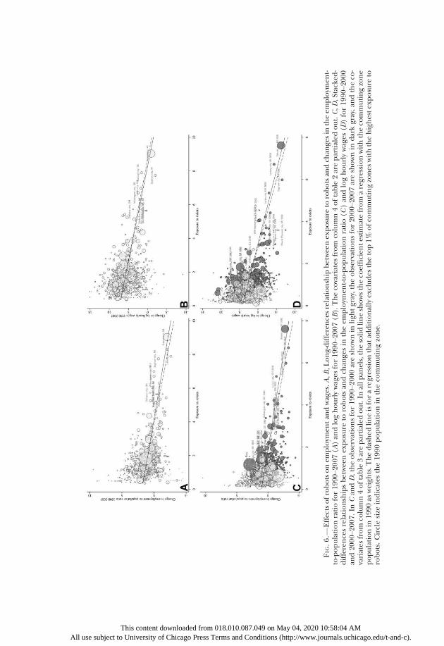
FIG

.6

.—E

ffec

tso

fro

bo

tso

nem

plo

ymen

tan

dw

ages

.A,B

,Lo

ng-

dif

fere

nce

sre

lati

on

ship

bet

wee

nex

po

sure

toro

bo

tsan

dch

ange

sin

the

emp

loym

ent-

to-p

op

ula

tio

nra

tio

for

1990

–20

07(A

)an

dlo

gh

ou

rly

wag

esfo

r19

90–20

07(B

).T

he

cova

riat

esfr

om

colu

mn

4o

fta

ble

2ar

ep

arti

aled

ou

t.C

,D,S

tack

ed-

dif

fere

nce

sre

lati

on

ship

sb

etw

een

exp

osu

reto

rob

ots

and

chan

ges

inth

eem

plo

ymen

t-to

-po

pu

lati

on

rati

o(C

)an

dlo

gh

ou

rly

wag

es(D

)fo

r19

90–20

00an

d20

00–20

07.

InC

andD

,th

eo

bse

rvat

ion

sfo

r19

90–20

00ar

esh

ow

nin

ligh

tgr

ay,

the

ob

serv

atio

ns

for

2000

–20

07ar

esh

ow

nin

dar

kgr

ay,

and

the

co-

vari

ates

fro

mco

lum

n4

of

tab

le3

are

par

tial

edo

ut.

Inal

lpan

els,

the

soli

dli

ne

sho

ws

the

coef

fici

ent

esti

mat

efr

om

are

gres

sio

nw

ith

the

com

mu

tin

gzo

ne

po

pu

lati

on

in19

90as

wei

ghts

.Th

ed

ash

edli

ne

isfo

ra

regr

essi

on

that

add

itio

nal

lyex

clu

des

the

top

1%o

fco

mm

uti

ng

zon

esw

ith

the

hig

hes

tex

po

sure

toro

bo

ts.

Cir

cle

size

ind

icat

esth

e19

90p

op

ula

tio

nin

the

com

mu

tin

gzo

ne.


robots and jobs 000

very large exposure to robots. Column 5 estimates the specification in col-umn 4 after excluding the top 1% of commuting zones with the highestexposure (which are the ones listed in n. 16) and demonstrates that thesehigh-exposure commuting zones are not driving our negative estimates.The coefficient estimate in panel A increases to20.57 (standard errors 50:14) and is shown with the dashed line in figure 6.

Finally, column 6 shows that the results are similar in unweighted re-gressions. In the same specification as in column 4, we now estimate a co-efficient of 20.51 (standard errors 5 0:12).

Panel B presents results for log hourly wages. Because wages are avail-able only for employed workers and our evidence in panel A suggests thatemployment declines in more exposed commuting zones, we present es-timates adjusted for changes in the composition of wage earners. Specif-ically, we use the change in the average log wage between 1990 and 2007for each of the 250 demographic cells in a commuting zone as our left-hand-side variable.21 Because we now have multiple observations for eachcommuting zone—one for each demographic group—we weight each ob-servation by the size of the demographic group in the commuting zone in1990. The estimates show that greater exposure to robots reduces wages.In column 4, when we control for our baseline covariates, the coefficientestimate is 20.88 (standard errors 5 0:13). This implies that a one-robotincrease in our exposure measure (per thousand workers) leads to 0.87%lower hourly wages. Figure 6 provides a residual regression plot for thisspecification as well.

We next turn to stacked-differences models, where we exploit variationover two periods: 1990–2000 and 2000–2007 (the former converted to a7-year equivalent change for consistency). In this case, our standard er-rors are robust against heteroskedasticity and within-state serial and spa-tial correlation. Table 3 presents our findings; panel A is for employmentand panel B for log hourly wages. Columns 1–6 have the same structure astable 2. In both panels, the estimates are more negative than before andremain precisely estimated. For example, in column 4 of panel A the co-efficient of interest is 20.55 (standard errors 5 0:05), while in panel Bthe estimate for log hourly wages increases to 21.4 (standard errors 50:18). Figure 6C and 6D illustrate these stacked-differences estimates, sep-arately marking observations from the two periods and showing that thenegative relationship is present in both periods.

The stacked-differences model focuses on the differential changes in ex-posure to robots between these two time periods and enables us to controlfor linear commuting zone trends. Although this specification is demand-ing and exploits a different source of variation than long differences, we

21 For each demographic group g in commuting zone c, we compute the long differenceof average log hourly wages Dln Wcg, as explained in n. 17. We then regress Dln Wcg on theexposure measure for commuting zone c and control for a full set of cell fixed effects.


This content downAll use subject to University of Ch

TA

BL

E3

EffectsofRobotsonEmploymentandWages:StackedDifferences

Stac

ked

Dif

fere

nce

s,19

90–20

00an

d20

00–20

07

Wei

ghte

db

yP

op

ula

tio

n

Exc

lud

esZ

on

esw

ith

Hig

hes

tE

xpo

sure

Un

wei

ghte

d

Co

mm

uti

ng

Zo

ne

Tre

nd

s

Wei

ghte

db

yP

op

ula

tio

n(7

)U

nw

eigh

ted

(8)

(1)

(2)

(3)

(4)

(5)

(6)

A.

Ch

ange

inE

mp

loym

ent-

to-P

op

ula

tio

nR

atio

,19

90–20

00an

d20

00–20

07

Exp

osu

reto

rob

ots

2.6

252

.591

2.5

252

.551

2.7

022

.743

2.5

082

1.00

7(.

092)

(.07

6)(.

059)

(.05

2)(.

150)

(.09

2)(.

079)

(.11

6)O

bse

rvat

ion

s1,

444

1,44

41,

444

1,44

41,

424

1,44

41,

444

1,44

4R

2.2

4.3

2.3

9.4

1.4

0.3

9.7

1.4

4

B.

Ch

ange

inL

og

Ho

url

yW

ages

,19

90–20

00an

d20

00–20

07

Exp

osu

reto

rob

ots

21.

544

21.

508

21.

405

21.

443

21.

643

21.

684

21.

608

22.

649

(.21

1)(.

199)

(.19

1)(.

182)

(.55

1)(.

295)

(.27

1)(.

407)

Ob

serv

atio

ns

183,

606

183,

606

183,

606

183,

606

180,

818

183,

606

183,

606

183,

606

R2

.28

.28

.28

.29

.27

.09

.32

.10

loaicag

dedo P

fre

000

rom 018.010ss Terms an

.0d

87Co

.049 ondition

n Ms (

ayhtt

04p:/

, 2/w

020 1ww.jo

0:5urn

8:0als

4 .uc

AMhic
ago .edu/t-and-c).

Co

vari

ates

Tim

ep

erio

dd

um

mie

s✓

✓✓

✓✓

✓✓

✓C

ensu

sd

ivis

ion

s✓

✓✓

✓✓

✓✓

✓D

emo

grap

hic

s✓

✓✓

✓✓

✓✓

Ind

ust

rysh

ares

✓✓

✓✓

✓✓

Tra

de,

rou

tin

ejo

bs

✓✓

✓✓

✓C

om

mu

tin

gzo

ne

tren

ds

✓✓

Note.—

Th

ista

ble

pre

sen

tses

tim

ates

of

the

effe

cts

of

exp

osu

reto

rob

ots

on

emp

loym

ent

and

wag

es.P

anel

Ap

rese

nts

stac

ked

-dif

fere

nce

ses

tim

ates

for

chan

ges

inth

eem

plo

ymen

t-to

-po

pu

lati

on

rati

ofo

r19

90–20

00an

d20

00–20

07.

Pan

elB

pre

sen

tsst

acke

d-d

iffe

ren

ces

esti

mat

esfo

rch

ange

sin

log

ho

url

yw

ages

for

1990

–20

00an

d20

00–20

07.

Th

esp

ecifi

cati

on

sin

pan

elB

are

esti

mat

edat

the

dem

ogr

aph

icce

ll�

com

mu

tin

gzo

ne

leve

l,w

her

ed

emo

grap

hic

cell

sar

ed

efin

edb

yag

e,ge

nd

er,e

du

cati

on

,an

dra

ce.C

olu

mn

s1–

5an

d7

pre

sen

tre

gres

sio

ns

wei

ghte

db

yp

op

ula

tio

nin

1990

.Co

lum

n5

pre

sen

tsre

sult

sex

clu

din

gth

eto

p1%

of

com

mu

tin

gzo

nes

wit

hth

eh

igh

est

exp

osu

reto

rob

ots

.Co

lum

ns

6an

d8

pre

sen

tu

nw

eigh

ted

regr

essi

on

s.T

he

cova

riat

esin

clu

ded

inea

chm

od

elar

ere

po

rted

atth

eb

ott

om

of

the

tab

le.

Co

lum

n1

incl

ud

eso

nly

cen

sus

div

isio

nd

um

mie

san

dti

me

per

iod

du

mm

ies.

Co

lum

n2

add

sd

e-m

ogr

aph

icch

arac

teri

stic

so

fco

mm

uti

ng

zon

es(l

og

po

pu

lati

on

;th

esh

are

of

fem

ales

;th

esh

are

of

the

po

pu

lati

on

ove

r65

year

so

ld;

the

shar

eso

fth

ep

op

ula

tio

nw

ith

no

coll

ege,

som

eco

lleg

e,co

lleg

eo

rp

rofe

ssio

nal

deg

ree,

and

mas

ters

or

do

cto

ral

deg

ree;

and

the

shar

eso

fw

hit

es,

bla

cks,

His

pan

ics,

and

Asi

ans)

.Co

lum

n3

add

sth

esh

ares

of

emp

loym

ent

inm

anu

fact

uri

ng

and

ligh

tm

anu

fact

uri

ng

and

the

fem

ale

shar

eo

fm

anu

fact

uri

ng

emp

loym

ent.

Co

lum

ns

4–6

add

exp

osu

reto

Ch

ines

eim

po

rts

and

the

shar

eo

fem

plo

ymen

tin

rou

tin

ejo

bs.

Inad

dit

ion

,co

ls.

7an

d8

incl

ud

ea

full

set

of

com

mu

tin

gzo

ne

fixe

def

fect

s.St

and

ard

erro

rsth

atar

ero

bu

stag

ain

sth

eter

osk

edas

tici

tyan

dco

rrel

atio

nw

ith

inst

ates

are

give

nin

par

enth

eses

.

A
ll use su bje ct T
to
hisUn
civ

oners

tenity

t d of

ow C

nlohic

adago

ed P

frores

0

ms T

00

01erm

8.010.087.049 on May 04, 2020 10:58:04 AMs and Conditions (http://www.journals.uchicago.edu/t-and-c).


All

estimate a similar negative impact of exposure to robots on both employ-ment and wages. In column 7, for example, the estimates for employ-ment and wages are, respectively, 20.5 (standard errors 5 0:08) and 21.6(standard errors 5 0:27). These findings bolster our confidence that ex-posed commuting zones are not simply on a differential trend unrelatedto advances in robotics technology. We also estimate negative employmentand wage effects of robot exposure for the entire period 1990–2014 as wellas for 2000–2007 and 2000–2014 (see table A13).

C. Other Labor Market Outcomes

In the appendix, we investigate the effects of exposure to robots on arange of other labor market outcomes. Table A14 shows robust negativeeffects on employment in manufacturing, which is relevant since robotsare mostly adopted in manufacturing and substitute directly for produc-tion workers in this industry.

Tables A15 and A16 look at alternative measures of employment andwages. These include the (private) employment-to-population ratio, in-cluding self-employment; the total employment-to-population ratio, in-cluding public employment and self-employment; employment countsfrom the CBP divided by population; log employment; log weekly wages;log yearly wages; and log wage bill from the CBP. The results are broadlysimilar to our baseline estimates in both long-differences and stacked-differences specifications for all of these measures.

Table A15 also explores the implications for nonemployment by lookingat the participation and unemployment margins. We estimate a positiveimpact of exposure to robots on the nonparticipation and unemploymentrates. Quantitatively, our estimates imply that about three-quarters of theadditional nonemployed drop out of the labor force, while one-quarter re-main unemployed. In line with the rise in nonparticipation, in table A17we also estimate increased use of Social Security Administration retirementand disability benefits and other government transfers.

Table A18 turns to the response of migration. Some of our estimatesshow a negative impact on population and net migration (computed fromthe IRS data), though these effects are neither consistent across specifica-tions nor precisely estimated. Quantitatively, the migration responses areabout one-quarter of the size of the employment responses.22 Consistentwith the spillovers on the nontradable sector that we report in section V.G,

22 For example, using our stacked-differences specification from col. 4 of table 3 andcomparing this to the equivalent specification in col. 4 of table A18 (panel D), we see thatan increase of one robot per thousand workers in our exposure measure reduces total em-ployment by 2%, of which 0.5% is explained by the decline in population and 1.5% is ex-plained by the decline in the employment-to-population ratio.


robots and jobs 000

table A18 also documents a decline in house prices and rents in exposedcommuting zones.

Finally, we use data from the BEA and the IRS to estimate the effects ofrobots on wage and nonwage income separately. Our estimates in table A19show precise and large negative effects on wage income and no significantimpact on nonwage income. This last result is consistent with the notionthat owners of robot integrators and firms introducing robotics technologyare not necessarily located in exposed commuting zones.

D. Threats to Validity

There are two main threats to the identifying assumption behind our esti-mates. First, the industries that have been adopting more robots over thelast two decades (in the United States and Europe) could have been on adownward trend because of declining demand, international competition,other technological changes, or worsening labor relations. Second, the com-muting zones that house the industries adopting more robots may be af-fected by other negative shocks. In either case, our estimates might con-found the impact of robots with these preexisting industry and commutingzone trends. (A third possible threat, that robot adoption is correlatedwith other concurrent technological changes, is discussed in the nextsubsection).

Our analysis in section IV, which demonstrates that the penetration ofrobots in EURO5 is not correlated with industry pretrends or with othermajor sources of changes in labor demand, is reassuring for the first threat.Moreover, the fact that value added has expanded in industries with thegreatest penetration of robots suggests that our measure is not correlatedwith negative demand shocks to industries. Regarding the second threat,our stacked-differences analysis, which controlled for commuting zonetrends, already established that linear commuting zone trends do not ex-plain our estimates. These results notwithstanding, we next investigatethese issues directly by checking for pretrends (which could result from ei-ther concern) and by controlling for other industry and commuting zonetrends.

Panel A of table 4 shows that there are no significant pretrends. Specifi-cally, we estimate the relationship between exposure to robots and changesin the employment-to-population ratio (cols. 1–4) and in log hourly wages(cols. 5–8) between 1970 and 1990. Our base specification, in columns 2and 6, shows that there is no quantitatively or statistically significant associ-ation between exposure to robots and pre-1990 changes in employment orwages. The picture is similar when we exclude highly exposed commutingzones in columns 3 and 7 and when we report unweighted specifications incolumns 4 and 8. These results are summarized in figure 7, which pres-ents residual plots for employment and wages from the specifications


This contentAll use subject to University

TA

BL

E4

EffectsofRobotsonEmploymentandWages:TestingandControllingforPretrends

Ch

ange

inE

mp

loym

ent-

to-P

op

ula

tio

nR

atio

Ch

ange

inL

og

Ho

url

yW

ages

Wei

ghte

db

yP

op

ula

tio

n

Exc

lud

esZ

on

esw

ith

Hig

hes

tE

xpo

sure

(3)

Un

wei

ghte

d(4

)

Wei

ghte

db

yP

op

ula

tio

n

Exc

lud

esZ

on

esw

ith

Hig

hes

tE

xpo

sure

(7)

Un

wei

ghte

d(8

)(1

)(2

)(5

)(6

)

A.

Pas

tC

han

gein

Lab

or

Mar

ket

Ou

tco

mes

,19

70–90

Exp

osu

reto

rob

ots

insu

bse

qu

ent

per

iod

,19

93–20

072

.014

.006

2.1

582

.217

.106

.145

.566

2.0

97(.

077)

(.07

0)(.

174)

(.15

1)(.

242)

(.24

3)(.

453)

(.35

9)O

bse

rvat

ion

s72

272

271

272

259

,230

59,2

3058

,402

59,2

30R

2.4

1.4

3.4

4.3

2.5

0.5

0.4

9.3

0

B.

Est

imat

esC

on

tro

llin

gfo

rE

xpo

sure

toIn

du

stry

Tre

nd

s,19

70–90

Exp

osu

reto

rob

ots

2.3

992

.411

2.4

922

.395

2.8

192

.824

2.6

142

.719

(.04

6)(.

049)

(.13

8)(.

100)

(.13

6)(.

135)

(.27

3)(.

226)

Exp

osu

reto

ind

ust

rytr

end

s19

70–90

2.0

412

.041

2.0

372

.063

2.0

652

.067

2.0

772

.115

(.01

9)(.

018)

(.01

9)(.

019)

(.03

4)(.

034)

(.03

4)(.

034)

Ob

serv

atio

ns

722

722

712

722

87,1

0087

,100

85,7

7687

,100

R2

.67

.67

.66

.63

.33

.33

.33

.08

dowof C

nhi

loaca

ded from 0go Press Te

0

1rm

00

8.0s

10.087and C

.0ond

49 iti

onons

M (h

ay ttp

04, 20://ww

20 w.j

10ou

:58rna

:04ls.u

Ach

Mica
go .edu/t-and-c).

C.

Est

imat

esC

on

tro

llin

gfo

rth

eC

han

gein

the

Dep

end

ent

Var

iab

le,

1970

–90

Exp

osu

reto

rob

ots

2.4

342

.449

2.5

872

.551

2.9

042

.913

2.7

892

1.15

7(.

057)

(.06

0)(.

132)

(.12

3)(.

144)

(.14

2)(.

291)

(.21

1)O

bse

rvat

ion

s72

272

271

272

255

,988

55,9

8855

,182

55,9

88R

2.6

6.6

7.6

6.6

2.4

1.4

1.4

0.1

6

Co

vari

ates

Cen

sus

div

isio

ns

✓✓

✓✓

✓✓

✓✓

Dem

ogr

aph

ics

and

ind

ust

rysh

ares

✓✓

✓✓

✓✓

✓✓

Tra

de,

rou

tin

ejo

bs

✓✓

✓✓

✓✓

Note.—

Th

ista

ble

pre

sen

tses

tim

ates

of

the

effe

cts

of

exp

osu

reto

rob

ots

on

pas

tem

plo

ymen

tan

dw

ages

,as

wel

las

esti

mat

eso

nco

nte

mp

ora

rych

ange

sin

emp

loym

ent

and

wag

esco

ntr

oll

ing

for

pas

tch

ange

sin

thes

eo

utc

om

es.P

anel

Ap

rese

nts

esti

mat

esfo

rch

ange

sin

the

emp

loym

ent-

to-p

op

ula

tio

nra

tio

(co

ls.1

–4)

and

log

ho

url

yw

ages

(co

ls.5

–8)

bet

wee

n19

70an

d19

90.F

or

com

par

iso

nw

ith

ou

rm

ain

resu

lts,

thes

eo

utc

om

esar

esc

aled

toa

14-y

ear

equ

iv-

alen

tch

ange

.Pan

elB

pre

sen

tslo

ng-

dif

fere

nce

ses

tim

ates

for

chan

ges

inth

eem

plo

ymen

t-to

-po

pu

lati

on

rati

o(c

ols

.1–4)

and

log

ho

url

yw

ages

(co

ls.5

–8)

bet

wee

n19

90an

d20

07co

ntr

oll

ing

for

am

easu

reo

fex

po

sure

toin

du

stri

esth

atw

ere

ind

ecli

ne

bet

wee

n19

70an

d19

90(s

eeth

em

ain

text

for

det

ails

on

this

vari

able

).P

anel

Cp

rese

nts

lon

g-d

iffe

ren

ces

esti

mat

esfo

rch

ange

sin

the

emp

loym

ent-

to-p

op

ula

tio

nra

tio

(co

ls.1

–4)

and

log

ho

url

yw

ages

(co

ls.5

–8)

bet

wee

n19

90an

d20

07co

ntr

oll

ing

for

the

chan

gein

the

dep

end

ent

vari

able

bet

wee

n19

70an

d19

90.

Th

esp

ecifi

cati

on

sfo

rlo

gh

ou

rly

wag

esar

ees

ti-

mat

edat

the

dem

ogr

aph

icce

ll�

com

mu

tin

gzo

ne

leve

l,w

her

ed

emo

grap

hic

cell

sar

ed

efin

edb

yag

e,ge

nd

er,e

du

cati

on

,an

dra

ce.C

olu

mn

s1–

3an

d5–

7p

rese

nt

regr

essi

on

sw

eigh

ted

by

po

pu

lati

on

in19

90.

Co

lum

ns

3an

d7

pre

sen

tre

sult

sex

clu

din

gth

eto

p1%

of

com

mu

tin

gzo

nes

wit

hh

igh

est

exp

osu

reto

rob

ots

.C

olu

mn

s4

and

8p

rese

nt

un

wei

ghte

dre

gres

sio

ns.

Th

eco

vari

ates

incl

ud

edin

each

mo

del

are

rep

ort

edat

the

bo

tto

mo

fth

eta

ble

.C

olu

mn

s1

and

5in

clu

de

cen

sus

div

isio

nd

um

mie

s,d

emo

grap

hic

char

acte

rist

ics

of

com

mu

tin

gzo

nes

(lo

gp

op

ula

tio

n;t

he

shar

eo

ffe

mal

es;t

he

shar

eo

fth

ep

op

ula

tio

no

ver

65ye

ars

old

;th

esh

ares

oft

he

po

pu

lati

on

wit

hn

oco

lleg

e,so

me

coll

ege,

coll

ege

or

pro

fess

ion

ald

egre

e,an

dm

aste

rso

rd

oct

ora

ldeg

ree;

and

the

shar

eso

fw

hit

es,b

lack

s,H

isp

anic

s,an

dA

sian

s),t

he

shar

eso

fem

plo

ymen

tin

man

ufa

ctu

rin

gan

dli

ghtm

anu

fact

uri

ng,

and

the

fem

ale

shar

eo

fman

ufa

ctu

rin

gem

plo

y-m

ent.

Inp

anel

A,t

he

bas

elin

eco

vari

ates

are

fro

m19

70,a

nd

inp

anel

sB

and

Cth

eyar

efr

om

1990

.Co

lum

ns

2–4

and

6–8

add

exp

osu

reto

Ch

ines

eim

po

rts

and

the

shar

eo

fem

plo

ymen

tin

rou

tin

ejo

bs.

Stan

dar

der

rors

that

are

rob

ust

agai

nst

het

ero

sked

asti

city

and

corr

elat

ion

wit

hin

stat

esar

egi

ven

inp

aren

thes

es.

A
ll use su bje Th
ct to U
is ni
cove

ntersit

nt y o

dof

w Ch

nloica

adego

d Pr

froess

00

m T

0

018erm

.0s

10.and

08 C

7.0on

49diti

onon

Ms (h

ay 04, 2020 10:58:04 AMttp://www.journals.uchicago.edu/t-and-c).


All

in columns 2, 3, 6, and 7. In table A20, we confirm that there are also nopretrends in other key labor market variables for which we have pre-1990data—in particular, manufacturing employment; the employment rate,including self-employment and the public sector; the nonparticipationrate; the unemployment rate; and log weekly wages.

FIG. 7.—Pretrends in employment and wages. This figure presents the relationship be-tween exposure to robots for 1993–2007 and the change in the employment-to-populationratio for 1970–1990 (A) and the change in log hourly wages for 1970–1990 (B). The covar-iates from column 2 of table 4 are partialed out. The solid line shows the coefficient estimatefrom a regression with the commuting zone population in 1990 as weights. The dashed lineis for a regression that additionally excludes the top 1% of commuting zones with highestexposure to robots. Circle size indicates the 1970 population in the commuting zone.


robots and jobs 000

Panel B of table 4 investigates potentially confounding industry trends.Specifically, we present estimates that control for predicted employmentdeclines based on a Bartik measure of exposure to industry trends in 1970–90. To construct this measure, we use the 19 IFR industries and interacttheir national log employment decline between 1970 and 1990 with theirbaseline employment share in 1970 in each commuting zone. Thoughthe coefficient of the Bartik measure for exposure to declining industrytrends is negative and significant in a few specifications, the point estimatesfor exposure to robots are unaffected. These results support our interpre-tation that the variable for exposure to robots is not proxying for decliningindustries.

Finally, panel C goes one step further and directly controls for the1970–90 change in the employment-to-population ratio or hourly wageson the right-hand side of our baseline specifications. This control has noeffect on our parameter estimates from table 2.

A related concern is that our estimates may have been driven or undulyinfluenced by the automotive industry, which adopted more robots thanany other sector between 1993 and 2007 and may be impacted by othereconomic trends.23

To address this concern, in table 5 we decompose our measure of expo-sure to robots into two parts, one exploiting the penetration of robots inthe automotive industry and the other exploiting the penetration of ro-bots in all other industries. We include both of these measures on theright-hand side of our employment and wage regressions. The table pres-ents both long-differences (cols. 1–3) and stacked-differences (cols. 4–6)specifications. Panel A is for employment, while panel B is for wages. Inboth panels, we find that the effects of exposure to robots in the automo-tive industry are similar to the effects of exposure to robots in other sec-tors. In none of these models do we reject the hypothesis that the coeffi-cients of these two variables are equal. These results are reassuring fortwo distinct reasons. First, they indicate that our results are not driven solelyby the automotive industry. Second, they also suggest that the effects of ro-bots in different sectors are broadly similar.

E. Robots, Capital, and Other Technologies

Our model demonstrates that capital deepening and technological changesthat do not automate tasks previously performed by labor do not generate a

23 Indeed, the share of employment in the automotive industry explains 67% of the cross-commuting zone variation in exposure to robots, and table A21 shows that the automotiveindustry has the highest Rotemberg weight, which ranges from 50% to 90% in the specifica-tions presented in table 2 (see Goldsmith-Pinkham, Sorkin, and Swift 2018). In our stacked-differences specifications in table 3, this industry also receives a large weight but only duringthe 2000–2007 period, when its robot penetration accelerated. These large Rotembergweights indicate that our reduced-form estimates may be sensitive to other shocks affectinglocal labor markets specializing in the automotive industry during this period.


All

TABLE 5Effects of Robots on Employment and Wages:

The Role of the Automotive Industry

Long Differences,1990–2007

Stacked Differences,1990–2000 and 2000–2007

Weighted byPopulation Un-

weighted(3)

Weighted byPopulation Un-

weighted(6)(1) (2) (4) (5)

A. Change in Employment-to-Population Ratio

Exposure to robots inautomotive industry 2.429 2.459 2.571 2.620 2.566 2.771

(.078) (.065) (.153) (.088) (.054) (.127)Exposure to robots in

other industries 2.505 2.370 2.451 2.654 2.449 2.695(.210) (.117) (.133) (.212) (.181) (.161)

Test for equality of co-efficients (p -value) .69 .42 .47 .87 .54 .72

Observations 722 722 722 1,444 1,444 1,444R 2 .27 .67 .62 .24 .41 .39

B. Change in Log Hourly Wages

Exposure to robots inautomotive industry 21.196 2.907 2.914 21.507 21.486 21.740

(.105) (.118) (.225) (.162) (.144) (.282)Exposure to robots in

other industries 21.314 2.715 2.955 21.740 21.144 21.588(.515) (.331) (.377) (.710) (.741) (.595)

Test for equality of co-efficients (p -value) .80 .52 .93 .73 .63 .81

Observations 87,100 87,100 87,100 183,606 183,606 183,606R 2 .32 .33 .08 .28 .29 .09

Covariates

Time period dummies ✓ ✓ ✓Census divisions ✓ ✓ ✓ ✓ ✓ ✓Baseline covariates ✓ ✓ ✓ ✓

This content use subject to University

downloaded from 018.010.087.049 oof Chicago Press Terms and Conditio

n May 04, 2020 10:58:ns (http://www.journal

Note.—This table presents estimates of the effects of exposure to robots separately forthe automotive industry and other industries. The p -value for a test of equality between thecoefficients of exposure to robots in the automotive industry and in other industries is re-ported below the estimates. Columns 1–3 present long-differences estimates for the 1990–2007 period. Columns 4–6 present stacked-differences estimates for the 1990–2000 and2000–2007 periods. Panel A presents results for the employment-to-population ratio. Panel Bpresents results for log hourly wages. The specifications in panel B are estimated at the de-mographic cell � commuting zone level, where demographic cells are defined by age, gen-der, education, and race. Columns 1, 2, 4, and 5 present regressions weighted by populationin 1990. Columns 3 and 6 present unweighted regressions. The covariates in each model arereported at the bottom of the table. Columns 1 and 4 include only census division dummies(and time period dummies in the stacked-differences specifications). Columns 2, 3, 5, and 6add demographic characteristics of commuting zones (log population; the share of females;the share of the population over 65 years old; the shares of the population with no college,some college, college or professional degree, and masters or doctoral degree; and theshares of whites, blacks, Hispanics, and Asians), the shares of employment in manufacturingand light manufacturing, the female share of manufacturing employment, exposure to Chi-nese imports, and the share of employment in routine jobs. Standard errors that are robustagainst heteroskedasticity and correlation within states are given in parentheses.

04 AMs.uchicago.edu/t-and-c).

robots and jobs 000

displacement effect and should thus have very different impacts on labordemand. We now investigate the effects of capital deepening, increases inITcapital, and growth in value added on employment and wages. We wantto understand whether the effects of these variables differ from the effectsof robots and also verify that controlling for these trends does not changeour main estimates.

Table 6 presents the results from this exercise. We again report bothlong-differences and stacked-differences specifications. Columns 1–4are for employment, while columns 5–8 are for wages. In panel A, we con-trol for exposure to capital, which is a Bartik measure of the increase in(log) industry capital stocks. In panels B and C, we control for exposureto ITcapital and exposure to industry value added (which are Bartik mea-sures of increases in log industry ITcapital and in log industry value added,respectively).

Including these variables has little effect on our estimates of the impactof robots. Moreover, and in line with our theoretical emphasis that auto-mation is conceptually different from capital deepening and other typesof technological changes that increase value added, these variables are, ifanything, positively correlated with changes in employment and wages(see table A23 for broadly similar results with other measures of computertechnology). These results confirm our expectation that, due to the dis-placement effect, industrial robots should have a very different impacton labor demand than other (nonautomation) technologies. They alsobolster the case that our estimates are not capturing the effects of otherconcurrent technological changes (since these tend to have different im-pacts from robots and, as already shown in table A3, are uncorrelated withexposure to robots).24

F. Other Robustness Checks

The appendix reports a range of additional robustness checks. First, ta-bles A24 and A25 show that the exact construction of exposure to robotsdoes not affect our results. We report estimates where this measure iscomputed from the average of all European countries and from the aver-age of EURO5 plus Germany, as well as a specification where we use the1990 (rather than the 1970) employment distribution. In addition, we

24 Another related threat to our IV strategy is that, as noted in n. 3, international compe-tition may affect robot adoption decisions in both the United States and Europe. Relatedly,investments in robots in the countries that are most advanced in robotics technology—Ger-many, Japan, and South Korea—may increase international competition for US industries.Table A22 investigates these issues and shows that our estimates of the effects of robots aresimilar when we control for exposure to imports from Mexico, task offshoring, and exportsfrom Germany, Japan, and South Korea.


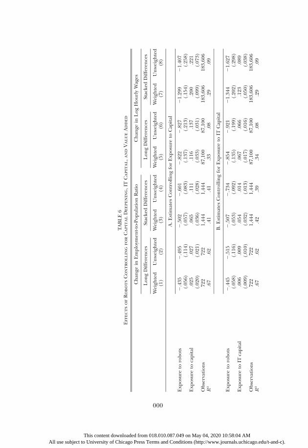
TA

BL

E6

EffectsofRobotsControllingforCapitalDeepening,ITCapital,andValueAdded

Ch

ange

inE

mp

loym

ent-

to-P

op

ula

tio

nR

atio

Ch

ange

inL

og

Ho

url

yW

ages

Lo

ng

Dif

fere

nce

sSt

acke

dD

iffe

ren

ces

Lo

ng

Dif

fere

nce

sSt

acke

dD

iffe

ren

ces

Wei

ghte

d(1

)U

nw

eigh

ted

(2)

Wei

ghte

d(3

)U

nw

eigh

ted

(4)

Wei

ghte

d(5

)U

nw

eigh

ted

(6)

Wei

ghte

d(7

)U

nw

eigh

ted

(8)

A.

Est

imat

esC

on

tro

llin

gfo

rE

xpo

sure

toC

apit

al

Exp

osu

reto

rob

ots

2.4

352

.495

2.5

022

.601

2.8

222

.827

21.

299

21.

407

(.05

6)(.

114)

(.05

7)(.

083)

(.13

7)(.

213)

(.15

4)(.

258)

Exp

osu

reto

cap

ital

.025

.027

.065

.111

.116

.137

.200

.221

(.02

0)(.

021)

(.03

6)(.

028)

(.03

3)(.

031)

(.09

9)(.

073)

Ob

serv

atio

ns

722

722

1,44

41,

444

87,1

0087

,100

183,

606

183,

606

R2

.67

.62

.41

.41

.33

.08

.29

.09

B.

Est

imat

esC

on

tro

llin

gfo

rE

xpo

sure

toIT

Cap

ital

Exp

osu

reto

rob

ots

2.4

452

.515

2.5

072

.734

2.8

542

.921

21.

344

21.

627

(.05

8)(.

116)

(.05

3)(.

092)

(.13

5)(.

199)

(.20

2)(.

298)

Exp

osu

reto

ITca

pit

al.0

06.0

09.0

54.0

14.0

67.0

66.1

23.0

89(.

009)

(.01

0)(.

032)

(.01

3)(.

017)

(.01

6)(.

050)

(.03

8)O

bse

rvat

ion

s72

272

21,

444

1,44

487

,100

87,1

0018

3,60

618

3,60

6R

2.6

7.6

2.4

2.3

9.3

4.0

8.2

9.0

9

000


TA

BL

E6

(CONTIN

UED

)

Ch

ange

inE

mp

loym

ent-

to-P

op

ula

tio

nR

atio

Ch

ange

inL

og

Ho

url

yW

ages

Lo

ng

Dif

fere

nce

sSt

acke

dD

iffe

ren

ces

Lo

ng

Dif

fere

nce

sSt

acke

dD

iffe

ren

ces

Wei

ghte

d(1

)U

nw

eigh

ted

(2)

Wei

ghte

d(3

)U

nw

eigh

ted

(4)

Wei

ghte

d(5

)U

nw

eigh

ted

(6)

Wei

ghte

d(7

)U

nw

eigh

ted

(8)

C.

Est

imat

esC

on

tro

llin

gfo

rE

xpo

sure

toIn

du

stry

Val

ue

Ad

ded

Exp

osu

reto

rob

ots

2.4

832

.563

2.5

882

.782

2.9

032

.958

21.

487

21.

717

(.06

1)(.

113)

(.05

1)(.

087)

(.13

3)(.

201)

(.18

3)(.

292)

Exp

osu

reto

ind

ust

ryva

lue

add

ed.0

60.0

64.0

82.0

79.0

34.0

33.0

97.0

62(.

013)

(.01

5)(.

024)

(.01

8)(.

021)

(.01

7)(.

054)

(.02

5)O

bse

rvat

ion

s72

272

21,

444

1,44

487

,100

87,1

0018

3,60

618

3,60

6R

2.6

9.6

4.4

2.4

1.3

3.0

8.2

9.0

9

Co

vari

ates

Tim

ep

erio

dd

um

mie

s✓

✓✓

✓C

ensu

sd

ivis

ion

san

db

asel

ine

cova

riat

es✓

✓✓

✓✓

✓✓

✓

Note.—

Th

ista

ble

pre

sen

tses

tim

ates

of

the

effe

cts

of

exp

osu

reto

rob

ots

,cap

ital

accu

mu

lati

on

,IT

cap

ital

,an

dva

lue

add

edo

nem

plo

ymen

tan

dw

ages

.C

olu

mn

s1,

2,5,

and

6p

rese

nt

lon

g-d

iffe

ren

ces

esti

mat

esfo

r19

90–20

07.C

olu

mn

s3,

4,7,

and

8p

rese

nt

stac

ked

-dif

fere

nce

ses

tim

ates

for

1990

–20

00an

d20

00–20

07.C

olu

mn

s1–

4p

rese

nt

resu

lts

for

the

emp

loym

ent-

to-p

op

ula

tio

nra

tio

.Co

lum

ns

5–8

pre

sen

tre

sult

sfo

rlo

gh

ou

rly

wag

es.T

he

spec

ifica

tio

ns

inco

ls.

5–8

for

log

ho

url

yw

ages

are

esti

mat

edat

the

dem

ogr

aph

icce

ll�

com

mu

tin

gzo

ne

leve

l,w

her

ed

emo

grap

hic

cell

sar

ed

efin

edb

yag

e,ge

nd

er,

ed-

uca

tio

n,

and

race

.O

dd

-nu

mb

ered

colu

mn

sp

rese

nt

regr

essi

on

sw

eigh

ted

by

po

pu

lati

on

in19

90.

Eve

n-n

um

ber

edco

lum

ns

pre

sen

tu

nw

eigh

ted

regr

es-

sio

ns.

Inp

anel

A,

we

con

tro

lfo

ra

mea

sure

of

exp

osu

reto

cap

ital

,co

nst

ruct

edb

yin

tera

ctin

gth

ein

crea

sein

log

cap

ital

inea

chin

du

stry

wit

hit

sb

asel

ine

emp

loym

ent

shar

ein

the

com

mu

tin

gzo

ne.

Inp

anel

B,w

eco

ntr

olf

or

am

easu

reo

fex

po

sure

toIT

cap

ital

,co

nst

ruct

edb

yin

tera

ctin

gth

ein

crea

sein

log

ITca

pit

alin

each

ind

ust

ryw

ith

its

bas

elin

eem

plo

ymen

tsh

are

inth

eco

mm

uti

ng

zon

e.In

pan

elC

,w

eco

ntr

ol

for

am

easu

reo

fex

po

sure

toin

du

stry

valu

ead

ded

,co

nst

ruct

edb

yin

tera

ctin

gth

ein

crea

sein

log

valu

ead

ded

inea

chin

du

stry

(bet

wee

n19

92an

d20

07in

all

mo

del

s)w

ith

its

bas

elin

eem

plo

ymen

tsh

are

inth

eco

mm

uti

ng

zon

e.A

llm

od

els

incl

ud

ece

nsu

sd

ivis

ion

du

mm

ies

(an

dti

me

per

iod

du

mm

ies

inth

est

acke

d-d

iffe

ren

ces

spec

ifica

tio

ns)

,d

emo

-gr

aph

icch

arac

teri

stic

so

fco

mm

uti

ng

zon

es(l

og

po

pu

lati

on

;th

esh

are

of

fem

ales

;th

esh

are

of

the

po

pu

lati

on

ove

r65

year

so

ld;

the

shar

eso

fth

ep

op

-u

lati

on

wit

hn

oco

lleg

e,so

me

coll

ege,

coll

ege

or

pro

fess

ion

ald

egre

e,an

dm

aste

rso

rd

oct

ora

ld

egre

e;an

dth

esh

ares

of

wh

ites

,b

lack

s,H

isp

anic

s,an

dA

sian

s),t

he

shar

eso

fem

plo

ymen

tin

man

ufa

ctu

rin

gan

dli

ght

man

ufa

ctu

rin

g,th

efe

mal

esh

are

of

man

ufa

ctu

rin

gem

plo

ymen

t,ex

po

sure

toC

hin

ese

im-

po

rts,

and

the

shar

eo

fem

plo

ymen

tin

rou

tin

ejo

bs.

Stan

dar

der

rors

that

are

rob

ust

agai

nst

het

ero

sked

asti

city

and

corr

elat

ion

wit

hin

stat

esar

egi

ven

inp

aren

thes

es.

000



All

present estimates for an exposure measure based on the raw penetrationof robots (rather than our theoretically grounded measure based on ad-justed penetration of robots) and from a specification where we weighteach industry’s adjusted penetration of robots by the average cost of ro-bots in that industry. In all cases, the reduced-form estimates using thesealternative measures of exposure are negative and significant (and the IVestimates reported in col. 7 of tables A24 and A25 are also similar to theestimates in table 7 presented in the next section).

Table A26 explores the role of outliers. Our results are robust when weexclude Detroit (the commuting zone with the highest exposure to ro-bots); when we exclude observations with residuals above or below 1.95standard deviations; when we estimate Li’s (1985) robust regression,which downweights influential observations; and when we estimate me-dian regressions.

Table A27 shows that our results are also robust to controlling for a fullset of state fixed effects, to allowing for mean-reverting dynamics in em-ployment and wages by including the baseline value of the dependent var-iable, and to controlling for contemporaneous changes in all of our base-line demographic variables. Table A28 reports the results from a two-stepleast absolute shrinkage and selection operator (LASSO) specification witha large number of covariates (following Belloni, Chernozhukov, and Han-sen 2014) and establishes that those included in our main specificationsare very similar to those identified by the LASSO procedure, and the two-step estimates are close to our baseline estimates.

G. Effects by Industry, Occupation, Gender, and Skill

This subsection investigates how exposure to robots has affected employ-ment in different industries and occupations as well as the employmentand wages of different workers.

Figure 8A presents estimates of the effects of exposure to robots onemployment in different industries. We present point estimates and con-fidence intervals for two long-differences specifications analogous to col-umns 4 and 5 of table 2 and one stacked-differences specification corre-sponding to column 4 of table 3 (fig. A4 presents estimates from analogousunweighted specifications). Figure 8 shows that the effects of robots con-centrate in manufacturing (also shown in table A14) and especially in heav-ily robotized industries, which include automotive, plastics and chemicals,metal products, basic metals, electronics, and food and beverages. Thereare no significant effects on the remaining manufacturing industries. Con-sistent with the indirect effects on nontradables discussed in section II.B,we find negative impacts on construction and retail and personal services.The only two sectors that show positive effects in some specifications are(1) agriculture and education and (2) health care and the public sector (al-though these estimates are neither precise nor robust).


TABLE 7Effects of Robots on Employment and Wages: IV Estimates

Change in Employment-to-Population Ratio Change in Log Hourly Wages

(1) (2) (3) (4) (5) (6)

A. Long Differences, 1990–2007

US exposure to robots 2.375 2.377 2.388 21.022 2.762 2.768(.119) (.088) (.091) (.225) (.147) (.148)

Observations 722 722 722 87,100 87,100 87,100First-stage coefficient 1.19 1.15 1.15 1.19 1.15 1.15First-stage F-statistic 38.16 32.19 33.62 39.81 33.17 34.35

B. Alternative Imputation of US Data, 1990–2007


Observations 722 722 722 87,100 87,100 87,100First-stage coefficient 1.15 1.11 1.11 1.15 1.11 1.11First-stage F -statistic 38.16 32.19 33.62 39.81 33.17 34.35

C. Long Differences, 1990–2014


Observations 722 722 722 90,341 90,341 90,341First-stage coefficient 1.20 1.14 1.15 1.21 1.14 1.15First-stage F -statistic 105.01 68.75 73.34 110.32 70.35 74.86

D. Long Differences, 2000–2007


Observations 722 722 722 99,319 99,319 99,319First-stage coefficient .79 .76 .75 .79 .76 .75First-stage F -statistic 211.46 123.73 124.32 223.26 131.40 131.83

E. Long Differences, 2000–2014


Observations 722 722 722 106,375 106,375 106,375First-stage coefficient 1.00 .92 .93 1.00 .92 .93First-stage F -statistic 1,195.67 305.25 298.98 1,296.85 324.38 316.40

Covariates

Division dummies ✓ ✓ ✓ ✓ ✓ ✓Demographics and industry shares ✓ ✓ ✓ ✓Trade, routine jobs ✓ ✓

This content doAll use subject to University of

wnloaded from 018.010.087.04Chicago Press Terms and Cond

9 on May 04itions (http://

, 2020 10:5www.journ

Note.—This table presents IV estimates of the effects of exposure to robots on employ-ment and wages for different time periods. Panels A and B present results for 1990–2007.Panel C presents results for 1990–2014. Panel D presents results for 2000–2007. Panel Epresents results for 2000–2014. In all models, we instrument the US exposure to robots us-ing exposure to robots from EURO5. In panels A and C–E, we rescale the US exposure torobots to match the time period used. In panel B, we use an alternative imputation strategyfor US exposure to robots described in the main text. Columns 1–3 present results for theemployment-to-population ratio. Columns 4–6 present results for log hourly wages. Thespecifications for log hourly wages are estimated at the demographic cell � commutingzone level, where demographic cells are defined by age, gender, education, and race. AllIV estimates are from regressions weighted by population in 1990. The covariates includedin each model are reported at the bottom of the table. Columns 1 and 4 include only censusdivision dummies. Columns 2 and 5 add demographic characteristics of commuting zones(log population; the share of females; the share of the population over 65 years old; theshares of the population with no college, some college, college or professional degree,and masters or doctoral degree; and the shares of whites, blacks, Hispanics, and Asians),the shares of employment in manufacturing and light manufacturing, and the female shareof manufacturing employment. Columns 3 and 6 add exposure to Chinese imports and theshare of employment in routine jobs. We also report the first-stage coefficients and their F-statistics in all models. Standard errors that are robust against heteroskedasticity and corre-lation within states are given in parentheses.

8:04 AMals.uchicago.edu/t-and-c).


All

Figure 8B presents analogous results for employment by occupation.In line with our expectations, the negative employment effects of robotsare mostly in routine manual occupations and particularly in blue-collaroccupations, such as machinists, assemblers, material handlers, andwelders. Workers in these occupations engage in tasks that are being au-tomated by industrial robots, so it is natural for them to experience thebulk of the displacement effect created by robots. We do not estimate pos-itive employment effects in other occupations, suggesting that, at least lo-cally, the productivity gains from using industrial robots have not resultedin an expansion of employment in nonautomated tasks.

Figure 9 and table A29 investigate the employment and wage effects bygender. We estimate negative impacts for both men and women. The ef-fects are larger for men. For example, with our baseline specification inlong differences, reported in figure 9 and in column 1 of table A29, the im-pact of exposure to robots on the employment-to-population ratio of menis 20.57, while for women it is 20.34. Table A29 further shows that the de-cline for male employment is concentrated in manufacturing, while thedecline in female employment is more pronounced in nonmanufacturing.

Figure 9 summarizes the effects of robots on employment and wagesfor workers in different education groups. We present estimates for allworkers and estimates for men and for women separately. We see negativeemployment and wage effects for both men and women with less thanhigh school, high school degree, some college, and college or professionaldegree. We find it surprising that there is no positive effect on workerswith a masters or doctoral degree. One interpretation is that this result re-flects reduced demand for these workers from the nontradable sector. Acomplementary explanation is that, in contrast to other computer-assistedtechnologies, industrial robots are not directly complementing high-skillworkers. Figure 10 investigates the impact of exposure to robots on thewage distribution by estimating quantile regressions (using our baselinespecification from col. 4 of table 2). For all workers, we estimate negativeand significant effects below the 35th percentile of the wage distribution.When we focus on workers with no college degree, the negative and sig-nificant effects extend all the way to the 85th percentile, while for workerswith a college degree or more, the negative effects concentrate below the15th percentile. These results confirm that the negative wage effects ofrobots are mostly at the bottom and the middle of the distribution.

VI. IV Estimates and Local and AggregateImplications

In this section, we report our IV estimates and explore their quantitativeimplications for local and aggregate changes in employment and wages.


FIG

.8

.—E

ffec

tso

fro

bo

tso

nin

du

stri

esan

do

ccu

pat

ion

s.T

his

figu

rep

rese

nts

esti

mat

eso

fth

eef

fect

so

fex

po

sure

toro

bo

tso

nch

ange

sin

ind

ust

ryem

plo

ymen

t-to

-po

pu

lati

on

rati

os

(A)

and

chan

ges

ino

ccu

pat

ion

emp

loym

ent-

to-p

op

ula

tio

nra

tio

s(B

).T

he

cap

ped

lin

esp

rovi

de

95%

con

fid

ence

inte

r-va

ls.

Th

efi

rst

set

of

esti

mat

esar

efr

om

lon

g-d

iffe

ren

ces

spec

ifica

tio

ns

asin

colu

mn

4o

fta

ble

2.T

he

seco

nd

set

of

esti

mat

esar

efr

om

lon

g-d

iffe

ren

ces

spec

ifica

tio

ns

asin

colu

mn

5o

fta

ble

2(w

her

ew

ere

mo

veth

eto

p1%

of

com

mu

tin

gzo

nes

wit

hth

eh

igh

est

exp

osu

reto

rob

ots

).T

he

thir

dse

to

fes

tim

ates

are

fro

mst

acke

d-d

iffe

ren

ces

spec

ifica

tio

ns

asin

colu

mn

4o

fta

ble

3.


FIG

.9

.—E

ffec

tso

fro

bo

tso

nem

plo

ymen

tan

dw

ages

by

edu

cati

on

and

gen

der

.Th

isfi

gure

pre

sen

tses

tim

ates

oft

he

effe

cts

ofe

xpo

sure

toro

bo

tso

nch

ange

sin

the

emp

loym

ent-t

o-p

op

ula

tio

nra

tio

(A)

and

chan

gesi

nlo

gh

ou

rly

wag

es(B

)fo

ral

lwo

rker

san

dfo

rm

enan

dw

om

enw

ith

dif

fere

nte

du

cati

on

leve

ls(l

esst

han

hig

hsc

ho

ol,

hig

hsc

ho

old

egre

e,so

me

colle

ge,c

olle

geo

rp

rofe

ssio

nal

deg

ree,

and

mas

ters

or

do

cto

rald

egre

e).T

he

cap

ped

lines

pro

vid

e95

%co

nfi

den

cein

terv

als.


robots and jobs 000

A. IV Estimates

We use the US exposure to robots to compute two-stage least squares(2SLS) estimates of bL and bW in equation (13). Figure 2 already showedthe close association between the industry-level spread of robots in theUnited States (APRi,(2004,2007)) and in Europe (APRi,ð1993,2007Þ). Figure A3 de-picts our first-stage relationship by plotting the US exposure to robots atthe commuting zone level computed usingAPRi,(2004,2007) against exposureto robots computed using APRi,ð1993,2007Þ.

Table 7 reports our IV estimates for the long-differences specificationsanalogous to those in table 2 and also reports the corresponding first-stage coefficients and F -statistics (table A33 reports the corresponding

FIG. 10.—Effects of robots on the wage distribution. This figure presents estimates of theeffects of exposure to robots on quantiles of the wage distribution for a specification equiv-alent to column 4 in table 2, following the methodology of Chetverikov, Larsen, and Palmer(2016). Estimates for the 5th, 10th, . . . , and 95th quantiles together with their 95% confi-dence intervals are shown. The different panels are for all workers (A), for workers with nocollege degree (B), and for workers with a college degree or more (C) separately and formen (D) and women (E) separately.



All

OLS estimates). Because we use the IVestimates to quantify the aggregateimplications of robot adoption, we focus on the population-weightedspecifications. Columns 1–3 are for the (private) employment-to-populationratio, and columns 4–6 are for log hourly wages. Column 1 in each panelpresents a parsimonious specification that controls only for census divi-sion dummies. Column 2 in each panel additionally controls for demo-graphic characteristics and industry composition of commuting zones. Fi-nally, column 3 in each panel adds controls for imports from China andthe decline of routine jobs.

Panel A covers our baseline period, 1990–2007, where the 2004–7 USdata are rescaled to a 14-year equivalent change. Panel B also focuses on1990–2007 but constructs the US exposure to robots by imputing US in-dustry data using the aggregate US change between 1993 and 2004 ratherthan rescaling the 2004–7 industry data. Panel C is for 1990–2014, whilepanels D and E focus on 2000–2007 and 2000–2014, respectively, timewindows that closely overlap with US robots data. In all cases, the 2SLS es-timates are negative and precise for both employment and wages. Our baseestimates in columns 3 and 6 in panel A, which we use in our quantitativeevaluation in the next subsection, are 20.39 (standard errors 5 0:09) foremployment and 20.77 (standard errors 5 0:15) for log hourly wages.25

The estimates in table 7 present standard errors that are robust againstheteroskedasticity and within-state spatial correlation. As pointed out byBorusyak, Hull, and Jaravel (2018), these standard errors do not take intoaccount potential correlations across commuting zones resulting fromother industry shocks. Table A20 reproduces our IV estimates with stan-dard errors computed following Borusyak et al.’s (2018) procedure to ac-count for such correlation (tables A31 and A32 present these adjustedstandard errors for our main long- and stacked-differences reduced-formmodels). We do not find systematic differences between our baseline stan-dard errors and these potentially more conservative standard errors, pre-sumably because our specifications already control for the most importantindustry shocks affecting US labor markets, such as import competitionfrom China, trends in overall manufacturing, light manufacturing, and thedecline of routine jobs.

B. Magnitudes

The IV estimates in the previous subsection quantify the impact of im-provements in automation technologies that lead to the adoption of oneadditional robot per thousand workers on employment and wages in a

25 For 1990–2014 in panel C, the IV estimate for employment is 40% smaller and the es-timate for wages is 40% larger. This might reflect the fact that as wages have continued toadjust in the affected commuting zones, some of the initial employment response may havebeen reversed.


robots and jobs 000

commuting zone relative to other areas. Our estimates in columns 3 and6 in panel A, for example, imply that the adoption of one additional ro-bot per thousand workers in a commuting zone reduces its employment-to-population ratio by 0.39 percentage points (roughly a 1% decline) andhourly wages by 0.77% relative to other commuting zones. These num-bers suggest that one more robot reduces employment by about six work-ers in the affected commuting zone relative to others.26 These are sizablemagnitudes but are not implausible since they include both the direct ef-fects of robots on employment and wages and the spillover effects on non-tradables resulting from the decline in local demand following the loss ofemployment and wage income in the area we saw in section V.G.27

The more challenging question is how much (and whether) employ-ment and wages in the aggregate decline in response to the adoptionof industrial robots. As emphasized in proposition 3, when commutingzones interact through trade and capital markets, our local IV estimatesdo not directly translate into aggregate effects because robot adoption inone commuting zone reduces the costs of goods consumed in other areasand generates capital income gains shared by households across the UnitedStates. To explore these aggregate implications, we need to make furtherassumptions on cross-commuting zone spillovers (and this suggests greatercaution in interpreting these aggregate estimates than the local effects dis-cussed in the previous paragraph).

We first assume that proposition 3 provides a reliable approximation tothese cross-commuting zone interactions and use our regression evidenceand external information to discipline the key parameters of the model.Specifically, we use equations (9) and (10) in proposition 3, which provideexpressions for bL and bW in terms of the underlying parameters of themodel as well as the factor shares. We then use information on factorshares and j, l, a, p0, and gM=gL to solve for the values of the inverse ofthe wage elasticity of labor supply, ε, and the inverse of the elasticity of therobot supply, h, that are consistent with our IV estimates, b̂L and b̂W . With

26 The increase of one more robot per thousand workers between 1993 and 2007 isequivalent to an increase of 0.6 robots per thousand people or a total increase of120,000 robots. Our estimates imply that these additional robots led to a 0.39 percentagepoints lower (private) employment-to-population ratio, which is equivalent to one robotreducing employment by six (≈0:0039=ð0:6=1,000Þ) workers. Equivalently, the increaseof 120,000 in the stock of robots during this period is predicted to have reduced employ-ment by 756,000 jobs. We obtain a reduction in employment of 720,000 jobs (or about fourjobs per robot) if we use the estimate for 1990–2014 from panel C together with the largerincrease of 180,000 in the stock of robots over this longer time period.

27 These magnitudes can be compared to the local effects from exposure to importsfrom China. Using the stacked-differences estimates from table A12, which correspondto the specification used in Autor, Dorn, and Hanson (2013), the implied magnitude fromthe rise in Chinese imports is a decline of about 1 percentage point in the employment-to-population ratio—2.5 times the 0.39 percentage points decline due to the rising use of in-dustrial robots.



All

these parameter estimates, we compute the aggregate implications of ro-bots from our model. Proposition A7 in the appendix provides formulaslinking the aggregate effects of robots on employment and wages to theparameters h and ε.

Our parameter choices are as follows: (1) j 5 1 as the elasticity of sub-stitution between different industries (see Oberfield and Raval 2014);(2) l 5 5 for the elasticity of substitution between traded varieties, whichfollows the trade literature (e.g., Head and Meyer 2014; Simonovska andWaugh 2014); (3) sL 5 0:9916 as the baseline share of labor in task pro-duction, which is implied by the number of robots in US industries in1993;28 (4) a 5 0:67, which together with the estimate for sL yields an ini-tial labor share of approximately two-thirds in all commuting zones;(5) f 5 0:25, which matches the 18% share of employment in the trad-able or manufacturing sector; (6) p0 5 0:3, which, in line with the evi-dence surveyed in BCG (2015), implies that robot adoption reduces costsby about 30%; (7) gM=gL 5 3, which implies that in automated tasks a ro-bot performs on average the work of three workers;29 and (8) w 5 0:02,which is consistent with a marginal propensity to consume leisure of10% (see Imbens, Rubin, and Sacerdote 2001).

Given these parameter values, equations (9) and (10) yield h 5 0:79and ε 5 0:17. The estimate for h implies a fairly inelastic supply of robotsto the local economy, which limits the productivity gains from robot adop-tion and instead generates greater rents for robot integrators and produc-ers. If we suppose that local robot services are provided by combining(elastically supplied) robotics equipment and (mostly inelastically) sup-plied services of robot integrators, this estimate is equivalent to the shareof the inelastic component of integrators’ services, h=ð1 1 hÞ, being ap-proximately 0.44. Since the share of local robot integrators in total costsis about 0.75 (Leigh and Kraft 2018), this number implies that abouttwo-thirds of their services are inelastically supplied to the local economy.The estimate for ε, on the other hand, implies an elastic response of laborsupply. This estimate is in line with the “macro” Frisch elasticities that are

28 In propositions 2 and 3, we simplified the exposition by focusing on the case wherev0 5 0, which implied a share of labor in task production equal to sL 5 1. Our more gen-eral expressions in propositions A2 and A6 clarify the role of sL.

29 This number is consistent with both the conclusions of the early engineering studieson the capabilities of industrial robots (see Groover et al. 1986) and more recent estimates.For example, Ford (2015, 2) reports that robots can move six times as many boxes as hu-mans in the same time period. Robots also appear to be three times as productive in weld-ing as humans (see https://www.sciencechannel.com/tv-shows/worlds-biggest-shipbuilders),six times as productive in placing bricks (see https://www.cnbc.com/2018/02/17/construction-robotics-bricklaying-robot-five-times-faster-than-human.html), and nine times as productivein smartphone assembly (see https://futurism.com/2-production-soars-for-chinese-factory-who-replaced-90-of-employees-with-robots).


robots and jobs 000

consistent with the observed short-run movements in wages and employ-ment (see table 1 in Chetty et al. 2011).

Using these parameter estimates, we compute the aggregate effects ofimprovements in robotics technology. One more robot per thousand work-ers is predicted to reduce aggregate wages by 0.42% and the aggregateemployment-to-population ratio by 0.2 percentage points (or 400,000jobs); equivalently, one more robot reduces employment by 3.3 work-ers.30 With these parameter values, about two-thirds of the decline inthe demand for labor in an exposed commuting zone is driven by thecontraction of the nontradable sector. This estimate is consistent withthe magnitudes of the decline in employment in nontradables, such as con-struction, retail, and personal services, documented in section V.G (wheremanufacturing accounts for 0.16 of the 0.45 decline in the employment-to-population ratio in response to one more robot per thousand workers,with the rest of the decline accounted for by nontradables). Our model alsoimplies a 0.33% increase in the productivity of the tradable sector, a sizablecapital income gain of 1.87%, and a 136% increase in industrial robot uti-lization. This last estimate closely matches the 139% increase in the stock ofrobots observed during this period.

Table A34 considers variations in the values of the key parameters, j, l,p0, gM=gL, and w, and shows that both the implied values of h and ε and theresulting aggregate effects are not very sensitive to reasonable variations.

VII. Concluding Remarks

The spread of robots, artificial intelligence, and other automation tech-nologies has raised concerns about the future of jobs and wages. Never-theless, there has been relatively little work on the equilibrium effectsof new automation technologies and particularly of robots. In this paper,we investigate the effects of industrial robots on US local labor markets.Robots—and automation technologies more generally—displace work-ers from tasks that they were previously performing and should thus havevery different labor market effects than overall capital deepening andother types of technological changes (such as factor-augmenting ones).This is what we find in our empirical work.

We focus on the variation in robot adoption originating from the tech-nological frontier, proxied by trends in other economies that are more ad-vanced than the United States in robotics technology (which are ahead of

30 The aggregate effects are broadly similar if we use the IV estimate for 1990–2014 frompanel C of table 7. In this case, the same procedure leads to h 5 1 and ε 5 0:39, which im-ply that one additional robot per thousand workers reduces employment by 0.15 percent-age points and hourly wages by 0.67%. Then the increase of 180,000 robots during this pe-riod is estimated to reduce aggregate employment by 420,000 jobs and hourly wages by 1%.



All

the United States partly because their demographic trajectories have gen-erated greater demand for automation technologies; see Acemoglu andRestrepo 2018a). This strategy enables us to purge confounding changesacross US industries from advances in robotics technologies coming fromabroad. Using this methodology and approximating local labor marketswith commuting zones, we estimate robust negative effects of robots onemployment and wages. We show that commuting zones most exposed torobots in the post-1990 era were on trends similar to other labor marketsbefore 1990 and that the impact of robots is distinct from and uncorrelatedwith the prevalence of routine jobs, the effects of imports from China, im-ports from Mexico, offshoring, IT capital, and capital deepening. More-over, consistent with our theoretical emphasis, advances in robotics tech-nology are estimated to have very different effects from IT technologiesand overall capital deepening. Our estimates imply that each additionalrobot per thousand workers reduces the local employment-to-populationratio by 0.39 percentage points and wages by about 0.77%. Because adopt-ing robots creates benefits for other commuting zones via trade linkages, theimplied aggregate effects are smaller—one additional robot per thousandworkers reduces the aggregate employment-to-population ratio by 0.2 per-centage points and aggregate wages by 0.42%.

There are relatively few robots in the US economy, so the number ofjobs lost due to robots has been limited thus far (a 0.2 percentage point de-cline in the aggregate employment-to-population ratio, or about 400,000jobs). However, if robotics technology proceeds as expected by expertsover the next two decades (e.g., Brynjolfsson and McAfee 2014, 27–32;Ford 2015), the future aggregate implications of robots could be larger.For example, BCG (2015) offers two scenarios for the next decade. In theiraggressive scenario, the world stock of robots will quadruple by 2025. Thiscorresponds to 5.25 more robots per thousand workers in the UnitedStates and with our estimates would lead to a 1 percentage point loweremployment-to-population ratio and 2 percentage points lower wagegrowth between 2015 and 2025. Their more conservative scenario involvesa less than threefold increase in the stock of robots and would have a moremodest impact (a 0.6 percentage point decline in the employment-to-population ratio and 1% lower wage growth). Crucially, however, any ex-trapolation about the future effects of robots should acknowledge notonly the usual uncertainty associated with such exercises but also thepossibility that some of the general equilibrium effects working throughtechnology might emerge only slowly (Acemoglu and Restrepo 2018c)and that the response of employment and wages may be different once ro-bots become sufficiently widespread.

We view our paper as a first step in exploring the labor market impli-cations of different types of technologies. Our conceptual frameworkhighlights that, in contrast to the prevailing presumption in economic


robots and jobs 000

discussions, automation and nonautomation technologies have distinctimpacts, and different waves of automation technologies may have differ-ent consequences depending on the balance between displacement andproductivity effects (Acemoglu and Restrepo 2019a, 2019b). The next de-cade is likely to witness major advances in artificial intelligence, machinelearning, communication technologies, and new manufacturing technol-ogies, including augmented reality and modular design. Whether thesetechnologies will increase labor demand, employment, and wages is anopen and important question that needs to be investigated using a num-ber of approaches.

References

Acemoglu, Daron, Philippe Aghion, Claire Lelarge, John Van Reenen, andFabrizio Zilibotti. 2007. “Technology, Information and the Decentralizationof the Firm.” Q.J.E. 122 (4): 1759–99.

Acemoglu, Daron, and David Autor. 2011. “Skills, Tasks and Technologies: Impli-cations for Employment and Earnings.” In Handbook of Labor Economics, vol. 4B,edited by David Card and Orley Ashenfelter, 1043–171. Amsterdam: North-Holland.

Acemoglu, Daron, David Autor, David Dorn, Gordon H. Hanson, and BrendanPrice. 2016. “Import Competition and the Great US Employment Sag of the2000s.” J. Labor Econ. 34 (S1): S141–S198.

Acemoglu, Daron, David Autor, and David Lyle. 2004. “Women, War, and Wages:The Effect of Female Labor Supply on the Wage Structure at Midcentury.”J.P.E. 112 (3): 497–551.

Acemoglu, Daron, and Pascual Restrepo. 2018a. “Demographics and Automa-tion.” Working Paper no. 24421, NBER, Cambridge, MA.

———. 2018b. “Modeling Automation.” American Econ. Assoc. Papers and Proc.108:48–53.

———. 2018c. “The Race between Machine and Man: Implications of Technol-ogy for Growth, Factor Shares and Employment.” A.E.R. 108 (6): 1488–542.

———. 2019a. “Artificial Intelligence, Automation, and Work.” In The Economics ofIntelligence: An Agenda, edited by Ajay Agrawal, Joshua Gans, and Avi Goldfarb,197–236. Chicago: Univ. Chicago Press (for NBER).

———. 2019b. “Automation and New Tasks: How Technology Displaces and Re-instates Labor.” J. Econ. Perspectives 33 (2): 3–30.

Anderson, James. 1979. “A Theoretical Foundation for the Gravity Equation.”A.E.R. 69 (1): 106–60.

Armington, Paul S. 1969. “A Theory of Demand for Products Distinguished byPlace of Production.” Staff Papers Internat. Monetary Fund 16 (1): 159–78.

Arntz, Melanie, Terry Gregory, and Ulrich Zierahn. 2016. “The Risk of Automa-tion for Jobs in OECD Countries.” OECD Social, Employment, and MigrationPaper no. 189, Org. Econ. Cooperation and Development, Paris.

Autor, David H., and David Dorn. 2013. “The Growth of Low-Skill Service Jobsand the Polarization of the U.S. Labor Market.” A.E.R. 103 (5): 1553–97.

Autor, David H., David Dorn, and Gordon H. Hanson. 2013. “The China Syn-drome: Local Labor Market Effects of Import Competition in the UnitedStates.” A.E.R. 103 (6): 2121–68.


https://www.journals.uchicago.edu/action/showLinks?doi=10.1086%2F705716&crossref=10.1257%2Fjep.33.2.3&citationId=p_40

https://www.journals.uchicago.edu/action/showLinks?doi=10.1086%2F705716&crossref=10.1162%2Fqjec.2007.122.4.1759&citationId=p_32

https://www.journals.uchicago.edu/action/showLinks?doi=10.1086%2F705716&crossref=10.2307%2F3866403&citationId=p_42

https://www.journals.uchicago.edu/action/showLinks?doi=10.1086%2F705716&system=10.1086%2F682384&citationId=p_34

https://www.journals.uchicago.edu/action/showLinks?doi=10.1086%2F705716&system=10.1086%2F383100&citationId=p_35


All

———. 2015. “Untangling Trade and Technology: Evidence from Local LaborMarkets.” Econ. J. 125 (584): 621–46.

Autor, David H., Frank Levy, and Richard J. Murnane. 2003. “The Skill Contentof Recent Technological Change: An Empirical Exploration.” Q.J.E. 118 (4):1279–333.

Bartel, Ann, Casey Ichniowski, and Kathryn Shaw. 2007. “How Does InformationTechnology Affect Productivity? Plant-Level Comparisons of Product Innova-tion, Process Improvement, and Worker Skills.” Q.J.E. 122 (4): 1721–58.

Bartik, Timothy J. 1991. Who Benefits from State and Local Economic Development Pol-icies? Kalamazoo, MI: W. E. Upjohn Inst.

BCG (Boston Consulting Group). 2015. “The Robotics Revolution: The NextGreat Leap in Manufacturing.” Tech. report, Boston Consulting Group.

Beaudry, Paul, Mark Doms, and Ethan Lewis. 2006. “Endogenous Skill Bias inTechnology Adoption: City-Level Evidence from the IT Revolution.” WorkingPaper no. 12521, NBER, Cambridge, MA.

Belloni, Alexandre, Victor Chernozhukov, and Christian Hansen. 2014. “High-Dimensional Methods and Inference on Structural and Treatment Effects.”J. Econ. Perspectives 28 (2): 29–50.

Bloom, Nicholas, Mirko Draca, and John Van Reenen. 2016. “Trade InducedTechnical Change? The Impact of Chinese Imports on Innovation, ITand Pro-ductivity.” Rev. Econ. Studies 83 (1): 87–117.

Borusyak, Kirill, Peter Hull, and Xavier Jaravel. 2018. “Quasi-experimental Shift-Share Research Designs.” Working Paper no. 24997, NBER, Cambridge, MA.

Brynjolfsson, Erik, and Andrew McAfee. 2014. The Second Machine Age: Work, Prog-ress, and Prosperity in a Time of Brilliant Technologies. New York: W. W. Norton.

Caroli, Eve, and John Van Reenen. 2001. “Skill Biased Organizational Change?Evidence from a Panel of British and French Establishments.” Q.J.E. 116(4): 1449–92.

Chetty, Raj, Adam Guren, Day Manoli, and Andrea Weber. 2011. “Are Micro andMacro Labor Supply Elasticities Consistent? A Review of Evidence on the In-tensive and Extensive Margins.” A.E.R. 101 (3): 471–75.

Curtis, Charlotte. 1983. “Machines vs. Workers.” New York Times, February 8.Goos, Maarten, and Alan Manning. 2007. “Lousy and Lovely Jobs: The Rising

Polarization of Work in Britain.” Rev. Econ. and Statis. 89 (1): 118–33.Graetz, Georg, and Guy Michaels. 2018. “Robots at Work.” Rev. Econ. and Statis.

100 (5): 753–68.Feenstra, Robert C., and Gordon H. Hanson. 1999. “The Impact of Outsourcing

and High-Technology Capital on Wages: Estimates for the United States,1979–1990.” Q.J.E. 114 (3): 907–40.

Ford, Martin. 2015. The Rise of the Robots. New York: Basic Books.Frey, Carl B., and Michael A. Osborne. 2013. “The Future of Employment: How

Susceptible Are Jobs to Computerisation?” Working paper, Oxford MartinSchool, Oxford.

Goldsmith-Pinkham, Paul, Isaac Sorkin, and Henry Swift. 2018. “Bartik Instru-ments: What, When, Why, and How.” Working Paper no. 24408, NBER, Cam-bridge, MA.

Gregory, Terry, Anna Salomons, and Ulrich Zierahn. 2016. “Racing With orAgainst the Machine? Evidence from Europe.” ZEW Working Paper no. 16-053, Leibniz Centre European Econ. Res., Mannheim.

Groover, Mikell, Mitchell Weiss, Roger N. Nagel, and Nicholas G. Odrey. 1986. In-dustrial Robotics: Technology, Programming, andApplications. New York: McGraw-Hill.


https://www.journals.uchicago.edu/action/showLinks?doi=10.1086%2F705716&crossref=10.1093%2Frestud%2Frdv039&citationId=p_53

https://www.journals.uchicago.edu/action/showLinks?doi=10.1086%2F705716&crossref=10.1111%2Fecoj.12245&citationId=p_46


https://www.journals.uchicago.edu/action/showLinks?doi=10.1086%2F705716&crossref=10.1162%2Fqjec.2007.122.4.1721&citationId=p_48


https://www.journals.uchicago.edu/action/showLinks?doi=10.1086%2F705716&crossref=10.1162%2Frest.89.1.118&citationId=p_59

https://www.journals.uchicago.edu/action/showLinks?doi=10.1086%2F705716&crossref=10.1257%2Fjep.28.2.29&citationId=p_52

https://www.journals.uchicago.edu/action/showLinks?doi=10.1086%2F705716&crossref=10.1162%2Frest_a_00754&citationId=p_60

robots and jobs 000

Head, Keith, and Thierry Mayer. 2014. “Gravity Equations: Workhorse, Toolkit,and Cookbook.” In Handbook of International Economics, vol. 4, edited by GitaGopinath, Elhanan Helpman, and Kenneth Rogoff, 131–95. Amsterdam:North-Holland.

IFR (International Federation of Robotics). 2014. “World Robotics: IndustrialRobots.” Tech. report, Internat. Fed. Robotics, Frankfurt.

Imbens, Guido W., Donald B. Rubin, and Bruce I. Sacerdote. 2001. “Estimatingthe Effect of Unearned Income on Labor Earnings, Savings, and Consump-tion: Evidence from a Survey of Lottery Players.” A.E.R. 91 (4): 778–94.

Jägger, Kirsten. 2016. “EU KLEMS Growth and Productivity Accounts 2016 Re-lease: Description of Methodology and General Notes.” Tech. report, Confer-ence Board, New York.

Katz, Lawrence F., and Kevin M. Murphy. 1992. “Changes in Relative Wages,1963–1987: Supply and Demand Factors.” Q.J.E. 107 (1): 35–78.

Keynes, John Maynard. 1931. “Economic Possibilities for Our Grandchildren.”In Essays in Persuasion, 358–74. London: Macmillan.

Leigh, Nancey Green, and Benjamin R. Kraft. 2018. “Emerging Robotic Regionsin the United States: Insights for Regional Economic Evolution.” RegionalStudies 52 (6): 804–15.

Li, Guoying. 1985. “Robust Regression.” In Exploring Data Tables, Trends, andShapes, edited by David C. Hoaglin, Frederick Mosteller, and John W. Tukey,281–343. Hoboken, NJ: Wiley.

McKinsey Global Institute. 2017. “A Future That Works: Automation, Employ-ment, and Productivity.” Tech. report, McKinsey Global Inst., New York.

Michaels, Guy, Ashwini Natraj, and John Van Reenen. 2014. “Has ICT PolarizedSkill Demand? Evidence from Eleven Countries over Twenty-Five Years.” Rev.Econ. and Statis. 96 (1): 60–77.

Moretti, Enrico. 2011. “Local Labor Markets.” In Handbook of Labor Economics,vol. 4B, edited by Orley Ashenfelter and David Card, 1237–313. Amsterdam:North-Holland.

Oberfield, Ezra, and Devesh Raval. 2014. “Micro Data and Macro Technology.”Working Paper no. 20452, NBER, Cambridge, MA.

Ruggles, Steven, Matthew Sobek, Trent Alexander, Catherine A. Fitch, RonaldGoeken, Patricia Kelly Hall, Miriam King, and Chad Ronnander. 2010. “Inte-grated Public Use Microdata Series: Version 3.0 [dataset].” Minneapolis: Univ.Minnesota.

Simonovska, Ina, and Michael E. Waugh. 2014. “The Elasticity of Trade: Esti-mates and Evidence.” J. Internat. Econ. 92 (1): 34–50.

Tolbert, Charles M., and Molly Sizer. 1996. “US Commuting Zones and LaborMarket Areas: A 1990 Update.” ERS Staff Paper no. AGES-9614, Econ. Res.Service, US Dept. Agriculture, Washington, DC.

World Bank. 2016. “World Development Report 2016: Digital Dividends.” Re-port, World Bank, Washington, DC.

Wright, Greg C. 2014. “Revisiting the Employment Impact of Offshoring.” Euro-pean Econ. Rev. 66:63–83.

Zeira, Joseph. 1998. “Workers, Machines, and Economic Growth.” Q.J.E. 113 (4):1091–117.



https://www.journals.uchicago.edu/action/showLinks?doi=10.1086%2F705716&crossref=10.1162%2FREST_a_00366&citationId=p_76

https://www.journals.uchicago.edu/action/showLinks?doi=10.1086%2F705716&crossref=10.1162%2FREST_a_00366&citationId=p_76


https://www.journals.uchicago.edu/action/showLinks?doi=10.1086%2F705716&crossref=10.1016%2Fj.jinteco.2013.10.001&citationId=p_80

https://www.journals.uchicago.edu/action/showLinks?doi=10.1086%2F705716&crossref=10.1080%2F00343404.2016.1269158&citationId=p_73

https://www.journals.uchicago.edu/action/showLinks?doi=10.1086%2F705716&crossref=10.1080%2F00343404.2016.1269158&citationId=p_73

https://www.journals.uchicago.edu/action/showLinks?doi=10.1086%2F705716&crossref=10.1016%2Fj.euroecorev.2013.11.008&citationId=p_83

https://www.journals.uchicago.edu/action/showLinks?doi=10.1086%2F705716&crossref=10.1016%2Fj.euroecorev.2013.11.008&citationId=p_83

Robots and Jobs: Evidence from US Labor Markets

Documents

Transcript of Robots and Jobs: Evidence from US Labor Markets