Robotics: Mechanics & Control Chapter 5: Dynamic Analysis
71
Robotics: Mechanics and Control K. N. Toosi University of Technology, Faculty of Electrical Engineering, Prof. Hamid D. Taghirad Department of Systems and Control, Advanced Robotics and Automated Systems June 1, 2021 Chapter 5: Dynamic Analysis In this chapter we review the dynamics analysis for serial robots. First the definition to angular and linear accelerations are given, then mass properties, linear and angular momentums, and kinetic energy of a rigid body in space is defined. Lagrange formulation is given in general form, and dynamics mass matrix, gravity and Coriolis and centrifugal vectors are defined and derived for several case studies. Dynamic formulation properties is given next, then actuator dynamics is elaborated for electrically driven robots with gearbox. Finally, linear regression method is used for dynamics calibration, and model verification methods are elaborated by introducing consistency measure. Robotics: Mechanics & Control
Transcript of Robotics: Mechanics & Control Chapter 5: Dynamic Analysis

Robotics: Mechanics and Control K. N. Toosi University of Technology, Faculty of Electrical Engineering,
Prof. Hamid D. Taghirad Department of Systems and Control, Advanced Robotics and Automated Systems June 1, 2021
Chapter 5: Dynamic AnalysisIn this chapter we review the dynamics analysis for serial robots. First the definition to angular and linear accelerations are given, then mass properties, linear and angular momentums, and kinetic energy of a rigid body in space is defined. Lagrange formulation is given in general form, and dynamics mass matrix, gravity and Coriolis and centrifugal vectors are defined and derived for several case studies. Dynamic formulation properties is given next, then actuator dynamics is elaborated for electrically driven robots with gearbox. Finally, linear regression method is used for dynamics calibration, and model verification methods are elaborated by introducing consistency measure.
Robotics: Mechanics & Control
Robotics: Mechanics and Control K. N. Toosi University of Technology, Faculty of Electrical Engineering,
Prof. Hamid D. Taghirad Department of Systems and Control, Advanced Robotics and Automated Systems June 1, 2021
WelcomeTo Your Prospect Skills
On Robotics :
Mechanics and Control
Robotics: Mechanics and Control K. N. Toosi University of Technology, Faculty of Electrical Engineering,
Prof. Hamid D. Taghirad Department of Systems and Control, Advanced Robotics and Automated Systems June 1, 2021
About ARAS
ARAS Research group originated in 1997 and is proud of its 22+ years of brilliant background, and its contributions to
the advancement of academic education and research in the field of Dynamical System Analysis and Control in the
robotics application.ARAS are well represented by the industrial engineers, researchers, and scientific figures graduated
from this group, and numerous industrial and R&D projects being conducted in this group. The main asset of our
research group is its human resources devoted all their time and effort to the advancement of science and technology.
One of our main objectives is to use these potentials to extend our educational and industrial collaborations at both
national and international levels. In order to accomplish that, our mission is to enhance the breadth and enrich the
quality of our education and research in a dynamic environment.
01

Robotics: Mechanics and Control K. N. Toosi University of Technology, Faculty of Electrical Engineering,
Prof. Hamid D. Taghirad Department of Systems and Control, Advanced Robotics and Automated Systems June 1, 2021
Contents
In this chapter we review the dynamics analysis for serial robots. First the definition to angular and linear accelerations are given, then mass properties, linear and angular momentums, and kinetic energy of a rigid body in space is defined. Lagrange formulation is given in general form, and dynamics mass matrix, gravity and Coriolis and centrifugal vectors are defined and derived for several case studies. Dynamic formulation properties is given next, then actuator dynamics is elaborated for electrically driven robots with gearbox. Finally, linear regression method is used for dynamics calibration, and model verification methods are elaborated by introducing consistency measure.
4
Actuator DynamicsElectrical actuators, permanent magnet DC motors, servo amplifiers, gearbox, motor-gearbox-load dynamics, motor-gearbox-multiple joint robot,
4
Dynamics CalibrationLinear Regression, linear model with constant gravity, house holder reflection, varying gravity term, filtered velocity, model verification, consistency measure.
5
PreliminariesAngular acceleration, linear acceleration of a point, mass properties, center of mass, moments of inertia, inertia matrix transformations, linear and angular momentum, kinetic energy.
1
Lagrange FormulationMotivating example, generalized coordinates and forces, kinetic energy, mass matrix, potential energy, gravity vector, Coriolis and centrifugal vector, case studies.
2
Dynamic Formulation PropertiesMass matrix properties, linearity in parameters, Christoffel Matrix, skew-symmetric property, general dynamic formulation, passivity,
3
Robotics: Mechanics and Control K. N. Toosi University of Technology, Faculty of Electrical Engineering,
Prof. Hamid D. Taghirad Department of Systems and Control, Advanced Robotics and Automated Systems June 1, 2021
Introduction
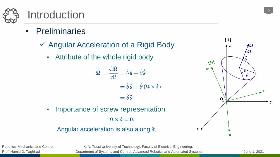
• Preliminaries
Angular Acceleration of a Rigid Body
Attribute of the whole rigid body
Importance of screw representation
𝛀 × ො𝒔 = 𝟎.
Angular acceleration is also along ො𝒔.
5
(𝛀 × ො𝒔)
Robotics: Mechanics and Control K. N. Toosi University of Technology, Faculty of Electrical Engineering,
Prof. Hamid D. Taghirad Department of Systems and Control, Advanced Robotics and Automated Systems June 1, 2021
Preliminaries
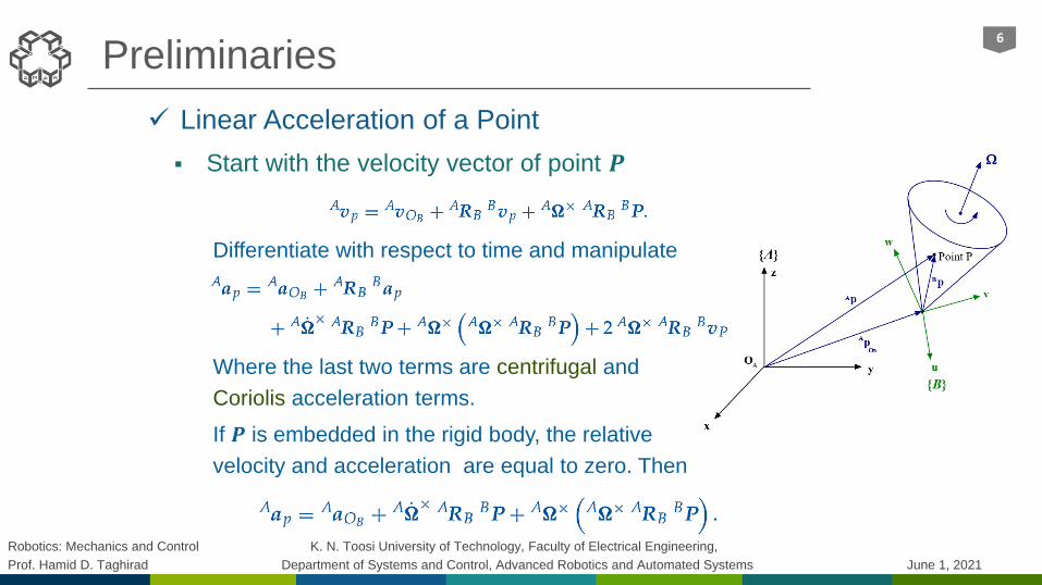
Linear Acceleration of a Point
Start with the velocity vector of point 𝑷
Differentiate with respect to time and manipulate
Where the last two terms are centrifugal and
Coriolis acceleration terms.
If 𝑷 is embedded in the rigid body, the relative
velocity and acceleration are equal to zero. Then
6
Robotics: Mechanics and Control K. N. Toosi University of Technology, Faculty of Electrical Engineering,
Prof. Hamid D. Taghirad Department of Systems and Control, Advanced Robotics and Automated Systems June 1, 2021
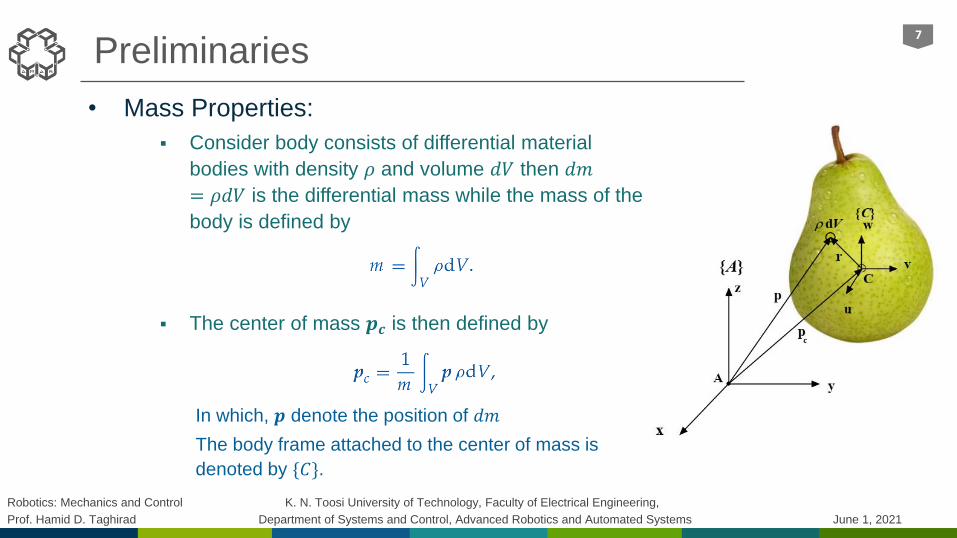
Preliminaries
• Mass Properties:
Consider body consists of differential material
bodies with density 𝜌 and volume 𝑑𝑉 then 𝑑𝑚
= 𝜌𝑑𝑉 is the differential mass while the mass of the
body is defined by
The center of mass 𝒑𝒄 is then defined by
In which, 𝒑 denote the position of 𝑑𝑚
The body frame attached to the center of mass is
denoted by {𝐶}.
7
Robotics: Mechanics and Control K. N. Toosi University of Technology, Faculty of Electrical Engineering,
Prof. Hamid D. Taghirad Department of Systems and Control, Advanced Robotics and Automated Systems June 1, 2021
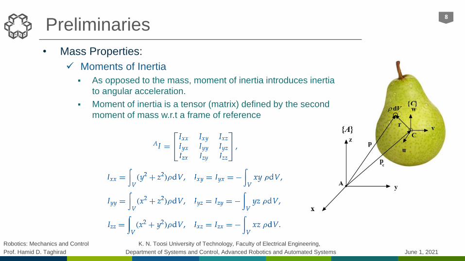
Preliminaries
• Mass Properties:
Moments of Inertia
As opposed to the mass, moment of inertia introduces inertia
to angular acceleration.
Moment of inertia is a tensor (matrix) defined by the second
moment of mass w.r.t a frame of reference
8
Robotics: Mechanics and Control K. N. Toosi University of Technology, Faculty of Electrical Engineering,
Prof. Hamid D. Taghirad Department of Systems and Control, Advanced Robotics and Automated Systems June 1, 2021
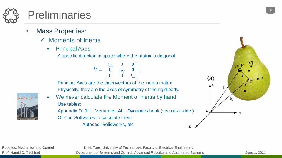
Preliminaries
• Mass Properties:
Moments of Inertia
Principal Axes:
A specific direction in space where the matrix is diagonal
Principal Axes are the eigenvectors of the inertia matrix
Physically, they are the axes of symmetry of the rigid body.
We never calculate the Moment of inertia by hand
Use tables:
Appendix D: J. L. Meriam et. Al. : Dynamics book (see next slide )
Or Cad Softwares to calculate them.
Autocad, Solidworks, etc
9

Robotics: Mechanics and Control K. N. Toosi University of Technology, Faculty of Electrical Engineering,
Prof. Hamid D. Taghirad Department of Systems and Control, Advanced Robotics and Automated Systems June 1, 2021
Preliminaries
• Mass Properties:
Moments of Inertia Table:
10
Robotics: Mechanics and Control K. N. Toosi University of Technology, Faculty of Electrical Engineering,
Prof. Hamid D. Taghirad Department of Systems and Control, Advanced Robotics and Automated Systems June 1, 2021
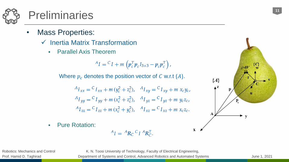
Preliminaries
• Mass Properties:
Inertia Matrix Transformation
Parallel Axis Theorem
Where 𝑝𝑐 denotes the position vector of 𝐶 w.r.t {𝐴}.
Pure Rotation:
11
Robotics: Mechanics and Control K. N. Toosi University of Technology, Faculty of Electrical Engineering,
Prof. Hamid D. Taghirad Department of Systems and Control, Advanced Robotics and Automated Systems June 1, 2021
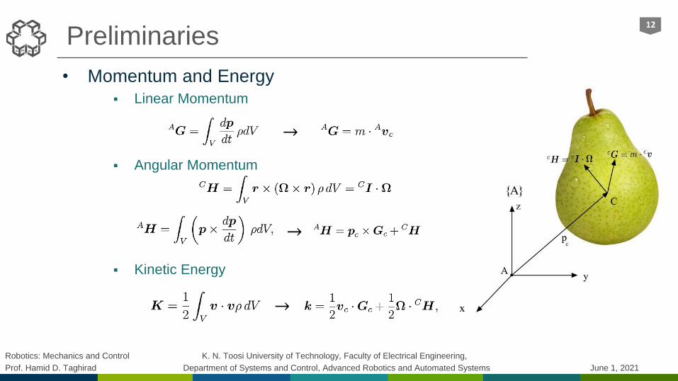
Preliminaries
• Momentum and Energy
Linear Momentum
Angular Momentum
Kinetic Energy
12
→
→
→

Robotics: Mechanics and Control K. N. Toosi University of Technology, Faculty of Electrical Engineering,
Prof. Hamid D. Taghirad Department of Systems and Control, Advanced Robotics and Automated Systems June 1, 2021
Contents
In this chapter we review the dynamics analysis for serial robots. First the definition to angular and linear accelerations are given, then mass properties, linear and angular momentums, and kinetic energy of a rigid body in space is defined. Lagrange formulation is given in general form, and dynamics mass matrix, gravity and Coriolis and centrifugal vectors are defined and derived for several case studies. Dynamic formulation properties is given next, then actuator dynamics is elaborated for electrically driven robots with gearbox. Finally, linear regression method is used for dynamics calibration, and model verification methods are elaborated by introducing consistency measure.
13
Actuator DynamicsElectrical actuators, permanent magnet DC motors, servo amplifiers, gearbox, motor-gearbox-load dynamics, motor-gearbox-multiple joint robot,
4
Dynamics CalibrationLinear Regression, linear model with constant gravity, house holder reflection, varying gravity term, filtered velocity, model verification, consistency measure.
5
PreliminariesAngular acceleration, linear acceleration of a point, mass properties, center of mass, moments of inertia, inertia matrix transformations, linear and angular momentum, kinetic energy.
1
Lagrange FormulationMotivating example, generalized coordinates and forces, kinetic energy, mass matrix, potential energy, gravity vector, Coriolis and centrifugal vector, case studies.
2
Dynamic Formulation PropertiesMass matrix properties, linearity in parameters, Christoffel Matrix, skew-symmetric property, general dynamic formulation, passivity,
3
Robotics: Mechanics and Control K. N. Toosi University of Technology, Faculty of Electrical Engineering,
Prof. Hamid D. Taghirad Department of Systems and Control, Advanced Robotics and Automated Systems June 1, 2021
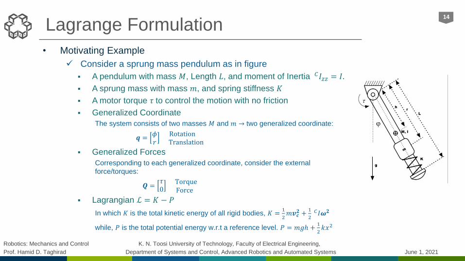
Lagrange Formulation
• Motivating Example
Consider a sprung mass pendulum as in figure
A pendulum with mass 𝑀, Length 𝐿, and moment of Inertia 𝐶𝐼𝑧𝑧 = 𝐼.
A sprung mass with mass 𝑚, and spring stiffness 𝐾
A motor torque 𝜏 to control the motion with no friction
Generalized Coordinate
The system consists of two masses 𝑀 and 𝑚 → two generalized coordinate:
𝒒 =𝜙𝑟
RotationTranslation
Generalized Forces
Corresponding to each generalized coordinate, consider the external
force/torques:
𝑸 =𝜏0
TorqueForce
Lagrangian ℒ = 𝐾 − 𝑃
In which 𝐾 is the total kinetic energy of all rigid bodies, 𝐾 =1
2𝑚𝒗𝒄
𝟐 +1
2𝐶𝐼𝝎𝟐
while, 𝑃 is the total potential energy w.r.t a reference level. 𝑃 = 𝑚𝑔ℎ +1
2𝑘𝑥2
14
Robotics: Mechanics and Control K. N. Toosi University of Technology, Faculty of Electrical Engineering,
Prof. Hamid D. Taghirad Department of Systems and Control, Advanced Robotics and Automated Systems June 1, 2021
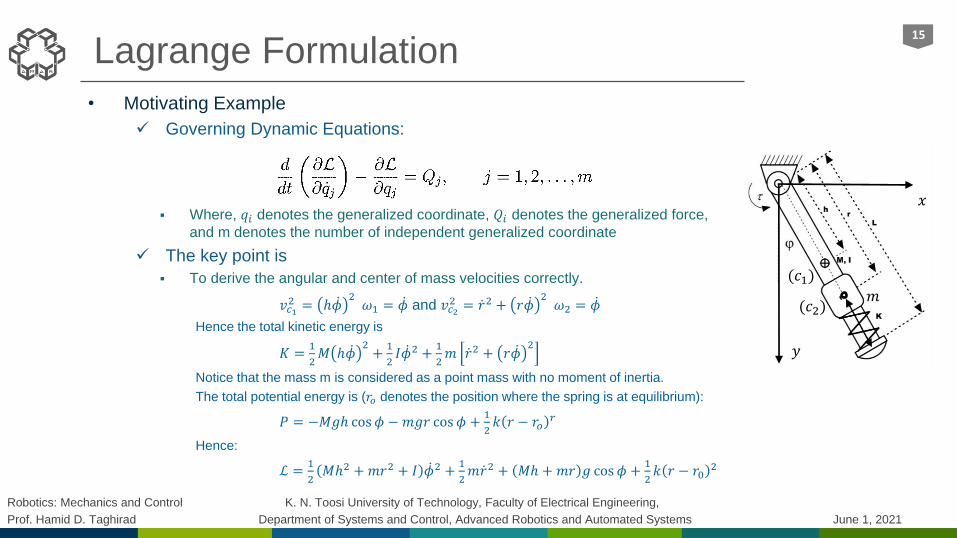
Lagrange Formulation
• Motivating Example
Governing Dynamic Equations:
Where, 𝑞𝑖 denotes the generalized coordinate, 𝑄𝑖 denotes the generalized force,
and m denotes the number of independent generalized coordinate
The key point is
To derive the angular and center of mass velocities correctly.
𝑣𝑐12 = ℎ ሶ𝜙
2𝜔1 = ሶ𝜙 and 𝑣𝑐2
2 = ሶ𝑟2 + 𝑟 ሶ𝜙2𝜔2 = ሶ𝜙
Hence the total kinetic energy is
𝐾 =1
2𝑀 ℎ ሶ𝜙
2+
1
2𝐼 ሶ𝜙2 +
1
2𝑚 ሶ𝑟2 + 𝑟 ሶ𝜙
2
Notice that the mass m is considered as a point mass with no moment of inertia.
The total potential energy is (𝑟𝑜 denotes the position where the spring is at equilibrium):
𝑃 = −𝑀𝑔ℎ cos𝜙 − 𝑚𝑔𝑟 cos 𝜙 +1
2𝑘 𝑟 − 𝑟𝑜
𝑟
Hence:
ℒ =1
2𝑀ℎ2 +𝑚𝑟2 + 𝐼 ሶ𝜙2 +
1
2𝑚 ሶ𝑟2 + 𝑀ℎ +𝑚𝑟 𝑔 cos 𝜙 +
1
2𝑘 𝑟 − 𝑟0
2
𝑚
𝑦
𝑥
(𝑐1)
(𝑐2)
15
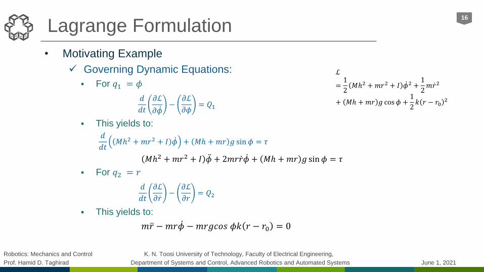
Robotics: Mechanics and Control K. N. Toosi University of Technology, Faculty of Electrical Engineering,
Prof. Hamid D. Taghirad Department of Systems and Control, Advanced Robotics and Automated Systems June 1, 2021
Lagrange Formulation
• Motivating Example
Governing Dynamic Equations:
For 𝑞1 = 𝜙
𝑑
𝑑𝑡
𝜕ℒ
𝜕 ሶ𝜙−
𝜕ℒ
𝜕𝜙= 𝑄1
This yields to:
𝑑
𝑑𝑡𝑀ℎ2 +𝑚𝑟2 + 𝐼 ሶ𝜙 + 𝑀ℎ +𝑚𝑟 𝑔 sin𝜙 = 𝜏
𝑀ℎ2 +𝑚𝑟2 + 𝐼 ሷ𝜙 + 2𝑚𝑟 ሶ𝑟 ሶ𝜙 + 𝑀ℎ +𝑚𝑟 𝑔 sin𝜙 = 𝜏
For 𝑞2 = 𝑟
𝑑
𝑑𝑡
𝜕ℒ
𝜕 ሶ𝑟−
𝜕ℒ
𝜕𝑟= 𝑄2
This yields to:
𝑚 ሷ𝑟 − 𝑚𝑟 ሶ𝜙 − 𝑚𝑟𝑔𝑐𝑜𝑠 𝜙𝑘 𝑟 − 𝑟0 = 0
16
ℒ
=1
2𝑀ℎ2 +𝑚𝑟2 + 𝐼 ሶ𝜙2 +
1
2𝑚 ሶ𝑟2
+ 𝑀ℎ +𝑚𝑟 𝑔 cos 𝜙 +1
2𝑘 𝑟 − 𝑟0
2
Robotics: Mechanics and Control K. N. Toosi University of Technology, Faculty of Electrical Engineering,
Prof. Hamid D. Taghirad Department of Systems and Control, Advanced Robotics and Automated Systems June 1, 2021
Lagrange Formulation
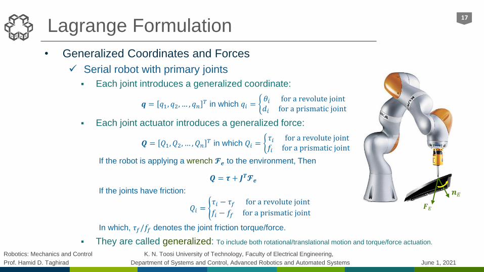
• Generalized Coordinates and Forces
Serial robot with primary joints
Each joint introduces a generalized coordinate:
𝒒 = 𝑞1, 𝑞2, … , 𝑞𝑛𝑇 in which 𝑞𝑖 = ቊ
𝜃𝑖 for a revolute joint𝑑𝑖 for a prismatic joint
Each joint actuator introduces a generalized force:
𝑸 = 𝑄1, 𝑄2, … , 𝑄𝑛𝑇 in which 𝑄𝑖 = ቊ
𝜏𝑖 for a revolute joint𝑓𝑖 for a prismatic joint
If the robot is applying a wrench 𝓕𝒆 to the environment, Then
𝑸 = 𝝉 + 𝑱𝑻𝓕𝒆
If the joints have friction:
𝑄𝑖 = ൝𝜏𝑖 − 𝜏𝑓 for a revolute joint
𝑓𝑖 − 𝑓𝑓 for a prismatic joint
In which, 𝜏𝑓/𝑓𝑓 denotes the joint friction torque/force.
They are called generalized: To include both rotational/translational motion and torque/force actuation.
17
𝑭𝐸
𝒏𝐸
Robotics: Mechanics and Control K. N. Toosi University of Technology, Faculty of Electrical Engineering,
Prof. Hamid D. Taghirad Department of Systems and Control, Advanced Robotics and Automated Systems June 1, 2021
Lagrange Formulation
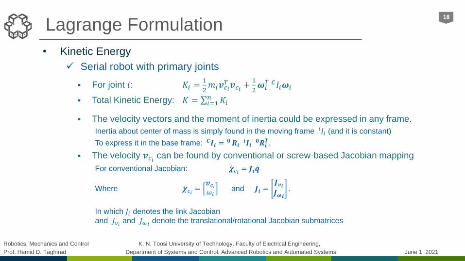
• Kinetic Energy
Serial robot with primary joints
For joint 𝑖: 𝐾𝑖 =1
2𝑚𝑖𝒗𝑐𝑖
𝑇 𝒗𝑐𝑖 +1
2𝝎𝑖𝑇 𝐶𝐼𝑖𝝎𝑖
Total Kinetic Energy: 𝐾 = σ𝑖=1𝑛 𝐾𝑖
The velocity vectors and the moment of inertia could be expressed in any frame.
Inertia about center of mass is simply found in the moving frame 𝑖𝐼𝑖 (and it is constant)
To express it in the base frame: 𝑪𝑰𝒊 =𝟎𝑹𝒊
𝒊𝑰𝒊𝟎𝑹𝒊
𝑻.
The velocity 𝒗𝑐𝑖 can be found by conventional or screw-based Jacobian mapping
For conventional Jacobian: ሶ𝝌𝑐𝑖 = 𝑱𝒊 ሶ𝒒
Where ሶ𝝌𝑐𝑖 =𝒗𝑐𝑖𝜔𝑖
and 𝑱𝒊 =𝑱𝒗𝒊𝑱𝝎𝒊
.
In which 𝐽𝑖 denotes the link Jacobian
and 𝐽𝑣𝑖 and 𝐽𝜔𝑖 denote the translational/rotational Jacobian submatrices
18
Robotics: Mechanics and Control K. N. Toosi University of Technology, Faculty of Electrical Engineering,
Prof. Hamid D. Taghirad Department of Systems and Control, Advanced Robotics and Automated Systems June 1, 2021
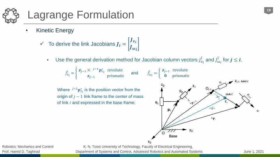
Lagrange Formulation
• Kinetic Energy
To derive the link Jacobians 𝑱𝒊 =𝑱𝒗𝒊𝑱𝝎𝒊
Use the general derivation method for Jacobian column vectors 𝐽𝑣𝑖j
and 𝐽𝜔𝑖
jfor 𝒋 ≤ 𝒊.
𝐽𝑣𝑖j= ൝
𝒛𝑗−1 ×𝑗−1𝒑𝑐𝑖
∗ revolute
𝒛𝑗−1 prismaticand 𝐽𝜔𝑖
j= ቊ
𝒛𝑗−1 revolute
𝟎 prismatic
Where 𝑗−1𝒑𝑐𝑖∗ is the position vector from the
origin of 𝑗 − 1 link frame to the center of mass
of link 𝑖 and expressed in the base frame.
19
Robotics: Mechanics and Control K. N. Toosi University of Technology, Faculty of Electrical Engineering,
Prof. Hamid D. Taghirad Department of Systems and Control, Advanced Robotics and Automated Systems June 1, 2021
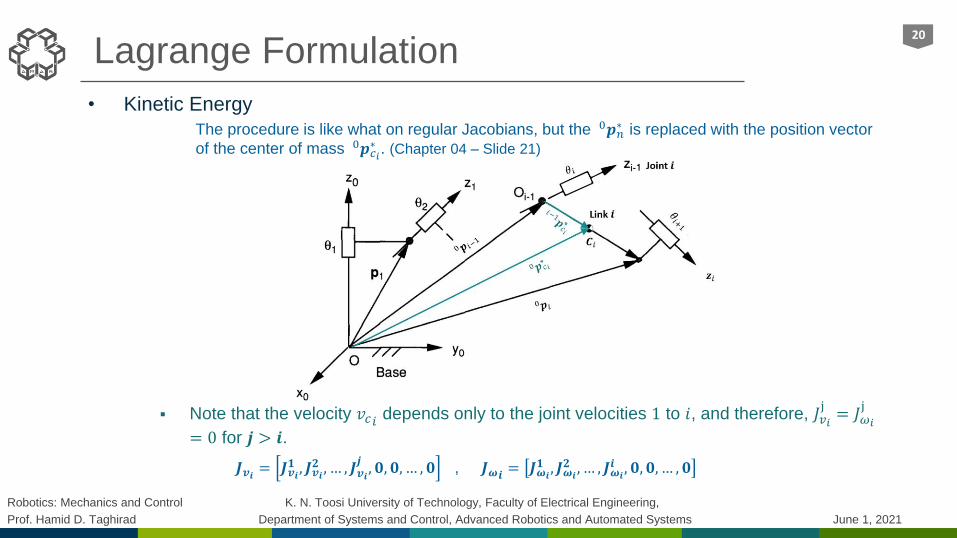
• Kinetic Energy
The procedure is like what on regular Jacobians, but the 0𝒑𝑛∗ is replaced with the position vector
of the center of mass 0𝒑𝑐𝑖∗ . (Chapter 04 – Slide 21)
Note that the velocity 𝑣𝑐𝑖 depends only to the joint velocities 1 to 𝑖, and therefore, 𝐽𝑣𝑖j= 𝐽𝜔𝑖
j
= 0 for 𝒋 > 𝒊.
𝑱𝒗𝒊 = 𝑱𝒗𝒊𝟏 , 𝑱𝒗𝒊
𝟐 , … , 𝑱𝒗𝒊𝒋, 𝟎, 𝟎, … , 𝟎 , 𝑱𝝎𝒊 = 𝑱𝝎𝒊
𝟏 , 𝑱𝝎𝒊𝟐 , … , 𝑱𝝎𝒊
𝒊 , 𝟎, 𝟎, … , 𝟎
Lagrange Formulation20
Robotics: Mechanics and Control K. N. Toosi University of Technology, Faculty of Electrical Engineering,
Prof. Hamid D. Taghirad Department of Systems and Control, Advanced Robotics and Automated Systems June 1, 2021
Lagrange Formulation
• Kinetic Energy Therefore, 𝐾 =
1
2σ𝑖=1𝑛 (𝑚𝑖𝒗𝑐𝑖
𝑇 𝒗𝑐𝑖 +𝝎𝑖𝑇 𝐶𝐼𝑖𝝎𝑖)
Use Jacobians: =1
2ሶ𝒒𝑇 σ𝑖=1
𝑛 (𝑚𝑖 𝑱𝒗𝒊𝑻 𝑱𝒗𝒊+ 𝑱𝝎
𝑻𝒊
𝐶𝐼𝑖 𝑱𝝎𝒊) ሶ𝒒
Define Mass Matrix:
By this means: 𝐾 =1
2ሶ𝒒𝑇𝑴 𝒒 ሶ𝒒
The Mass Matrix is a symmetric, and positive definite matrix.
The kinetic energy is also always positive unless the system is at rest.
• Potential Energy
The work required to displace link 𝑖 to position 𝒑𝑐𝑖 is given by −𝑚𝑖𝒈𝑇𝒑𝑐𝑖, in which 𝒈 is the vector of gravity
acceleration, Therefore,
𝑃 = −σ𝑖=1𝑛 𝑚𝑖𝒈
𝑇 𝟎𝒑𝑐𝑖
If there is any spring (flexibility) in joints, then
In which 𝑘𝑖 denote the spring stiffness while Δ𝑥 denote its deflection
21
𝑴(𝒒) =
𝑖=1
𝑛
(𝑚𝑖 𝑱𝒗𝒊𝑻 𝑱𝒗𝒊+ 𝑱𝝎
𝑻𝒊
𝐶𝐼𝑖 𝑱𝝎𝒊)
𝑃 = −
𝑖=1
𝑛
𝑚𝑖𝒈𝑇 𝟎𝒑𝑐𝑖 +
1
2
𝑖=1
𝑛
𝑘𝑖 Δ𝑥2
Robotics: Mechanics and Control K. N. Toosi University of Technology, Faculty of Electrical Engineering,
Prof. Hamid D. Taghirad Department of Systems and Control, Advanced Robotics and Automated Systems June 1, 2021
Lagrange Formulation
• General Formulation
Consider 𝑛DoF serial manipulator with primary joints
Denote 𝒒 = 𝑞1, 𝑞2, … , 𝑞𝑛𝑻 as the generalized coordinates and
Denote 𝑸 = 𝑄1, 𝑄2, … , 𝑄𝑛𝑻 as the generalized Forces.
Form Lagrangian by ℒ = 𝐾 − 𝑃
Derive the governing equation of motion in vector form by:
𝑑
𝑑𝑡
𝜕ℒ
𝜕 ሶ𝒒−𝜕ℒ
𝜕𝒒= 𝑸
in which, ℒ = 𝐾(𝒒, ሶ𝒒) − 𝑃(𝒒)
hence, 𝑑
𝑑𝑡
𝜕ℒ
𝜕 ሶ𝒒=
𝑑
𝑑𝑡
𝜕𝐾
𝜕 ሶ𝒒=
𝑑
𝑑𝑡𝑀 𝑞 ሶ𝒒 = 𝑴 𝒒 ሷ𝒒 + ሶ𝑴 𝒒 ሶ𝒒
Furthermore, define the gravity vector as g 𝒒 =𝜕𝑃
𝜕𝒒= −σ𝑖=1
𝑛 𝜕𝑃
𝜕𝒒𝑚𝑖𝒈
𝑇 𝟎𝒑𝑐𝑖 = −σ𝑖=1𝑛 𝑚𝑖𝑱𝒗𝒊
𝑻 𝒈.
In which, 𝑱𝒗𝒊𝑻 denotes the linear velocity Jacobian of each center of motion. Hence the dynamics is written as:
𝑴 𝒒 ሷ𝒒 + ሶ𝑴 𝒒 ሶ𝒒 −𝜕𝐾
𝜕𝒒+ g 𝒒 = 𝑸
22
Robotics: Mechanics and Control K. N. Toosi University of Technology, Faculty of Electrical Engineering,
Prof. Hamid D. Taghirad Department of Systems and Control, Advanced Robotics and Automated Systems June 1, 2021
Lagrange Formulation
• General Formulation
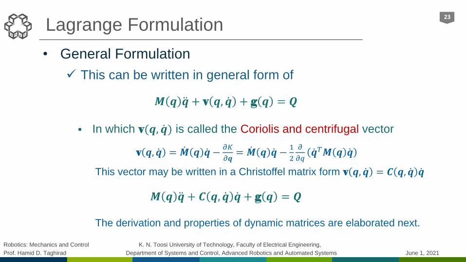
This can be written in general form of
𝑴 𝒒 ሷ𝒒 + v 𝒒, ሶ𝒒 + g 𝒒 = 𝑸
In which v(𝒒, ሶ𝒒) is called the Coriolis and centrifugal vector
v 𝒒, ሶ𝒒 = ሶ𝑴 𝒒 ሶ𝒒 −𝜕𝐾
𝜕𝒒= ሶ𝑴 𝒒 ሶ𝒒 −
1
2
𝜕
𝜕𝑞ሶ𝒒𝑇𝑴 𝒒 ሶ𝒒
This vector may be written in a Christoffel matrix form v 𝒒, ሶ𝒒 = 𝑪 𝒒, ሶ𝒒 ሶ𝒒
𝑴 𝒒 ሷ𝒒 + 𝑪 𝒒, ሶ𝒒 ሶ𝒒 + g 𝒒 = 𝑸
The derivation and properties of dynamic matrices are elaborated next.
23
Robotics: Mechanics and Control K. N. Toosi University of Technology, Faculty of Electrical Engineering,
Prof. Hamid D. Taghirad Department of Systems and Control, Advanced Robotics and Automated Systems June 1, 2021
𝑥
𝑦
𝜃1
𝜃2
Lagrange Formulation
• Examples:
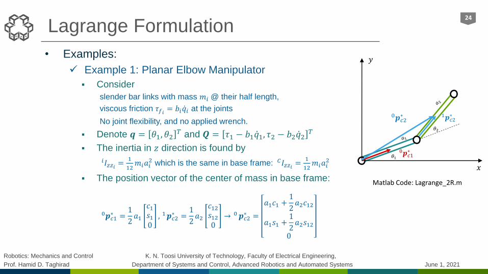
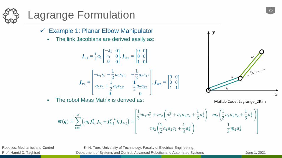
Example 1: Planar Elbow Manipulator
Consider
slender bar links with mass 𝑚𝑖 @ their half length,
viscous friction 𝜏𝑓𝑖 = 𝑏𝑖 ሶ𝑞𝑖 at the joints
No joint flexibility, and no applied wrench.
Denote 𝒒 = 𝜃1, 𝜃2𝑇 and 𝑸 = 𝜏1 − 𝑏1 ሶ𝑞1, 𝜏2 − 𝑏2 ሶ𝑞2
𝑇
The inertia in 𝑧 direction is found by
𝑖𝐼𝑧𝑧𝑖 =1
12𝑚𝑖𝑎𝑖
2 which is the same in base frame: 𝐶𝐼𝑧𝑧𝑖 =1
12𝑚𝑖𝑎𝑖
2
The position vector of the center of mass in base frame:
0𝒑𝑐1∗ =
1
2𝑎1
𝑐1𝑠10
, 1𝒑𝑐2∗ =
1
2𝑎2
𝑐12𝑠120
→ 0𝒑𝑐2∗ =
𝑎1𝑐1 +1
2𝑎2𝑐12
𝑎1𝑠1 +1
2𝑎2𝑠12
0
24
0𝒑𝑐1∗
0𝒑𝑐2∗ 1𝒑𝑐2
∗
Matlab Code: Lagrange_2R.m
Robotics: Mechanics and Control K. N. Toosi University of Technology, Faculty of Electrical Engineering,
Prof. Hamid D. Taghirad Department of Systems and Control, Advanced Robotics and Automated Systems June 1, 2021
Lagrange Formulation
Example 1: Planar Elbow Manipulator
The link Jacobians are derived easily as:
𝑱𝒗𝟏 =1
2𝑎1
−𝑠1𝑐10
000
, 𝑱𝝎𝟏=
001
000
𝑱𝒗𝟐 =
−𝑎1𝑠1 −1
2𝑎2𝑠12
𝑎1𝑐1 +1
2𝑎2𝑐12
0
−1
2𝑎2𝑠12
1
2𝑎2𝑐12
0
, 𝑱𝝎𝟐=
001
001
The robot Mass Matrix is derived as:
𝑴 𝒒 =
𝑖=1
2
𝑚𝑖 𝑱𝒗𝒊𝑻 𝑱𝒗𝒊+ 𝑱𝝎
𝑻𝒊
𝐶𝐼𝑖 𝑱𝝎𝒊 =
1
3𝑚1𝑎1
2 +𝑚2 𝑎12 + 𝑎1𝑎2𝑐2 +
1
3𝑎22 𝑚2
1
2𝑎1𝑎2𝑐2 +
1
3𝑎22
𝑚2
1
2𝑎1𝑎2𝑐2 +
1
3𝑎22
1
3𝑚2𝑎2
2
25
𝑥
𝑦
𝜃1
𝜃2
Matlab Code: Lagrange_2R.m
Robotics: Mechanics and Control K. N. Toosi University of Technology, Faculty of Electrical Engineering,
Prof. Hamid D. Taghirad Department of Systems and Control, Advanced Robotics and Automated Systems June 1, 2021
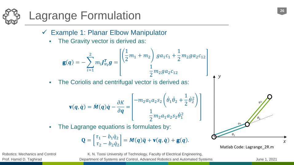
Lagrange Formulation
Example 1: Planar Elbow Manipulator
The Gravity vector is derived as:
g 𝒒 = −
𝑖=1
2
𝑚𝑖𝑱𝒗𝒊𝑻 𝒈 =
1
2𝑚1 +𝑚2 𝑔𝑎1𝑐1 +
1
2𝑚2𝑔𝑎2𝑐12
1
2𝑚2𝑔𝑎2𝑐12
The Coriolis and centrifugal vector is derived as:
v 𝒒, ሶ𝒒 = ሶ𝑴 𝒒 ሶ𝒒 −𝜕𝐾
𝜕𝒒=
−𝑚2𝑎1𝑎2𝑠2 ሶ𝜃1 ሶ𝜃2 +1
2ሶ𝜃22
1
2𝑚2𝑎1𝑎2𝑠2 ሶ𝜃1
2
The Lagrange equations is formulates by:
𝐐 =𝜏1 − 𝑏1 ሶ𝑞2𝜏2 − 𝑏2 ሶ𝑞2
= 𝑴 𝒒 ሷ𝒒 + v 𝒒, ሶ𝒒 + g 𝒒 .
26
𝑥
𝑦
𝜃1
𝜃2
Matlab Code: Lagrange_2R.m
Robotics: Mechanics and Control K. N. Toosi University of Technology, Faculty of Electrical Engineering,
Prof. Hamid D. Taghirad Department of Systems and Control, Advanced Robotics and Automated Systems June 1, 2021
Lagrange Formulation
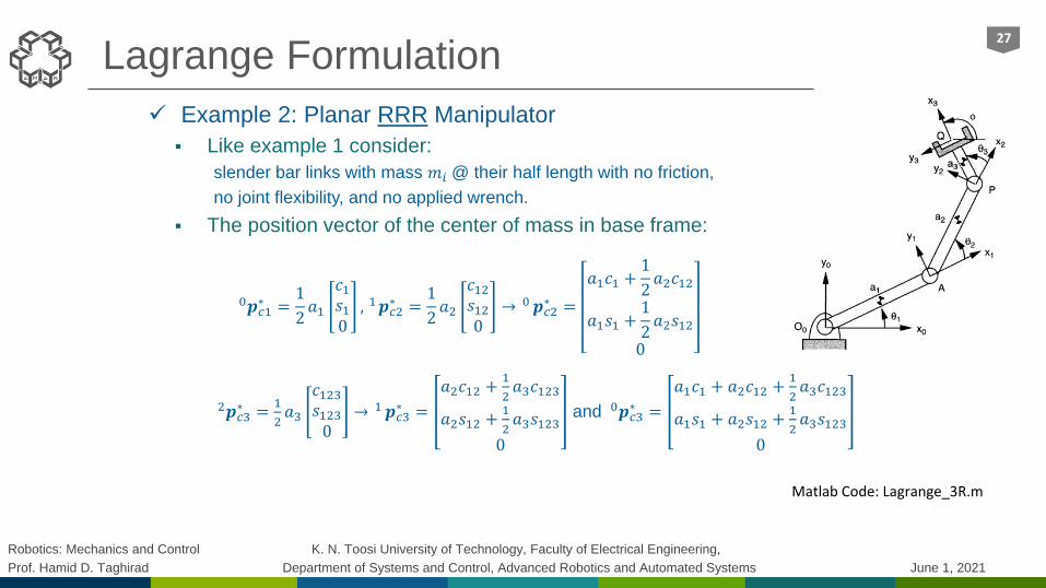
Example 2: Planar RRR Manipulator
Like example 1 consider:
slender bar links with mass 𝑚𝑖 @ their half length with no friction,
no joint flexibility, and no applied wrench.
The position vector of the center of mass in base frame:
0𝒑𝑐1∗ =
1
2𝑎1
𝑐1𝑠10
, 1𝒑𝑐2∗ =
1
2𝑎2
𝑐12𝑠120
→ 0𝒑𝑐2∗ =
𝑎1𝑐1 +1
2𝑎2𝑐12
𝑎1𝑠1 +1
2𝑎2𝑠12
0
2𝒑𝑐3∗ =
1
2𝑎3
𝑐123𝑠1230
→ 1𝒑𝑐3∗ =
𝑎2𝑐12 +1
2𝑎3𝑐123
𝑎2𝑠12 +1
2𝑎3𝑠123
0
and 0𝒑𝑐3∗ =
𝑎1𝑐1 + 𝑎2𝑐12 +1
2𝑎3𝑐123
𝑎1𝑠1 + 𝑎2𝑠12 +1
2𝑎3𝑠123
0
27
Matlab Code: Lagrange_3R.m

Robotics: Mechanics and Control K. N. Toosi University of Technology, Faculty of Electrical Engineering,
Prof. Hamid D. Taghirad Department of Systems and Control, Advanced Robotics and Automated Systems June 1, 2021
Lagrange Formulation
Example 2: Planar RRR Manipulator
The link Jacobians are derived easily as:
𝑱𝒗𝟏 =1
2𝑎1
−𝑠1𝑐10
000
000
, 𝑱𝝎𝟏=
001
000
000
𝑱𝒗𝟐 =
−𝑎1𝑠1 −1
2𝑎2𝑠12 −
1
2𝑎2𝑠12 0
𝑎1𝑐1 +1
2𝑎2𝑐12
1
2𝑎2𝑐12 0
0 0 0
, 𝑱𝝎𝟐=
001
001
000
𝑱𝒗𝟑 =
−𝑎1𝑠1 − 𝑎2𝑠12 −1
2𝑎3𝑠123
𝑎1𝑐1 + 𝑎2𝑐12 +1
2𝑎3𝑐𝑠123
0
−𝑎2𝑠12 −1
2𝑎3𝑠123
𝑎2𝑐12 +1
2𝑎3𝑐123
0
−1
2𝑎3𝑠123
1
2𝑎3𝑐123
0
, 𝑱𝝎𝟑=
001
001
001
28
Matlab Code: Lagrange_3R.m
Robotics: Mechanics and Control K. N. Toosi University of Technology, Faculty of Electrical Engineering,
Prof. Hamid D. Taghirad Department of Systems and Control, Advanced Robotics and Automated Systems June 1, 2021
Lagrange Formulation
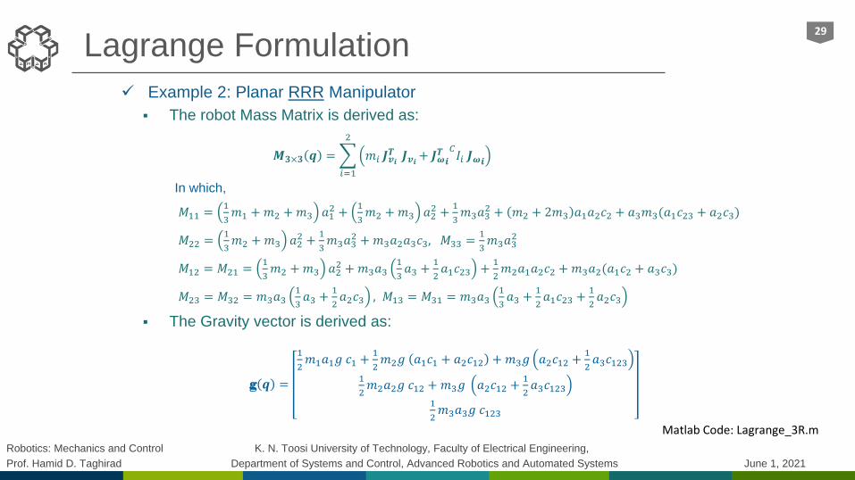
Example 2: Planar RRR Manipulator
The robot Mass Matrix is derived as:
𝑴𝟑×𝟑 𝒒 =
𝑖=1
2
𝑚𝑖 𝑱𝒗𝒊𝑻 𝑱𝒗𝒊+ 𝑱𝝎
𝑻𝒊
𝐶𝐼𝑖 𝑱𝝎𝒊
In which,
𝑀11 =1
3𝑚1 +𝑚2 +𝑚3 𝑎1
2 +1
3𝑚2 +𝑚3 𝑎2
2 +1
3𝑚3𝑎3
2 + 𝑚2 + 2𝑚3 𝑎1𝑎2𝑐2 + 𝑎3𝑚3(𝑎1𝑐23 + 𝑎2𝑐3)
𝑀22 =1
3𝑚2 +𝑚3 𝑎2
2 +1
3𝑚3𝑎3
2 +𝑚3𝑎2𝑎3𝑐3, 𝑀33 =1
3𝑚3𝑎3
2
𝑀12 = 𝑀21 =1
3𝑚2 +𝑚3 𝑎2
2 +𝑚3𝑎31
3𝑎3 +
1
2𝑎1𝑐23 +
1
2𝑚2𝑎1𝑎2𝑐2 +𝑚3𝑎2(𝑎1𝑐2 + 𝑎3𝑐3)
𝑀23 = 𝑀32 = 𝑚3𝑎31
3𝑎3 +
1
2𝑎2𝑐3 , 𝑀13 = 𝑀31 = 𝑚3𝑎3
1
3𝑎3 +
1
2𝑎1𝑐23 +
1
2𝑎2𝑐3
The Gravity vector is derived as:
g 𝒒 =
1
2𝑚1𝑎1𝑔 𝑐1 +
1
2𝑚2𝑔 𝑎1𝑐1 + 𝑎2𝑐12 +𝑚3𝑔 𝑎2𝑐12 +
1
2𝑎3𝑐123
1
2𝑚2𝑎2𝑔 𝑐12 +𝑚3𝑔 𝑎2𝑐12 +
1
2𝑎3𝑐123
1
2𝑚3𝑎3𝑔 𝑐123
29
Matlab Code: Lagrange_3R.m
Robotics: Mechanics and Control K. N. Toosi University of Technology, Faculty of Electrical Engineering,
Prof. Hamid D. Taghirad Department of Systems and Control, Advanced Robotics and Automated Systems June 1, 2021
Lagrange Formulation
Example 2: Planar RRR Manipulator
The Coriolis and centrifugal vector is derived as:
𝑽 𝒒, ሶ𝒒 = ሶ𝑴 𝒒 ሶ𝒒 −1
2
𝜕
𝜕𝑞ሶ𝒒𝑇𝑴 𝒒 ሶ𝒒 =
𝑉1𝑉2𝑉3
In which,
𝑉1 = − ሶ𝜃1 ሶ𝜃2 𝑎1𝑎3𝑚3𝑠23 + 𝑎1𝑎2𝑚2𝑠2 + 2𝑎1𝑎2𝑚3𝑠2 + ሶ𝜃3 𝑎1𝑎3𝑚3𝑠23 + 𝑎2𝑎3𝑚3𝑠3
− ሶ𝜃2 ሶ𝜃21
2𝑎1𝑎3𝑚3𝑠23 +
1
2𝑎1𝑎2𝑚2𝑠2 + 𝑎1𝑎2𝑚3𝑠2 + ሶ𝜃3
1
2𝑎1𝑎3𝑚3𝑠23 + 𝑎2𝑎3𝑚3𝑠3
− ሶ𝜃3 𝑎3𝑚3ሶ𝜃3
1
2𝑎1𝑠23 +
1
2𝑎2𝑠3 +
1
2𝑎1𝑎3𝑚3𝑠23 ሶ𝜃2
𝑉2 =1
2𝑎1𝑎3𝑚3𝑠23 + 𝑎1𝑎2𝑚2𝑠2 + 𝑎1𝑎2𝑚3𝑠2 ሶ𝜃1
2 −1
2𝑎2𝑎3𝑚3𝑠3 ሶ𝜃3
2 − 𝑎2𝑎3𝑚3𝑠3 ሶ𝜃1 ሶ𝜃3 + ሶ𝜃2 ሶ𝜃3
𝑉3 =1
2𝑚3𝑎3((𝑎1𝑠23 + 𝑎2𝑠3) ሶ𝜃1
2 + 𝑎2𝑠3 ሶ𝜃22 + 2𝑎2𝑠3 ሶ𝜃1 ሶ𝜃2
The Lagrange equations is formulates by:
𝐐 =
𝜏1𝜏2𝜏3
= 𝑴 𝒒 ሷ𝒒 + 𝑽 𝒒, ሶ𝒒 + 𝑮 𝒒 .
30
Matlab Code: Lagrange_3R.m
Robotics: Mechanics and Control K. N. Toosi University of Technology, Faculty of Electrical Engineering,
Prof. Hamid D. Taghirad Department of Systems and Control, Advanced Robotics and Automated Systems June 1, 2021
Lagrange Formulation
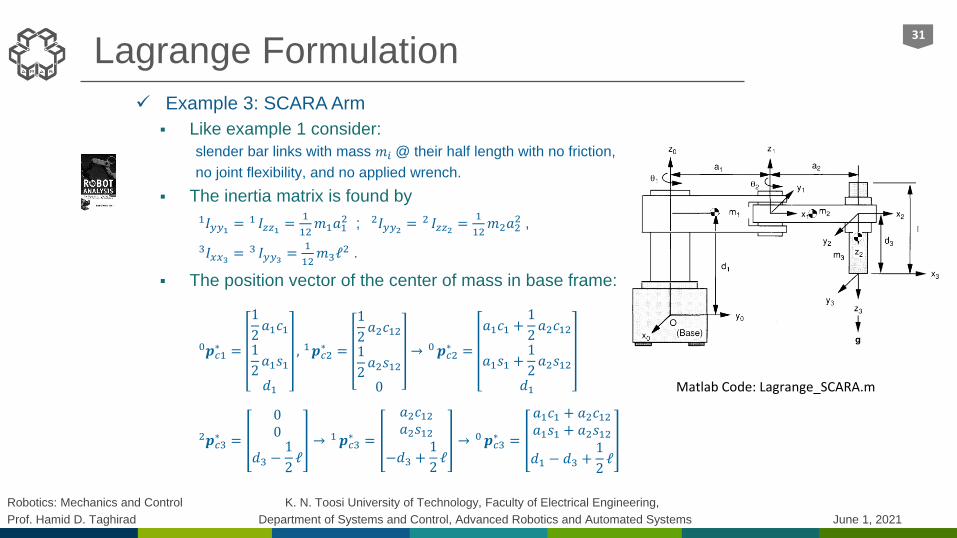
Example 3: SCARA Arm
Like example 1 consider:
slender bar links with mass 𝑚𝑖 @ their half length with no friction,
no joint flexibility, and no applied wrench.
The inertia matrix is found by
1𝐼𝑦𝑦1 =1 𝐼𝑧𝑧1 =
1
12𝑚1𝑎1
2 ; 2𝐼𝑦𝑦2 =2 𝐼𝑧𝑧2 =
1
12𝑚2𝑎2
2 ,
3𝐼𝑥𝑥3 =3 𝐼𝑦𝑦3 =
1
12𝑚3ℓ
2 .
The position vector of the center of mass in base frame:
0𝒑𝑐1∗ =
1
2𝑎1𝑐1
1
2𝑎1𝑠1
𝑑1
, 1𝒑𝑐2∗ =
1
2𝑎2𝑐12
1
2𝑎2𝑠12
0
→ 0𝒑𝑐2∗ =
𝑎1𝑐1 +1
2𝑎2𝑐12
𝑎1𝑠1 +1
2𝑎2𝑠12
𝑑1
2𝒑𝑐3∗ =
00
𝑑3 −1
2ℓ
→ 1𝒑𝑐3∗ =
𝑎2𝑐12𝑎2𝑠12
−𝑑3 +1
2ℓ
→ 0𝒑𝑐3∗ =
𝑎1𝑐1 + 𝑎2𝑐12𝑎1𝑠1 + 𝑎2𝑠12
𝑑1 − 𝑑3 +1
2ℓ
31
Matlab Code: Lagrange_SCARA.m
Robotics: Mechanics and Control K. N. Toosi University of Technology, Faculty of Electrical Engineering,
Prof. Hamid D. Taghirad Department of Systems and Control, Advanced Robotics and Automated Systems June 1, 2021
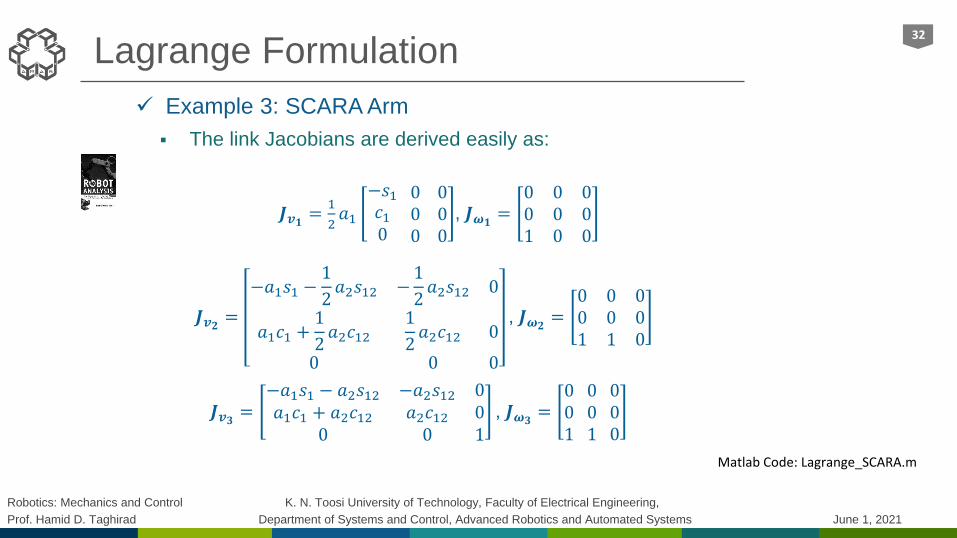
Lagrange Formulation
Example 3: SCARA Arm
The link Jacobians are derived easily as:
𝑱𝒗𝟏 =1
2𝑎1
−𝑠1𝑐10
000
000
, 𝑱𝝎𝟏=
0 0 00 0 01 0 0
𝑱𝒗𝟐 =
−𝑎1𝑠1 −1
2𝑎2𝑠12 −
1
2𝑎2𝑠12 0
𝑎1𝑐1 +1
2𝑎2𝑐12
1
2𝑎2𝑐12 0
0 0 0
, 𝑱𝝎𝟐=
0 0 00 0 01 1 0
𝑱𝒗𝟑 =−𝑎1𝑠1 − 𝑎2𝑠12 −𝑎2𝑠12 0𝑎1𝑐1 + 𝑎2𝑐12 𝑎2𝑐12 0
0 0 1, 𝑱𝝎𝟑
=001
001
000
32
Matlab Code: Lagrange_SCARA.m
Robotics: Mechanics and Control K. N. Toosi University of Technology, Faculty of Electrical Engineering,
Prof. Hamid D. Taghirad Department of Systems and Control, Advanced Robotics and Automated Systems June 1, 2021
Lagrange Formulation
Example 3: SCARA Arm
The robot Mass Matrix is derived as:
𝑴 𝒒 =
𝑖=1
2
𝑚𝑖 𝑱𝒗𝒊𝑻 𝑱𝒗𝒊+ 𝑱𝝎
𝑻𝒊
𝐶𝐼𝑖 𝑱𝝎𝒊
= 𝑚1
1
3𝑎12 0 0
0 0 00 0 0
+ 𝑚2
𝑎12 + 𝑎1𝑎2𝑐2 +
1
3𝑎22 1
2𝑎1𝑎2𝑐2 +
1
3𝑎22 0
1
2𝑎1𝑎2𝑐2 +
1
3𝑎22 1
3𝑎22 0
0 0 0
+
𝑚3
𝑎12 + 2𝑎1𝑎2𝑐2 + 𝑎2
2 𝑎1𝑎2𝑐2 + 𝑎22 0
𝑎1𝑎2𝑐2 + 𝑎22 𝑎2
2 00 0 1
33
𝑀
=
1
3𝑚1𝑎1
2 +𝑚2 𝑎12 +
1
3𝑎22 + 𝑎1𝑎2𝑐2 +𝑚3 𝑎1
2 + 𝑎22 +
1
12𝑎32 + 2𝑎1𝑎2𝑐2 −𝑚2𝑎2
1
3𝑎2 +
1
2𝑎1𝑐2 −𝑚3 𝑎2
2 +1
12𝑎32 + 𝑎1𝑎2𝑐2 0
−𝑚2𝑎21
3𝑎2 +
1
2𝑎1𝑐2 −𝑚3 𝑎2
2 +1
12𝑎32 + 𝑎1𝑎2𝑐2
1
3𝑚2𝑎2
2 +𝑚3 𝑎22 +
1
12𝑎32 0
0 0 𝑚3
Matlab Code: Lagrange_SCARA.m

Robotics: Mechanics and Control K. N. Toosi University of Technology, Faculty of Electrical Engineering,
Prof. Hamid D. Taghirad Department of Systems and Control, Advanced Robotics and Automated Systems June 1, 2021
Lagrange Formulation
Example 3: SCARA Arm
The Gravity vector is derived as:
g 𝒒 =00
−𝑚3𝑔
The Coriolis and centrifugal vector is derived as:
v 𝒒, ሶ𝒒 =
−(𝑚2+2𝑚3)𝑎1𝑎2𝑠2 ሶ𝜃1 ሶ𝜃2 +1
2ሶ𝜃22
1
2𝑚2 +𝑚3 𝑎1𝑎2𝑠2 ሶ𝜃1
2
0
The Lagrange equations is formulated by:
𝐐 =
𝜏1𝜏2𝑓3
= 𝑴 𝒒 ሷ𝒒 + v 𝒒, ሶ𝒒 + g 𝒒 .
34
Matlab Code: Lagrange_SCARA.m
Robotics: Mechanics and Control K. N. Toosi University of Technology, Faculty of Electrical Engineering,
Prof. Hamid D. Taghirad Department of Systems and Control, Advanced Robotics and Automated Systems June 1, 2021
Lagrange Formulation
Example 3: SCARA Arm
The Lagrange equations is formulated by:
𝑴 𝒒 ሷ𝒒 + v 𝒒, ሶ𝒒 + g 𝒒 = 𝑸
35
𝑓3Matlab Code: Lagrange_SCARA.m
Robotics: Mechanics and Control K. N. Toosi University of Technology, Faculty of Electrical Engineering,
Prof. Hamid D. Taghirad Department of Systems and Control, Advanced Robotics and Automated Systems June 1, 2021
Scientist Bio36
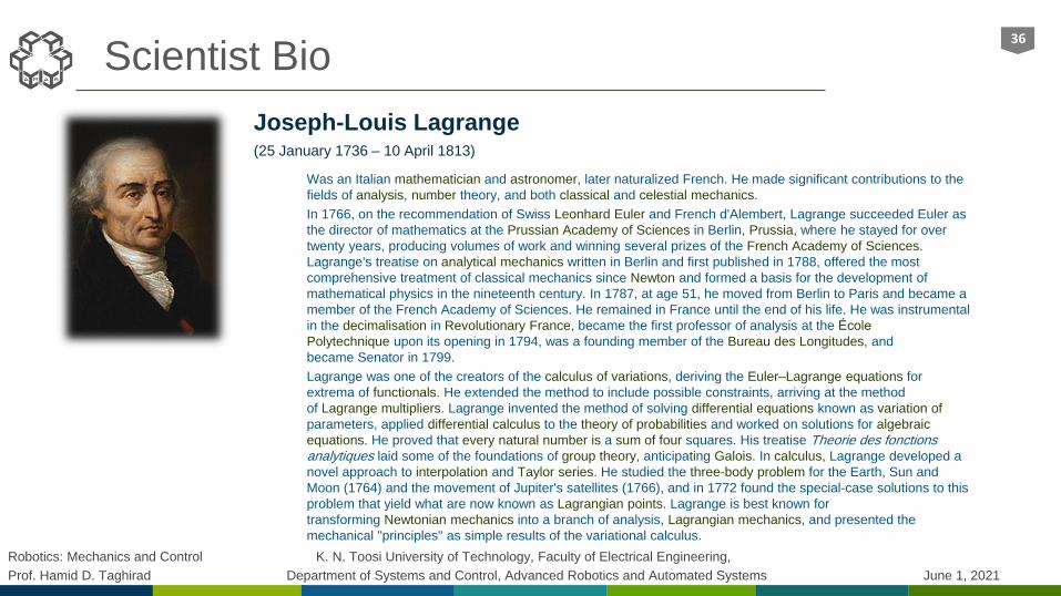
Joseph-Louis Lagrange(25 January 1736 – 10 April 1813)
Was an Italian mathematician and astronomer, later naturalized French. He made significant contributions to the
fields of analysis, number theory, and both classical and celestial mechanics.
In 1766, on the recommendation of Swiss Leonhard Euler and French d'Alembert, Lagrange succeeded Euler as
the director of mathematics at the Prussian Academy of Sciences in Berlin, Prussia, where he stayed for over
twenty years, producing volumes of work and winning several prizes of the French Academy of Sciences.
Lagrange's treatise on analytical mechanics written in Berlin and first published in 1788, offered the most
comprehensive treatment of classical mechanics since Newton and formed a basis for the development of
mathematical physics in the nineteenth century. In 1787, at age 51, he moved from Berlin to Paris and became a
member of the French Academy of Sciences. He remained in France until the end of his life. He was instrumental
in the decimalisation in Revolutionary France, became the first professor of analysis at the École
Polytechnique upon its opening in 1794, was a founding member of the Bureau des Longitudes, and
became Senator in 1799.
Lagrange was one of the creators of the calculus of variations, deriving the Euler–Lagrange equations for
extrema of functionals. He extended the method to include possible constraints, arriving at the method
of Lagrange multipliers. Lagrange invented the method of solving differential equations known as variation of
parameters, applied differential calculus to the theory of probabilities and worked on solutions for algebraic
equations. He proved that every natural number is a sum of four squares. His treatise Theorie des fonctions analytiques laid some of the foundations of group theory, anticipating Galois. In calculus, Lagrange developed a
novel approach to interpolation and Taylor series. He studied the three-body problem for the Earth, Sun and
Moon (1764) and the movement of Jupiter's satellites (1766), and in 1772 found the special-case solutions to this
problem that yield what are now known as Lagrangian points. Lagrange is best known for
transforming Newtonian mechanics into a branch of analysis, Lagrangian mechanics, and presented the
mechanical "principles" as simple results of the variational calculus.

Robotics: Mechanics and Control K. N. Toosi University of Technology, Faculty of Electrical Engineering,
Prof. Hamid D. Taghirad Department of Systems and Control, Advanced Robotics and Automated Systems June 1, 2021
Contents
In this chapter we review the dynamics analysis for serial robots. First the definition to angular and linear accelerations are given, then mass properties, linear and angular momentums, and kinetic energy of a rigid body in space is defined. Lagrange formulation is given in general form, and dynamics mass matrix, gravity and Coriolis and centrifugal vectors are defined and derived for several case studies. Dynamic formulation properties is given next, then actuator dynamics is elaborated for electrically driven robots with gearbox. Finally, linear regression method is used for dynamics calibration, and model verification methods are elaborated by introducing consistency measure.
37
Actuator DynamicsElectrical actuators, permanent magnet DC motors, servo amplifiers, gearbox, motor-gearbox-load dynamics, motor-gearbox-multiple joint robot,
4
Dynamics CalibrationLinear Regression, linear model with constant gravity, house holder reflection, varying gravity term, filtered velocity, model verification, consistency measure.
5
PreliminariesAngular acceleration, linear acceleration of a point, mass properties, center of mass, moments of inertia, inertia matrix transformations, linear and angular momentum, kinetic energy.
1
Lagrange FormulationMotivating example, generalized coordinates and forces, kinetic energy, mass matrix, potential energy, gravity vector, Coriolis and centrifugal vector, case studies.
2
Dynamic Formulation PropertiesMass matrix properties, linearity in parameters, Christoffel Matrix, skew-symmetric property, general dynamic formulation, passivity,
3
Robotics: Mechanics and Control K. N. Toosi University of Technology, Faculty of Electrical Engineering,
Prof. Hamid D. Taghirad Department of Systems and Control, Advanced Robotics and Automated Systems June 1, 2021
Dynamic Formulation Properties
• Dynamics Formulation Representation
𝑴 𝒒 ሷ𝒒 + v 𝒒, ሶ𝒒 + g 𝒒 = 𝑸
Mass Matrix Properties
Since the mass matrix is defined from kinetic energy: 𝐾 =1
2ሶ𝒒𝑇𝑴 𝒒 ሶ𝒒
It is always symmetric and positive definite (∀ Configurations 𝒒)
It is always invertible
It has upper and lower bound
𝜆 𝑰𝑛×𝑛 ≤ 𝑴 𝒒 ≤ ҧ𝜆 𝑰𝑛×𝑛
Furthermore,
1
ഥ𝜆𝑰𝑛×𝑛 ≤ 𝑴−𝟏 𝒒 ≤
1
𝜆𝑰𝑛×𝑛
The bounds may be represented by matrix norm
𝑀 ≤ 𝑴 𝒒 ≤ ഥ𝑀
In which 𝑀 and ഥ𝑀 are positive constants.
38
Robotics: Mechanics and Control K. N. Toosi University of Technology, Faculty of Electrical Engineering,
Prof. Hamid D. Taghirad Department of Systems and Control, Advanced Robotics and Automated Systems June 1, 2021
Dynamic Formulation Properties
• Linearity in Parameters
𝑴 𝒒 ሷ𝒒 + v 𝒒, ሶ𝒒 + g 𝒒 = 𝑸
This formulation is nonlinear and multivariable w.r.t 𝒒
But It could be written in linear regression form w.r.t kinematic and dynamic
parameters
𝑴 𝒒 ሷ𝒒 + v 𝒒, ሶ𝒒 + 𝒈 𝒒 = 𝓨 𝒒, ሶ𝒒, ሷ𝒒 𝚽
In which, 𝓨 denote the linear regressor form
While 𝚽 denote the kinematic and dynamic parameter vector
This regression form is not unique
But could be found for any serial robot
The minimum number of parameters may found by inspection
Or calibration process and singular values decomposition
39
Robotics: Mechanics and Control K. N. Toosi University of Technology, Faculty of Electrical Engineering,
Prof. Hamid D. Taghirad Department of Systems and Control, Advanced Robotics and Automated Systems June 1, 2021
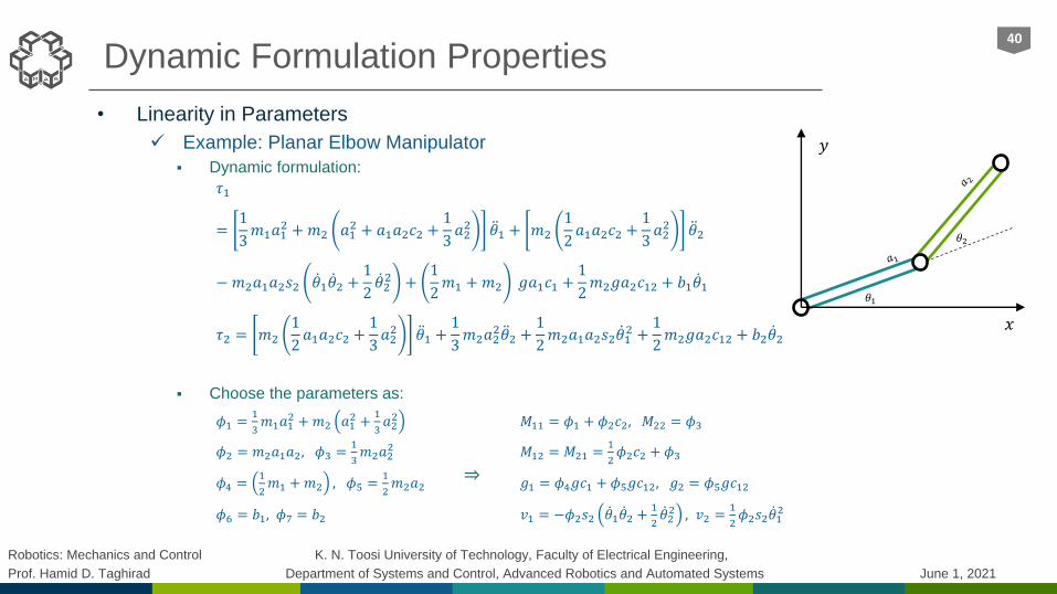
Dynamic Formulation Properties
• Linearity in Parameters
Example: Planar Elbow Manipulator
Dynamic formulation:
𝜏1
=1
3𝑚1𝑎1
2 +𝑚2 𝑎12 + 𝑎1𝑎2𝑐2 +
1
3𝑎22 ሷ𝜃1 + 𝑚2
1
2𝑎1𝑎2𝑐2 +
1
3𝑎22 ሷ𝜃2
−𝑚2𝑎1𝑎2𝑠2 ሶ𝜃1 ሶ𝜃2 +1
2ሶ𝜃22 +
1
2𝑚1 +𝑚2 𝑔𝑎1𝑐1 +
1
2𝑚2𝑔𝑎2𝑐12 + 𝑏1 ሶ𝜃1
𝜏2 = 𝑚2
1
2𝑎1𝑎2𝑐2 +
1
3𝑎22 ሷ𝜃1 +
1
3𝑚2𝑎2
2 ሷ𝜃2 +1
2𝑚2𝑎1𝑎2𝑠2 ሶ𝜃1
2 +1
2𝑚2𝑔𝑎2𝑐12 + 𝑏2 ሶ𝜃2
Choose the parameters as:
𝜙1 =1
3𝑚1𝑎1
2 +𝑚2 𝑎12 +
1
3𝑎22 𝑀11 = 𝜙1 + 𝜙2𝑐2, 𝑀22 = 𝜙3
𝜙2 = 𝑚2𝑎1𝑎2, 𝜙3 =1
3𝑚2𝑎2
2 𝑀12 = 𝑀21 =1
2𝜙2𝑐2 + 𝜙3
𝜙4 =1
2𝑚1 +𝑚2 , 𝜙5 =
1
2𝑚2𝑎2 𝑔1 = 𝜙4𝑔𝑐1 + 𝜙5𝑔𝑐12, 𝑔2 = 𝜙5𝑔𝑐12
𝜙6 = 𝑏1, 𝜙7 = 𝑏2 𝑣1 = −𝜙2𝑠2 ሶ𝜃1 ሶ𝜃2 +1
2ሶ𝜃22 , 𝑣2 =
1
2𝜙2𝑠2 ሶ𝜃1
2
40
⇒
𝑥
𝑦
𝜃1
𝜃2
Robotics: Mechanics and Control K. N. Toosi University of Technology, Faculty of Electrical Engineering,
Prof. Hamid D. Taghirad Department of Systems and Control, Advanced Robotics and Automated Systems June 1, 2021
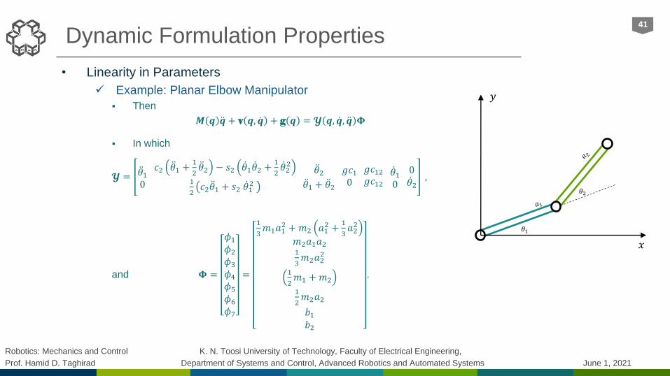
Dynamic Formulation Properties
• Linearity in Parameters
Example: Planar Elbow Manipulator
Then
𝑴 𝒒 ሷ𝒒 + v 𝒒, ሶ𝒒 + g 𝒒 = 𝓨 𝒒, ሶ𝒒, ሷ𝒒 𝚽
In which
𝓨 =ሷ𝜃10
𝑐2 ሷ𝜃1 +1
2ሷ𝜃2 − 𝑠2 ሶ𝜃1 ሶ𝜃2 +
1
2ሶ𝜃22
1
2𝑐2 ሷ𝜃1 + 𝑠2 ሶ𝜃1
2
ሷ𝜃2ሷ𝜃1 + ሷ𝜃2
𝑔𝑐10
𝑔𝑐12𝑔𝑐12
ሶ𝜃10
0ሶ𝜃2
,
and 𝚽 =
𝜙1𝜙2𝜙3𝜙4𝜙5𝜙6𝜙7
=
1
3𝑚1𝑎1
2 +𝑚2 𝑎12 +
1
3𝑎22
𝑚2𝑎1𝑎21
3𝑚2𝑎2
2
1
2𝑚1 +𝑚2
1
2𝑚2𝑎2
𝑏1𝑏2
.
41
𝑥
𝑦
𝜃1
𝜃2
Robotics: Mechanics and Control K. N. Toosi University of Technology, Faculty of Electrical Engineering,
Prof. Hamid D. Taghirad Department of Systems and Control, Advanced Robotics and Automated Systems June 1, 2021
Dynamic Formulation Properties
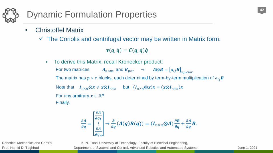
• Christoffel Matrix
The Coriolis and centrifugal vector may be written in Matrix form:
v 𝒒, ሶ𝒒 = 𝑪 𝒒, ሶ𝒒 ሶ𝒒
To derive this Matrix, recall Kronecker product:
For two matrices 𝑨𝑛×𝑚, and 𝑩𝑝×𝑟 → 𝑨⨂𝑩 = 𝑎𝑖𝑗𝑩 𝑛𝑝×𝑚𝑟
The matrix has 𝑝 × 𝑟 blocks, each determined by term-by-term multiplication of 𝑎𝑖𝑗𝑩
Note that 𝑰𝑛×𝑛⨂𝒙 ≠ 𝒙⨂𝑰𝑛×𝑛 but 𝑰𝑛×𝑛⨂𝒙 𝒙 = 𝒙⨂𝑰𝑛×𝑛 𝒙
For any arbitrary 𝒙 ∈ ℝ𝑛
Finally,
𝜕𝑨
𝝏𝒒=
𝜕𝑨
𝝏𝒒𝟏
⋮𝜕𝑨
𝝏𝒒𝒏
→𝝏
𝝏𝒒𝑨 𝒒 𝑩(𝒒) = 𝑰𝑛×𝑛⨂𝑨
𝜕𝑩
𝝏𝒒+
𝜕𝑨
𝝏𝒒𝑩.
42
Robotics: Mechanics and Control K. N. Toosi University of Technology, Faculty of Electrical Engineering,
Prof. Hamid D. Taghirad Department of Systems and Control, Advanced Robotics and Automated Systems June 1, 2021
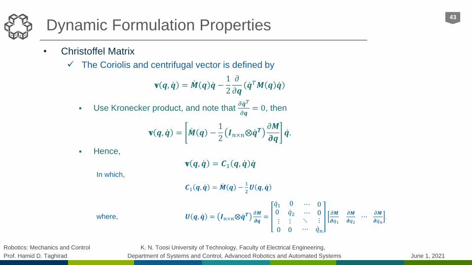
Dynamic Formulation Properties
• Christoffel Matrix
The Coriolis and centrifugal vector is defined by
v 𝒒, ሶ𝒒 = ሶ𝑴 𝒒 ሶ𝒒 −1
2
𝜕
𝜕𝒒ሶ𝒒𝑇𝑴 𝒒 ሶ𝒒
Use Kronecker product, and note that 𝜕 ሶ𝒒𝑇
𝜕𝒒= 0, then
v 𝒒, ሶ𝒒 = ሶ𝑴 𝒒 −1
2𝑰𝑛×𝑛⨂ ሶ𝒒𝑻
𝜕𝑴
𝝏𝒒ሶ𝒒.
Hence,
v 𝒒, ሶ𝒒 = 𝑪1 𝒒, ሶ𝒒 ሶ𝒒
In which,
𝑪1 𝒒, ሶ𝒒 = ሶ𝑴 𝒒 −1
2𝑼 𝒒, ሶ𝒒
where, 𝑼 𝒒, ሶ𝒒 = 𝑰𝑛×𝑛⨂ ሶ𝒒𝑻𝜕𝑴
𝝏𝒒=
ሶ𝑞1 00 ሶ𝑞2
⋯ 0⋯ 0
⋮ ⋮0 0
⋱ ⋮⋯ ሶ𝑞𝑛
𝜕𝑴
𝝏𝑞1
𝜕𝑴
𝝏𝑞2⋯
𝜕𝑴
𝝏𝑞𝑛.
43
Robotics: Mechanics and Control K. N. Toosi University of Technology, Faculty of Electrical Engineering,
Prof. Hamid D. Taghirad Department of Systems and Control, Advanced Robotics and Automated Systems June 1, 2021
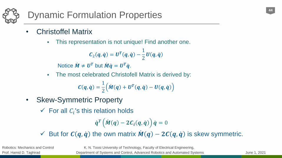
Dynamic Formulation Properties
• Christoffel Matrix
This representation is not unique! Find another one.
𝑪2 𝒒, ሶ𝒒 = 𝑼𝑻 𝒒, ሶ𝒒 −1
2𝑼 𝒒, ሶ𝒒
Notice ሶ𝑴 ≠ 𝑼𝑻 but ሶ𝑴 ሶ𝒒 = 𝑼𝑻 ሶ𝒒.
The most celebrated Christofell Matrix is derived by:
𝑪 𝒒, ሶ𝒒 =1
2ሶ𝑴 𝒒 + 𝑼𝑻 𝒒, ሶ𝒒 − 𝑼 𝒒, ሶ𝒒
• Skew-Symmetric Property
For all 𝐶𝑖 ’s this relation holds
ሶ𝒒𝑻 ሶ𝑴 𝒒 − 𝟐𝑪𝒊 𝒒, ሶ𝒒 ሶ𝒒 = 0
But for 𝑪 𝒒, ሶ𝒒 the own matrix ሶ𝑴 𝒒 − 𝟐𝑪 𝒒, ሶ𝒒 is skew symmetric.
44
Robotics: Mechanics and Control K. N. Toosi University of Technology, Faculty of Electrical Engineering,
Prof. Hamid D. Taghirad Department of Systems and Control, Advanced Robotics and Automated Systems June 1, 2021
Dynamic Formulation Properties
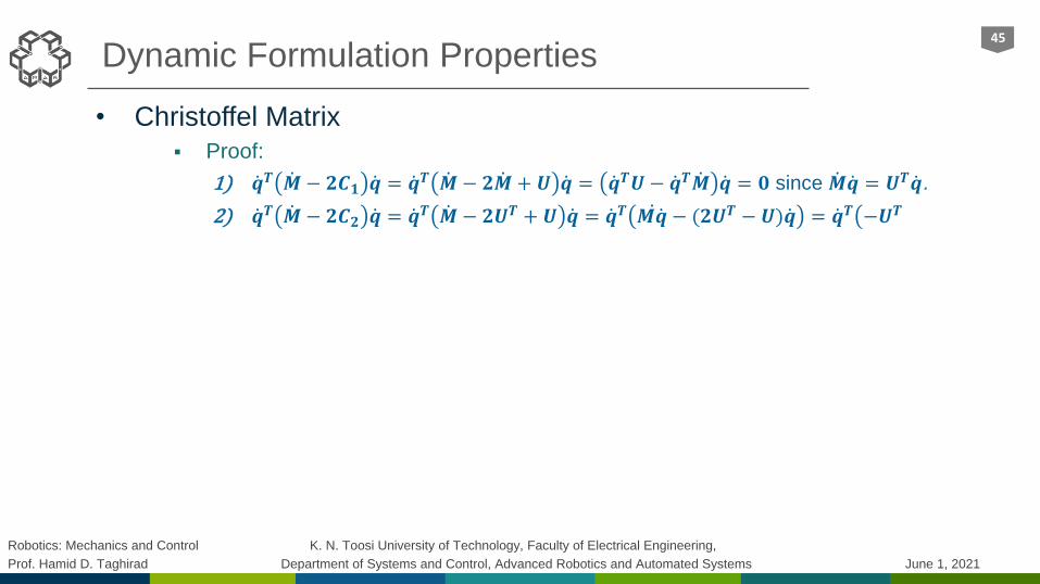
• Christoffel Matrix
Proof:
1) ሶ𝒒𝑻 ሶ𝑴 − 𝟐𝑪𝟏 ሶ𝒒 = ሶ𝒒𝑻 ሶ𝑴 − 𝟐 ሶ𝑴 + 𝑼 ሶ𝒒 = ሶ𝒒𝑻𝑼− ሶ𝒒𝑻 ሶ𝑴 ሶ𝒒 = 𝟎 since ሶ𝑴 ሶ𝒒 = 𝑼𝑻 ሶ𝒒.
2) ሶ𝒒𝑻 ሶ𝑴 − 𝟐𝑪𝟐 ሶ𝒒 = ሶ𝒒𝑻 ሶ𝑴 − 𝟐𝑼𝑻 + 𝑼 ሶ𝒒 = ሶ𝒒𝑻 ሶ𝑴 ሶ𝒒 − (𝟐𝑼𝑻 − 𝑼) ሶ𝒒 = ሶ𝒒𝑻൫−𝑼𝑻
45
Robotics: Mechanics and Control K. N. Toosi University of Technology, Faculty of Electrical Engineering,
Prof. Hamid D. Taghirad Department of Systems and Control, Advanced Robotics and Automated Systems June 1, 2021
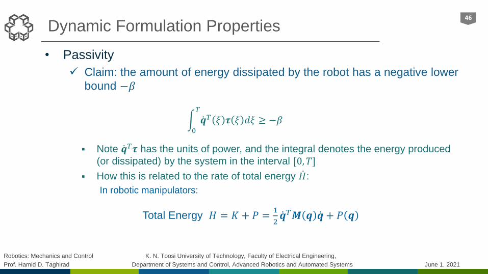
Dynamic Formulation Properties
• Passivity
Claim: the amount of energy dissipated by the robot has a negative lower
bound −𝛽
න0
𝑇
ሶ𝒒𝑇 𝜉 𝝉 𝜉 𝑑𝜉 ≥ −𝛽
Note ሶ𝒒𝑇𝝉 has the units of power, and the integral denotes the energy produced
(or dissipated) by the system in the interval [0, 𝑇]
How this is related to the rate of total energy ሶ𝐻:
In robotic manipulators:
Total Energy 𝐻 = 𝐾 + 𝑃 =1
2ሶ𝒒𝑇𝑴 𝒒 ሶ𝒒 + 𝑃 𝒒
46
Robotics: Mechanics and Control K. N. Toosi University of Technology, Faculty of Electrical Engineering,
Prof. Hamid D. Taghirad Department of Systems and Control, Advanced Robotics and Automated Systems June 1, 2021
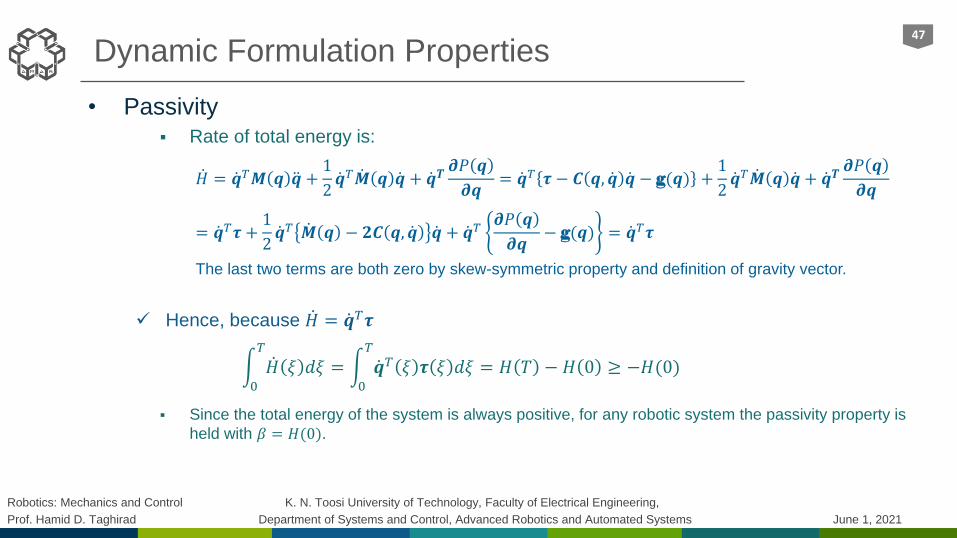
Dynamic Formulation Properties
• Passivity Rate of total energy is:
ሶ𝐻 = ሶ𝒒𝑇𝑴 𝒒 ሷ𝒒 +1
2ሶ𝒒𝑇 ሶ𝑴 𝒒 ሶ𝒒 + ሶ𝒒𝑻
𝝏𝑃 𝒒
𝝏𝒒= ሶ𝒒𝑇 𝝉 − 𝑪 𝒒, ሶ𝒒 ሶ𝒒 − g(𝒒) +
1
2ሶ𝒒𝑇 ሶ𝑴 𝒒 ሶ𝒒 + ሶ𝒒𝑻
𝝏𝑃 𝒒
𝝏𝒒
= ሶ𝒒𝑇𝝉 +1
2ሶ𝒒𝑇 ሶ𝑴 𝒒 − 𝟐𝑪 𝒒, ሶ𝒒 ሶ𝒒 + ሶ𝒒𝑇
𝝏𝑃 𝒒
𝝏𝒒− g(𝒒) = ሶ𝒒𝑇𝝉
The last two terms are both zero by skew-symmetric property and definition of gravity vector.
Hence, because ሶ𝐻 = ሶ𝒒𝑇𝝉
න0
𝑇
ሶ𝐻 𝜉 𝑑𝜉 = න0
𝑇
ሶ𝒒𝑇 𝜉 𝝉 𝜉 𝑑𝜉 = 𝐻 𝑇 − 𝐻 0 ≥ −𝐻(0)
Since the total energy of the system is always positive, for any robotic system the passivity property is
held with 𝛽 = 𝐻(0).
47

Robotics: Mechanics and Control K. N. Toosi University of Technology, Faculty of Electrical Engineering,
Prof. Hamid D. Taghirad Department of Systems and Control, Advanced Robotics and Automated Systems June 1, 2021
Dynamic Simulation
• Forward Dynamics
In forward dynamics given the actuator forces
applied to the robot, the resulting output
trajectory of the robot is found.
General Dynamics:
𝝉 + 𝝉𝒅 = 𝑴 𝒒 ሷ𝒒 + 𝑪 𝒒, ሶ𝒒 ሶ𝒒 + g 𝒒
The Dynamics equations shall be integrated to find the trajectory
The mass matrix is positive definite, hence it is invertible in all configurations
ሷ𝒒 = 𝑴−𝟏 𝒒 𝝉 + 𝝉𝒅 − 𝑪 𝒒, ሶ𝒒 ሶ𝒒 − g 𝒒
Use numerical integration like Runge-Kutta method (ode45 in Matlab or Simulink)
Given the torques 𝝉, 𝝉𝒅 and the initial conditions for the augmented states 𝒙 = 𝒙𝟏, 𝒙𝟐𝑻 = 𝒒, ሶ𝒒 𝑻, use
numerical integration to solve for the trajectory.
ሶ𝒙1 = ሶ𝒒 = 𝒙2
ሶ𝒙2 = ሷ𝒒 = 𝑴−𝟏 𝒙1 𝝉 + 𝝉𝒅 − 𝑪 𝒙𝟏, 𝒙𝟐 𝒙𝟐 − g 𝒙𝟏
48
Forward Dynamics𝒒𝝉
𝝉𝐝
Actuator Torques
Output Trajectory
Disturbance torque
Robotics: Mechanics and Control K. N. Toosi University of Technology, Faculty of Electrical Engineering,
Prof. Hamid D. Taghirad Department of Systems and Control, Advanced Robotics and Automated Systems June 1, 2021
Dynamic Simulation
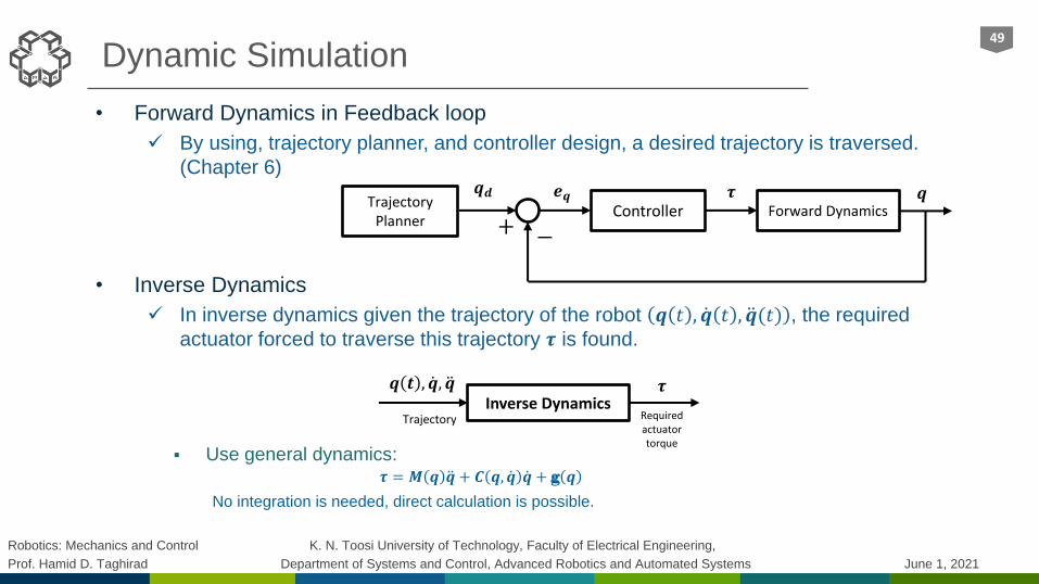
• Forward Dynamics in Feedback loop
By using, trajectory planner, and controller design, a desired trajectory is traversed.
(Chapter 6)
• Inverse Dynamics
In inverse dynamics given the trajectory of the robot 𝒒 𝑡 , ሶ𝒒 𝑡 , ሷ𝒒(𝑡) , the required
actuator forced to traverse this trajectory 𝝉 is found.
Use general dynamics: 𝝉 = 𝑴 𝒒 ሷ𝒒 + 𝑪 𝒒, ሶ𝒒 ሶ𝒒 + g 𝒒
No integration is needed, direct calculation is possible.
49
𝒒𝒅Forward DynamicsController
𝒒𝒆𝒒 𝝉
+ −
Trajectory Planner
Inverse Dynamics𝒒 𝒕 , ሶ𝒒, ሷ𝒒 𝝉
Trajectory Required actuator torque

Robotics: Mechanics and Control K. N. Toosi University of Technology, Faculty of Electrical Engineering,
Prof. Hamid D. Taghirad Department of Systems and Control, Advanced Robotics and Automated Systems June 1, 2021
Contents
In this chapter we review the dynamics analysis for serial robots. First the definition to angular and linear accelerations are given, then mass properties, linear and angular momentums, and kinetic energy of a rigid body in space is defined. Lagrange formulation is given in general form, and dynamics mass matrix, gravity and Coriolis and centrifugal vectors are defined and derived for several case studies. Dynamic formulation properties is given next, then actuator dynamics is elaborated for electrically driven robots with gearbox. Finally, linear regression method is used for dynamics calibration, and model verification methods are elaborated by introducing consistency measure.
50
Actuator DynamicsElectrical actuators, permanent magnet DC motors, servo amplifiers, gearbox, motor-gearbox-load dynamics, motor-gearbox-multiple joint robot,
4
Dynamics CalibrationLinear Regression, linear model with constant gravity, house holder reflection, varying gravity term, filtered velocity, model verification, consistency measure.
5
PreliminariesAngular acceleration, linear acceleration of a point, mass properties, center of mass, moments of inertia, inertia matrix transformations, linear and angular momentum, kinetic energy.
1
Lagrange FormulationMotivating example, generalized coordinates and forces, kinetic energy, mass matrix, potential energy, gravity vector, Coriolis and centrifugal vector, case studies.
2
Dynamic Formulation PropertiesMass matrix properties, linearity in parameters, Christoffel Matrix, skew-symmetric property, general dynamic formulation, passivity,
3
Robotics: Mechanics and Control K. N. Toosi University of Technology, Faculty of Electrical Engineering,
Prof. Hamid D. Taghirad Department of Systems and Control, Advanced Robotics and Automated Systems June 1, 2021
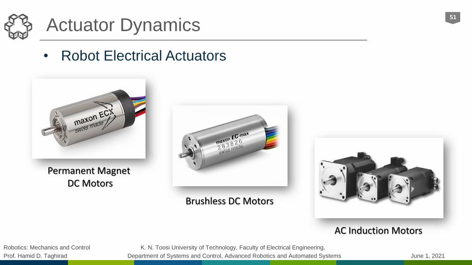
Actuator Dynamics
• Robot Electrical Actuators
51
Permanent MagnetDC Motors
Brushless DC Motors
AC Induction Motors

Robotics: Mechanics and Control K. N. Toosi University of Technology, Faculty of Electrical Engineering,
Prof. Hamid D. Taghirad Department of Systems and Control, Advanced Robotics and Automated Systems June 1, 2021
Actuator Dynamics
• DC Motors
Principle of operation
A current carrying conductor in a magnetic field
experiences a Force
𝐹 = 𝑖 × 𝜙
𝑖: the current in the conductor, 𝜙: the magnetic field flux
DC motor consists of
A fixed Stator (Permanent magnet)
A rotating rotor (Armature)
A commutator: to switch the direction of current
The torque generated in the motor
𝜏𝑚 = 𝐾1𝜙𝑖𝑎𝑖𝑎: the armature current, 𝜙: the magnetic field flux
Lenz’s Law: back-emf voltage
𝑉𝑏 = 𝐾2𝜙𝜔𝑚𝜔𝑚: the angular velocity of the rotor, 𝜙: the magnetic field flux
52

Robotics: Mechanics and Control K. N. Toosi University of Technology, Faculty of Electrical Engineering,
Prof. Hamid D. Taghirad Department of Systems and Control, Advanced Robotics and Automated Systems June 1, 2021
Actuator Dynamics
• DC Motors
Principle of operation
For a permanent magnet DC motor 𝜙 is constant
If SI unit is used:
𝜏𝑚 = 𝐾𝑚𝑖𝑎 and 𝑉𝑏 = 𝐾𝑚𝜔𝑚
𝐾𝑚: the DC motor torque or velocity constant
Electrical model of the PMDC motor
𝐿𝑑𝑖𝑎
𝑑𝑡+ 𝑅𝑖𝑎 + 𝑉𝑏 = 𝑉 𝑡 or 𝐿𝑠 + 𝑅 𝑖𝑎 = 𝑉 − 𝑉𝑏
𝑖𝑎 =𝑉 − 𝑉𝑏𝐿𝑠 + 𝑅
Electro-mechanical model of the PMDC motor
𝜏𝑚 = 𝐾𝑚𝑖𝑎 = 𝜏𝑚 = 𝐾𝑚𝑉 − 𝐾𝑚𝜔𝑚𝐿𝑠 + 𝑅
53
𝑖𝑎
𝜏𝑚
𝜔𝑚
𝑉𝑏𝑉(𝑡)
Robotics: Mechanics and Control K. N. Toosi University of Technology, Faculty of Electrical Engineering,
Prof. Hamid D. Taghirad Department of Systems and Control, Advanced Robotics and Automated Systems June 1, 2021
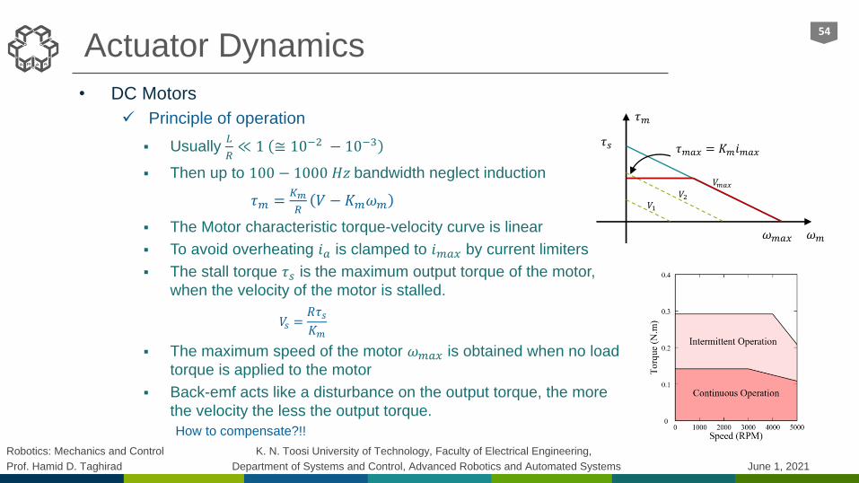
Actuator Dynamics
• DC Motors
Principle of operation
Usually 𝐿
𝑅≪ 1 ≅ 10−2 − 10−3
Then up to 100 − 1000 𝐻𝑧 bandwidth neglect induction
𝜏𝑚 =𝐾𝑚
𝑅𝑉 − 𝐾𝑚𝜔𝑚
The Motor characteristic torque-velocity curve is linear
To avoid overheating 𝑖𝑎 is clamped to 𝑖𝑚𝑎𝑥 by current limiters
The stall torque 𝜏𝑠 is the maximum output torque of the motor,
when the velocity of the motor is stalled.
𝑉𝑠 =𝑅𝜏𝑠𝐾𝑚
The maximum speed of the motor 𝜔𝑚𝑎𝑥 is obtained when no load
torque is applied to the motor
Back-emf acts like a disturbance on the output torque, the more
the velocity the less the output torque.
How to compensate?!!
54
𝜏𝑚
𝑉1
𝑉2
𝑉𝑚𝑎𝑥
𝜔𝑚𝜔𝑚𝑎𝑥
𝜏𝑠 𝜏𝑚𝑎𝑥 = 𝐾𝑚𝑖𝑚𝑎𝑥
Robotics: Mechanics and Control K. N. Toosi University of Technology, Faculty of Electrical Engineering,
Prof. Hamid D. Taghirad Department of Systems and Control, Advanced Robotics and Automated Systems June 1, 2021
Actuator Dynamics
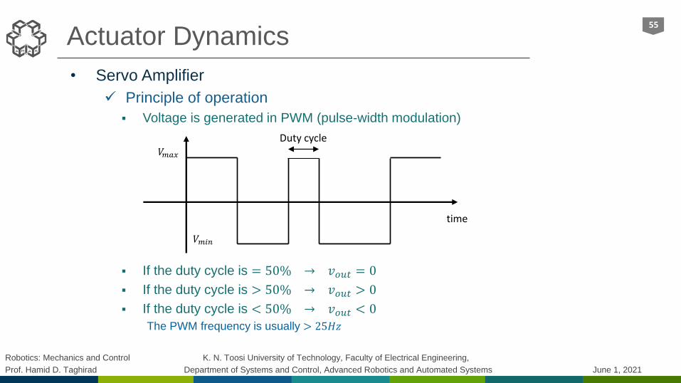
• Servo Amplifier
Principle of operation
Voltage is generated in PWM (pulse-width modulation)
If the duty cycle is = 50% → 𝑣𝑜𝑢𝑡 = 0
If the duty cycle is > 50% → 𝑣𝑜𝑢𝑡 > 0
If the duty cycle is < 50% → 𝑣𝑜𝑢𝑡 < 0
The PWM frequency is usually > 25𝐻𝑧
55
𝑉𝑚𝑎𝑥
𝑉𝑚𝑖𝑛
time
Duty cycle

Robotics: Mechanics and Control K. N. Toosi University of Technology, Faculty of Electrical Engineering,
Prof. Hamid D. Taghirad Department of Systems and Control, Advanced Robotics and Automated Systems June 1, 2021
Actuator Dynamics
• Servo Amplifier
Principle of operation
Current (Torque) mode
An internal current feedback with a tuned PI controller
Ideally considered as a current (torque) source
Back-emf effect limits the performance up to 100 𝐻𝑧 bandwidth
Command signal 𝑖𝑑 is tracked within the bandwidth
Velocity (Voltage) Mode
An external tacho (or velocity) feedback with a tuned lead controller
Command signal 𝜔𝑑 is tracked within the bandwidth when switched to this mode
Current limiter with current foldback
Usually ±𝑖𝑚𝑎𝑥 at continuous operation while permitting higher current intermittently
FWD and REV current clamp
56
Robotics: Mechanics and Control K. N. Toosi University of Technology, Faculty of Electrical Engineering,
Prof. Hamid D. Taghirad Department of Systems and Control, Advanced Robotics and Automated Systems June 1, 2021
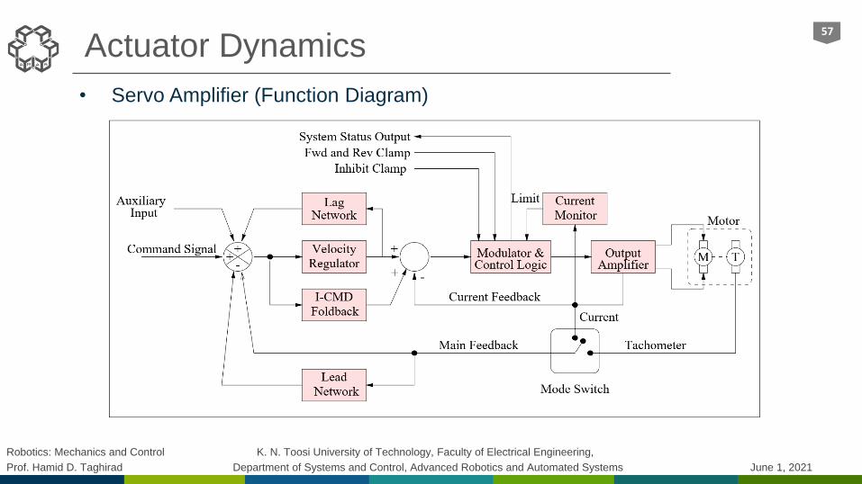
Actuator Dynamics
• Servo Amplifier (Function Diagram)
57
Robotics: Mechanics and Control K. N. Toosi University of Technology, Faculty of Electrical Engineering,
Prof. Hamid D. Taghirad Department of Systems and Control, Advanced Robotics and Automated Systems June 1, 2021
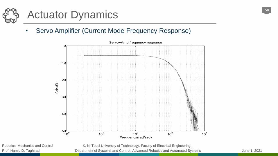
Actuator Dynamics
• Servo Amplifier (Current Mode Frequency Response)
58
Robotics: Mechanics and Control K. N. Toosi University of Technology, Faculty of Electrical Engineering,
Prof. Hamid D. Taghirad Department of Systems and Control, Advanced Robotics and Automated Systems June 1, 2021
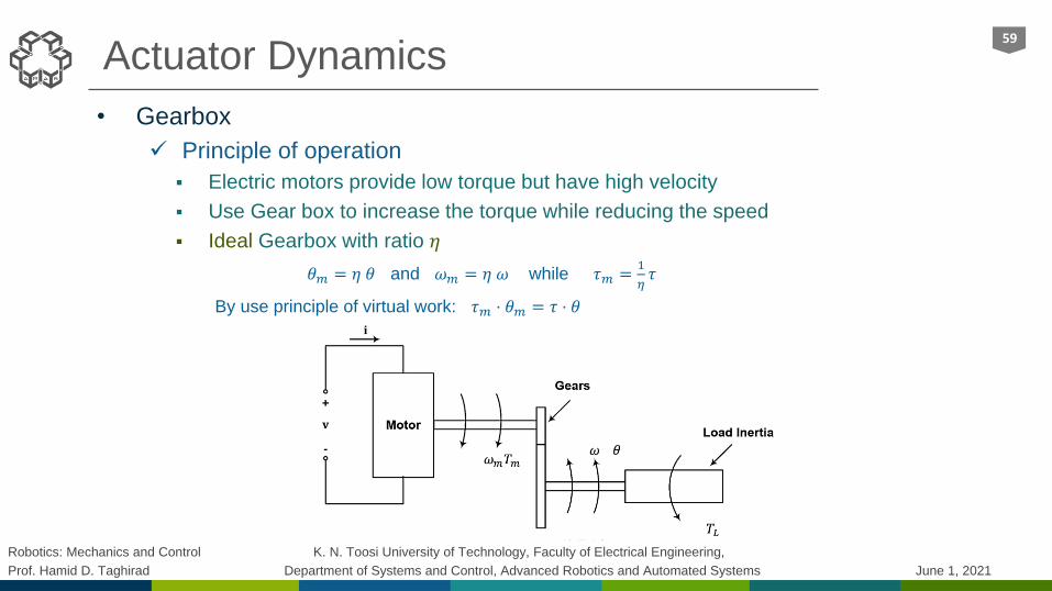
Actuator Dynamics
• Gearbox
Principle of operation
Electric motors provide low torque but have high velocity
Use Gear box to increase the torque while reducing the speed
Ideal Gearbox with ratio 𝜂
𝜃𝑚 = 𝜂 𝜃 and 𝜔𝑚 = 𝜂 𝜔 while 𝜏𝑚 =1
𝜂𝜏
By use principle of virtual work: 𝜏𝑚 ⋅ 𝜃𝑚 = 𝜏 ⋅ 𝜃
59
Robotics: Mechanics and Control K. N. Toosi University of Technology, Faculty of Electrical Engineering,
Prof. Hamid D. Taghirad Department of Systems and Control, Advanced Robotics and Automated Systems June 1, 2021
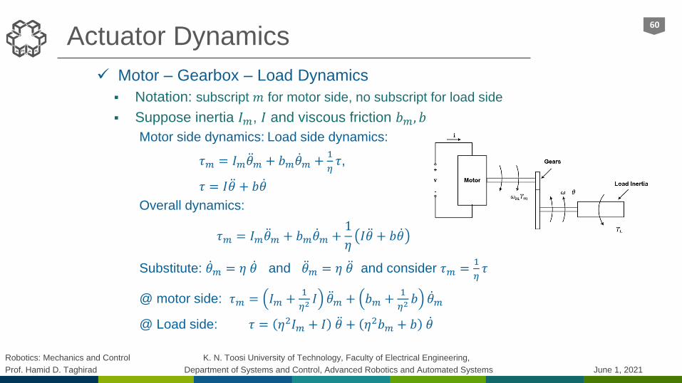
Actuator Dynamics
Motor – Gearbox – Load Dynamics
Notation: subscript 𝑚 for motor side, no subscript for load side
Suppose inertia 𝐼𝑚, 𝐼 and viscous friction 𝑏𝑚, 𝑏
Motor side dynamics: Load side dynamics:
𝜏𝑚 = 𝐼𝑚 ሷ𝜃𝑚 + 𝑏𝑚 ሶ𝜃𝑚 +1
𝜂𝜏,
𝜏 = 𝐼 ሷ𝜃 + 𝑏 ሶ𝜃
Overall dynamics:
𝜏𝑚 = 𝐼𝑚 ሷ𝜃𝑚 + 𝑏𝑚 ሶ𝜃𝑚 +1
𝜂𝐼 ሷ𝜃 + 𝑏 ሶ𝜃
Substitute: ሶ𝜃𝑚 = 𝜂 ሶ𝜃 and ሷ𝜃𝑚 = 𝜂 ሷ𝜃 and consider 𝜏𝑚 =1
𝜂𝜏
@ motor side: 𝜏𝑚 = 𝐼𝑚 +1
𝜂2𝐼 ሷ𝜃𝑚 + 𝑏𝑚 +
1
𝜂2𝑏 ሶ𝜃𝑚
@ Load side: 𝜏 = 𝜂2𝐼𝑚 + 𝐼 ሷ𝜃 + 𝜂2𝑏𝑚 + 𝑏 ሶ𝜃
60
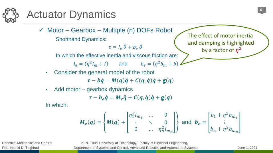
Robotics: Mechanics and Control K. N. Toosi University of Technology, Faculty of Electrical Engineering,
Prof. Hamid D. Taghirad Department of Systems and Control, Advanced Robotics and Automated Systems June 1, 2021
The effect of motor inertia and damping is highlighted
by a factor of 𝜂2
Actuator Dynamics
Motor – Gearbox – Multiple (n) DOFs Robot
Shorthand Dynamics:
𝜏 = 𝐼𝑒 ሷ𝜃 + 𝑏𝑒 ሶ𝜃
In which the effective inertia and viscous friction are:
𝐼𝑒 = 𝜂2𝐼𝑚 + 𝐼 and 𝑏𝑒 = 𝜂2𝑏𝑚 + 𝑏
Consider the general model of the robot
𝝉 − 𝒃 ሶ𝒒 = 𝑴 𝒒 ሷ𝒒 + 𝑪 𝒒, ሶ𝒒 ሶ𝒒 + g 𝒒
Add motor – gearbox dynamics
𝝉 − 𝒃𝒆 ሶ𝒒 = 𝑴𝒆 ሷ𝒒 + 𝑪 𝒒, ሶ𝒒 ሶ𝒒 + g 𝒒
In which:
𝑴𝒆 𝒒 = 𝑴 𝒒 +
𝜂12𝐼𝑚1
… 0
⋮ ⋱ 00 … 𝜂𝑛
2𝐼𝑚𝑛
and 𝒃𝒆 =
𝑏1 + 𝜂2𝑏𝑚1
⋮𝑏𝑛 + 𝜂2𝑏𝑚𝑛
61
Robotics: Mechanics and Control K. N. Toosi University of Technology, Faculty of Electrical Engineering,
Prof. Hamid D. Taghirad Department of Systems and Control, Advanced Robotics and Automated Systems June 1, 2021
Actuator Dynamics
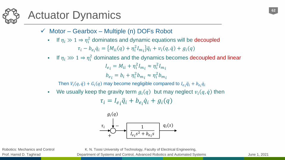
Motor – Gearbox – Multiple (n) DOFs Robot
If 𝜂𝑖 ≫ 1 ⇒ 𝜂𝑖2 dominates and dynamic equations will be decoupled
𝜏𝑖 − 𝑏𝑒𝑖 ሶ𝑞𝑖 = 𝑀𝑖𝑖 𝑞 + 𝜂𝑖2𝐼𝑚𝑖
ሷ𝑞𝑖 + 𝑣𝑖 𝑞, ሶ𝑞 + 𝑔𝑖(𝑞)
If 𝜂𝑖 ⋙ 1 ⇒ 𝜂𝑖2 dominates and the dynamics becomes decoupled and linear
𝐼𝑒𝑖 = 𝑀𝑖𝑖 + 𝜂𝑖2𝐼𝑚𝑖
≈ 𝜂𝑖2𝐼𝑚𝑖
𝑏𝑒𝑖 = 𝑏𝑖 + 𝜂𝑖2𝑏𝑚𝑖
≈ 𝜂𝑖2𝑏𝑚𝑖
Then 𝑉𝑖 𝑞, ሶ𝑞 + 𝐺𝑖 𝑞 may become negligible compared to 𝐼𝑒𝑖 ሷ𝑞𝑖 + 𝑏𝑒𝑖 ሶ𝑞𝑖
We usually keep the gravity term 𝑔𝑖 𝑞 but may neglect 𝑣𝑖 𝑞, ሶ𝑞 then
𝜏𝑖 = 𝐼𝑒𝑖 ሷ𝑞𝑖 + 𝑏𝑒𝑖 ሶ𝑞𝑖 + 𝑔𝑖(𝑞)
62
1
𝐼𝑒𝑖𝑠2 + 𝑏𝑒𝑖𝑠
𝑔𝑖 𝑞
+
𝑞𝑖(𝑠)𝜏𝑖 −
Robotics: Mechanics and Control K. N. Toosi University of Technology, Faculty of Electrical Engineering,
Prof. Hamid D. Taghirad Department of Systems and Control, Advanced Robotics and Automated Systems June 1, 2021
Contents
In this chapter we review the dynamics analysis for serial robots. First the definition to angular and linear accelerations are given, then mass properties, linear and angular momentums, and kinetic energy of a rigid body in space is defined. Lagrange formulation is given in general form, and dynamics mass matrix, gravity and Coriolis and centrifugal vectors are defined and derived for several case studies. Dynamic formulation properties is given next, then actuator dynamics is elaborated for electrically driven robots with gearbox. Finally, linear regression method is used for dynamics calibration, and model verification methods are elaborated by introducing consistency measure.
63
Actuator DynamicsElectrical actuators, permanent magnet DC motors, servo amplifiers, gearbox, motor-gearbox-load dynamics, motor-gearbox-multiple joint robot,
4
Dynamics CalibrationLinear Regression, linear model with constant gravity, house holder reflection, varying gravity term, filtered velocity, model verification, consistency measure.
5
PreliminariesAngular acceleration, linear acceleration of a point, mass properties, center of mass, moments of inertia, inertia matrix transformations, linear and angular momentum, kinetic energy.
1
Lagrange FormulationMotivating example, generalized coordinates and forces, kinetic energy, mass matrix, potential energy, gravity vector, Coriolis and centrifugal vector, case studies.
2
Dynamic Formulation PropertiesMass matrix properties, linearity in parameters, Christoffel Matrix, skew-symmetric property, general dynamic formulation, passivity,
3
Robotics: Mechanics and Control K. N. Toosi University of Technology, Faculty of Electrical Engineering,
Prof. Hamid D. Taghirad Department of Systems and Control, Advanced Robotics and Automated Systems June 1, 2021
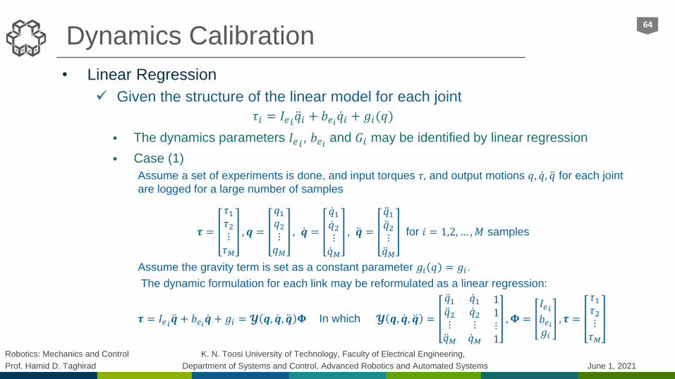
Dynamics Calibration
• Linear Regression
Given the structure of the linear model for each joint
𝜏𝑖 = 𝐼𝑒𝑖 ሷ𝑞𝑖 + 𝑏𝑒𝑖 ሶ𝑞𝑖 + 𝑔𝑖(𝑞)
The dynamics parameters 𝐼𝑒𝑖, 𝑏𝑒𝑖 and 𝐺𝑖 may be identified by linear regression
Case (1)
Assume a set of experiments is done, and input torques 𝜏, and output motions 𝑞, ሶ𝑞, ሷ𝑞 for each joint
are logged for a large number of samples
𝝉 =
𝜏1𝜏2⋮𝜏𝑀
, 𝒒 =
𝑞1𝑞2⋮𝑞𝑀
, ሶ𝒒 =
ሶ𝑞1ሶ𝑞2⋮ሶ𝑞𝑀
, ሷ𝒒 =
ሷ𝑞1ሷ𝑞2⋮ሷ𝑞𝑀
for 𝑖 = 1,2, … ,𝑀 samples
Assume the gravity term is set as a constant parameter 𝑔𝑖 𝑞 = 𝑔𝑖.
The dynamic formulation for each link may be reformulated as a linear regression:
𝝉 = 𝐼𝑒𝑖 ሷ𝒒 + 𝑏𝑒𝑖 ሶ𝒒 + 𝑔𝑖 = 𝓨 𝒒, ሶ𝒒, ሷ𝒒 𝚽 In which 𝓨 𝒒, ሶ𝒒, ሷ𝒒 =
ሷ𝑞1ሷ𝑞2⋮ሷ𝑞𝑀
ሶ𝑞1ሶ𝑞2⋮ሶ𝑞𝑀
11⋮1
,𝚽 =
𝐼𝑒𝑖𝑏𝑒𝑖𝑔𝑖
, 𝝉 =
𝜏1𝜏2⋮𝜏𝑀
64
Robotics: Mechanics and Control K. N. Toosi University of Technology, Faculty of Electrical Engineering,
Prof. Hamid D. Taghirad Department of Systems and Control, Advanced Robotics and Automated Systems June 1, 2021
Dynamics Calibration
• Linear Regression
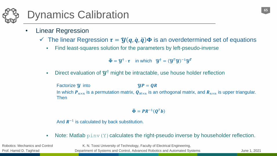
The linear Regression 𝝉 = 𝓨 𝒒, ሶ𝒒, ሷ𝒒 𝚽 is an overdetermined set of equations
Find least-squares solution for the parameters by left-pseudo-inverse
𝚽 = 𝓨† ⋅ 𝝉 in which 𝓨† = 𝓨𝑇𝓨 −1𝓨𝑻
Direct evaluation of 𝓨† might be intractable, use house holder reflection
Factorize 𝓨 into 𝓨𝑷 = 𝑸𝑹
In which 𝑷𝑛×𝑛 is a permutation matrix, 𝑸𝑀×𝑛 is an orthogonal matrix, and 𝑹𝑛×𝑛 is upper triangular.
Then
𝚽 = 𝑷𝑹−1 𝑸𝑇𝒃
And 𝑹−1 is calculated by back substitution.
Note: Matlab pinv(Y)calculates the right-pseudo inverse by householder reflection.
65
Robotics: Mechanics and Control K. N. Toosi University of Technology, Faculty of Electrical Engineering,
Prof. Hamid D. Taghirad Department of Systems and Control, Advanced Robotics and Automated Systems June 1, 2021
Dynamics Calibration
• Linear Regression
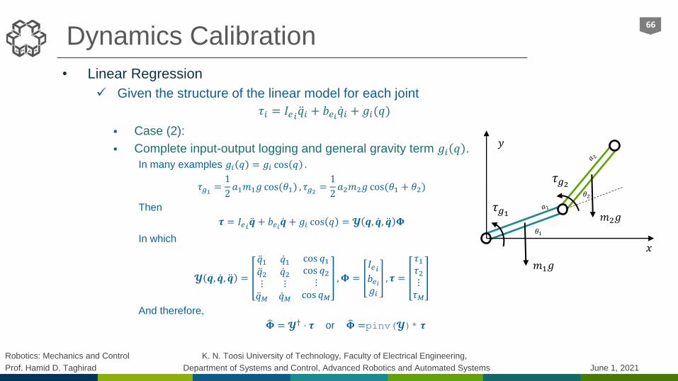
Given the structure of the linear model for each joint
𝜏𝑖 = 𝐼𝑒𝑖 ሷ𝑞𝑖 + 𝑏𝑒𝑖 ሶ𝑞𝑖 + 𝑔𝑖(𝑞)
Case (2):
Complete input-output logging and general gravity term 𝑔𝑖 𝑞 .
In many examples 𝑔𝑖 𝑞 = 𝑔𝑖 cos 𝑞 .
𝜏𝑔1 =1
2𝑎1𝑚1𝑔 cos(𝜃1) , 𝜏𝑔2 =
1
2𝑎2𝑚2𝑔 cos(𝜃1 + 𝜃2)
Then
𝝉 = 𝐼𝑒𝑖 ሷ𝒒 + 𝑏𝑒𝑖 ሶ𝒒 + 𝑔𝑖 cos 𝑞 = 𝓨 𝒒, ሶ𝒒, ሷ𝒒 𝚽
In which
𝓨 𝒒, ሶ𝒒, ሷ𝒒 =
ሷ𝑞1ሷ𝑞2⋮ሷ𝑞𝑀
ሶ𝑞1ሶ𝑞2⋮ሶ𝑞𝑀
cos 𝑞1cos 𝑞2⋮
cos 𝑞𝑀
, 𝚽 =
𝐼𝑒𝑖𝑏𝑒𝑖𝑔𝑖
, 𝝉 =
𝜏1𝜏2⋮𝜏𝑀
And therefore,
𝚽 = 𝓨† ⋅ 𝝉 or 𝚽 =pinv(𝓨)* 𝝉
66
𝑥
𝑦
𝜃1
𝜃2
𝑚1𝑔
𝑚2𝑔𝜏𝑔1
𝜏𝑔2

Robotics: Mechanics and Control K. N. Toosi University of Technology, Faculty of Electrical Engineering,
Prof. Hamid D. Taghirad Department of Systems and Control, Advanced Robotics and Automated Systems June 1, 2021
Dynamics Calibration
• Linear Regression
Given the structure of the linear model for each joint
𝜏𝑖 = 𝐼𝑒𝑖 ሷ𝑞𝑖 + 𝑏𝑒𝑖 ሶ𝑞𝑖 + 𝑔𝑖(𝑞)
Case (3): Only 𝝉 and 𝒒 are measured
Use filtered differentiation
In which
𝜔𝑓 𝐻𝑧 =1
𝜏𝑓is selected such that 10 𝜔𝐵𝑊 < 𝜔𝑓 < 0.1 𝜔𝑛𝑜𝑖𝑠𝑒
Where 𝜔𝐵𝑊 denotes the system bandwidth frequency while 𝜔𝑛𝑜𝑖𝑠𝑒 denotes the major noise
frequency content
Practically 0.001 < 𝜏𝑓 < 0.05 or equivalently 20 < 𝜔𝑓 < 103 would be a good choice.
Use Matlab command filtfilt to remove the delay in the filtered signal
Use the filter twice to find the angular acceleration ሷ𝑞𝑓.
Check the filtered differentiation output and tune 𝜏𝑓 to reduce the output noise.
67
𝑠
𝜏𝑓𝑠 + 1
ሶ𝑞𝑓𝑞
Robotics: Mechanics and Control K. N. Toosi University of Technology, Faculty of Electrical Engineering,
Prof. Hamid D. Taghirad Department of Systems and Control, Advanced Robotics and Automated Systems June 1, 2021
Dynamics Calibration
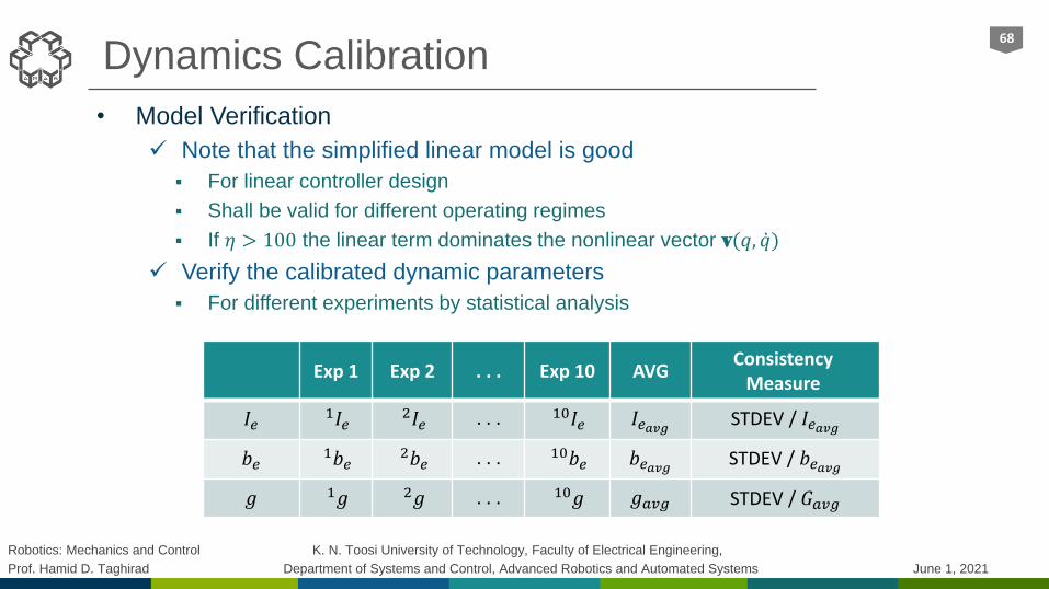
• Model Verification
Note that the simplified linear model is good
For linear controller design
Shall be valid for different operating regimes
If 𝜂 > 100 the linear term dominates the nonlinear vector v(𝑞, ሶ𝑞)
Verify the calibrated dynamic parameters
For different experiments by statistical analysis
68
Consistency Measure
AVGExp 10. . .Exp 2Exp 1
STDEV / 𝐼𝑒𝑎𝑣𝑔𝐼𝑒𝑎𝑣𝑔10𝐼𝑒. . .2𝐼𝑒
1𝐼𝑒𝐼𝑒
STDEV / 𝑏𝑒𝑎𝑣𝑔𝑏𝑒𝑎𝑣𝑔10𝑏𝑒. . .2𝑏𝑒
1𝑏𝑒𝑏𝑒
STDEV / 𝐺𝑎𝑣𝑔𝑔𝑎𝑣𝑔10𝑔. . .2𝑔1𝑔𝑔

Robotics: Mechanics and Control K. N. Toosi University of Technology, Faculty of Electrical Engineering,
Prof. Hamid D. Taghirad Department of Systems and Control, Advanced Robotics and Automated Systems June 1, 2021
Dynamics Calibration
• Model Verification
Verify the calibrated dynamic parameters
For different experiments by statistical analysis
If C.M. < 30% The average parameter is suitable for controller design
If C.M. < 80% The averaged parameters could be used for controller design using
robust linear controllers
If C.M. > 80% Then your model is incomplete and you need to add terms in your
model
If for different experiments the obtained parameters are physically inconsistent
For example you get negative moment of inertia or damping parameters
This means your model is still not good enough for calibration
You may use constrained optimization to add bound on the parameters
Matlab fmincon command may be used in this case.
69
Robotics: Mechanics and Control K. N. Toosi University of Technology, Faculty of Electrical Engineering,
Prof. Hamid D. Taghirad Department of Systems and Control, Advanced Robotics and Automated Systems June 1, 2021
Hamid D. Taghirad has received his B.Sc. degree in mechanical engineering
from Sharif University of Technology, Tehran, Iran, in 1989, his M.Sc. in mechanical
engineering in 1993, and his Ph.D. in electrical engineering in 1997, both
from McGill University, Montreal, Canada. He is currently the University Vice-
Chancellor for Global strategies and International Affairs, Professor and the Director
of the Advanced Robotics and Automated System (ARAS), Department of Systems
and Control, Faculty of Electrical Engineering, K. N. Toosi University of Technology,
Tehran, Iran. He is a senior member of IEEE, and Editorial board of International
Journal of Robotics: Theory and Application, and International Journal of Advanced
Robotic Systems. His research interest is robust and nonlinear control applied to
robotic systems. His publications include five books, and more than 250 papers in
international Journals and conference proceedings.
About Hamid D. Taghirad
Hamid D. TaghiradProfessor
Robotics: Mechanics and Control K. N. Toosi University of Technology, Faculty of Electrical Engineering,
Prof. Hamid D. Taghirad Department of Systems and Control, Advanced Robotics and Automated Systems June 1, 2021
Chapter 5: Dynamic Analysis
To read more and see the course videos visit our course website:
http://aras.kntu.ac.ir/arascourses/robotics/
Thank You
Robotics: Mechanics & Control


![[John J.craig] Introduction to Robotics Mechanics (BookFi.org)](https://static.fdocuments.net/doc/165x107/55cf8ebe550346703b952908/john-jcraig-introduction-to-robotics-mechanics-bookfiorg.jpg)