Robotics 2014 06 Trajectory Planning 1 - polito.it · Trajectory planning TRAJECTORY PLANNER...
58
Trajectory planning Trajectory planning – 1
Transcript of Robotics 2014 06 Trajectory Planning 1 - polito.it · Trajectory planning TRAJECTORY PLANNER...
Trajectory planning Trajectory planning –– 11
Introduction
The robot planning problem can be decomposed into a structured class of interconnected activities, at different hierarchical levels, usually called with different names:
1. Objective: it defines the highest activity level; typically due to the overall scope of the entire process where the robot is present; for example, the assembly of an engine head or moving from A to B while collecting soil samples
2. Task: it defines a subset of actions/operations to be accomplished for the attainment of the objective: for example, the assembly of the engine pistons or the identification of a soil sample and its collection
3. Operation: it defines one of the single activities in which the task is decomposed: for example, the insertion of a piston in the cylinder, or the approach to the soil sample
Basilio Bona - DAUIN - PoliTo 2ROBOTICS 01PEEQW
Introduction
4. Move: it defines a single motion that must be executed to
perform an operation: for example, close the hand to grasp the
piston, move the piston in a predefined position, move the arm
near the sample, attain the right pose.
5. Path/Trajectory: the elementary move is decomposed in one 5. Path/Trajectory: the elementary move is decomposed in one
ore more paths (no defined time law) or trajectories (defined
time law and kinematic constraints).
6. Reference: it consists of the vector of the data obtained
sampling the path/trajectory, supplied to the motors as
references for their controlcontrol: this is represents the action
performed at the most basic level.
Basilio Bona - DAUIN - PoliTo 3ROBOTICS 01PEEQW
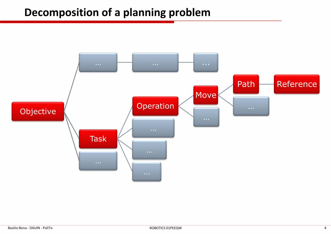
Decomposition of a planning problem
Objective
… … ...
Operation
Move
Path Reference
…
…
Basilio Bona - DAUIN - PoliTo 4ROBOTICS 01PEEQW
Task
…
…
…
…
…
Planning and control
The controlcontrol problem consists in designing the control algorithms for
the robot motors, such that the TCP motion follows a specified path
in the cartesian space. Two types of tasks can be defined:
1. tasks that do not require an interaction with the environment (free
space motion); the manipulator moves its TCP following cartesian
trajectories, with constraint on positions, velocities and accelerations.
Sometimes it is sufficient to move the joints from a specified value to Sometimes it is sufficient to move the joints from a specified value to
another without following a particular geometric path
2. tasks that require and interaction with the environment, i.e., where the
TCP shall move in some cartesian subspace while it applies (or is
subject to) forces or torques to the environment
Only the first type of tasks will be considered
The control may take place at joint level (joint space control) or at
cartesian level (task space control)
Basilio Bona - DAUIN - PoliTo 5ROBOTICS 01PEEQW
Fixed vs mobile robots
� This first part will introduce the planning problems and
algorithms related to fixed (industrial) robotic arms
� Mobile robots path planning will be treated later on
� The two problems are very similar
� The only difference is the kinematic model of the robot and � The only difference is the kinematic model of the robot and
the actuation controls that operate
� on the revolute joints, for robotic arms
� on the wheel motors, for wheeled robots
� on the leg motors, for legged (humanoid and other types of
biomimetic robots)
Basilio Bona - DAUIN - PoliTo 6ROBOTICS 01PEEQW
Industrial RobotsIndustrial Robots
Basilio Bona - DAUIN - PoliTo 7ROBOTICS 01PEEQW
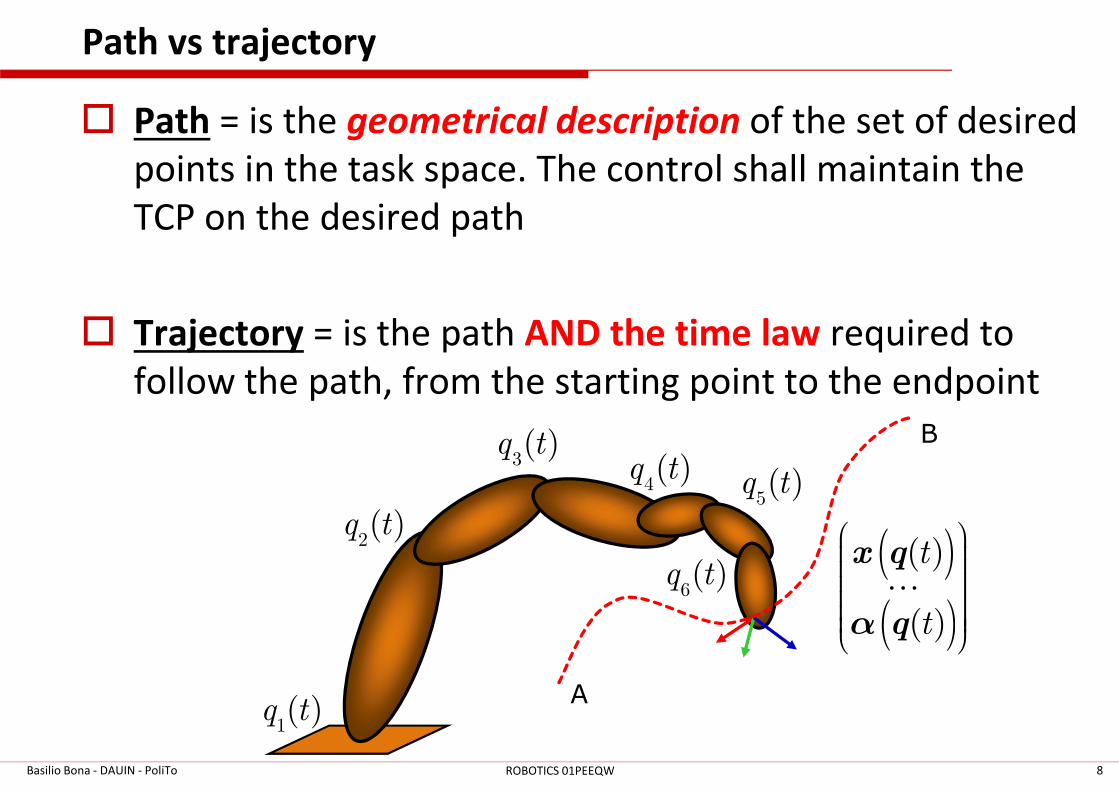
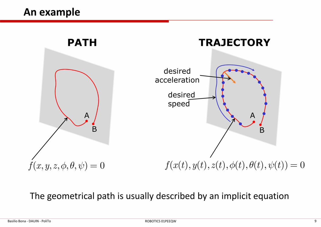
Path vs trajectory
� Path = is the geometrical description of the set of desired
points in the task space. The control shall maintain the
TCP on the desired path
� Trajectory = is the path AND the time law required to
follow the path, from the starting point to the endpoint follow the path, from the starting point to the endpoint
Basilio Bona - DAUIN - PoliTo 8ROBOTICS 01PEEQW
1( )q t
2( )q t
3( )q t
( )
( )
( )
( )
t
t
x q
q⋯
α
4( )q t
5( )q t
6( )q t
A
B
An example
PATH TRAJECTORY
desiredspeed
desiredacceleration
AA
Basilio Bona - DAUIN - PoliTo 9ROBOTICS 01PEEQW
( , , , , , ) 0f x y z φ θ ψ = ( ( ), ( ), ( ), ( ), ( ), ( )) 0f x t y t z t t t tφ θ ψ =
The geometrical path is usually described by an implicit equation
A
B
A
B
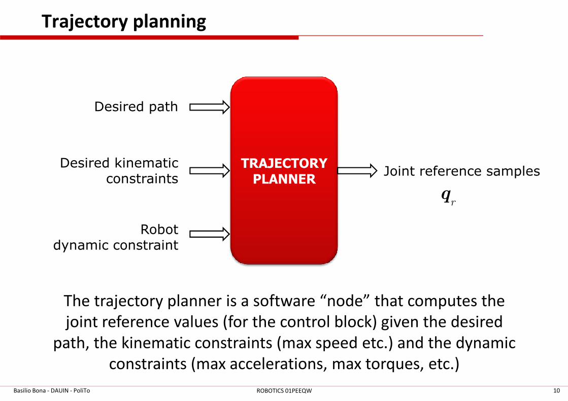
Trajectory planning
TRAJECTORY
PLANNER
Desired path
Desired kinematicconstraints
Joint reference samples
rq
Basilio Bona - DAUIN - PoliTo 10ROBOTICS 01PEEQW
Robotdynamic constraint
The trajectory planner is a software “node” that computes the
joint reference values (for the control block) given the desired
path, the kinematic constraints (max speed etc.) and the dynamic
constraints (max accelerations, max torques, etc.)
rq
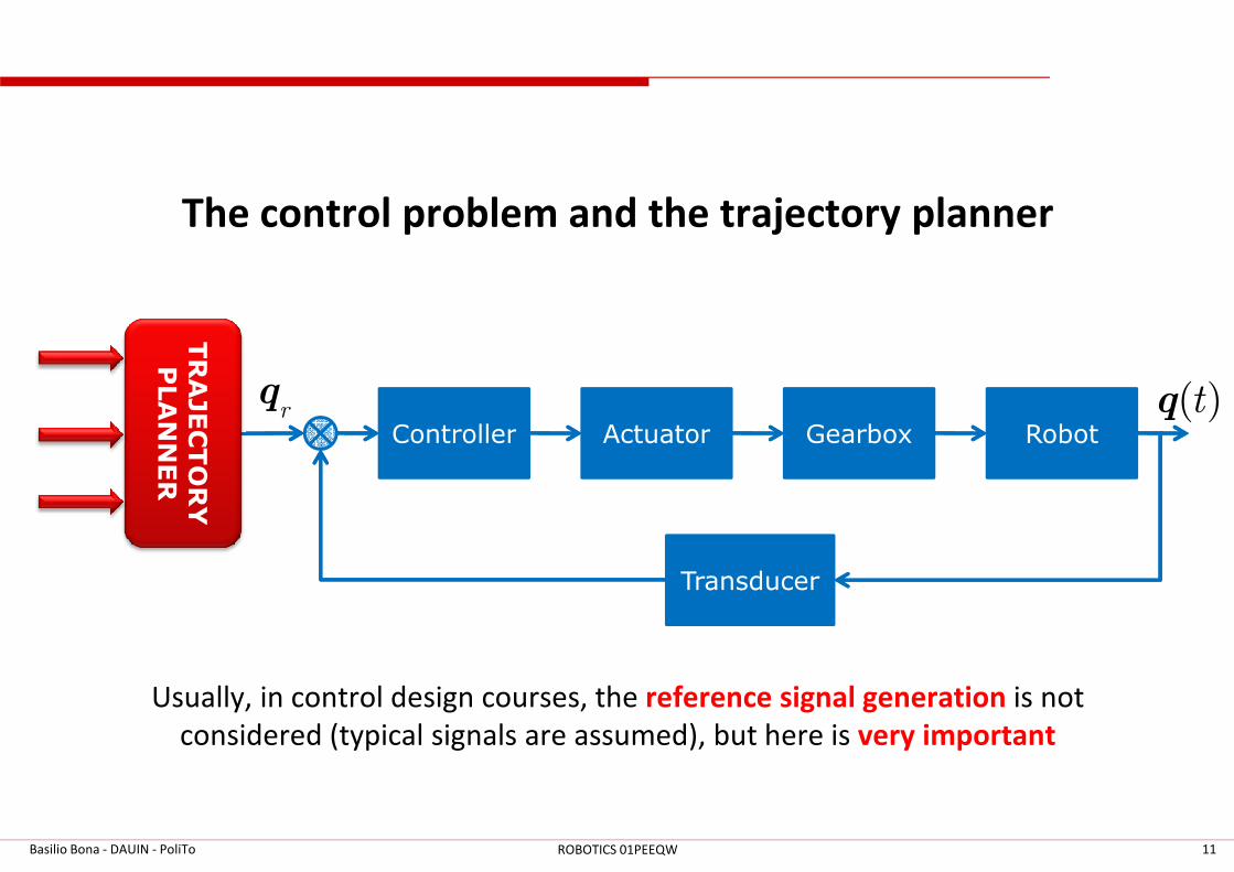
The control problem and the trajectory planner
Controller Actuator Gearbox Robotrq ( )tq
TR
AJEC
TO
RY
PLA
NN
ER
Basilio Bona - DAUIN - PoliTo 11ROBOTICS 01PEEQW
Controller Actuator Gearbox Robot
Transducer
TR
AJEC
TO
RY
PLA
NN
ER
Usually, in control design courses, the reference signal generation is not
considered (typical signals are assumed), but here is very important
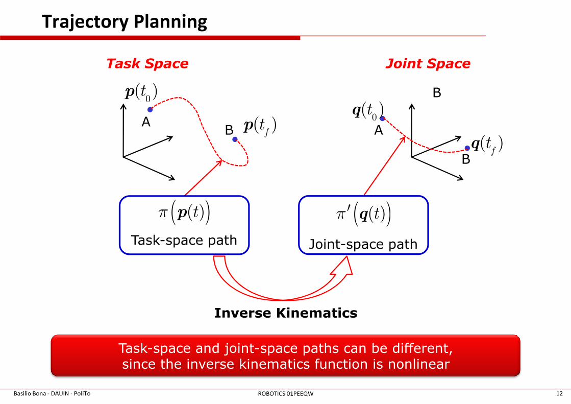
Trajectory Planning
Task Space Joint Space
0( )tp
( )f
tp0
( )tq
( )f
tq
( )( )tπ p ( )′
AB A
B
B
( )( )tπ p
Task-space path
( )( )tπ′ q
Joint-space path
Inverse Kinematics
Basilio Bona - DAUIN - PoliTo 12ROBOTICS 01PEEQW
Task-space and joint-space paths can be different, since the inverse kinematics function is nonlinear
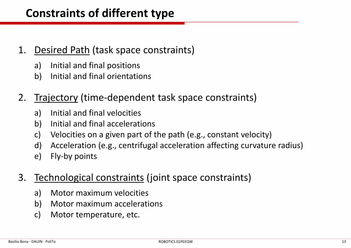
Constraints of different type
1. Desired Path (task space constraints)
a) Initial and final positions
b) Initial and final orientations
2. Trajectory (time-dependent task space constraints)
a) Initial and final velocities
b) Initial and final accelerationsb) Initial and final accelerations
c) Velocities on a given part of the path (e.g., constant velocity)
d) Acceleration (e.g., centrifugal acceleration affecting curvature radius)
e) Fly-by points
3. Technological constraints (joint space constraints)
a) Motor maximum velocities
b) Motor maximum accelerations
c) Motor temperature, etc.
Basilio Bona - DAUIN - PoliTo 13ROBOTICS 01PEEQW
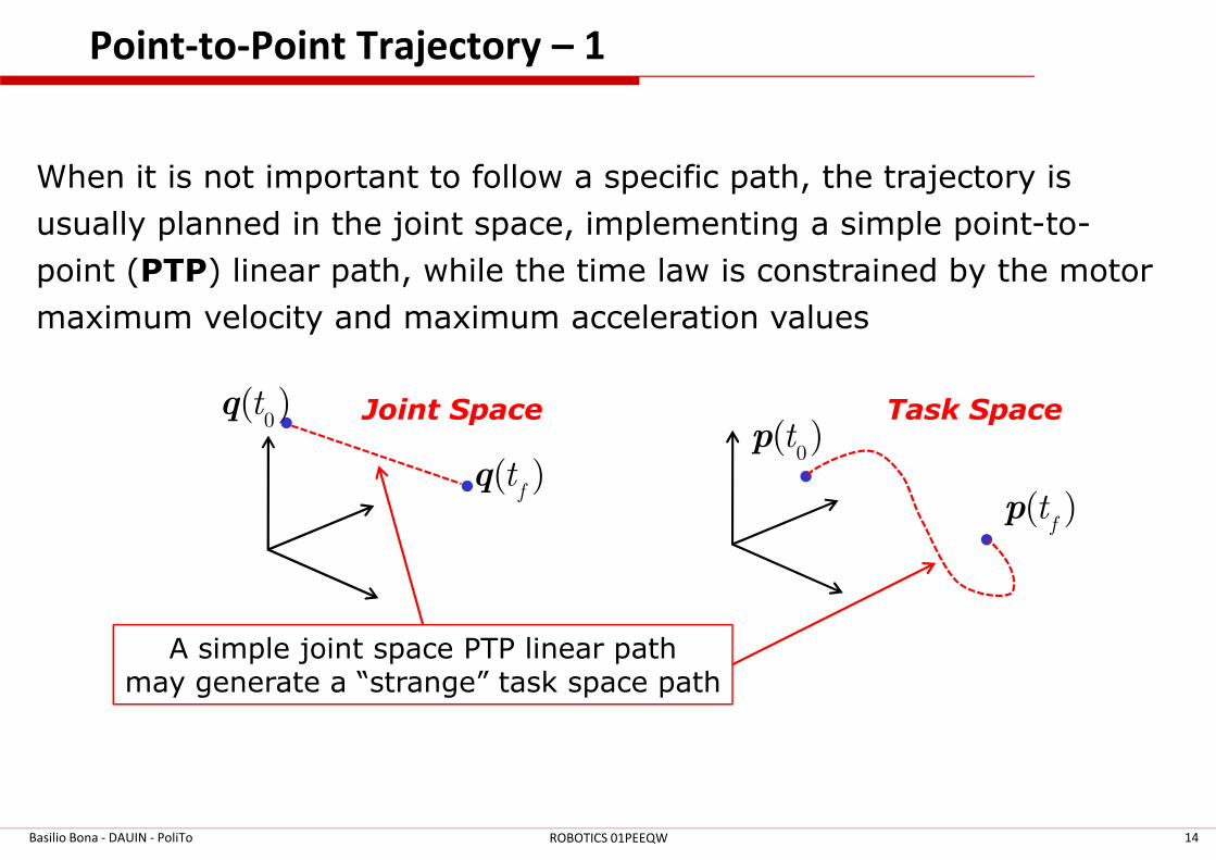
Point-to-Point Trajectory – 1
When it is not important to follow a specific path, the trajectory is
usually planned in the joint space, implementing a simple point-to-
point (PTP) linear path, while the time law is constrained by the motor
maximum velocity and maximum acceleration values
0( )tq Task Space
( )tpJoint Space
A simple joint space PTP linear path may generate a “strange” task space path
0
( )f
tq
Basilio Bona - DAUIN - PoliTo 14ROBOTICS 01PEEQW
0( )tp
( )f
tp
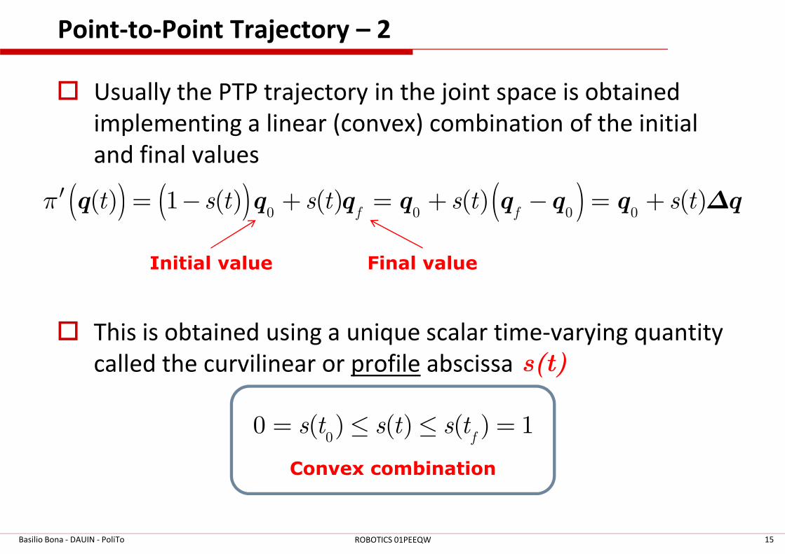
Point-to-Point Trajectory – 2
� Usually the PTP trajectory in the joint space is obtained
implementing a linear (convex) combination of the initial
and final values
( ) ( ) ( )0 0 0 0( ) 1 ( ) ( ) ( ) ( )
f ft s t s t s t s tπ′ = − + = + − = +q q q q q q q q∆
Initial value Final value
Basilio Bona - DAUIN - PoliTo 15ROBOTICS 01PEEQW
00 ( ) ( ) ( ) 1
fs t s t s t= ≤ ≤ =
Convex combination
� This is obtained using a unique scalar time-varying quantity
called the curvilinear or profile abscissa s(t)
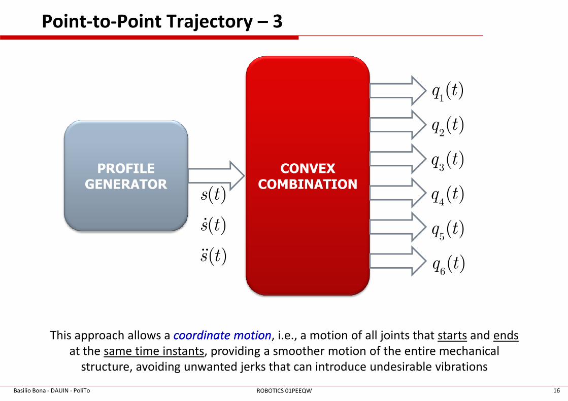
Point-to-Point Trajectory – 3
PROFILE
GENERATOR
CONVEX
COMBINATION( )s t
1( )q t
2( )q t
3( )q t
4( )q t
Basilio Bona - DAUIN - PoliTo 16ROBOTICS 01PEEQW
( )s tɺ
( )s tɺɺ
( )s t4( )q t
5( )q t
6( )q t
This approach allows a coordinate motioncoordinate motion, i.e., a motion of all joints that starts and ends
at the same time instants, providing a smoother motion of the entire mechanical
structure, avoiding unwanted jerks that can introduce undesirable vibrations
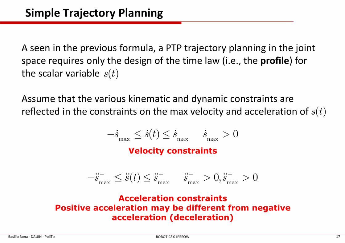
Simple Trajectory Planning
A seen in the previous formula, a PTP trajectory planning in the joint
space requires only the design of the time law (i.e., the profile) for
the scalar variable
Assume that the various kinematic and dynamic constraints are
reflected in the constraints on the max velocity and acceleration of ( )s t
( )s t
Basilio Bona - DAUIN - PoliTo 17ROBOTICS 01PEEQW
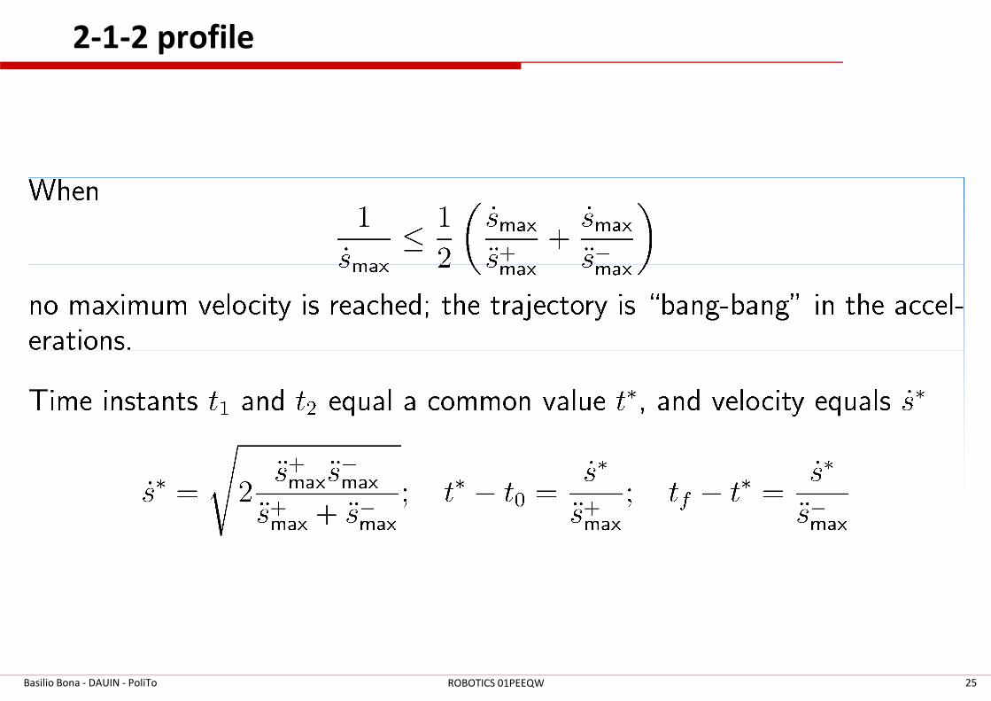
max max max( ) 0s s t s s− ≤ ≤ >ɺ ɺ ɺ ɺ
max max max max( ) 0, 0s s t s s s− + − +− ≤ ≤ > >ɺɺ ɺɺ ɺɺ ɺɺ ɺɺ
Acceleration constraintsPositive acceleration may be different from negative
acceleration (deceleration)
Velocity constraints
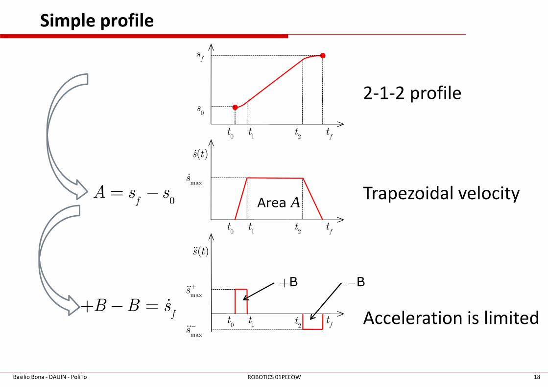
Simple profile
0t
1t
2t
ft
fs
( )s tɺ
maxsɺ
Trapezoidal velocity
2-1-2 profile0
s
AA s s= −
0t
0t
1t
1t
2t
2t
ft
ft
( )s tɺɺ
maxs +ɺɺ
maxs−ɺɺ
Acceleration is limited
Trapezoidal velocityArea A
+B −B
0fA s s= −
fB B s+ − = ɺ
Basilio Bona - DAUIN - PoliTo 18ROBOTICS 01PEEQW
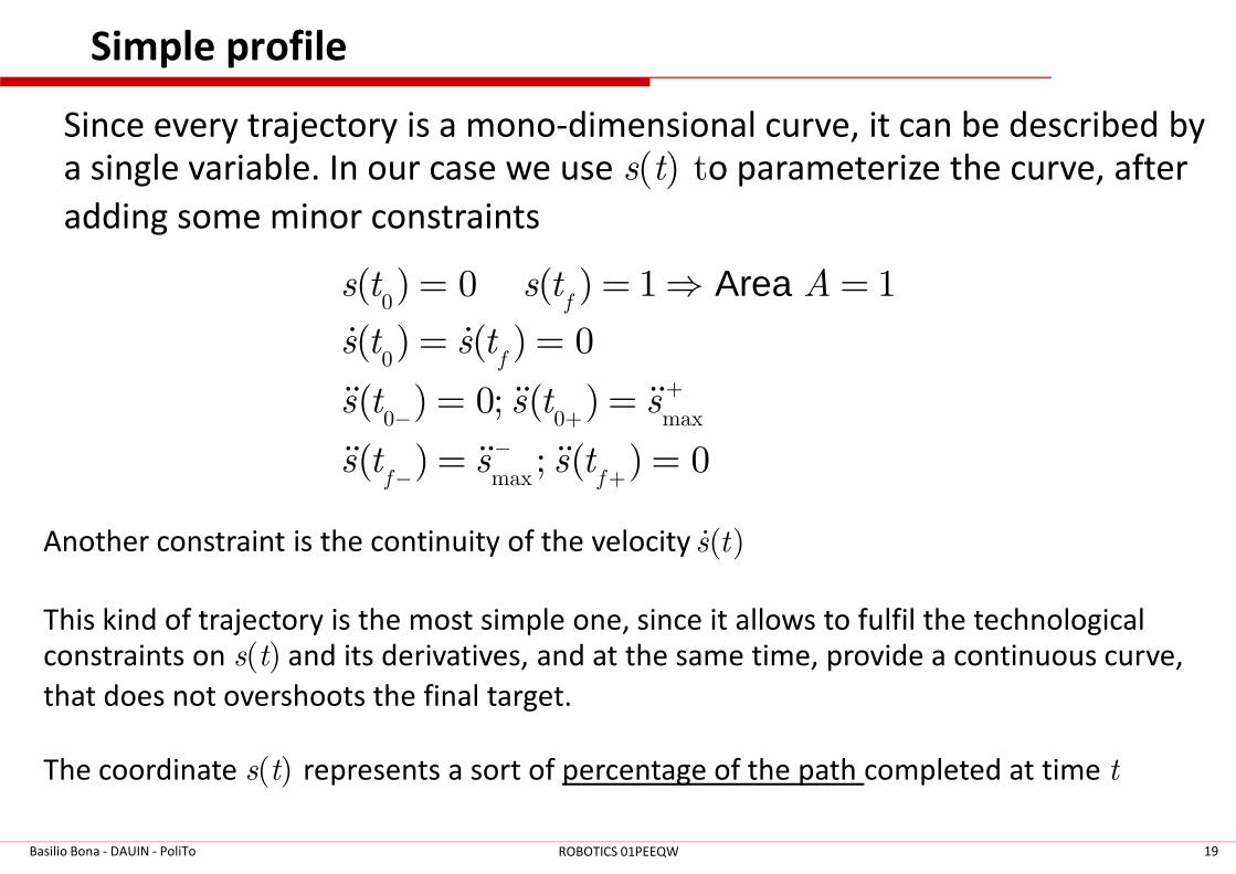
Simple profile
Since every trajectory is a mono-dimensional curve, it can be described by
a single variable. In our case we use s(t) to parameterize the curve, after
adding some minor constraints
Area 0
0
0 0 max
( ) 0 ( ) 1 1
( ) ( ) 0
( ) 0; ( )
f
f
s t s t A
s t s t
s t s t s+− +
−
= = ⇒ =
= =
= =
= =
ɺ ɺ
ɺɺ ɺɺ ɺɺ
ɺɺ ɺɺ ɺɺmax
( ) ; ( ) 0f f
s t s s t−
− += =ɺɺ ɺɺ ɺɺ
Another constraint is the continuity of the velocity
This kind of trajectory is the most simple one, since it allows to fulfil the technological
constraints on s(t) and its derivatives, and at the same time, provide a continuous curve,
that does not overshoots the final target.
The coordinate s(t) represents a sort of percentage of the path completed at time t
( )s tɺ
Basilio Bona - DAUIN - PoliTo 19ROBOTICS 01PEEQW
Continuous ProfileContinuous Profile
Basilio Bona - DAUIN - PoliTo 20ROBOTICS 01PEEQW
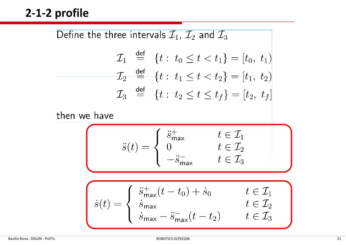
2-1-2 profile
Basilio Bona - DAUIN - PoliTo 21ROBOTICS 01PEEQW
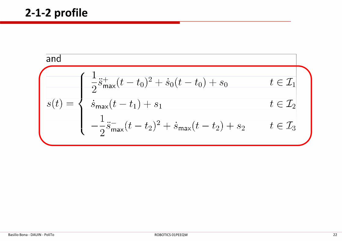
2-1-2 profile
Basilio Bona - DAUIN - PoliTo 22ROBOTICS 01PEEQW
2-1-2 profile
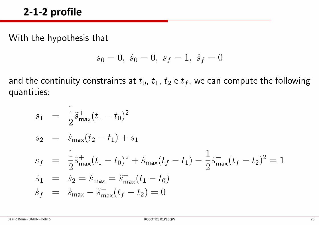
Basilio Bona - DAUIN - PoliTo 23ROBOTICS 01PEEQW
2-1-2 profile
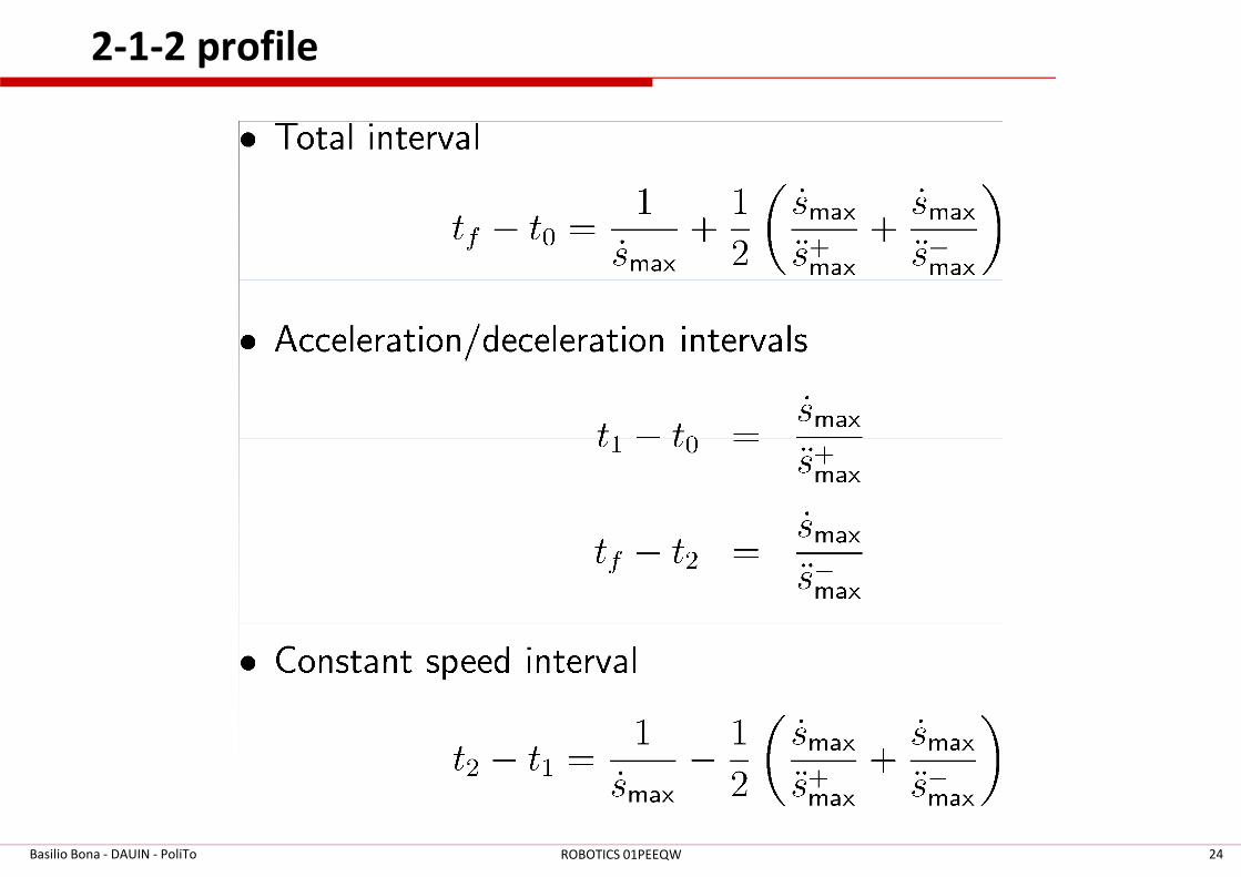
Basilio Bona - DAUIN - PoliTo 24ROBOTICS 01PEEQW
2-1-2 profile
Basilio Bona - DAUIN - PoliTo 25ROBOTICS 01PEEQW
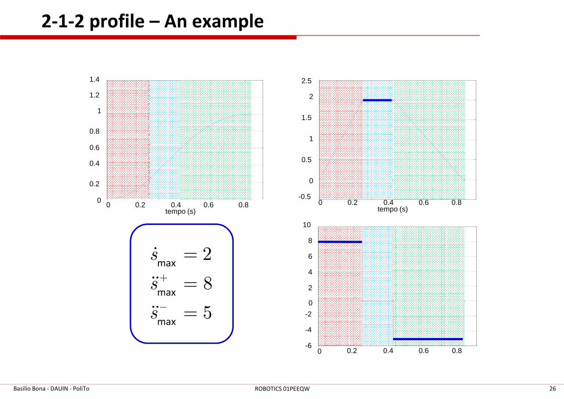
2-1-2 profile – An example
0 0.2 0.4 0.6 0.8-0.5
0
0.5
1
1.5
2
2.5
0
0.2
0.4
0.6
0.8
1
1.2
1.4
Basilio Bona - DAUIN - PoliTo 26ROBOTICS 01PEEQW
0 0.2 0.4 0.6 0.8-0.5
tempo (s)0 0.2 0.4 0.6 0.80
tempo (s)
0 0.2 0.4 0.6 0.8-6
-4
-2
0
2
4
6
8
10
max
max
max
2
8
5
s
s
s
+
−
=
=
=
ɺ
ɺɺ
ɺɺ
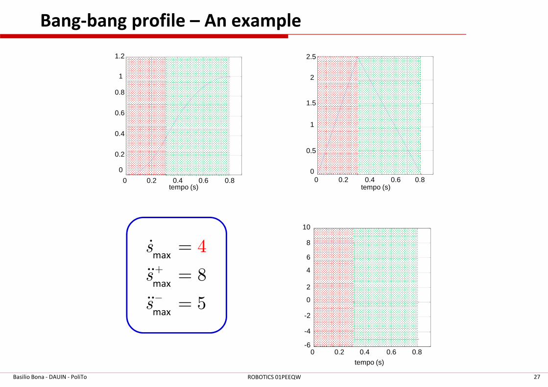
Bang-bang profile – An example
0 0.2 0.4 0.6 0.80
0.5
1
1.5
2
2.5
tempo (s)0 0.2 0.4 0.6 0.8
0
0.2
0.4
0.6
0.8
1
1.2
tempo (s)
Basilio Bona - DAUIN - PoliTo 27ROBOTICS 01PEEQW
max
max
max
8
5
4s
s
s
+
−
=
=
=
ɺ
ɺɺ
ɺɺ
0 0.2 0.4 0.6 0.8-6
-4
-2
0
2
4
6
8
10
tempo (s)

Sampled Data ProfileSampled Data Profile
Basilio Bona - DAUIN - PoliTo 28ROBOTICS 01PEEQW
Discrete Time (sampled data) profile
� Since the manipulator controller is a discrete-time
computer, it is necessary to sample the continuous variable
s(t).
� The sampling interval T is fixed according to the control
specifications, and in modern robots is approximately 1 ms
� A sequence of N samples is obtained as
� The samples are then rounded off to be stored in a fixed
length internal register (it can be a fixed length word or
exponent + mantissa)Basilio Bona - DAUIN - PoliTo 29ROBOTICS 01PEEQW
{ }0 1 1( ) , , , , ,
k Ns t s s s s
−→ … …
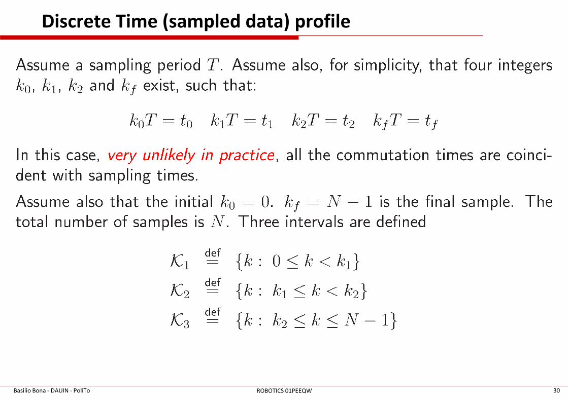
Discrete Time (sampled data) profile
Basilio Bona - DAUIN - PoliTo 30ROBOTICS 01PEEQW
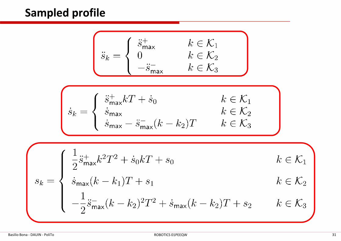
Sampled profile
Basilio Bona - DAUIN - PoliTo 31ROBOTICS 01PEEQW
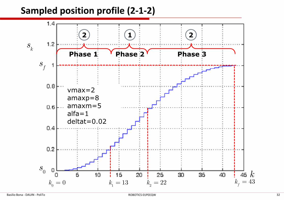
Sampled position profile (2-1-2)
fs
ks
vmax=2amaxp=8
2 21
Phase 1 Phase 2 Phase 3
Basilio Bona - DAUIN - PoliTo 32ROBOTICS 01PEEQW
00k =
0s
113k =
222k = 43
fk =
k
amaxp=8amaxm=5alfa=1deltat=0.02
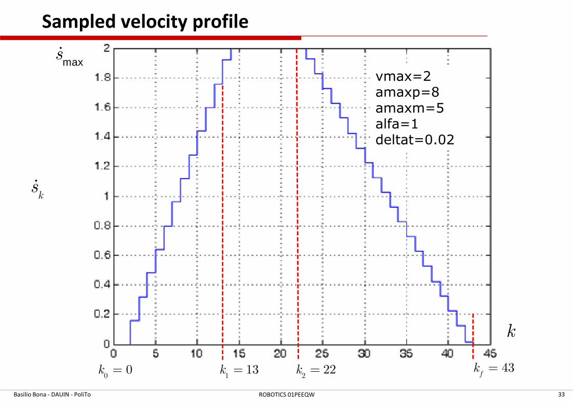
Sampled velocity profile
maxsɺ
ksɺ
vmax=2amaxp=8amaxm=5alfa=1deltat=0.02
Basilio Bona - DAUIN - PoliTo 33ROBOTICS 01PEEQW
k
00k =
113k =
222k = 43
fk =
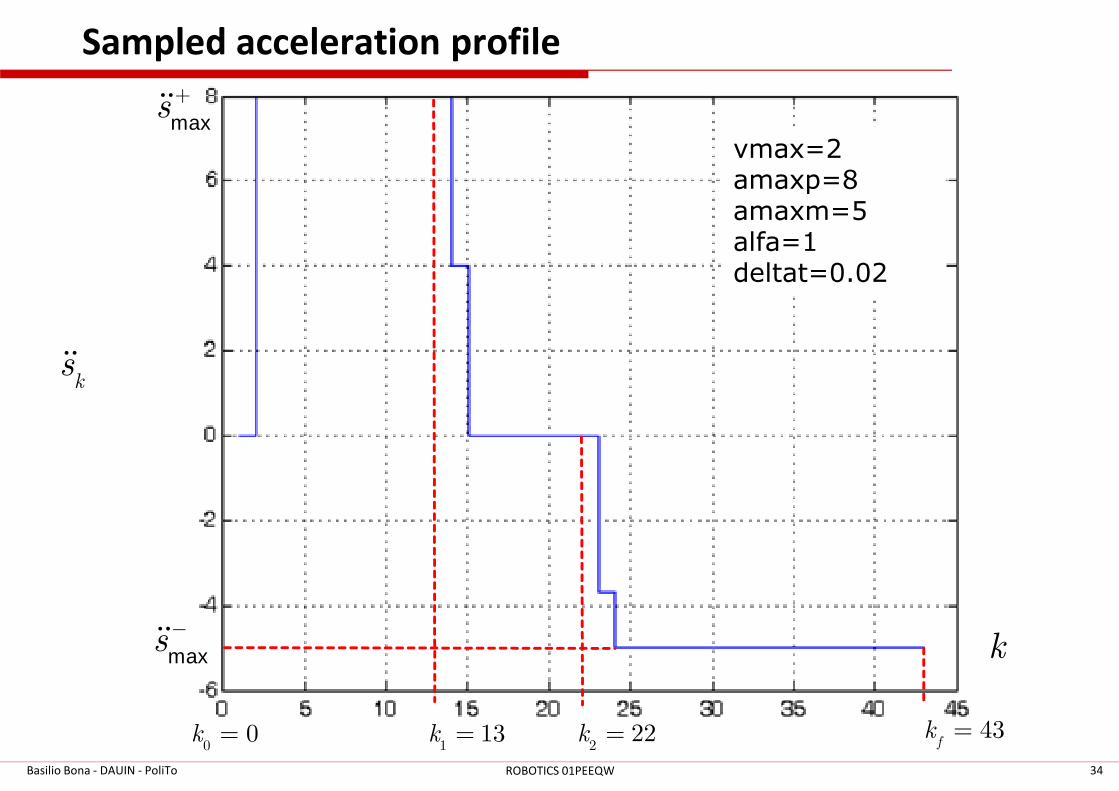
Sampled acceleration profile
maxs+ɺɺ
ksɺɺ
vmax=2amaxp=8amaxm=5alfa=1deltat=0.02
Basilio Bona - DAUIN - PoliTo 34ROBOTICS 01PEEQW
k
00k =
113k =
222k = 43
fk =
maxs−ɺɺ
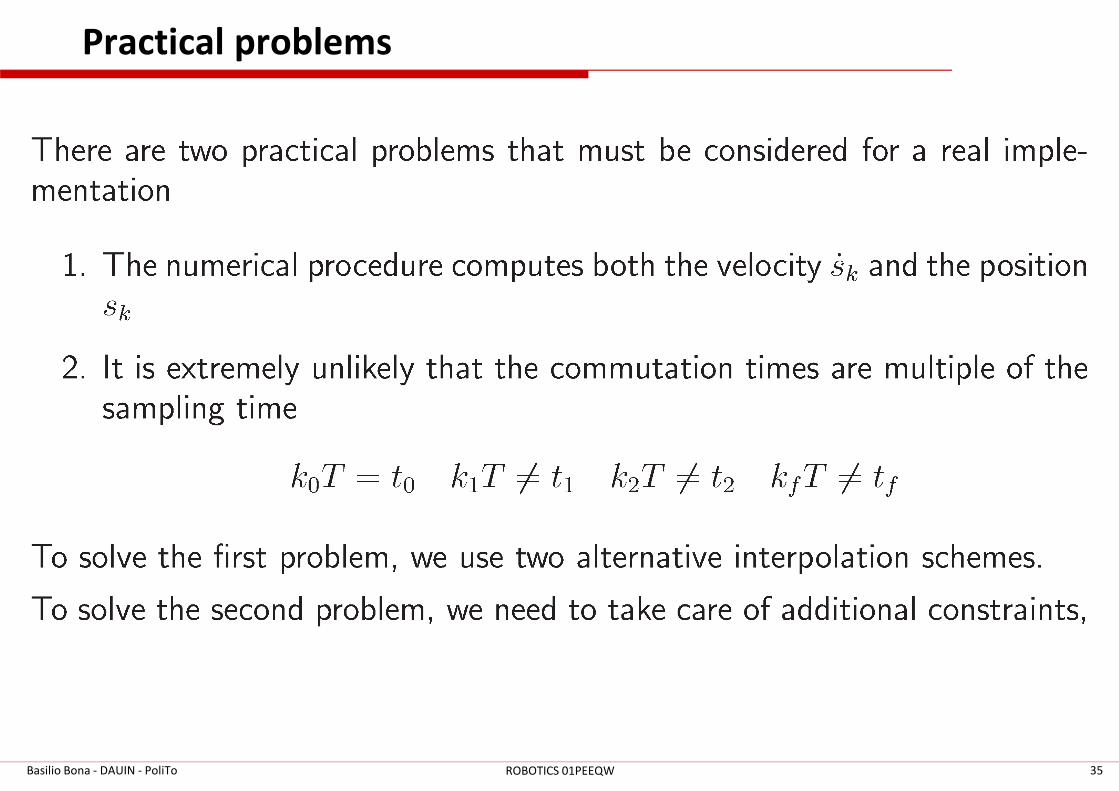
Practical problems
Basilio Bona - DAUIN - PoliTo 35ROBOTICS 01PEEQW
Interpolation schemes
Basilio Bona - DAUIN - PoliTo 36ROBOTICS 01PEEQW
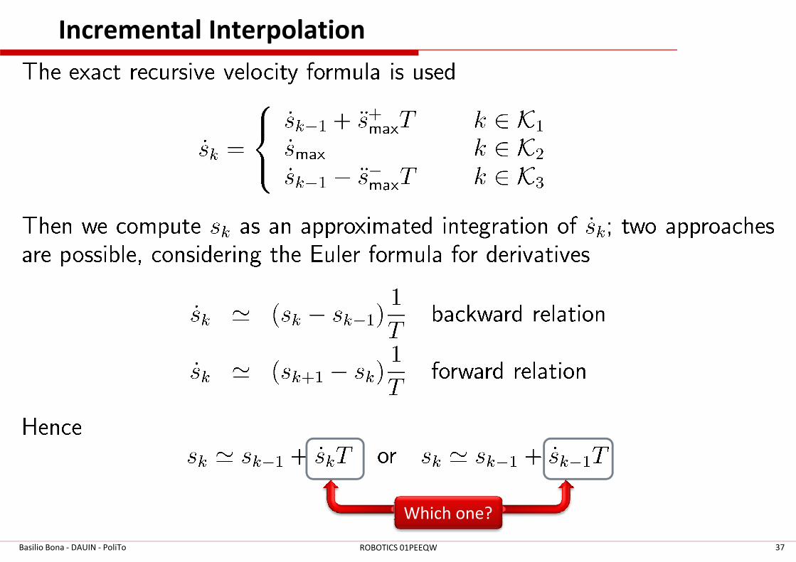
Incremental Interpolation
Which one?
Basilio Bona - DAUIN - PoliTo 37ROBOTICS 01PEEQW
Incremental Interpolation
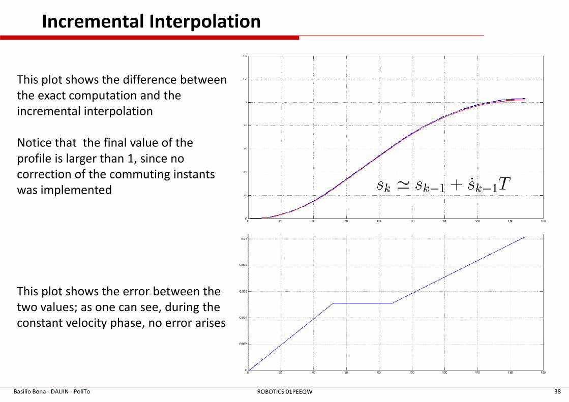
This plot shows the difference between
the exact computation and the
incremental interpolation
Notice that the final value of the
profile is larger than 1, since no
correction of the commuting instants
was implemented
Basilio Bona - DAUIN - PoliTo 38ROBOTICS 01PEEQW
This plot shows the error between the
two values; as one can see, during the
constant velocity phase, no error arises
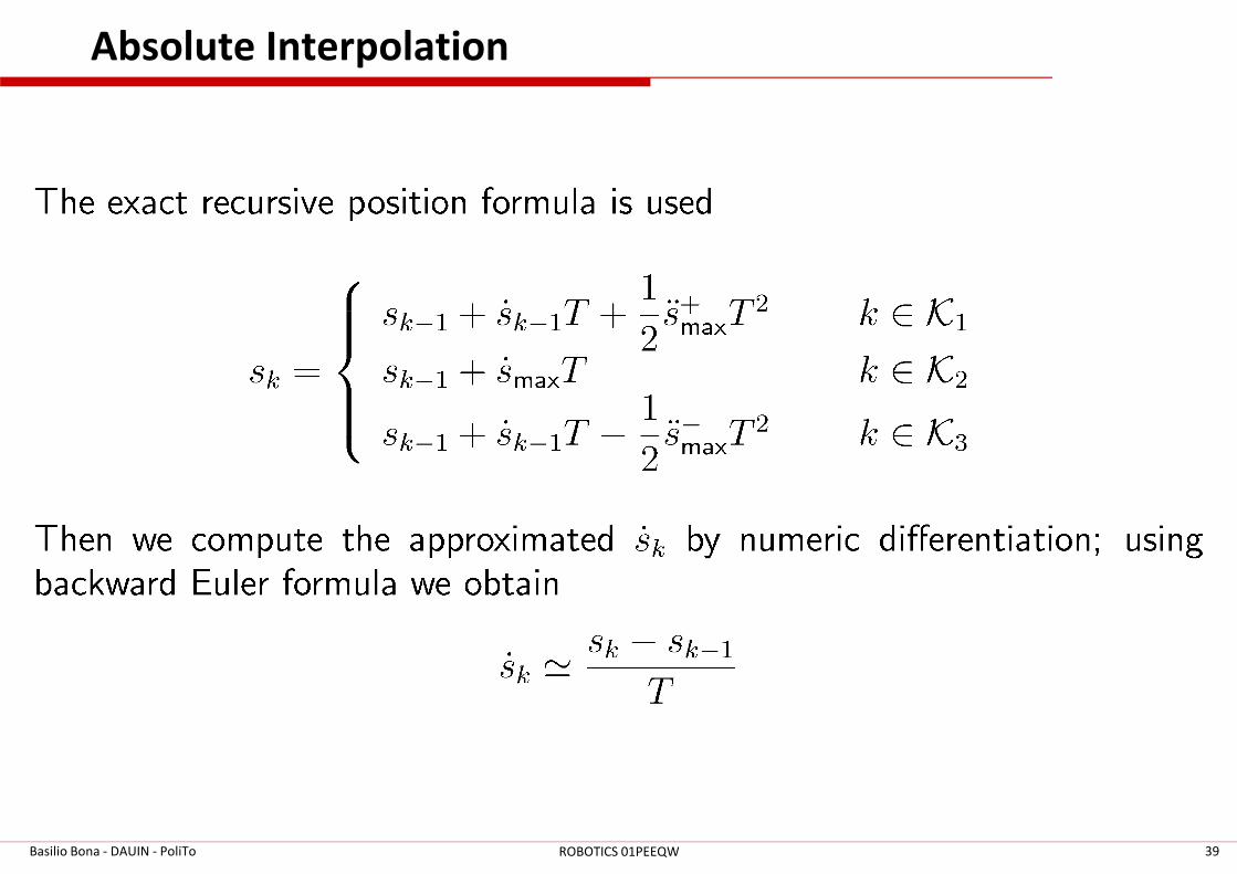
Absolute Interpolation
Basilio Bona - DAUIN - PoliTo 39ROBOTICS 01PEEQW
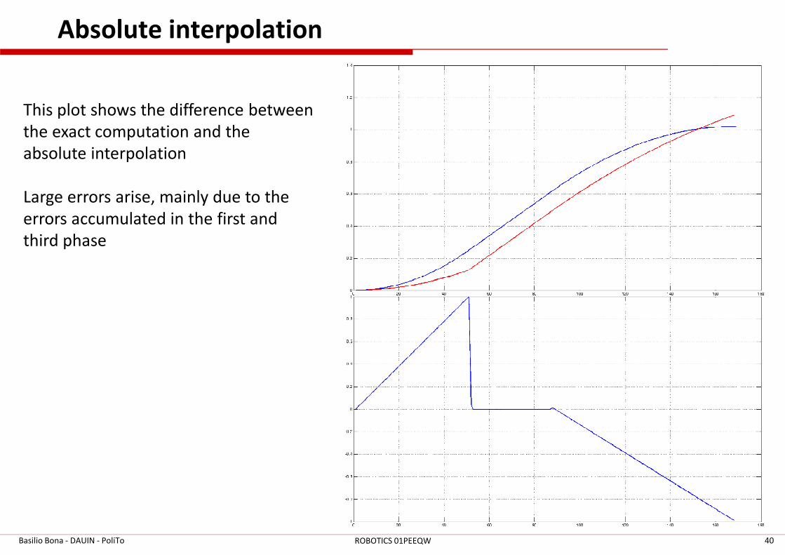
Absolute interpolation
This plot shows the difference between
the exact computation and the
absolute interpolation
Large errors arise, mainly due to the
errors accumulated in the first and
third phase
Basilio Bona - DAUIN - PoliTo 40ROBOTICS 01PEEQW
Approximation of commutation instants
� Since the commutation times are rarely an exact multiple
of the sampling period, it is necessary to compute the
profile so that the profile constraints are never violated
� We proceed as follows
� We compute the new profile samples recursively
� The transition between the acceleration phase and the
constant speed phase is computed so that the maximal constant speed phase is computed so that the maximal
velocity is not exceeded
� The transition between constant speed phase and the
deceleration phase is computed so that
a) The maximal deceleration is not exceeded
b) There is sufficient time intervals to decelerate and reach the
zero final speed without violating a)
c) The final zero velocity must be reached “uniformly” from above
Basilio Bona - DAUIN - PoliTo 41ROBOTICS 01PEEQW
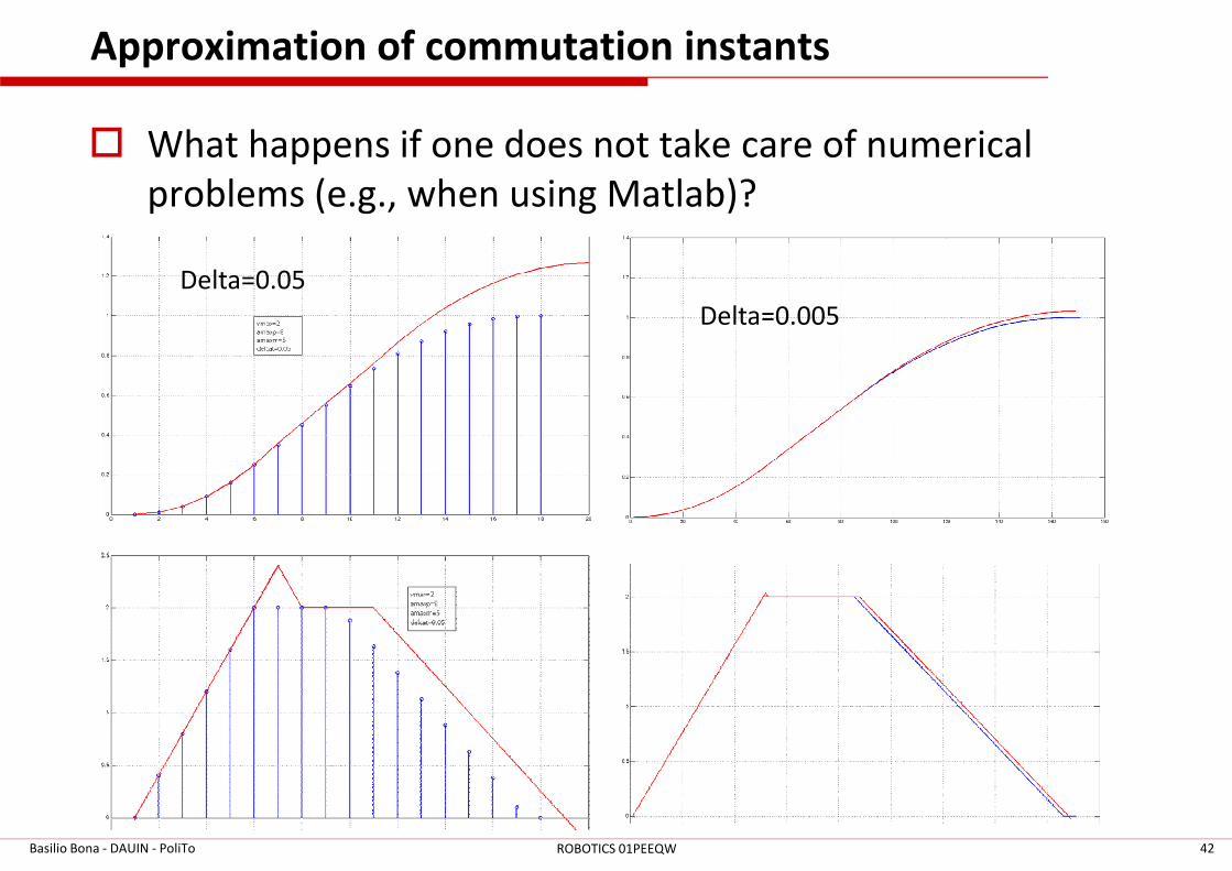
Approximation of commutation instants
� What happens if one does not take care of numerical
problems (e.g., when using Matlab)?
Delta=0.005
Delta=0.05
Basilio Bona - DAUIN - PoliTo 42ROBOTICS 01PEEQW
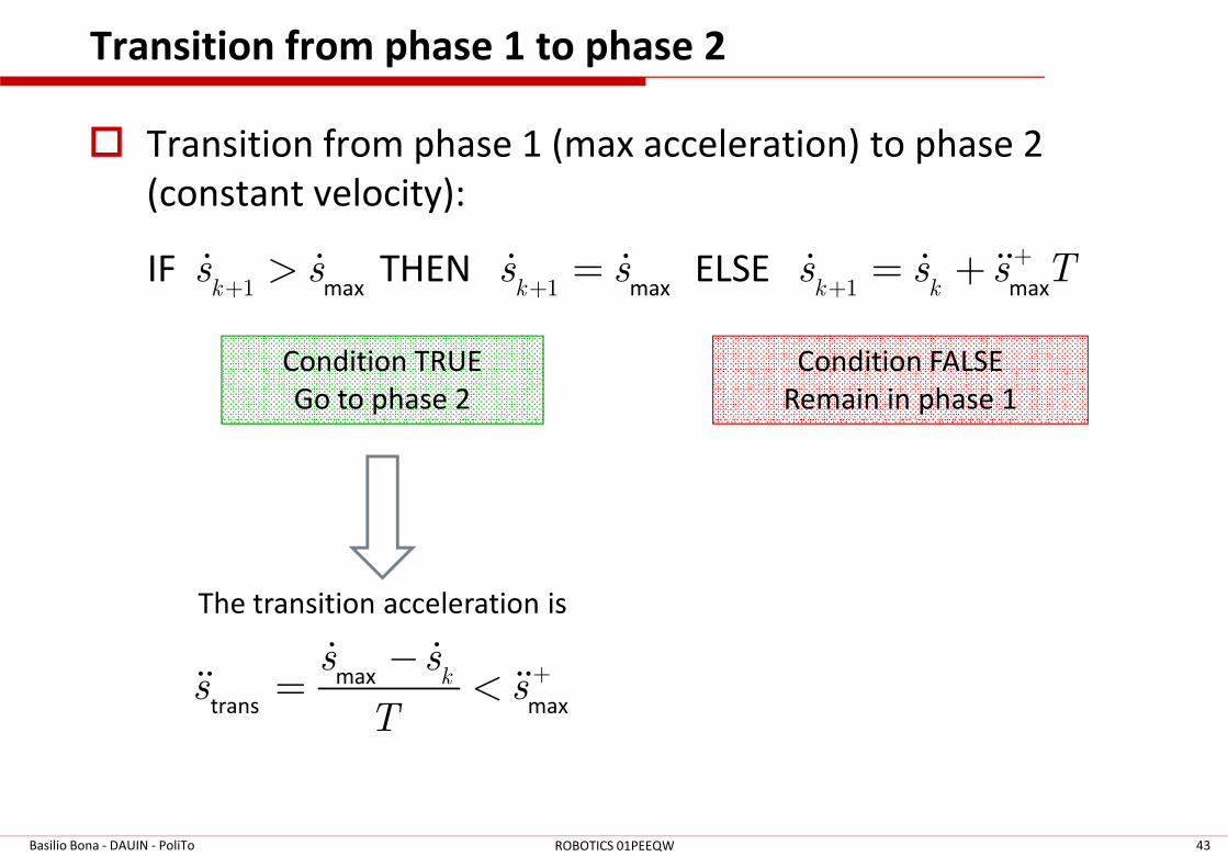
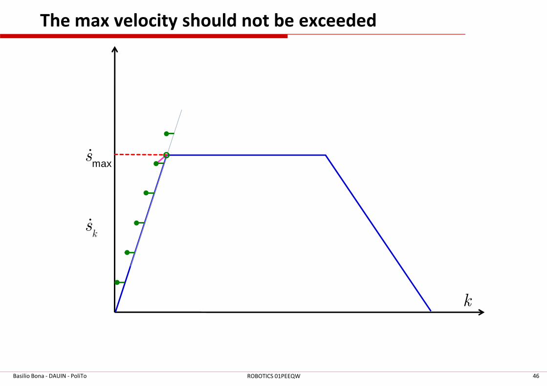
Transition from phase 1 to phase 2
� Transition from phase 1 (max acceleration) to phase 2
(constant velocity):
�
max max maxIF THEN ELSE
1 1 1k k k ks s s s s s s T++ + +> = = +ɺ ɺ ɺ ɺ ɺ ɺ ɺɺ
Condition TRUE
Go to phase 2
Condition FALSE
Remain in phase 1
Basilio Bona - DAUIN - PoliTo 43ROBOTICS 01PEEQW
The transition acceleration is
ks s
s sT
+−= <ɺ ɺ
ɺɺ ɺɺmax
trans max
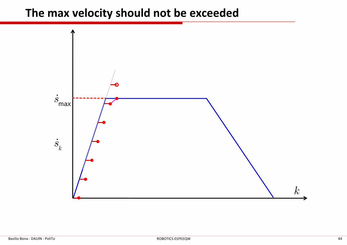
The max velocity should not be exceeded
maxsɺ
Basilio Bona - DAUIN - PoliTo 44ROBOTICS 01PEEQW
ksɺ
k
Basilio Bona - DAUIN - PoliTo 45ROBOTICS 01PEEQW
The max velocity should not be exceeded
maxsɺ
Basilio Bona - DAUIN - PoliTo 46ROBOTICS 01PEEQW
ksɺ
k
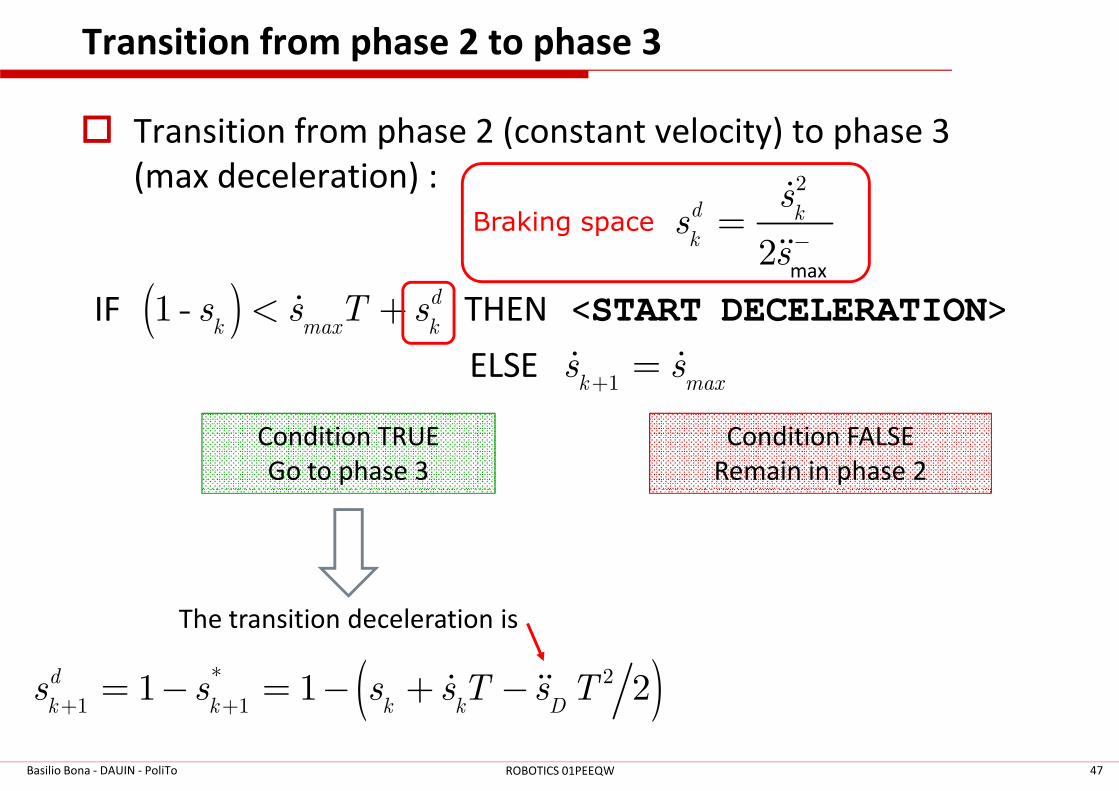
Transition from phase 2 to phase 3
� Transition from phase 2 (constant velocity) to phase 3
(max deceleration) :
�
( )IF THEN < >
ELSE 1
1 - d
k max k
k max
s s T s
s s+
< +
=
ɺ
ɺ ɺ
START DECELERATION
Braking space
max
2
2
d k
k
ss
s−=ɺ
ɺɺ
Basilio Bona - DAUIN - PoliTo 47ROBOTICS 01PEEQW
Condition TRUE
Go to phase 3
Condition FALSE
Remain in phase 2
The transition deceleration is
( )* 2
1 11 1 2d
k k k k Ds s s s T s T+ += − = − + −ɺ ɺɺ
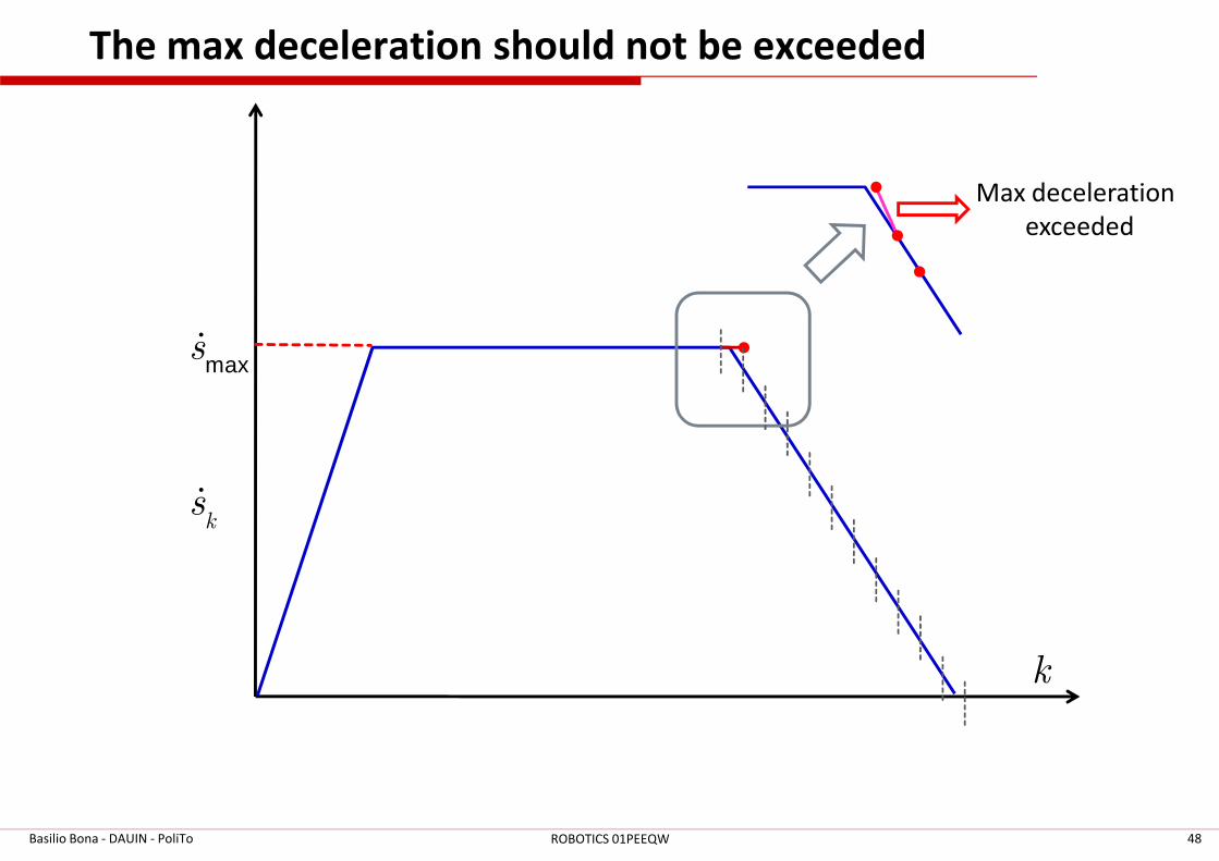
The max deceleration should not be exceeded
maxsɺ
Max deceleration
exceeded
Basilio Bona - DAUIN - PoliTo 48ROBOTICS 01PEEQW
ksɺ
k
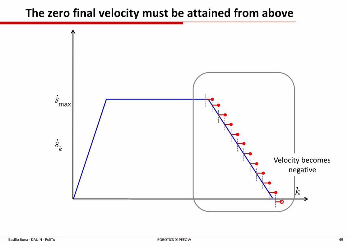
The zero final velocity must be attained from above
maxsɺ
Basilio Bona - DAUIN - PoliTo 49ROBOTICS 01PEEQW
ksɺ
k
Velocity becomes
negative
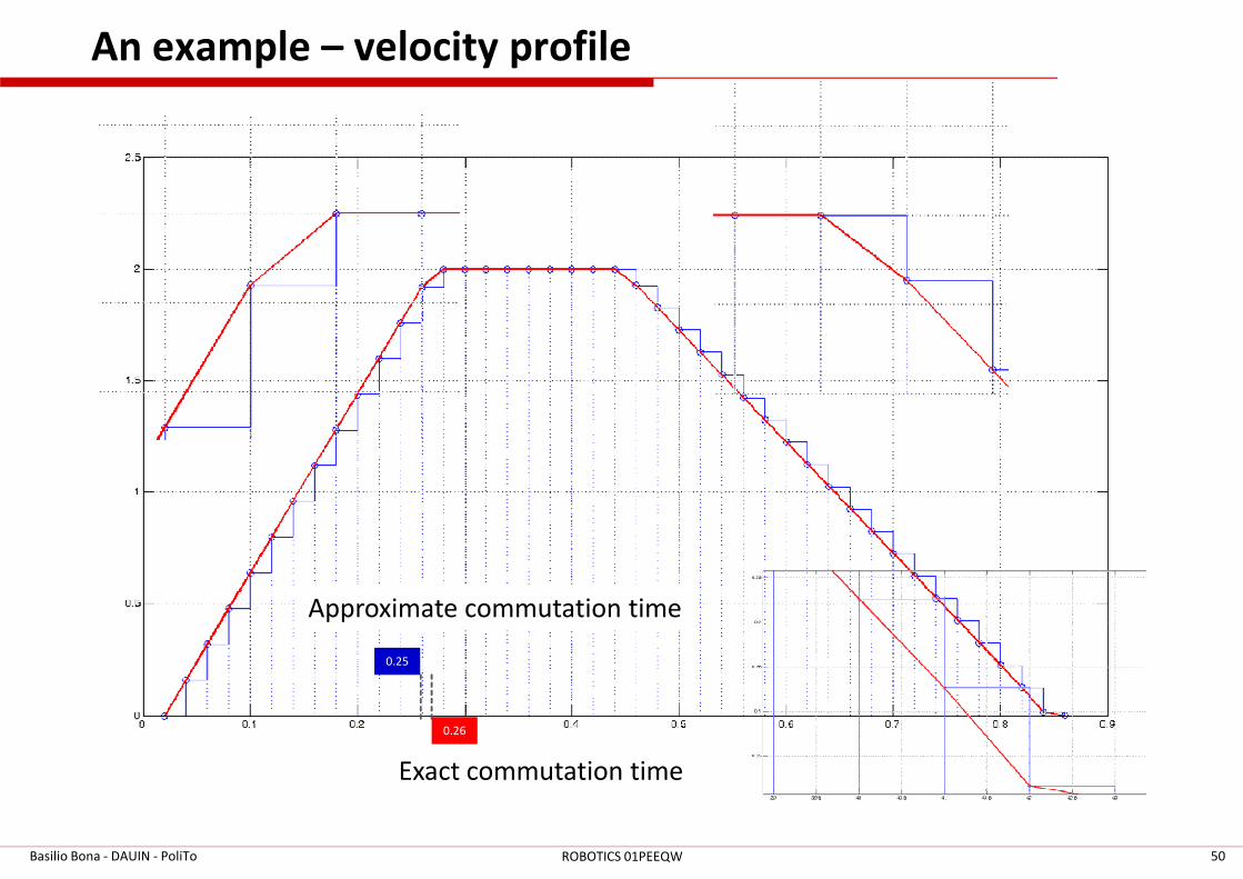
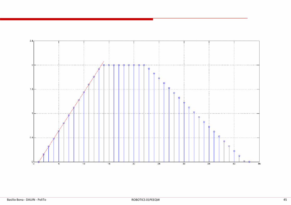
An example – velocity profile
Basilio Bona - DAUIN - PoliTo 50ROBOTICS 01PEEQW
0.26
0.25
Exact commutation time
Approximate commutation time
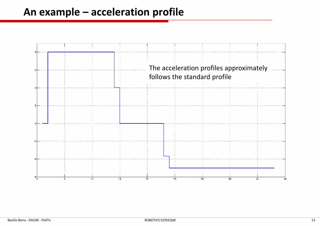
An example – acceleration profile
The acceleration profiles approximately
follows the standard profile
Basilio Bona - DAUIN - PoliTo 51ROBOTICS 01PEEQW
Joint trajectory planning
Basilio Bona - DAUIN - PoliTo 52ROBOTICS 01PEEQW
Joint point-to-point trajectory planning
Point-to-point joint trajectory
Basilio Bona - DAUIN - PoliTo 53ROBOTICS 01PEEQW
Point-to-point joint trajectory
Continuous time
Discrete time
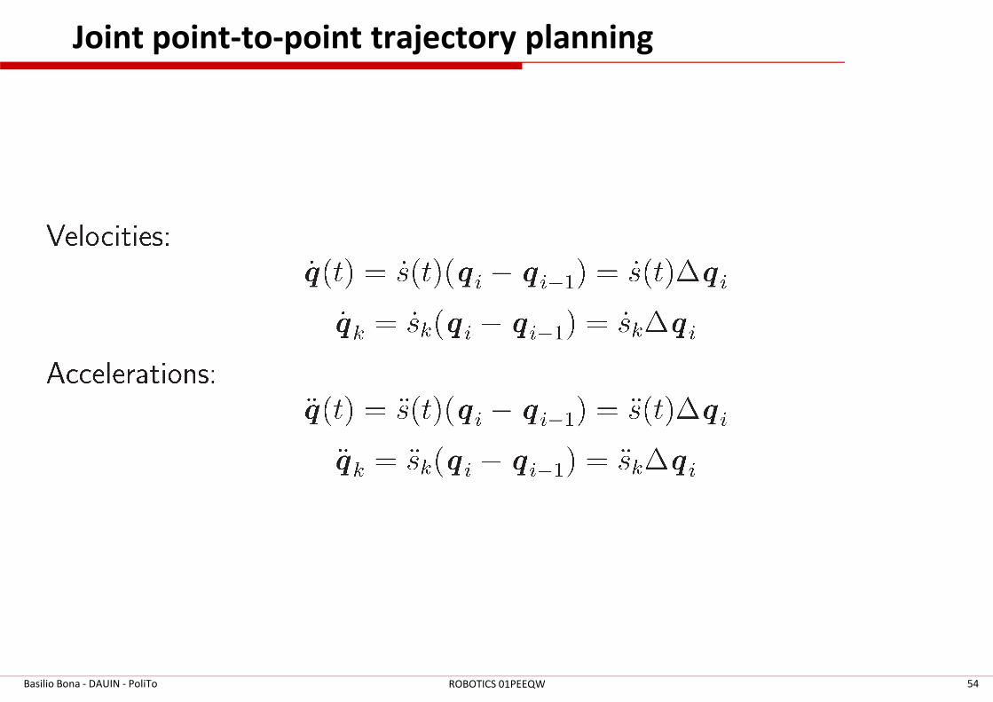
Joint point-to-point trajectory planning
Basilio Bona - DAUIN - PoliTo 54ROBOTICS 01PEEQW
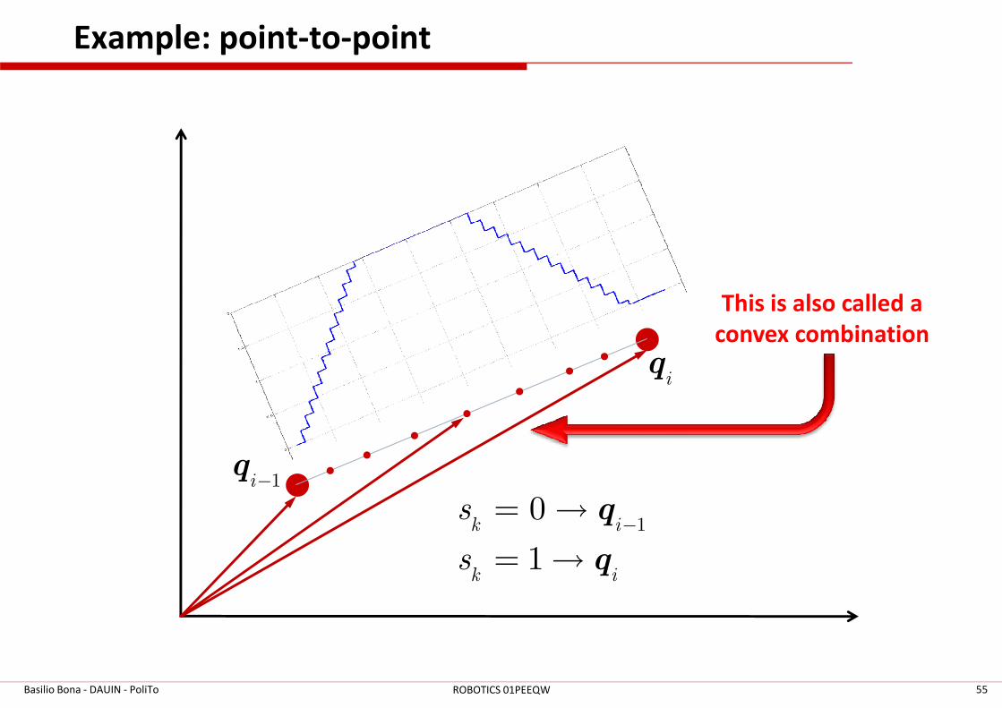
Example: point-to-point
q
This is also called a
convex combination
Basilio Bona - DAUIN - PoliTo 55ROBOTICS 01PEEQW
iq
1i−q
10
1k i
k i
s
s
−= →
= →
q
q
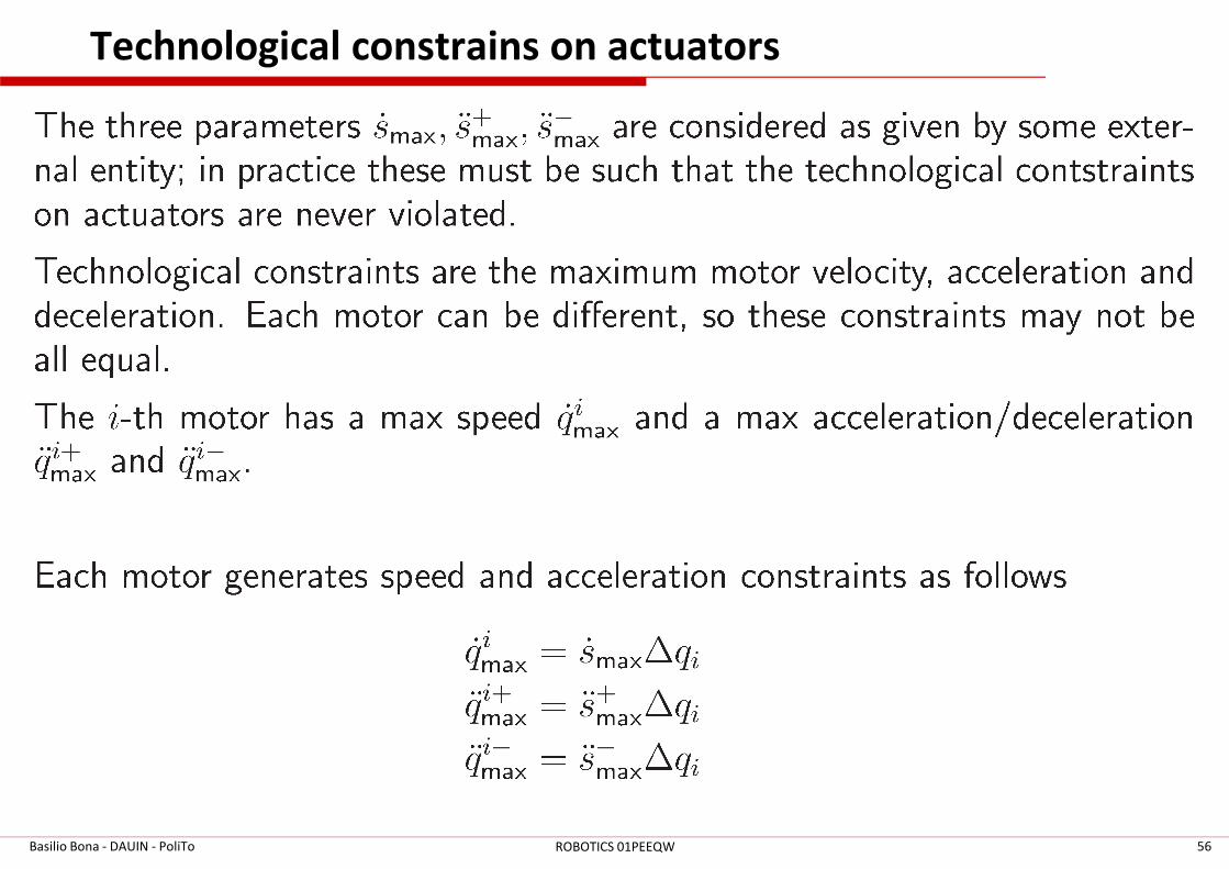
Technological constrains on actuators
Basilio Bona - DAUIN - PoliTo 56ROBOTICS 01PEEQW
Technological constrains on actuators
Basilio Bona - DAUIN - PoliTo 57ROBOTICS 01PEEQW
Conclusions
� Path planning is a very important issue in robotics
� The geometrical path (and its time law) provides the
reference data necessary for any control implementation
� A real path planning algorithm must work in discrete time,
(often in real-time) since robot acts on a sampled data (often in real-time) since robot acts on a sampled data
control system
� Path planning may be defined in joint space or task space
� Task space planning requires the computation of inverse
kinematic functions (beware of singularities)
Basilio Bona - DAUIN - PoliTo 58ROBOTICS 01PEEQW