1

Giorgio Grisetti, Cyrill Stachniss,

Kai Arras, Maren Bennewitz, Wolfram Burgard

Robotics 2A Compact Course on Linear Algebra

2

Vectors

� Arrays of numbers

� They represent a point in a ndimensional space

3

Vectors: Scalar Product

� Scalar-Vector Product

� Changes the length of the vector, but not its direction

4

Vectors: Sum

� Sum of vectors (is commutative)

� Can be visualized as “chaining” the vectors.

5

Vectors: Dot Product

� Inner product of vectors (is a scalar)

� If one of the two vectors has , the inner product returns the length of the projection of along the direction of

•If the two vectors are orthogonal

6

� A vector is linearly dependent from

if

� In other words if can be obtained by summing up the properly scaled.

� If do not exist such that then is independent from

Vectors: Linear (In)Dependence

7

� A vector is linearly dependent from

if

� In other words if can be obtained by summing up the properly scaled.

� If do not exist such that then is independent from

Vectors: Linear (In)Dependence

8

Matrices

� A matrix is written as a table of values

� Can be used in many ways:

9

Matrices as Collections of Vectors

� Column vectors

10

Matrices as Collections of Vectors

� Row Vectors

11

Matrices Operations

� Sum (commutative, associative)

� Product (not commutative)

� Inversion (square, full rank)

� Transposition

� Multiplication by a scalar

� Multiplication by a vector

12

Matrix Vector Product

� The i component of is the dot product .

� The vector is linearly dependent from with coefficients .

13

Matrix Vector Product

� If the column vectors represent a reference system, the product computes the global transformation of the vector according to

14

Matrix Vector Product

� Each can be seen as a linear mixing coefficient that tells how contributes to .

� Example: Jacobian of a multi-dimensional function

15

Matrix Matrix Product

� Can be defined through

� the dot product of row and column vectors

� the linear combination of the columns of Ascaled by the coefficients of the columns of B.

16

Matrix Matrix Product

� If we consider the second interpretation we see that the columns of C are the projections of the columns of B through A.

� All the interpretations made for the matrix vector product hold.

17

Linear Systems

� Interpretations:� Find the coordinates x in the reference system of A such that b is the result of the transformation of Ax.

� Many efficient solvers� Conjugate gradients

� Sparse Cholesky Decomposition (if SPD)

� …

� The system may be over or under constrained.

� One can obtain a reduced system (A’ b’) by considering the matrix (A b) and suppressing all the rows which are linearly dependent.

18

Linear Systems

� The system is over-constrained if the number of linearly independent columns (or rows) of A’ is greater than the dimension of b’.

� An over-constrained system does not admit a solution, however one may find a minimum norm solution by pseudo inversion

19

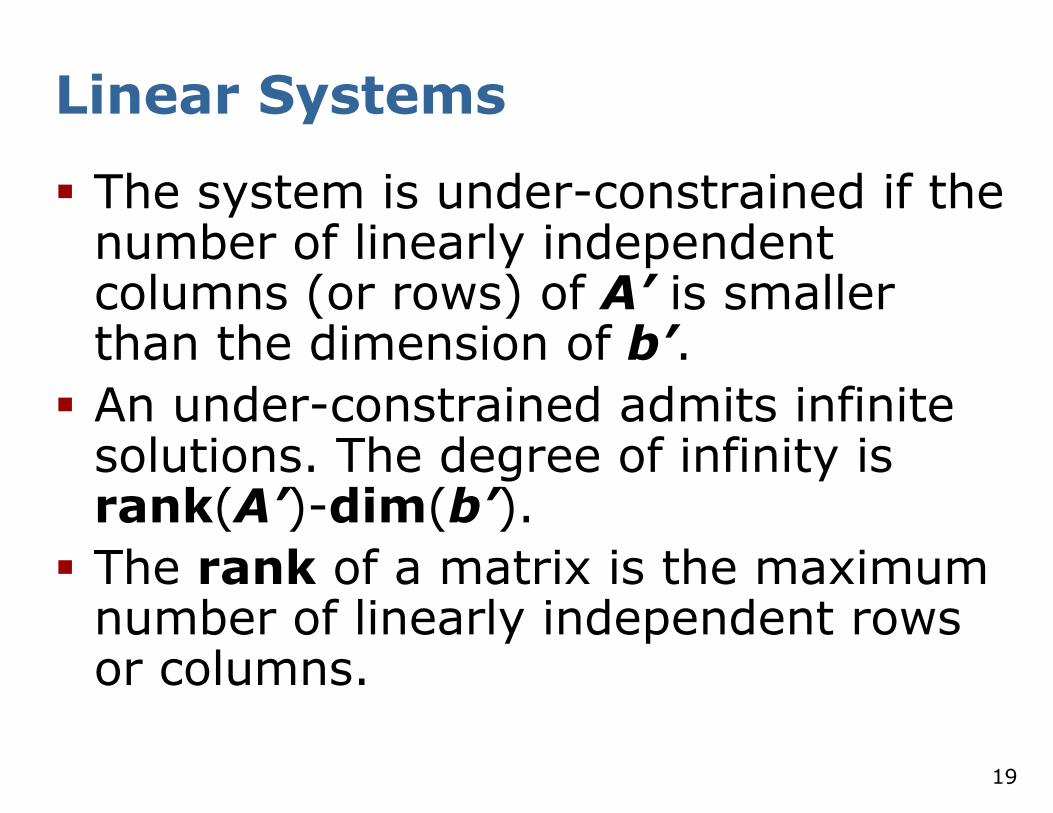
Linear Systems

� The system is under-constrained if the number of linearly independent columns (or rows) of A’ is smaller than the dimension of b’.

� An under-constrained admits infinite solutions. The degree of infinity is rank(A’)-dim(b’).

� The rank of a matrix is the maximum number of linearly independent rows or columns.

20

Matrix Inversion

� If A is a square matrix of full rank, then there is a unique matrix B=A-1 such that the above equation holds.

� The ith row of A is and the jth column of A-1

are:� orthogonal, if i=j� their scalar product is 1, otherwise.

� The ith column of A-1 can be found by solving the following system:

This is the ith column of the identity matrix

21

� Only defined for square matrices

� Sum of the elements on the main diagonal, that is

� It is a linear operator with the following properties

� Additivity:

� Homogeneity:

� Pairwise commutative:

� Trace is similarity invariant

� Trace is transpose invariant

Trace

22

� Maximum number of linearly independent rows (columns)

� Dimension of the image of the transformation

� When is we have

� and the equality holds iff is the null matrix

�

� is injective iff

� is surjective iff

� if , is bijective and is invertible iff

� Computation of the rank is done by

� Perform Gaussian elimination on the matrix

� Count the number of non-zero rows

Rank

23

� Only defined for square matrices

� Remember? if and only if

� For matrices:

Let and , then

� For matrices:

Determinant

24

� For general matrices?

Let be the submatrix obtained from by deleting the i-th row and the j-th column

Rewrite determinant for matrices:

Determinant

25

� For general matrices?

Let be the (i,j)-cofactor, then

This is called the cofactor expansion across the first row.

Determinant

26

� Problem: Take a 25 x 25 matrix (which is considered small).

The cofactor expansion method requires n! multiplications.

For n = 25, this is 1.5 x 10^25 multiplications for which a

today supercomputer would take 500,000 years.

� There are much faster methods, namely using Gauss

elimination to bring the matrix into triangular form

Then:

Because for triangular matrices (with being invertible),

the determinant is the product of diagonal elements

Determinant

27

Determinant: Properties

� Row operations ( still a square matrix)

� If results from by interchanging two rows,

then

� If results from by multiplying one row with a number ,

then

� If results from by adding a multiple of one row to another

row, then

� Transpose:

� Multiplication:

� Does not apply to addition!

28

Determinant: Applications

� Find the inverse using Cramer’s rule

with being the adjugate of

� Compute Eigenvalues

Solve the characteristic polynomial

� Area and Volume:

( is i-th row)

29

� A matrix is orthogonal iff its column (row) vectors represent an orthonormal basis

� As linear transformation, it is norm preserving, and acts as an isometry in Euclidean space (rotation, reflection)

� Some properties:� The transpose is the inverse

� Determinant has unity norm (§ 1)

Orthogonal matrix

30

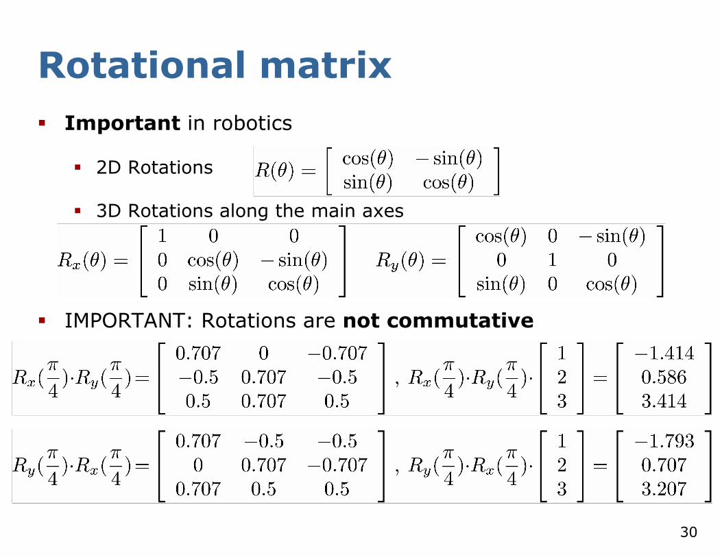
� Important in robotics

� 2D Rotations

� 3D Rotations along the main axes

� IMPORTANT: Rotations are not commutative

Rotational matrix

31

Matrices as Affine Transformations

� A general and easy way to describe a 3D transformation is via matrices.

� Homogeneous behavior in 2D and 3D

� Takes naturally into account the non-commutativity of the transformations

Rotation Matrix

Translation Vector

32

Combining Transformations

� A simple interpretation: chaining of transformations (represented as homogeneous matrices)� Matrix A represents the pose of a robot in the space� Matrix B represents the position of a sensor on the robot� The sensor perceives an object at a given location p, in its own

frame [the sensor has no clue on where it is in the world]� Where is the object in the global frame?

p

33

Combining Transformations

� A simple interpretation: chaining of transformations (represented ad homogeneous matrices)� Matrix A represents the pose of a robot in the space� Matrix B represents the position of a sensor on the robot� The sensor perceives an object at a given location p, in its own

frame [the sensor has no clue on where it is in the world]� Where is the object in the global frame?

p

B

Bp gives me the pose of the object wrt the robot

34

Combining Transformations

� A simple interpretation: chaining of transformations (represented ad homogeneous matrices)� Matrix A represents the pose of a robot in the space� Matrix B represents the position of a sensor on the robot� The sensor perceives an object at a given location p, in its own

frame [the sensor has no clue on where it is in the world]� Where is the object in the global frame?

p

B

Bp gives me the pose of the object wrt the robot

ABp gives me the pose of the object wrt the world

A

35

� A matrix is symmetric if , e.g.

� A matrix is anti-symmetric if , e.g.

� Every symmetric matrix:� can be diagonalizable , where is a diagonal

matrix of eigenvalues and is an orthogonal matrix whose columns are the eigenvectors of

� define a quadratic form

Symmetric matrix

36

� The analogous of positive number

� Definition

�

� Examples

�

�

Positive definite matrix

37

� Properties

� Invertible, with positive definite inverse

� All eigenvalues > 0

� Trace is > 0

� For any spd , are positive definite

� Cholesky decomposition

� Partial ordering: iff

� If , we have

� If , then

�

�

Positive definite matrix

38

Jacobian Matrix

• It’s a non-square matrix in general

• Suppose you have a vector-valued function

• Let the gradient operator be the vector of (first-order)

partial derivatives

Then, the Jacobian matrix is defined as

39

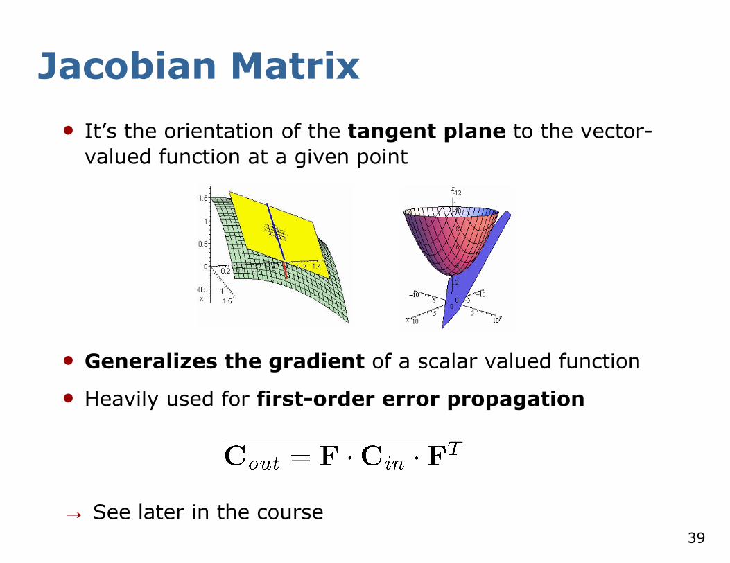
• It’s the orientation of the tangent plane to the vector-

valued function at a given point

• Generalizes the gradient of a scalar valued function

• Heavily used for first-order error propagation

→ See later in the course

Jacobian Matrix

40

Quadratic Forms

� Many important functions can be locally approximated with a quadratic form.

� Often one is interested in finding the minimum (or maximum) of a quadratic form.

41

Quadratic Forms

� How can we use the matrix properties to quickly compute a solution to this minimization problem?

� At the minimum we have

� By using the definition of matrix product we can compute f’

42

Quadratic Forms

� The minimum of is where its derivative is set to 0

� Thus we can solve the system

� If the matrix is symmetric, the system becomes