Robot Spatial Perception Stereoscopic Vision 3D...

Robot Spatial Perception by Stereoscopic Visionand 3D Evidence Grids

Hans P. Moravec

CMU-RI-TR-96-34

The Robotics InstituteCarnegie Mellon University

Pittsburgh, Pennsylvania 15213

September 1996

1996 Carnegie Mellon University

Portions of this research were sponsored by the Office of Naval Researchunder contract number N0094-93-1-0765, by Daimler Benz Research, Berlin,

by Thinking Machines Corp., and by the CMU Robotics Institute

Acknowledgments:This work was done while the author was on a six month sabbatical visit. Thanks to my hosts FriederLohnert, Dimitris Georgianis, Volker Hansen and the other members of Daimler Benz Research, Berlin,who provided the encouragement and means to complete this work. Special thanks go to Ralph Sasse forseveral times volunteering critical help, taking time from his own consuming research. Thanks also to myCMU support network, especially Martin Martin, Mike Blackwell and Kevin Dowling. A major compo-nent of the program described here, the evidence ray thrower, was written during my 1992 sabbaticalyear at Thinking Machines Corp. in Cambridge, Massachusetts - many thanks for that opportunity. Longterm support for this research was provided since 1982 by the US Office of Naval Research underN00014-93-1-0765 and previous contracts. The impetus for the evidence grid idea came from a researchcontract from Denning Mobile Robotics Inc. in 1983. Final thanks go to Christopher Priem for so care-fully studying my program, and generating the large data set whose images are found in the report’sappendix.

Introduction 1

Robot Spatial Perception by Stereoscopic Visionand 3D Evidence Grids

Abstract

Very encouraging results have been obtained from a new program that derives a dense three-dimensionalevidence grid representation of a robot’s surroundings from wide-angle stereoscopic images. The pro-gram adds several spatial rays of evidence to a grid for each of about 2,500 local image features chosenper stereo pair. It was used to construct a 256x256x64 grid, representing 6 by 6 by 2 meters, from a hand-collected test set of twenty stereo image pairs of an office scene. Fifty nine stereo pairs of an 8 by 8 meterlaboratory were also processed. The positive (probably occupied) cells of the grids, viewed in perspec-tive, resemble dollhouse scenes. Details as small as the curvature of chair armrests are discernible. Theprocessing time, on a 100 MIPS Sparc 20, is less than five seconds per stereo pair, and total memory isunder 16 megabytes. The results seem abundantly adequate for very reliable navigation of freely roamingmobile robots, and plausibly adequate for shape identification of objects bigger than 10 centimeters. Theprogram is a first proof of concept, and awaits optimizations, enhancements, variations, extensions andapplications.

1 Introduction

This report describes a new program that transforms stereoscopic images, as could be obtained froma camera-equipped roving robot, into dense three-dimensional maps of the robot’s immediate sur-roundings. The program generates 100 to 1,000 times as much good map data as previous systemsrelying on 2D or sparse 3D representations, suggesting that the statistical reliability of navigationprograms using on it should be very high. The program was tested with 20 stereo image pairs of anoffice, and a second data set of 59 stereo pairs of a larger laboratory. The resulting 3D maps show ob-ject details to a scale of about 10 cm. By using higher resolution grids, features of a few centimeterscan be resolved.

Before mapping, the stereo camera fixture is calibrated. The fixture is leveled, and positioned, withreasonable accuracy, perpendicularly a known distance in front of a screen patterned with a precisesquare array of about 400 black spots on a white background. A program, designed to deal with thefish-eye distortion of wide angle lenses, finds the spots in the cameras’ digitized images, and con-structs a rectification function for each camera that corrects for the distortion and small mounting mis-alignments. In use, the rectification functions are compiled into image-sized lookup tables, whichgeometrically transform raw camera images so they appear to have come from a specified ideal op-tical geometry.

During mapping, a sequence of stereo image pairs is processed. The results accumulate in a three-dimensional array called an evidence grid, whose cells represent regions of space. Each grid cell accu-mulates evidence, positive and negative, that its region is occupied. The grid cells are initialized tozero, indicating no evidence for or against the cell being occupied. After sufficient data has accumu-lated, blocks of negative cells indicate free space, while positive cells define objects. The program’scomputationally efficient additive “weight of evidence” metric can be interpreted in probability the-

ory as Bayesian combination using a “log-odds” representation of probability.p1 p–------------log

2 Robot Spatial Perception by Stereoscopic Vision and 3D Evidence Grids

Processing of each stereo pair begins with image rectification. An interest operator then selects about2,500 local features in the two images, each chosen to be a good candidate for locating in the otherimage of the pair. For each feature, a correlator scans the possible corresponding locations in the otherimage, producing a curve of goodness of match. The peaks in this curve each correspond to a possibledistance for the feature. For each of the possibilities, the program throws two rays of evidence intothe grid, one from each camera position towards the inferred feature position. The rays have positiveevidence of occupancy at the feature, and negative evidence between the camera and feature posi-tions, and are weighted for the estimated overall probability of correctness of each peak.

Our main example used a grid 256 cells wide by 256 cells deep by 64 cells high, scaled to represent avolume 6 meters by 6 meters by 2 meters. The 40 images in the data set were obtained by moving thetripod-mounted stereo fixture, tilted down about 15 degrees, by hand, to vertices on a 50 cm floorgrid, maintaining parallel camera orientations. The resulting evidence grid was displayed in multiple2D X, Y and Z slices, with probabilities shown in gray scale. A more wholistic viewing method gen-erated perspective 3D images of the positive cells of the grid, with cells in about a dozen box-shapedregions, containing major objects, distinctively colored. The latter display clearly shows the shape offurniture sized objects in the scene, with a level of detail reminiscent of doll-house pictures.

Results from a second, larger, dataset of 59 stereo pairs of an 8 by 8 meter laboratory are shown in theappendix.

The existing program succeeds as a proof of concept, but awaits improvement in nearly every detail.Some of the work will likely be accomplished by a learning procedure, that adjusts many programparameters to maximize a quality criterion. A promising criterion is a comparison of some of the orig-inal images of the scene with corresponding “virtual” images of the grid. The grid will first be col-orized in original scene colors, by back-projecting other original images into the grid’s occupied cells.

2 Research Background

The results described here build on 25 years of work in mobile robot perception. From 1971 to 1983the author and colleagues developed stereo-vision-guided robots that drove through clutter by track-ing a few dozen features, presumed to be parts of objects, in camera images. Through several ver-sions, the control program gained speed and accuracy, but a brittle failure mode persisted,misdirecting the robot after approximately 100 meters of travel, when chance clusters of tracking er-rors fooled geometric consistency checks [Moravec83].

We invented the so-called evidence grid approach in 1983, to handle data from inexpensive Polaroidsonar devices, whose wide beams leave angular position ambiguous. Instead of determining the lo-cation of objects, the grid method accumulated the “objectness” of locations, arranged in a grid, slow-ly resolving ambiguities about which grid cells were empty or filled, as the robot moved. The firstimplementation worked surprisingly well, showing none of the brittleness of the old approach. Itcould repeatedly map and guide a robot across a cluttered test lab [Moravec-Elfes85]. It worked on atree-lined path, in a coal mine, with stereo vision range data, combined stereo and sonar, and withprobability theory replacing an ad-hoc formulation. Its first failure, in uncluttered surroundings withsmooth walls, led us to a major extension, the learning of sensor evidence models. The evidence con-tributed by individual sonar readings had originally been hand-derived from the sensor’s signal pat-tern, a poor model for interaction with mirrorlike walls. We are now able to train the program to worknicely in mirror surroundings, and superbly elsewhere [Moravec-Blackwell93]. A summary of thework to date is found in [Martin-Moravec96].

Past work was with 2D grids of a few thousand cells, all that 1980s computers could handle in nearreal time. In 1992 we wrote a very efficient implementation of the central operation for three dimen-

Camera Calibration and Image Rectification 3

sions, that can throw thousands of evidence rays per second into 3D grids with several million cells,on 100 MIPS computers. The work described in this report combines that program with several newcomponents into a complete robot stereoscopic 3D mapping package.

3 Camera Calibration and Image Rectification

The flatfish calibration program assumes its images come from solid state cameras with geometrical-ly precise imaging surfaces, and good quality optics whose distortions are rotationally symmetricabout their optical axis. The program constructs rectification functions that transform slightly off-cen-ter, rotated fish-eye images from imperfectly mounted wide-angle cameras into images exhibitingspecified simple projective geometry, suitable for direct use by stereoscopic vision programs. Thoughdesigned for wide-angle optics, it also works with narrow angle lenses exhibiting little distortion.

For each camera, the program inputs an image of a calibration spot pattern, an aim point on the pat-tern, the measured distance between the lens center and the pattern, and the desired angular field ofview of the rectified image. It produces a file of calibration parameters which contains the necessaryinformation to rectify images from the same camera to specifications. The program also contains codewhich implements the rectification. A version of this rectification code is packaged in fisheye, a setof image processing routines, where it is used to compile a lookup table for rapidly applying the rec-tification. A side effect of running flatfish is a trace file and about ten black and white and color im-ages showing its working stages.

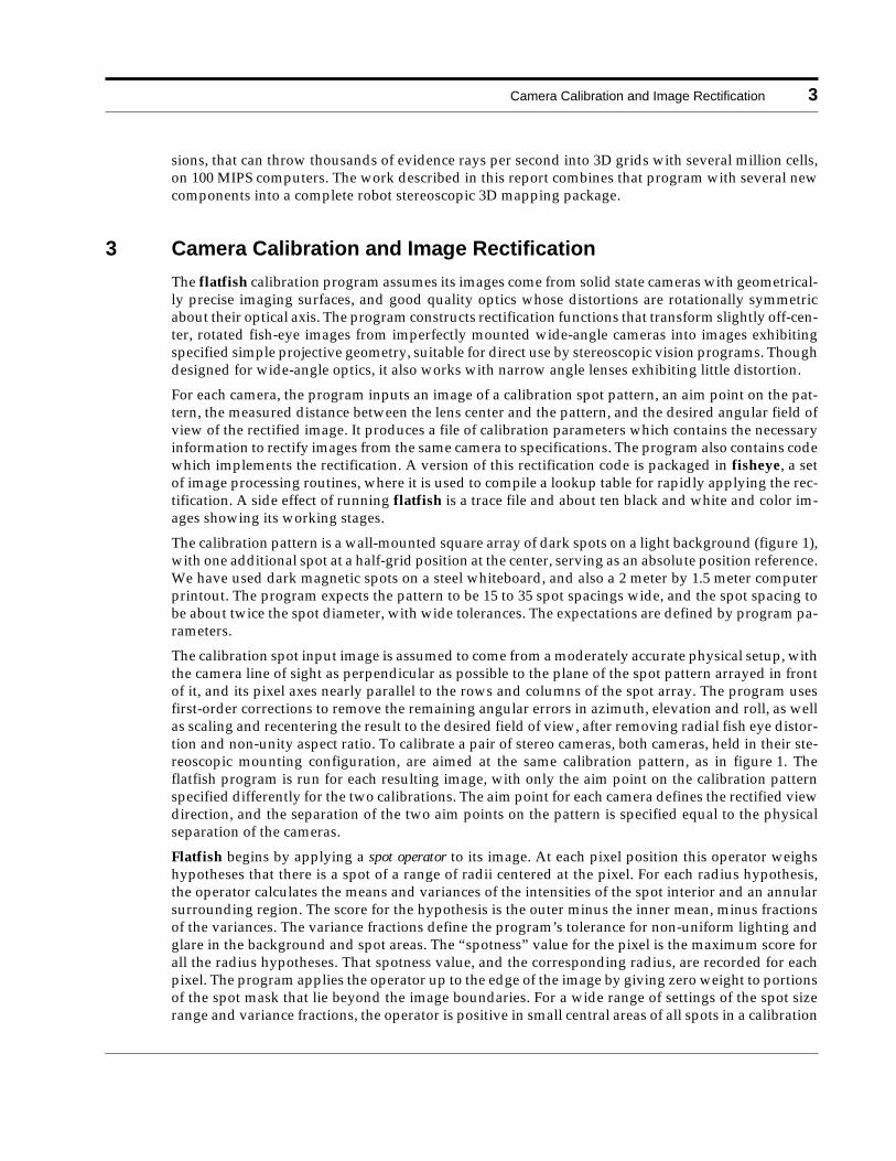
The calibration pattern is a wall-mounted square array of dark spots on a light background (figure 1),with one additional spot at a half-grid position at the center, serving as an absolute position reference.We have used dark magnetic spots on a steel whiteboard, and also a 2 meter by 1.5 meter computerprintout. The program expects the pattern to be 15 to 35 spot spacings wide, and the spot spacing tobe about twice the spot diameter, with wide tolerances. The expectations are defined by program pa-rameters.

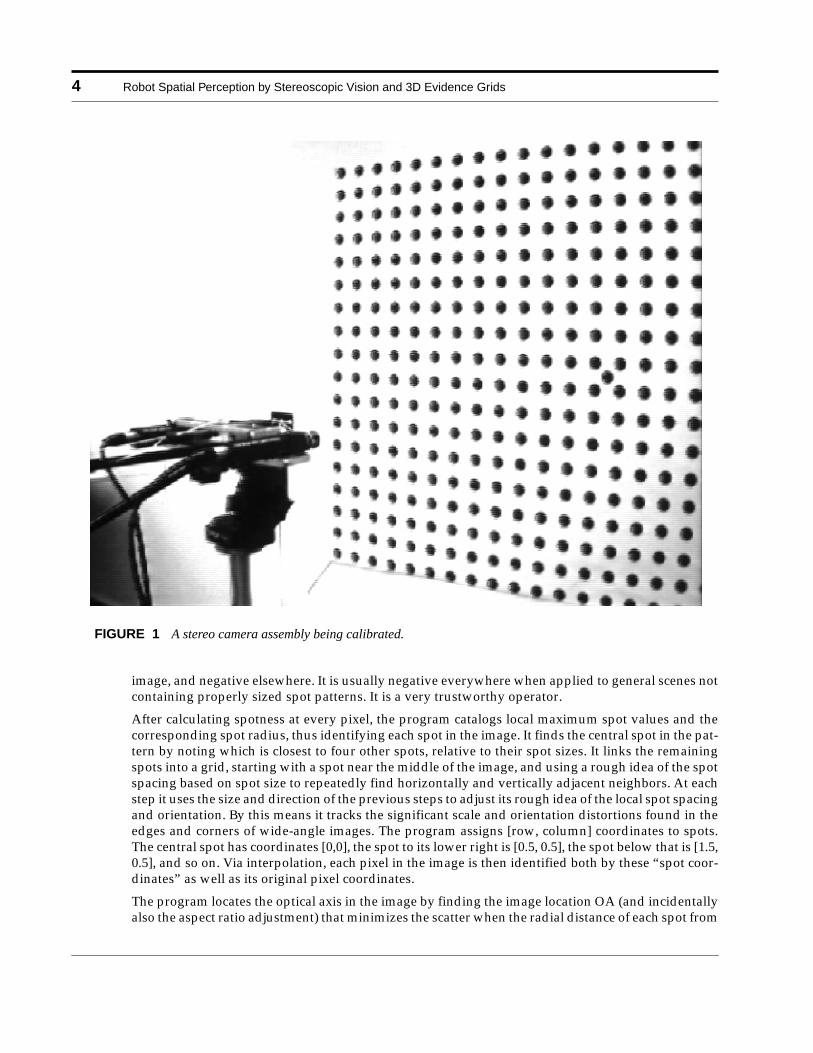
The calibration spot input image is assumed to come from a moderately accurate physical setup, withthe camera line of sight as perpendicular as possible to the plane of the spot pattern arrayed in frontof it, and its pixel axes nearly parallel to the rows and columns of the spot array. The program usesfirst-order corrections to remove the remaining angular errors in azimuth, elevation and roll, as wellas scaling and recentering the result to the desired field of view, after removing radial fish eye distor-tion and non-unity aspect ratio. To calibrate a pair of stereo cameras, both cameras, held in their ste-reoscopic mounting configuration, are aimed at the same calibration pattern, as in figure 1. Theflatfish program is run for each resulting image, with only the aim point on the calibration patternspecified differently for the two calibrations. The aim point for each camera defines the rectified viewdirection, and the separation of the two aim points on the pattern is specified equal to the physicalseparation of the cameras.

Flatfish begins by applying a spot operator to its image. At each pixel position this operator weighshypotheses that there is a spot of a range of radii centered at the pixel. For each radius hypothesis,the operator calculates the means and variances of the intensities of the spot interior and an annularsurrounding region. The score for the hypothesis is the outer minus the inner mean, minus fractionsof the variances. The variance fractions define the program’s tolerance for non-uniform lighting andglare in the background and spot areas. The “spotness” value for the pixel is the maximum score forall the radius hypotheses. That spotness value, and the corresponding radius, are recorded for eachpixel. The program applies the operator up to the edge of the image by giving zero weight to portionsof the spot mask that lie beyond the image boundaries. For a wide range of settings of the spot sizerange and variance fractions, the operator is positive in small central areas of all spots in a calibration


image, and negative elsewhere. It is usually negative everywhere when applied to general scenes notcontaining properly sized spot patterns. It is a very trustworthy operator.

After calculating spotness at every pixel, the program catalogs local maximum spot values and thecorresponding spot radius, thus identifying each spot in the image. It finds the central spot in the pat-tern by noting which is closest to four other spots, relative to their spot sizes. It links the remainingspots into a grid, starting with a spot near the middle of the image, and using a rough idea of the spotspacing based on spot size to repeatedly find horizontally and vertically adjacent neighbors. At eachstep it uses the size and direction of the previous steps to adjust its rough idea of the local spot spacingand orientation. By this means it tracks the significant scale and orientation distortions found in theedges and corners of wide-angle images. The program assigns [row, column] coordinates to spots.The central spot has coordinates [0,0], the spot to its lower right is [0.5, 0.5], the spot below that is [1.5,0.5], and so on. Via interpolation, each pixel in the image is then identified both by these “spot coor-dinates” as well as its original pixel coordinates.

The program locates the optical axis in the image by finding the image location OA (and incidentallyalso the aspect ratio adjustment) that minimizes the scatter when the radial distance of each spot from

FIGURE 1 A stereo camera assembly being calibrated.


OA, measured in pixel coordinates, is plotted against the same radial distance measured in spot co-ordinates. The shape of the spot versus pixel radius curve characterizes the fish-eye distortion, and isrepresented in the program by a least-squares best-fit polynomial. With a 90 degree field of view lens(figure 3), we found that the pixel coordinates of the optimum OA remained stable within a few hun-dredths of a pixel as the camera was moved to various positions in front of a calibration grid. Theroot-mean-square deviation of the pixel versus spot radius scatter diagram, when OA was chosenrandomly near the center of the image was about 2.5 pixels. The rms error was reduced to less than0.5 pixels at the optimum OA.

In another least-squares step, the program then finds and applies the image rotation (roll) that mostnearly makes the fish-eye corrected spot pattern line up with the pixel rows and columns. It also shiftsand scales the image to bring the requested aim point to the exact center, and to provide exactly therequested field of view across the width of the image raster. The largest source of error is probably inthe user’s estimate of the distance between the lens center and the test pattern, which affects the trueangle of view. We use the lens iris ring position as an estimate for the lens center. The uncertaintydiminishes as the pattern and the camera distance are made larger, or the lens is made smaller.

The final result is encoded as parameters for an image rectification program. These parameters areread in before stereoscopic processing, and expanded into rectification tables, which have, for eachpixel in the rectified image, the coordinates of the corresponding source pixel in the raw image. Dur-ing a mapping run, each image digitized by a particular camera is transformed into a rectified imagevia the table corresponding to that camera.

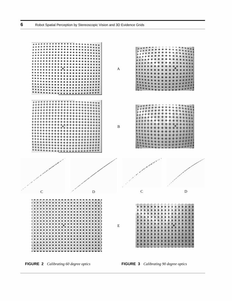
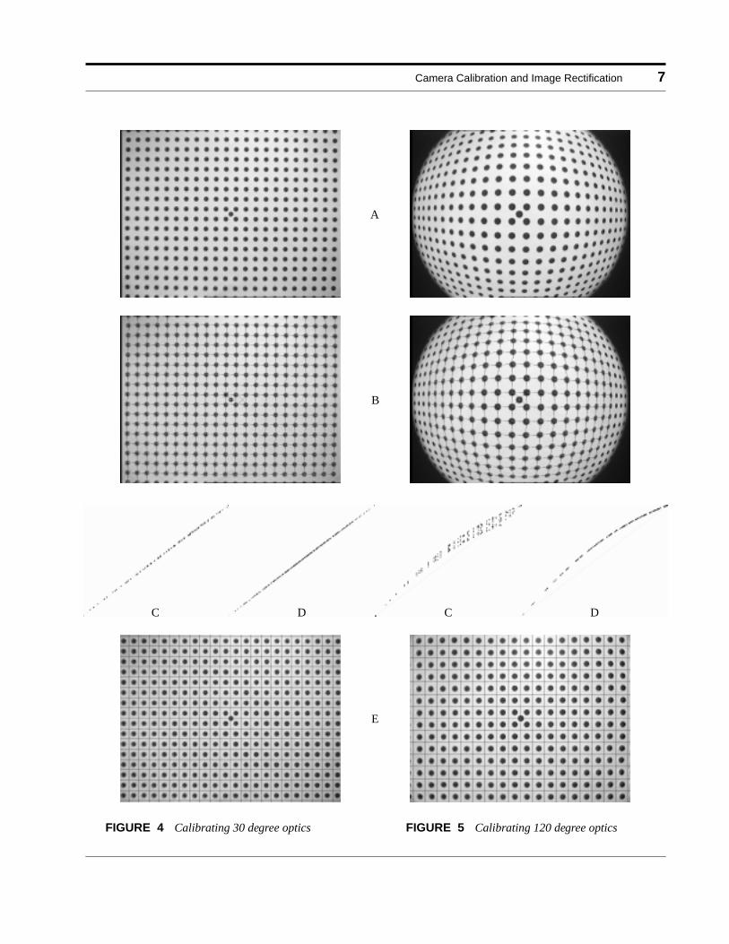
Figures 2, 3, 4 and 5 on the following two pages show the results of applying flatfish to images from60, 90, 30 and 120 degree field of view cameras, respectively. The A figures are the original images, Bshow the regions where the spot operator is positive (small light splotches in the center of the blackspots, visible especially in the isolated center spot), and the coordinate grid resulting from linking thespot operator maxima. The C and D graphs are plots of pixel coordinate radius versus spot coordi-nate radius for all the spots, C for an arbitrarily chosen center marked by a small X on a spot near thecenter in each B image, D from the position that minimized the scatter in the graph, marked by a largeX. The program assumes the scatter-minimizing center marks the true optical axis. The shape of thecurve defined by the scatter diagram is the radial distortion function. The E images are the originalspot image rectified by the function constructed by flatfish, and overlaid with a grid whose spacingshould match the spacing of the spots in the rectified image. Figure 5, derived from an image whosefield of view was 120 degrees, was rectified to only 100 degrees of view, to eliminate the vignettedcorner black areas.


FIGURE 2 Calibrating 60 degree optics FIGURE 3 Calibrating 90 degree optics

A

B

E

C D C D


FIGURE 4 Calibrating 30 degree optics FIGURE 5 Calibrating 120 degree optics

A

B

E

C D C D


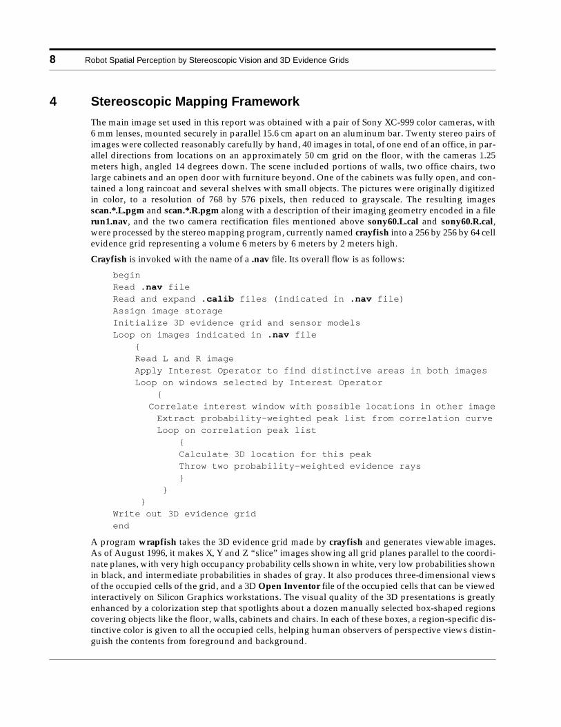
4 Stereoscopic Mapping Framework

The main image set used in this report was obtained with a pair of Sony XC-999 color cameras, with6 mm lenses, mounted securely in parallel 15.6 cm apart on an aluminum bar. Twenty stereo pairs ofimages were collected reasonably carefully by hand, 40 images in total, of one end of an office, in par-allel directions from locations on an approximately 50 cm grid on the floor, with the cameras 1.25meters high, angled 14 degrees down. The scene included portions of walls, two office chairs, twolarge cabinets and an open door with furniture beyond. One of the cabinets was fully open, and con-tained a long raincoat and several shelves with small objects. The pictures were originally digitizedin color, to a resolution of 768 by 576 pixels, then reduced to grayscale. The resulting imagesscan.*.L.pgm and scan.*.R.pgm along with a description of their imaging geometry encoded in a filerun1.nav, and the two camera rectification files mentioned above sony60.L.cal and sony60.R.cal,were processed by the stereo mapping program, currently named crayfish into a 256 by 256 by 64 cellevidence grid representing a volume 6 meters by 6 meters by 2 meters high.

Crayfish is invoked with the name of a .nav file. Its overall flow is as follows:

begin Read .nav file Read and expand .calib files (indicated in .nav file) Assign image storage Initialize 3D evidence grid and sensor models Loop on images indicated in .nav file { Read L and R image Apply Interest Operator to find distinctive areas in both images Loop on windows selected by Interest Operator { Correlate interest window with possible locations in other image Extract probability-weighted peak list from correlation curve Loop on correlation peak list { Calculate 3D location for this peak Throw two probability-weighted evidence rays } } } Write out 3D evidence grid end

A program wrapfish takes the 3D evidence grid made by crayfish and generates viewable images.As of August 1996, it makes X, Y and Z “slice” images showing all grid planes parallel to the coordi-nate planes, with very high occupancy probability cells shown in white, very low probabilities shownin black, and intermediate probabilities in shades of gray. It also produces three-dimensional viewsof the occupied cells of the grid, and a 3D Open Inventor file of the occupied cells that can be viewedinteractively on Silicon Graphics workstations. The visual quality of the 3D presentations is greatlyenhanced by a colorization step that spotlights about a dozen manually selected box-shaped regionscovering objects like the floor, walls, cabinets and chairs. In each of these boxes, a region-specific dis-tinctive color is given to all the occupied cells, helping human observers of perspective views distin-guish the contents from foreground and background.

Interest Operator 9

The flayfish program, derived from crayfish, includes additional code to optimize (learn) good pa-rameters shaping the sensor model that defines the evidence rays. It repeats the crayfish outer loopand its immediate initialization with different settings of sensor model parameters looking for com-binations that maximize a map-quality measure.

Crayfish invokes the separately compiled procedures in files fisheye and volsense. Volsense con-tains code for manipulating 3D evidence grids. Fisheye has procedures for expanding calibrationfiles into rectification tables, and for applying the rectifications to images. It also holds interest operatorand correlator procedures for stereoscopic processing. Following sections describe crayfish’s majorcomponents.

5 Interest Operator

Stereoscopy in crayfish is done by matching small windows in both images of a stereo pair. The po-sition of the matching window in either image defines a 3D ray from the camera, and the relative dis-placement of the window from one picture to the other defines a 3D position along that ray. Theprogram interprets such matches as evidence for the existence of a visible feature in that 3D location.

Not all locations in an image are suitable for matching. Large areas of blue sky or white wall, for in-stance, look identical, as do linear regions along simple edges, with no way to distinguish one partic-ular small patch from a nearby one. An interest operator is applied to an image to select regions likelyto be unambiguously matched in its stereo partner. We invented the concept of the interest operatorin 1974, along with the idea of correlation through a coarse-to-fine image pyramid, and used them inthe first round of work leading to the present results [Moravec81]. Interest operators and image pyr-amid correlation are now widely used in the initial registration steps of digital photogrammetry[Hellwich&al94] [Stunz-Knopfle-Roth94]. Mobile robot stereoscopy is much sloppier than photo-grammetric stereoscopy because robots, immersed in their scene, encounter visual occlusions, per-spective scale and view angle distortions, oblique featureless and specular surfaces, enormous depthratios and other complications.

After a stereo pair of images is rectified, the program applies an interest operator to the left half of theright camera’s image, and to the right half of the left camera’s image. Features chosen from those half-images are most likely to be present in the other camera’s image, while together still covering the fullfield of view. A quirk of the approach is that a narrow stripe the width of the camera separation, run-ning to infinity, is seen in both half images, and thus examined doubly.

The interest operator is a variant of one used in our early research. It subdivides the image into a gridof non-overlapping 8x8 windows, and on each computes the sum of squares of differences of pixelsadjacent in each of four directions: horizontal, vertical and right and left diagonals. The raw interestmeasure for each window is the minimum of these four sums, representing the weakest directionalvariation. If this weakest direction has some contrast, the feature is neither a uniform area nor a sim-ple edge.

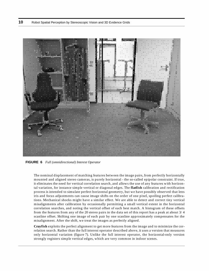
Our 1974 interest operator picked only the local maxima of the raw interest measure. The 1996 pro-gram applies a high pass filter over the array of interest windows, subtracting the average interestvalue of the eight surrounding neighbors from the value of each window. Windows are chosen forranging if they are positive after the high pass operation. The idea in both cases is to cover the imageas uniformly as possible, while picking the best possible features in each area. The 1974 programfound less than 50 features per stereo set, the 1996 program extracts about 2,500 (figure 6).


The nominal displacement of matching features between the image pairs, from perfectly horizontallymounted and aligned stereo cameras, is purely horizontal - the so-called epipolar constraint. If true,it eliminates the need for vertical correlation search, and allows the use of any features with horizon-tal variation, for instance simple vertical or diagonal edges. The flatfish calibration and rectificationprocess is intended to simulate perfect horizontal geometry, but we have possibly observed that lensiris and focus adjustments can cause image shifts on the order of one pixel, spoiling perfect calibra-tions. Mechanical shocks might have a similar effect. We are able to detect and correct tiny verticalmisalignments after calibration by occasionally permitting a small vertical extent in the horizontalcorrelation searches, and noting the vertical offset of each best match. A histogram of these offsetsfrom the features from any of the 20 stereo pairs in the data set of this report has a peak at about 3/4scanline offset. Shifting one image of each pair by one scanline approximately compensates for themisalignment. After the shift, we treat the images as perfectly aligned.

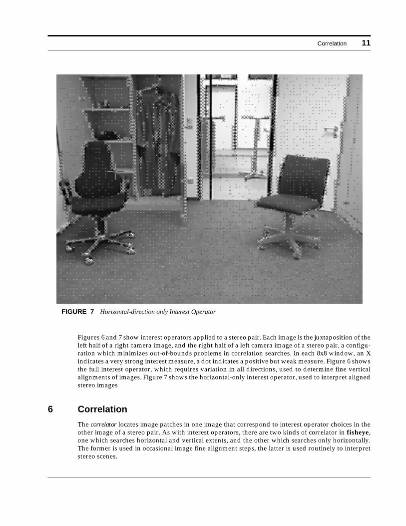
Crayfish exploits the perfect alignment to get more features from the image and to minimize the cor-relation search. Rather than the full interest operator described above, it uses a version that measuresonly horizontal variation (figure 7). Unlike the full interest operator, the horizontal-only versionstrongly registers simple vertical edges, which are very common in indoor scenes.

FIGURE 6 Full (omnidirectional) Interest Operator

Correlation 11

Figures 6 and 7 show interest operators applied to a stereo pair. Each image is the juxtaposition of theleft half of a right camera image, and the right half of a left camera image of a stereo pair, a configu-ration which minimizes out-of-bounds problems in correlation searches. In each 8x8 window, an Xindicates a very strong interest measure, a dot indicates a positive but weak measure. Figure 6 showsthe full interest operator, which requires variation in all directions, used to determine fine verticalalignments of images. Figure 7 shows the horizontal-only interest operator, used to interpret alignedstereo images

6 Correlation

The correlator locates image patches in one image that correspond to interest operator choices in theother image of a stereo pair. As with interest operators, there are two kinds of correlator in fisheye,one which searches horizontal and vertical extents, and the other which searches only horizontally.The former is used in occasional image fine alignment steps, the latter is used routinely to interpretstereo scenes.

FIGURE 7 Horizontal-direction only Interest Operator


Omitting complications, described below, the correlator computes a match value between a patch inone image and a corresponding patch around every pixel position in a search area in the other imageof a stereo pair. In the existing code, the patches are 7x7 pixel squares. Other sizes also work, and soonwe may try circular shapes. The comparison measure is the sum of squares of differences of corre-sponding pixels, with the window means subtracted:

with a and b, implicitly subscripted 1 to n, representing the n pixels in two overlaid windows.

The horizontal-only correlator returns a “match curve” array of correlation values, one for each pixelposition in its search. Traditional stereo programs simply select the best match in such curves, but ourprogram processes multiple candidate matches. The full-area correlator searches a rectangle in an im-age, but returns more information about the horizontal direction. For each horizontal position, itsearches the vertical range for the best match, and returns that value in the “match curve” array. Aparallel array gets the vertical offset that produced that best match.

The known camera separation, position and orientation for each set of rectified images determinesthe bounds of the correlation search and the interpretation of the results. Each candidate match is in-terpreted as a possible 3D surface feature at a particular heading and distance. The evidence raythrower, described in the next section, adds evidence to 3D grids along narrow cones from the camerapositions to the surface feature. With 20 image pairs and 2,500 correlation searches per pair, theamount of evidence accumulated in our 4 million cell grid is substantial, allowing for quite sensitivestatistical evaluations of small changes in the program. A very simple such measure is the count ofthe number of positive cells found in the floor plane of the grid, many produced by weak correlationson the subtle smudges in our uniform gray carpet. About 11,000 floor cells are normally found, butthe number drops rapidly with very small deteriorations of the correlator quality. For instance, if thecorrelation match measure is changed from the means-adjusted version:

to a simple sum of squares of differences:

the number of floor cells drops to about 4,000. Simply rounding the correlation window means from16 to 8 bits reduces the floor count from 11,000 to 7,000.

The means adjustment is not uniformly beneficial. It costs computation in the inner loop, and it dis-cards information about the absolute brightness of windows, sometimes finding a best match be-tween a white patch with a black one. In an experiment with a wider than usual correlation search,where only best matches were considered, for 20 high contrast windows drawn randomly from thedata set, the simple and adjusted measures both made six errors in twenty correlations, but only threein common. In the cases where the simple measure was correct and the adjusted measure wrong, anabsolute brightness difference overrode a spurious similarity in variations. In cases where the adjust-ed was right and the simple wrong, an overall difference in brightness between the pictures overrodea match in subtle contrast. The simple measure fared worse with low contrast windows, making 12errors in 20 against the adjusted’s 10 errors. Still, the simple measure was correct in one low contrastcase where the adjusted measure was in error.

aΣan

------– b

Σbn

------– –

2

∑ a b–( )2∑a∑ b∑–( )2

n----------------------------------–=

a b–( )2∑a∑ b∑–( )2

n----------------------------------–

a b–( )2∑

Correlation 13

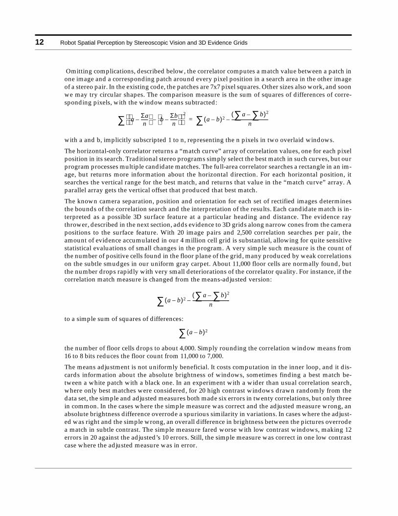
Optical and electronic adjustment differences, and automatic gain changes with changing views, en-sure that the images from the two cameras will rarely match each other exactly in brightness. Sub-tracting out the window means usually improves the correlation by removing such differences.Sometimes it removes too much, and allows a very dark patch to match a very light one. We found asolution to this problem that has the added benefit of speeding up the correlation. A comparison ofthe means of the a and b windows in a correlation can be used as a preliminary discriminant: too dif-ferent, and a match between the windows can be rejected without doing the expensive cal-culation. The means can be precomputed for the entire images very efficiently by a sliding sumtechnique. A preliminary test of the idea showed that about half of the square sums could be elimi-nated by this approach, while the number of errors in the high contrast example above dropped from6 to 4 out of the 20.

FIGURE 8 Correlation of an unanbiguous feature.

Σ a b–( )2


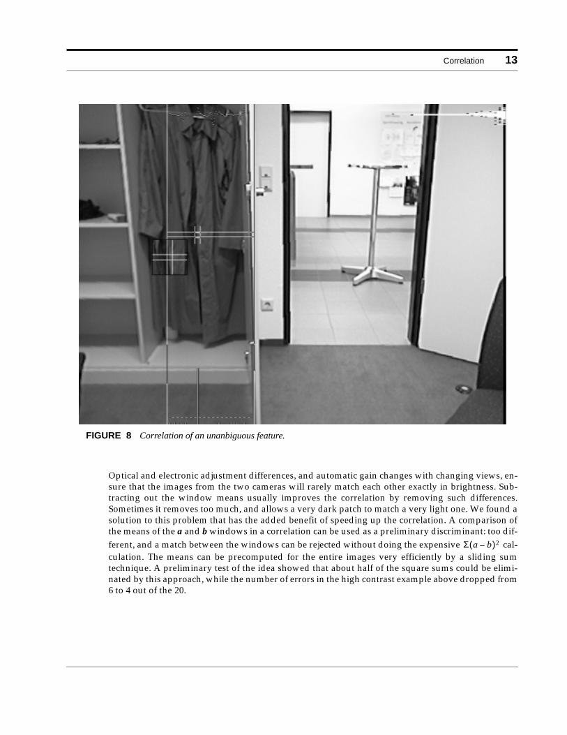
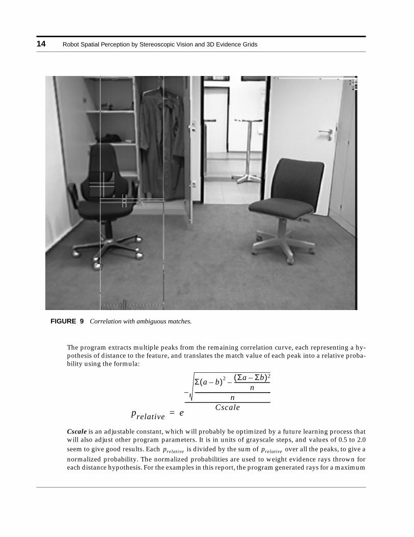
The program extracts multiple peaks from the remaining correlation curve, each representing a hy-pothesis of distance to the feature, and translates the match value of each peak into a relative proba-bility using the formula:

Cscale is an adjustable constant, which will probably be optimized by a future learning process thatwill also adjust other program parameters. It is in units of grayscale steps, and values of 0.5 to 2.0seem to give good results. Each is divided by the sum of over all the peaks, to give anormalized probability. The normalized probabilities are used to weight evidence rays thrown foreach distance hypothesis. For the examples in this report, the program generated rays for a maximum

FIGURE 9 Correlation with ambiguous matches.

prelative e

Σ a b–( )2 Σa Σb–( )2

n--------------------------–

n--------------------------------------------------------–

Cscale---------------------------------------------------------------

=

prelative prelative

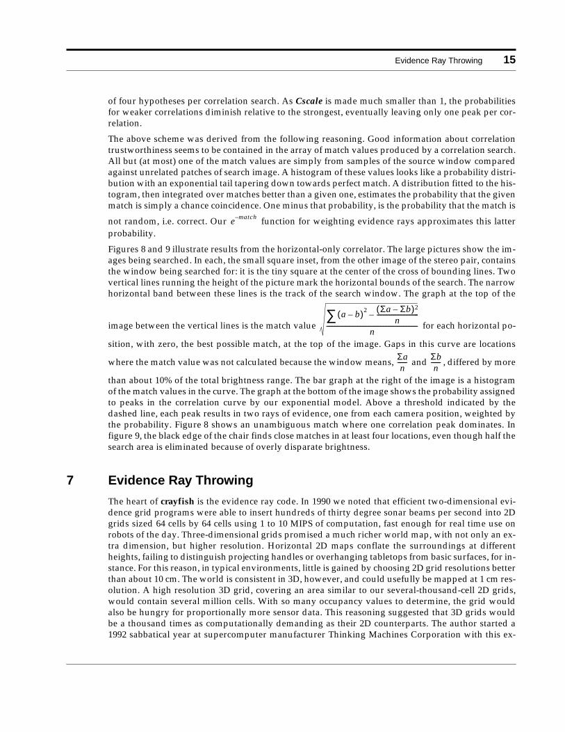
Evidence Ray Throwing 15

of four hypotheses per correlation search. As Cscale is made much smaller than 1, the probabilitiesfor weaker correlations diminish relative to the strongest, eventually leaving only one peak per cor-relation.

The above scheme was derived from the following reasoning. Good information about correlationtrustworthiness seems to be contained in the array of match values produced by a correlation search.All but (at most) one of the match values are simply from samples of the source window comparedagainst unrelated patches of search image. A histogram of these values looks like a probability distri-bution with an exponential tail tapering down towards perfect match. A distribution fitted to the his-togram, then integrated over matches better than a given one, estimates the probability that the givenmatch is simply a chance coincidence. One minus that probability, is the probability that the match is

not random, i.e. correct. Our function for weighting evidence rays approximates this latterprobability.

Figures 8 and 9 illustrate results from the horizontal-only correlator. The large pictures show the im-ages being searched. In each, the small square inset, from the other image of the stereo pair, containsthe window being searched for: it is the tiny square at the center of the cross of bounding lines. Twovertical lines running the height of the picture mark the horizontal bounds of the search. The narrowhorizontal band between these lines is the track of the search window. The graph at the top of the

image between the vertical lines is the match value for each horizontal po-

sition, with zero, the best possible match, at the top of the image. Gaps in this curve are locations

where the match value was not calculated because the window means, and , differed by more

than about 10% of the total brightness range. The bar graph at the right of the image is a histogramof the match values in the curve. The graph at the bottom of the image shows the probability assignedto peaks in the correlation curve by our exponential model. Above a threshold indicated by thedashed line, each peak results in two rays of evidence, one from each camera position, weighted bythe probability. Figure 8 shows an unambiguous match where one correlation peak dominates. Infigure 9, the black edge of the chair finds close matches in at least four locations, even though half thesearch area is eliminated because of overly disparate brightness.

7 Evidence Ray Throwing

The heart of crayfish is the evidence ray code. In 1990 we noted that efficient two-dimensional evi-dence grid programs were able to insert hundreds of thirty degree sonar beams per second into 2Dgrids sized 64 cells by 64 cells using 1 to 10 MIPS of computation, fast enough for real time use onrobots of the day. Three-dimensional grids promised a much richer world map, with not only an ex-tra dimension, but higher resolution. Horizontal 2D maps conflate the surroundings at differentheights, failing to distinguish projecting handles or overhanging tabletops from basic surfaces, for in-stance. For this reason, in typical environments, little is gained by choosing 2D grid resolutions betterthan about 10 cm. The world is consistent in 3D, however, and could usefully be mapped at 1 cm res-olution. A high resolution 3D grid, covering an area similar to our several-thousand-cell 2D grids,would contain several million cells. With so many occupancy values to determine, the grid wouldalso be hungry for proportionally more sensor data. This reasoning suggested that 3D grids wouldbe a thousand times as computationally demanding as their 2D counterparts. The author started a1992 sabbatical year at supercomputer manufacturer Thinking Machines Corporation with this ex-

e match–

a b–( )2∑ Σa Σb–( )2

n---------------------------–

n-----------------------------------------------------------

Σan

------ Σbn

------


pectation, intending to gain some early experience with 3D grids using a CM-5 supercomputer. A se-ries of innovations and approximations, implemented with efficient representations and coding in anintense seven-month programming effort, resulted instead in a program volsense that was about ahundred times faster than anticipated, sufficiently fast for a conventional computer. This speed madecrayfish possible in 1996.

The focal point of volsense is a procedure to add precomputed evidence functions representing sin-gle sensor readings, collectively called a sensor model, to 3D map grids. Each element of a sensor mod-el is a spatial evidence pattern representing the occupancy information implied by a possible reading,for instance a particular range from a sonar ping or stereoscopic triangulation. The evidence accumu-lation operation is a simple integer addition, representing a Bayesian update, with quantities inter-

preted as probabilities in log-odds form, i.e. .

In original conception, the sensor models for 3D grids would themselves be smaller 3D grids, whichwould be positioned and rotated relative to the map grid, corresponding to the position and orienta-tion of the physical sensor. A first innovation noted that almost every sensor we considered, includ-ing sonar, stereo, laser rangefinders and various proximity and touch sensors, could beapproximately represented by evidence patterns symmetric about a view axis. The symmetry allowssensor models to be simple 2D grids, with one dimension radius r from the axis of view, the otherdistance d along it. In use, the rd planes are swept about the axis into cylinders as they are added tothe map grid. A 3D grid map can be seen as a series of xy planes layered in the z direction. An rd cyl-inder intersects successive xy planes in a series of ellipses. The effective z direction can be chosenfrom among the three grid axes to minimize the eccentricity of these ellipses.

If the xy coordinates of each plane are shifted to put its origin at the center of its ellipse, the mappingbetween xy and rd coordinates on successive planes becomes very regular. Each particular xy hasidentical r on successive planes, and its d simply increases by a constant from one plane to the next.This allows an xy -> rd addressing ellipse to be precomputed for one plane, and repeatedly reused tofill the cylinder. With all coordinates precombined into single address words in a table representingthis ellipse, the inner evidence accumulation loop requires only ten single-cycle operations, mostlyinteger additions, per cell updated. This approach is at least 10 times faster than straightforwardlycombining arbitrarily rotated 3D grids.

Another factor of 4 efficiency came from considering only the cells that change the map, typically acone radiating from the sensor. A cone has one quarter the volume of its bounding box. At the timerd sensor models are generated, the sensor model builder also stores a profile of the maximum r ofsignificant data for each d value. For each ray cast, the slice precalculation sorts the xy -> rd address-ing table into increasing r order. The mapping geometry assures each xy slice is updated from a V-shaped wedge in the rd array. For each slice, the evidence accumulation inner loop terminates whenthe r value in the addressing table reaches the profile’s maximum r in the current wedge.

A factor of 2.5 speedup was obtained for “free” from optimization level O3 in the 1992 vintageGnuCC compiler. This was far better than the optimizations provided by earlier compilers of 2D gridprograms. Additional efficiencies occur in the addressing slice precomputation. The xy -> rd table isput into r order by a linear-time bucket sort. The program exploits a four-way skew symmetry in theintersection ellipse, and gets advantages from various coding and incremental computation tech-niques. For the special case of “thin-rays” never more than one grid cell wide, the program employsmuch simpler code, about twice as fast as the general “fat-ray” method described above.

p1 p–------------

log

Evidence Ray Throwing 17

In 1992, on a 25 MIPS Sparc-2 workstation, the program was able to throw about 200 wide-beam so-nar, or 4000 narrow-beam stereo-vision rays per second through a 128x128x128 world. In 1996, on a100 MIPS Sparc-20, the speeds are four times as high.

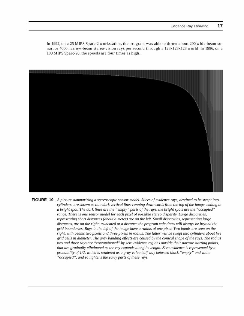
FIGURE 10 A picture summarizing a stereoscopic sensor model. Slices of evidence rays, destined to be swept intocylinders, are shown as thin dark vertical lines running downwards from the top of the image, ending ina bright spot. The dark lines are the “empty” parts of the rays, the bright spots are the “occupied”range. There is one sensor model for each pixel of possible stereo disparity. Large disparities,representing short distances (about a meter) are on the left. Small disparities, representing largedistances, are on the right, truncated at a distance the program calculates will always be beyond thegrid boundaries. Rays in the left of the image have a radius of one pixel. Two bands are seen on theright, with beams two pixels and three pixels in radius. The latter will be swept into cylinders about fivegrid cells in diameter. The gray banding effects are caused by the conical shape of the rays. The radiustwo and three rays are “contaminated” by zero evidence regions outside their narrow starting points,that are gradually eliminated as the ray expands along its length. Zero evidence is represented by aprobability of 1/2, which is rendered as a gray value half way between black “empty” and white“occupied”, and so lightens the early parts of these rays.


8 Constructing Stereo Rays

In 1992 volsense contained a procedure for constructing sensor models inspired by our sonar expe-riences. A sensor model was shaped by 15 parameters, designed to be adjusted by a learning process,controlling evidence cone angle, depth of empty interior, height and thickness of occupied range sur-face, and how these values changed with distance.

Stereoscopic ranging fit the generic model poorly. Stereo distances and uncertainties are well definedby the geometry of the stereo triangulation. A procedure for constructing stereo-specific sensor mod-els was added to volsense. The models it generates contain one evidence pattern for each possiblestereo disparity. The beam angle can be varied from that representing a single image pixel, to thewidth of a correlation window. The examples in this paper were generated with the latter setting. Thedepth range uncertainty is geometrically derived assuming a single horizontal pixel of correlationuncertainty. The evidence rays have a hand-chosen negative occupancy evidence from the imagingposition to the beginning of the range uncertainty region, and a much stronger positive value alongthe region, diluted by the volume of uncertainty. These parameters and many others will be grist fora future learning process, which will vary them to produce better 3D grid maps. Figure 10 shows agraphic representation of a stereoscopic sensor model.

Crayfish throws two rays for each correlation peak, one from each camera position, intersecting attheir calculated range. Multiple hypotheses derived from a correlation curve are translated into mul-tiple superimposed pairs of rays. The evidence in each pair is weighted by its match probability. Thisis accomplished efficiently by selecting one of several precomputed sensor models with variously di-minished evidence values. We typically configure the program to generate 8 or 16 complete sensormodels, coarsely representing probabilities 0 to 1.

9 Program Speed

On a 100 mips Sparc 20, a typical run of crayfish reports the following average timings per stereo pairprocessed for the program’s major steps. Each pair generates about 2,500 correlations, each resultingin 2 to 8 evidence rays, depending on cscale, and limited by another program parameter.

Rectification of two images: 0.2 seconds

Interest Operator: 0.1 seconds

Correlator: 0.9 seconds

Ray Throw: 0.7 to 2.5 seconds, depending on cscale

10 The Office Scan

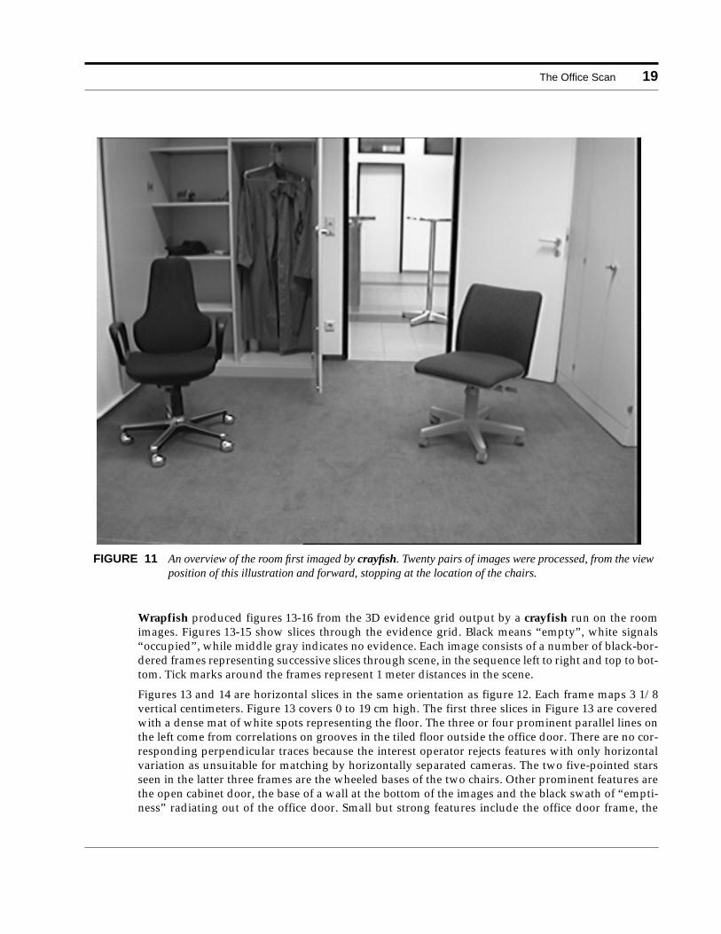
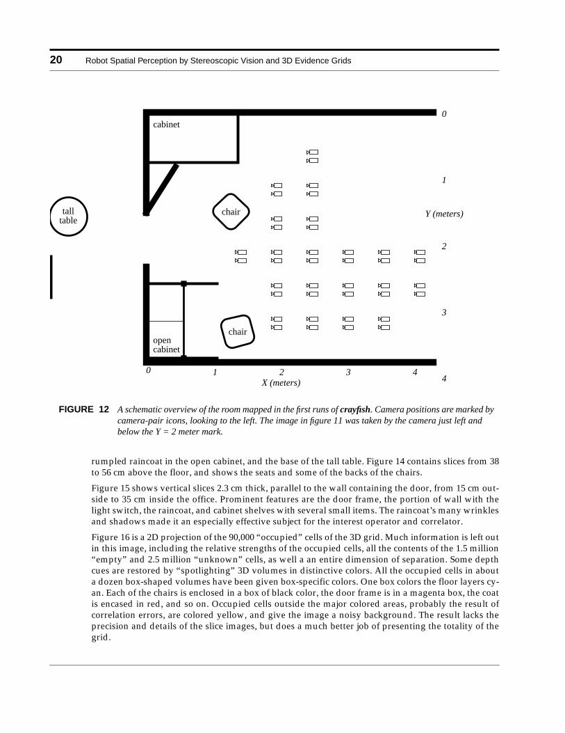
Crayfish was developed with a data set collected using a pair of Sony XC-999 color cameras, with 6mm lenses, mounted securely in parallel 15.6 cm apart on a tripod-mounted aluminum bar. Twentystereo pairs of images were collected reasonably carefully by hand of one end of an office, in paralleldirections, from locations on an approximately 50 cm grid on the floor, with the cameras 1.25 metershigh, angled 14 degrees down. Figure 11 is a view from the back of the data set, and encompassesmost of the scene. Figure 12 shows the placement of the cameras in the room.

The Office Scan 19

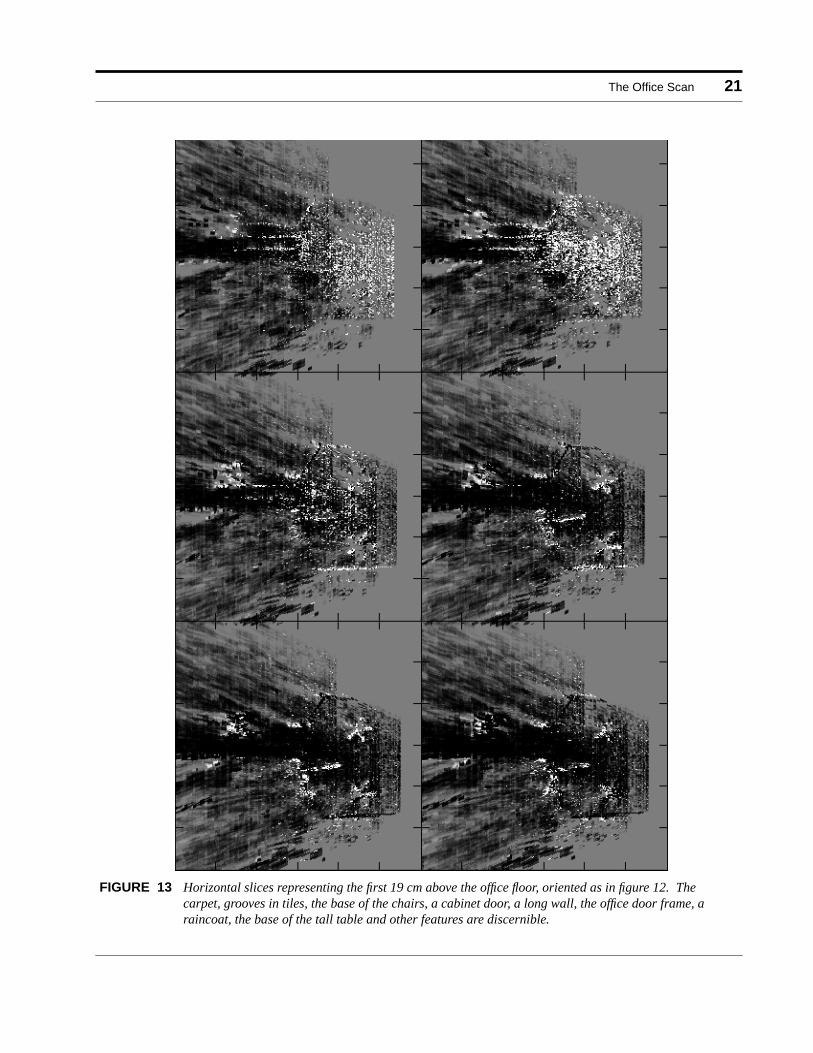
Wrapfish produced figures 13-16 from the 3D evidence grid output by a crayfish run on the roomimages. Figures 13-15 show slices through the evidence grid. Black means “empty”, white signals“occupied”, while middle gray indicates no evidence. Each image consists of a number of black-bor-dered frames representing successive slices through scene, in the sequence left to right and top to bot-tom. Tick marks around the frames represent 1 meter distances in the scene.

Figures 13 and 14 are horizontal slices in the same orientation as figure 12. Each frame maps 3 1/8vertical centimeters. Figure 13 covers 0 to 19 cm high. The first three slices in Figure 13 are coveredwith a dense mat of white spots representing the floor. The three or four prominent parallel lines onthe left come from correlations on grooves in the tiled floor outside the office door. There are no cor-responding perpendicular traces because the interest operator rejects features with only horizontalvariation as unsuitable for matching by horizontally separated cameras. The two five-pointed starsseen in the latter three frames are the wheeled bases of the two chairs. Other prominent features arethe open cabinet door, the base of a wall at the bottom of the images and the black swath of “empti-ness” radiating out of the office door. Small but strong features include the office door frame, the

FIGURE 11 An overview of the room first imaged by crayfish. Twenty pairs of images were processed, from the viewposition of this illustration and forward, stopping at the location of the chairs.


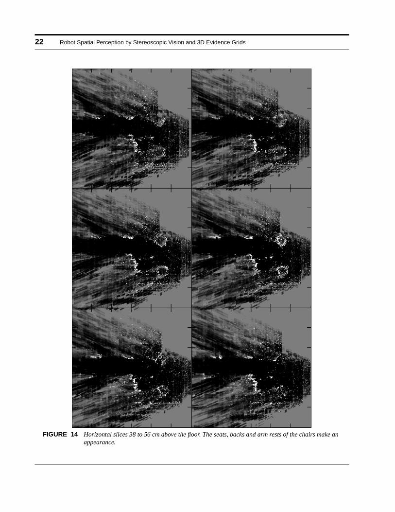
rumpled raincoat in the open cabinet, and the base of the tall table. Figure 14 contains slices from 38to 56 cm above the floor, and shows the seats and some of the backs of the chairs.

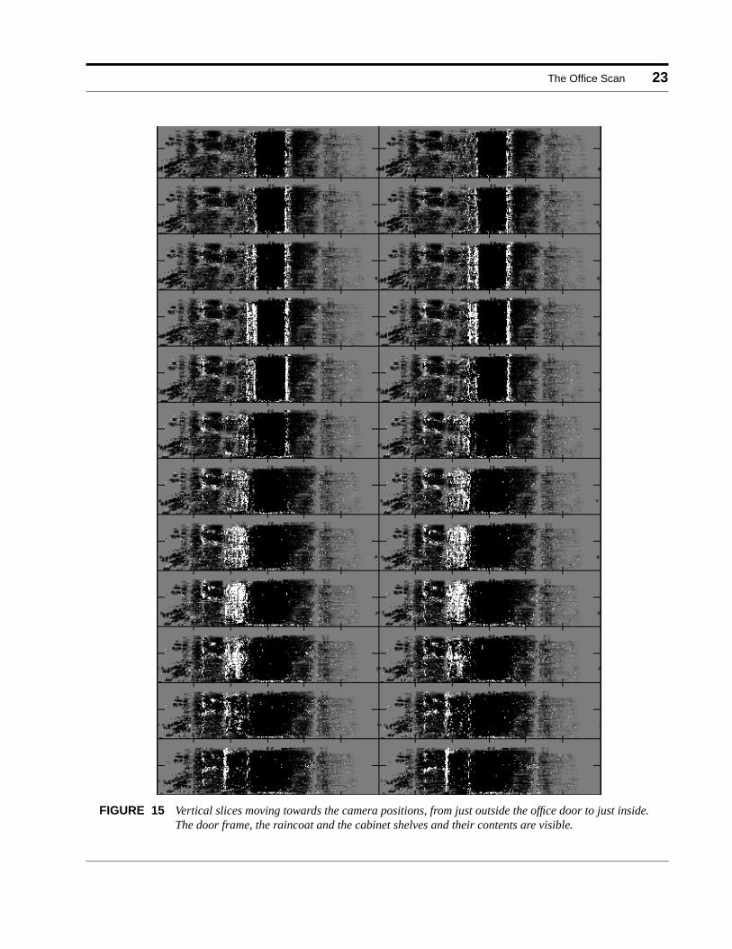
Figure 15 shows vertical slices 2.3 cm thick, parallel to the wall containing the door, from 15 cm out-side to 35 cm inside the office. Prominent features are the door frame, the portion of wall with thelight switch, the raincoat, and cabinet shelves with several small items. The raincoat’s many wrinklesand shadows made it an especially effective subject for the interest operator and correlator.

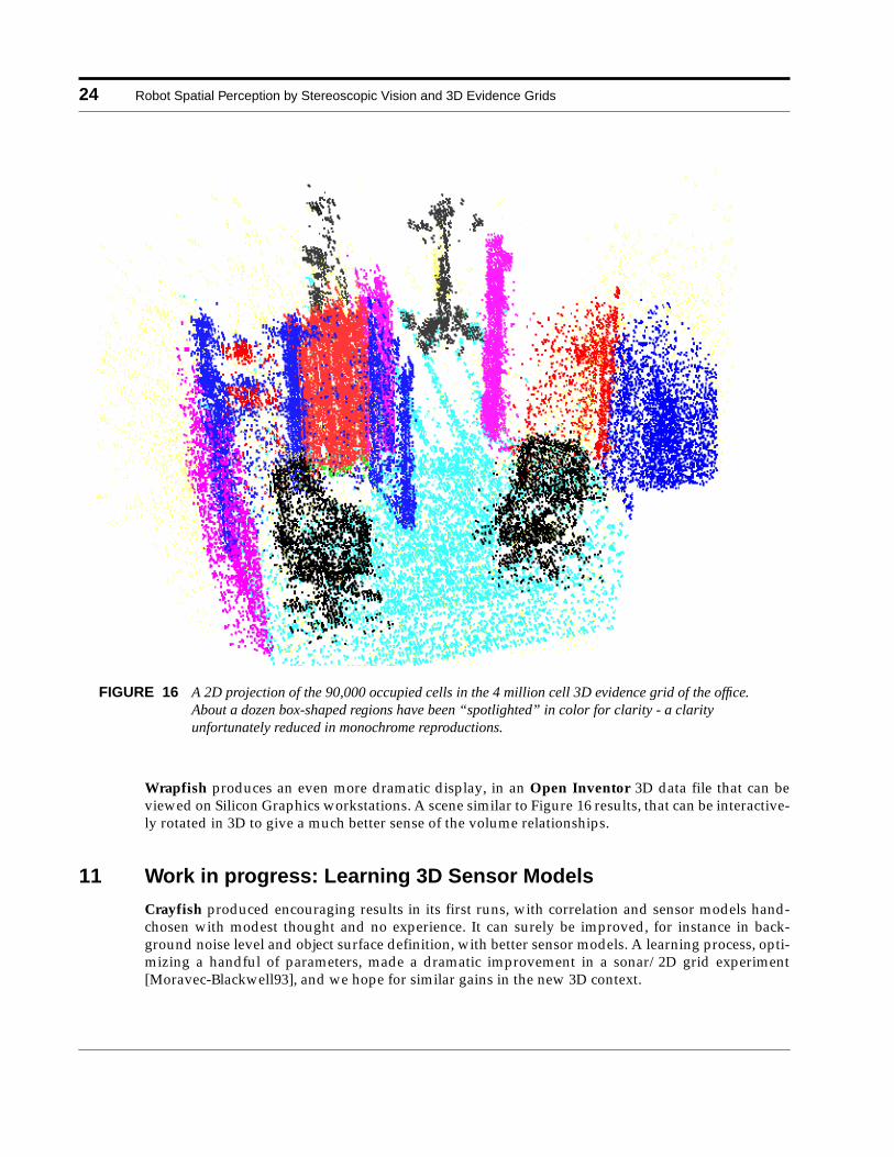
Figure 16 is a 2D projection of the 90,000 “occupied” cells of the 3D grid. Much information is left outin this image, including the relative strengths of the occupied cells, all the contents of the 1.5 million“empty” and 2.5 million “unknown” cells, as well a an entire dimension of separation. Some depthcues are restored by “spotlighting” 3D volumes in distinctive colors. All the occupied cells in abouta dozen box-shaped volumes have been given box-specific colors. One box colors the floor layers cy-an. Each of the chairs is enclosed in a box of black color, the door frame is in a magenta box, the coatis encased in red, and so on. Occupied cells outside the major colored areas, probably the result ofcorrelation errors, are colored yellow, and give the image a noisy background. The result lacks theprecision and details of the slice images, but does a much better job of presenting the totality of thegrid.

talltable

chair

chairopencabinet

cabinet

0 1 2 3 4X (meters)

0

1

2

3

4

Y (meters)

FIGURE 12 A schematic overview of the room mapped in the first runs of crayfish. Camera positions are marked bycamera-pair icons, looking to the left. The image in figure 11 was taken by the camera just left andbelow the Y = 2 meter mark.

The Office Scan 21

FIGURE 13 Horizontal slices representing the first 19 cm above the office floor, oriented as in figure 12. Thecarpet, grooves in tiles, the base of the chairs, a cabinet door, a long wall, the office door frame, araincoat, the base of the tall table and other features are discernible.


FIGURE 14 Horizontal slices 38 to 56 cm above the floor. The seats, backs and arm rests of the chairs make anappearance.

The Office Scan 23

FIGURE 15 Vertical slices moving towards the camera positions, from just outside the office door to just inside.The door frame, the raincoat and the cabinet shelves and their contents are visible.


Wrapfish produces an even more dramatic display, in an Open Inventor 3D data file that can beviewed on Silicon Graphics workstations. A scene similar to Figure 16 results, that can be interactive-ly rotated in 3D to give a much better sense of the volume relationships.

11 Work in progress: Learning 3D Sensor Models

Crayfish produced encouraging results in its first runs, with correlation and sensor models hand-chosen with modest thought and no experience. It can surely be improved, for instance in back-ground noise level and object surface definition, with better sensor models. A learning process, opti-mizing a handful of parameters, made a dramatic improvement in a sonar/2D grid experiment[Moravec-Blackwell93], and we hope for similar gains in the new 3D context.

FIGURE 16 A 2D projection of the 90,000 occupied cells in the 4 million cell 3D evidence grid of the office.About a dozen box-shaped regions have been “spotlighted” in color for clarity - a clarityunfortunately reduced in monochrome reproductions.

Things to Twiddle 25

Automatic learning requires a criterion to optimize. In the sonar/2D example we were able to hand-construct an “ideal map”, or ground-truth model, against which reconstructed grids were compared.The 2D ideal was simple, containing only a few walls and doors at low resolution. The same approachis impractical in our high resolution 3D scenes, which contain tens of thousands of tiny details at thescale of the grid. Ground truth could perhaps have been derived from a high quality scanning laserrangefinder, but none was available while our scenes existed, nor is it now.

Several weeks of experimentation failed to produce a good learning criterion among measures thatcompute various kinds of local solidity in the grid data. Some drove the grid to zero density, othersfilled it with noise. Some had parameters that could be adjusted between these extremes, or to achievesome specified average density, but none were convincingly measures of the correct answer. We con-sidered hand-massaging the best 3D grids encountered to stand in for ground truth, but a morebroadly useful approach has suggested itself.

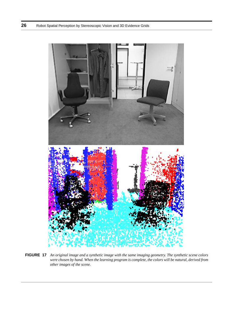
There is a kind of ground truth in the original images of the scene, albeit in 2D projection and withsurface color. The grid, on the other hand, is 3D, and has no color. It is easy to project the grid’s 3Dcells into 2D pictures (figure 17), recreating the geometry of the original images, but without color thegrid projections convey little information. But original colors for the grid can also be obtained fromthe images!

We plan to evaluate trial 3D grid maps by dividing the images from which they were derived into a“coloring” set and an “evaluation” set. In the 20-pair office data, images from more forward positionsare probably best for coloring, and those looking from the back for evaluation.

We will scan the 3D grid from far to near and make a list of positive (“occupied”) cells in scan order.Typically there are a manageable 90,000 occupied cells out of the 4 million total cells. Each elementof this list will get the grid coordinates of the cell, and also an, initially blank, “cell color”.

The cells in the list will be rendered into the viewing geometry of each of the “coloring” images, pro-ducing corresponding synthetic images, with each pixel indicating the identity of the closest occu-pied cell visible at that position, or nothing, if no cell projects there. The program will scan thesynthetic images, and, at each non-empty pixel, average the color of the corresponding location in its“coloring” image into the “cell color” variable of the indicated cell. When done, each cell in the “oc-cupied” list will have an associated color, averaged over the images in which its was visible.

Then the program will project the newly colorized grid into the geometry of the “evaluation” images,and compute similarity. The similarity test is like the colorization, but instead of averaging the orig-inal image color with the cell color, the two are compared.

The evaluation is very similar to a human test of a reconstructed grid: it asks the question, “does itlook right?”. The approach uses information, and measures interesting qualities, in the source imagesnot used in constructing the original grid. For the initial implementation, we will probably use mono-chrome images, averaged down to half size, to do the (grayscale) coloring and evaluation. Color im-ages also exist, and we could use those later. A very interesting side benefit of the colorization processis a grid with the original scene colors, which should be exciting to view.

12 Things to Twiddle

The 3D sensor-grid’s many unexplored directions will surely provide years of amusement. A work-ing learning process and a sensitive map-quality criterion will provide the opportunity to optimizeall parts of the process.


FIGURE 17 An original image and a synthetic image with the same imaging geometry. The synthetic scene colorswere chosen by hand. When the learning program is complete, the colors will be natural, derived fromother images of the scene.

Things to Twiddle 27

Many variations in the basic stereoopsis suggest themselves. Would it be better to preprocess the im-age for features like edges? Should the correlation window be round to maximize the number of pix-els for statistical significance, while minimizing the distance from the center? Should the windows betaller than wide, because a horizontal change in viewpoint causes more horizontal than vertical im-age variation? Should they vary in size? Would pre-adjusting the brightness and contrast of the im-ages on the basis of the strong correlations improve the weak correlations? How would this interactwith the brightness-difference cutoff threshold in the correlation search? Could the minimum dis-tance considered in correlation searches for weak features be modified from image to image, or evenregion to region, on the basis of strong correlations from the same area? The search costs and errorrates are minimized if the search is narrowed as much as possible. How much improvement can beachieved by using other interest operators? Should they return more or fewer points? What about dif-ferent comparison measures? How should evidence rays be weighted as a function of correlationquality? And many more.

Even more fundamental to the grid function is the sensor model, i.e. the shapes and weights of theevidence rays. The existing program uses a very simple, ad hoc sensor model for stereo evidence. Anevidence ray, which is often a line, but can become a cone a few cells in diameter, consists of a hand-picked negative value from the camera to the region of stereo range uncertainty, followed by a posi-tive value covering the length of the uncertainty. The positive value is another hand-chosen constantdivided by the size of the positive volume. The weights are scaled by the correlation probability. Theevidence grid approach derives trustworthy conclusions from very noisy data by accumulating largeamounts of it for each spatial location. The accumulation process is compromised if the individualevidences have systematic biases. A good sensor model is a bias-free representation of the averagetrue information from each kind of measurement. A learning process that adjusts angles, weights, siz-es, shapes, dependence on distance and correlation and many other subtleties should converge onsuch a sensor model. Our simple hand-picked model is unlikely to be very close.

For some purposes, including producing synthetic images, it is necessary to classify evidence valuesinto empty, occupied and unknown. The threshold values for these classifications could be optimizedduring learning.

Some important improvements are beyond the reach of simple learning. This report’s data set wascollected by hand, with tripod mounted cameras. The camera positions cameras varied at least a frac-tion of a centimeter from nominal, and the pan and tilt angles may have varied by more than one de-gree. The latter errors, especially, mean measurements from different views were not perfectlyregistered. Images from moving robots are likely to have even larger position and orientation uncer-tainties. We and others [Yamauchi96], [Schultz-Adams-Grefenstette96] have had good success in pastregistering sonar/2D grids of the same area made from viewpoints, whose relationship is knownonly approximately, by searching for best map match over a range of relative positions and orienta-tions. The large number of cells in the grids allow registration accurate to a fraction of a cell, by inter-polation of the discrete matches. This works even when one of the grids is built with only a few dozensonar readings from a single robot position. The statistically stabilizing multitude of cells in the 3Dgrids assures us that the approach will work even better there. The only question is speed: our gridhas four million cells, and a search over large ranges of 6 degrees of freedom could easily take trillionsof computations! Fortunately there are many strategies for enormously reducing the cost. For a mo-bile robot on a flat floor, only 3 degrees of freedom vary very much, so the search extent in the otherthree can be very small. Even the unconstrained position and angle searches can be kept small by us-ing dead-reckoning information. The search can be reduced almost to its logarithm, by a coarse-to-fine strategy, where approximate answers are computed first at the small end of a pyramid of shrunk-en grids. Coarse-to-fine has worked very well for us in past, in unconstrained stereoscopic correlationand in matching 2D grids. Well-chosen samples could substitute for the whole: for instance, the un-


known areas of a grid could be skipped, or the occupied cells of one grid could be mapped to the en-tirety of the other. A branch and bound strategy might cut short some of the comparisons, when theiraccumulating partial errors exceed the best previous comparison, a method that works best if themost likely registrations are searched first.

We hope to implement an image-pair to scene registration step soon after the learning code is work-ing. It is likely to tighten up the office scene, and will prepare the way for stereo/3D grid use on realrobots.

13 Hardware Helpers

Quirks in our office scene reconstruction suggest some easy hardware alterations likely to significant-ly improve performance. The dense coverage the correlator obtains on the slightly textured carpet,and more heavily textured raincoat, compared to its sparseness on plain surfaces like doors andwalls, suggests that coverage would be greatly increased by the artificial addition of texture acrossthe scene. This could be accomplished simply by mounting a randomly textured floodlight with thecameras, perhaps infrared to minimize effects on humans.

More speculatively, wide angle sonar could provide the range to the nearest feature in the scene, tonarrow the correlation search to that range and beyond, boosting speed and accuracy. A preliminarystereoscopic preprocessing of strong features might give similar information without extra hardware.

Precise image rectification allows the correlation search to be exclusively in the direction of the axishorizontal joining the two cameras. The points to be searched for, selected by an interest operator,need thus have only horizontal variations. As a result, the program picks out a dense coverage of fea-tures along vertical wall and furniture boundaries, but entirely misses the horizontal boundaries.This problematic blindness could be eliminated by adding a third camera to the stereo pair, verticallydisplaced from the original two. The trio could be used in pairs, with points selected by interest op-erators specific to each pair’s separation direction.

The 60 degree field of view cameras, though placed on most of the open floor area of the office, sawonly a tiny portion of the left wall and none of the right, and viewed other elements of the scene froma very narrow range of angles. The grid might be much enhanced if objects were viewed from manydirections. Wider angle lenses would help, as would panning the cameras from side to side duringoperation, or having several camera pairs looking in different directions. The latter option is probablybest, as manufacturers begin to market high quality, inexpensive single-chip cameras with integratedoptics, for applications like hand-held videoconferencing. Simply processing more images wouldalso help, which will surely happen when the cameras are used on a mobile robot that can acquirenew sets of images perhaps every second.

Before the fast ray-throwing code was written, speed seemed the bottleneck for 3D grids. Now cray-fish is quite speedy, but encounters memory limits. Experiments with existing data and small gridextents (see the appendix) show that scene details improve as grid cell size is reduced, even to below1/2 centimeter. The speed cost for increased resolution is modest. For a wide range resolutions, moststereo rays remain one cell in width, and the time to throw rays grows only slightly more than linear-ly with grid resolution. The image processing steps are unaffected, so total runtime grows perhaps50 percent per resolution doubling. Memory usage, on the other hand, grows dramatically. Our256x256x64 grid has four million two-byte cells, consuming about half the program’s 16 megabytes.Doubling the resolution balloons the grid to 64 megabytes. Lowering the cell size to 1/2 centimeterwould require a gigabyte of grid. Memory costs are dropping, and sizes increasing with a time con-stant of about 2 years, so even such numbers should soon be within reach. It’s comforting to know

Future Extensions and Applications 29

that the existing approach will produce even better results in future, simply through hardwareprogress.

14 Future Extensions and Applications

Crayfish builds 3D maps from a set of image files, a first step to myriad goals. Its descendents willprocess real-time images from moving robots. The robots will use their 3D understanding of the sur-roundings to navigate confidently, to locate and interact with objects, eventually to plan and executecomplex tasks involving locomotion and manipulation. To do all that, they will need application pro-grams to extract specific answers from the 3D grids. Here are few answer extractors on our “to do”list:

14.1 Obstacle avoidance Our 3D grids contain over 100 times as much information about robot surroundings as the 2D mapsor sparse 3D models derived by previous mobile robot programs. Since robots can be made to ma-neuver reasonably well with the sparser information, we have very high expectations for 3D-gridbased local navigation. In particular, corners, horizontal projections and inconveniently placed smallobstacles, that can be missed or misinterpreted by the simpler approaches, sometimes with seriousconsequences, appear clearly and unambiguously, in shape and position, in a 3D grid, ready to benoticed by a path-planning program. Finding paths in a 3D grids need not be extremely computation-ally costly. Since the grid specifically marks empty volumes, the frequent case of an unimpeded pathfrom source to local destination can be quickly detected, by sweeping a 3D grid volume in the shapeof the robot along a straight path in the 3D map. The collision probability at each position is found bymultiplying the products of occupancy probabilities of corresponding map and robot cells. The outerproduct becomes a more tractable a sum by taking the logarithm of the inner products. This compu-tation can be made very cheap by a coarse-to-fine strategy, which refines the resolution only for thosefew cells where coarse comparison detects a possible conflict. A full path planner could be construct-ed by embedding such a measure in an A* search. By doing its work in 3D, the planner could producepaths that scoot the robot under overhangs and squeeze its shape through commensurate gaps.

14.2 NavigationNearly every indoor mobile robot task requires the robot to return to previous locations. Existingcommercial delivery and cleaning robots do this with the help of buried wires, wall or floor mountedbeacons or markers, or painstaking handmade site-specific maps of walls and openings, whose fre-quent encounter corrects odometric dead-reckoning. Experimental robots that navigate with auton-omously made 2D maps (e.g. [Koenig-Simmons96], [Schultz-Adams-Grefenstette96], [Yamauchi96]),are not quite reliable enough for commercial use, which demands months of operation without nav-igational failure. Using million-cell 3D maps, with 100,000 surface cells, instead of thousand-cell 2Dmaps, containing at most a few hundred surface points, should decrease the failure probabilitiesenormously. Suppose we want a robot to autonomously repeat routes shown it on a guided tour.During the tour, the robot would build and store a sequence of 3D map “snapshots” of the journey.When on its own, it would match these snapshots against its fresh 3D. The relative position and ori-entation of best match would tell the robot its location relative to its tour route--to a fraction of a cell,if it interpolates. The matching can be done efficiently using the same coarse-to-fine and selectivesampling techniques suggested in the last section for precisely registering new data to old in a devel-oping map. The 3D grids contain so huge a mass of detail, at large and small scales, that the proba-


bility of a good match between two maps of the same area, at other than the correct placement, shouldbe astronomically small. By contrast, with simple line maps or blurry 2D grid maps, the probabilityof a false match, and consequent serious navigational error, is significant. Enormous reduction innavigational and shape confusion probabilities is a major 3D grid promise.

14.3 Object recognitionVolumetric matching, as suggested for navigation, might also be used at smaller scales, and possiblyhigher resolutions, to detect objects by shape. Grid prototypes of objects can be matched to map areasin the same way maps are matched to each other. At a given resolution, the number of cells in a smallobject, and thus the reliability of the match, will be lower. Reliability can be improved by increasingthe grid resolution, in an approach we may call “fine-to-finer”. Stereoscopic data collected for navi-gation can be used again to map small volumes at sub-centimeter resolution, as shown by the chairexample in the appendix. There are complications. Office chairs, for instance, have parts that movewith respect to one another. The back, seat and base of the chair could be sought volumetrically sep-arately, and their match values combined in a formula, with measures of the relative geometric posi-tions, in a hybrid “chair operator” that could be applied to likely positions in the scene. Scene colorscould also weigh in the formula. Experience may suggest a bag of such recognition techniques, whichcan perhaps be orchestrated by an object description language, to conveniently construct operatorsfor even changeable objects like chameleons. A similar approach should work for general navigation.Experience with the language may then suggest how to automate the object and route descriptionprocesses.

14.4 Scene MotionThe data sets for crayfish were accumulated over several hours, with no regard to intervening chang-es in the scene. If there had been changes, the “before” and “after” states would have been averagedtogether. At each location, the program accumulates a weight of evidence of occupancy. If a givenlocation has been identified as occupied many separate times, this weight can become very large. Ifa physical scene rearrangement subsequently empties the location, it will take very many additionalobservations to erase the weight in the grid, and replace it with a negative one. We could deal withoverly persistent memories by a deliberate “forgetting” process. As each update is made, affectedcells would have a small proportion of their old evidence trimmed, thus exponentially decaying ev-idence over the number of sensings of an area, and giving new measurements relatively higherweight. An object moving through a repeatedly sensed area would then show up as a fading streakin the grid, just like the slow-phosphor trail of a moving object on an old-style radar screen. Decayover sensings would leave recently unsensed map areas unchanged. There are reasons to decay thosealso, but probably at a different rate. If, in its wanderings, the robot steadily accumulates navigationalerrors, the registration of very old data with new will become uncertain. This could be accounted forby spatially blurring the old data - we have demonstrated this in 2D grids [Elfes87]. All these tech-niques will become more effective as increasing computer speed allows us to do more frequent sens-ings. With 500 MIPS, it should be possible to process stereo images about once per second. Whencomputer power and memory several times greater becomes available, it will become possible to takethe grid idea into the fourth dimension, with 4D grids representing the local spacetime. Doing sowould replace motion blurs with a stack of instantaneous frames of the scene, from which detailedmoving object dynamics could be derived. For the next several years, however, we will have ourhands full with 3D grids.

Conclusion 31

15 Conclusion

Since 1984, two-dimensional grids have proven effective in turning mobile robot sense readings intoreliable maps, even when individual readings are very ambiguous or noisy. The grid approach cata-logs the surroundings by location, a division independent of individual measurements or their er-rors, allowing arbitrarily many individual readings to be accumulated before any conclusions needbe drawn. It tames sensor noise with large-number statistics. Most competing approaches are muchless tolerant of noise, because they must decide on interpretations, for instance about surfaces, withfar less data. The grid approach threatened to require more memory and computation than priormethods, but its simplicity and regularity allow very efficient implementations. Many experimentalmobile robots today are controlled by real-time 2D grid programs.

Two dimensional grids offer, at best, a blurry view of a slice of the world. We have considered thema prelude to 3D grids, which could represent the complete surroundings in precise detail, and consti-tute the basis of a high-quality robotic sense of space. Their apparent 1,000 times higher computation-al cost delayed the effort to try 3D until 1992, when a supercomputer became available. Work towardsa supercomputer implementation produced instead a surprisingly fast uniprocessor program for thekey 3D evidence-ray throwing step. A complete prototype 3D system, described in this report, wasfinally completed in 1996.

Though it uses unoptimized ad-hoc sensor models, the 3D grid program clearly demonstrates the ef-fectiveness of the approach, and that 500 MIPS would suffice for a real-time version. From stereo-scopic range data with 20 to 50 percent errors, it constructs maps that, imaged, look like doll-housereplicas of the sensed area. The existing program is good enough to feed a highly reliable robot nav-igator, but we anticipate increasingly better results, as nearly every portion is scrutinized and opti-mized.

16 Appendix

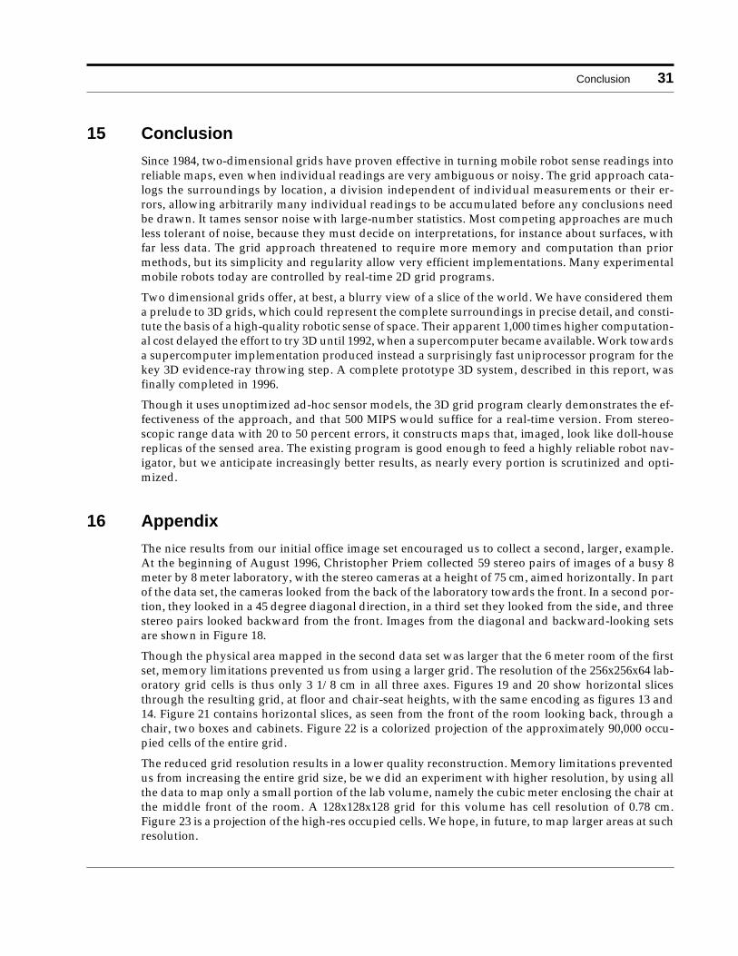
The nice results from our initial office image set encouraged us to collect a second, larger, example.At the beginning of August 1996, Christopher Priem collected 59 stereo pairs of images of a busy 8meter by 8 meter laboratory, with the stereo cameras at a height of 75 cm, aimed horizontally. In partof the data set, the cameras looked from the back of the laboratory towards the front. In a second por-tion, they looked in a 45 degree diagonal direction, in a third set they looked from the side, and threestereo pairs looked backward from the front. Images from the diagonal and backward-looking setsare shown in Figure 18.

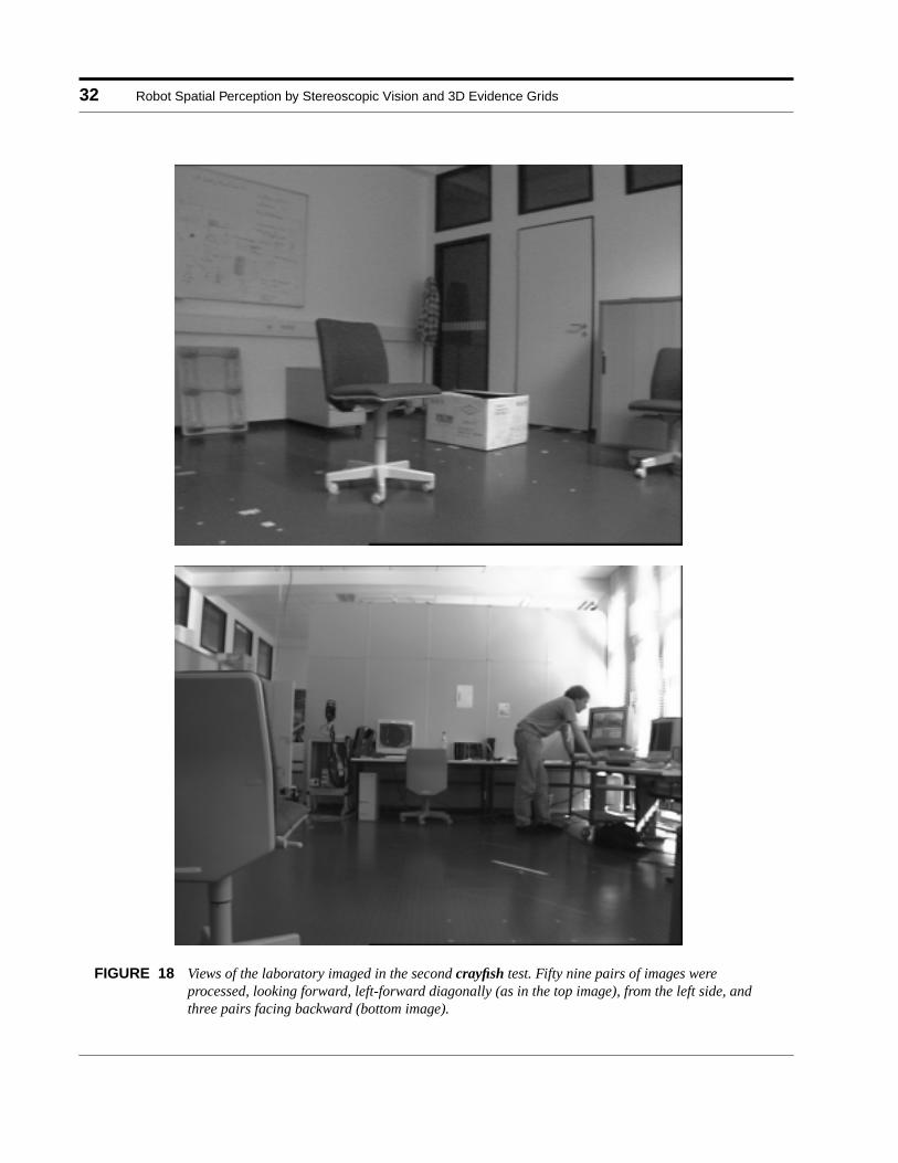
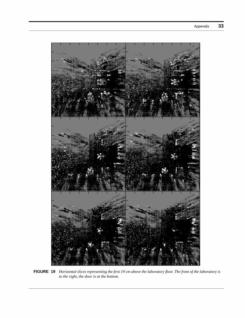
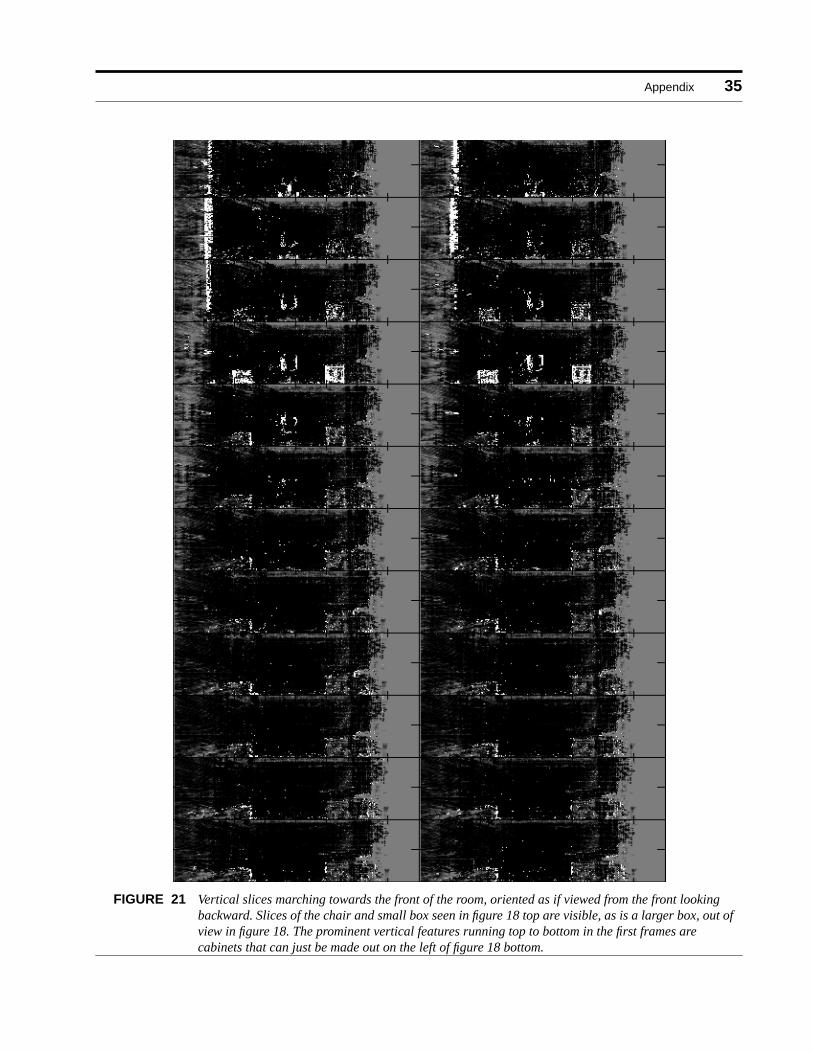
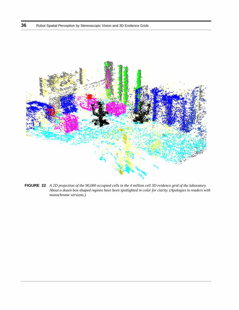
Though the physical area mapped in the second data set was larger that the 6 meter room of the firstset, memory limitations prevented us from using a larger grid. The resolution of the 256x256x64 lab-oratory grid cells is thus only 3 1/8 cm in all three axes. Figures 19 and 20 show horizontal slicesthrough the resulting grid, at floor and chair-seat heights, with the same encoding as figures 13 and14. Figure 21 contains horizontal slices, as seen from the front of the room looking back, through achair, two boxes and cabinets. Figure 22 is a colorized projection of the approximately 90,000 occu-pied cells of the entire grid.

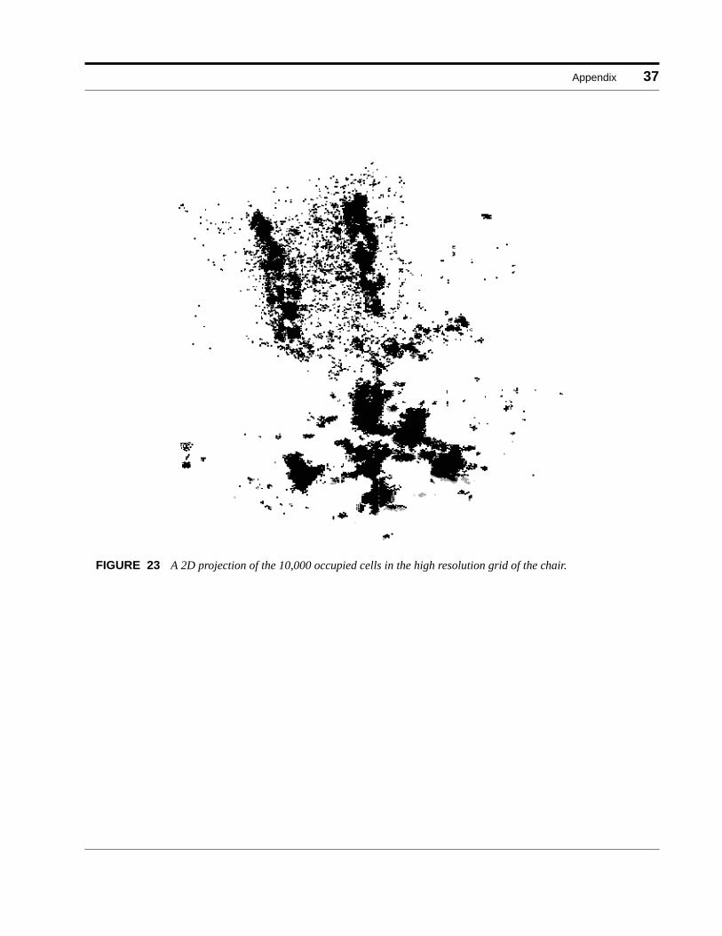
The reduced grid resolution results in a lower quality reconstruction. Memory limitations preventedus from increasing the entire grid size, be we did an experiment with higher resolution, by using allthe data to map only a small portion of the lab volume, namely the cubic meter enclosing the chair atthe middle front of the room. A 128x128x128 grid for this volume has cell resolution of 0.78 cm.Figure 23 is a projection of the high-res occupied cells. We hope, in future, to map larger areas at suchresolution.


FIGURE 18 Views of the laboratory imaged in the second crayfish test. Fifty nine pairs of images wereprocessed, looking forward, left-forward diagonally (as in the top image), from the left side, andthree pairs facing backward (bottom image).

Appendix 33

FIGURE 19 Horizontal slices representing the first 19 cm above the laboratory floor. The front of the laboratory isto the right, the door is at the bottom.


FIGURE 20 Horizontal slices 38 to 56 cm above the laboratory floor.

Appendix 35

FIGURE 21 Vertical slices marching towards the front of the room, oriented as if viewed from the front lookingbackward. Slices of the chair and small box seen in figure 18 top are visible, as is a larger box, out ofview in figure 18. The prominent vertical features running top to bottom in the first frames arecabinets that can just be made out on the left of figure 18 bottom.


FIGURE 22 A 2D projection of the 90,000 occupied cells in the 4 million cell 3D evidence grid of the laboratory.About a dozen box-shaped regions have been spotlighted in color for clarity. (Apologies to readers withmonochrome versions.)

Appendix 37

FIGURE 23 A 2D projection of the 10,000 occupied cells in the high resolution grid of the chair.


17 References

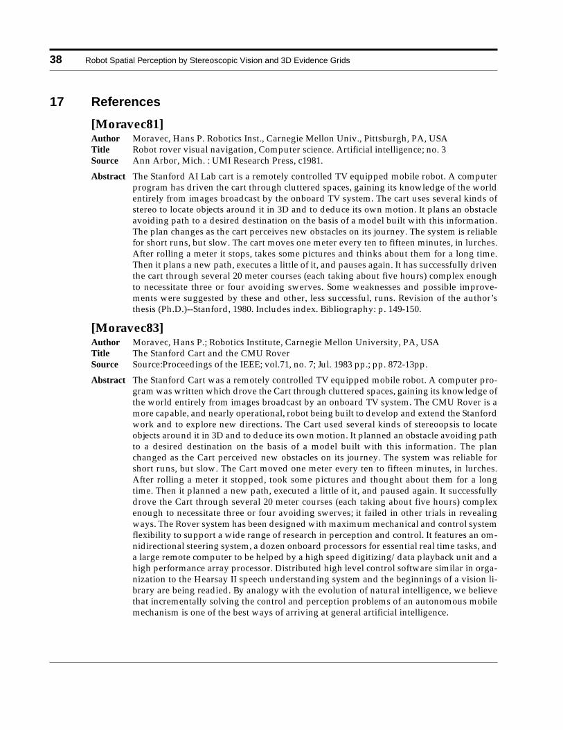
[Moravec81]Author Moravec, Hans P. Robotics Inst., Carnegie Mellon Univ., Pittsburgh, PA, USATitle Robot rover visual navigation, Computer science. Artificial intelligence; no. 3Source Ann Arbor, Mich. : UMI Research Press, c1981.

Abstract The Stanford AI Lab cart is a remotely controlled TV equipped mobile robot. A computerprogram has driven the cart through cluttered spaces, gaining its knowledge of the worldentirely from images broadcast by the onboard TV system. The cart uses several kinds ofstereo to locate objects around it in 3D and to deduce its own motion. It plans an obstacleavoiding path to a desired destination on the basis of a model built with this information.The plan changes as the cart perceives new obstacles on its journey. The system is reliablefor short runs, but slow. The cart moves one meter every ten to fifteen minutes, in lurches.After rolling a meter it stops, takes some pictures and thinks about them for a long time.Then it plans a new path, executes a little of it, and pauses again. It has successfully driventhe cart through several 20 meter courses (each taking about five hours) complex enoughto necessitate three or four avoiding swerves. Some weaknesses and possible improve-ments were suggested by these and other, less successful, runs. Revision of the author’sthesis (Ph.D.)--Stanford, 1980. Includes index. Bibliography: p. 149-150.

[Moravec83]Author Moravec, Hans P.; Robotics Institute, Carnegie Mellon University, PA, USATitle The Stanford Cart and the CMU RoverSource Source:Proceedings of the IEEE; vol.71, no. 7; Jul. 1983 pp.; pp. 872-13pp.

Abstract The Stanford Cart was a remotely controlled TV equipped mobile robot. A computer pro-gram was written which drove the Cart through cluttered spaces, gaining its knowledge ofthe world entirely from images broadcast by an onboard TV system. The CMU Rover is amore capable, and nearly operational, robot being built to develop and extend the Stanfordwork and to explore new directions. The Cart used several kinds of stereoopsis to locateobjects around it in 3D and to deduce its own motion. It planned an obstacle avoiding pathto a desired destination on the basis of a model built with this information. The planchanged as the Cart perceived new obstacles on its journey. The system was reliable forshort runs, but slow. The Cart moved one meter every ten to fifteen minutes, in lurches.After rolling a meter it stopped, took some pictures and thought about them for a longtime. Then it planned a new path, executed a little of it, and paused again. It successfullydrove the Cart through several 20 meter courses (each taking about five hours) complexenough to necessitate three or four avoiding swerves; it failed in other trials in revealingways. The Rover system has been designed with maximum mechanical and control systemflexibility to support a wide range of research in perception and control. It features an om-nidirectional steering system, a dozen onboard processors for essential real time tasks, anda large remote computer to be helped by a high speed digitizing/data playback unit and ahigh performance array processor. Distributed high level control software similar in orga-nization to the Hearsay II speech understanding system and the beginnings of a vision li-brary are being readied. By analogy with the evolution of natural intelligence, we believethat incrementally solving the control and perception problems of an autonomous mobilemechanism is one of the best ways of arriving at general artificial intelligence.

References 39

[Moravec-Elfes85]Author Moravec, H.P.; Elfes, A.E.; Robotics Institute, Carnegie Mellon University, PA, USATitle High Resolution Maps from Wide Angle SonarSource Proceedings of the 1985 IEEE International Conference on Robotics and Automation, St.

Louis, March, 1985, pp 116-121;

Abstract We describe the use of multiple wide-angle sonar range measurements to map the sur-roundings of an autonomous mobile robot. A sonar range reading provides informationconcerning empty and occupied volumes in a cone (subtending 30 deg in our case) in frontof the sensor. The reading is modelled as probability profiles projected onto a rasterizedmap, where somewhere occupied and everywhere empty areas are represented. Rangemeasurements from multiple points of view (taken from multiple sensors on the robot, andfrom the same sensors after robot moves) are systematically integrated in the map. Over-lapping empty volumes re-inforce each other, and serve to condense the range of occupiedvolumes. The map definition improves as more readings are added. The final map showsregions probably occupied, probably unoccupied, and unknown areas. The method dealseffectively with clutter, and can be used for motion planning and for extended landmarkrecognition. This system has been tested on the Neptune mobile robot at CMU.

[Elfes87]Author Elfes, A.; Robotics Inst., Carnegie-Mellon Univ., Pittsburgh, PA, USATitle Sonar-based real-world mapping and navigationSource IEEE Journal of Robotics and Automation; IEEE J. Robot. Autom. (USA); vol.RA-3, no.3;

A07; June 1987 ; pp. 249-65 pp.

Abstract A sonar-based mapping and navigation system developed for an autonomous mobile ro-bot operating in unknown and unstructured environments is described. The system usessonar range data to build a multileveled description of the robot’s surroundings. Sonarreadings are interpreted using probability profiles to determine empty and occupied areas.Range measurements from multiple points of view are integrated into a sensor-level sonarmap, using a robust method that combines the sensor information in such a way as to copewith uncertainties and errors in the data. The sonar mapping procedures have been imple-mented as part of an autonomous mobile robot navigation system called Dolphin. The ma-jor modules of this system are described and related to the various mappingrepresentations used. Results from actual runs are presented, and further research is men-tioned. The system is also situated within the wider context of developing an advancedsoftware architecture for autonomous mobile robots.

[Moravec-Blackwell93]Author Moravec, H.P.; Blackwell, M.; Robotics Inst., Carnegie Mellon Univ., Pittsburgh, PA, USATitle Learning Sensor Models for Evidence GridsSource CMU Robotics Institute 1991 Annual Research Review, 1993, pp.8-15.

Abstract Evidence grids (aka. occupancy, probability and certainty grids) are a probabilistic, finite-element representation of robot spatial knowledge. The grids allow the efficient accumula-tion of small amounts of information from individual sensor readings into increasingly ac-curate and confident maps. Each sensor measurement is translated, via a sensor model,into a spatial evidence distribution that is added to a grid representing the robot’s sur-roundings. In our first applications of the method, on a mobile robot with a ring of 24 Po-laroid sonar transducers autonomously navigating a cluttered room, we constructed thesensor model from a cursory examination of the Polaroid literature. Despite the ad-hoc


model, the grid approach worked far better than an older program, a decade in develop-ment, that used a geometric model. It successfully navigated cluttered rooms, most hall-ways, a coal mine and outdoors. The original program failed in a smooth-walled narrowcorridor, where most sonar pulses, deflected by mirrorlike walls, indicated overlong rang-es. The evidence grid method might be able to slowly accumulate evidence from such data,if only the sensor model accurately represented the modest information contained in areading, as our ad-hoc model did not. This paper reports on a learning program that findsgood models automatically. The sensor model is formulated as a closed form expressionshaped by several parameters. The parameters are adjusted, in a hill-climbing process, thatmaximizes the match between a hand-constructed ideal map and a map built by the modelwith data from a robot test run in the mapped area. Using this approach with a 9- param-eter function a program using several weeks of Sparc1+ workstation search time was ableto produce a crisp, correct map of the difficult smooth hallway, from data that produces anunrecognizable splatter when interpreted by our original ad-hoc sensor model.

[Hellwich&al94]Author Hellwich, O.; Heipke, C.; Liang Tang; Ebner, H.; Mayr, W.; Tech. U. Munchen, GermanyTitle Experiences with automatic relative orientationSource ISPRS Commission III Symposium Spatial Information from Digital Photogrammetry and

Computer Vision; Munich, Germany; 5-9 Sept. 199 Sponsored by: SPIE; Proceedings of theSPIE - The International Society for Optical Engineering; Proc. SPIE - Int. Soc. Opt. Eng.(USA); vol.2357, pt.1; 1994; pp. 370-8

Abstract A report on recent experiences with a new procedure for automatic relative orientation isgiven. A hierarchical approach provides conjugate points using image pyramids. The im-plemented method is based on feature extraction by an interest operator, feature matchingbetween the two images, area based image correlation, a robust least squares bundle ad-justment and feature tracking through several levels of the image pyramid. The automaticprocedure proved to be successful for various combinations of terrain relief surface coverand image scale. The paper presents the results of intensive tests. It was found that only alimited number of control parameters of the algorithm has to be individually adjusted tothe terrain specifics. Further investigations need to be conducted to find out whether theproject dependent parameters can be reliably predicted for certain classes of images.

[Stunz-Knopfle-Roth94]Author Strunz, G.; Knopfle, W.; Roth, A.; Remote Sensing Data Centre, German Aerosp. Res. Es-

tabl., Oberpfaffenhofen, GermanyTitle Automation of tie pointing procedure for the geocoding of satellite imagesSource ISPRS Commission III Symposium Spatial Information from Digital Photogrammetry and

Computer Vision; Munich, Germany; 5-9 Sept. 1994, SPIE; Proceedings of the SPIE - The In-ternational Society for Optical Engineering; Proc. SPIE - Int. Soc. Opt. Eng. (USA); vol.2357,pt.2; 1994; pp. 793-800

Abstract The comprehensive utilization of the information content provided by remote sensing sat-ellites requires the multitemporal and multisensoral analysis of the image data. Prior tothis analysis, processing is necessary to correct for geometric distortions. To handle thelarge amount of data and the high data rates, the traditional approach of visual identifica-tion of control or tie points is not an acceptable solution. The paper describes two develop-ments at the German Remote Sensing Data Centre, which aim at the automatic generationof tie points for optical sensors and radar images, and the operational utilization of auto-matic tie pointing for ERS-1 SAR data. A concept for the multitemporal registration of sat-

References 41

ellite images from optical sensors is described. This approach comprises the detection ofdistinct points by a so-called interest operator in one image. By cross correlation, the cor-responding points in the other images are traced. Subpixel accuracy is achieved by a leastsquares technique for digital image matching. Practical results are shown, where multitem-poral image data from the Landsat TM sensor are used. The paper also describes the oper-ational utilization of an automatic tie pointing which has been realized for the geocodingof the ERS-1 SAR data at the German Processing and Archiving Facility. Significant fea-tures are extracted from reference data sets. The procedure is described as well as the ac-curacy achieved. An outlook is given concerning several automatic approaches beinginvestigated.

[Koenig-Simmons96]Author Koenig, S.; Simmons, R.G.; Sch. of Comp. Sci., Carnegie Mellon Univ., Pittsburgh, PA, USATitle Unsupervised learning of probabilistic models for robot navigationSource Proceedings of IEEE International Conference on Robotics and Automation; Part: vol.3;

Minneapolis, MN, USA; 22-28 April 1996; sponsored by: IEEE Robotics & Autom. Soc; Pro-ceedings. 1996 IEEE International Conference on Robotics and Automation (Cat. No.96CH35857); New York, NY, USA; IEEE; 4 vol. lxiv+3749; 1996; pp. 2301-8 vol.3

Abstract Navigation methods for office delivery robots need to take various sources of uncertaintyinto account in order to get robust performance. In previous work, we developed a reliablenavigation technique that uses partially observable Markov models to represent metric, ac-tuator and sensor uncertainties. This paper describes an algorithm that adjusts the proba-bilities of the initial Markov model by passively observing the robot’s interactions with itsenvironment. The learned probabilities more accurately reflect the actual uncertainties inthe environment, which ultimately leads to improved navigation performance. The algo-rithm, an extension of the Baum-Welch algorithm, learns without a teacher and addressesthe issues of limited memory and the cost of collecting training data. Empirical resultsshow that the algorithm learns good Markov models with a small amount of training data.

[Yamauchi96]Author Yamauchi, B.; Inst. for the Study of Learning & Experience, Palo Alto, CA, USATitle Mobile robot localization in dynamic environments using dead reckoning and evidence

gridsSource Proceedings of IEEE International Conference on Robotics and Automation; Part: vol.2;

Minneapolis, MN, USA; 22-28 April 1996; Sponsored by: IEEE Robotics & Autom. Soc;Proceedings. 1996 IEEE International Conference on Robotics and Automation (Cat. No.96CH35857); New York, NY, USA; IEEE; 4 vol. lxiv+3749; 1996; pp. 1401-6 vol.2

Abstract Dead reckoning provides a simple way to keep track of a mobile robot’s location. However,due to slippage between the robot’s wheels and the underlying surface, this position esti-mate accumulates errors over time. In this paper, we introduce a method for correctingdead reckoning errors by matching evidence grids constructed at different times. A hill-climbing algorithm is used to search the space of possible translations and rotations usedto transform one grid into the other. The transformation resulting in the best match is usedto correct the robot’s position estimate. This technique has been tested on a real mobile ro-bot and has demonstrated robustness to transient changes (moving people) and lastingchanges (rearranged obstacles) in dynamic environments.


[Schultz-Adams-Grefenstette96]Author Alan C. Schultz, William Adams, and John J. Grefenstette (1996). NCARAI,Naval Research

Laboratory, Washington, DC 20375-5337Title Continuous localization using evidence gridsSource NCARAI Report AIC-96-007, Naval Research Laboratory, Washington, DC.

[email protected]

Abstract The evidence grid representation provides a uniform representation for fusing temporallyand spatially distinct sensor readings. However, the use of evidence grids requires that therobot be localized within its environment. Odometry errors typically accumulate overtime, making localization estimates degrade, and introducing significant errors into evi-dence grids as they are built. We have addressed this problem by developing a new meth-od for ``continuous localization’’, in which the robot corrects its localization estimatesincrementally and on the fly. Assuming the mobile robot has a map of its environment rep-resented as an evidence grid, localization is achieved by building a series of ``local percep-tion grids,’’ also represented as evidence grids, based on localized sensor readings and thecurrent odometry, and then registering the local and global grids. The registration produc-es an offset which is used to correct the odometry. Results are given on the effectiveness ofthis method, and quantify the improvement of continuous localization over dead reckon-ing. Further results show that maps built of the room using evidence grids while the robotis performing continuous localization show no appreciable systematic errors due to odo-metric error; it appears that maps of the room can simultaneously be learned and used forcontinous localization.

[Martin-Moravec96]Author Author:Martin, M.C.; Moravec, H.P.; Robotics Inst., Carnegie Mellon Univ., Pittsburgh,

PA, USATitle Robot Evidence GridsSource Carnegie Mellon University, Robotics Institute Technical Report CMU-RI-TR-96-06

Abstract The evidence grid representation was formulated at the CMU Mobile Robot Laboratory in1983 to turn wide angle range measurements from cheap mobile robot-mounted sonar sen-sors into detailed spatial maps. Whereas most older approaches to mapping considered thelocation of objects, the grid approach weighs the “objectness” of locations. It accumulatesdiffuse evidence about the occupancy of a grid of small volumes of nearby space from in-dividual sensor readings into increasingly confident and detailed maps of a robot’s sur-roundings. It worked surprisingly well in first implementation for sonar navigation incluttered rooms. In the past decade its use has been extended to range measurements fromstereoscopic vision and other sensors, sonar in very difficult specular environments, andother contexts. The most dramatic extension yet, from 2D grid maps with thousands ofcells to 3D grids with millions, is underway. This paper presents the mathematical andprobabilistic framework we now use for evidence grids. It gives the history of the grid rep-resentation, and its relation to other spatial modeling approaches. It discusses earlier for-mulations and their limitations, and documents several extensions. A list of open issuesand research topics is then presented, followed by a literature survey.

Robot Spatial Perception Stereoscopic Vision 3D...

Documents

Transcript of Robot Spatial Perception Stereoscopic Vision 3D...