Robot Dynamics – Newton- Euler Recursive Approach

ME 4135 Robotics & Controls

R. Lindeke, Ph. D.

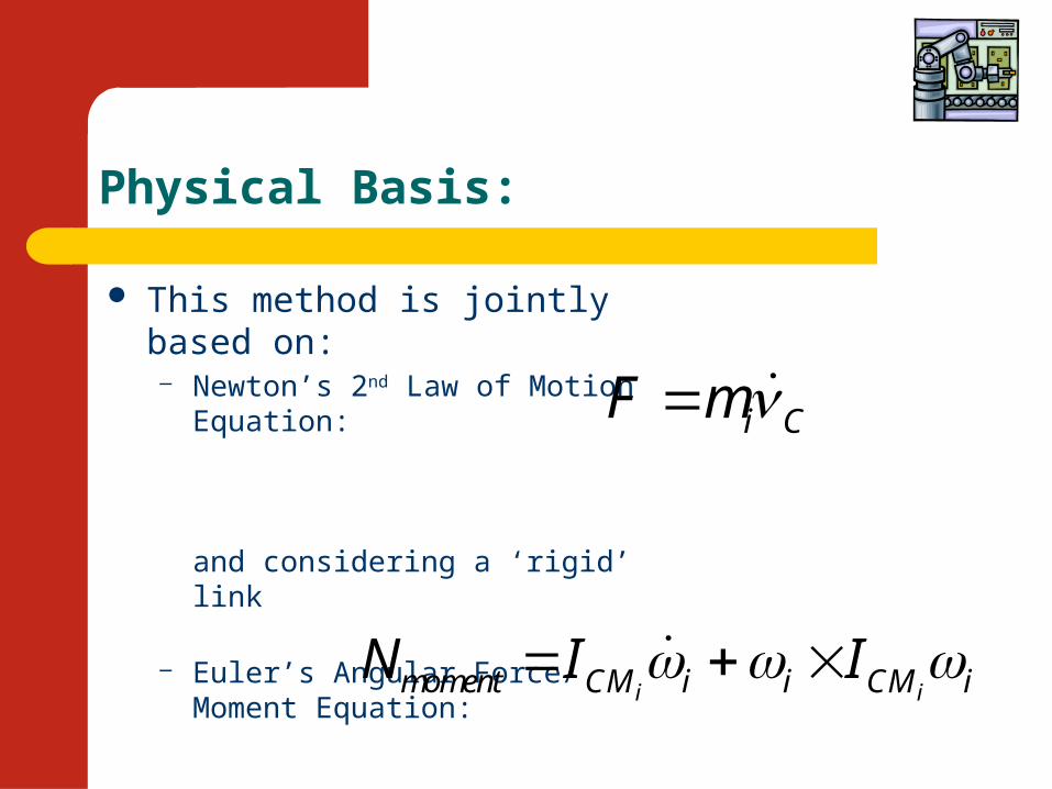
Physical Basis:

This method is jointly based on:– Newton’s 2nd Law of Motion

Equation:

and considering a ‘rigid’ link

– Euler’s Angular Force/ Moment Equation:

i CF m

i imoment CM i i CM iN I I

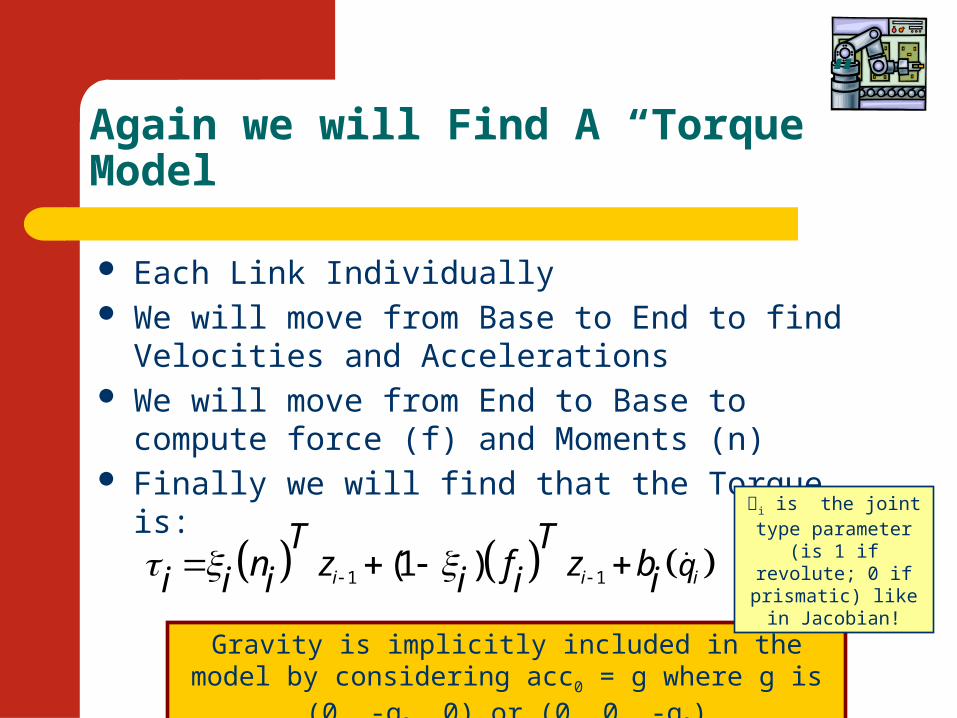
Again we will Find A “Torque” Model

Each Link Individually We will move from Base to End to find Velocities

and Accelerations We will move from End to Base to compute force

(f) and Moments (n) Finally we will find that the Torque is:

1 1(1 )i i iqT T

n z f z bi i i i i i

Gravity is implicitly included in the model by considering acc0 = g where g is (0, -g0, 0) or (0, 0, -g0)

i is the joint type parameter (is 1 if

revolute; 0 if prismatic) like in

Jacobian!

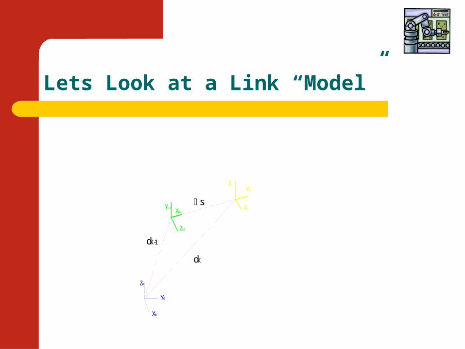
Lets Look at a Link “Model”

X0

Y0

Z0

Zk-1

Xk-1Yk-1

ZK

XK

YK

dK

dK-1

sK

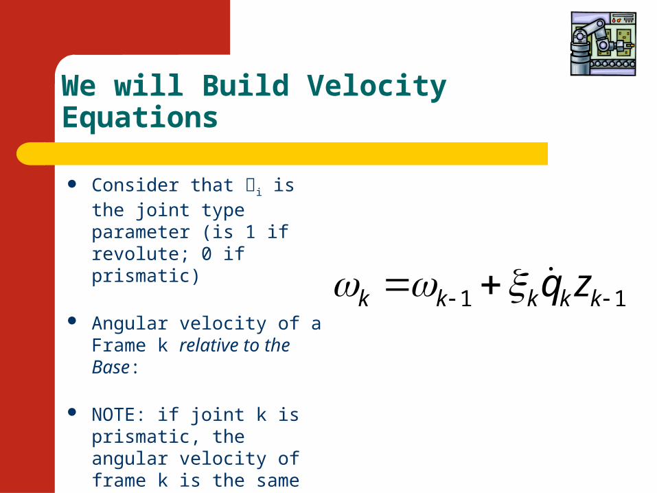
We will Build Velocity Equations

Consider that i is the joint type parameter (is 1 if revolute; 0 if prismatic)

Angular velocity of a Frame k relative to the Base:

NOTE: if joint k is prismatic, the angular velocity of frame k is the same as angular velocity of frame k-1!

1 1k k k k kq z

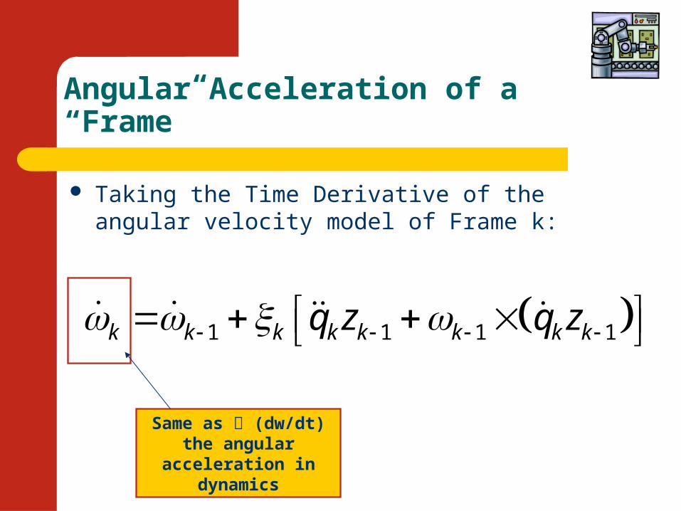
Angular Acceleration of a “Frame”

Taking the Time Derivative of the angular velocity model of Frame k:

1 1 1 1k k k k k k k kq z q z

Same as (dw/dt) the angular acceleration in

dynamics

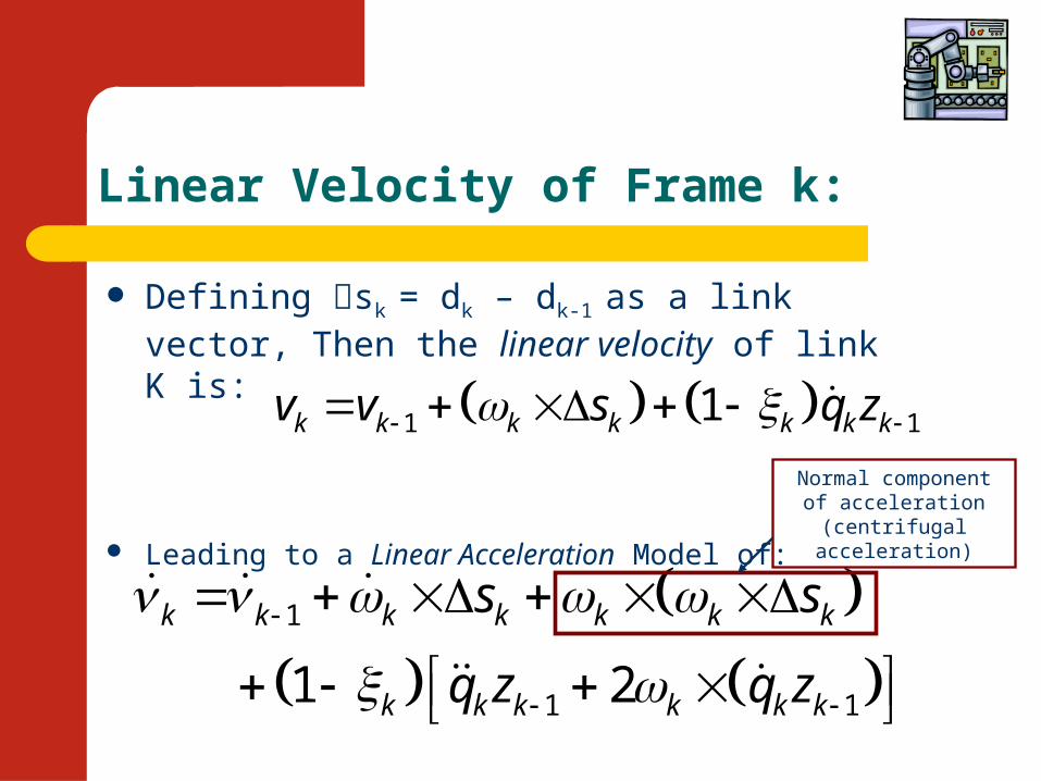
Linear Velocity of Frame k:

Defining sk = dk – dk-1 as a link vector, Then the linear velocity of link K is:

Leading to a Linear Acceleration Model of:

1 11k k k k k k kv v s q z

1

1 11 2

k k k k k k k

k k k k k k

s s

q z q z

Normal component of acceleration (centrifugal

acceleration)

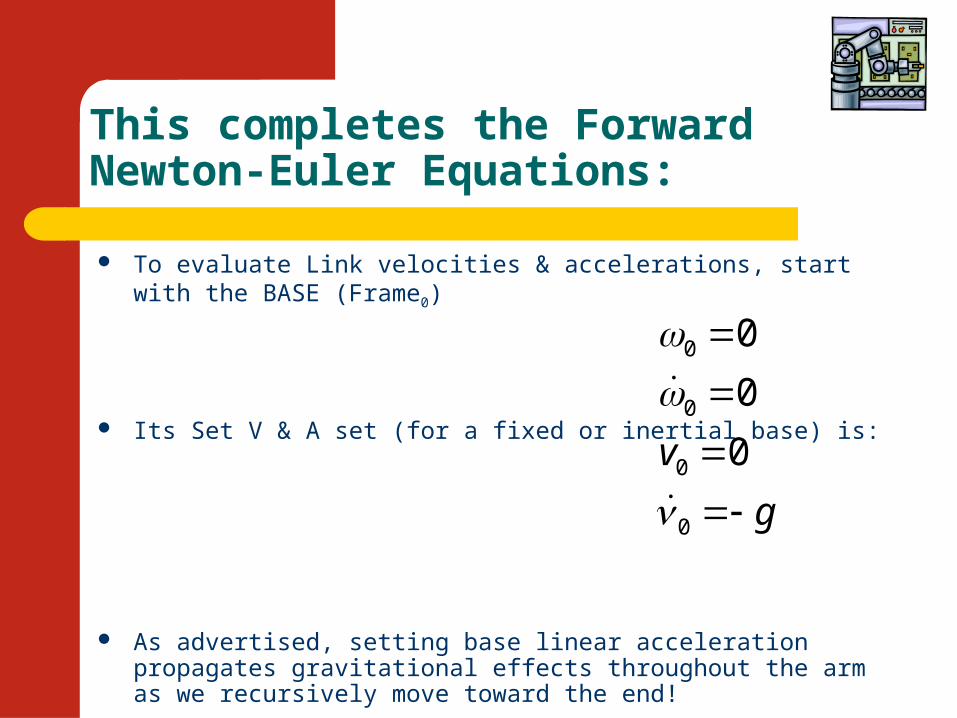
This completes the Forward Newton-Euler Equations:

To evaluate Link velocities & accelerations, start with the BASE (Frame0)

Its Set V & A set (for a fixed or inertial base) is:

As advertised, setting base linear acceleration propagates gravitational effects throughout the arm as we recursively move toward the end!

0

0

0

0

0

0

0v

g

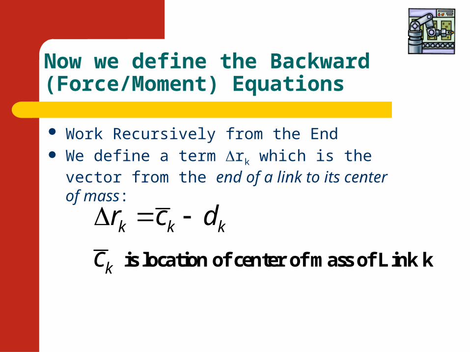
Now we define the Backward (Force/Moment) Equations

Work Recursively from the End We define a term rk which is the vector from

the end of a link to its center of mass:

k k k

k

r c d

c

is location of center of mass of Link k

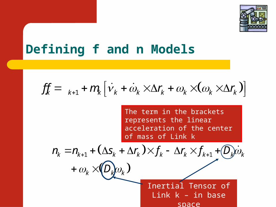
Defining f and n Models

1k k k k k k k k kf f m r r

1 1k k k k k k k k k

k k k

n n s r f r f D

D

Inertial Tensor of Link k – in base space

The term in the brackets represents the linear acceleration of the center of mass of Link k

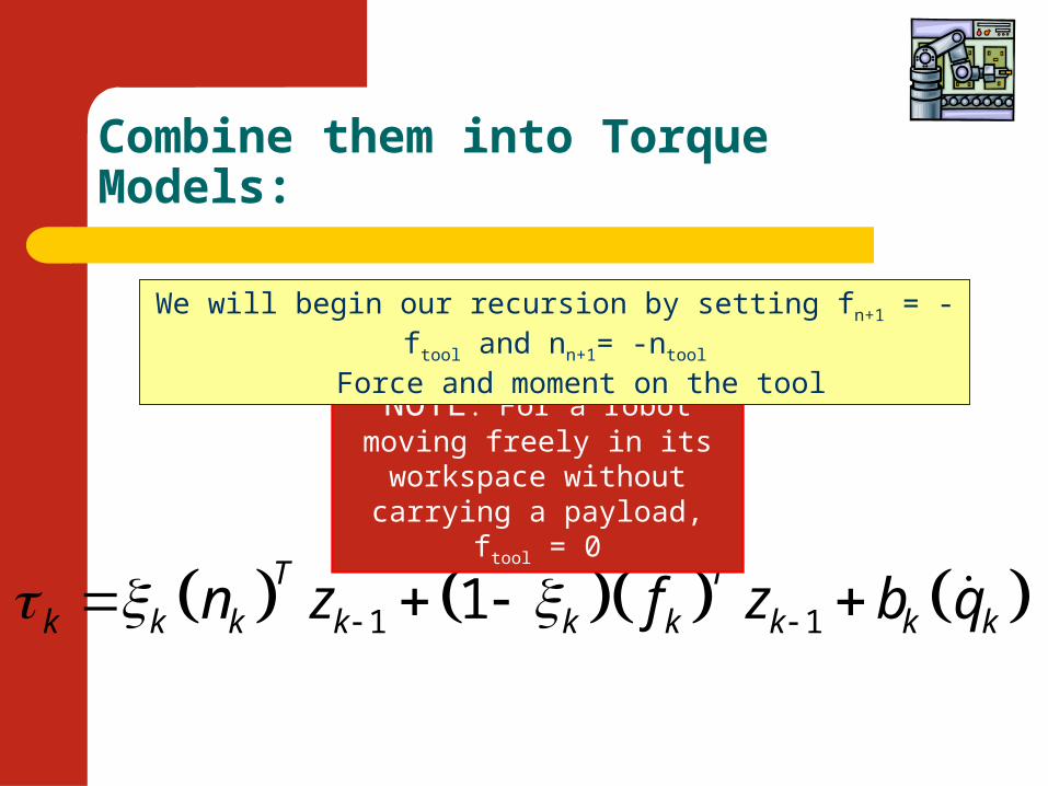
Combine them into Torque Models:

1 11T T

k k k k k k k k kn z f z b q

NOTE: For a robot moving freely in its workspace without

carrying a payload, ftool = 0

We will begin our recursion by setting fn+1 = -ftool and nn+1= -ntool

Force and moment on the tool

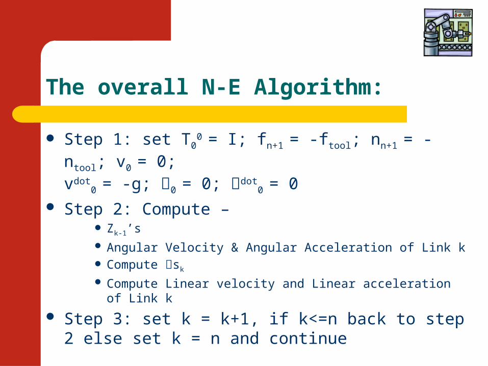
The overall N-E Algorithm:

Step 1: set T00 = I; fn+1 = -ftool; nn+1 = -ntool; v0 = 0;

vdot0 = -g; 0 = 0; dot

0 = 0 Step 2: Compute –

Zk-1’s Angular Velocity & Angular Acceleration of Link k Compute sk

Compute Linear velocity and Linear acceleration of Link k

Step 3: set k = k+1, if k<=n back to step 2 else set k = n and continue

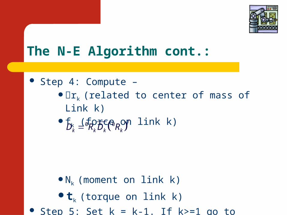
The N-E Algorithm cont.:

Step 4: Compute – rk (related to center of mass of Link k)

fk (force on link k)

Nk (moment on link k)

tk (torque on link k) Step 5: Set k = k-1. If k>=1 go to step 4

0 0 T

k k k kD R D R

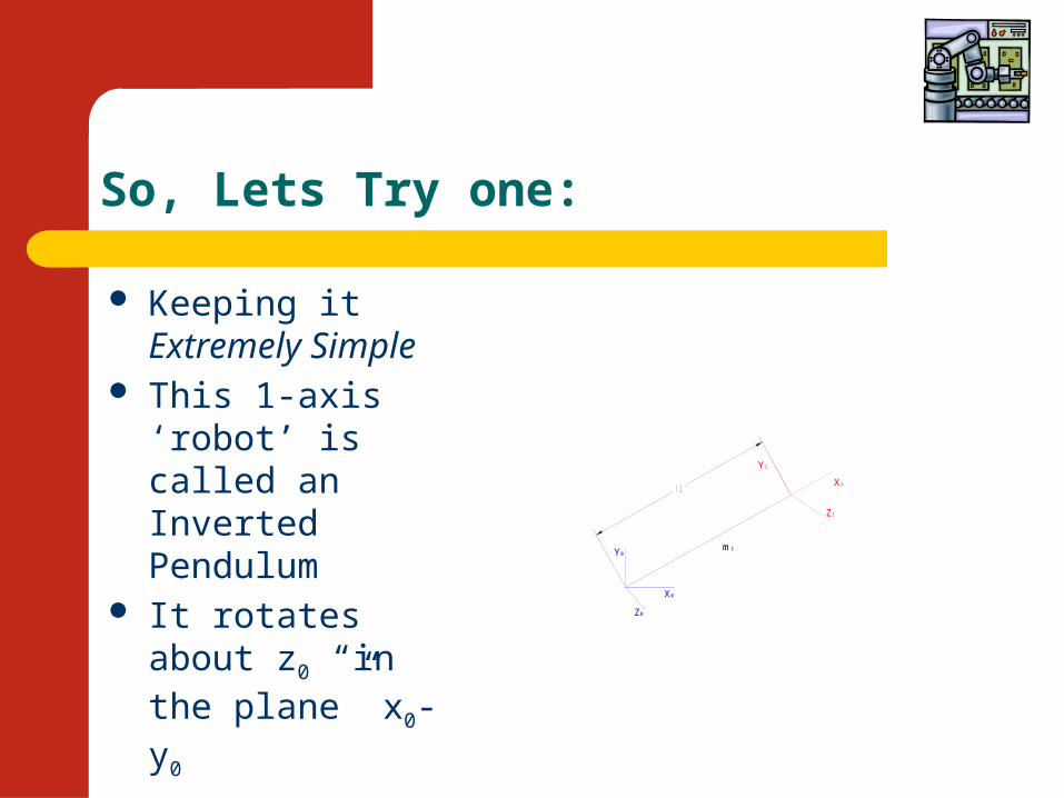
So, Lets Try one:

Keeping it Extremely Simple

This 1-axis ‘robot’ is called an Inverted Pendulum

It rotates about z0 “in the plane” x0-y0 X0

Z0

Y0m1

Y1

X1

Z1

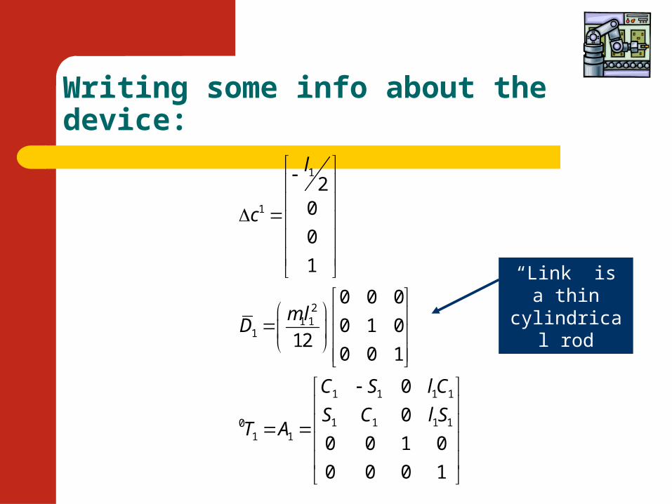
Writing some info about the device:

1

1

21 1

1

1 1 1 1

1 1 1 101 1

20

0

1

0 0 0

0 1 012

0 0 1

0

0

0 0 1 0

0 0 0 1

l

c

m lD

C S l C

S C l ST A

“Link” is a thin cylindrical rod

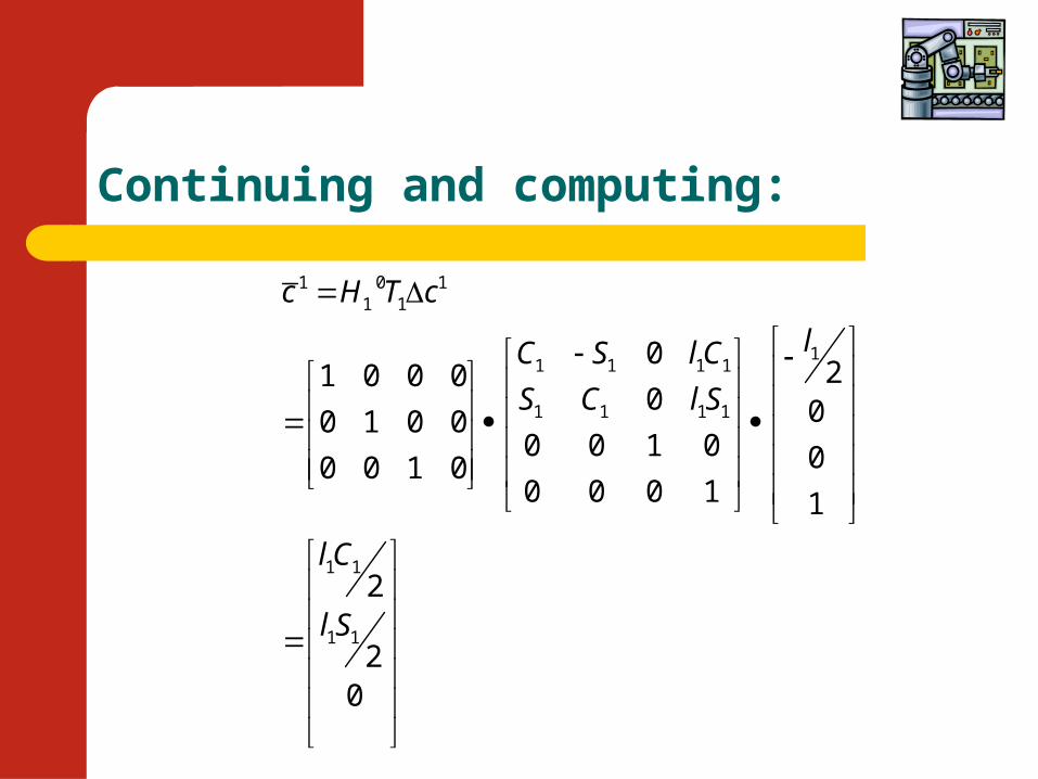
Continuing and computing:

1 0 11 1

11 1 1 1

1 1 1 1

1 1

1 1

021 0 0 0

0 00 1 0 00 0 1 0 00 0 1 00 0 0 1 1

2

20

c H T c

lC S l C

S C l S

l C

l S

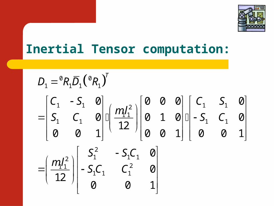
Inertial Tensor computation:

0 01 1 1 1

1 1 1 121 1

1 1 1 1

21 1 12

21 11 1 1

0 0 0 0 0

0 0 1 0 012

0 0 1 0 0 1 0 0 1

0

012

0 0 1

TD R D R

C S C Sm l

S C S C

S S Cm l

S C C

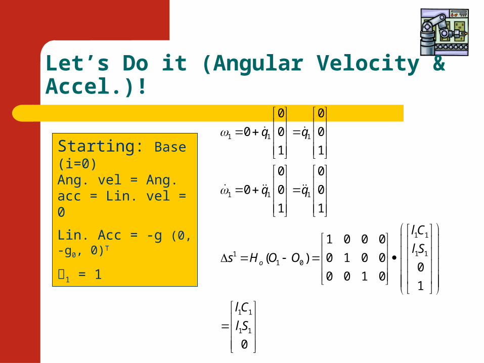
Let’s Do it (Angular Velocity & Accel.)!

1 1 1

1 1 1

1 1

1 111 0

1 1

1 1

0 0

0 0 0

1 1

0 0

0 0 0

1 1

1 0 0 0

( ) 0 1 0 00

0 0 1 01

0

o

q q

q q

l C

l Ss H O O

l C

l S

Starting: Base (i=0)Ang. vel = Ang. acc = Lin. vel = 0

Lin. Acc = -g (0, -g0, 0)T

1 = 1

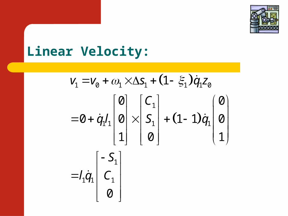
Linear Velocity:

1 0 1 1 1 1 0

1

1 1 1 1

1

1 1 1

1

0 0

0 0 1 1 0

1 0 1

0

v v s q z

C

q l S q

S

l q C

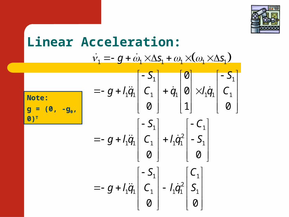
Linear Acceleration: 1 1 1 1 1 1

1 1

1 1 1 1 1 1 1

1 12

1 1 1 1 1 1

1 12

1 1 1 1 1 1

0

0

0 1 0

0 0

0 0

g s s

S S

g l q C q l q C

S C

g l q C l q S

S C

g l q C l q S

Note:

g = (0, -g0, 0)T

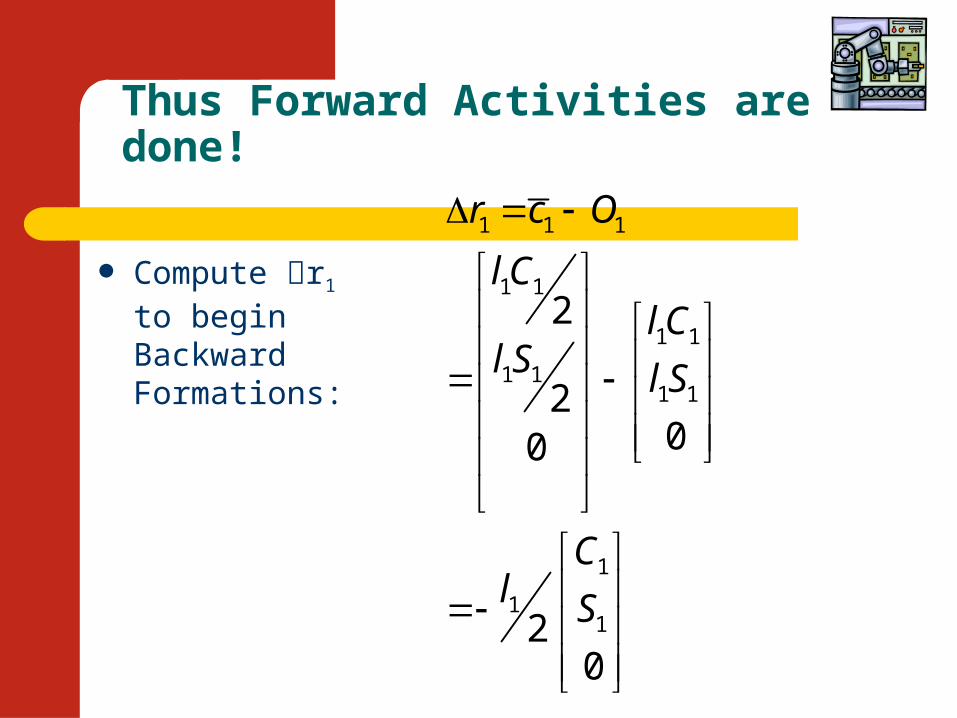
Thus Forward Activities are done!

Compute r1 to begin Backward Formations:

1 1 1

1 1

1 1

1 11 1

1

11

2

200

20

r c O

l Cl C

l S l S

Cl S

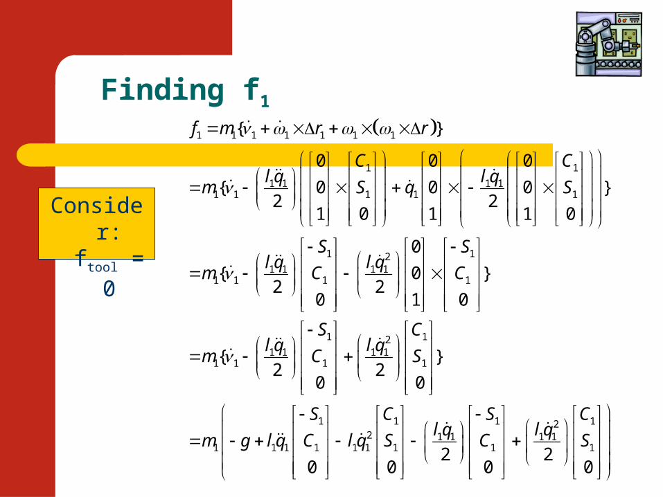
Finding f1

Consider: ftool = 0

1 1 1 1 1 1 1

1 1

1 1 1 11 1 1 1 1

1

1 11 1 1

{ }

0 0 0

{ 0 0 0 }2 2

1 0 1 1 0

{2

0

f m r r

C Cl q l q

m S q S

Sl q

m C

12

1 11

1 121 1 1 1

1 1 1 1

1 1 1 22 1 1 1 1

1 1 1 1 1 1 1 1

0

0 }2

1 0

{ }2 2

0 0

2 20 0 0

Sl q

C

S Cl q l q

m C S

S C Sl q l q

m g l q C l q S C

1

1

0

C

S

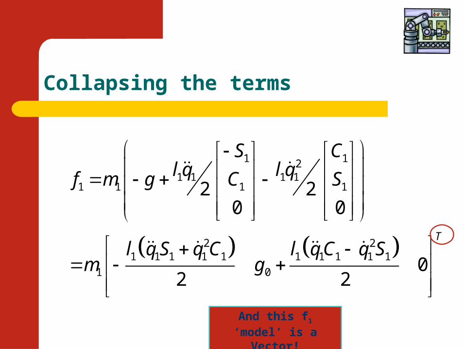
Collapsing the terms

1 121 1 1 1

1 1 1 1

2 21 1 1 1 1 1 1 1 1 1

1 0

2 20 0

02 2

T

S Cl q l qf m g C S

l q S q C l q C q Sm g

And this f1 ‘model’ is a Vector!

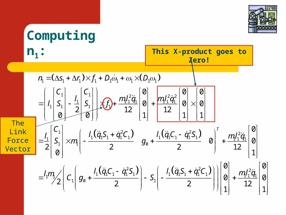
Computing n1:

1 1 1 1 1 1 1 1 1

1 1 2 2 21 1 1 1 1 1 1

1 1 1 1

2 211 1 1 1 1 1 1 1 1 11

1 1 0

0 0 0

0 0 02 12 12

0 0 1 1 1

02 2 20

n s r f D D

C Cl m l q m l q

l S S f

Cl q S q C l q C q Sl

S m g

21 1 1

2 2 21 1 1 1 1 1 1 1 1 1 1 1 11 1

1 0 1

0

012

1

0 0

0 02 2 2 121 1

T

m l q

l q C q S l q S q C m l ql m C g S

This X-product goes to Zero!

The Link Force Vector

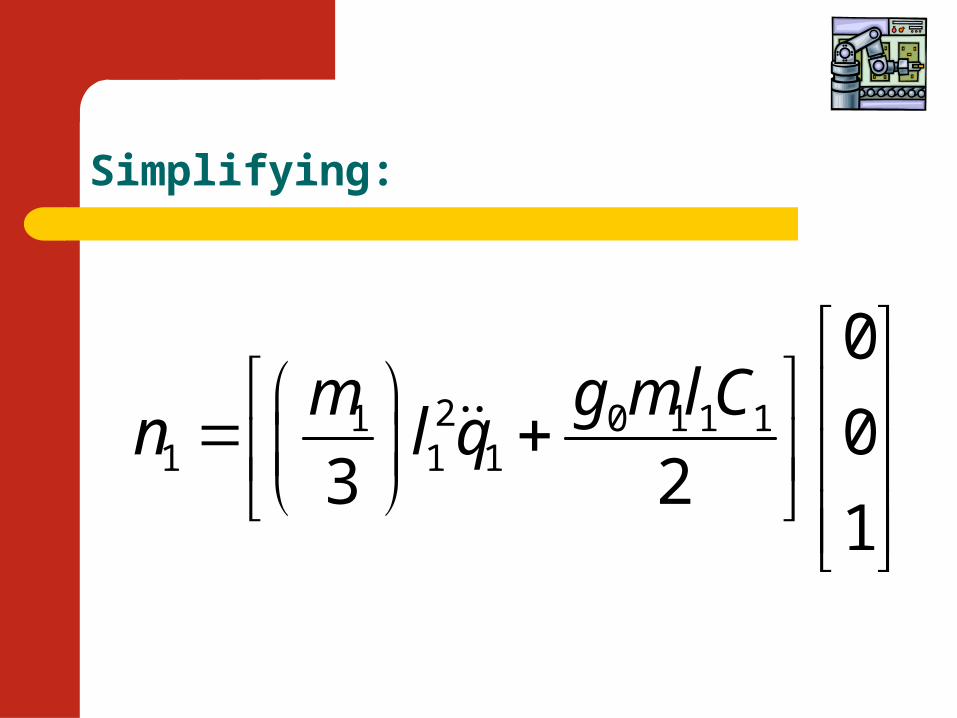
Simplifying:

21 0 1 1 11 1 1

0

03 2

1

m g m l Cn l q

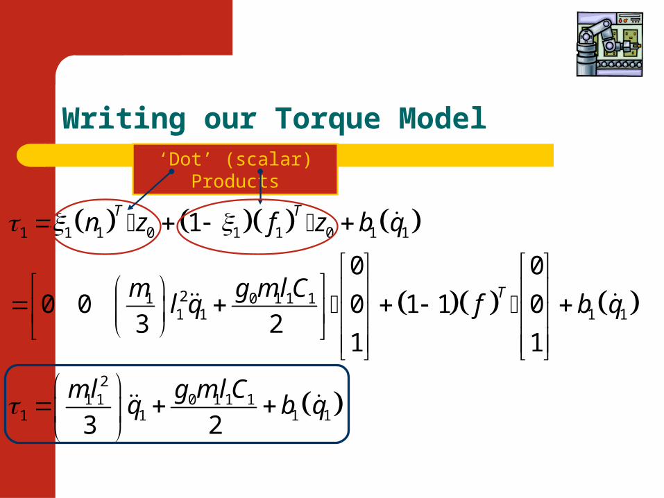
Writing our Torque Model

1 1 1 0 1 1 0 1 1

21 0 1 1 11 1 1 1

21 1 0 1 1 1

1 1 1 1

1

0 0

0 0 0 1 1 03 2

1 1

3 2

T T

T

n z f z b q

m g m l Cl q f b q

m l g m l Cq b q

‘Dot’ (scalar) Products

Homework Assignment (mostly for practice!):

• Compute L-E solution for “Inverted Pendulum & Compare torque model to N-E solution – do and submit by Monday, no better yet --Tuesday!)

• Compute N-E solution for 2 link articulator (of slide set: Dynamics, part 2) and compare to our L-E torque model solution computed there

• Consider Our 4 axis SCARA robot – if the links can be simplified to thin cylinders, develop a generalized torque model for the device.