1

Robert Luther

Aus dem Gebiet der Farbreizmetrik (On color stimulus metrics) Zeitschrift für technische Physik 8 (1927) 540-558 An English translation with a short biographical introduction by Rolf G. Kuehni and a technical introduction by Michael H. Brill Copyright statement: Copyright of original paper: unknown; copyright of translation and biographical introduction: Rolf G. Kuehni, 2009; copyright of technical introduction: Michael H. Brill, 2010

2

Note

Explanatory wording by the translator in angular parentheses. There are three extended

explanatory notes by the translator identified with alphabetical superscripts.

3

Robert Luther 1868-1945

Dresden, ca. 1925 - U. Richter

Robert (Thomas Diedrich) Luther was born in Moscow to German parents on Jan. 2,

1868. His father Alexander was a lawyer. Among his direct ancestors was Hans Luther

(1492-1558), a cousin of the reformer Martin Luther. From 1885 to 1889 he studied

chemistry at the University of Dorpat in Russia. Toward the end of 1889 he was named

assistant to the chemist F. K. Beilstein at the University of St. Petersburg. A serious

illness in 1891 forced him to recuperate during the next two years. In 1894 he resumed

studying chemistry, this time at the University of Leipzig where he received his PhD

degree in 1885. His primary educator there was Wilhelm Ostwald (1853-1931). In 1896

Luther was named an assistant to Ostwald at the Physico-Chemical Institute of the

University of Leipzig. In 1899 Luther submitted his habilitation thesis, titled

“Equilibrium change between halogen compounds of silver and the free halogens caused

by light,” and obtained lecturer status. In the same year he published the monograph “The

chemical processes of photography,” a record of six public lectures he gave on the

subject. In these lectures he demonstrated, among many other things, the chemical

reaction kinetics in layers or volumes of substances, a subject that occupied him for the

rest of his life. He also was the co-author of the 1902 second edition of Ostwald‟s book

on experimental methodology in physico-chemical measurements. In the year 1900 he

was named assistant director of the Ostwald Institute at the University of Leipzig.

As colleagues, Ostwald and Luther were considerably different types. Ostwald did

not like to have to lecture but published many papers and books. As a result, Luther was

burdened with much of the lecturing activities at Ostwald‟s institute. Despite important

work in many fields he rarely wrote articles. In 1904 Luther was named a regular

professor of physical chemistry at the University of Leipzig. Ostwald, wanting to just

manage the Institute, was found to be neglecting his lecturing duties and resigned from

his position in 1906, retreating to his country estate in Grossbothen, where he launched

4

into his color research. In the same year Luther was named director of the newly-formed

photochemical department. In the fall-out of Ostwald‟s departure Luther found himself in

a difficult position in Leipzig and in 1908 accepted an appointment at the Photographic

Science Institute of the Technical University of Dresden, organized shortly before with

the support of the local photographic industry (such as Zeiss). Luther remained there until

his change to professor emeritus status in 1936, performing significant research in

photographic and general physical chemistry and also concerning himself with the

definition of color stimuli and color stimulus measurement. He was much admired by his

students, among them Manfred Richter who later developed the DIN color order system.

In 1909-1910 the famous American photographer Imogen Cunningham (1883-1976) was

a student of Luther, learning the technique of platinum prints. Luther remained in

Dresden where he passed away on April 17, 1945, the last day of the Allied bombing runs

on that city.

Luther‟s interest in color phenomena was the natural outcome of his activities

related to the chemistry of color photography. He clearly distinguished between what he

considered to be objective definition of color stimuli and perceptual color phenomena.

Most of his seminal paper “On color stimulus metrics,” offered here in translation, was

ready for publication in 1923 under the title “Color and spectrum,” as a contribution to a

Festschrift for Ostwald in the Zeitschrift für angewandte Chemie. However, the rabid

inflation of the time prevented publication until 1927, as described in Footnote 4 of the

paper. His only other brief (2 pages) publication on the subject of color, from 1942, is

concerned with practical application of the moment sum curve, developed in the 1927

paper.

Sources of biographical information:

1. M. Richter, Robert Luther, Die Farbe 3:133-135 (1955).

2. A. Fischer, Luther, Robert, in: W. Pötsch (ed.) Lexikon bedeutender Chemiker,

Frankfurt: Verlag Harry Deutsch, 1989.

5

Technical Introduction

The article translated here is a rare summary of thoughts on color by Robert Luther. The

content is quite heterogeneous, because it represents an accumulation of ideas that could

not find earlier publication during a period when Luther‟s Germany faced financial

calamity.

1. General Outline

The article has two main parts. The first part (Sections 1-19), written with the goal of

much earlier publication, is mainly theoretical. In it we find an introduction to tristimulus

space, the embedding therein of the object-color solid (given a pre-defined illuminant

spectrum), and the optimal colors on the exterior surface of the object-color solid

(comprising reflectances that at all visible wavelengths have values of either 0 or 1 with

at most two transitions between them). Some of the optimal colors, called end colors, are

those with only one transition. (Visualizing the optimal-color surface as a clamshell, the

end colors are where the two halves of the shell join.) Other optimal colors, called full

colors, comprise the curve on the object-color solid that would just touch the minimum

cylinder that contains that solid and is parallel to the achromatic axis. (If the object-color

solid were a key and the cylinder were a lock, the full colors would be the points on the

key that brush the inside of the lock.) All these constructs, and others in Luther‟s article,

emerge most immediately from the theoretical work of Wilhelm Ostwald, and also owe

some debt to works such as those of Erwin Schrödinger and Hermann Helmholtz. But

Luther offers some new contributions as well. For example, he was probably the first to

draw the shape of the object-color solid, and did so in several coordinate systems.

The second part (Sections 20-25) is a smorgasbord of material with a more practical

flavor. In Section 20 we find a design of a template colorimeter and a discussion of filter

colorimeters. Section 21 discusses a single-color sensor whose spectral sensitivity is

compensated to the human luminosity sensitivity---a one-dimensional form of a

tristimulus colorimeter or colorimetrically correct camera. Section 22 explains and

endorses heterochromatic flicker photometry. Then Section 23 describes criteria for a

trichromatic camera. Finally, Sections 24 and 25 wax philosophical about subjective

versus objective colors: Luther saw subjective colors as illusions or perturbations on

“real” physical colors---quite a contrast with more modern views.

In Part 1 Luther adds to Ostwald‟s optimal colors a set of mathematical relations among

the optimal colors in tristimulus space. Perhaps the restriction of that mathematics to

optimal-color reflectances has limited its familiarity in the color-science community.

Luther is credited, not for his optimal-color constructs, but for a rule for camera-

sensitivity functions---that they should be nonsingular linear combinations of human

color-matching functions to make the same color matches we do. A question for

historians is how this statement is an advance over the earlier statements by James Clerk

Maxwell [2] and Frederic Ives [3].

6

To give a flavor for and cast in modern terms some ideas in Luther‟s article, I choose one

topic from Part I and one from Part II: I attempt to explain in modern terms the parallel-

chord theorem of Section 11, and examine Section 23 in its own right and as it bears on

the camera-sensitivity rule called by some the “Luther criterion.”

2. An example from Part I: The parallel chord theorem

In Section 11 Luther poses a theorem that relates equal dominant wavelength and parallel

chords in a particular color space. The English translation says, "The required wavelength

range and the brightness of an optimal color can be read from the portion of the curved

double scale located clockwise between the beginning and the end of the chord. A chord

can be deconstructed into its two (vertical) primary moments, the ratio of which,

according to absolute value and sign, indicates the direction and thereby the hue.

Therefore, chords that, as vectors, are parallel represent optimal colors of the same hue."

In context, it seems clear that by "hue" he means dominant wavelength. To me the proof

needs much elaboration, so I offer it here.

The key to understanding the theorem is through Figure 9, a two-dimensional space in

which appears a curve with several chords drawn---ostensibly parallel to each other.

Thanks to conversations with Jan Koenderink of Utrecht, NL, the space, the curves, and

the chords became clear:

a. The 2D space comprises two tristimulus dimensions---the exact choice doesn't matter,

but black and white should be at the origin. As a geometric pictorial aid, you can imagine

looking in parallel (not central) projection along the achromatic axis in 3D.

b. The curve in Fig. 9 represents one of the two loci (curves) of end colors. Together the

long-end and short-end loci form a figure-8 shape crossing at the achromatic point: Half

of the 8 comprises the long-end colors (up-transition wavelength parameter λ1), and the

other half comprises the short-end colors (down-transition wavelength parameter λ2).

c. One might have expected a chord in Fig. 9 to connect one point from the λ1 loop of the

figure-8 and one point from the λ2 loop. But Luther uses only one of the loops (e.g., the

short-end-color loop), and finds both λ1 and λ2 on that loop. [One loop maps on the other

(replete with wavelength labels) by a coordinate inversion.]

d. Given the above, here is the theorem: Let two pass-band optimal colors have

transition-wavelength pairs (λ1, λ2) and (μ1, μ2), where λ1 < λ2 and μ1 < μ2. Denoting the

unit step function by u, the (λ1, λ2) optimal reflectance as a function of wavelength λ is

u(λ - λ1) - u(λ – λ2), and the (μ1, μ2) optimal reflectance is given by u(λ - μ1) - u(λ – μ2).

Integrating in λ with respect to the two illuminant-weighted color-matching functions, we

get 2-vectors denoted by x: x(λ1) - x(λ2) and x(μ1)- x(μ2). The various points x are the

points on the short-end-color curve: x(λ1), x(λ2), x(μ1), x(μ2). The theorem is: If these two

pass-band colors have the same dominant wavelength, the vectors x(λ1) - x(λ2) and x(μ1)-

x(μ2)---which are the directions of the chords between the λ‟s and between the μ„s---are

parallel to each other.

7

e. A proof of the theorem: The dominant wavelength of a tristimulus vector X is the

wavelength λ‟ such that X(λ‟), X, and W are coplanar (where W is the tristimulus vector

of white). That means det[X(λ‟), X, W] = 0. If two tristimulus vectors XL and XM have

the same dominant wavelength, then they are coplanar with each other and with W:

det[XL, XM, W] = 0. Now, we have chosen tristimulus coordinates so W is nonzero only

in its third component. Therefore the above determinant equation is equivalent to 0 =

det[xL, xM] , where xL and xM are the 2-vectors in the dichromatic space. Substituting

x(λ1) - x(λ2) for xL and x(μ1)- x(μ2) for xM, the zero-determinant condition implies that the

vectors are linearly dependent, and hence (being in 2D) must be parallel.

To me, the parallel chord theorem shows the originality of Luther‟s geometrical insight.

However, because it deals only with optimal colors---which do not exist in nature---the

theorem has not been widely used. It would be interesting to look in Luther‟s Part 1 for

mathematical insights of more general applicability that have escaped modern attention.

3. An example from Part 2: Camera-sensitivity criterion

Section 23, on color photography, contains remarks on the spectral sensitivities of an

ideal camera, and also on filter spectra required for a color-accurate additive synthesis of

three images from three color-separated negatives. I will focus here on his criteria for

camera-sensitivity functions because they have received a lot of citation and attention.

The roots of Luther‟s design of camera-sensitivity functions are to be found in the short

paragraph that ends Section 20 and describes the design of a tristimulus colorimeter:

“[...] it is possible to use undispersed light with suitable selective filters. In that case it is of

course necessary that the spectral transmittance of Tλ of the filter, for example for the red

stimulus determination, is in agreement with the following precondition: Tλ · Eλ = R λ.”

Hence, the filter-detector combination ideally has the same sensitivity as a color-

matching function R of the visual system.

In Section 23, the design of the tristimulus colorimeter is transferred with very little

fanfare to the spectral sensitivities of a color-faithful camera. The message is that, to

make the same matches as the eye, the camera must have spectral sensitivities close to

those of the eye.

In the years that followed Luther‟s article, the principle he described evolved to a more

precise form: In order for a trichromatic camera to match the same colors as the human

observer, the spectral sensitivity functions of that camera must be linear combinations

(and together must comprise a nonsingular linear transformation) of the human-observer

color-matching functions. That criterion has variously been called the Maxwell-Ives

criterion [4] and the Luther condition [5]. The term “Luther-Bedingung” was introduced

by Manfred Richter [6], a student of Luther.

8

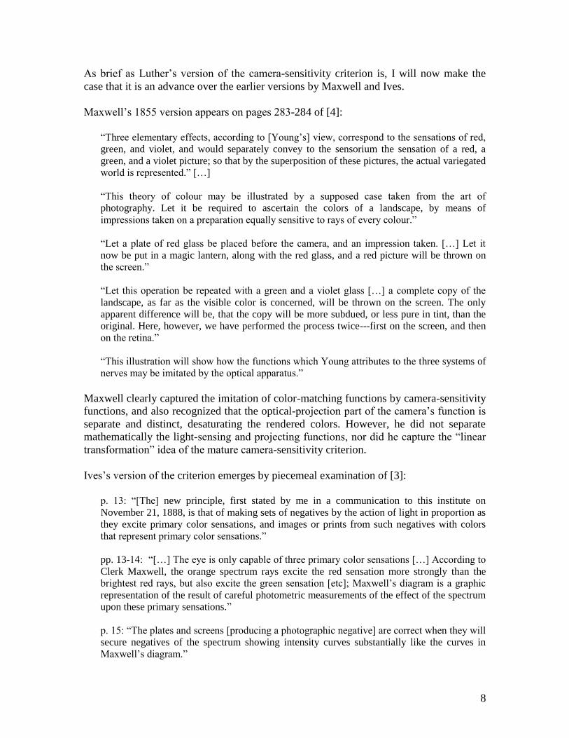
As brief as Luther‟s version of the camera-sensitivity criterion is, I will now make the

case that it is an advance over the earlier versions by Maxwell and Ives.

Maxwell‟s 1855 version appears on pages 283-284 of [4]:

“Three elementary effects, according to [Young‟s] view, correspond to the sensations of red,

green, and violet, and would separately convey to the sensorium the sensation of a red, a

green, and a violet picture; so that by the superposition of these pictures, the actual variegated

world is represented.” […]

“This theory of colour may be illustrated by a supposed case taken from the art of

photography. Let it be required to ascertain the colors of a landscape, by means of

impressions taken on a preparation equally sensitive to rays of every colour.”

“Let a plate of red glass be placed before the camera, and an impression taken. […] Let it

now be put in a magic lantern, along with the red glass, and a red picture will be thrown on

the screen.”

“Let this operation be repeated with a green and a violet glass […] a complete copy of the

landscape, as far as the visible color is concerned, will be thrown on the screen. The only

apparent difference will be, that the copy will be more subdued, or less pure in tint, than the

original. Here, however, we have performed the process twice---first on the screen, and then

on the retina.”

“This illustration will show how the functions which Young attributes to the three systems of

nerves may be imitated by the optical apparatus.”

Maxwell clearly captured the imitation of color-matching functions by camera-sensitivity

functions, and also recognized that the optical-projection part of the camera‟s function is

separate and distinct, desaturating the rendered colors. However, he did not separate

mathematically the light-sensing and projecting functions, nor did he capture the “linear

transformation” idea of the mature camera-sensitivity criterion.

Ives‟s version of the criterion emerges by piecemeal examination of [3]:

p. 13: “[The] new principle, first stated by me in a communication to this institute on

November 21, 1888, is that of making sets of negatives by the action of light in proportion as

they excite primary color sensations, and images or prints from such negatives with colors

that represent primary color sensations.”

pp. 13-14: “[…] The eye is only capable of three primary color sensations […] According to

Clerk Maxwell, the orange spectrum rays excite the red sensation more strongly than the

brightest red rays, but also excite the green sensation [etc]; Maxwell‟s diagram is a graphic

representation of the result of careful photometric measurements of the effect of the spectrum

upon these primary sensations.”

p. 15: “The plates and screens [producing a photographic negative] are correct when they will

secure negatives of the spectrum showing intensity curves substantially like the curves in

Maxwell‟s diagram.”

9

Ives clearly separated the sensing function of the camera from the rendering function, and

attributed the imitation of visual sensitivity firmly to the former. The linear

transformation idea was still not on the horizon.

Given these earlier works, it is not far-fetched to consider Luther‟s contribution a further

step toward the mature criterion: a mathematical equation, and a precise though brief

discussion of the equation. The linear-transformation freedom, however, is still not

acknowledged.

Lest we consider that Luther missed an obvious point, it is instructive to see how later

authors incorporated the linear-transformation freedom. That property was clearly

understood by Neugebauer in 1956 [7]. But consider MacAdam‟s 1967 work [4]:

p. 28: “Maxwell was quite specific about the required character of the controls. He said that

three photographs should be made with spectral sensitivities proportional to the three spectral

sensitivities had shown can be attributed to the eye to account for all of the infinite varieties

of spectral distributions that can look alike (that is, „have the same color‟).”

In the next paragraph: ”Thirty years later, Frederic Ives had much more suitable materials,

and also the single-minded persistence required to carry out Maxwell‟s idea and to

demonstrate its validity to a skeptical and even hostile audience. But his success has little

influence on the development of modern color photography. Through his son Herbert,

however, it had a significant influence on the modern technology of color measurement that

very effectively supplements spectroscopy (spectrophotometry) in all industries that supply

colored products.”

Although MacAdam‟s words are accurate, the statement “proportional to the three

spectral sensitivities” leaves unexpressed the freedom of linear transformation. It is a

subtlety that gained significant attention only when computers became commonly

available to exercise the linear transformation freedom.

I found it quite educational to examine in this way the contribution of Maxwell, Ives, and

Luther of the camera criterion that bears various combinations of their names. The

earliest inventors of an idea did not necessarily grasp or express its complete essence.

There may even be a fragment today that we are not using to complete advantage.

4. Conclusions

This introduction has been a whirlwind tour of Luther‟s article followed by two highly

focused micro-views. It cannot be said that I have “stolen the thunder” of the article or

given away the ending. Luther‟s article is the work of a scholar of great accomplishment

but terse expression, who has summarized color science as of the third decade of the 20th

Century in one diverse essay. Enjoy!

Michael H. Brill

Datacolor

10

[1] R. Luther, Aus dem Gebiet der Farbreizmetrik, Z. Technische Physik., 8, 540-558

(1927). [English translation by Rolf G. Kuehni, 2009].

[2] J. C. Maxwell, Experiments on Colour as perceived by the eye with remarks on colour

blindness. Edinburgh Royal Society Transactions. XXI, 1857, pp. 275-298. [1855].

Scientific Papers Vol. 1 pp. 126-154. See pp. 283-284 for the statement about camera

sensitivities.

[3] Frederic E. Ives, Photography in the colors of nature, J. Franklin Inst. 131, 1-21

(1891).

[4] David L MacAdam, “Color Science and Color Photography”, Physics Today, January

1967, pp. 27-39.

[5] Francisco Martínez-Verdú et al., “Concerning the calculation of the color gamut in a

digital camera,” Color Research and Application 31, 399-410 (2006).

[6] M. Richter, I. Schmidt, A. Dresler, Grundriss der Farbenlehre der Gegenwart,

Dresden: Theodor Steinkopff, 1940, p141.

[7] H. E. J. Neugebauer, "Quality factor for filters whose spectral transmittances are

different from color mixture curves, and its application to color photography," J. Opt.

Soc. Amer., 46 (1956), 821-824.

11

On color stimulus metrics by R. Luther, Dresden

Zeitschrift für Technische Physik, 1927, Vol. 8, Nr. 12, 540-558

Contents: In the first part, by expanding classical color theory and use of the unit „color

moment‟, new parameter triads are developed and used to produce three-dimensional

color solids, particularly useful to represent the chromatic properties of object colors. In

the second part, related to color measurement technology, heterochromatic photometry,

and three-color photography are discussed.

1. Given time limitations, I am unable to provide a logically developed, comprehensive

survey but – as already the title of my presentation indicates – only more or less loosely

arranged excerpts from the field of color science. Any such selection is indicative of

personal preferences and for this reason I would like to briefly describe the foundations

of the present one.

I would like to particularly emphasize that my expositions and reflections have

their source in practical, technical questions of my field of specialty, which lead into the

same questions: theory of color photography; of anaglyphs, of orthochromatics, and its

opposite pole: darkroom illumination, methods of color measurement, and of

heterochromatic photometry. In agreement with the title of my presentation I will concern

myself almost exclusively with what v. Kries names color stimuli – in contrast to the

color perceptions that they cause. I will in general remain in the purview of Schrödinger‟s

basic colorimetry,1 but also make use of the term heterochromatic brightness. I will not

concern myself with the so-called theories of color vision – Helmholtz, Hering, v. Kries. I

will attempt to present preferably unknown or, to my best knowledge, little know

subjects. I will reach back into classical representations of color theory only to the extent

that this is absolutely necessary, all the more because recently several summaries2 of that

theory have been published.

If, according to Ostwald, we term color stimuli that under identical conditions

result in identical percepts but objectively have different spectral compositions as

“metamers,” we can define classical color theory in an abbreviated way as the theory of

the generation of metameric – chromatic as well as achromatic – color stimuli.

2. It is known that under certain limiting conditions: cone vision, average color-normal

eye, limitation to “reduced” colors in the sense of D. Katz3 – the totality of here

applicable relationships is of threefold diversity. A given color stimulus can therefore be

completely defined by its properties in terms of three suitably defined independent

parameters.

Once a triad of parameters has been selected it is, of course, possible to derive

from them an arbitrarily large number of new triads that express the same complex of

facts with identical completeness and that are equally suitable for the definition of a color

stimulus.

The first part of my presentation concerns itself, among other things, with some as

yet not employed parameter triads.4 The selection, out of a limitless number of

possibilities, has been made less for the purpose of achieving maximal generality but

rather is based on a point of view of practicality. Only systems that are sufficiently

12

informative, systems that make it possible to comprehend as many relationships as

possible in the simplest possible manner, those that simplify practical work, and finally –

as much as possible – demonstrate new connections are to be considered. I will not

mention closely related derivations and generalizations.

3. My basis is the well-known Young-Helmholtz-Maxwell, so-called trichromatic,

system. In that system every color stimulus, arbitrarily composed from spectral stimuli, is

unambiguously defined by the “amounts” of three independent, but otherwise arbitrarily

selectable, elementary or – according to v. Kries – “primary” stimuli [Eichreize].

As all mixed stimuli, in the final analysis, are composed of spectral stimuli the

first step is a “spectrum standardization” (v. Kries). Figure 1 top shows such a

“standardization” of the daylight spectrum,5 as first determined by Maxwell. The

abscissas represent the wavelengths of the standard spectrum, the ordinates the amounts

of the R, G, and B of the three selected primary stimuli Red, Green, and Blue, as well as

their sum S = R + G + B, for identically narrow spectral ranges of always 10 nanometers.

The amounts of the three primary stimuli, together resulting in white, are as usual

of identical magnitude, each equaling 1000 stimulus units. As a result, white composed

from the total spectrum, independent of its absolute brightness, has the stimulus sum of

S = dS )(

380

700

= 3000 stimulus units

The identity of the amounts of the three primary stimuli in white is expressed in the areal

identity of the areas between the three primary functions and the abscissa axis in the top

part of Fig. 1:

R = dR )(

380

700

= G = dG )(

380

700

= B = dB )(

380

700

= 1000.

In case of an arbitrary mixed stimulus, i. e. a mixture of spectral stimuli such as that of

the emerald [Smaragd] measured by Exner, as illuminated by daylight reflected into the

eye, the amounts of the three primary stimuli can, as is well known, be easily calculated

from the reflectance spectrum (Fig. 1 bottom). To achieve this, for a sufficiently large

number of wavelengths the ordinate values of the primary stimuli have to be multiplied

with the fractions of the illuminating light Rm (λ) reflected at the same wavelengths and

the size of the resulting area determined, e.g. for the red stimulus.

R Sm = dRmR Sm )()(

380

700

.

4. When many sets of standard stimuli have to be calculated it is possible to simplify the

work, e.g. when determining RSm, by arranging the spectrum on the abscissa axis in such

a way that equal increments of the abscissa correspond to equal increments of the red

stimulus in the daylight spectrum. To achieve this, one integrates the R function of Fig. 1

13

relative to λ and in this way obtains, as shown in Fig. 2, the required division of the

spectrum. The same procedure is applied to the G and B functions and, for control

purposes, possibly also to the S function.

If in the once and for all determined coordinate systems the unit of the ordinate is

selected to be the same as that of the reflection spectrum, the ordinates of such a

spectrum can be transformed without recalculation. The resulting areas7 correspond now

to the amounts of the three primary stimuli. Figure 3 shows this procedure for the

reflectance spectrum of the emerald in schematic form.

For the present case the result is that the mixture stimulus caused by the emerald

consists in total of 713 stimulus units, divided into 198 R units, 317 G units, and 198 B

units.

Fig. 1. (left) Calibration of the daylight spectrum and determination of the three primary stimulus

amounts in the spectrum of a mixed stimulus (reflectance of an emerald).

[Reizeinheiten je 10 μμ: stimulus units per 10 nm; Smaragd_Remission: reflectance of an

emerald]

Fig. 2. (right) Separation of the spectrum according to equal increments of the red stimulus.

5. These numbers provide a complete but not easily comprehended picture of the

characteristic appearance of the color of the emerald. Comprehension is improved by

plotting the components of the three primary stimuli of spectral as well as mixed stimuli

such as that of the emerald:

S

Rr ,

S

Gg and

S

Bb

as triangular coordinates into an equilateral triangle (Fig. 4 top). For the emerald the

values are rSm = 0.28; gSm = 0.44; bSm = 0.28.

Plotting the spectral stimuli into the chromatic diagram has, in terms of Newton‟s

center of gravity construct, the following easy-to-grasp significance: Assume that red,

green, and blue weights proportional to the amounts of the corresponding ordinate values

14

of the three spectral primary stimuli of Fig. 1 hang at every 10 nm interval along the

spectral curve in the chromatic diagram. The result is that the system supported at the

white or achromatic point U [Unbundt] – the center of gravity – is in balance. The weight

pulling on the balance point is equal to the sum of all individual weights (i. e. the

stimulus sum of white). The weights at each spectral wavelength can be removed and re-

attached at the corresponding corner points without upsetting the balance. The white or

achromatic point corresponds to a state of balance of the chromatic spectral stimuli,

where they compensate each other, with none of them predominating.

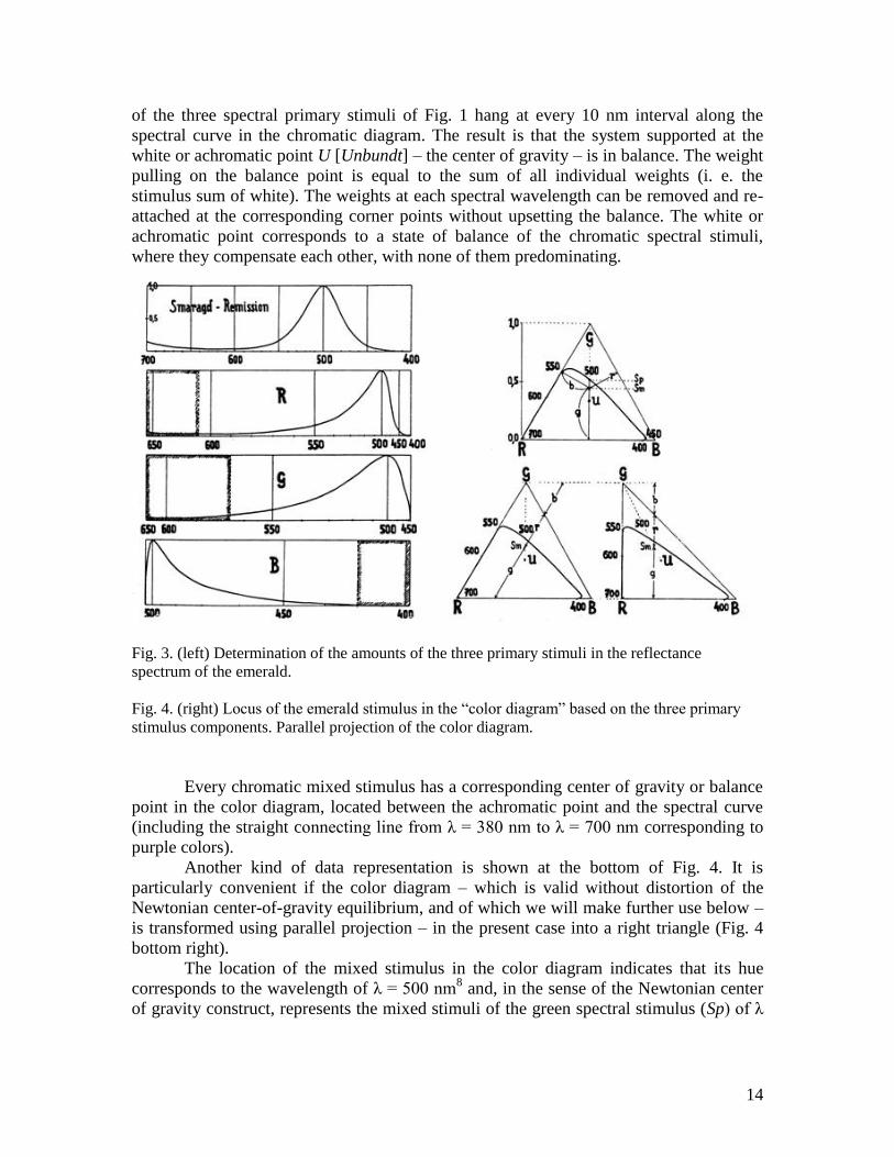
Fig. 3. (left) Determination of the amounts of the three primary stimuli in the reflectance

spectrum of the emerald.

Fig. 4. (right) Locus of the emerald stimulus in the “color diagram” based on the three primary

stimulus components. Parallel projection of the color diagram.

Every chromatic mixed stimulus has a corresponding center of gravity or balance

point in the color diagram, located between the achromatic point and the spectral curve

(including the straight connecting line from λ = 380 nm to λ = 700 nm corresponding to

purple colors).

Another kind of data representation is shown at the bottom of Fig. 4. It is

particularly convenient if the color diagram – which is valid without distortion of the

Newtonian center-of-gravity equilibrium, and of which we will make further use below –

is transformed using parallel projection – in the present case into a right triangle (Fig. 4

bottom right).

The location of the mixed stimulus in the color diagram indicates that its hue

corresponds to the wavelength of λ = 500 nm8 and, in the sense of the Newtonian center

of gravity construct, represents the mixed stimuli of the green spectral stimulus (Sp) of λ

15

= 500 nm and of the achromatic center (U). The relative amounts of spectral and

achromatic stimuli in the total stimulus is obtained from the lever ratios

SpU

SmU

and

SpU

SpSm

(see Fig. 4 top).

For the emerald the result is that of the sum total of 713 stimulus units of the complete

stimulus 40% are due to the achromatic stimulus and the remaining 60% due to the

spectral stimulus λ = 500 nm. The latter component 0.60 is called “saturation,” or “color

saturation” (in stimulus units).

By reporting hue, saturation, and ”intensity”, i.e., the total weight in the

Newtonian sense, the totality of the stimulus in stimulus units, we obtain the Grassmann-

Helmholtz parameter triad 9, thereby resulting in an unambiguous and easy to

comprehend definition of the color stimulus.10

6. Unsatisfactory and distracting is the calculation of “intensity” and of saturation in

stimulus units, leftovers from a particular trichromatic system not otherwise present in

the Grassmann-Helmholtz system. Already early (Grassmann), the need arose to replace

the arbitrarily selected stimulus units as a measure of intensity with an experimental,

independently determinable unit of measurement: brightness (more correctly: surface

brightness). Here I do not want to concern myself with v. Kries‟ critique of the term

heterochromatic brightness, as well as Schrödinger‟s related comments (note 1), but

rather limit myself to the experimental data.

In regard to the dependence of specific brightness Hλ of the spectral stimuli on

wavelength, all methodologies of heterochromatic brightness determination used by Ives‟

in his systematic experiments,11

with one exception,12

essentially agreed in the final

result, if with very different variability. An additional result was that on a practical level,

i.e., within the unavoidable errors of measurement and individual variation, the

brightness values measured in this manner are purely additive.13

If one assumes the existence of a brightness H, measurable independent of hue

and saturation, and with the additive property H = dH in stimulus summation, it

follows that brightness H of an arbitrarily composed stimulus can be calculated from the

amounts of the reference stimuli contained in it, using a linear formula:

H = ρR + γ G + β B.

It should be noted here that in case of the usual choice of the three reference

stimuli (red, green, and blue) the factor β – the specific brightness of the blue reference

stimulus – is always very small compared to ρ and γ.

7. What are the resulting changes for the spectral reference functions and the color

diagram?

In case of the spectral reference functions the ordinates obviously have to be

multiplied with the corresponding coefficients ρ, γ, and β. As a result, the stimulus sum

function S takes on the form of the brightness sum function, i.e., the so-called spectral

brightness function H (Fig. 5 bottom).

16

The change in the color diagram can be represented using the following idea that

will later come in handy in another form.

Fig. 5. Schematic representation of the change in the color diagram (top) and the primary

stimulus curves (bottom) when changing from calculation in stimulus units to one in brightness

units. The polar moment curve M remains unchanged. The stimulus sum curve S changes to the

brightness curve H. The dashed parts of the two upper figures are related according to the ratio of

central perspectives.

[Rz.-Einh.: stimulus units; Hell.-Einh.: brightness units]

The (“leucocentric”[white-centered]) lines drawn in intervals of 10 nm from the

achromatic point to the spectral curve of the color diagram can, in the sense of a

Newtonian center of gravity construct, be viewed as a system of solidly connected levers,

supported at the achromatic point, at the ends of which hang as weights the stimulus sums

of the individual 10-nm spectral intervals.

If the Newtonian center of gravity is not to be disturbed when replacing stimulus

units with brightness units, neither for the spectral stimuli nor for the reference stimuli,

this can, seemingly in the simplest way, be achieved as follows: all levers (= leucocentric

lines) without change in direction and corresponding to the new weights attached to them

are also changed in their length in a related manner so that the product of length of lever

and weight, i.e. the leucocentric lever moment, remains unchanged.

Figure 5 schematically shows this change from counting the weights in stimulus

units to counting them in brightness units. The change in the three spectral primary

stimulus curves and the change from the stimulus sum curve S to the spectral brightness

curve H is indicated on the bottom – the corresponding change in the color diagram is

shown on top.14

It is obvious that the levers to which the blue stimulus is attached, while

not changing in direction, are increasing in length, corresponding with the very small

“specific weight” of the blue stimulus.

The spectral lever moments remain unchanged in this transition from one color

diagram to the other and are drawn leucocentrically polar with full line M (of retort

shape) in both color diagrams.15

However, the stimulus sum curve S, shown also in polar

form with a finely dotted line in the upper left diagram, changes to the correspondingly

represented spectral brightness curve H16

in the right color diagram.17

17

The transformation coefficients ρ, γ, and β depend on the choice of the primary

stimuli. Depending on the conditions, the always very small coefficient β can have a

value of zero or even be negative.18

My three primary stimuli have been chosen in a

manner that β = 0,19

i.e. the infinitely small weight of the blue primary stimulus is

attached to an infinitely long lever: the lever moment does not change its finite value.

Relative to the new brightness values the characteristic numbers for the emerald

in the Grassmann-Helmholtz “monochromatic” system are: brightness = 0.26 of the total

spectrum of 515 brightness units, saturation = 0.63.

8. Introduction of the moments allows construction of a new triad of parameters that

offers, in addition to ease of comprehension, many advantages.

It is possible to relate the Newtonian center of gravity of a mixed stimulus to two

axes rather than to three points, the loci of the three primary stimuli in the color diagram.

The two axes are not parallel in the plane of the color diagram and the torques applied by

the individual weights on them can be made the basis of the calculation.20

In agreement with the psychological arrangement of the hues – the so-called four-

color system – I place the two axes through the achromatic point in the direction Green-

Purple and Blue-Yellow and, to aid comprehension and in agreement with Fig. 6, change

the obliquely angled axes into right-angled ones using parallel projection (whereby the

weights remain unchanged). If we now consider each leucocentric moment to be reduced

to its right-angled components, that is into the torques for the two axes Green-Purple and

Blue-Yellow we obtain the following relationships.

Fig. 6. Parallel projective transformation of the equilateral color diagram with tilted moment axes

into a color diagram with rectangular moment axes. Additional transformation into a color

diagram based on brightness units (top right, reduced scale). The specific brightness of the blue

stimulus is equal to 0.

18

The torques of all weights that, for example, are applicable on the right side of the

Green-Purple axis correspond in their totality to a – in two words – bluish torque, or the

“blueness” – to use one of Hering‟s expressions. Opposed to this blueness are the

“yellowish” torques of the weights active on the left of the Green-Purple axis, the total

torque of which – again after Hering – can be termed the “yellowness” of a mixed

stimulus. If yellowness exceeds blueness the total moment corresponds to a yellowish

hue, and vice versa. If both are identical, that is the total moment is zero, the result

corresponds to a hue that is neither bluish nor yellowish and can only lie on the Green-

Purple line. What is decisive is the difference: blueness minus yellowness.

The identical idea can be applied to the to Green-Purple moments acting on the

Blue-Yellow axis and one can speak, in agreement with Hering, of greenness-redness,

that is, greenness minus redness. (Hering‟s Red, less yellowish and more purplish than

the primary red that I also call Red, will be distinguished from the latter by the addition

of [H].

The two moments Greenness-R[H]edness and Blueness-Yellowness, together

with the “weight” of a stimulus, either expressed in stimulus or in brightness units, form a

new parameter triad21

with which a given color stimulus can be defined uniquely and in a

manner that is quite easy to comprehend.

Of course, the two torques add up like vectors and, with the sign and the amount

of their ratios, show their direction in the color diagram, thereby showing the hue of the

resulting leucocentric color moment in a comprehensible manner. In an analogous

manner one might call the result “colorfulness.” By dividing the leucocentric color

moment by the “weight” of the stimulus the length of the leucocentric lever is obtained,

from which its saturation and the shares and amounts of the three primary stimuli are

immediately available. This method represents the reciprocal conversion key of the tetra-

tri-, and monochromatic systems.

9. In case of a composite mixed stimulus, for example an absorption or reflectance

spectrum – such as our emerald spectrum – we can as before (paragraph 3) extract the

two reference moments as well as the total stimulus or the brightness, respectively. To

achieve this, first the amounts of the two reference moments are plotted at 10 nm

intervals as ordinates in the standard spectrum. The resulting curves (Fig. 7) can be

calculated from the corresponding amounts of the reference stimuli according to the

linear formula22

M = mR + nG + pB. (The area between the abscissa axis and the

R(H)ed moment curve, that is, the sum of all spectral R(H)ed moments is of the same size

but opposite sign compared to the corresponding area of the Green moment curve and the

same applies for the areas under the Blue and Yellow moment curves because the two

reference moments of the total achromatic spectrum equal 0.)

When multiplying, for a sufficiently large number of wavelengths, the ordinates

of this curve with the reflectance values of the emerald and calculating – considering the

sign – the total area, the two total moments of the emerald stimulus are obtained. The

same applies to the stimulus sum curve S and the brightness curve H, respectively.23

On making these calculations (see dashed lines in Fig. 7) according to the

parameter values I selected, the following characteristics of the color of the emerald are

obtained: Blueness-Yellowness = 0; Greenness-R(H)edness = 79 moment units; weight =

19

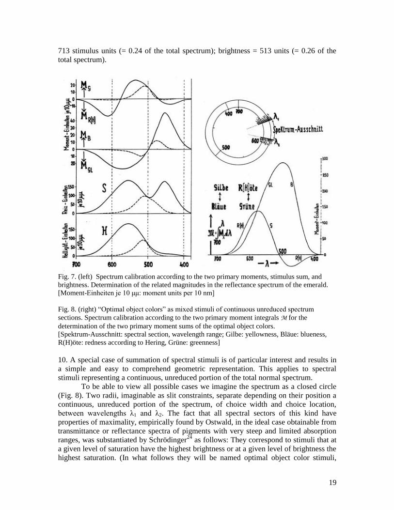
713 stimulus units (= 0.24 of the total spectrum); brightness = 513 units (= 0.26 of the

total spectrum).

Fig. 7. (left) Spectrum calibration according to the two primary moments, stimulus sum, and

brightness. Determination of the related magnitudes in the reflectance spectrum of the emerald.

[Moment-Einheiten je 10 μμ: moment units per 10 nm]

Fig. 8. (right) “Optimal object colors” as mixed stimuli of continuous unreduced spectrum

sections. Spectrum calibration according to the two primary moment integrals M for the

determination of the two primary moment sums of the optimal object colors.

[Spektrum-Ausschnitt: spectral section, wavelength range; Gilbe: yellowness, Bläue: blueness,

R(H)öte: redness according to Hering, Grüne: greenness]

10. A special case of summation of spectral stimuli is of particular interest and results in

a simple and easy to comprehend geometric representation. This applies to spectral

stimuli representing a continuous, unreduced portion of the total normal spectrum.

To be able to view all possible cases we imagine the spectrum as a closed circle

(Fig. 8). Two radii, imaginable as slit constraints, separate depending on their position a

continuous, unreduced portion of the spectrum, of choice width and choice location,

between wavelengths λ1 and λ2. The fact that all spectral sectors of this kind have

properties of maximality, empirically found by Ostwald, in the ideal case obtainable from

transmittance or reflectance spectra of pigments with very steep and limited absorption

ranges, was substantiated by Schrödinger24

as follows: They correspond to stimuli that at

a given level of saturation have the highest brightness or at a given level of brightness the

highest saturation. (In what follows they will be named optimal object color stimuli,

20

abbreviated optimal colors.) All other object color stimuli can be obtained by darkening

the optimal colors.

The two wavelengths λ1 and λ2 together with the absolute, related to the total

spectrum, or the relative, related to optimal color, “intensity” – for example in brightness

units – offer again a triad of parameters sufficient for the complete description of a color

stimulus25

and for the reproduction of that stimulus with a suitable apparatus – for

example the Maxwell-Ostwald color mixer. Here I would like to provide the data for the

emerald: λ1 = 561 nm, λ2 = 458 nm, brightness = 0.50 of the optimal color = 0.26 of the

total spectrum.

The geometric representation of the triad: brightness, λ1 and λ2 – perhaps to be

called the “dichromatic system – is not easy to comprehend, however the following

considerations point the way to a representation that is easy to comprehend.

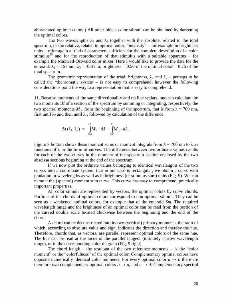
11. Because moments of the same directionality add up like scalars, one can calculate the

two moments M of a section of the spectrum by summing or integrating, respectively, the

two spectral moments M λ from the beginning of the spectrum, that is from λ = 700 nm,

first until λ2 and then until λ1, followed by calculation of the difference

M (λ1..λ2) =

dMdM 1

700

2

700

.

Figure 8 bottom shows these moment sums or moment integrals from λ = 700 nm to λ as

functions of λ in the form of curves. The difference between two ordinate values results

for each of the two curves in the moment of the spectrum section enclosed by the two

abscissa sections beginning at the end of the spectrum.

If we now plot the ordinate values belonging to identical wavelengths of the two

curves into a coordinate system, that in our case is rectangular, we obtain a curve with

gradation in wavelengths as well as in brightness (or stimulus sum) units (Fig. 9). We can

name it the (spectral) moment sum curve. This curve has easy to comprehend, practically

important properties.

All color stimuli are represented by vectors, the optimal colors by curve chords.

Portions of the chords of optimal colors correspond to non-optimal stimuli. They can be

seen as a weakened optimal colors, for example that of the emerald Sm. The required

wavelength range and the brightness of an optimal color can be read from the portion of

the curved double scale located clockwise between the beginning and the end of the

chord.

A chord can be deconstructed into its two (vertical) primary moments, the ratio of

which, according to absolute value and sign, indicates the direction and thereby the hue.

Therefore, chords that, as vectors, are parallel represent optimal colors of the same hue.

The hue can be read at the locus of the parallel tangent (infinitely narrow wavelength

range), or in the corresponding color diagram (Fig. 9 right).

The chord length – the resultant of the two reference moments – is the “color

moment” or the “colorfulness” of the optimal color. Complementary optimal colors have

opposite numerically identical color moments. For every optimal color a → b there are

therefore two complementary optimal colors b → a, and c → d. Complementary spectral

21

colors, that is, optimal colors of infinitely narrow wavelength range, therefore have

parallel tangents of opposite direction.

12. Parallel shifting of a chord can, according to the above, be useful for the convenient

determination of the spectral width in case of “isochromatic” widening of the width, that

is, while maintaining the same hue. In case of a parallel shift of this kind the chord

length, that is, the colorfulness or the color moment, changes from the value zero

(infinitely narrow spectral width) via a maximum V all the way again to zero (total

spectrum). The maximal chord length, that is the maximal “colorfulness,” corresponds to

Ostwald‟s full colors, because when maximal values are attained the curve is sectioned

either at two complementary points with parallel tangents or in the corner (see figure).

The chord length, the color moment, or the colorfulness can be made

comprehensible by using the following consideration. If we take the lightness of an

optimal color to be, in the Newtonian sense, its “weight,” the following relations apply:

Moment of optimal color/weight of optimal color = length of lever of optimal color in the

color diagram.

Length of lever of optimal color/length of lever of spectral color = saturation, i.e., share

of spectral color in the optimal color.

Weight of optimal color ∙ saturation = weight of spectral color in the optimal color.

Therefore:

Moment of optimal color = length of lever of the spectral color ∙ weight of the

spectral color in the optimal color.

The chord length (= moment of the optimal color) is therefore proportional to the

amount of spectral stimulus in the optimal color stimulus. The proportionality factor, the

lever of the spectral stimulus, naturally depends on hue and the selected amounts and

measurement units. But it is constant for a give hue, that is, for a group of parallel chords

of equal direction.

Ostwald‟s full colors are, in the sense of classical color metrics, distinguished by

containing the maximum amount of spectral stimulus that the most perfect pigments can

have: as a result, also in the sense of classical color science they represent “exceptional

cases.”

13. The moment sum curve of Fig. 9 (see also Figs. 10 and 13) contains a few additional

chords that show an example of the application of the spectral moment sum curve when

solving a practical problem. A colorant with the two complementary spectral ranges ab

and cd is a so-called invalid gray. The same is true for another colorant with the spectral

ranges bc and da, because it also results in an invalid gray, one that is “complementary”

to the first one. Anaglyphs produced using such “complementary‟ false-gray pigments

would offer an interesting kind of image: when viewed with a gray set of glasses, out of a

confusion of gray lines an object would begin to appear in three dimensions. A. Callier26

has produced and demonstrated such complementary false-gray filters. To a high degree

22

they have the annoying property of making the yellow spot entoptically visible. In

addition, their color depends very much on the spectral composition of the light as well as

on the adaptation and the individual properties of the viewing eye. All these properties

can be used for measuring purposes.

Much more might be said in regard to this “moment sum curve.” However, while

making use of it, I will limit myself to the construction of three solids particularly

suitable to represent the properties of object colors.

Fig. 9. Moment sum curves with dual scales in wavelength and brightness units and their

relationship to the color diagram. Vectorially parallel chords correspond to optimal object colors

of the same hue. The portion of the double scale located clockwise between beginning and end of

a chord indicates the open region of the wavelength range. The cord length is equal to the “color

moment” and proportional to the content of spectral stimulus. Ostwald‟s full colors V are imbued

with maximal color moment and spectral stimulus and section the curve either at complementary

wavelengths, i. e., at points with parallel but opposite directed tangents, or in the corner.

Representation of two “complementary” invalid gray filters for stereoscopy. Representation of the

emerald stimulus as weakened optimal object color.

14. Figure 10 shows sections through a solid that correspond to four different hues. The

corresponding three rectangular coordinates of the solid represent hue, saturation, and

brightness. Because in each of the shown sections hue is constant they are variable in

regard to saturation and brightness. Saturation is represented by the ordinate, brightness

by the abscissa, counted from the left incline of the (solid) curve toward the right. On the

left the inclining curves represent brightness zero. Optimal colors are located on the right

declining curve. Their brightness is represented by the horizontal distance from the left

“black” incline, their saturation by the ordinate. In addition, the two limiting wavelengths

of the optimal colors can be read from the intersection points of the horizontal lines (of

equal saturation), projected with vertical lines onto the abscissa axis, and the

23

corresponding wavelengths (see curve for Green-Blue 490). For this purpose, the abscissa

axis has an equiluminant wavelength scale (see Note 23), the start of which obviously

depends on the hue represented by the section.

Fig. 10. Four sections through a three-dimensional solid valid for object colors, with the

coordinates hue, saturation, brightness. The abscissa is scaled by an equiluminous spectrum; the

left inclines correspond to brightness equals 0, the dashed curve section on the right contain the

optimal object colors. Representation of the emerald color Sm as a darkened optimal object color

OSm. Graphic determination of the amount of spectral stimulus in the emerald stimulus. The

maximal spectral stimulus is contained in optimal object colors. (Section Green-Blue 490).

Exceptional situation in case of yellow optimal object colors.

[Spektr.: spectral stimulus, Unb.: achromatic stimulus, Sättigung: saturation, Schwarz: black,

Helligkeit: brightness, Optimal Farbe: optimal object color stimulus]

The brightness of the spectral portion of an optimal color equals the product of its

brightness and saturation. This brightness of the spectral component is represented by the

areas of the rectangles shown in the curve Green-Blue 490. For narrow wavelength

ranges the area is small but grows with decreasing saturation and increasing brightness

due to the widening of the section. A maximum is reached in case of Ostwald‟s full

colors. Further widening of the wavelength range results in reduction of the area all the

way to the situation where the section encompasses the complete spectrum (saturation =

0) and the area is equal to zero.

Non-optimal color stimuli (for example that of the emerald Sm), they can be

considered to be darkened optimal color stimuli, are located on the horizontal line

corresponding to their optimal color (OSm) in the direction of the left (black) incline (see

curve Green 500). Horizontal lines, therefore, are lines of constant saturation and

constant hue, that is, of constant color character, respectively chroma, respectively

stimulus type; they are identical with Ostwald‟s “shadow series”. In case of the emerald

stimulus, geometrically as a matter of course, its total brightness has been divided into the

brightness of the spectral (Spektr.) and the achromatic (Unb.) portions.

24

From the different shapes of the four curves one can deduce the changes in

relations in different hues in regard to changes in brightness and saturation. It is evident

that yellow object colors represent a special case. Here the full color, with a brightness of

over 85% of the total spectrum is nearly (≈98%) fully saturated, contrary to R(H)ed,

where the full color is very dark and has little saturation. It is further evident that if one of

the limiting wavelengths passes through the end of the spectrum the result is a bend in the

ascending, opposite end of the curve (curve GB 490).

Fig. 11. Parallel-perspective representation of the solid discussed in Fig. 10.

[Farbton: hue]

Figure 11 is a perspectival representation of a series of sections located above two

connecting equiluminous spectral scales.

15. Another “object color stimulus solid” with the rectangular coordinates Blueness-

Yellowness, Greenness-R(H)edness, and stimulus sum in one case, brightness in the

other, is shown in Figs. 12, 13, and 14. On top of Fig. 12 and in Fig. 14 the vertical scale

is in stimulus units; in Fig. 12 bottom and Fig. 13 the vertical scale is in brightness units.

The shape of the solid is reminiscent of a parallelepiped with rounded corners and usually

positively rounded planes. Its center of symmetry is binomial.

The null point of the coordinate system resides in the achromatic “black point,”

having zero stimulus or brightness. The achromatic axis, having a color moment of zero

rises from black via gray to white. A color stimulus corresponds to every point not on the

axis but within the solid. Its stimulus sum, respectively brightness, can be read from its

vertical coordinate, its hue from the ratio, and its color moment from the resultant of the

two horizontal coordinates. Correspondingly, the points of highest colorfulness at a given

level of brightness, respectively stimulus sum, are located on the surface of the solid. The

points representing all other object color stimuli are located in its interior.

In the additive mixture of two stimuli their Blue-Yellow moments, their Green

R(H)ed moments, and their brightnesses, respectively stimulus sums, are added up. In

other words: The vectors drawn from the point of origin to the two points are added up in

a vector parallelogram. Therefore, every stimulus can, in the sense of the Grassmann-

25

Maxwell vectorial representation, be seen as a vector (see also Pilgrim op. cit.). In case of

proportional mixture of two stimuli (for example in case of disk mixture) the resulting

mixed stimuli are located on the straight line connecting the two stimulus points, their

distances from these are inversely proportional to their shares in the total stimulus.

Fig. 12. Perspective representation of the “optimal object color solid,” similar to a parallelepiped,

with the horizontal coordinates Blueness-Yellowness, Greenness-R(H)edness and the vertical

coordinate brightness (top row), stimulus sum (upper row). The meridians of the lower row, with

angular difference of approximately 45º, correspond to the sections in the following Fig. 13.

Ostwald‟s full colors are projected onto the horizontal coordinate plane by the mantel of a vertical

cylinder touching the surface of the solid.

26

Fig. 13. Four axial sections, corresponding to meridians separated by 45º, through the optimal

object color solid of Fig. 12 bottom in brightness units with a common black-white axis and

common dual symmetry center Z. The sections correspond to the hues Green500 - R(H)ed500 (top

left); Orange605 - Green-Blue490 (top right); Yellow576 – Blue470 (bottom left) and Yellow-

Green547 – Purple-Violet-547 (bottom right). Determination (top left) of saturation

Smp

kp

SpU

SmU

and the amount of spectral stimulus p – k in the total brightness p – Sm of

the emerald stimulus. Determination of the emerald stimulus Sm by darkening of its optimal color

OSm. Representation (top right) of the optimal object colors shown in Fig. 9 with full lines.

Representation (bottom right) of Ostwald‟s triad (hue, and two of the components white, black,

full color) and of the colors missing in Ostwald‟s system (hatched areas). Representation (bottom

right) of the totality of the stimuli complementary to stimulus F. Exceptional status of yellow

object colors.

[Weiss: white, Vollfarbe: full color, Kompl. zu F: complement to F]

16. Every axial section contains the totality of all object color stimuli of two

complementary hues. Figure 13 shows four such sections through the solid (in brightness

units). In all four sections the mid-point of the black-white axis Z is the binomial center

of symmetry because two optimal colors that together fill the complete spectrum have

identical but opposite color moments, thereby being symmetrical in regard to the center

point.

The null point of the coordinate count, – the “black point,” – corresponds to

infinitely narrow wavelength ranges. Widening of the section results in increases in color

moment and brightness in the same sense (see Orange and Green-Blue sections) until the

color moment reaches a maximum at the point of Ostwald‟s full colors (V). Further

widening results in a complete spectrum being permitted to pass – at the white point –

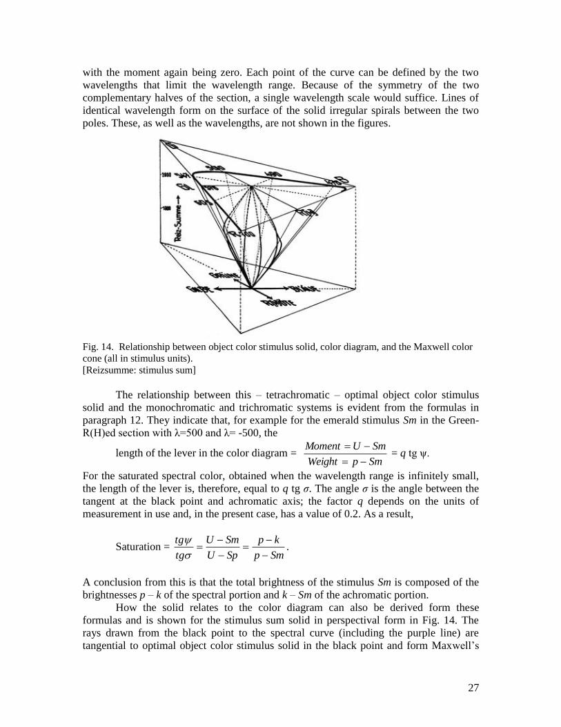
27

with the moment again being zero. Each point of the curve can be defined by the two

wavelengths that limit the wavelength range. Because of the symmetry of the two

complementary halves of the section, a single wavelength scale would suffice. Lines of

identical wavelength form on the surface of the solid irregular spirals between the two

poles. These, as well as the wavelengths, are not shown in the figures.

Fig. 14. Relationship between object color stimulus solid, color diagram, and the Maxwell color

cone (all in stimulus units).

[Reizsumme: stimulus sum]

The relationship between this – tetrachromatic – optimal object color stimulus

solid and the monochromatic and trichromatic systems is evident from the formulas in

paragraph 12. They indicate that, for example for the emerald stimulus Sm in the Green-

R(H)ed section with λ=500 and λ= -500, the

length of the lever in the color diagram = SmpWeight

SmUMoment

= q tg ψ.

For the saturated spectral color, obtained when the wavelength range is infinitely small,

the length of the lever is, therefore, equal to q tg σ. The angle σ is the angle between the

tangent at the black point and achromatic axis; the factor q depends on the units of

measurement in use and, in the present case, has a value of 0.2. As a result,

Saturation = Smp

kp

SpU

SmU

tg

tg

.

A conclusion from this is that the total brightness of the stimulus Sm is composed of the

brightnesses p – k of the spectral portion and k – Sm of the achromatic portion.

How the solid relates to the color diagram can also be derived form these

formulas and is shown for the stimulus sum solid in perspectival form in Fig. 14. The

rays drawn from the black point to the spectral curve (including the purple line) are

tangential to optimal object color stimulus solid in the black point and form Maxwell‟s

28

spectral cone mantle within which all color stimuli are located. Among these the optimal

object color stimulus solid delineates all possible object color stimuli.

17. The location of a point in the solid can be, as already partially discussed, indicated in

several different ways by three numbers. A specific parameter triad needs to be

highlighted because, as it seems, it has become popular in recent times. I have in mind

Ostwald‟s triad in which the three components are, on the one hand, hue, on the other two

of the three values that add up to the unity of black, white and full color. It is a fact that

within the triangles of white point, black point, and full color each point can be defined

from two of the three positive components, in the simplest way (see paragraph 5) in the

manner shown for stimulus F in Fig. 13, in the section λ = -547. In addition, one notices

immediately – see the dashed line regions in this section –, that Ostwald‟s system clearly

does not contain all object colors with positive components. Even though in case of the

yellow-blue section 576, 470 the curves and Ostwald‟s triangles are nearly identical, in

case of dark red and light blue-green optimal colors the differences are substantial. Even

the emerald stimulus has a negative whiteness component of -0.04, with components of

black of +0.57 and of full color of +0.47.

However, it seems to me to be important that for Ostwald‟s system a simple

method for translation into the triad systems of classical color science can actually be

found.

18. Figure 13 requires a few additional comments. Stimulus a b in the orange section λ =

605 can not only be produced as optimal object color with an appropriately selected

wavelength range, but also by darkening of any optimal object color located between

points a b and e. This kind of “metamerism” of optimal colors occurs in explicit form

only in the straight part of the spectral curve in the color diagrams, that is, between λ =

700 nm and λ = 575.5 nm. The kink at e occurs when one of the two limiting wavelengths

of the section passes through the ends of the spectrum.

In the section yellow-green 547 the totality of all stimuli complementary to

stimulus F are shown as a vertical straight line.

The especially high saturation (approximately 0.99) and brightness

(approximately 0.9 of the total spectrum) of yellow full colors in the neighborhood of λ =

575.5 nm can also be observed in Fig. 13.

Much more could be said concerning the optimal object color stimulus solid, for

example how it relates to Ostwalds double cone, Runge‟s sphere, and the psychological

ordering systems of Hering, Ebbinghaus and Höfler, but this would lead too far.27

19. I want to conclude with a brief discussion concerning a three-dimensional

representation of the totality of all optimal object color stimuli in coordinates identical to

those of the optimal object color stimulus solid.

In Fig. 9 the brightnesses of the wavelength ranges from λ = 700 nm to λ are

vertically plotted above the points of the moment sum curve that correspond to

wavelengths λ. The end points form a three-dimensional screw line showing two

revolutions of the screw (see Fig. 15).

The totality of all chords pointing upwards, that is, the straight lines connecting

two points on a turn of the screw, represents the totality of all optimal object colors. The

29

non-optimal stimuli, generated by weakening or darkening of their corresponding optimal

stimuli, are represented by sections of the chords.

Fig. 15. Perspectival representation of the “optimal object color spiral.” Color stimuli are

represented by vectors with the components: Blueness-Yellowness, Greenness-R(H)edness, and

brightness. The plotted straight lines and letters correspond to those in Figs. 9, 10, and 13. Fig. 9

is a vertical parallel projection of the three-dimensional structure of Fig. 15.

In other words, for each optimal object color stimulus there is a certain

corresponding vector, the three vertical components of which are the three independent

parameters: brightness (vertical toward the top) and the two primary stimulus moments

(horizontal). The additional parameters, hue, lengths of the lever in the color diagram,

saturation, brightness of the spectral portion, etc., are derived in the same way as in case

of the earlier discussed color stimulus solid. The vectors of this “optimal object color

spiral” used to represent the stimuli – assuming identical scales – are identical to the

vectors originating in the black point (paragraph 15) of the color stimulus solid of Fig. 12

(lower row) and Fig. 13, and are only arranged in a different spatial manner. They again

are lines of identical color character, that is, identical stimulus kind (equal hue and equal

saturation). They correspond to Ostwald‟s “shadow series” and are related to the

horizontal lines of Fig. 10. The stimuli identified in Fig. 15 are the same, carrying the

same designations, as those in Fig. 9, Fig. 13 upper row, and Fig.10 left. The moment

sum curve of Fig. 9, containing cords, partial chords, and tangents, is a vertical parallel

projection of the “optimal object color spiral of Fig. 15.

Also in case of this spatial structure I have to limit myself to brief comments. In

the second part of my presentation I will briefly touch on a few subjects of color

measurement technology and the application of the science of color stimuli.

20. Several different kinds of methods of color measurement and heterochromatic

photometry have been proposed that, by the way, can in my opinion be clearly ordered

into a heuristically valid system. Here I only concern myself with objective methods

because they are directly related to a few practically important problems, to be discussed

briefly below.

30

In a certain sense the calculation of the three primary stimuli from the

experimentally determined emission, transmission or reflectance spectra, discussed in

paragraphs 3 and 4, is already an objective method because the determination of these

spectra is independent of the specific properties of the measuring eye and can be achieved

by means of objective radiation sensors, for example a thermopile. The necessary

summation of the primary stimuli of the individual, narrow spectral regions over the total

spectrum can now also be done directly by the instrument itself, as shown by H. Ives.28

According to Ives‟ procedure (Fig. 16), a spectrum Sp is unified with a collecting

lense L, today frequently employed, for example also in the large Zeiss apparatus, and

going back to Pouillet and Foucault. The result is a uniformly colored image of a

diaphragm Bl located near the prism. This image falls onto a suitable summing radiation

detector E, a [thermosaeule], a bolometer, a photoelectric cell, or similar equipment,

connected to an indicator instrument that also sums – such as a galvanometer. Differently

formed masks Sch can be applied to the spectrum whereby its height, and as a result the

energy transmission, in the specific wavelength regions λ, can be reduced in the ratio

Schλ :1, assuming that the diaphragm is uniformly illuminated and that the spectrum is

sufficiently free of light from other sources.

Fig. 16. Light path and spectral masks for objective trichromatic color analysis and objective

heterochromatic photometry according to H. Ives.

31

Eλ is defined as the value indicated by the instrument as the result of daylight

spectrum irradiation of the sensor by the full strength section of width dλ at wavelength λ.

Eλ can therefore be described as the spectral daylight sensitivity of the sensor in the

spectral range λ. After inserting the mask the instrument indicates a value ASch (λ) equal

to Eλ ∙ Schλ ∙ dλ. If we now insert into the light beam a colored film F, the transparent

color and lightness of which is to be measured, and designate its transmittance at

wavelength λ as Fλ, the resulting value is ASch+F (λ) equal to Eλ ∙ Schλ ∙ Fλ ∙ dλ. The sum

values with inserted mask and mask + colored film for the total visible daylight spectrum,

obtained by summation, or integration of the individual results at each wavelength from λ

= 700 nm to λ = 380 nm, are

A Sch = dSchEASch )( and A Sch+F = dFSchEA FSch )( .

In comparison, the formulas (paragraph 3) for the amounts of red basic stimulus

without (R W) and with (R W+F) of the colored film to be measured are

R W = dR and R W+F = dFR .

Therefore, if the mask is cut in such a manner that Eλ ∙ Schλ = Rλ, comparison of

the two pairs of formulas indicates that the measured result A Sch+F is proportional to the

red basic stimulus value R W+F. The proportionality factor is A Sch / R W. The same idea

can be applied to the other two basic color stimuli and to brightness, so that an objective,

that is, valid for the “average eye,” measurement of color and a corresponding

heterochromatic photometry is possible.

Figure 16 shows the masks used by Ives to represent his three basic color stimuli

and brightness. The similarity with the curves of Fig. 1 (and their mirror image) is

apparent. Obvious deviations are due to special properties of the prism (dispersion,

absorption) and the light source (artificial light with daylight filter). The validity of the

objective measuring technique was experimentally demonstrated by Ives.

In place of a spectrum weakened by masks it is possible to use undispersed light

with suitable selective filters. In that case it is of course necessary that the spectral

transmittance Tλ of the filter, for example for the red stimulus determination, is in

agreement with the following precondition: Tλ ∙ Eλ = Rλ. Several such selective filters

have been proposed for the purpose of objective heterochromatic photometry with “gray”

sensors,29

and used successfully.30

However, selective filters have as yet not been

proposed for the purpose of objective trichromatic color analysis.

21. But L. Bloch has pursued this path in his subjective optical method of color

measurement, using trichromatic filter analysis.31

The theory behind his, in principle,

valid method can be easily comprehended based on what has just been discussed. In all

formulas the spectral sensitivity of the sensor Eλ has to be replaced by the spectral

sensitivity of the normal daylight eye Hλ (see Fig. 5). In other words, transmittance Tλ of

the selective filters, for example for the red basic color stimulus, must relate to

32

wavelength in such a manner that the expression

R

HT is constant across the complete

spectrum.

Calculations for the three primary stimuli I selected result in partially

overlapping32

transmittance curves with transmittance as high as possible, shown in Fig.

17. The brightness of the red filter is approximately 0.46, of the green filter 0.74, and of

the blue filter 0.04 of the brightness of unfiltered daylight. The very low brightness of the

light passing through the blue filter is a disadvantage of this otherwise very convenient

method. This negative aspect can be somewhat mitigated by selecting different primary

stimuli. But such a change results in reduced accuracy. It should be noted here that in

many practical situations the transmittance curves of the three filters do not need to meet

the theoretical requirements accurately: the greyer the light source impacting on the color

to be measured, the more uniform the reflectance or transmittance curves of the colors to

be measured are, the larger the tolerable deviations from theory. The colored glass filters

used by Bloch in his trichromatic analysis, the transmittance curves of which I gratefully

received in a letter from Dr. Bloch, cannot be brought into agreement with any of the

known spectrum standardizations. Nevertheless, color measurements of heat radiators

that Bloch made according to his method agreed very closely with values obtained by

Ives according to a totally different additive method; however, in case of the light from a

mercury arc lamp there are, as to be expected, significant deviations.

Fig. 17. Theoretical filters of highest brightness for subjective trichromatic color analysis

according to L. Bloch.

22. At this point I would like to make a brief excursion, related to the technology of

heterochromatic photometry, for example also with essentially monochromatic filters

according to Fig. 17. It is generally known that determining with certainty the identity of

or difference in brightness of two adjacent parts of a photometric field with different

colors is very difficult. This is immediately improved by shading, according to a in my

view insufficiently considered proposal by Pfund33

, the two halves of a symmetric

33

photometric field with a neutral gray wedge, as schematically shown in Fig. 18: there

appears a slanted figure 8. From its degree of symmetry it is relatively easy to determine

if equality of brightness is achieved.

In a general sense related to this is the flicker-photometric procedure introduced

by Pfund (see note 33). If two equal-sized heterochromatic fields shaded in opposite

direction – such as the two sides of Fig. 18 – are made to flicker together, flickering

occurs on top and bottom because of differences in brightness; in between there is a zone

free of flicker, the width of which can be reduced to a minimum by adjusting the flicker

frequency. The location of the flicker-free zone can, even by people with little practical

experience, be adjusted with a high degree of certainty to fall into the center of the visual

field by adjusting the two gray wedges.34

Fig. 18. Photometric field according to Pfund for heterochromatic photometry (schematical).

Fig. 19. Selection of projection or viewing filters Rn‟, Gn„, Bn„ for reproducing all simple and

complex color stimuli accurate in hue and brightness, but with constant reduced saturation (≈ ¾

of the original).

23. After this excursion into measuring technology I am now returning to a practically

especially important case of objective trichromatic filter analysis and synthesis: three-

color photography. Here the negative plate in a sense represents the role of the “sensor”,

the positive image that of “indicating instrument.”

Let us first look at the most simple case: additive synthesis using three achromatic

positive slides through each of which differently colored light passes, be it with the help

of projecting one on top of the other, or by viewing them in a chromoscope. The three

positive slides have to fulfill the condition that their transmittance at each point is

proportional to the amount of light that impacted on the corresponding points of their

negatives. It is possible to achieve this with good approximation.35

Consideration of the color solid (Figs. 12 and 13) results in the totality of all

object colors to be given account of; at the same time it indicates that, with the help of

three quite accurately determinable optimal object colors nearly all of the remaining

object color stimuli can be produced by means of vectorial addition. Therefore, in

additive color measurement procedures these three stimuli, with hues corresponding

approximately to wavelengths 620, 540, and 455 nm, will need to be employed.

These three stimuli, however, are not automatically useful in three-color

photography: spectral and object color stimuli are not reproduced exactly in regard to

brightness and hue or with a saturation independent of the hue, or they are – when hue

and brightness are to be reproduced accurately and saturation for all stimuli reduced in a

constant ratio, they will be reproduced with very low saturation. If the latter requirement

34

(hue and brightness correct, saturation in constant ratio to the saturation of the original

stimuli) is to be achieved at the highest possible saturation, it is necessary, as simple

consideration indicates, to resort to additive trichromatic projection or viewing of three

stimuli that correspond to the corners of the inner triangle in Fig. 19. Every narrow

section of the (solid line) spectral curve of the original is represented by the

corresponding section of the less saturated inner (dashed) curve. So that the saturation

remains the same across the whole spectrum and thereby also in all mixed stimuli, and as

high as possible, a very specific selection of the stimuli Gn and Bn must be made, as

indicated in Fig. 19. As a result, and expressed in brightness units, the saturation will be

everywhere approximately three quarters of that of the original.

When calculating, for a given panchromatic emulsion, the transmittance curves of

the photo filters necessary under these conditions, the results shown in Fig. 20 are

obtained. What is characteristic in these curves is the broad overlaps, necessary if also

narrow spectral ranges (spectra) are to be reproduced in colors similar to the original. If

there are only broad spectral ranges (object colors) in the original, significantly different

projection and exposure filters can be selected on basis of multiple special conditions and

compromises. However, in that case defined rules can no longer be established.

Fig. 20. Spectral transmittance of photographic filters for the additive synthesis according to Fig.

19 (for a specific panchromatic emulsion).

[Transparenz: transmittance]

Theoretically even more complicated, and thereby under practical conditions

requiring even more compromises, are additive processes using halftone printing plates,36

where usually the filters for synthesis and analysis are the same, or subtractive methods,

such as Pinatypie or Uvachromie,A etc., and finally the technically very important mixed

subtractive-additive processes of reproduction technology.

24. In all such compromises a psychologically ordered color system, a system with colors

separated according to “equidistant” steps in Hering‟s sense or according to just

noticeable differences, would be of much importance and help avoid much arbitrariness.

Schrödinger, with his higher color metric, has produced a general mathematical theory,

quantitative scaling attempts have been made by Ebbinghaus, Höfler, Ostwald, and

others, there is already a considerable amount of experimental data in regard to

distinction thresholds for brightness, saturation, and hue, but many more experimental

and theoretical efforts will be required before such a system of psychological order can

be considered as more or less complete and can be seen as approximately equivalent to

the color stimulus system.

35

25. Complicating on one side for the corresponding experiments, on the other side

possibly simplifying practical application are the contributory factors of psychological

phenomena, such as simultaneous and successive contrast, change in apparent color as a

result of illumination and adaptation, the connection by experience of color on the one

hand and form, distance, size on the other – all phenomena that influence our color

judgments to a surprisingly large degree.

Those who have only little experience in this field, those that have seen

experiments demonstrating color contrast, going back to Goethe and Chevreul, those who

have repeated the astonishing experiments of Hering and Katz concerning the

manifestations of color or have contemplated the results of experiments on the influence

of hypnosis on color contrast, those that of an evening, based on the white appearance of

writing paper illuminated with the light of a lamp, have marveled at the huge scope of our

subjective color perception and have recognized purely subjective filters in the artificial

light filters of halftone images, those who have compared a colored image printed on

paper with a colored – additively or subtractively generated – projected image and the

colored original itself, those who have subjected themselves to the apparently truthful,

but objectively wrongly colored projection images, those who have viewed the colored

surroundings upside down on a camera screen, or viewing them from between the legs

[“beinlings”], as mentioned by Helmholtz,37,B

those who have contemplated the percepts

of black, white, and brown, those who when viewing a high quality two-color photo

image have been surprised by experiencing colors objectively not present, all those will

recognize the normal impact of central psychological processes on our position relative to

the diversity of colors and will no doubt agree with me that the well-known remark by

Karaffa “Mundus vult decipi, ergo decipiatur” C [The world wants to be deceived, so let it

be deceived] applies hardly anywhere else better than to the field of applied color

science, if the word “mundus” [world] is replaced by “oculus” [eye].

As a result, I see the systematization of this “deceptio oculi,” this deception of the

eye, to be a very important task of practically applied color science. I believe that this

already frequently attacked field of color perception, despite the complexity of its

phenomena, some day can be forced into a closed system that might be more important

for the technologist than for the pure scientist.

Conclusion

There are an infinite number of parameter triads that equally completely represent

the properties of color stimuli.

In regard to the classical three-primary-stimuli triad the trick has been mentioned

that the determination of the three primary stimulus amounts in the spectral curve of a

mixed stimulus can be simplified with the help of spectra arranged to be “equally red”,

“equally green”, and “equally blue.”

The magnitude “color moment” has been derived from Newton‟s center of gravity

point of view for application in the matter of summation of color stimuli. It can be useful

for the illustration of the relationship between the “three-color system” and the “four-

color system” of color stimuli emphasized by Pilgrim and Schrödinger.

36

When broadening the wavelength range without changing the hue the two limiting

wavelengths of the section can be easily determined by graphical methods with the aid of

the “spectral moment sum curve”.

In addition, it can be determined that Ostwald‟s “full colors” also represent a

special case in the sense of classical color stimulus science: they contain the highest

amount of spectral stimulus that is possible among object colors of equal hue.

In particular, three three-dimensional color solids important for object color

stimuli can be constructed: a) a (Grassmann-Helmholtz) solid (with the coordinates hue,

saturation, brightness) that also makes it possible to read the wavelength range of

“optimal object colors,” b) an “optimal object color spiral” (with the coordinates

Blueness-Yellowness, Greenness-R(H)edness, brightness) that also makes it possible to

read the wavelength ranges of “optimal object colors” and, finally c) a (Hering-Maxwell)

“optimal object color solid” with the same coordinates.

The latter construct directly demonstrates the relationship between Ostwald‟s

parameter triad and the classical color stimulus theory, as well the object color stimuli

missing in Ostwald‟s system.

In connection with the objective method of color and brightness measurement

introduced by Ives, the theory of Bloch‟s method of color measurement using subjective

trichromatic filter analysis has been discussed.

Using additive three-color photography all complex and simple color stimuli can

be reproduced accurately in hue and brightness, but with a constant relative diminution of

saturation compared to the original.

The reader has been reminded of the high practical importance of psychological

phenomena when judging color perceptions.

(Submitted Sep. 20, 1927)

Notes:

1. Ann. d. Physik 63 (1920).

2. Especially by E. Schrödinger in Müller-Pouillet‟s Lehrbuch der Physik (1926).

3. Zeitschr. f. Psychol. u. Physiol. d. Sinnesorgane, Supplementary volumeVII.

4. Paragraphs 3 up to and including 19 were to be published with essentially

identical content, but slightly differing in the presentation from the current

version, in Sept. 1923 as a contribution to the Ostwald-Celebration edition of

Zeitschr. f. angew. Chemie. Because of the high printing cost (inflationary time

period!) of the numerous figures the article could not be printed and at the time

only the title “Spectrum and Color” was published. See Zeitschr. f. angew. Chem.

36 (1923).

5. I constructed the curves from measurements by König and Dieterici, v. Kries,

Maxwell, Abney, Exner, Angier and Trendelenburg, among others, not without a

degree of unavoidable arbitrariness when converting the various data sets. The

numbers will be published elsewhere. A sufficiently close agreement was found

upon subsequent recalculation for the primary stimuli selected by Ives (Frankl.

37

Inst. 1915 and 1923). But the primary stimuli I selected have a peculiarity to be

discussed below (end of paragraph 7).

I take the opportunity to express my most sincere thanks to W. Bartsch and

doctoral candidate M. Wend for their help with the figures, the latter in addition

for reviewing numerical calculations and cooperation in producing the models.

6. Wien. Akad. Ber. III (1902).

7. The areas are most easily determined by weighing them against counter weights

made from the same kind of paper divided into small squares.

8. The wavelengths of the resulting hue and the peak of reflection do not necessarily

coincide.

9. In the Anglo-American literature this triad is known as the “monochromatic

system.” For “saturation” (in brightness units) the expression “purity” is

frequently used.

10. Hue and saturation or two components of primary stimuli (without indication of

the amount or intensity) define Reizart (v. Kries) or the “color character” or the

“chroma” of a color stimulus.

11. Philos. Mag. 24 (1912).

12. The only method with which the results were strongly deviating was the

sharpness-of-vision method (because of the chromacy of the eye to which, for us

wearers of glasses, the chromacy of the glasses is added.

13. Compare especially also Cl. Schäfer, Physikal. Zeitschr. 26 (1925).

14. A. Mitscherling (Wundt‟s Psychol. Studien I, Issue 2 (1905) as well as Angier and

Trendelenburg (Zeitschr. f. Psychol. u. Physiol. d. Sinnesorg. 39 (1905) were, to

my knowledge, the first making direct, experimental utilization of the color chart

in brightness units.

15. If in a different context, I find this curve, with the designation “spectral color

curve,” first shown by L. Pilgrim: Einige Aufgaben der Wellen- und Farbenlehre

des Lichtes (Beilage zum Programm der Realanstalt Cannstadt 1901; see also

Lehmann-Frick II, 2, p. 1793 1901).

16. Two of the three curves having in the color diagrams of Fig. 5 a wavelength scale

represent with equal accuracy the complete content of classical color theory, as do

three of the four curves in the corresponding lower figures.

17. The dashed parts of the right color diagram are slanted central projections of the

corresponding curves in the left diagram.

18. H. Ives, Frankl. Inst. 1915. The spectral curve in brightness units nevertheless

remains always finite and on the right of the R-G line, because the experimentally

determined spectral brightness curve is independent of the arbitrarily selected

primary stimuli.

19. See E. Schrödinger, Wien. Akad. Ber. 134 (1925). For practical calculations it is

very convenient that in this case the two other coefficients λ and ρ are so close to

identical that, for practical calculations they can be set as λ = ρ. As a

consequence, for the primary stimulus triad I selected, the conversion from

stimulus units to brightnesses is much simplified: the brightness of any particular

stimulus is simply the sum of the red stimulus + the green stimulus if λ = ρ = 1,

that is, if the brightness of the total spectrum = 2000 brightness units.

38

20. Compare with paragraphs 8 and 9 the related, but not identical expositions by

Pilgrim, loc. cit., and by Schrödinger, Wien. Akad. Ber. 134 (1925), see also Note

4.

21 One might perhaps call it “tetrachromatic system.”

22. Coefficients m, n, p depend on the selection of the axes, the color diagram, and

the units of measurement. If the axes cross the achromatic point the following

relationship applies: m + n + p = 0. In my case

MBlue-Yellow = 1/3 B –1/3 R; MGreen-R(H)ed = 2/3 G – 2/3 R;

S = R + G + B; H = R + G.

23. Again (see paragraph 4) one can apply the trick by placing the spectrum on the

abscissa axis in such a manner that equal increments of the abscissa correspond to

equal increments in the primary stimulus, the stimulus sum, or brightness. The

daylight spectrum of constant luminosity constructed by this method shall, from

here on, be named “equiluminous spectrum.” To my best knowledge, it was

introduced by A. Fick, Pflügers Arch. 64 (1896).

24. E. Schrödinger, Ann. d. Physik 62 (1920). W. Ostwald, Physikal. Zeitschr. 17

(1916). On the light fastness of corresponding pigments: R. Luther, Zeitschr. f.

Elektrochem. 14 (1908).

25. I owe first knowledge of this parameter triad to discussions with Prof. Dr. E.

Goldberg before the war. The corresponding article, part of a series of articles,

Zeitschr. f. Reproduktionstechnik 1914, was not published due to the beginning of

the war. The same triad was later recommended by v. Kries, This journal 5

(1924).

26. Photographic Journal 37 (1913). The idea was derived during some earlier

conversation with me. At the time (1906) I did not have knowledge of the spectral

moment sum curve.

27. There is also a certain resemblance with Munsell‟s “color tree,” so far known to

me only from presentations of papers. However, according to what I have learned,

his three parameters are hue, brightness, and saturation. Accordingly, axial

sections should stand in a simple relationship to the curves of Fig. 10.

28. Physic. Rev. 6 (1915). Artificial precision eye.

29. See also H. Schulz, Das Sehen, p. 50, Verlag Enke 1920.

30. H. Ives and E. Kingsbury, Physic. Rev. 6 (1915).

31. Elektrotechn. Zeitschr. 1913.

32. See however, A. von Hübl, Physikal. Zeitschr. 18 (1917).

33. Phys. Rev. 4 (1914). Zeitschr. f. Instrum. 35 (1915).

34. This phenomenon can also be demonstrated very effectively in a larger

auditorium with the help of a double projection apparatus with a rotating sector

diaphragm at the location of the light source images.

35. To achieve this, the product of the tangents of inclination of the “characteristic

curves” of the related negatives and slides for projection requires always a value

of approximately 0.6, for viewing in a chromoscope a value of 1.

36. See also Cl. Schaefer and K. Ackermann, This journal 8 (1927).

39

37. Hans Hoffmann‟s humorous poem with the same title and beginning as follows:

I met a strange man

Who watched the world through his legs [“beinlings”]

That is by hanging his head

Through the legs his own body grew …

may possibly refer to Helmholtz.

A. Pinatypie and Uvachromie: two photographic three-color reproductive processes

of the early 20th

century. Pinatypie, invented in 1903 by Léon Didier and

developed into a commercial process by chemists at Hoechst AG in Germany,

was based on bichromate/gelatin plates. The Uvachromie process was invented by

Arthur Traube and first described in 1916. Traube founded Uvachrom AG in

1918, a company active until the 2nd World War.

B. Note 37: It is not evident to what related quotation from Helmholtz the author

refers.

C. It is not evident to which Karaffa Luther attributes the quoted phrase. It is

generally attributed to the first century CE Roman poet Petronius.