Road safety through FEM simulations: concepts and criteria ...
41
Road safety through FEM simulations: concepts and criteria towards a 0-deaths strategy Topic Introduction Phd. Eng. Monica Meocci September, 09 - 2019
Transcript of Road safety through FEM simulations: concepts and criteria ...

Road safety through FEM simulations:concepts and criteria towards a 0-deaths strategy
Topic Introduction
Phd. Eng. Monica Meocci
September, 09 - 2019

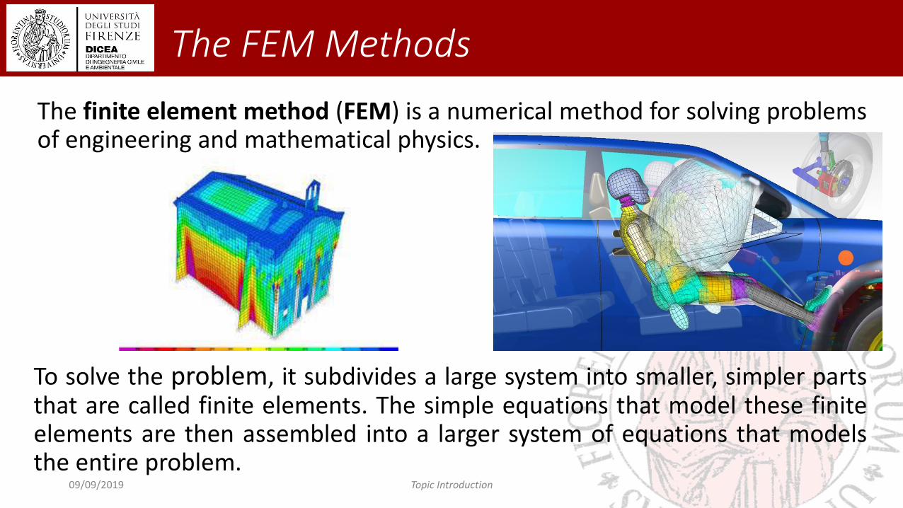
The finite element method (FEM) is a numerical method for solving problems of engineering and mathematical physics.
The FEM Methods
09/09/2019 Topic Introduction
To solve the problem, it subdivides a large system into smaller, simpler partsthat are called finite elements. The simple equations that model these finiteelements are then assembled into a larger system of equations that modelsthe entire problem.

LS-DYNA is a general-purpose finite element program capable of simulatingcomplex real world problems.
It is used by the automobile, aerospace, construction, military, manufacturing,and bioengineering industries. LS-DYNA is optimized for shared and distributedmemory Unix, Linux, and Windows based, platforms, and it is fully QA'd byLSTC. The code's origins lie in highly nonlinear, transient dynamic finite elementanalysis using explicit time integration.
LS DYNA Software

Nonlinear• Changing boundary conditions (such as contact between parts that changes
over time);
• Large deformations (for example the crumpling of sheet metal parts);
• Nonlinear materials that do not exhibit ideally elastic behavior (for example thermoplastic polymers).
LS DYNA Software
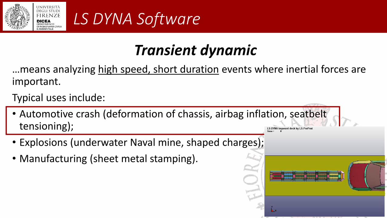
Transient dynamic…means analyzing high speed, short duration events where inertial forces are important.
Typical uses include:
• Automotive crash (deformation of chassis, airbag inflation, seatbelt tensioning);
• Explosions (underwater Naval mine, shaped charges);
• Manufacturing (sheet metal stamping).
LS DYNA Software

Need and characteristics: It is appropriate to investigate and solve problems characterized by:
• large deformations;
• sophisticated material models;
• complex contact conditions (with the possibility of automatically managing the contact areas); and
• working in time domain;
• modelling a wide range of material and their behaviour;
• models different types of elements.
LS DYNA Software

Main issues to be consider: • Complexity of the physical phenomenon;
• Interaction between multiple objects contacts, connections and penetration;
• Material behaviour according to the speed of the system;
• Secondary effects due to the application of "loads" (speed, forces, forcing, etc.).
LS DYNA Software
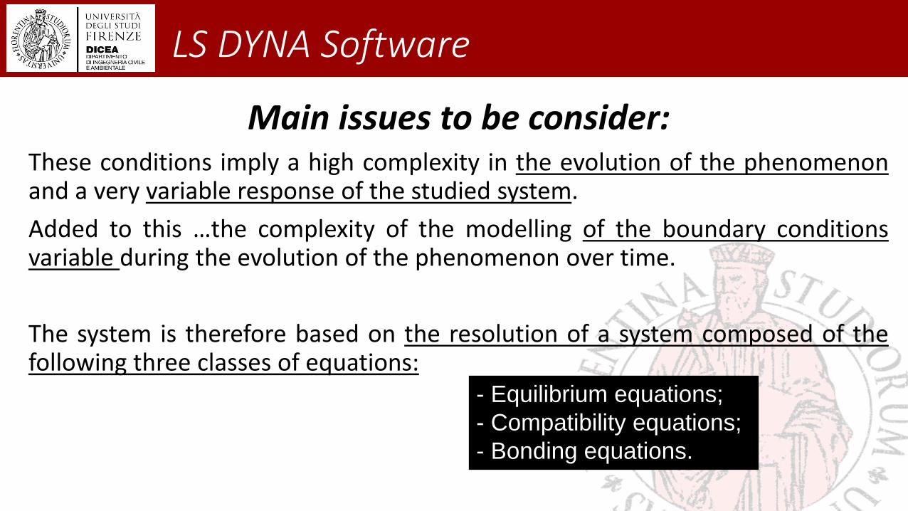
Main issues to be consider: These conditions imply a high complexity in the evolution of the phenomenonand a very variable response of the studied system.
Added to this …the complexity of the modelling of the boundary conditionsvariable during the evolution of the phenomenon over time.
The system is therefore based on the resolution of a system composed of thefollowing three classes of equations:
LS DYNA Software
- Equilibrium equations;
- Compatibility equations;
- Bonding equations.

Equilibrium equations:
LS DYNA Software
ሻ𝑀 ሷ𝑢 𝑡 + 𝐶 ሶ𝑢 𝑡 + 𝐾 𝑢 𝑡 = 𝑓(𝑡
Where [M], [C] and [K] are the matrix of masses, damping and elasticity respectively.
The three vectors represent velocity and acceleration displacements respectively.
Equilibrium equations relate stresses to applied forces.Hp: linear equations for small displacements
ሻ𝐾 𝑢 𝑡 = 𝑓(𝑡 Static analysis
Compatibility equations:
LS DYNA Software
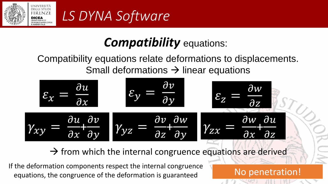
𝜀𝑥 =𝜕𝑢
𝜕𝑥
from which the internal congruence equations are derived
Compatibility equations relate deformations to displacements.
Small deformations linear equations
𝜀𝑦 =𝜕𝑣
𝜕𝑦 𝜀𝑧 =𝜕𝑤
𝜕𝑧
𝛾𝑥𝑦 =𝜕𝑢
𝜕𝑥+𝜕𝑣
𝜕𝑦𝛾𝑦𝑧 =
𝜕𝑣
𝜕𝑧+𝜕𝑤
𝜕𝑦𝛾𝑧𝑥 =
𝜕𝑤
𝜕𝑥+𝜕𝑢
𝜕𝑧
If the deformation components respect the internal congruence equations, the congruence of the deformation is guaranteed No penetration!

Bonding equations:
LS DYNA Software
Where ε, ሶ𝜀 represent the deformation of the material and its velocity deformation.
The binding equations describe a constitutive empirical relationship
that can be of various types…(elastic, elastic-plastic, thermal…)
𝜎 = 𝑓(𝜀, ሶሻ𝜀

LS DYNA Software
ሻ𝑀 ሷ𝑢 𝑡 + 𝐶 ሶ𝑢 𝑡 + 𝐾 𝑢 𝑡 = 𝑓(𝑡 ሻ𝑀 ሷ𝑢 𝑡 + 𝐶 ሶ𝑢 𝑡 + ሻ𝐾(𝑢 𝑢 𝑡 = 𝑓(𝑡
The analytical solution of the "linear" case
is available in a closed form
Of more interest is the resolution of the "non-linear" case,
that is when, at each integration step, the matrices can
change (being a function of time)
- Implicit methods;
- Explicit methods.Newmark
iterative numerical integration methods

LS DYNA Software
explicit codes generally based on the central differences methods.
The equations of equilibrium at the nodes are written in the configuration for
which both the displacement and the speed are already known, so that once
the acceleration has been calculated, it is possible to proceed with integration
over time.
ሻ𝑢𝑛+1 = 𝑢𝑛 + ∆𝑡 × 𝑓(𝑢𝑛, 𝑡𝑛The solution to a generic time does not depend on itself,
but only on the solution at the previous instant.
The most used method of this type is the integration of finite differences.
LS DYNA Software
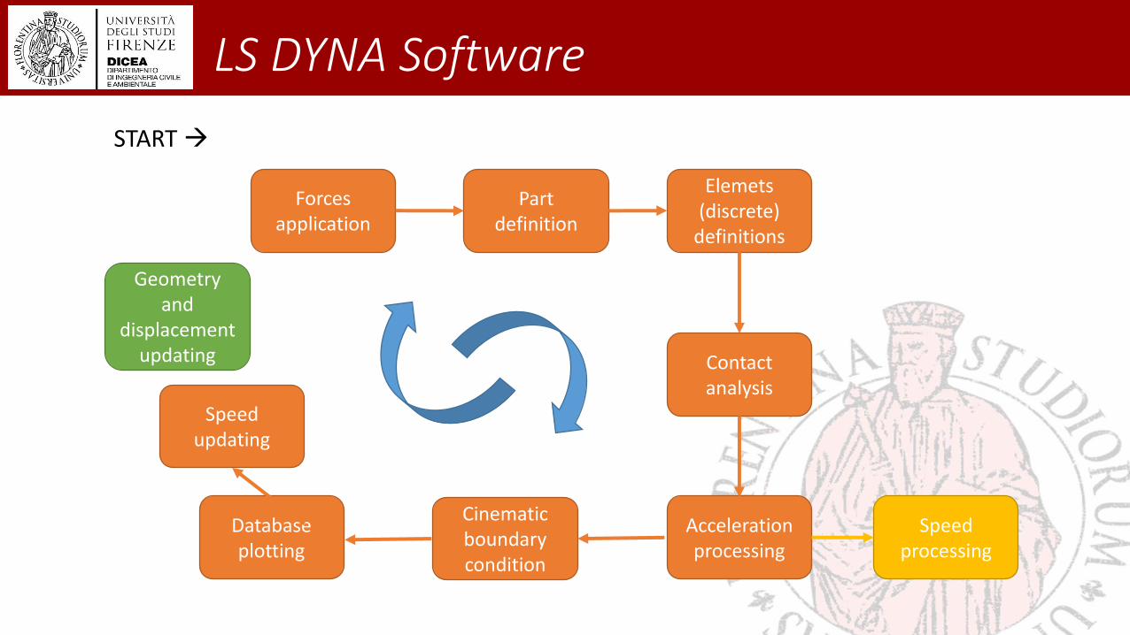
START
Forcesapplication
Part definition
Elemets(discrete)
definitions
Contactanalysis
Acceleration processing
Speedprocessing
Cinematicboundarycondition
Database plotting
Speedupdating
Geometryand
displacementupdating

LS DYNA Software
Eliminating the problem of
having to invert stiffness
matrix at each step; in
addition the equations are
decoupled and can
therefore be solved directly
without recourse to
convergence checks.
The method work with very
small integration intervals,
which therefore quickly
increase the computational
cost in determining the
solution, obviously seeking to
achieve a sufficient accuracy.

LS DYNA Software
The main problem, in using an explicit solver like LS-DYNA in the
analysis of crash phenomena, is the optimization of the three following factors:
- Accuracy;
- Calculation time;
- Stability.
Accuracy
Calculation time
Stability of the solution
Definition of the “time step”
LS DYNA Software
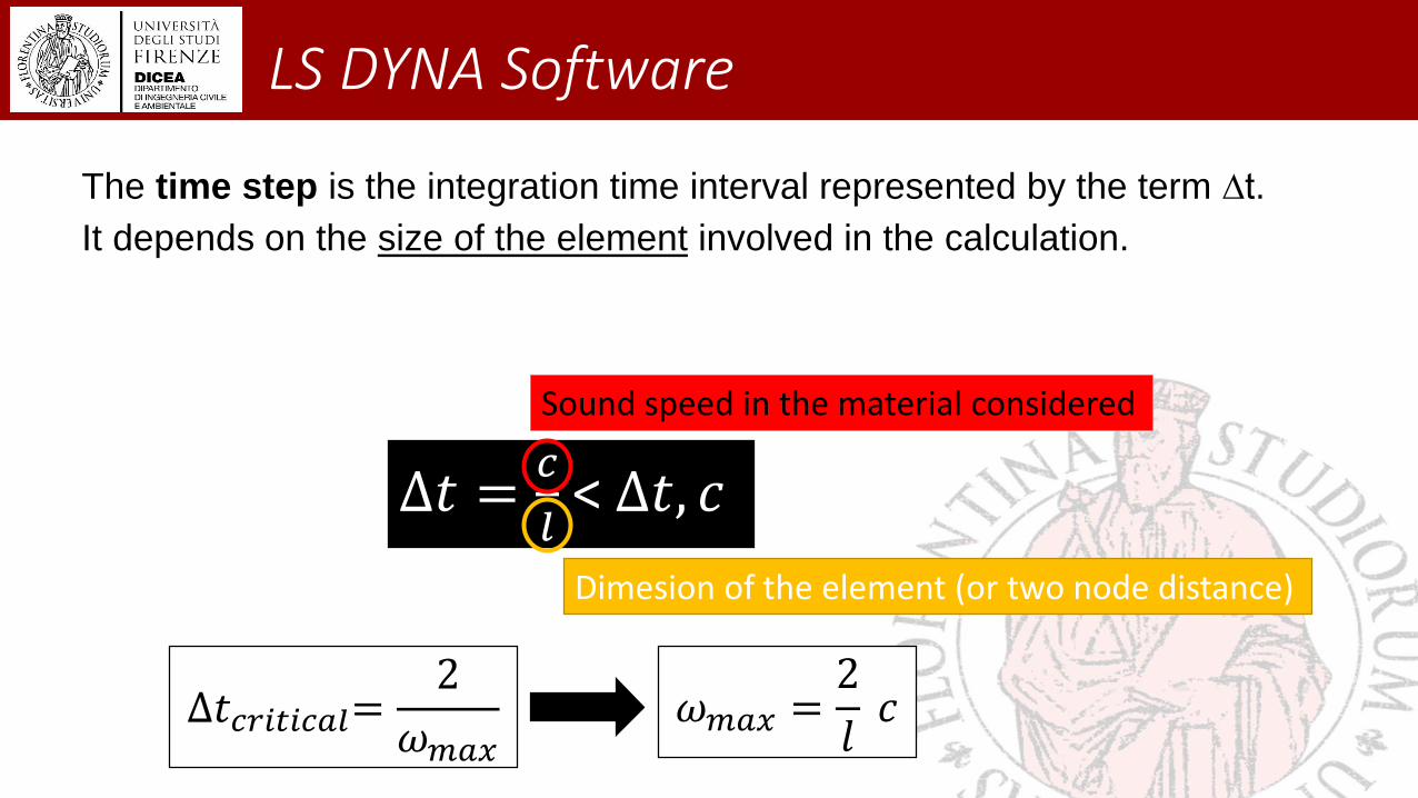
The time step is the integration time interval represented by the term ∆t.
It depends on the size of the element involved in the calculation.
∆𝑡 =𝑐
𝑙< ∆𝑡, 𝑐
Sound speed in the material considered
Dimesion of the element (or two node distance)
∆𝑡𝑐𝑟𝑖𝑡𝑖𝑐𝑎𝑙=2
𝜔𝑚𝑎𝑥𝜔𝑚𝑎𝑥 =
2
𝑙𝑐

LS DYNA Software
Pre-processing
Analysis
Post-processing

LS DYNA Software
Pre-processingFE modeling
Definition of the geometry
FEM characterization
Assembly of the different parts

LS DYNA Software
Pre-processingDefinition of the geometry
Construction of the 3D model/models
Surface
modelingMid surface

LS DYNA Software
Pre-processingFEM characterization
*part
Hierarchical approach
*mat*section
database
LS DYNA Software
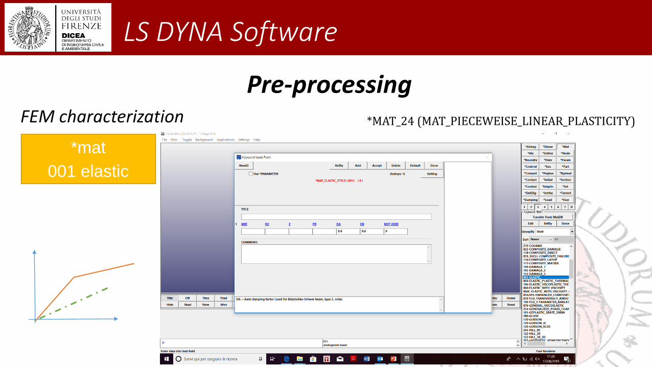
Pre-processingFEM characterization
*mat
001 elastic
*MAT_24 (MAT_PIECEWEISE_LINEAR_PLASTICITY)

LS DYNA Software
Pre-processingFEM characterization
*section
Type of element and # of integrationpoint

LS DYNA Software
Pre-processingFEM characterization
*part
*mat*section
Connection between
different parts of the
model..and with the
environment

LS DYNA Software
Pre-processingFEM characterization
Connection between
different parts of the
model
C/B analysis
will be
conducted
# and dimensions of the elements computational cost and findings

LS DYNA Software
Pre-processingFEM characterization
different components but the same material
as if they were welded1-D elements characterized by the same property
of the bolts

LS DYNA Software
Pre-processingFEM characterization
1) Soil modelling solid element in order to reproduce the real effect

LS DYNA Software
Pre-processingFEM characterization
1) Soil modelling solid element in order to reproduce the real effect

LS DYNA Software
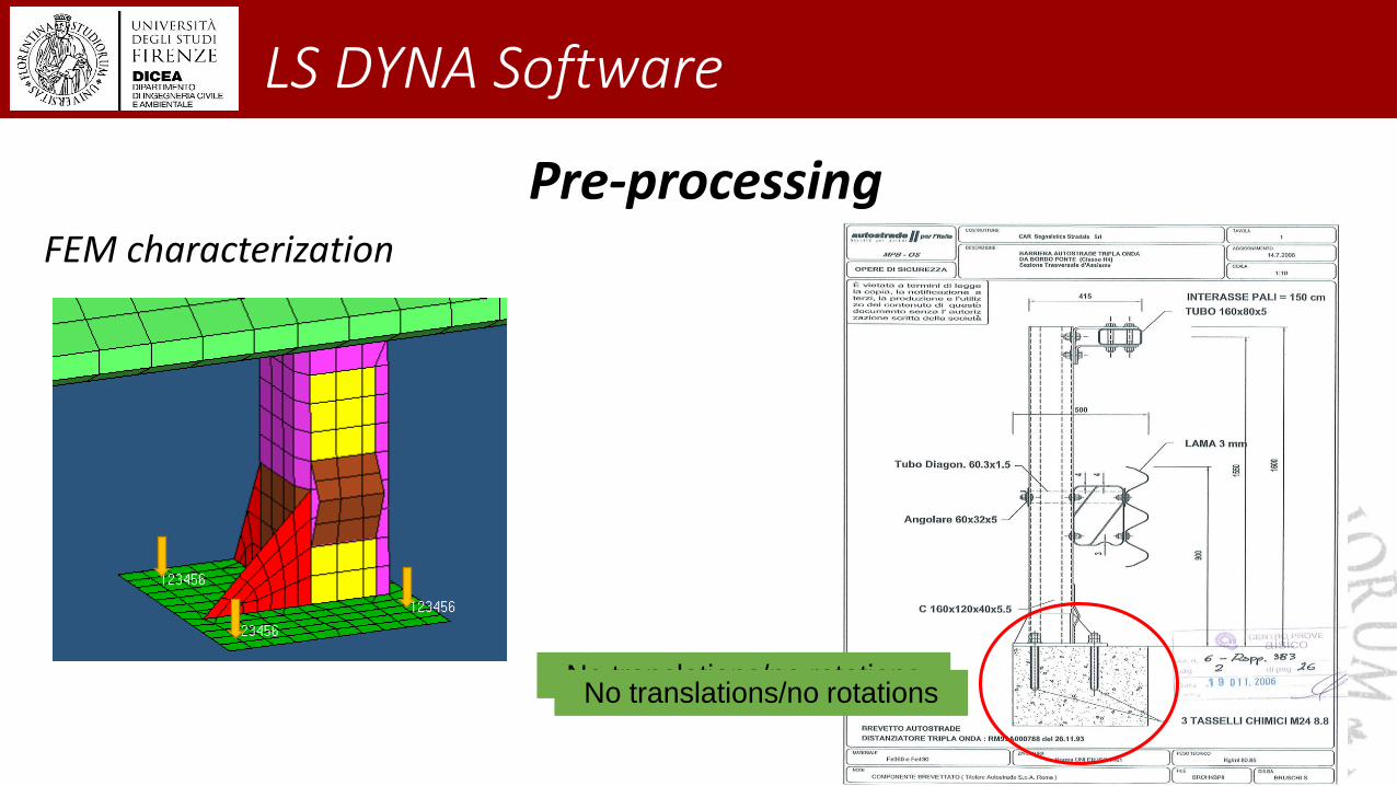
Pre-processingFEM characterization
2) Definition of boundary condition
6 DoF x,y,z directions and 3 rotations

LS DYNA Software
Pre-processingFEM characterization
2) Definition of boundary condition
6 DoF x,y,z directions and 3 rotations
LS DYNA Software
No translations/no rotations
Pre-processingFEM characterization
No translations/no rotations

LS DYNA Software
Pre-processingFEM characterization
…and what are the BCs at the end of the barrier? how
is the terminal modeled?
K
The selection of the type of BCs depends:
1) from the behaviour of the barrier during the crash
test;
2) from the behaviour of the barrier during the
accident.
the total length of the device also affects the selection
of the constraint

LS DYNA Software
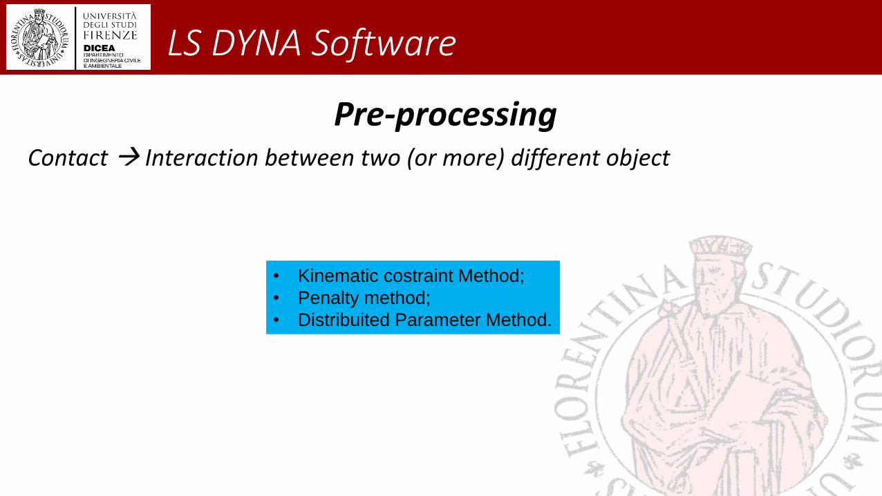
Pre-processingContact Interaction between two (or more) different object
contact management is necessary both to represent
the crash phenomena and to represent the interaction
between two parts of the same "object"
Implicit VS Explicit
high simplicity of
contact setup
ANSYS LS DYNA
LS DYNA Software
Pre-processingContact Interaction between two (or more) different object
• Kinematic costraint Method;
• Penalty method;
• Distribuited Parameter Method.

LS DYNA Software
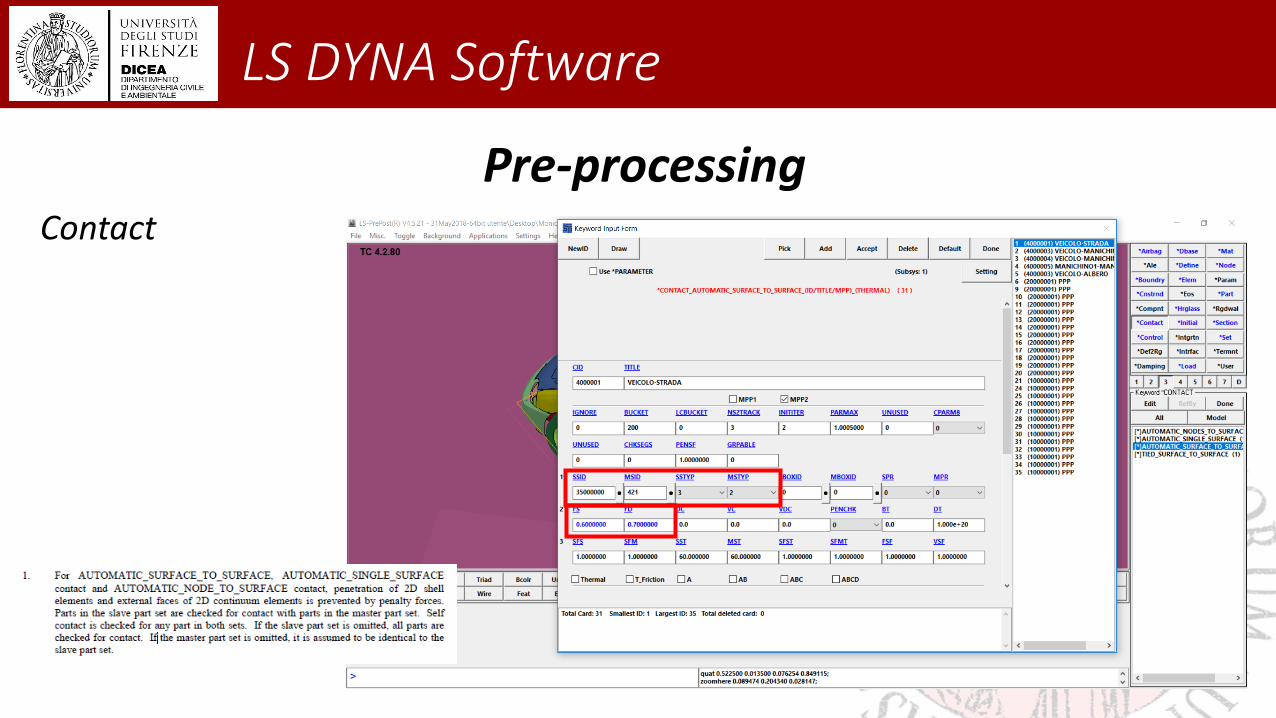
Pre-processingContact Penalty methods
1. Contact Search;
2. Contact Orientation;
3. Offset of the affected surfaces;
4. Contact Stiffness.
Main contact used for the reproduction of the crash phenomena
slave
master

LS DYNA Software
Pre-processingContact search
Practically , after the user has chosen the
elements involved in the contact, the solver
builds a grid and verify the distance between
each element of the grid separately, without
considering those that are far apart.
slave
master
Advantages: reduction of computational cost
LS DYNA Software
Pre-processingContact
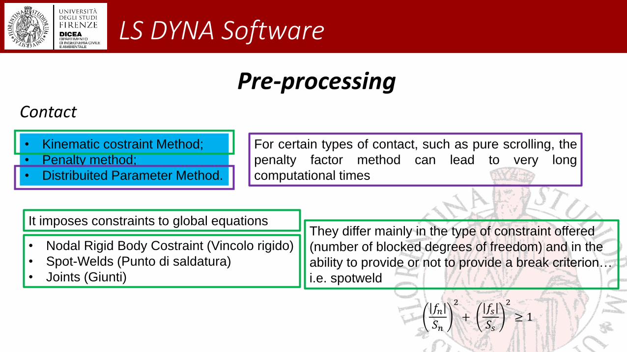
• Kinematic costraint Method;
• Penalty method;
• Distribuited Parameter Method.
For certain types of contact, such as pure scrolling, the
penalty factor method can lead to very long
computational times
It imposes constraints to global equations
• Nodal Rigid Body Costraint (Vincolo rigido)
• Spot-Welds (Punto di saldatura)
• Joints (Giunti)
They differ mainly in the type of constraint offered
(number of blocked degrees of freedom) and in the
ability to provide or not to provide a break criterion…
i.e. spotweld
𝑓𝑛𝑆𝑛
2
+𝑓𝑠𝑆𝑠
2
≥ 1
LS DYNA Software
Pre-processingContact

LS DYNA Software
Pre-processing*Initial …velocity
*Define curve…
LS DYNA Software
…and practically….