Road Infrastructure and Enterprise Development in Ethiopia

Admasu Shiferaw (The College of William and Mary)

With

Mans Söderbom, Eyerusalem Siba and Getnet Alemu

Introduction • Poor infrastructure and high transport costs pose a major

constraint to economic growth (Bloom and Sachs, 1998)

• Problem particularly stifling for manufacturing (Collier, 2000)

• It also explains why firms in low-income countries are born small and remain small (Tybout, 2000)

• These descriptions portray the situation in SSA where infrastructure is typically poor and manufacturing is dominated by small and micro-enterprises

Introduction • However, the role of infrastructure on the distribution/

behavior of manufacturing firms in Africa remains widely unknown – although the returns are supposedly higher

• Firms’ response to infrastructural capital is well documented in developed countries (Arauzo et al. 2010)

• There are a few recent studies on emerging countries (Chen, 1996; Datta 2011; Baum-Snow 2012)

• Similar studies in Africa only focus on rural households (Dercon et al., 2008; Renkow et al., 2004)

The Ethiopian Case • Ethiopia shares most of the challenges of SSA countries

– Landlocked since the secession of Eritrea in 1993 – Literally no railway systems and non-navigable rivers – Heavily dependent on road infrastructure

• Ethiopia has undertaken a massive Road Sector Development Program(RSDP) since 1997 – Three RSDPs impemented during 1997-2001; 2002-2007; 2008-2010 – Total cost more than $7.00 billion – Funded party by international donors – Already shows great improvement

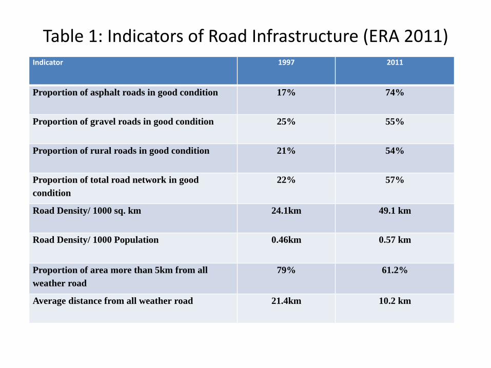
Table 1: Indicators of Road Infrastructure (ERA 2011) Indicator 1997 2011

Proportion of asphalt roads in good condition 17% 74%

Proportion of gravel roads in good condition 25% 55%

Proportion of rural roads in good condition 21% 54%

Proportion of total road network in good condition

22% 57%

Road Density/ 1000 sq. km 24.1km 49.1 km

Road Density/ 1000 Population 0.46km 0.57 km

Proportion of area more than 5km from all weather road

79% 61.2%

Average distance from all weather road 21.4km 10.2 km

Objective of the Paper • Assess the response of Ethiopian manufacturing

firms to the improved road networks:

• Key questions: 1. Does improvement in road networks make towns more

attractive for manufacturing firms? In other words, does the RSDP influcence firms‘ location choices?

2. Has the start-up size of manufacturing firms increased due to better road networks?

Declining Share of Top Five Towns in Manufacturing Firms

0.0

0.5

1.0

1.5

2.0

2.5

3.0

3.5

4.0

4.5

0.0

10.0

20.0

30.0

40.0

50.0

60.0

70.0

80.0

90.0

1996 1997 1998 1999 2000 2001 2002 2003 2004 2005 2006 2007 2008 2009

Addi

s Aba

b a

nd T

op F

ive

Addis Ababa Top Five Dire Dawa

Town and Firm Level Panel Data • The empirical work combines two data sources:

– GIS based town level panel data on road accessibility – Firm level panel data from Ethiopian manufacturing

• The GIS data is from the Ethiopian Roads Authority (ERA). – Geo-coded project level data on roads – Detailed indicators on project status (rehabilitation, upgrading and

construction of new roads) and type of pavement

• GIS analytical tools to measure road accessibility of towns:

– Service Coverage Analysis, and – Origin-Destination (OD) Matrix

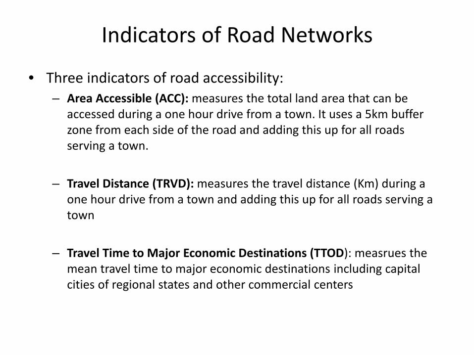
Indicators of Road Networks

• Three indicators of road accessibility: – Area Accessible (ACC): measures the total land area that can be

accessed during a one hour drive from a town. It uses a 5km buffer zone from each side of the road and adding this up for all roads serving a town.

– Travel Distance (TRVD): measures the travel distance (Km) during a one hour drive from a town and adding this up for all roads serving a town

– Travel Time to Major Economic Destinations (TTOD): measrues the mean travel time to major economic destinations including capital cities of regional states and other commercial centers

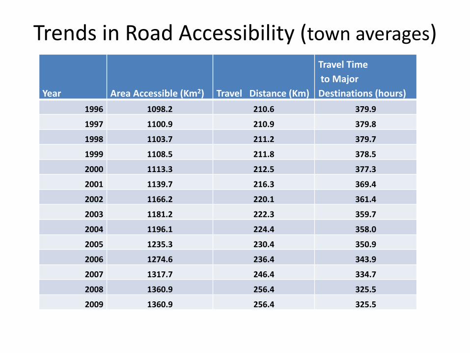
Trends in Road Accessibility (town averages)

Year Area Accessible (Km2) Travel Distance (Km)

Travel Time to Major Destinations (hours)

1996 1098.2 210.6 379.9

1997 1100.9 210.9 379.8

1998 1103.7 211.2 379.7

1999 1108.5 211.8 378.5

2000 1113.3 212.5 377.3

2001 1139.7 216.3 369.4

2002 1166.2 220.1 361.4

2003 1181.2 222.3 359.7

2004 1196.1 224.4 358.0

2005 1235.3 230.4 350.9

2006 1274.6 236.4 343.9

2007 1317.7 246.4 334.7

2008 1360.9 256.4 325.5

2009 1360.9 256.4 325.5

0

200

400

600

800

1000

1200

1400

1600

0

50

100

150

200

250

300

350

400

1996 1997 1998 1999 2000 2001 2002 2003 2004 2005 2006 2007 2008 2009

Trav

el D

ista

nce

and

Trav

el T

ime

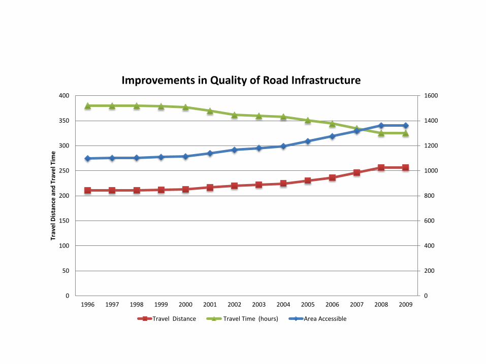
Improvements in Quality of Road Infrastructure

Travel Distance Travel Time (hours) Area Accessible

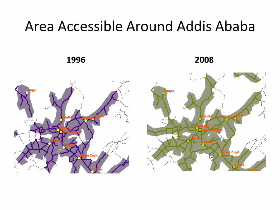
Area Accessible Around Addis Ababa

1996 2008

Firm Level Data • Census based firm level panel data from the Ethiopian Statistical

Agency (CSA)

• The census captures all firms that employ at least 10 workers and use power driven machinery. The number of firms increased from 610 in 1996 to 1713 in 2009.

• For the first research question, we calculate the total number of firms as well as the number of new firms in a town.

• For the second research question we examine the number of

workers of new firms as our dependent variable

• A firm is considered to be an entrant if it appears in the census for the first time

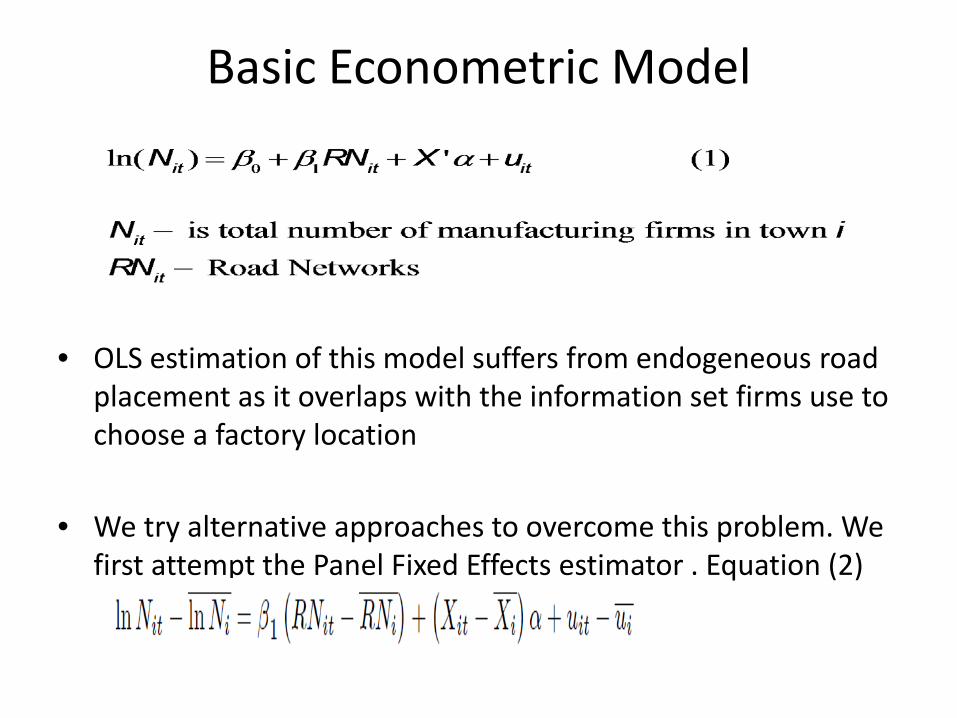
Basic Econometric Model

• OLS estimation of this model suffers from endogeneous road

placement as it overlaps with the information set firms use to choose a factory location

• We try alternative approaches to overcome this problem. We first attempt the Panel Fixed Effects estimator . Equation (2)

• The with-in estimator does not capture the dynamics of agglomeration effects and other sources of persistence in the number of firms in a town.

• To capture that we use the Blundel and Bond (1998) System GMM estimator which also uses internal instruments to address endogenous road placement. Equation (3):

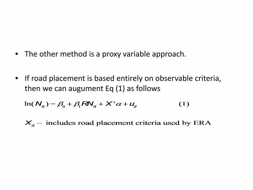
• The other method is a proxy variable approach.

• If road placement is based entirely on observable criteria, then we can augument Eq (1) as follows

ERA‘s Criteria for Road Placement • The process starts with submissions of proposals by regional

governments to ERA

• Priority in the assignment of new road projects is based on the following factors: – Economic development potentials (20%) – Surplus food and cash crop production (20%) – Roads that connect existing major roads (20%) – Large and isolated population centers (30%) – Balanced development among regions (10%)

• Lack of clarity on how these criteria are operationalized

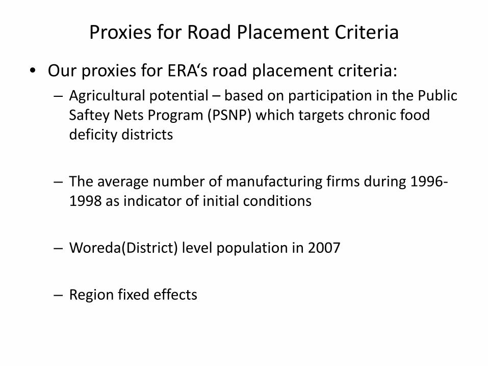
Proxies for Road Placement Criteria

• Our proxies for ERA‘s road placement criteria: – Agricultural potential – based on participation in the Public

Saftey Nets Program (PSNP) which targets chronic food deficity districts

– The average number of manufacturing firms during 1996-1998 as indicator of initial conditions

– Woreda(District) level population in 2007

– Region fixed effects

Results • We first present OLS estimates of partial correlations

using: – Average number of firms in a town during 1999-2009 as

the dependent variable – Average values of road accessibility during 1999-2009, and – Proxies for road placement – Data is cross-sectional b/c we are taking period averages

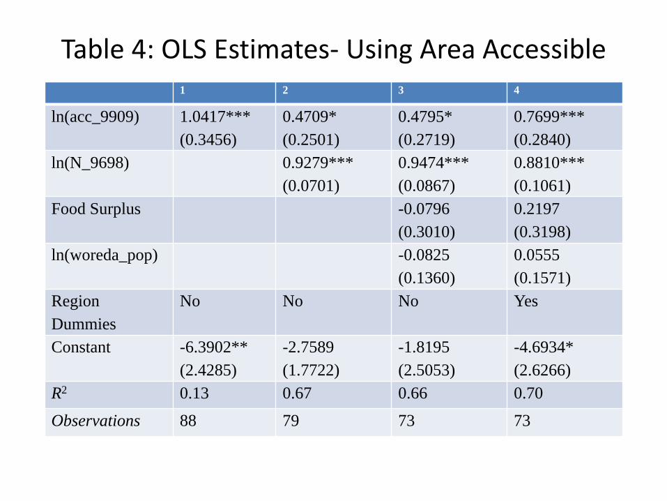
Table 4: OLS Estimates- Using Area Accessible 1 2 3 4

ln(acc_9909) 1.0417*** (0.3456)

0.4709* (0.2501)

0.4795* (0.2719)

0.7699*** (0.2840)

ln(N_9698) 0.9279*** (0.0701)

0.9474*** (0.0867)

0.8810*** (0.1061)

Food Surplus -0.0796 (0.3010)

0.2197 (0.3198)

ln(woreda_pop) -0.0825 (0.1360)

0.0555 (0.1571)

Region Dummies

No No No Yes

Constant -6.3902** (2.4285)

-2.7589 (1.7722)

-1.8195 (2.5053)

-4.6934* (2.6266)

R2 0.13 0.67 0.66 0.70

Observations 88 79 73 73

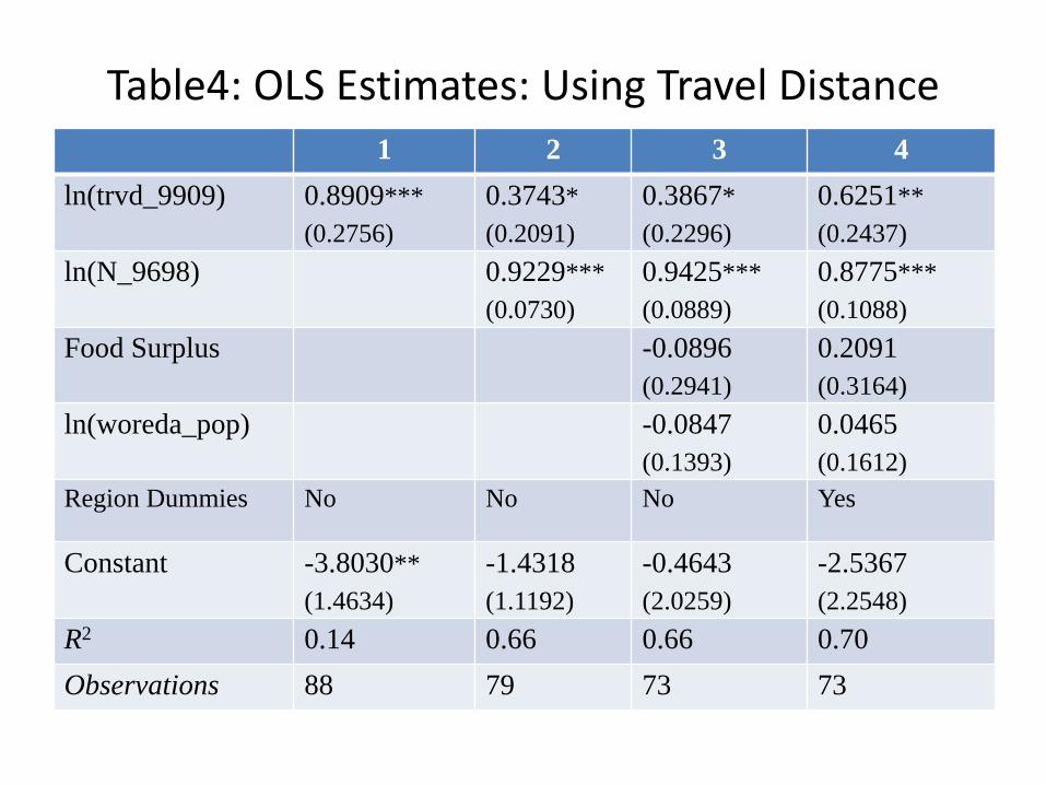
Table4: OLS Estimates: Using Travel Distance 1 2 3 4

ln(trvd_9909) 0.8909*** (0.2756)

0.3743* (0.2091)

0.3867* (0.2296)

0.6251** (0.2437)

ln(N_9698) 0.9229*** (0.0730)

0.9425*** (0.0889)

0.8775*** (0.1088)

Food Surplus -0.0896 (0.2941)

0.2091 (0.3164)

ln(woreda_pop) -0.0847 (0.1393)

0.0465 (0.1612)

Region Dummies No No No Yes

Constant -3.8030** (1.4634)

-1.4318 (1.1192)

-0.4643 (2.0259)

-2.5367 (2.2548)

R2 0.14 0.66 0.66 0.70 Observations 88 79 73 73

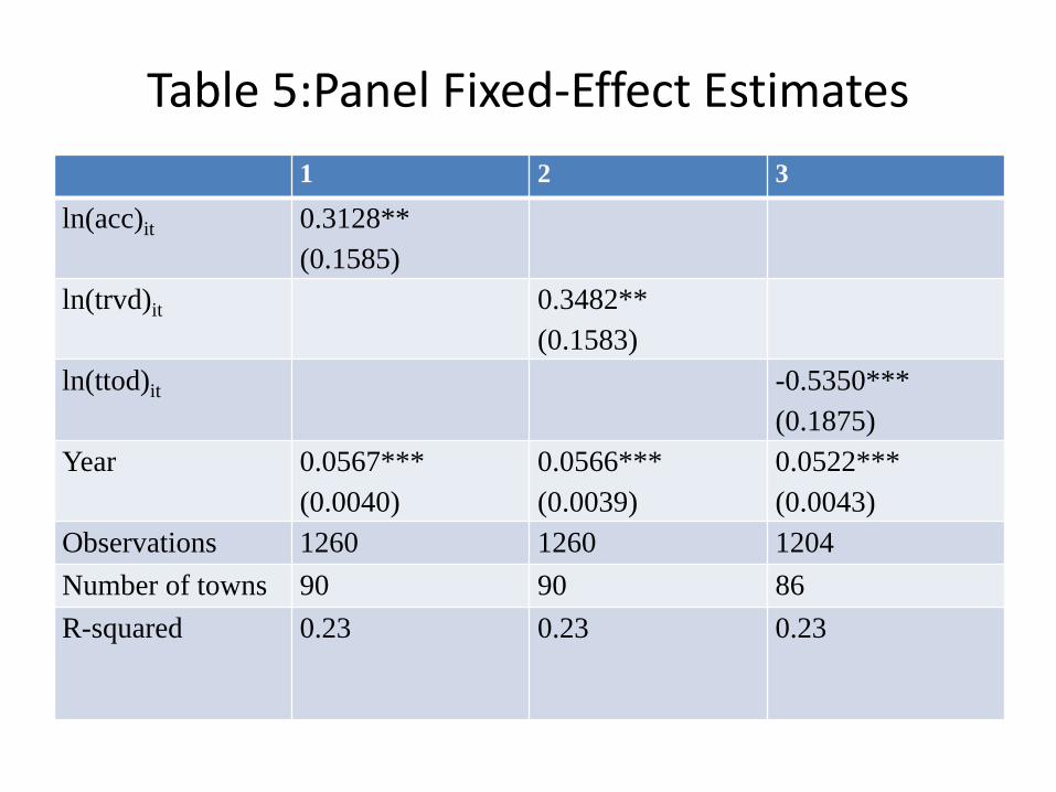
Table 5:Panel Fixed-Effect Estimates 1 2 3

ln(acc)it 0.3128** (0.1585)

ln(trvd)it 0.3482** (0.1583)

ln(ttod)it -0.5350*** (0.1875)

Year 0.0567*** (0.0040)

0.0566*** (0.0039)

0.0522*** (0.0043)

Observations 1260 1260 1204 Number of towns 90 90 86 R-squared 0.23 0.23 0.23

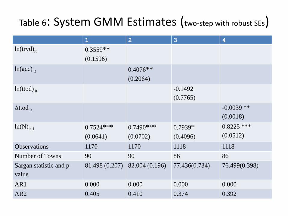
Table 6: System GMM Estimates (two-step with robust SEs) 1 2 3 4

ln(trvd)it 0.3559** (0.1596)

ln(acc) it 0.4076** (0.2064)

ln(ttod) it -0.1492 (0.7765)

∆ttod it -0.0039 ** (0.0018)

ln(N)it-1 0.7524*** (0.0641)

0.7490*** (0.0702)

0.7939* (0.4096)

0.8225 *** (0.0512)

Observations 1170 1170 1118 1118 Number of Towns 90 90 86 86 Sargan statistic and p-value

81.498 (0.207) 82.004 (0.196) 77.436(0.734) 76.499(0.398)

AR1 0.000 0.000 0.000 0.000 AR2 0.405 0.410 0.374 0.392

Number of Entrants as a Response Variable • The previous analysis conflates survival of incumbents and

firm entry

• In this section we focus only on gross firm entry in a town • Since the number of new firms in a town per annum is

relatively small we use Count Data Models (Poisson).

• However, due to the restrictive assumptions of the Poisson estimator and the prevalence of zero entrants in most towns, we use the Zero Inflated Negative Binomial Model.

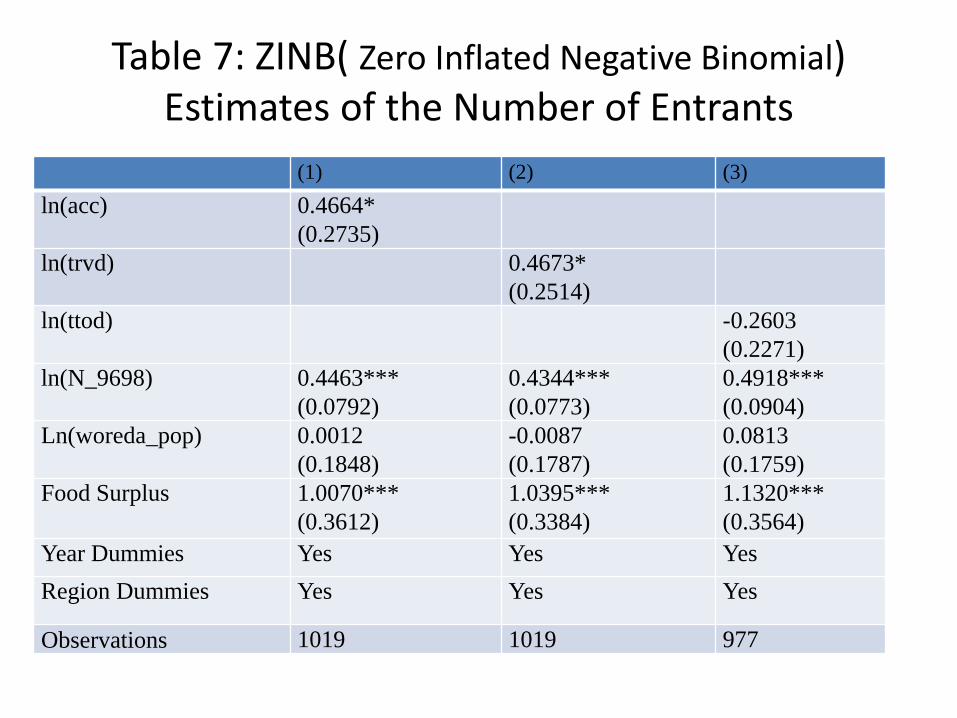
Table 7: ZINB( Zero Inflated Negative Binomial) Estimates of the Number of Entrants

(1) (2) (3) ln(acc)

0.4664* (0.2735)

ln(trvd)

0.4673* (0.2514)

ln(ttod)

-0.2603 (0.2271)

ln(N_9698)

0.4463*** (0.0792)

0.4344*** (0.0773)

0.4918*** (0.0904)

Ln(woreda_pop)

0.0012 (0.1848)

-0.0087 (0.1787)

0.0813 (0.1759)

Food Surplus

1.0070*** (0.3612)

1.0395*** (0.3384)

1.1320*** (0.3564)

Year Dummies Yes Yes Yes Region Dummies Yes Yes Yes

Observations 1019 1019 977

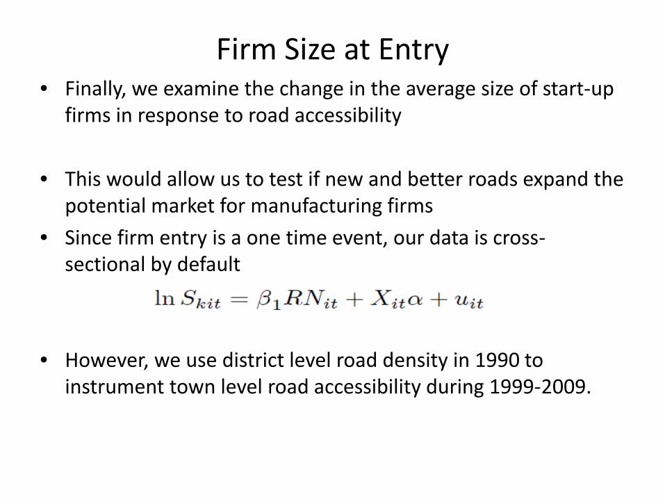
Firm Size at Entry • Finally, we examine the change in the average size of start-up

firms in response to road accessibility

• This would allow us to test if new and better roads expand the potential market for manufacturing firms

• Since firm entry is a one time event, our data is cross-sectional by default

• However, we use district level road density in 1990 to instrument town level road accessibility during 1999-2009.

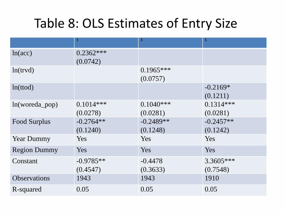
Table 8: OLS Estimates of Entry Size 1 3 5

ln(acc) 0.2362*** (0.0742)

ln(trvd) 0.1965*** (0.0757)

ln(ttod) -0.2169* (0.1211)

ln(woreda_pop) 0.1014*** (0.0278)

0.1040*** (0.0281)

0.1314*** (0.0281)

Food Surplus -0.2764** (0.1240)

-0.2489** (0.1248)

-0.2457** (0.1242)

Year Dummy Yes Yes Yes Region Dummy Yes Yes Yes Constant -0.9785**

(0.4547) -0.4478 (0.3633)

3.3605*** (0.7548)

Observations 1943 1943 1910 R-squared 0.05 0.05 0.05

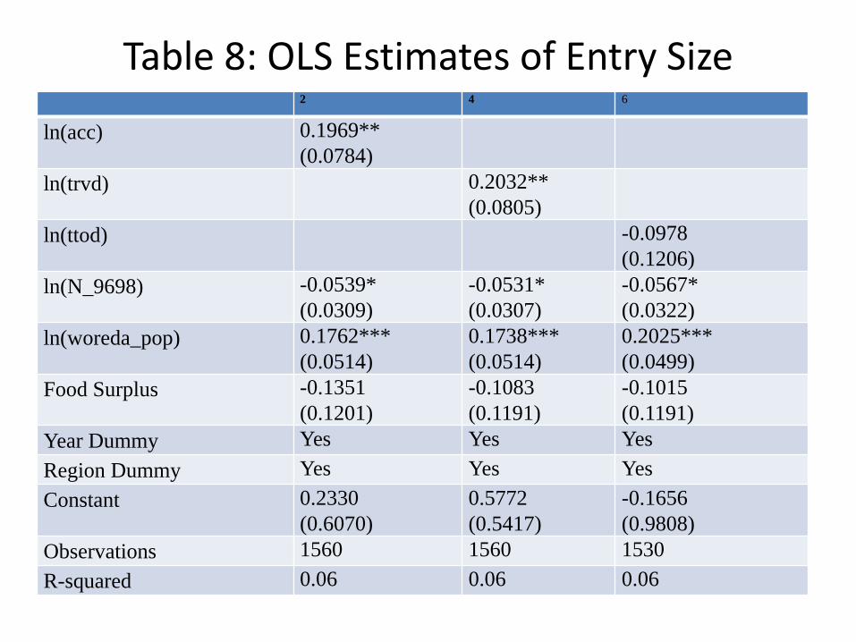
Table 8: OLS Estimates of Entry Size 2 4 6

ln(acc) 0.1969** (0.0784)

ln(trvd) 0.2032** (0.0805)

ln(ttod) -0.0978 (0.1206)

ln(N_9698) -0.0539* (0.0309)

-0.0531* (0.0307)

-0.0567* (0.0322)

ln(woreda_pop) 0.1762*** (0.0514)

0.1738*** (0.0514)

0.2025*** (0.0499)

Food Surplus -0.1351 (0.1201)

-0.1083 (0.1191)

-0.1015 (0.1191)

Year Dummy Yes Yes Yes Region Dummy Yes Yes Yes Constant 0.2330

(0.6070) 0.5772 (0.5417)

-0.1656 (0.9808)

Observations 1560 1560 1530 R-squared 0.06 0.06 0.06

Table 9: 2SLS Estimates of Entry Size 1 2 3

ln(acc)

0.3619* (0.1965)

ln(trvd)

0.4022* (0.2238)

ln(ttod)

-1.0849* (0.5687)

ln(N_9698)

-0.0440 (0.0323)

-0.0392 (0.0332)

0.0144 (0.0527)

ln(woreda_pop)

0.1498** (0.0598)

0.1387** (0.0642)

0.1458** (0.0635)

Food Surplus

-0.1723 (0.1247)

-0.1346 (0.1189)

-0.1297 (0.1181)

Year Dummy Yes Yes Yes Region Dummy Yes Yes Yes Constant

-2.1228** (0.8359)

-1.5093** (0.6015)

6.4142* (3.8764)

Observations 1474 1474 1474

Conclusions • The RSDP has increased road networks significantly across

towns in Ethiopia

• While the number of manufacturing firms has increased during the sample period, the rate of entry is higher for towns with better road networks

• Historical centres of manufacturing still remain competitive and attractive. However, the RSDP has began to reduce the geographic concentration of manufacturing

• The RSDP has also improved the average size of business start-ups – which has positive implications on firm survival and growth