RNA sequencing for the study of gene expression regulation · PDF fileRNA sequencing for the...
193
RNA sequencing for the study of gene expression regulation ˆ Angela Teresa Filimon Gon¸calves European Bioinformatics Institute Darwin College A thesis submitted to the University of Cambridge for the degree of Doctor of Philosophy September 2012
-
Upload
hoangkhanh -
Category
Documents
-
view
235 -
download
6
Transcript of RNA sequencing for the study of gene expression regulation · PDF fileRNA sequencing for the...

RNA sequencing for the study of
gene expression regulation
Angela Teresa Filimon Goncalves
European Bioinformatics Institute
Darwin College
A thesis submitted to the University of Cambridge for the degree of
Doctor of Philosophy
September 2012


Declaration of Originality
This thesis is the result of my own work and includes nothing which
is the outcome of work done in collaboration except where specifically
indicated in the text.
The text in this thesis does not exceed the limit of 60,000 words set by
the Biology Degree Committee.

RNA sequencing for the study of gene expression regulation
Angela Teresa Filimon GoncalvesSummary
The process by which information encoded in an organism’s DNA is
used in the synthesis of functional cell products is known as gene ex-
pression. In recent years, sequencing of RNA (RNA-seq) has emerged as
the preferred technology for the simultaneous measurement of transcript
sequences and their abundance.
The analysis of RNA-seq data presents novel challenges and many meth-
ods have been developed for the purpose of mapping reads to genomic
features and expression quantification. In the first part of my thesis I
developed an R based pipeline for pre-processing, expression estimation
and data quality assessment of RNA-seq datasets, which formed the ba-
sis for my subsequent work on the evolution of gene expression regulation
in mammals.
Since changes in gene expression levels are thought to underlie many
of the phenotypic differences between species, identifying and charac-
terising the regulatory mechanisms responsible for these changes is an
important goal of molecular biology. For this, I studied the regulatory
divergence of liver gene expression and of isoform usage between mouse
strains. I demonstrate that gene expression diverges extensively between
the strains and propose that the regulatory mechanism underlying di-
vergent expression between two closely related mammalian species is a
combination of variants that arise in cis and in trans. Isoform usage
diverges to a lesser extent and appears to display a larger contribution
of trans acting regulatory elements to its regulation, suggesting that
isoform usage may be under different evolutionary constraints. These
observations have important implications for understanding mammalian
gene expression divergence and for understanding how speciation occurs.


Acknowledgements
This work was carried out in the Functional Genomics Group at the Eu-
ropean Bioinformatics Institute and was funded by the European Molec-
ular Biology Laboratory.
I would like to thank my supervisor Alvis Brazma for his support over
these years. I am very grateful for his guidance, openness and positivity.
I am also indebted to Wolfgang Huber, for his excellent advice, and
to Duncan Odom and Paul Flicek, who have allowed me to be part
of the great FOG team. Their knowledge and enthusiasm have been
most invaluable and inspiring. Thanks also to Sarah Leigh-Brown, Klara
Stefflova and David Thybert for generously sharing their knowledge with
me and for all the stimulating and fun meetings we have had.
I can not thank John Marioni enough for his outstanding support, in
particular of the work described in the last two chapters of this thesis. It
has been a great pleasure working with him. I am also indebted to John,
Ernest Turro, Petra Schwalie and Nenad Bartonicek for their valuable
comments and for proofreading this thesis.
My thanks to all the Functional Genomics Group members, in partic-
ular to Mar Gonzalez-Porta, Gabriella Rustici and Johan Rung for all
the helpful discussions, Mar and Gabriella for their companionship in
teaching bioinformatics around the world and Lynn French for greatly
facilitating my life with travel and bureaucratic support.
I have been fortunate to have spent my time at the EBI among an ex-
traordinary group of fellow PhD students and Postdocs. They have
all enriched my life and made my stay here unforgettable. A spe-
cial thanks to Nenad Bartonicek, Anika Oellrich, Andre Faure, Steven
Wilder, Mikhail Spivakov, Joseph Foster and Tim Wiegels, who have
been there from the beginning. Mostly, I want to thank Petra Schwalie
with whom it is the greatest pleasure to discuss work, life and just about
anything. She has become a dear friend.


Looking back into the past, this thesis would not have happened without
my master’s thesis supervisor Ernesto Costa, who got me interested in
gene expression regulation in the first place. I hope he enjoys reading
this work!
Finally, I thank my amazing parents, who have always done so much
for me, and Ernest Turro, who has patiently supported me and made
numerous contributions to my work throughout.


Contents
Contents x
1 Introduction 1
1.1 The regulation of gene expression . . . . . . . . . . . . . . . . . . . . 2
1.1.1 Regulation of transcription initiation . . . . . . . . . . . . . . 3
1.1.2 Transcript elongation control . . . . . . . . . . . . . . . . . . 4
1.1.3 Regulation by chromatin structure and DNA methylation . . . 5
1.1.4 Regulation of RNA processing . . . . . . . . . . . . . . . . . 9
1.1.5 Regulation of RNA degradation . . . . . . . . . . . . . . . . . 14
1.1.6 RNA editing . . . . . . . . . . . . . . . . . . . . . . . . . . . . 16
1.2 Sequence divergence to phenotypic divergence . . . . . . . . . . . . . 18
1.2.1 DNA sequence divergence . . . . . . . . . . . . . . . . . . . . 18
1.2.2 Gene regulatory divergence . . . . . . . . . . . . . . . . . . . 19
1.3 Measuring gene expression with RNA sequencing . . . . . . . . . . . 22
1.3.1 RNA sequencing experiment workflow . . . . . . . . . . . . . 23
1.3.2 Read mapping strategies . . . . . . . . . . . . . . . . . . . . . 25
1.3.3 Expression quantification . . . . . . . . . . . . . . . . . . . . . 32
1.3.4 Expression normalisation . . . . . . . . . . . . . . . . . . . . . 35
1.3.5 Differential expression . . . . . . . . . . . . . . . . . . . . . . 40
2 An RNA-seq analysis pipeline 43
2.1 Introduction . . . . . . . . . . . . . . . . . . . . . . . . . . . . . . . . 44
2.2 Methods . . . . . . . . . . . . . . . . . . . . . . . . . . . . . . . . . . 45
2.2.1 The analysis pipeline . . . . . . . . . . . . . . . . . . . . . . . 45
2.2.2 R cloud usage and analysis of public data . . . . . . . . . . . 48
x

CONTENTS
2.3 Discussion . . . . . . . . . . . . . . . . . . . . . . . . . . . . . . . . . 49
3 Compensatory cis and trans regulation dominates the evolution of
mouse gene expression 51
3.1 Introduction . . . . . . . . . . . . . . . . . . . . . . . . . . . . . . . . 52
3.2 Results . . . . . . . . . . . . . . . . . . . . . . . . . . . . . . . . . . . 55
3.2.1 Allele specific expression estimates can be obtained for 30%
of annotated mouse genes . . . . . . . . . . . . . . . . . . . . 56
3.2.2 Approximately a quarter of genes are differentially expressed
between C57BL/6J and CAST/EiJ . . . . . . . . . . . . . . . 58
3.2.3 Expression levels of circadian rhythm genes varies widely . . . 58
3.2.4 The identification of imprinted genes is strengthened by mul-
tiple replicates . . . . . . . . . . . . . . . . . . . . . . . . . . . 61
3.2.5 Most gene expression divergence is caused by a combination
of cis and trans regulatory variants . . . . . . . . . . . . . . . 64
3.2.6 Genes with regulatory divergence in trans show stronger se-
quence constraint . . . . . . . . . . . . . . . . . . . . . . . . . 69
3.3 Discussion . . . . . . . . . . . . . . . . . . . . . . . . . . . . . . . . . 71
3.3.1 Phenotypic diversity and intra-species heterogeneity in expres-
sion . . . . . . . . . . . . . . . . . . . . . . . . . . . . . . . . 73
3.3.2 A continuum of imprinting . . . . . . . . . . . . . . . . . . . . 74
3.3.3 Using the hybrid system to study the divergence of gene ex-
pression levels . . . . . . . . . . . . . . . . . . . . . . . . . . . 74
4 Decoupling of isoform and gene expression evolution in mice 78
4.1 Introduction . . . . . . . . . . . . . . . . . . . . . . . . . . . . . . . . 79
4.2 Results . . . . . . . . . . . . . . . . . . . . . . . . . . . . . . . . . . . 80
4.2.1 Isoform level estimates reveal complex patterns of imprinting . 84
4.2.2 Approximately 8% of genes have differential isoform usage be-
tween C57BL/6J and CAST/EiJ . . . . . . . . . . . . . . . . 87
4.2.3 Most isoform regulatory divergence is caused by regulatory
variants in trans . . . . . . . . . . . . . . . . . . . . . . . . . 90
4.3 Discussion . . . . . . . . . . . . . . . . . . . . . . . . . . . . . . . . . 93
xi

CONTENTS
5 Concluding remarks 100
A Supplementary material for Chapter 3 102
A.1 Experimental methods . . . . . . . . . . . . . . . . . . . . . . . . . . 102
A.1.1 Animal housing and handling . . . . . . . . . . . . . . . . . . 102
A.1.2 Sequencing library preparation . . . . . . . . . . . . . . . . . 103
A.1.3 Pyrosequencing . . . . . . . . . . . . . . . . . . . . . . . . . . 103
A.2 Supplementary Figures . . . . . . . . . . . . . . . . . . . . . . . . . . 105
A.3 Supplementary Tables . . . . . . . . . . . . . . . . . . . . . . . . . . 113
A.3.1 Supplementary Table A.1 . . . . . . . . . . . . . . . . . . . . 113
A.3.2 Supplementary Table A.2 . . . . . . . . . . . . . . . . . . . . 115
A.3.3 Supplementary Table A.3 . . . . . . . . . . . . . . . . . . . . 130
A.3.4 Supplementary Table A.4 . . . . . . . . . . . . . . . . . . . . 149
A.3.5 Supplementary Table A.5 . . . . . . . . . . . . . . . . . . . . 154
B Supplementary material for Chapter 4 155
B.1 Supplementary Figures . . . . . . . . . . . . . . . . . . . . . . . . . . 155
B.2 Supplementary Tables . . . . . . . . . . . . . . . . . . . . . . . . . . 157
B.2.1 Supplementary Table B.1 . . . . . . . . . . . . . . . . . . . . . 157
C Full list of publications 159
References 161
xii


Chapter 1
Introduction
The hereditary information of an eukaryotic organism is encoded in a genome com-
prising molecules of deoxyribonucleic acid (DNA) packed and organised in structures
called chromosomes. The information in a DNA molecule is represented by a se-
quence of smaller molecules called nucleotides containing one of four types of bases
(adenine - A, thymine - T, guanine - G or cytosine - C) and by other chemical
and structural features. Each DNA molecule is composed of two such sequences
known as strands held together by hydrogen bonds which can only form between
specific pairs of nucleotides: A with T and G with C. Because of this relationship
the two strands contain the same information and are said to be complementary to
one another.
Within a multicellular organism and throughout its life, its genome stays mostly
unchanged. In fact, almost all cells of an organism contain an almost exact copy of
the DNA that was in the fertilised egg from which the whole organism developed. Its
cells, however, can have very distinct appearances, functions and respond differently
to extracellular stimuli. These differences are possible because cells make different
use of stretches of the DNA, called genes, as templates to build functional cellular
products in a process called gene expression. The cellular products and their abun-
dance are the result of the integration of the present cell state and external signals
by a complex regulatory system which is itself encoded in the DNA sequence and
structure.
In the first step of gene expression, known as transcription, the information in
the DNA is used to create ribonucleic acid molecules (RNA). RNA is synthesised
1

using one of the DNA strands as a template and has the same chemical structure
except that thymine is replaced by uracil (U). Some RNA molecules can be the end
product in themselves and some can in turn be used as a template for the creation of
other molecules, proteins, in a process called translation. Proteins are composed of
one or more sequences of molecules called amino acids, each of which is determined
by an RNA nucleotide sequence in which each successive triplet corresponds to one
amino acid. According to this distinction between RNAs that are used as a template
for proteins and the ones that are not, RNAs are classified as either messenger RNAs
(mRNAs) or non-coding RNAs (ncRNAs).
While the presence of specific RNA molecules does not in itself guarantee the
presence of their functional end products, due to regulation at multiple levels along
the specific pathways for their production, RNA levels are often used as a proxy
for their abundance and ultimately as a surrogate to phenotypes such as disease,
cell or tissue type or developmental stage [151]. Furthermore, unlike other cellular
products, RNA samples can be more easily and reproducibly measured in a high-
throughput manner with a variety of current technologies [93][33].
In this chapter I present the basics of the processes affecting the abundance and
diversity of the pool of RNA molecules in a metazoan (animal) cell and how this
regulatory mechanism evolves in a population over time. I also provide an overview
of the current high throughput technologies used in measuring gene expression,
followed by a summary of computational methods for quantifying gene expression
based on the determination of the sequence of RNA molecules (RNA-seq).
1.1 The regulation of gene expression
The abundance of different RNAs (also called transcripts) in a cell at any given point
is controlled by several regulatory systems that influence each other to varying de-
grees. These systems allow cells to respond to environmental changes and maintain
their cell type specific expression patterns. The principal regulatory systems include:
1. the regulation of the timing and rate of transcription initiation and elongation,
2. the regulation of the processing of transcripts,
3. the regulation of the rate of transcript degradation,
2
4. and the post-transcriptional modification of transcripts.
1.1.1 Regulation of transcription initiation
The process of gene expression begins with transcription in the cell nucleus. The
place where a gene starts to be transcribed is called the transcription start site
(TSS, Fig.1.1). This site is immediately preceded by a region called the promoter
with which the enzyme that catalyses RNA synthesis, called RNA polymerase (Pol),
forms a chemical bond (binds).
There are three types of polymerase in metazoans which mainly transcribe spe-
cific classes of RNAs. The first one, RNA Pol I, transcribes ribosomal RNAs
(rRNAs) which are incorporated into molecules (called ribosomes) involved in the
synthesis of proteins. rRNAs are the most abundant class of RNAs in the cell and
their genes are present in multiple copies in eukaryotic genomes [140]. The sec-
ond type of polymerase, RNA Pol II, transcribes genes that produce mRNAs, long
ncRNAs, and a number of small regulatory ncRNAs which, by a combination of
base pairing and interaction with proteins, regulate other RNAs. Finally, RNA Pol
III transcribes other small ncRNAs including transfer RNAs (tRNAs), which are
molecules involved in transferring amino acids to growing protein polypeptides.
For the RNA polymerases to bind and start transcribing, several other facilitating
proteins are needed. These include the so called general transcription factors (TFs)
which bind the promoter region of every gene. The binding of the general TFs
on their own produces only low levels of transcriptional activity. This activity is
increased or decreased by other sequence-specific TFs, estimated to be around 1400
in humans [149], which bind to regions of the DNA called enhancers and silencers.
A gene can have several enhancer/silencer regions and these can exist inside and
outside the gene region, occurring sometimes thousands of nucleotides away from
it (Fig.1.1). Most sequence specific TFs and the factors assembled at the promoter
interact via a general mediator complex and a number of proteins that do not bind
the DNA themselves called co-factors. While the general TFs and the mediator
complex are common to the transcriptional machinery of every gene, TFs and co-
factors can vary for each gene. Fluctuations on the concentration of TFs and co-
factors thus influences the timing and rate of transcription of genes, providing a
3

mechanism of gene expression regulation.
E
S EE
Spromoter
TSSgene
E5’ 3’
3’ 5’
transcription
Figure 1.1: Schematic representation of an eukaryotic gene and the regulatory re-gions that control transcription initiation. One RNA polymerase and several Gen-eral Transcription Factors bind to the promoter region of the gene but alone thisbasic transcriptional machinery produces only basal levels of expression. Furtherregulatory regions, enhancers (E) and silencers (S), provide binding sites for otherTranscription Factors which interact with the basic transcriptional machinery andaffect the gene’s rate of transcription. These regulatory regions can occur thousandsof nucleotides away from the gene requiring the DNA to loop for the regulatory pro-teins to interact. The two DNA strands are separated, transcription initiates at theTSS and proceeds along one of the strands, called the template strand, from the 3’to the 5’ end. Modified from [2].
1.1.2 Transcript elongation control
After the RNA polymerase is recruited to the promoter region of a gene and forms
a complex with a large number of transcription factors it enters elongation phase in
which it unwinds a small section of the DNA and moves along it synthesising a new
RNA molecule. In addition to regulation at the level of transcription initiation there
is also widespread evidence for regulation of the rate of Pol II transcription by control
of the elongation phase. Transcription by Pol II begins slowly and inefficiently
and for thousands of animal genes slows down or halts proximally to the promoter
[170]. From this state transcription may terminate or enter a productive phase of
elongation [136].
4

The first case, in which transcription is terminated, is supported by two key
points: 1) for a large number of animal promoters transcription can start in both di-
rections (59% of annotated human genes [24] and 67% of expressed mouse genes have
evidence for antisense transcription [135]), although in most cases mature transcripts
only arise from one direction [24][116][135] and 2) there is evidence that transcrip-
tion will initiate for many genes although for most it will not be allowed to proceed
[170]. The mechanism by which productive elongation proceeds preferentially in
the direction of known genes is currently unclear. However it may be explained by
signals present in the promoter region, the necessity of an interaction between the
polymerase and splicing factor proteins (splicing factors are described in Section
1.1.4), and competition between sense and anti-sense transcription complexes [136].
In the second case transcription is paused in a process facilitated by the DSIF
and NELF protein complexes and subsequently resumed in a process mediated by
the P-TEFb elongation factor. The duration of this pause varies for different genes
[97][23] and is a rate-limiting step for the expression of many genes [42].
1.1.3 Regulation by chromatin structure and DNA methy-
lation
In order for the RNA polymerase and TFs to bind the gene’s regulatory regions and
for the polymerase to move along the genes, they must be accessible. However DNA
in chromosomes is densely packed with proteins which can influence its accessibility.
This complex of DNA and proteins is called chromatin and it consists of repetitive
units called nucleosomes occurring every so often along the DNA, with each nu-
cleosome comprising about 146-147 DNA base pairs wrapped around eight histone
proteins. An additional linker histone wraps another 20 bases and is involved in
compacting the chromatin into higher-order structures [18].
As the DNA in a nucleosome is generally inaccessible it is necessary to mod-
ify the chromatin structure in order to allow transcription. Chromatin structure
has thus emerged as a crucial regulatory mechanism of transcription. The differ-
ent mechanisms through which chromatin is dynamically modified to promote or
repress transcription include the action of chromatin remodelling complexes, which
restructure and mobilise the nucleosomes, the usage of different histone variants
5

and the action of modifying complexes that add or remove chemical modifications
to the histones [128]. Importantly, there is evidence for an interaction between the
factors involved in transcription initiation and elongation and the modification of
chromatin [40].
An additional layer of regulation of gene expression comes from a chemical mod-
ification process called DNA methylation. Methylation in multicellular eukaryotes
primarily involves the addition of a methyl group to cytosine nucleotides, usually at
locations in the DNA sequence where a cytosine is followed by a guanine (CpG sites).
Methylation is associated with the inhibition of gene expression via two mechanisms:
the chemical modification of the cytosines inhibits the binding of regulatory proteins
to the DNA; and the binding of Methyl-CpG-binding proteins (MBPs) to methy-
lated CpGs recruits co-repressor molecules which silence transcription and modify
local chromatin [71].
Chromatin structure and DNA methylation add information to the DNA with-
out altering the genetic sequence. Importantly, this information can be preserved
throughout cell division [68]. This type of heritable change that does not affect
the DNA sequence is known as an epigenetic change. Epigenetic mechanisms are
thought to play an important role in organism development and maintenance of
cell type specific expression. One example is the inactivation of one of the X chro-
mosomes in mammalian females. Mammals are diploid organisms which have two
homologous copies of each chromosome, one inherited from the mother and one from
the father. While females have two X chromosomes, males have only one and if left
unregulated this would result in higher expression of the genes in the X chromosome
in females. However, expression levels are equalised between sexes by the conden-
sation into heterochromatin of one of the X chromosomes in females. The choice
of which X chromosome is inactivated happens early in development at random
for each cell and is subsequently inherited by epigenetic mechanisms through cell
division.
Most epigenetic changes will be maintained only during an organism’s life since
they are usually lost in development. For instance, most methylation marks are lost
in a genome wide wave of demethylation that occurs shortly after fertilisation. Some
epigenetic changes, however, such as genomic imprinting of genes in the autosomal
chromosomes (all chromosomes which are not sex chromosomes), can be preserved
6

through generations. In genomically imprinted genes, one of the two versions (or
alleles) of each gene is silenced depending on its parent of origin. DNA methylation
is thought to be the most important mechanism leading to this silencing thought
histone modifications may also play a minor role [68].
There are at present around 100 genes that have been validated as being im-
printed in at least one tissue in mouse. Some genes are known to be imprinted in a
tissue-specific manner although the extent of this specificity is still largely unknown
[38][165]. Many mammalian imprinted genes are clustered in the genome with only
a few occurring in isolation. For instance, more than 80% of known imprinted genes
occur in one of the 16 clusters of two or more genes identified to date [9]. Almost
all of these clusters contain several protein-coding and noncoding genes and are reg-
ulated by a single CpG-rich DNA region (called imprinting control region or ICR)
present in the same chromosome (said to act in cis) that can be methylated in one
of the parental alleles.
Imprinted genes can be marked by methylation according to their presence in
an egg or a sperm resulting in the stable silencing of either the maternal allele or
the paternal allele (Figure 1.2). This type of differential methylation (or DMR) is
called germline DMR. Besides germline DMRs, other so called somatic DMRs exist
at which the methylation is still parent-of-origin specific but is only acquired after
fertilisation. While most somatic DMRs are thought to depend on the regulation
of a previous germline DMR, the mechanisms by which de novo methylation occurs
are not yet fully understood [64].
Two mechanisms for DMR mediated gene silencing have so far been described
for the small number of known imprinted clusters: the parental-specific binding of
the insulator protein CTCF to an unmethylated ICR, and the expression of an anti-
sense non coding gene whose promoter is unmethylated [61]. The latter is the mech-
anism controlling three known mouse maternally expressed clusters (Igf2r, Kcnq1
and Gnas) for which the noncoding genes occurring in the cluster have been shown
to be required for correct imprinting [72]. One of the best known examples of this
type of regulation is the Igf2r cluster which comprises three maternally expressed
genes, Igf2r, Slc22a2 and Slc22a3, and one paternally expressed non-coding gene
Airn (Figure 1.3). The Airn gene is expressed in an antisense direction to Igf2r. In
the paternal allele the Airn promoter is not methylated, the gene is expressed and,
7

o�spring
mother father
o�spring o�spring o�spring
egg egg sperm sperm
paternal allele
Figure 1.2: Schematic drawing of paternal imprinting via germline DMR. In thesomatic cells of both parents the allele inherited from the father is imprinted (lightcoloured alleles with methylation marks in red). The imprinting patterns are re-moved in the germ cells and after meiosis new sex specific methylation patterns areset in the gametes. In the offspring’s somatic cells it is again the allele inheritedfrom the father (green coloured) that is imprinted. Modified from [2].
8

possibly due to transcriptional interference, Igf2r is silenced. On the maternal allele,
the Airn promoter is methylated and silenced while Igf2r is expressed. Furthermore,
Airn also controls the expression of Slc22a2 and Slc22a3 [9].
ICR
ICR
Igf2rAirn Slc22a2 Slc22a3
paternal allele
maternal allele
Figure 1.3: The Igf2r cluster. The ICR region is a promoter for the anti-sensenoncoding gene Airn. In the paternal allele the ICR is not methylated so Airn isexpressed and this expression represses (possibly due to transcriptional interference)the sense gene Igf2r and also genes Slc22a2, and Slc22a3. In the maternal allele theICR is methylated and Airn is not expressed. The cluster also includes the Slc22a1gene (not depicted) which is expressed from both alleles. Modified from [38].
Despite affecting a relatively small number of genes, imprinting is an essential
gene expression regulatory mechanism and its importance is highlighted in studies
which have shown that failure to establish correct imprinting can lead to develop-
mental defects, neurological disorders and some types of cancer [68][17].
1.1.4 Regulation of RNA processing
Of the RNA classes described in section 1.1.1, most of the ones arising from Pol
II transcription are subject to a series of processing steps [166][153] which not only
influence transcript lifetime and localisation in the cell but also determine which
parts of a new transcript are kept or excised from its final form. These processing
steps occur in the nucleus, mostly co-transcriptionally and include:
1. the addition of a cap consisting of a modified guanine nucleotide to the 5’ end
of the transcript in a process called capping,
2. the selective removal of some transcript regions in a process called splicing,
9

3. the addition of a tail of around 200 A nucleotides to the 3’ end of the transcript
in a process called polyadenylation.
Capping and polyadenylation are involved in mRNA export and stability
Almost as soon as the 5’ end of a transcript is synthesised a modified guanine
nucleotide cap is added to it by a complex of enzymes. This cap marks the 5’ end
of a transcript and protects it from degradation. It is also essential for the export
of the mRNA to the cytoplasm, which is regulated by a Cap binding complex.
Polyadenylation, the addition of a long tail of A nucleotides to transcripts (200 to
250 in mammalian cells [92]), has similar functions as the 5’ cap of facilitating nuclear
export and of protecting the transcripts from degradation. Most importantly, it
provides a mechanism for regulating mRNA lifetimes since once in the cytoplasm,
different mRNAs undergo progressive deadenylation at specific rates [59].
Alternative splicing and the use of alternative transcription start sites and
polyadenylation sites greatly increase the complexity of the transcriptome
Splicing is the process by which some sequences known as introns are removed from
the transcript and the remaining sequences known as exons are joined together.
Splicing is a widespread phenomenon, especially prevalent in eukaryotes, where it
is thought to affect most multi-exon genes [153][108], sometimes in a tissue specific
manner, and to play a particularly important role in cellular differentiation and
development [94].
Most splicing events are catalysed by the spliceosome, a complex of RNA and
proteins, which recognises sequences at the boundary of exons and introns called
splice sites, the branch site located upstream of the 3’ splice site (3’SS) and the
polypyrimidine tract located between the branch site and the 3’SS (Fig. 1.4). While
the polypyrimidine tract and the branch point sequence in the introns only show
some modest conservation, the vast majority of introns have two highly conserved
dinucleotides at their boundaries: GT at the 5’SS and AG at the 3’SS. These are
called canonical splice sites, and occur in 99% of human introns [137]. Other non-
canonical splice sites exist with dinucleotides: GC-AG and AT-AC (0.9% and 0.1%
of human introns), and there is also a smaller fraction of introns with other terminal
10

dinucleotides [137].
exonintron
GT
5’SS 3’SS
branchpoint
...TTTT...AG
polypyrimidinetract
ESS ESE ISSISE
exon
...CT...AC...
Figure 1.4: Gene sequence elements that influence splicing: intronic splicing en-hancers and silencers (ISEs and ISSs) and exonic splicing enhancers and silencers(ESEs and ESSs). The canonical consensus sequences recognised by the spliceosomeare shown for the 5’ splice site (5’SS), branch point and 3’ splice site including thepolypyrimidine tract (3’SS). Modified from [94].
In addition to the splice sites that direct the spliceosome, there are also sequences
that occur in exons or introns that act as enhancers or silencers (Fig. 1.4). Depend-
ing on where they occur they are designated exon or intron splicing enhancers (ESE
or ISE) and exon or intron splicing silencers (ESS or ISS). As before with the regu-
lation of transcription initiation, splicing is in part modulated by the combinatorial
binding of proteins, known as splicing factors, to these enhancer and silencer re-
gions [90]. Other known mechanisms regulating splicing include the modulation
of certain components of the spliceosome [129], the secondary structure of the pre-
mRNA molecules during transcription, and a number of processes resulting from the
physical interaction between the splicing machinery and Pol II during transcription,
which include the gene’s rate of transcription and chromatin structure [90].
The regulatory mechanisms just described make possible the alternative inclusion
or exclusion of gene parts. A resulting transcript, also called isoform, will then
be created by a combination of four types of events: the alternative usage of 5’
splice sites, the alternative usage of 3’ splice sites, the inclusion or skipping of
exons (or cassette exons), and intron retention. Besides these, two other alternative
isoform generating events are thought to play a significant role in the control of gene
expression in cell lineages, tissue types, developmental stages and disease [26][19][19]:
the usage of alternative TSSs, and the usage of alternative polyadenylation sites (Fig.
11

1.5).
The model for a “sharp” promoter with a single TSS of Fig.1.1 was long thought
to apply to most if not all genes. However, recent technological advances allowed
a more thorough genome-wide investigation of the exact location of transcription
initiation via the sequencing of short tags originating from the 5’ end of RNA tran-
scripts (Cap Analysis Gene Expression or CAGE). CAGE analysis revealed that
most human and mouse genes have more than one TSS which can occur within
the same promoter and/or between alternative promoters for the same gene. Fur-
thermore, more than half of human genes were found to have alternative promoters
[69][26], and within the same promoter TSSs were found to be broadly or narrowly
spread giving rise to the division of promoters into two types: 1) broad promoters
which contain several TSSs over a large region (∼ 100bp), are CpG rich and usually
correspond to ubiquitously expressed genes and 2) sharp promoters which have only
one or a few consecutive TSSs and are more prevalent in genes with tissue-specific
expression and in genes which have a TATAAA (or a variant of this) regulatory se-
quence upstream of the TSS (a TATA box) [19]. The usage of alternative promoters,
which is regulated by the same mechanism as the one controlling transcription ini-
tiation at a single promoter already described, has been shown to play a significant
role in the control of gene expression in cell lineages, tissue types and developmental
stages [26][19]. The established view on alternative promoters is that they allow the
fine-tuning of the expression of different isoforms (which may or may not perform
equivalent functions) in a tissue- and developmental stage-specific way for example
by the use of a different set of TFs [73]. To a smaller extent, alternative TSS usage
in the same promoter, has also been shown to be under some constraint between
species, hinting at a functional role [130]. While the regulatory mechanism for this
has not yet been generally demonstrated, some tissue-specific TSS use is regulated
by DNA methylation and/or chromatin remodelling and this is in agreement with
the observation that broad promoters usually comprise CpG rich regions [66].
Further isoform diversity arises from the usage of alternative polyadenylation
sites which can influence the stability and localisation of transcripts in a tissue or
disease-specific manner [32]. Studies in human, for instance, found that a large pro-
portion of genes use more than one polyadenylation site [142]. Polyadenylation oc-
curs following cleavage of the transcript typically 15-30 nucleotides downstream from
12

A
B
C
D
E
F
Figure 1.5: Different types of alternative isoform generating events: (A) alternative3’ splice site usage, (B) alternative 5’ splice site usage, (C) cassette exon inclusionor skipping, (D) retained intron. (E) Alternative first exon. (F) Alternative lastexon. Modified from [103].
13
a conserved sequence motif known as the polyadenylation site (frequently AAUAAA
or AUUAAA followed by a T-rich motif) [106][118][169][162]. This and other se-
quence motifs in the gene body (upstream sequence elements or USEs), along with
the modulation by external signals of the proteins involved in polyadenylation and
DNA methylation near the end of the gene, have been proposed to be involved in
the regulation of alternative polyadenylation site usage [53].
The regulatory mechanisms described in this section allow a single coding gene
to give rise to several different transcripts, and expand the number of functional
gene products the genome can code for. These are widespread mechanisms that are
thought to affect most genes. For instance, appreciable levels of at least two different
isoforms were found in tissues for up to 86% genes [153], and this may account for
the 100,000 proteins thought to be synthesised in humans despite the number of
predicted coding genes being only about 22,000 [98][112]. Similar high levels of
alternative spliced genes can be found for other eukaryotes and there seems to be a
general trend of increasing proportion of genes undergoing alternative splicing the
more tissue and cell types an organism has [94].
1.1.5 Regulation of RNA degradation
Degradation pathways
The amount of functional products in a cell depends not only on the rate at which
transcripts are synthesised but also on the rate at which they decay. At the end of
their lives eukaryotic RNAs are met with multiple, often redundant, RNA degrada-
tion systems. These systems target for destruction RNAs and RNA-protein com-
plexes that are either defective or no longer required. They work together to pre-
vent the accumulation of excised intronic fragments, to control mRNA and ncRNA
turnover and as a quality control for all species of RNA. Functional RNA turnover
has a big impact on how fast RNAs respond to environmental and developmental
cues and contributes to the overall pattern of expression [127].
While there exist many differing decay pathways, there are two general mecha-
nisms by which RNAs are destroyed by RNA-degrading enzymes called exonucleases:
degradation from 5’ to 3’ end and degradation from 3’ to 5’ end. For eukaryotic
mRNAs, 3’ to 5’ degradation usually starts with the gradual shortening of their
14

polyA tails to a critical length after which they are digested from the 3’ end [132].
The polyA tails of different mRNAs are degraded at different rates suggesting that
the mRNAs contain some information that defines these rates [59]. One of the best
described mechanisms thought to regulate the stability of about 7% [52] of protein
coding genes, is the presence of so called AU-rich elements (AREs) in their 3’ UTR
region. These elements consist of sequences 50 to 150 bases long rich in adenine and
uridine bases often containing repeats of AUUUA and UUAUUUAUU sequences
[12]. AREs are bound by numerous proteins which can influence RNA stability in
response to extracellular cues [59]. Alternatively to 5’ to 3’ degradation, decay can
be initiated by decapping (the removal of the cap structure) followed by 5’ digestion
[36]. Most RNAs are degraded by both these mechanisms while some RNAs are also
degraded by RNA-degrading enzymes called endonucleases that cut (cleave) RNA
internally triggering a quick degradation at both ends of the transcript [59].
Degradation by RNA interference
Three classes of small regulatory RNAs (20 to 30 nucleotides), micro RNAs (miR-
NAs), small interfering RNAs (siRNAs) and piwi-associated RNAs (piRNAs) have
recently emerged as important regulators of mRNAs and other RNAs in the cyto-
plasm via degradation mechanisms in animals [41]. The three species of small RNAs
differ in their biogenesis, in the biological pathways in which they act and in the
mode by which they regulate their targets. However, in their functional form they
are all included in protein RNA complexes containing a member of the Argonaute
family of proteins. These complexes target RNAs which are fully or partially com-
plementary to the miRNA, siRNA or piRNA. The translation of their target RNAs
is then repressed or the targets are themselves degraded [148]. It is not clear how
translation is repressed and several mechanisms have been proposed which inhibit
translation initiation or elongation, co-translational protein degradation or prema-
ture termination of translation [62]. Repression of translation is not thought to
affect mRNA levels and is therefore beyond the scope of this text which will focus
instead on the mechanism of silencing by degradation.
In the case of miRNAs, when they are fully complementary to their target, which
is often the case in plants, this leads to endonuclease cleavage of the transcript by
the Argonaute protein followed by its degradation [59]. However, most miRNAs in
15

animals have only limited pairing of a “seed” region of 6 to 7 nucleotides near the
5’ end of the miRNA to their target. In this case, at least for mRNA transcripts,
the miRNA direct their target to the 5’ to 3’ mRNA decay pathway. Alternatively,
degradation can be initiated by decapping and subsequent 5’ degradation [36]. This
scenario has however, so far been more difficult to demonstrate [62]. From com-
putational predictions and genome-wide screens of miRNA targets it is estimated
that a large proportion of mammalian transcriptomes (up to 50% of human protein
coding genes) are subject to regulation by up to 500 genome encoded miRNAs [62],
although it is unclear what the proportions of regulation via degradation or trans-
lational silencing are. siRNAs, on the other hand, can originate from exogenous or
endogenous sources and must always be fully complementary to their target in order
to trigger cleavage [168].
piRNAs comprise the most recently discovered and less known class of small
regulatory RNAs. piRNAs are thought to be present and function mainly in the
germline during development [41]. Their main function appears to be the repression
via chromatin modification of a class of genomic sequences (known as transposable
elements) that are able to excise themselves from their current position and insert
themselves at a new position in the genome with potential disruptive effects. Besides
the silencing of transposable elements, some piRNAs have been described to target
protein coding genes and to induce their degradation. However, the extent of this
type of regulation is unknown and may be relatively small given that only a few
examples have so far been observed in vivo [138].
Recently, it has been found that some small RNA species and proteins involved in
the RNA interference pathway target regions with homologous sequence and recruit
chromatin modifying factors resulting in the formation of heterochromatin and the
silencing of the underlying genes [29].
1.1.6 RNA editing
Most of the RNA sequences in a cell are faithfully complementary to the DNA from
which they were transcribed thanks to proof-reading and error repair mechanisms in
the cell [141]. There are, however, known cases in which RNA sequences are edited
postranscriptionally by the addition, insertion and substitution of nucleotides. Of
16

these types of edits the most prevalent in animals is the deamination of adenine
into inosine (A-to-I, where I acts as a G in the translation from RNA to protein
and when forming secondary structures) and the deamination of cytosine into uracil
(C-to-U) [37][104].
Until recently, the number of edited bases was thought to be in the order of
several hundreds. However, recent studies found extensive RNA editing in humans
[111][8] and mice [25]. A particular study using a human cell line [111], found thou-
sands of differences between RNA and DNA sequence. Up to 93% of these changes
were A-to-I, while the remainder comprised other types of nucleotide changes. These
non A-to-I changes were, however, validated at lower rates, suggesting that a large
fraction of these are false positives. Among the edits, most were found to occur
in intergenic regions, and of the ones occurring in gene regions most were located
in intronic regions and 3’ untranslated regions (UTR), with only a small fraction
falling into coding regions.
The effect of these edits can result in amino acid substitutions, altered splice
patterns, altered stability and localisation, and altered biogenesis and function of
regulatory RNAs, thus having the potential to directly or indirectly affect the ex-
pression and function of many genes [37][46].
17

1.2 Sequence divergence to phenotypic divergence
1.2.1 DNA sequence divergence
Phenotypic diversity between populations arises due to environmental
and genetic differences
In eukaryotes large phenotypic differences (these can include gene expression levels as
an observable trait) between individuals of the same species are driven by differences
in the environment they are exposed to, including factors such as diet [96], circadian
rhythm [48], infection state [117] or the presence of drugs in the organism [20], and by
differences in genetic sequence. Phenotypic diversity between organisms is therefore
partially explained by DNA sequence variation [126]. This sequence variation can
range from differences in single bases (known as a single nucleotide polymorphisms
or SNPs), the insertion or deletion of a small number of nucleotides (known together
as indels), to large scale structural variants. The latter involve the insertion, deletion
or duplication of DNA segments of > 1 kilobase, which can cause differences in copy
numbers between genomes (copy-number variants or CNVs), and also the inversion
and translocation of segments.
Environment and genetics interact and are an important confounding factor for
one another. In order to study the role of one it is thus important to control for
the other. For example, one way in which the impact of the environment to the
variation in organisms can be assessed is by the study of identical twins or inbred
laboratory strains which possess the same genetic information but are exposed to
different environments. On the other hand, if the role of genetics is under study it is
necessary either to gather as much information as possible about the environmental
factors to control for their effects, or to control the environment itself. The latter is
frequently achieved by using laboratory organisms for which environmental factors
such as diet can be controlled.
Genetic variability in a population is the result of natural selection acting
on mutations and drift
Genetic variability within a population arises through the effect of natural selection
on heritable mutations that occur naturally, for example due to errors introduced
18

during DNA replication, or that arise due to external factors such as exposure to
radiation or specific chemicals. When a sequence change arises, depending on its
genetic context and environment, its effect can be neutral, deleterious (negative)
or advantageous to the organism’s reproductive success (fitness). When a variant
confers a higher fitness its frequency will tend to increase and it will eventually
become the only variant present in the whole population (it becomes fixed). On the
other hand, a variant that is deleterious will tend to disappear from the population.
Variants can also have very small effects that confer almost no change in fitness
to an organism. However, natural selection is a stochastic process and thus even
deleterious variants may be come fixed due to random drift. Sequence divergence
between species thus arises from the fixation of both positively selected variants and
neutrally evolving variants. How much of the variation between organisms can be
explained by one kind or the other is unknown, but current evidence suggests that
these proportions can be different between taxa [80]. Importantly, as highlighted
above, variants do not exist in isolation and their effects can be influenced by their
genetic context [113]. For example, variants that are initially deleterious can become
fixated when followed by compensatory variants that counteract the negative effect
on fitness [105].
1.2.2 Gene regulatory divergence
Sequence variants do not accumulate homogeneously along the genome
In principle genetic changes could arise homogeneously over the genome, however
they do not accumulate homogeneously. One way of observing this is by comparing
the genomes of different species and searching for similar (conserved) sequences.
Highly conserved sequences that have accumulated fewer variants than would be
expected for a particular mutation rate are said to be under constraint (or puri-
fying selection) and are generally considered to be functional. The higher their
conservation the more critical their function is likely to be in the cell. Protein
coding sequences are an example of such highly conserved sequences likely due to
their structural and enzymatic functions in the cell. Mutations to the coding se-
quence may render the protein non-functional which can directly affect cell function
or change the expression of several other genes if the protein is involved in their
19

regulation (e.g. if it is a TF).
One example of a coding change that disrupts protein function is the deltaF508
mutation in humans which comprises the deletion of three nucleotides in the CFTR
protein. This protein is normally inserted in the cell membrane and regulates the
movement of salt and water through it however, when mutated the protein is unable
to reach the cell surface, causing cystic fibrosis [67].
In a genome-wide manner, a recent study comparing 29 mammalian genomes,
predicts that up to 5.5% of the human genome is more conserved than expected [89].
Of the constrained bases found, 25.3% corresponded to mRNAs and given that ∼1.5% of the genome codes for protein sequence, this corresponds to ∼ 93% of human
protein coding bases being under constraint. Furthermore, 4.4% of constrained bases
overlapped known and potential promoter and enhancer regions. This indicates that
whether a variant is neutral, advantageous or deleterious depends on its location and
the magnitude of its effect and that in principle, the larger the effect of a sequence
change (the higher its pleiotropic effects), the higher the probability of it being
deleterious [139].
Functional sequence divergence is not enough to explain phenotypic di-
vergence
Given the high degree of conservation of the sequence of many protein coding and
functional RNA [11] genes observed across taxa [10], it has been proposed that it
is the larger difference of gene expression levels between and within species, rather
than protein sequence change that more likely explains their phenotypic differences
[70]. This hypothesis is supported by numerous studies which found: 1) a correlation
between expression and phenotypic divergence and 2) that it is possible to recreate
phenotypic differences though the manipulation of gene expression levels [159]. In
addition to this, studies investigating the divergence of morphological traits have
revealed that most sequence variants causing phenotypic variation reside in cis-
regulatory regions [139]. These cis-regulatory regions are usually thought to include
the DNA sequence of promoter/enhancer sites and of transcribed regions that alter
transcription rate and/or transcript stability. However, cis-regulatory effects can
also arise from epigenetic changes that alter chromatin structure [158].
Understanding how the regulatory changes that underlie expression divergence
20

evolve is an important goal of molecular biology. Recent technical advances which
allow the sequencing of a cell’s transcriptome (RNA-seq, described in the next sec-
tion), have opened the possibility to study this with unprecedented detail. In chap-
ters 3 and 4 I use RNA-sequencing data to establish a relationship between sequence
divergence and expression divergence in mammals.
21

1.3 Measuring gene expression with RNA sequenc-
ing
Many technologies have been used over the years for the purpose of measuring gene
expression. Two of these are capable of measuring thousands of genes simultane-
ously: the older hybridisation based microarray technology and the more recent
sequencing based RNA-sequencing (RNA-seq) technology.
Microarrays contain hundreds of thousands of short single stranded DNA molecules
called probes, which are attached to fixed locations on a glass or polymer slide. A
sample of RNA molecules or single stranded DNA molecules complementary to the
RNAs being measured (cDNAs) is created and each molecule is labelled with a
fluorescent dye. The cRNA/cDNAs are then passed over the slide and sequences
complementary to the probes will tend to bind to them. Expression can then be
estimated by the optical measurement of the amount of fluorescence coming from
each probe on the slide [3].
Although microarrays are a powerful relatively inexpensive and mature tech-
nology, they present several limitations. For example, probe sequences must be
pre-specified so it is necessary to have prior knowledge of the sequences to be in-
terrogated. Additionally, expression measurements suffer from background noise
arising from non specific binding of cDNAs which are only partially complementary
to the probes. As non specific binding depends on the sequence composition of a
probe there are non trivial difficulties in estimating transcript or gene expression
from estimates aggregated over several probes. For the same reason the comparison
between different transcripts in the same microarray is unreliable and the use of
microarrays is usually limited to the detection of differential expression of the same
probe target between samples [93].
Sequencing of DNA molecules on the other hand, has recently been used to
measure transcriptomes and has the potential to overcome these limitations. In a
single RNA-seq experiment it is possible to investigate not only gene expression,
but also alternative splicing [108], novel transcript expression [50], allele specific
expression [27], gene fusion events [31] and genetic variation. However, while the
technology is promising it is still in its early days. Experimental and methodological
biases are still frequently being reported [57] and there are no standard pipelines nor
22

gold standards for analysis. Furthermore, due to the big volume of data generated
there is a need for specialised algorithms and bigger and more powerful servers on
which to conduct analysis [115]. In this section I introduce the concepts behind
sequencing technology and then review current methods for analysing the data from
raw nucleotide sequences to gene and transcript level expression estimates.
1.3.1 RNA sequencing experiment workflow
Several technologies, including the ones developed by Roche (454), Illumina (Genome
Analyzer I/II and Hiseq) and Applied Biosystems (ABI SOLiD), are available at
present for the high-throughput sequencing of DNA molecules. The different tech-
nologies require different experimental protocols. The most commonly used one,
which is adopted with Illumina’s machines usually comprises the following steps:
Enrichment of a subset of RNAs from a larger pool of total RNA - this
step ensures that a strong signal is obtained for the RNA population of interest by
its enrichment in the sample. For example, mRNAs are usually enriched by the
selection of polyadenylated molecules, or the whole spectrum of RNAs is enriched
by the targeted removal of ribosomal RNAs (the most abundant RNA species in the
cell).
RNA fragmentation - most sequencing platforms require the molecules about
to be sequenced to be of relatively short length (e.g. 200 to 500 bp). To achieve
this, larger molecules have to be fragmented via RNA hydrolysis or nebulisation.
Alternatively, the cDNA rather than the RNA may be fragmented after cDNA
synthesis (described bellow) via DNase I treatment or sonication [156]. This step
also ensures that a more uniform sampling of sequences along the transcripts is
obtained [101].
Double stranded cDNA synthesis - while some sequencing technologies allow
the direct sequencing of RNA molecules, most can only sequence DNA molecules. In
order to convert RNA into DNA, the RNA molecules are used as templates for the
synthesis of cDNA molecules (reverse transcription). Reverse transcription requires
that a primer hybridises to the RNA sequence in order to start. These primers are
23

usually short sequences of Ts (deoxy-Thymine sequences or oligo-dTs) which are
complementary to the RNA polyA tails, or sequences of 6 random bases (random
hexamers), which have the potential to hybridise to random positions along the RNA
molecule. Once reverse transcription is complete the RNA molecule is removed. The
resulting single stranded cDNA molecule has an hairpin loop at its 3’ end, serving as
a primer for the second complementary DNA strand to be synthesised. When using
this protocol it is impossible downstream from this step to distinguish the two cDNA
molecules so the information of which strand was present in the transcript is lost.
To avoid this, several techniques that distinguish between the strands have been
developed [82], for example by marking one of them for degradation by a chemical
modification [109].
Adapter ligation and PCR amplification - the doubled stranded cDNAs
are treated to generate blunt edges and adapters are ligated to both ends of the
molecules. Following adapter ligation, all molecules are PCR amplified.
Size selection - the fragmentation step creates a range of molecule sizes, to ensure
that all molecules are of similar length, a desired narrow range of DNA lengths is
purified by gel extraction.
Sequencing-by-synthesis - the fragments can be sequenced on one end (single-
end sequencing or SE) or both ends (paired-end sequencing or PE). In the first step
of sequencing the double stranded molecules are denatured into single strands and
passed over a flow cell with oligo sequences complementary to the adapters immo-
bilised on its surface. Fragments bind to these oligos and each is bridge amplified on
the spot to create a cluster of identical molecules that serve as templates for the for-
mation of complementary strands. Sequencing primers are added to each molecule
and the millions of molecules in the clusters start being reverse complemented si-
multaneously. In each sequencing step, fluorescently labelled reversibly terminated
nucleotides compete to bind with the template strands. In each step only one nu-
cleotide is added to each growing complementary strand. Each new nucleotide is
labelled with a dye (different for each nucleotide type) and a laser is used to identify
where and which nucleotide was incorporated in each cluster. The fluorescent die
24

and terminal group are then removed from the new nucleotides and the process is
repeated a desired number of times (typically 30 to 200 times).
At the end of this process the result is a sequence of images (one for each se-
quencing step), in which each lighted spot corresponds to a cluster and the colour
of each cluster represents a different base type. While it is possible to analyse the
images themselves to obtain the nucleotide sequences for each cluster using soft-
ware tools called Base Callers [77], for most analyses this is done at the sequencing
facility and users start from text files containing the nucleotide sequence for each
cluster. These files are typically in the FASTQ file format which includes for each
cluster (read): a unique id, the nucleotide sequence and a Phred quality score per
base. These Phred quality scores Q are set by the Base Callers and are defined as
Q = −10log10(P ), where P is the probability of the base call being incorrect [21].
In paired end experiments reads are typically split over two ordered files, one with
the first end and the other with the second.
1.3.2 Read mapping strategies
While RNA-seq studies can have a myriad of objectives, most are used for esti-
mating expression of particular genomic regions which could be genes, isoforms,
exons, splice junctions or novel transcribed regions. The first step to achieve this
requires the identification of which features are present in the sequencing library.
Mapping of reads to these features can be challenging given that reads are very
short when compared to most genome sizes. There are three principal approaches
for this mapping which include in order of decreasing complexity: de novo assembly
of reads, read alignment to the genome followed by assembly and read alignment to
the transcriptome.
1.3.2.1 De novo read assembly
The objective of de novo read assembly is to find a set of the longest possible con-
tiguously expressed regions (contigs) by exploiting overlaps between reads. Three
algorithmic strategies have been employed to solve the problem of de novo assembly
in recent years: prefix tree based, overlap-layout-consensus based, and de Bruijn
25
graph based [152]. Of these the most prevalent has been the de Bruijn graph repre-
sentation which has been adopted by a number of transcriptome assembly programs
such as Trinity [47], Trans-ABySS [122] or Oases [134].
In the de Bruijn graph representation read sequences are split into two sets of
substrings, one set of substrings of length k (known as k-mers), and one set of
substrings of length k − 1. A graph is then built with the k − 1-mers as nodes and
the k-mers as directed edges if their prefix and suffix match the sequences in the
start and end nodes respectively. The choice of k is essential for a good assembly.
A smaller k produces longer contigs but more complex graphs, whilst a larger k
produces shorter contigs and simpler graphs. However, the optimal k depends of
the level of expression of the gene. Highly expressed genes produce more reads per
base and consequently there is more overlap between the reads. The optimal k in this
case is larger. On the other hand, lowly expressed genes produce less reads which
overlap less. In this case, the ideal k is smaller. A single k is therefore unlikely
to be optimal for the whole range of expression values found, unlike for genomic
DNA sequence assembly. Some assembly programs address this by using a range
of k values to produce sets of contigs which are then merged. Further challenges
to de novo assembly are the occurrence of sequencing errors, heterozygosity and
alternative splicing which can create a large number of forks in the graphs. A
number of strategies can be employed to address some of these problems including
the removal of variants with low coverage from the graphs and contig merging and
expansion by using paired-end reads [122]. In the case of alternative splicing, it
is important to note that for well annotated species, novel, previously unknown
isoforms are expected to be lowly expressed given that highly expressed isoforms are
more likely to have been detected and annotated by previous technologies in many
years of genome annotation effort. If novel isoforms are lowly expressed it will still
be challenging for de novo assemblers to find a good gene model.
In summary, de novo read assembly is the most challenging of the three mapping
strategies discussed in this section, however it is particularly useful when a reference
genome is not available, or when the annotation is of poor quality for the species in
question. Also, it provides the advantage of allowing a more unbiased discovery of
exon-exon junctions [122].
26

1.3.2.2 Read alignment
The alternative to de novo read assembly is the alignment of reads to a reference
which can either be a genome or a transcriptome (the set of all known transcript
RNA sequences for a species). While genome assembly has the advantage of allowing
the discovery of novel genes and isoforms, it requires the ability to align reads across
splice junctions, which is not trivial (Figure 1.6). To date there are several alignment
programs capable of generating spliced alignments, including TopHat [145], GSNAP
[164], QPALMA [15] and SOAPSplice [60], and an order of magnitude more align-
ers that are specialised in the alignment of short reads contiguously to a reference
including Bowtie [76], BWA [84] and SOAP [87].
exon A exon B
exon A exon B
spliced alignment
fragment length
PE read align to
genome
align to
transcriptome
Figure 1.6: A paired-end read is aligned to the genome (top) and to the transcrip-tome (bottom). Alignment to the genome sometimes requires reads to be mappedacross introns (dashed line), which is hard and usually only happens across canonicalsplice sites and with a minimum number of mapped bases on each side. Contiguousalignment to the transcriptome is easier.
Alignment to the genome
The most well known spliced aligner, TopHat, relies on an approach by which reads
are initially aligned contiguously to the genome with Bowtie and the non aligning
reads are set apart. When reads are longer than 75bp they are split into smaller
27

segments and aligned independently. The reads that align form a set of covered
regions or “islands” of expression. Each island is extended by a small number of
bases to account for decreasing coverage at its ends and to include the first few
bases of the introns. TopHat then lists canonical splice sites within these islands
by searching for GT, GC, AG, AT and AC sequences that mark potential splice
sites (this only applies when reads are ≥ 75bp, otherwise only GT-AG pairings are
used). It then considers as potential splice junctions all canonical pairings (GT-AG,
GC-AG and AT-AC) between islands within a minimum and maximum intron size
set by the user. Splice-junctions are then searched against the reads that did not
align contiguously to the genome. Reads are considered as candidate maps to splice
junctions when at least 2k bases in their good quality section (a region starting from
the 5’ end of the read with a user defined length) overlaps a splice junction by at
least k bases of each side. This 2k long region is called the “seed” and mismatches
are not allowed in it. Any read with a matching seed is then checked for a complete
alignment to the the exons of either side of the junction. Finally, if a read or read
pair has more than one possible alignment, the best alignment is chosen according
to the following criteria: if the experiment was paired end choose the alignment
in which both read ends matched, choose the alignment that contains the least
number of splice junctions, if the experiment is paired end choose the alignment
compatible with the experimental insert size, if two alignments span two different
introns choose the one the spans the shortest, and finally choose the alignment with
the least number of mismatches. When more than one alignment meets the criteria
above all alignments are reported.
Unavoidably, in a trade-off between sensitivity, specificity and speed, TopHat
uses a large number of heuristic parameters. These include for instance: the number
of bases by which to extend the islands (set to 45 bp by default but which depends on
the read length), the minimum distance between islands for them to be considered
independent exons (setting this to a larger number will improve speed but may
result in the “loss” of short introns), the minimum and maximum intronic length
to consider (again, the narrower the range the greater the speed at the cost of
sensitivity), the length of the seed and high quality regions of the read, and several
others. The result of the combination of all these parameters is complex and species
dependent and therefore would be difficult to assess even with simulated data. To
28

my knowledge this has not been done and it is unclear what the impact of changing
the parameters is. What limited comparisons exist have been reported by competing
alignment tools in scenarios of limited scope, for example in [60] and [164].
Alignment to the genome results in a set of one or more genomic coordinates for
each aligned read which may or may not span exon junctions. By itself this infor-
mation is of limited use so alignments can be further matched to known annotated
features (for example by searching for overlaps between aligned reads and genes)
or they can be used to build gene models de novo. One of the earliest and most
well known programs to achieve the latter is a software application called Cufflinks
[146]. In this program the authors have implemented an algorithm which tries to
find the smallest possible set of transcripts that explains all observed (aligned) read
or read pairs (henceforth in this section referred to as fragments). As in the de
novo assembly approach described above, the fragments are used to find islands of
expression. The problem of assembly is then to construct a directed acyclic graph in
which fragments are nodes and pairs of nodes are connected if the fragments overlap
with one another and if they do not imply splice junctions which cannot be present
simultaneously in the same transcript (i.e. if the aligned reads are not incompatible,
Figure 1.7). Assembly with Cufflinks is done independently for each island.
Finally, Cufflinks finds the minimum number of partitions into chains of the
graph by implementing a proof of a theorem for the decomposition of partially
ordered sets known as Dilworth’s theorem. This set of minimum number of paths
however may not be unique as in the example in Figure 1.8. In order to “phase”
distant exons together Cufflinks chooses the path that minimises the total cost
obtained by weighting each graph edge between nodes x and y with a cost C(x, y) =
− log(1 − |φx − φy|), where φx and φy are the percent-spliced-in metrics computed
for x and y by dividing the number of alignments compatible with x or y by the
total number of fragments overlapping x or y and normalising for the length of x or
y.
The method employed by Cufflinks requires high coverage (high read overlap)
to create good gene models, otherwise lowly expressed transcripts will be broken
into pieces. Still, at low coverage this method is more sensitive than the de novo
assemblers of the previous sections [134]. One other caveat of this approach is that
paths are maximally extended as in the example of Figure 1.7, making it impossi-
29

inferred transcript models
Figure 1.7: The overlap of a set of aligned PE reads is shown. The blue, red and greensets are mutually incompatible because they do not imply the same introns (dashedlines). For example, the green reads come from the intronic regions implied both bythe red and the blue reads. The black reads are compatible with the three colouredsets. These reads imply that there are at least three isoforms (shown bellow). Itis important to notice that because all paths are extended to the maximum, itmight not be possible to detect alternative start and end sites with this method (forexample when there are several polyadenylation sites within the same 3’ terminalexon). Modified from [146].
30

Figure 1.8: In this example the graph forks, joins and forks again. With no addi-tional information it is impossible to known which of the 4 possible paths are presentin the data.
ble to detect some instances of alternative transcript start and end sites. Finally,
Cufflinks finds the minimum set of transcripts that explains the data. Choosing the
simplest model over a more complex one when both models are equally valid is an
application of Occam’s Razor. However, while Occam’s Razor is of great use for the
development of theoretical models, its adoption for arbitrating between models in
biology is controversial since the result of evolution is not necessarily optimal [157].
Alignment to the transcriptome
One alternative to gapped alignment to the genome is contiguous alignment to the
transcriptome (Figure 1.6). The main advantage of this approach is the relative
simplicity of aligning reads contiguously to the reference. In this case, the only and
potentially quite large assumption is that the annotated gene models are reasonably
accurate. The lack of confidence in known annotations, and the fact that alignment
to the transcriptome excludes the discovery of novel expressed regions, may in some
instances pose a large drawback for the use of this approach. However, this problem
could be mitigated by complementing the transcriptome reference with a set of novel
gene models determined with one of the methods above.
For contiguous alignment to a reference, the most well known aligner is Bowtie.
Bowtie indexes and compresses a genome sequence using a technique called a Burrows-
31

Wheeler (BW) transform. The BW transformation allows the index to be held in
memory and is faster than other aligning approaches such as spaced seed indexing
[144]. The output of Bowtie, as with most current aligners including all previously
mentioned, is in the SAM format. Among other information the SAM format pro-
vides for each read one or more alignment records describing one or more locations,
in this case a coordinate along a feature, to which the read aligns [85].
1.3.3 Expression quantification
Regardless of the method used for the mapping of reads to features, the next step in
the analysis workflow is to estimate expression by counting how many reads map to
each of the features. When quantifying expression special care must be taken to not
double count so called multi-mapping reads. This term refers to reads that 1) can
be aligned equally well to several locations in a reference sequence (e.g. a genome),
either because they are of low complexity (for example if they contain sequences that
map to repetitive regions) or because they map to paralog genes; and/or 2) overlap
several transcripts from the same or different genes (Figure 1.9). While it is possible
to discard multi-mapping reads this can lead to a significant loss of information
and systematic underestimation of expression estimates, especially when reads are
shorter [147]. Alternatively, multi-mapping reads could be distributed according to
the neighbouring coverage at each site [101]. However, neither of the two approaches
addresses the problem of estimating transcript level expression which is one of the
most interesting applications of RNA-seq.
gA t1
gA t2
gB ?
Figure 1.9: Example of a multi-mapping read aligning to three transcripts from twodifferent genes and to a region of the genome with no annotation.
32

The problem of estimating transcript level expression was addressed in a num-
ber of methods reviewed in [107] and [44]. A reoccurring theme in these methods is
the use of variations of the Poisson model first proposed by Marioni et al. [93] for
gene level expression. In their study, the authors found that the Poisson distribu-
tion, which captures the unavoidable statistical variation that comes from counting
independent events, was appropriate to model the variation across technical repli-
cates. In this model the number of reads r from gene g is modelled with a Poisson
distribution:
rg ∼ Poisson(Nlgµg) (1.1)
where µg is the concentration of RNA molecules arising from gene g, lg is the effective
length of the gene (the number of possible start positions for reads in the gene) and
N is a normalisation constant that allows the comparison of read counts across
experiments (normalisation issues are discussed in the next section).
This model can be refined to be used as an isoform level model, however isoform
read counts are not observed. What can be observed is the number ki of reads that
align to a transcript set i (Figure 1.10), which can also be said to follow a Poisson
distribution:
ki ∼ Poisson(Nsi∑t
Mitµt) (1.2)
where si is the effective length of the sequence shared by transcripts in set i and M
is an indicator matrix such that Mit = 1 if transcript t is in set i and consequently,∑tMitµt is the is the total expression of transcript set i. Furthermore we can see
from Figure 1.10 that Xit, the unobserved number of reads in region i of transcript
t, can be modelled by:
Xit ∼ Poisson(NsiMitµt) (1.3)
which can be fit using an expectation maximisation (EM) algorithm. This model
has been implemented in the MMSEQ method [147], while variations on it have been
implemented in POEM [120], the method of Jiang and Wong (J&W) [63], MISO
[65] and RSEM [83]. All of these with the exception of MMSEQ however, do not
33

A
B
ABC
D
reads transcriptsets
k =
i
ii
iii
2
1
2
X =
A
X11
B C D
X12 00
X21 X22 0X23
0 0 X330
r = rA rB rDrC
Figure 1.10: Five reads align to transcripts A, B, C and D not necessarily from thesame gene. Reads can align to several transcripts, for example the first read alignsto transcript A and to transcript B and the third read aligns to transcripts A, B andC. Transcript sets (i, ii and iii) are built so that each reads maps to one and onlyone of these. The number of reads per transcript r, which correspond to the sum ofthe columns in X, is unobserved, while the set of observed counts per transcript setis in k. The indicator matrix M is not shown but can be inferred from X. Modifiedfrom [147].
34

make use of all the available information. For example, POEM, J&W and MISO
do not use reads that map to multiple genes therefore estimating the expression of
transcripts at different loci independently of one another [147] and J&W and RSEM
do not support paired-end data. The Cufflinks method described in the previous
section also obtains expression levels for their de novo assembled transcripts with a
generalisation for paired end reads of the J&W method. However, they also rely on
the simplification of estimating transcript abundances at different loci independently
and instead they use a linear model which allows them to find the unique maximum
of the likelihood function via numerical optimisation. Finally, most of the models
above only give point estimates for transcript abundance. The exception to this
is MISO and MMSEQ which give a measure of the uncertainty in the estimates.
MMSEQ, for instance, samples from the posterior distributions of the µt to calculate
sample means and respective Monte Carlo standard errors (MCSE). Of the above
models, MMSEQ is the only one that uses the full data (including the fragment
length information and reads that align to multiple genes/locations) to estimate the
expression (and corresponding uncertainty) of multiple transcripts.
1.3.4 Expression normalisation
Once expression estimates are obtained it is necessary to ensure, via normalisation,
that levels are comparable across libraries (different samples) and across features
in order to make valid inferences about the differential expression (DE) between
features within a sample or the same feature between samples belonging to different
biological conditions. Given the count nature of RNA-seq data it is important to
take into consideration that read counts arising from a transcript are proportional
to: 1) the length of the transcript, and 2) the depth of sampling. This was already
implicit in equation 1.1 via the gene length and library scaling parameters lg and
N . In the absence of any biases, the expression of gene g normalised across genes
and libraries is given by:
µg =rgNlg
(1.4)
Further dividing µg by 10−9 gives the Reads Per Kilobase per Million mapped reads
(RPKM) [101] measure that has been extensively used as a normalised measurement
35

in many RNA-seq studies [16][50][58]. While RPKM works well for technical and
some biological replicates, several recent studies have shown that due to a number
of experimental biases, there is a need for refined models for normalisation.
Normalising across libraries
In their paper, Robinson and Oshlack argue that the RPKM model of standardising
the data between samples by scaling the number of reads in a library to a common
value across all sequenced libraries in an experiment may not be appropriate for
normalisation between libraries of different biological conditions [123]. The crux of
the argument is that the total number of reads that can be sequenced in a sequencing
lane is limited and that counts from very highly expressed genes leave less real estate
available for counts from lowly expressed genes. This can be illustrated with an
example: suppose that in two RNA populations A and B most genes are similarly
expressed but that population A also includes a group of highly expressed genes
which are not present in B. The highly expressed genes in A will use up some of
the sequencing real estate. The genes in A that are common between A and B will
thus be less sequenced in A and appear to have different expression levels from B.
Importantly, scaling the libraries to a common value as with RPKM will not solve
the problem, given that this assumes that the total RNA output (which is unknown)
is the same for all libraries.
A better assumption, which has been widely used with microarrays, is that the
RNA output of a core set of genes G is similar between samples. A number of
methods, including the ones implemented in the DESeq [5], edgeR [125] and baySeq
[55] Bioconductor packages, use this assumption and find a scaling factor for one
sample relative to the other accordingly. The way in which these methods find this
scaling factor can however, be quite different.
In the TMM method implemented in edgeR, the assumption is that for the core
set of genes G, the total RNA output of sample i and j is the same:∑g∈G
µiglg =∑g∈G
µjglg (1.5)
and a scaling factor is determined when this is not the case. This scaling factor
is calculated on set G which includes genes with unexceptional values of log fold
36
change of normalised counts M(i,j)g :
M (i,j)g = log
rigNi
− logrjgNj
(1.6)
and unexceptional values of mean of the log normalised counts A(i,j)g :
A(i,j)g =
1
2
(log
rigNi
+ logrjgNj
)(1.7)
which are the genes that remain after trimming the M(i,j)g values by 30% and the
A(i,j)g values by 5%. A scaling factor S(i,j), is then the exponential of a summary (a
weighted mean) of{M (i,j)
}for genes in G that can be used to adjust the estimated
expression µjg for all genes g by substituting Ni and Nj with:
Ni =1√S(i,j)
, Nj =√S(i,j) (1.8)
An alternative normalisation method is provided in the DESeq package which,
for each gene g in sample i, calculates the ratio of its read counts to the geometric
mean of the m genes of sample i. The median of these, also a robust summary of
the data, is then used as the size factor for sample i:
S(i) = mediani
(rig
(∏m
v=1 riv)1/m
)(1.9)
Normalising across genes
Recalling the normalisation equation 1.4, lg is the normalising factor for gene length
which comes from the underlying assumption that there is a constant Poisson rate
of reads along all positions p in a gene and that the sum of random Poisson variables
37

is also Poisson distributed:
rigp ∼ Poisson(Niµg), rig =
lg∑p=1
rigp
rig ∼ Poisson(Ni
lg∑p=1
µig) ∼ Poisson(Nilgµig) (1.10)
If this were the case, setting lg to the gene length minus the fragment length plus one
would be appropriate. However, recent studies have found that two types of biases
affecting which fragments are sequenced are introduced during library preparation
and processing: positional biases, and sequence-dependent biases [121].
Positional biases include biases in the coverage that depend on the region of the
transcript. For example, Mortazavi et al. [101], found that a fragmentation step
allowed a more uniform coverage along the transcripts. However, RNA and cDNA
fragmentation result in different biases: RNA fragmentation created a coverage that
is relatively uniform along the transcript body but depleted at the ends, while cDNA
fragmentation creates a coverage that is biased towards the 3’ end of the transcript
[156]. Another type of positional bias arises from the alignment of reads to a genomic
reference - the coverage surrounding splice junctions tends to drop in comparison
with the adjacent exonic regions because it is harder to align reads to those regions
[14].
Sequence-dependent biases on the other hand, refer to biases in the coverage
that depend on the local sequence. Hansen et al. [54], for example found a very
reproducible pattern of nucleotide frequencies for the first few bases of mapped
reads across experiments in different organisms and across laboratories. The authors
concluded that this was caused by random hexamer priming in the cDNA generation
step of library preparation which creates a preference for nucleotide composition at
the beginning of reads and that this makes the location of reads along transcripts
non-uniform.
These observations suggest that a variable-rate Poisson model is more appropri-
38

ate than a constant one:
rig ∼ Poisson(Ni
lg∑p=1
αgpµig) ∼ Poisson(Nilgµig) (1.11)
where αgp is a weight at position p of gene g, and lg is an adjusted effective length.
The examples above highlight that individual steps in the library preparation are
the source of some of the observed biases. However, there is uncertainty on how
to model the biochemical process of each of the steps and on how they interact.
While finding the individual effects of each step is therefore impractical, factors
that explain some of the observed variability can be determined from the data.
Both Hansen et al. [54] and Li et al. [86], propose methods correcting for
sequence-dependent biases by inferring an adjusted effective length from the data.
The earlier Hansen et al. method only uses the 7 downstream bases from the start
position therefore detrimentally ignoring the upstream sequence composition. The
Li et al. method (included in MMSEQ) consists of calculating the sequencing pref-
erence at each possible start position in a transcript determined by the 40 bases
upstream and the 40 bases downstream from the transcript start site for each gene
g. For this, a linear model for the logarithm of the weights is fitted using the sur-
rounding sequence of each position as a covariate and using only the most highly
expressed genes:
logαgp = τ +
p+40∑q=p−40
∑h∈{A,C,G}
βqhI(bgq = h) (1.12)
where τ represents the baseline effect of having a surrounding sequence composed
solely of T bases, βqh represents the effect of having a base h at position q (e.g.
the effect of a T being replaced by a C), and I(bgq = h) is an indicator function
that is equal to one when the base b at position q is equal to h and zero otherwise
[147][86]. This method was shown to cause slight changes to the adjusted expression
estimates [147] and to modestly improve the estimates when compared to expression
levels assayed by qRT-PCR [121]. This small effect may have several explanations.
First, variations in the Poisson rate will tend to average out over the length of a
transcript. Second, this method does not model positional biases and furthermore
39

is based on bias parameters determined for the most highly expressed genes prior to
bias correction which may not be be representative in their sequence content [121].
These issues were addressed by Roberts et al. [121] (implemented in Cufflinks).
In their method, expression and bias parameters are jointly estimated using the orig-
inal Cufflinks likelihood framework described in [146]. The authors found, however,
that taking positional biases in addition to sequence-dependent biases into account
makes only a modest improvement to the correlation between estimated expres-
sion and expression measured with qRT-PCR for most stranded library preparation
protocols, having a large impact only for a few estimates.
1.3.5 Differential expression
The Poisson model for read counts has been previously used to test for Differential
Expression (DE) between conditions and was found to provide a good fit for counts
arising from technical replicates [93]. However, this model predicts smaller varia-
tions than are seen between biological replicates [125][5]. The data thus show an
over-dispersion that cannot be captured by the equal mean and variance of a Poisson
distribution. Robinson et al. [125] propose the use of a Negative Binomial (NB)
distribution to model counts across samples and capture the extra-Poisson variabil-
ity, known as over-dispersion. The NB can also be seen as equivalent to considering
the mean of a Poisson as a random variable that follows a Gamma distribution:
rg ∼ Poisson(µg), µg ∼ Gamma(α, β) (1.13)
rg ∼ NB(µg, σ2g) (1.14)
where µg = αβ and σ2 = 1/α. The NB binomial has two parameters, however
the number of replicates in an typical experiment is too small for both of them to
be estimated reliably. In their implementation in the edgeR Biocondutor package,
Robinson et al., estimate a single parameter and by definition assume a relationship
between the mean and variance of the negative binomial:
σsg = µg + αgµ2g (1.15)
40
where αg is estimated from the data and constant for all samples in the experi-
ment. Anders and Huber [5], on the other hand, allow a more flexible relationship
between the mean and the variance and solve the problem of having imprecise dis-
persion estimates, due to low numbers of replicates, by sharing information across
transcripts. This is achieved by estimating the variance-mean dependence within
each sample with local regression to find new estimates for the dispersion. These
can be then used instead of the raw estimates in a Negative Binomial exact test [124].
The null hypothesis for DE between two conditions typically states that for each
feature (gene, transcript, or other feature) the means µ for the two conditions A
and B are equal: Ho : µA = µB. With Anders and Huber’s DESeq method (and
similarly in edgeR), for each feature the test statistic used is:
qc =nc∑j=1
rcj (1.16)
where c ∈ A,B, and nc is the number of replicates in condition c. Under the null,
it is possible to calculate the probability p∗ = p(qA = q∗A, qB = q∗B) of observing
qA = q∗A and qB = q∗B. A p-value for observing the data or anything more extreme
can be obtained by summing over all null probabilities less than or equal to p∗ given
that the overall sum k∗ = q∗A + q∗B:
p =
∑a+b=k∗∧p(qA=a,qB=b)≤p∗ p(qA = a, qB = b)∑
a+b=k∗ p(qA = a, qB = b)(1.17)
An alternative approach to DE also using a NB model is implemented in the baySeq
Bioconductor package [55], which uses an empirical Bayes approach to obtain the
posterior probabilities of DE rather than obtaining p-values via hypothesis testing.
All three methods, edgeR, DESeq and baySeq were compared using simulated data
in [74] and in [44]. Overall these studies concluded that all three methods perform
similarly, with baySeq performing marginally better in ranking genes according to
their significance.
An important observation to be made regarding the methods above is that they
assume that the input data is read counts. In fact, DESeq recommends the use of
41

the HTSeq Python framework [4] for obtaining a table with counts per feature by
simply overlapping reads with annotated features and discarding multi-alignment
reads. This approach should work reasonable well at the exon level, however, while
it is possible and valid to also use this approach for obtaining isoform and gene levels
(since this discussion is relative to comparing levels between conditions), this will
result in a loss of power (given the large numbers of reads that will be removed from
the analysis). A better solution would be to use one of the probabilistic methods
already described to obtain isoform and gene level estimates. The justification for the
latter is in a study that found that summing reads over isoforms provides estimates
that are more accurate than summing over exons [44]. Regarding the assessment of
DE on estimated isoform and gene levels, it is possible to use the DE methods for
count data described above. However, these DE methods do not take into account
the uncertainty in the estimates which are sometimes provided. There is therefore
scope for the development of novel methods that exploit this information.
42

Chapter 2
An RNA-seq analysis pipeline
In this chapter I present an R based pipeline I developed for the processing of
RNA-seq datasets. This pipeline provided the basis for the results described in the
subsequent chapters and for work I have co-authored and which is not described
here1234. All the pipeline design and implementation work was entirely my own
with the exception of 1) the adaptation of the pipeline for its use in the R-cloud
and 2) the preparation of the R package, which were done in collaboration with
Andrew Tikhonov and Misha Kapushesky from the EMBL European Bioinformatics
Institute. This work was published in early 2011 in Bioinformatics5.
1Kutter et al. (2011). Pol III binding in six mammals shows conservation among amino acidisotypes despite divergence among tRNA genes. Nature Genetics, 43: 948-955.
2Schmidt and Schwalie et al. (2012). Waves of retrotransposon expansion remodel genomeorganization and CTCF binding in multiple mammalian lineages. Cell, 148: 335-348.
3Wilson et al. (2012). Deep conservation of combinatorial transcription factor binding revealsthe missing regulator in Haemophilia B Leyden. In preparation.
4Kutter and Watt et al. (2012). Rapid Turnover of Long Noncoding RNAs and the Evolutionof Gene Expression. PLoS Genetics, 8, e1002841.
5Goncalves et al. (2011). A pipeline for RNA-seq data processing and quality assessment.Bioinformatics, 27: 867-869.
43

2.1 Introduction
Deep sequencing of cDNA molecules (RNA-seq) is becoming the tool of choice for
gene expression studies, often replacing microarrays to estimate gene expression lev-
els, and rapidly superseding exon arrays in alternative splicing analyses [153]. In
fact RNA-seq allows researchers to study phenomena that were previously beyond
the reach of microarrays, including allele specific expression [99] and the identifi-
cation of previously unknown transcribed regions [146][50]. The popularity of the
new sequencing methods for gene expression is attested to by the numerous papers
recently published in high profile publications and by the increasing number of sub-
missions to public data repositories such as the ArrayExpress Archive (AE) and the
European Nucleotide Archive (ENA) [110][79].
Many methods have been developed recently to tackle different aspects of the
analysis of RNA-seq data, but combining them into reliable analysis pipelines is
an inherently study-specific task and poses ongoing challenges. The configuration
options used for each tool affect the others used downstream, making it necessary
for bioinformaticians to have a thorough knowledge of each tool and its internal
workings. Furthermore, RNA-seq methods routinely generate tens of millions of raw
sequence reads corresponding to hundreds of gigabytes of data, the analysis of which
requires intensive computational processing steps that render the analysis impossible
without the use of powerful servers. The trend in the gap between experimental
throughput and processing speed as noted by Schatz et al. is widening, with the
analysis component falling behind [131].
In light of these considerations I developed ArrayExpressHTS, an automated
R/Bioconductor-based pipeline for pre-processing, expression estimation and data
quality assessment of RNA-seq datasets. Starting from the raw read files it pro-
duces R objects containing expression levels for downstream analysis, along with
graphical HTML reports for data quality assessment. The pipeline has a choice of
analysis methods and guides their configuration, which it tries to configure opti-
mally. However, enough flexibility is provided for power users to adjust all aspects
of the pipeline within the well-known and powerful R language. The pipeline was
only tested with data sequenced on Illumina platforms. However, despite being
limited to a sequencing platform the pipeline is still of broad interested, given that
44

Illumina’s machines are the sequencing platforms most used to date (Table 2.1).
Table 2.1: Number of studies per sequencing platform submitted to the ArrayEx-press public database of functional genomic assays [110].
Platform Studies in AEIllumina 151ABI SOLiD 1454 4others 13
2.2 Methods
2.2.1 The analysis pipeline
A diagram summarising the different steps in the ArrayExpressHTS pipeline is de-
picted in Figure 2.1. Running ArrayExpressHTS within R with default options is
straight forward, with a simple call to the function ArrayExpressHTS. Data analy-
sis begins by obtaining the input raw read files and the corresponding experimental
metadata. This experimental metadata serves to create a set of options used to
configure the analysis and includes, among others: experimental protocol informa-
tion such as the retaining of strand information and the insert size in paired-end
reads; experiment design information including the links between files and sam-
ples and their experimental factors (e.g. sex of the sample); and machine related
information, such as the instrument used and the scale of the quality information.
Once all the necessary data is gathered, a HTML report is created. This report
provides the investigator with diagnostics plots on the raw data that can be used
for the assessment of the quality of the sequencing runs. Plots built upon the
ones provided in the ShortRead [100] package are provided in a HTML report for
individual samples, along with further between-sample comparisons (e.g. Figure 2.2
A and B).
Analysis proceeds with matching the reads to a reference (a genome or a tran-
scriptome), with one of the available aligners: Bowtie [76], TopHat [145] or BWA
[84]. The results of the alignment are saved in the standard SAM format and further
45

FASTQ �lesexperimentmetadata
ExpressionSet R object
SAM/BAM �les
generate quality report
align
generate alignment report
estimate expression
HTML report
HTML report
HTML report
repe
at fo
r eac
h sa
mpl
ein
the
expe
rimen
t
join expression estimates
generate compared report
Figure 2.1: The ArrayExpressHTS pipeline.
46

7e+06
6e+06
5e+06
Num
ber o
f rea
ds
4e+06
3e+06
2e+06
1e+06
0e+00
SRR0
1724
1
SRR0
1724
2
SRR0
1724
4
SRR0
1724
8
SRR0
1724
5
SRR0
1724
3
SRR0
1724
7
SRR0
1724
6
SRR0
1723
7
SRR0
1723
8
SRR0
1723
4
SRR0
1723
5
SRR0
1723
9
SRR0
1723
6
SRR0
1723
3
SRR0
1724
0
unique hitmult hitnot aligned
~61%
~5%
~33%
~57%
~6%
~37%
~44%
~38% ~38%
~47%
~38% ~38%
~45% ~43%
~50%~48%
~43%
~49% ~49%
~44%
~9%
~10% ~10%
~9%
~10% ~10% ~11% ~12%
~11%~11%
~12%
~11% ~11%
~12%
~46%~52% ~52%
~44%~52% ~52% ~44% ~45%
~39% ~41%~45%
~40% ~40%~45%
010
2030
40%
of b
ase
coun
t
A C G T N
Cycle0 10 20 30 40 500
1020
3040
0 10 20 30 40 50CycleAv
erag
e ba
se q
ualit
y
Aver
age r
ead
quali
ty
SRR0
1724
7
SRR0
1724
1
SRR0
1724
2
SRR0
1724
4
SRR0
1724
8
SRR0
1724
5
SRR0
1724
3
SRR0
1724
6
SRR0
1723
7
SRR0
1723
8
SRR0
1723
4
SRR0
1723
5
SRR0
1723
9
SRR0
1723
6
SRR0
1723
3
SRR0
1724
0
0
10
20
30
40
A
B
C
Figure 2.2: Example of plots included in the HTML reports for (A) raw data inindividual libraries (B) raw data comparison between libraries (C) aligned datacomparison between libraries. The list of all plots and respective legends is providedin the package Wiki page. 47

conversion to the BAM format (loadable into R) and sorting is performed seamlessly
using SAMtools [85].
Aligned reads can then be filtered by a number of characteristics such as average
base call qualities, number of allowed uncalled bases, by the size of runs of the
same base at the head and tail of the reads, by read complexity as measured by a
complexity score, by number of valid alignments, by number of reads with the same
exact sequence, by genomic regions and many others.
In order to get the expression of features of interest (genes, transcripts or ex-
ons), aligned reads are either counted over those features and given as normalised
(RPKM) counts or as normalised estimates as calculated by the statistical models
Cufflinks using a reference [146] or MMSEQ [147]. The data is stored in a Biocon-
ductor ExpressionSet object, grouping samples by factors and ready for downstream
data analysis. A final HTML report is created providing information on the quality
of the alignments and on the characteristics of the data (e.g. Figure 2.2C).
2.2.2 R cloud usage and analysis of public data
The description above is valid for a local usage of the ArrayExpressHTS pipeline.
The pipeline can run locally or remotely on the EBI R cloud and can be used to
analyse either local or publicly available data. Using it remotely on the EBI R cloud
has some differences that allow it to make use of the distributed computing power
of the EBI cluster, while the function interface remains exactly the same. The only
difference for the user will be that the pipeline must now be called from within the
R Workbench1. The R Workbench, while looking just like an advanced graphical
user interface for R, provides a pooling framework suitable for dispatching compute-
intensive tasks to the server farm infrastructure at the EBI. When running the
pipeline through it, a multi-sample experiment will be automatically distributed
among several computing nodes, so that the number of samples processed in the
time it takes to process a single sample is the same as the number of cluster nodes
allocated to the user (the steps depicted in green in Figure 2.1 will be run in parallel
for each sample).
1http://www.ebi.ac.uk/tools/rcloud
48

Further differences exist in the input data preparation step. When the pipeline is
run locally, data residing in a local computer can be used by pointing to its location
on the filesystem; optionally, publicly available datasets in the AE Archive can
be re-analysed by providing the function with the experiment’s accession number,
upon which all raw data files and relevant metadata will be downloaded from the
appropriate databases (AE Archive and the ENA which in turn have a policy of data
sharing with the NCBI’s Sequence Read Archive). On the other hand, when running
remotely on the EBI R cloud, calling the function with an accession number will not
cause the data to be downloaded since it resides in a filesystem accessible to the EBI
cluster. In this way a user wanting to re-analyse publicly available data will avoid
downloading several gigabytes of raw sequence and can instead do all the processing
remotely and eventually download results, quality reports and intermediate files.
For a user wanting to analyse his/her own data this can be achieved by submitting
this data to the AE Archive. The submission process1 is guided by curators at the
EBI. Data submitted to AE does not have to be public and can remain password
protected until the submitter so wishes. Remote usage also provides the most up
to date package, references, aligner indexes and annotation for all major organisms
and access to the 3rd party software used, relieving the users from installing these
in their own machines.
Experiment metadata can be provided in the function call itself as a list of
options or through a MAGE-TAB like set of files [119]. This latest approach allows
downloaded datasets available through the AE Archive to be re-analysed with the
original experimental annotation provided by the submitter. Further options to be
passed to the processing methods are documented and a set of reasonable options
provided as default. References and their aligner index files are once again either
given in a local directory or automatically downloaded from Ensembl [39] and created
upon request.
2.3 Discussion
ArrayExpressHTS allows the users to generate a standard Bioconductor Expression-
Set object containing expression estimates from raw sequence files, with a single R
1described in http://www.ebi.ac.uk/microarray/submissions overview.html
49

function call. The main benefits of ArrayExpressHTS are in the simplicity of its
use, running in the same way either in a local computer or on the European Bioin-
formatics Institute R cloud and with local or public data, and in the opportunity
for users or developers to extend and customise it for their needs. The pipeline can
be used for individual data analyses or in routine data production pipelines and can
easily be extended in the future to support other sequencing platforms, multiplexed
data and the reporting of expression of non-annotated regions.
50

Chapter 3
Compensatory cis and trans
regulation dominates the evolution
of mouse gene expression
The work described in this chapter was done in collaboration with Ms. Sarah Leigh-
Brown, who recently completed a Ph.D in high throughput genomics at Cambridge
University, and with Dr. David Thybert. Sarah performed all the experimental
work and David calculated the sequence conservation scores used in Figure 3.9 and
Supplementary Figures A.6 and A.7. I performed all the data analysis and developed
the statistical models used throughout under the supervision of Dr. John Marioni of
the EMBL European Bioinformatics Institute. A manuscript describing this work
has been prepared in collaboration with other authors and has been accepted for
publication at the Genome Research journal1 in August 2012.
1Goncalves, A., Leigh-Brown S., (joint first), Thybert, D.T., Stefflova, K., Turro, E., Flicek,P., Brazma, A., Odom, D.T., Marioni, J.C. (2012). Compensatory cis-trans regulation dominatesthe evolution of mouse gene expression. In press.
51

3.1 Introduction
Identifying and characterising the regulatory mechanisms responsible for changes
in gene expression levels is a key goal of molecular biology [139]. Transcriptional
variation can explain phenotypic differences both between and within species - for
example, differential expression of the Tan gene between North American Drosophila
species underlies divergence of pigmentation [161], whereas variation in the expres-
sion levels of the LCT gene within the human population is associated with lactose
tolerance [91].
All regulatory mutations that alter the expression level of a gene can be classi-
fied according to their location and linkage disequilibrium relative to the gene that
they affect. For a given gene, its expression level can diverge between or within
populations due to 1) regulatory mutations encoded in trans to that gene, which
mediate differential expression via a diffusible element such as a protein or ribonu-
cleic acid (e.g., a change in the expression level of a relevant transcription factor)
or 2) regulatory mutations encoded in cis to that gene, which mediate differential
expression directly by altering the local genomic sequence (e.g., a mutation in the
promoter sequence which alters a transcription factor binding site, Figure 3.1). This
distinction reflects underlying differences in the inheritance of the change in gene
expression levels and the resulting selective pressures to which a mutation is exposed
[81][95][163].
Given the different evolutionary implications of these regulatory mechanisms, a
significant amount of effort has been expended on investigating the contribution of
regulatory changes in cis and in trans to differences in gene expression. This has
been studied at the single gene level using enhancer swap experiments where orthol-
ogous regulatory sequences from two species are used to drive the expression of a
reporter gene in one of the species under study [45]. At the genome-wide level, regu-
latory mutations can be identified using expression Quantitative Trait Loci (eQTL)
studies. In a typical eQTL study, the expression levels of all genes are measured
across a population and genetic variants (e.g., Single-Nucleotide Polymorphisms,
or SNPs) are typed in the same set of samples. For every gene, expression levels
are correlated with the genotypes measured at each SNP. A significant SNP-gene
association suggests that a regulatory mutation affecting the gene’s expression is in
52

A
TF
TFTF
Strain A
Strain B
cis trans
TF
gene A
gene A
gene B
gene BT
Figure 3.1: Cartoon of an example cis and trans effect. The two strains A and Bhave a variant in the promoter region of the TF-coding gene A. The variant affectsthe expression of gene A which in turn affects the expression of gene B. The variantregulates gene A in cis and gene B in trans.
high linkage disequilibrium with the SNP identified.
Despite their popularity, a significant challenge faced by eQTL studies is to dis-
tinguish between regulatory divergence in cis and in trans. In particular, eQTL
studies that test all SNPs against all genes are statistically underpowered for iden-
tifying variants. To overcome this problem, eQTL studies typically focus on iden-
tifying cis-eQTL by performing analyses only on SNPs that are located proximal
to a gene (for example within 200kb of its transcription start site). This restriction
removes the possibility of identifying regulatory variants distal to a gene, which are
most likely to regulate the genes expression in trans [43]. Further, while there is
evidence that many cis-eQTL do regulate the proximal genes expression in cis [114]
many do not [30].
A more powerful method for studying the relative contribution of regulatory
variants in cis and in trans to the divergence of gene expression is to use first gen-
eration (F1) hybrids of two homozygous parents (F0s), such as inbred laboratory
lines of mice, fruitfly, or yeast [160][143]. In these F1 hybrids, coding variants be-
tween the two parents allow allele specific expression to be measured. In the first
generation hybrid of inbred strains, regulatory variants acting in cis remain linked
to their target gene and result in allele specific expression. Regulatory mutations
53

acting in trans, however, influence both parental alleles equally in the F1 hybrid
since they are exposed to the same cellular environment. A comparison of differ-
ential expression between the parent strains (F0) and allele specific expression in
the hybrid (F1) therefore functionally distinguishes between regulatory divergence
in cis and regulatory divergence in trans across the entire transcriptome. For genes
with differential expression between the two parental strains, if the ratio of allele
specific expression is equal to the ratio of expression between the parent strains,
the difference can be attributed to one or more regulatory variants acting in cis.
By contrast, if both alleles are expressed at the same level in the F1 hybrids, the
difference is due to one or more regulatory variants that act in trans.
The recent and rapid development of next-generation sequencing technology has
enabled the study of gene regulation genome-wide using such a hybrid system. RNA-
sequencing (RNA-seq) has been used to measure expression levels in the F0 animals
and allele-specific expression (ASE) in the F1 hybrids of Drosophila and of yeast
populations [95][34]. It has also been used to study Parent-of-Origin effects between
mouse strains [49][165]. However the regulation of gene expression in a mammalian
system using an F1 hybrid model has remained mostly unexplored. This is an
important omission because the larger, less gene dense, mammalian genomes are
thought to contain a greater proportion of regulatory DNA [102] than Drosophila and
Saccharomyces, potentially resulting in different target sizes for mutations arising
in cis and in trans. Here we used RNA-seq to measure transcript abundance in
liver samples taken from multiple mice from two inbred mouse strains and their
F1 hybrids. Providing insight into an issue that has recently proved contentious,
we identified hundreds of genes with parent-of-origin specific patterns of expression.
More importantly, these data allowed us to investigate whether regulatory divergence
in trans plays a major role in underlying differences in gene expression levels, as has
recently been observed in Drosophila [95]. Contrary to this, we found that a mixture
of cis and trans acting variants drives the divergence of gene expression levels in
closely related mammals.
54

3.2 Results
Two inbred mouse strains, C57BL/6J and CAST/EiJ, were crossed to generate
both initial and reciprocal F1 crosses (Figure 3.2). These strains were derived from
different sub-species of Mus musculus with a divergence time of approximately one
million years. For each genetically distinct class of mice (F0C57BL/6J, F0CAST/EiJ, F1i
- C57BL/6J x CAST/EiJ, F1r - CAST/EiJ x C57BL/6J, where the male parent is
listed first), samples were collected from a single lobe of the liver from 6 male mice
between the ages of 4 and 6 months (Supp Methods A.1.1). The 24 samples were
then processed to generate strand-specific RNA-seq libraries, which were sequenced
on the Illumina GAII platform using 72bp paired-end reads (Supp Methods A.1.2).
RNA-seq cis trans imprinted
6x
F0
6x
F0
6x
6x
F1initial
F1reciprocal
C57BL/6J
CAST/EiJ
Figure 3.2: Liver samples were collected from 6 adult male mice from each of 4groups: C57BL/6J, CAST/EiJ, F1 initial cross hybrid of a C57BL/6J male witha CAST/EiJ female, and F1 reciprocal cross hybrid of a C57BL/6J female with aCAST/EiJ male mice. For each sample the poly-adenylated fraction of total RNAwas sequenced on an Illumina GAIIx with 72bp paired-end reads.
55

3.2.1 Allele specific expression estimates can be obtained
for 30% of annotated mouse genes
Reads from each library were contiguously aligned to the appropriate transcriptome
using Bowtie [76] (Supp Table A.1). For the F0 mice, the reference was either the
C57BL/6J or CAST/EiJ reference transcriptome, as appropriate. For the F1 mice,
reads were aligned to an artificial reference that contained both the C57BL/6J and
the CAST/EiJ transcriptomes. For all libraries, MMSEQ was used to estimate
gene expression levels and, in the case of the F1 samples, to estimate allele specific
gene expression levels (Figure 3.3A). The expression estimates for the F0 data were
normalised using the approach of Anders and Huber [5].
While for the F0 mice the mapping of reads to the individual transcriptomes
is straightforward, the mapping of reads for the F1 hybrids is more difficult since
the C57BL/6J and the CAST/EiJ alleles of each transcript only differ in a small
number of positions. To assess our ability to measure expression levels in the hy-
brids, we considered reads generated from two F0 libraries (one C57BL/6J and one
CAST/EiJ) and combined them to generate a simulated F1. We then compared, for
each gene, the expression estimate for the C57BL/6J allele in the simulated F1 hy-
brid with the expression estimate of the same gene for the F0 sample (Figure 3.3B).
We observed a high correlation between the two measurements. Furthermore, when
we looked at the ratio of differential expression in the F0 mice and compared it to
the ratio of allele-specific expression in the F1 mice, there was again good concor-
dance. To further assess the quality of the data generated, we calculated the Pearson
correlation between the gene expression levels across all 24 lanes of data sequenced
and found that the samples generally clustered by strain as expected (Supp Figure
A.1). Both of these observations provide confidence in our expression estimation
strategy.
Finally, we defined genes as expressed using the following criteria. A gene is
defined as expressed in the F0 mice if the expression estimate in at least one of
the 12 F0 mice is >= 10. A gene is defined as expressed in both the F0 and F1
mice if the estimates in all samples are > 0 or if the F0 criterion is satisfied and,
additionally, the estimate is >= 10 across both alleles of the gene in at least one of
the 6 F1i and in one of the 6 F1r mice.
56

Figure 3.3: (A) In the F1 hybrids, reads are aligned to two versions of each transcript,one from the C57BL/6J reference and the other from the CAST/EiJ reference.In this figure a single transcript gene contains two heterozygous positions in exon3. Reads that overlap the heterozygous positions contain either the C57BL/6J orthe CAST/EiJ allele and thus map to only one of the references. The number ofobserved reads for each gene/transcript version is used by MMSEQ to estimate theexpression of the whole transcript with an EM algorithm. The final EM expressionestimate is then used as the initial value for a Gibbs sampler. Samples for theposterior distribution of the transcript estimates are summed to produce posteriordistributions at the gene level. The expression estimates used in this analysis arethe sample means of the gene estimate posteriors, along with their respective MonteCarlo standard errors (MCSE). (B) To quantify our ability to estimate allele specificexpression we started by obtaining gene estimates for two F0 libraries, one C57BL/6Jand one CAST/EiJ. We then created an artificial F1 library by combining readsfrom the two F0s. In order for the F1 library to have similar coverage to our realF1 libraries we calculated the average size of the real libraries. We then sampledhalf of this number of reads from each of the F0s to create the F1.When comparingthe expression in the F0s to the allelic expression in the F1s (left and middle plots)we found a very good agreement between the two (Pearson correlation >= 0.97).The correlation was also high when we examined the correlation between the foldchange of the F1 alleles and the fold change in the parents (right plot).
57

The power of our approach depends upon the number of genes that are expressed
in the tissue under study containing a genetic variant between the parents (which
allows the two alleles to be distinguished in the F1 hybrids). Of the set of 36,229
mouse genes defined in the Ensembl database (version 59; [39]), we detected the
expression of 13,551 (37%) genes in the F0 mice, and 11,183 (31%) genes in both
the F0 and the F1 mice. Of this latter set, 10,909 (98%) contain at least one genetic
variant (a SNP) between the two parental strains.
We used pyrosequencing to validate our RNA-seq derived measures of allele-
specific expression using a set of 5 genes, 3 of which contain multiple SNPs. In all
cases the results were highly consistent (Supp Figure A.2; Supp Methods A.1.3).
3.2.2 Approximately a quarter of genes are differentially ex-
pressed between C57BL/6J and CAST/EiJ
To characterise the divergence of gene expression levels between C57BL/6J and
CAST/EiJ we considered the set of 13,551 genes expressed in the F0 mice, and used
DESeq [5] to identify genes that are differentially expressed. At a False Discovery
Rate (FDR) cut-off of 5%, 3,906 genes (29%) were identified as differentially ex-
pressed, with 1,940 (49.6%) being more highly expressed in C57BL/6J. The genes
up-regulated in C57BL/6J were significantly enriched for genes involved in fatty acid
metabolism (KEGG categories “Peroxisome” and “Fatty Acid Metabolism” were
both significant at an FDR of 5%; Table 3.1). Conversely, the genes up-regulated in
CAST/EiJ were involved in drug metabolism (KEGG category “Drug metabolism
- cytochrome P450”) were highly enriched in the set that were up-regulated in
CAST/EiJ compared to C57BL/6J (Table 3.2).
3.2.3 Expression levels of circadian rhythm genes varies widely
Since we had six biological replicates in each genetic class, we were able to identify
genes with expression levels that were highly variable among individuals with the
same genetic background. Within each strain we identified the top 10% of variable
genes using a dispersion metric adapted from Anders and Huber. Briefly, we es-
timated the dispersion parameter under the negative binomial model described by
Anders and Huber separately for each gene and strain [5]. As there is a depen-
58

Table 3.1: KEGG enrichments for genes up-regulated in C57BL/6J (obtained withGeneTrail [7]).
KEGG pathway expected observed FDR (BH) enrichmentFatty acid metabolism 6.95 18 0.0039 upPeroxisome 12.37 27 0.0039 upPPAR signaling pathway 9.00 22 0.0077 upProteasome 6.95 16 0.0177 upErbB signaling pathway 11.01 2 0.0177 downProstate cancer 12.71 3 0.0177 downMAPK signaling pathway 28.98 15 0.0335 downProgesterone-mediatedoocyte maturation
9.83 2 0.0360 down
Table 3.2: KEGG enrichments for genes up-regulated in CAST/EiJ (obtained withGeneTrail [7]).
KEGG pathway expected observed FDR (BH) enrichmentDrug metabolism - cy-tochrome P450
9.45 22 0.0104 up
Cell cycle 14.17 3 0.0138 down
59

dency between dispersion and expression, we normalised the estimated dispersions
by subtracting a first-order polynomial fitted through the scatterplot of the esti-
mated dispersions plotted against the mean expression levels (Figure 3.4).We then
ranked the expressed genes by their normalised dispersion levels and called the top
10% as highly variable.
423
A B C
-1 0 1 2 3 4 5 6-4
-2
0
2
4
-1 0 1 2 3 4 5 6-4
-2
0
2
4
933
C57BL/6J
933
CAST/EiJ
log 10
dis
p. −
log 10
�tt
ed d
isp.
C57BL/6J CAST/EiJ
log10 normalised expression
●
●
●●
●
●
●●
log10 normalised expression
Figure 3.4: Detecting highly variable genes. (A) and (B) The mean expressionlevels of all C57BL/6J and CAST/EiJ samples (separate in each panel) are plottedagainst the estimated dispersions from which a first-order polynomial fitted throughthe scatterplot of the estimated dispersions plotted against the mean expressionlevels has been subtracted. Points above the red line represent the top 10% mostvariable genes. The red points represent the Hba-a1, Hba-a2, Hbb-b2 and Saa2genes thought to be present due to blood contamination. (C) Overlap between the10% most variable genes in C57BL/6J and in CAST/EiJ.
Amongst this set of highly variable genes, 423 were highly variable in both
C57BL/6J and CAST/EiJ and this group was significantly enriched in genes that
play a role in the regulation of circadian rhythm (e.g., Dbb, Npas2, Arntl, Per1,
Per3). This set also includes a number of genes with expression levels that have
been shown to vary in response to external stimuli such as diet (Egr1) and in-
jury/infection (Cish). Finally, in one of the strains, we identified a small number
of highly variable genes, Hba-a1, Hba-a2, Hbb-b2 and Saa2, which are not endoge-
nously expressed in liver cells (unpublished data) and are instead likely expressed at
high levels in a minority of samples likely due to blood contamination during sample
processing (Supp Table A.2).
60

3.2.4 The identification of imprinted genes is strengthened
by multiple replicates
Imprinting in mammals describes the situation where the allele specific expression
of a gene is determined purely by the sex of the parent from whom the allele is
inherited in a process regulated by differential methylation during gametogenesis
[88]. The extent of imprinting has recently become highly contentious, with reports
indicating low hundreds [28] to thousands [49] of imprinted loci in the developing
brain of the same genetic cross we report here. Our data allowed us to estimate
the scale of imprinting found in another somatic tissue, thus helping to provide an
understanding of the extent of imprinting across other tissues.
Imprinting is also a confounding factor in the F1 hybrid study design, as it results
in allele specific expression that is independent of regulatory divergence between
the parental strains. By identifying imprinted genes we can remove them from
downstream analyses. In the absence of information about the extent of imprinting
in mammalian liver cells, we identified imprinted genes by comparing allele specific
expression in the initial (F1i) and the reciprocal (F1r) hybrid crosses. We used a
model based upon the Beta-Binomial distribution to find genes where the maternal
allele is significantly more expressed than the paternal allele in both the initial and
reciprocal crosses - these genes are likely to be enriched for those that are paternally
imprinted. Analogously we can find genes that are maternally imprinted.
Briefly, for each gene we introduce the following notation:
ninj = expression summed across both alleles for the jth F1 initial cross replicate
zinj = expression of the C57BL/6J allele for the jth F1 initial cross replicate
nrej = expression summed across both alleles for the jth F1 reciprocal cross replicate
zrej = expression of the C57BL/6J allele for the jth F1 reciprocal cross replicate
where j = 1, . . . , 6.
Subsequently, we assume that each count follows a beta-binomial distribution:
zinj ∼ Bi(ninj , pinj ) where pinj ∼ Be(α1, β1), and
zrej ∼ Bi(nrej , prej ) where prej ∼ Be(α2, β2).
61

We can then model the null (H0) and alternative (H1) hypotheses of no imprinting
and imprinting, respectively using the following parameterisations:
H0 : α1 = α2, β1 = β2 and H1 : β1 = α2, β2 = α1
To discriminate between the two hypotheses, we estimated the parameters using
a maximum likelihood based approach, calculated the maximum likelihood at these
values, and calculated the likelihood ratio between them.
Since the null and alternative models are not nested we cannot compare the ratio
to the quantiles of a chi-squared distribution. Instead we determined the distribu-
tion of the likelihood ratios under the null hypothesis of no imprinting. To do this,
for each gene, we used data from the initial cross to calculate the corresponding
maximum likelihood estimates for α1 and β1 and then simulated data from a re-
ciprocal cross drawn from the distribution with these parameters. Using the real
initial cross and simulated reciprocal cross data we then calculated the likelihood
ratio using the procedure described above. We took the distribution of likelihood
ratios obtained using this approach as our null model under the hypothesis of no
imprinting (Supp Figure A.3). Given this, we assigned a p-value to each gene in the
following way:
• p-value of 0 if the likelihood ratio is above the highest value of the null
• p-value of 1/n if between the 1st and the 2nd highest values of the null, 2/n
if between the 2nd and 3rd...
Finally we corrected the p-values for multiple testing using the Benjamini-Hochberg
procedure and adjudged that a gene showed evidence for being imprinted if the
q-value was less than 0.05.
As a control we considered how well we could identify parent-of-origin effects for
genes on the X chromosome. Here, we expect that all genes should be expressed
from the maternal allele. Indeed, we find that of the 284 genes expressed on the X
chromosome, 268 (94%) showed the expected pattern, providing confidence in our
analysis and our mapping strategy.
After excluding genes on the X chromosome we identified 290 and 245 genes
that showed evidence of being paternally and maternally imprinted, respectively,
62

corresponding to 5% of all expressed genes containing a genetic variant (Figure 3.5,
Supp Table A.3). Many of these genes are in distinct genomic clusters that have
previously been associated with genetic imprinting, including the Callipyge locus on
chromosome 12 (Meg3) and the Igf2r cluster (Slc22a3, Igf2r, Mas1).
5
-5
0
50-5
●
●
●
●●
●
●●
●●●
●
●
●
●●
●
●
●
●●
●
●
●
●
●
●
●
●
●
●
●
●●
●
●
●
●
●
●●
●
●
●
●
●
●
●
●
●
●●
●
●●
●
●
●
●
●
●●
●
●
●
●●●
●
●
●
●
●
●●
●●
●
●
●
●
●
●
● ●
●
●●
●
●
●
●
●●
●●
●
●
●
●
●
●
●
●
●●
●
●
●
●
●
●
●
●
●
●●●
●
●
●
●
●
●
●
●
●
●●
●●
●
●●●
●
●
●
●
●
●●
●
●
●
●
●
●
●
●
●
●
●
●
●
●●
●
●●
●
●
●
● ●●
●
●●
●
●
●
●●
●●
●
●
●
●
●
●
●●
●
●
●
●
●
●
●
●
●
●●
●
●●
●
●
●
●
●
●
●
●
●
●
●
●
●
●
●●
●
●
●
●
●
●
●
●●
●
●
●
●
●
●
●
●
●
●
●
●
●
●
●●●
●
●
●
●
●
●
●
●
●●
●
●●●
●
●
●
●
●●
●●
●
●
●
●●●
●
●
●
●
●
●
●
●
●
●
● ●
●
●●●
●
●
●
●
●
●
●
●
●
●
●
●
●
●
●
●●
●
●
●
●
●
●
●
●
●
●
●●
●
●
●
●●
● ●
●
●●●
●●
●●
●
●
●
●
●●
●
●
●
●●●
●
●
●
●
●
●
●●●
●
●
●
●
●
●●
●
●
●●
●●
●
●
●
● ●
●
●
●
● ●
●
●
●
●
●
●
●
●●●
● ●●
●
●
●●●
●● ●
●
●
●
●
●●●
●
●
●
●
●●
●●
●
●
●
●
●
●●
●
●
●●
●
●
●
●
●●
● ●
●
●
●●●
●
●
●
●
●
●●
●
●
●
●
●
●
●
●
●
●
●●●
●
●
●
●
●
●
●
●● ●
●
●
●
● ●●
●
●
●
●
●●
●
●
●●
●●
●
●
●
● ●●
●
●
●
●
●
●●●● ●●
● ●
●
●
●
●
●
●
●
●
●
●●
●
●
●●
●
●
●●
●
●
●
●
●
●
●
●
●
●
● ●
●
●
●
●
●
●
●
●
●
●
●
●
●●
●●
●
●
●
●
●●
●●
●●●
● ●
●
●
●
●
●
●
●
●
●●
●●
●●
●●
●●
●
●
●
●
●
●●
●
●
●
●
●
●
●
●
●
●
●
●
●
●
●
●
●
●
●
●●●
●
●
●
●
●
●
●
●
●●●
●
●
●
●●
●
●
●
●●
●
●
●
●
●
●
●
●
●
●
● ●●
●
●●
●
●
●
●
●
●
●●
●●
●
●
●
●
●
●
●●
●
●
●
●
●●
●
●
●
●
●
●
●
●
●
●
●
●●●
●
●
●
●
●●
●
●
●
●
●
●
●
●●●
●
●
●
●
●
●
●
●
●
●
●
●
●●
●
●
●●
●
●
●
●
●
●
●
● ●●●
●
●
● ●
●●
●●●●
●
●
●●
●
●
●
●
●
●
●
●
●
●
●
●
●
●●
●
●
●
●
●
●●●●
●●
●
●
●
●
●
●
●
●
●
●
●
●●
●
●
●●
●
●
●
●
●
●
●
●
●
●
●
●●●●●
●
●
● ●
●●●
●
●●●●
●
●
●
●
●
●
●●
●
●
●
●
●
●
●
●
●
●
●
●
●
●
●
●●
●
●●
●
●
●
●
●
●
●●
●
●
●
●●
●
●
●
●●
●
●
●
●
●
●
●
●
●
●
●
●
●
●
●
●
●
●
●
●●
●
●
●
●
●●●
●
●
●
●
●
●
●
●
●
●
●
●●
●
●
●
●
●
●
●
●
●
●
●● ●
●●
●●●
●●
●
●●
●
●
●
●
●
●
●
●
●
●
●●
●
●
●●
●
●●
●●
●●
●
●
●●
●
●
●●
●
●
●●
●
●
●
●●
●
●
●
●
●
●
●
●●
●
●
●● ●●
●
●
●
●
●
●
●
●
●
●
●
●
●
●
●
●
●
●
●
●
●
●
●
●
●
●
●
●
●
● ●●
●
●
●
●●
●
●
●
●
● ●
● ●
●
●●
●
●
●●
●
●
●
●
●
●
●
●
●●
●●●
●
●
●
●●●
●
●●
●
●
● ●●
●
●
●
● ●
●
●
●
●● ●
●
●
●
●
●
●●
●
●●
●
●
●
●
●●
●
●
●
●
●●
●
●●
●
●
●
●
●
●
●
●
●
●
●●
●
●●
●
●
●
●●●
●
●
●
●●
●
● ●●
●
●
●
●
●
●●
●
●
●
●
●●
●
●
●
●●
● ●
●
●
●
●
●
●
●
●
●
●
●
●
●
●
●
●
●
●
●●
●
●
●
●●●●
●
●
●
●
●
●
●
●
●
●●
●
●
●
●
●
●
●
●
●●
●
●
●
●
●
●
●●
●●
●
●
●●
●
● ●
●●
●
●
●
●●●
●
●
● ●
●
●●
●●
●
●
●
● ●
●
●
●
●●
●
●
●
●
●
●
●
●
●
●
●
●
●
●
●
●
●
●
●
●
●
●
●
●
●
●
●
●
●
●
●
●
●
●● ●
●
●●
●
●
●
●
●
●
●
●
●
●
●
●●
●
●
●
●
●●
●●
●
●
●
●
●
●
●●
●●
● ●
●
●
●
●
●
●
●
●
●●
●
●
●
●
●
●
●
●●
●
●
●
●
● ●
●
●
●●
●
●●
●
●
●
●
● ●
●
●
●
●
●
●
●●
●●
●
●●
●
●●
●
●
●
●
●
●
●
●
●
●● ●
●
●●
●
●
● ●●
●
●●
●
●
●●
●
●
●●
●
●●
●
●
●
●●
●●
●
●
●
●●
●●●
●
●
●
●
●
●●
●
●●
●
●
●
●●
●
●
●
●
● ●
●
●
●
●
●
●
●
●
●●
●
●
●
●
●
●●●
●
●
●
●
●
●●
●
●●
●●
●●
●
●
●
●
●
●●
●
●●●●
●
● ●
●
●
●
●●
●
●●
●
●
●●
●
●●
●●●
●
●
●●
●
●
●
●
●
●
●
●●
●
●●
●
●●
●
●
● ●
●
●
●
●
●
●
●●
●
●●
●
●●
●
●●
●
●
●
●
●●
●
●●
●●●●
●
●●
●
●
●
●
●●
●
●
●
●
●
●
●
●
●
●
●●● ●
●
●
●
●
●●●
●
●
●
●
●
●
●
●
●
●
●
●
●
●
●
●●
●
●
●
●
●●
●
●
●
●
●
●
●
●●
●
●
●
●●
●
●
●
●
●●
●
●
●●
●
●
●
●
●
●
●●
●
●
●
●
●
●
●●
●●
●
●
●
●
●
●
●
●
●
●
●
●
●
●
● ●
●
●
●
●
●●
●
●●●
●
●
●
●
●
●●
●
●
●
●
●
●
●
●
●
●●
●
●
●
●
●●
●
●
●
●
●
●
●
●
●
●●
●
●●
●
●
●
●●
●●
●
●
●
●
●
●
●
●
●●
●
●
●
● ●●
●
●
●
●
●●
●
●●●
●●
●
●
●
●●
●
●
●
●●
●
●
●
●
●
●
●
●
●
●
●
●
●
●
●
●
●
●
●●
●
●
●●
●
●
●
●
●
●
●
●
●
●●
●
●●
●
●●●
●●
●
●
●
●
●
●
●
●
●
●
●
●●
●
●
●
●
●
●
●
●●●
●
●
●
●
●
●
●
●
●
●●
●
●
●
● ●
●
●
●
●
●
●
●
●
●
●●
●
●
● ●
●
●
●
●●
●
●
●●
●
●
●
●●
●
●
●
●
●
●●
●
●
●
●
●
●●
● ●
●
●
●●
●
●
●
●
●●●
●
●●●
●
●● ●
●●
●●
●
●●
●
●
●
●
●
●
●●
●
●
●
●
●
●●
●
●
●
●
●
●●
●
●
●
●
●
●
●
●
●
●●
●
●
●
●●●
●
●
●●
●
●
●
●
●
●
●●
●
●
●
●
●
●
●
●
●
●
●
●
●
●
●
●
●
●
●●
●
●●
●
●
●
●
●
●●
●
●
●
●
●
●
●
●
●
●
●
●
●
●
●●
●●
●
●●
●
●
●
●
●
●
●
●
●●
●
●
●
●
●
●
●
●
●
●
●●
●
●
●●
●
●
●
●
●
●
●
●
●● ●
●
●
●
●
●●
●
●
●
●
●
●
●
●
●
●●
●
●
●●●
●
●
●
●
●
●●
●
●●
●●
●
●
●
●
●
●
●
●
●
●
●
●
●
●
●
●●
●
●
●
●
●
●
●●
●
●
●●
●●
●
●
●
●
●
●
●
●●●
●
●●
●●
●
●●
●
●●
●
●●
●
●
●
●
●
●
●●
●
●
●
●●
●
●
●
●
●
●
●●
●
●
●
●●●
●
●
●
●
●●
●
●
●
●
●
●
●
●●
●
●
●
●●●
●
●
●
●●
●
●●
●
●
●
●●
●●
●
●
●
●
●
●
●
●
●
●
●
●
●
●
●
●
●
●
●
●
●
●●
●
●
●
●
●
●
●●
●
●
●●
●
●
●●
●
●
●
●
●
●
●
●
●
●
●
●●
●
●
●
●●
●●
●
●
●●
●
●
●
●●
●
●
●
●
●
●
●
●
●
●●
●
●
●●
●
●● ●●
●
●●
●●
●
●●
●
● ●
●
●
●
●
●
●
●
●
●
●
●
●
●
●● ●
●
●
●
●
●
●●
●●
●
●
●
●
●
●●
●
●
●
●
●
●
●
●
●
●
●
●
●●
●
●
●●
●
●
●●
●
●
●
●
●
●
●●
●
●
●●●
●●
●
●
●●
●
●
●
●
●
●
●
●
●
●
●
●
●
●
●
●
●
●
●
●
●
●
●
●●
●
●
● ●
●
●
●●
●
●
●
●
●●●
●
●
●
●
●
●●
●
●
●
●●
●
●
●
●
●
●
●
●
●
●●
●●
●
●
●
●
●
●
●
●
●
●
●
●●●
●
●
●
●
●
●● ●
●
●
●
●
●
●
●
●
●
●
●
●
●
●
●●
●
●
●●
●
●●
●●●
●
●
●
●●
● ●●
●
●
●
●
●
●●
●
●
●
●
●
●
●
●●
●●
●
●
●
●
●
●
●
●●
●
●
●
●
●
●
●
●
●
●
●
●
●
●●●
●
●
●
●
●●
●
●●
●
●
●
●
●
●
●
●
●●
●
●●
●
●
●
●●
●
●
●●
●
●
●
●
●
●
●
●●
●
●
●
●
● ●
●
●
●
●
●
●●
●●●
●
●
●
●
●
●
●●
●
●
●
●●
● ●●
●
●
●
●
●
●
●●
●●
●
●●
●
●
●
●●
●
●
●
●
●
●●
●
●
●
●
●
●
●
●
●
●
●●●
●
●
●
●
●●
●
●
●
●
●
●
●
●
●
●
●
●
●
●
●●
●
●
●
●
●
●●●
●
●
●●
●
●
●
●●
●
●
●
● ●
●
●●
●
●
●●
●
●
●
●
●●
●
●●
●●
●
●
●●
●● ●●
●
●
●●
●
●
●
●
●
●
●
●
●●
●
●●
●● ●●●
●
●
●
●●
●
●
●
●
●
●
●
●
●
●
●● ●
●
●
●
●
●
●
●
●
●●
●
●
●
●●
●
●●
●
●
●
●
●
●●
●
●
●
●
●
●
●
●
●●
●
●
●
●
●●
●
●●
●
●
●
●
●
●●
●
●
●
●
●
●
●
●
●●
●
●
●
●
●
●
●●●
●
●
●
●
●
●
●
● ●
●
●
●
●
●
●
●●
●
●
●
●
●
●●●
●
●
●
●
●
●
●
●
●
●
●●
●
●
●
●
●
●
●
●
●
●
●
●●
●
●
●●
●
●
●
●
●
●
●
●
●
●
●
●
●
●●
●
●
●●
●●
●
●
●
●
●
●
●
●
●
●
●
●
●
●
●
●
●●
●
●
●●
● ●
●
●
●
●●
●
●
●
●●
●
●
●
●
●
●
●
●
●
●
●●
●
●●
●●
●
●
●
●
●
●
●
●
●
●
●
●
●
●
●
●●
●●
●
●●
●●
●
●
●●●
●
●
●
●
●
●
●
●
●
●
●
●
●●
●
●●
●●
●
●●
●
●
●
●
●
●
●●
●
●
●
●●●
● ●●
●
●
●
●
●●
●
●
●
●
●
●
●
●
●●
● ●●
●
●
●
●
●
● ●
●
●●
●●
●
●
●●●
●
●
●
●
●
●
●
●
●●
●
●
●
●
●
●
●
●
●
●
●
●
●
●●
●
●
●
●
●
●
●
●
●
●
●
●
●●
●
●
●
●
●
●
● ●●
●●
●
●
●
●
● ●
●●
●
●●
●
●●
●
●
●
●
●
●
●●
●
●
●
●
●●
●
●
●●
●
●
●
●●
●
●●
●
●
●●
●
●
●
●
●
●
●
●
●
●
●
●
●
●
●
●
●
●●
●
●
●
●
●
●
●
●
●●
●
●
●
●●
●
●
●
●
●
●
●●
●
● ●
●
●
●
●● ●
●
●
●
●
●
●
●
●
●
●
●
●●
●●●
●●
●
●
●
●
●
●
●
●
●
●
●
●
●
●
●
●
●●
●
●
● ●
●●●
●
●
●
●
●
●
●
●
●●
●●●
●
●
●●
●
●
●●
●
●
●
●
●
●
●
●
●
●
●
●
● ●
●
●●
●
●
●
●
●
● ●●
●●
●
●
●
●
●
●
●●
●
●
●
●
●
●
●
●
● ●
●
●●
●
●
●●
●●
●
●
●●
●
●
●●
●
●
●●
●
●
●●
●
●
●
●
●
●
●
●
●
●
●
●
●
●
●
●
●●
●
●●
●●
●
●●
●
●
●
●
●
● ●
●●
●
●
●●
●
●
●
●
●●
●
●●
●
●
●●
●
●
●
●
●
●●
●
●
●
●●
●
●
●
●
●
●
●
●
●●
●
●
●
● ●
●
●
● ●●
●
●
●●
●
●
●
●
●
●
●
●●
●●
●
●●
●
●
●
●
●
●
●
● ●
●
●
●
●
●
●●●●
●
●
●
●●
●
●
●●
●
●
●
●
●
●
●
●
●
●
●●
●
●
●
●
●
●●●
●
●
●●
●
●
●●
● ●
●
●
●
●
●●
●
●
●
●
●
●
●
●
●
●
●
●●
● ●
●
●
●
●
●
●
●
●
●
●
●
●
●
●
●
●
●
●
●
●
●
● ●
●
●
●
●●
●
●
●
●●●●
●
●
●●
●
●
●
●●
●
●
●
●
●
●
●
●
●
●●
●
●
●
●
●
●
●
●
●
● ●
●
●
●
●●
●
●
●●
●
●
●
●
●
●●●
●
●
●●
●
●
●
●
● ●
●
●
●
●
●
●
●
●
●
●
●
●
●
●
●
●
●●
●
●
●●
●●
●
●
●
●
●
●
●
●
●
●
●
●●
●
●
●
●
● ●
●
●
● ●
●
●
●
●
● ●
●
●
●
●
●
●
●
●
●
●
●
●
●
●
●●
●
●
●
●
●
●
●●●●
●
●
●
●
●
●
●
●
●
●
●
●
●
●
●●
●
●
●
●
●
●
●
●
●
●
●
●● ●
●
●
●
●
●
●
●●
●●
●
●
●
●●
●●
●
●
●
●
●
●
●
●●
●
●
●
●
●
●
●
●
●
● ●
●●
●
●
●
●
●
●
●
●
●●
●
●
●
●
●
●
●
●●
●
●
●
●
●
●
●
●
●
●
●
●
●
●
●
●
●
●
●
● ●●●●
●
●
●
●
●
●
●●
●
●
●
●●
●
●●
●
●
●
●
●
●
●
●
●
●
●
●
●●
●
●
●●●
●●
●
● ●●●●
●
●
●
●
●
●
●
●
●●
●
●
●
●
●●
●
●●
●●
●
●
●
●
●
●
●
●
●
●
●●
● ●●
●
●
●
●
●
●
●
●
●
● ●
●
●
●
●
●
●
●●
●
●
●
●
●
●●
●
●●
●
●●
●●
●
●
●
●
●●
●● ●
●
●
●
●
●●
●●
●●
●
●
●
●●
●
●
●
●●
●
●●●●●
●
●
●●
●
●
●
●
●
●●
●
●●
● ●●
●
●
●
●
●
●
●
●●
●
●
●
●
●
●
●
●
●
●
●
●
●
●
●
●
●●
●
●
●
●
●
●
●
●
●
●
●
●
●
●
●
●
●
●
●
●
●
●
●
●
●
●
●
●
●
●
●●
●
●
●
●
●
●
●
●
●●
●●
●
●
●
●●
●
●
●
●
●
●
●●
●
●
●
●
●
●●●●
● ●
●
●
●
●
● ●
●
●
●
●●
●
●
●
●
●
●
●
●
●
●
●
●●●
●
●●
●
●
●
●●●
●
●●
●
●
●
●
●
●
●
●
●
●
●●
●
●
●
●●
●
●●
●
●
●●
●
●
●●
●●
●●
●
●
●
●
●●
●
●
●
●
●
●
●●
●●
●●
●
●
●●●
●●
●
●
●
●
●●
●
●
●
●
●
●
●
●
●
●
●
●
●
●●
●
●
●●
●
●
●
●
●
●
●
●
●
●
●●
●
●
●
●●
●
●
●
●
●
●
●
●
●
●
●
●
●
●
●
●
●
●
●
●
●
●
●●
●
●●
●
●
●
●●
●
●
●
●●●
●
●
●
●●
●
●
●
●
●●
●
●
●●
●
●
●
●
●●
●
●
●
●
●
●
●
●●
●
●
●
●●
●
●
●
●
●
●
●●●
●●
●
●
●●
●
●
●●
●
●●
●
●
●
●
●
●
●
●
●
●
●
●
●
●
●●●●
●
●
●
●●
● ●
●
●
●
●
●
●
●
●
●
●
●●
●
●
●
●●
●
●
●
●
●
●
●
●
●
●
●
●
●
●
●
●
●
●●●
●
●●
●●
●
●
●
●
●
●
●
●
●●
●
●
●
●
●
●
●●
●
●
●●
●●
●
●
●●
●
●
●
●
●
●
●
●
●●●
●●
●
● ●
●
●
●●
●
●
●
●
●
●
●●
●
●
●
●
●
●
●●
●●
●●●
●
●
●
●
●
●
●
●●
●●
●
●
●
●
●
●
●●●●
●●
●
●
●●
●
●
●
●●
●
●
●
●
●
●
●
●
●
●
●
●
●●
●
●
●
●
●
●
●
●●
●
●
●●
● ●
●
●
●
●●●
●
●
● ●
●
●
●● ●
●
●
●
●
●
●
●
●
●
●
●
●
●
● ●
●
●
●
●
●
●
●
●
●
●
●
●
●
●
●
●
●
●
●
●
●
●
●
●
● ●
●
●
●●●
●
●
●
●●
● ●●
●
●
●
●
●
●
●
●
●
●●
●
●●
●●
●●
●
●
●●
●
●
●
●
●
●
●
●
●
●
●
●
●
●●●
●●
●
●
●
●
●
●
●
●
●
●
●
●
●
●
●
●●
●
●
●
●●
●●
●
●
●
●●
●
●
●
●
●●
●
●
●
●
●
●
●
●●
●
●
●
●
●
●
●
●●
●
●●
●● ●
●
●
●●
●●
●● ●
●
●
●
●
●
●
●
●
●●
●
●
●
●
●
●
●
●
●
●
●
●
●
●
●●
●
●●
●
●
●
●
●
●
●
●●
●
●
●
●
●
●●
●
●
●
●●
●
●
●
●
●
●
●●
●
●●
●●
●
●●
●●
●
●
●
●
●
●
●
●●●
●
●
●●
●
●●
●
●
●
●
●
●
●
●
●●●●●●
●
●
●
●
●
●●
●
●
●●
●
●
●●
●
●
● ●
●
●
●
●●
●
●
●●
●
●●
●
●
●
●
●
●
●●
●
●●
●
●●●
●
●
●
●
●●●
●
●●
●
●
●
●
●●
●
●
●
●
●●●
●
●
●
●
●
●
●
●
●●●●
●●
●
●
●
●
●
●
●
●●
●
●
●
●
●●
●
●●
●
●
●
●
●
●●●
●
●
●
● ●
●
●●
●●
●
●
●
●●
●
●
●
●
●
●
●
●
●
●
●
●
●
●
●●
●
●
●●
●
●
●
●
●
●
●
●●
●
●●
●
●
●●
●
●●
●
●
●
●
●●
●
●
●
●●
●●
●
●
●
●●
●●
●
●
●
●
●
●
●
●●
●
●●●●
●
●
●
●
●
●
●●●
●
●
●●
●
●●
●●
●
●
●
●●●
●
●
●
●
●
●
●
●
●
●
●
●
●●
●●
●●
●
●
●
●
●
●
●
●
●
●
●
●
●
●
● ●
●
●
●
●
●●
●●●●
●
●
●
●
● ●
●
●
●
●
●
●
●●
●●●
●
●
●
●
●
●●
●
●
●●
●
●
●●
●●
●●
●
●
●
●
●
●
●
●
●
●
●
●
●
●
●●
●●
●●
●
●
●
●
●
●
●
●
●
●
●
●
●
●●
●
●
●
●
●
●
●
●
●
●
●
●
●
●
●
●
●
●
●●
●
●●
●●
●
●●
●
●
●
●●
●
●
●
●
●
●
●
●
●
●
●
●
●
●
●
●●
●
●●
●
●●
●
●
●
●●
●
●
●
●
●
●
●
●
●●●
●●
●
●
●
●
●
● ●
●
●
●
●●
●
●
●
●
●●
●●●
●
●
●
●
●
●
●●
● ●
●
●
●
●
●
●
●
●
●
●
●
●
●
●
●
●
●
●
●
●
●
●
●
●
●
●
●
●●
●
●
●
●
●
●
●●
●●
●
●
●
●
●●●●
●
●
●
●
●
●●●
●
●
●
●
●
●
●
●
●
●
●
●
●
●●●
● ●
●
●
●
●
●●
●
●
●
●
●
●●
●
●● ●
●
●
●
●
●
●
●
●
●
●●
●
●●
●
●
●
●
●
●●
●
●
●
●●
●●
●●
●
●
●
●●
●
●
●
●●
●●
●
●
●
●
●●
●
●
●
●
●
●●
●
●
●
● ●
●
●
●
●
●
●
●
● ●
●
●
●●
●
●
●
●
●
●
●●
●
●●
●
●● ●
●
●
●
●
●
●
●●
●
●●
●
●
●
●
●●
●
●
●●●
●●
●●● ●
●
●
●
●
●
●●
●
●
●
● ●●
●
●
●
●
●●
●
●
●
●
●
●●
●
●
●●
●
●
●●
●
●●
●
●●
● ●
●
●
●
●
●●●
●
●
●
●●●
●
●
●
●●
●
●
●
●
●
●●●
● ●
●
● ●
●
●
●
●
●
●
●
●
●●
●
●
●
●●●
●
●●
●
●
●
●
●
●●
●
●
●
●●
●●
●
●
●
●
●
●
●
●
●
●
●●
●●
●
●
●
●
●
●
●
●●
●●
●
●
●
●
● ●
●
●
●
●
●●
●
●●
●
●
●
●●
●
●
●
●
●
●
●
●
●
●
●
●
●
●
●
●
●
●●
●
●
●
●
●
●
●
●
●
●
●
●●●
●
●
●
●
●●
●
●
●
●
●
●●●
●
●
●
●
●
●●
●●
●●●
●
●
●●
●
●●●
●
●●
●● ●
●●
●
●
●
●● ●
●●
● ●
●
●
●
●
●
●
● ●●
●
●
●
●● ●
●
●
●
●
●
●
●
●
●
●
●
●
●
● ● ●
●●
●
●
●
●
●
●
●
● ●
●●
●
●●
●
●
●
●
●
●
●
●
●
●
●
●
●
● ●
●
●
●
●
●
●
●
●●●
●
●
●●
●
●
●
●
●
●
●
●● ●
●
●
●
●
●●
●
●
●
●
●
●
●
●●
●
●
●
●
●
●
●
●
●●
● ●
●
●
●
●
●
●
●
●●
●●●
●
●
●
●
●
●
●
●
● ●
●
●
●
●
●
●●
● ●
●
●
●
●
●
●
●
●
●
●
●
●●●
●
●●
●
●
● ●
●●
●
●
●
●
●
●
●●
●
●
●
●
●
●
●
●
●
●
●
●●
●
●
●●
●
●
●
●
●●
●●
●
●
●●●
●
●
●
●
●
●
●
●
●
●●
●
●●
●
●
●
●
●●●
●
●
●
●
●
●●
●
●
●
● ●●
●
●●
●●
●
●
●●
●
●●
●●
●●
●
●
●
●
●
●
●
●●
●
●●
●
●●
●
●
●
● ●
●
●●
●
●
●●
●
●●
●
●
●●
●
●
●
●
●
●
●
●
●
●
●
●
●
●
●
●
●
●
●
●
●
●
●
●
●
●●
●●
●
●
●
●●
●
●
●
●
●
●
●
●
●
●
●
●
●
●●
●
●
●
●
●
●
●
●
●
●
●
●●
●
●
●
●
●
●
●
●
●
●
●
●
●●
●
●
●●
●● ●
●
●
●●●
●
●
●
●
●●
●
●
●
●
●●
●
●
●
●
●
●
●●●
●
●
●
●●●
●
●●
●
●
●
●
●
●
●
●
●
●
●
● ●
●●●
●
●
●
●
●
●
●
●
●
●
●
●
●●●
●
●
●
●●
●
●
●●
●
●
●
●
●
●
●
●
●
●
●
●
●
●●
●
●
●●
●
●
●
●
●
●
●
●●
●
●
●
●●●●
●●
●
●
●
●●
●
●
●
●
●
●
●
●
●
●
●●●
●
●●
●
●
●
●
●
●●
●
●
●
●
●
●
●
●
●
●●●●
●
●
●
●●
●●●●
●
●●
●
●●
●
●
●●
●●
●
●●
●
●
●
●
●
●
●
● ●
●
●●● ●●
●
●
●●
●
●
●
●
●
●●
●
●
●
●
●
●●●
●
●
●
●
●
● ●● ●
●
●
●
●
●
●
●
●
●
● ●
●
●
●
●
●
●●
●
●
●
●
●
●●
●
●
●
●
●
●
●
●
●
●
●
●
●●●●●
●
●
●
●●
●
●
●●
●
●
●●
●
●
●
●
●
●●
●
●
●
●
●
●
●
●
●
●
●●
●
●●
●
●
●●●
●
●
●●
●
●
●
●
●
●
●
●●
●
●
●
●
●
●
● ●●
●
●
●
●
●●
●
●
●
●●●
●●
●●
●
●●
●
●
●
● ●
●
● ●
●
●
●
●
●
●
●
●
●
●
●
●
●●
●
●
●
●●●●●●
●●
●
●
● ●
●
●
●
●●
● ●
●
●
●
●
●●
●
●
●
●
●
●
●●
● ● ●●
●
●
●
●
●
●●●●
●
●
●
●●
●
●
●
●
●●
●●
●
●
●
●
●
●
●
●
●●
●●
●●●
●
●
●
●
●
●
●●
●
●
●
●
●●
●
●
●
●
●●●●
●
●●●
●
●
●●●
●
●
●
●
●
●●
●
●● ●
●
●
●
●
●
●
●
● ●
●
●
●
●
●
●
●
●
●
●
●
●
●●
●
●
●●
●
●
●
●
●
●
●
●
●
●
●
●●
●
●
●
●
●
●
●
●
●
●●
●
●
●
●
●
●
●
●
●
●
●
●
●
●
●
●●
●
●
●
●
●●
●
●●
●
●
●
●
●
●
●
●
●
●
●
●
●
●
●
●
●
●
●
●
●●
●
●
●
●
●
●
● ●●
●●
●
●●
●
●●
●
●
●
●
●
●
●●
●●
●
●
●
●
●
●
●
●
●●●●
●
●
●
●●
●
●
●
●
●
●
●●
●
●
●
●●
●
●
●
●●
●
●
●
●
●
●
●
●
●
●
●
●
●
●●
●●
●
●
●●
●
●
●
●
●
●
●
●
●●
●
●
●●
●
●●● ●
●
●●
●
●
●
●●
●
●
●
●●
●
●
●
●
●
●
●
●
●●
●
●
●
●
●
●
●
●●
●●
●●
● ●
●
●
●●
●
●
●
●
●
● ●●
●●
●
●●
●
●
●
●●
● ●●
●
●●
●
●
●
●
●
●
●
●
●
●
●
●
●
●
●
●
●
●●
●
●
●
●
●
●
●
●●
●
●
●
●
●
●
●
●
●
●●●
●
●
●
●
●
●
●
●●
●●
●
●
●
●
●
●
●
●●
●●
●
●
●
●
●●
●
●●●●
●
●
●
●
●
●●
●
●
● ●●
●
●
●
●
●
●
●●
●
●●
●
●
●
●
●
●
● ●
●
●
●
●
●
●
●
●●●
●
●
●●
●
●
●
●
●
●
●
●
●
●●●
●
●
●
●
●●
●●
●
●
●
●
●
●●
●
●●
●
●●
●
●
●●
●
●
●
●
●
●●
●
●●●
●
●
●
●
●
●
●●
●
●●●●
●
●
●
●
●
●
●
●●●
●
●
● ●
●
●
●
●
●
●
● ●
●
●
●
●
●
●
●
●●
● ●
●
●●
●
●
●
●
●
●
●
●
●
●●
●●
●
●
●
●●
●
●
●
●
●
●
●
●
●
●
●
●
●
●
●●
●
●
●●
●
●
●
●●
●
●
●
●
●
●
●
●
●
●
●
●
●
●
●
●●
●
●●
●●
●
●
●
●
●
●
●
●
● ●
●
●
●
●
●●
●
●●
●
●
●
●
●
●●
●
●
●
●●●
●
●
●
●
●
●●
●
●
●
●●
● ●
●
●
●
●
●
●
●
●
●●
●●
●
●
●●
●
●
●
●
●●
●
●
●
●
●
●
●
●
●
●
●●
●
●
●
●●
●
●
●
●
●
●
●●
●
●
●
●
●
●
●
●●
●●
●
●
●
●
●●
●●
●
●
●
●
●
●●
●
●
●
●●
●
●
●●
●
● ●
●
●
●
●
●
●
●
● ●
●
●
●
●
●
●
●
●
●
●
●
●●
●● ●
●
●
●●
●
●
●
●
●
●
●
●●
●
●
●●
●
●
●
●
●●
●
●
●
●
●●
●
●
● ●
●
●●
●
●●
●
●●●
●
●
●
●
●●
●
●
●
●
●
●
●
●
●
●
●
●
●●
●
●
●
●
●
● ●
●
●
●
●
●
●
●
●●●
●
●
●
●
●
●
●
●
●
●
●
●
●
● ●● ●
●
●
●●●
●
●●
●
●
●
●
●●
●
●
●
●
●●●
●
●
●
●
●
●
●
●
●
●
●
●
●
●
●
●
●
●
●
●
●
●
●
●
●●
●
●
●●
●●
●
●
●
●
● ●
●
●
●
●
●
●
●
●●
●●
●
●
●
●
●
●
●
●●
●
●
●
●
●
●
●
●
●
●
●●
●
●
●●
●
●
●
●
●
●
●
●
●
●
●
●
●
●
●
●
●
●●
●
●
●
●
● ●
●
●
●
●
●
●
●
●
●
●●●
●
●●
●
●●
●●
●
●●
●
●
●
●
●
●
●
●
●
●
●
●
●●
●
●
●●
●
●
●●
●
●
●
●
●●
●
● ●
●●
●
●
●
●
●
●
●
●
●
●
●
●
●●
●
●
●
●
● ●
●
●●●
●
●
●
●
●
●
●●
●
● ●
●
●●●
●
●
●
●
●
●
●
●●
●
●
●●
●
●●
●
●
●
●
●
●
●
●●
●
● ●
●
● ●
●
●
●●
●
●●
●
●
●
●
●
●
●
●
●
●
●
●
●
●
● ●
● ●
●●
●●
●
● ●● ●●
●
●●
●
●
●
●
●
●
●
●
●
●
●
●
●
●●
●● ●
●
●●●
●●
●
●
●
● ●●
●
●
●
●
●●
●●
●
●
●
●
●
●
●●
●
●●
●
●
●
●
●
●●
●●
●
●
●
●
●
●
●
●
●●
●
●
●
●
●
●
●
●
●
●
●
●
●
●
●
●
●
●
●
●
●
●
●
●
●
●
●
●
●●
●
●
●
●
●
●
●
●●
●
●
●
●
●
●
●
●
●
●●
●
●●
●
●●
●
●●
●
●
●
●
●
● ●●
●
●
●
●
●
●
●
●
●
●
●●
●
●
●
●
●
●
●
●
●
●
●
●
●
●
●
●
●
●
●
●
●
●●
●
●
●
●
●●
●
●
●
●
●
●
●
●
●
●
●
●
●
●
●
●
●●
●
●
●
●
●
●
●
●
●
●
●
●
●●
●● ●
●
●
●
●
●●
●
●
●
●●
●
●
●
●
●
●
●
●
●
●●
●
●
●
●
●
●
●
●
●
●
●
●
●●
●
●
●
●
● ●
●
●
●
●
●
●
●
●●
●
● ●
●
●●
●
●●
●
●
●●
●
●
●
●
●
●
●
●
●●
●●
●
●
●
●
●
●
●
●
●
●
●
●
●
●
●
●
●
●
●●
●●●
●
●
●
●●
●
●
●
●
●
●
●
●
● ●
●●
●
●
●
●
●
●
●
●
●
●
●
●
●
●●
●
●
●
●
●
●
●●
● ●
●●
●
●
●
●
●
●
●
●●
●
●
●
●
●
●●●●
●
●
●
●
●
●
●
●
●
●
●
●
●
●
●●
●
●
●
●
●
●
●
●
●
●
●●
●
●
●
●
●
●
● ●
●
●
●
●●
●
●
●
●
●
●
●
●
●
●●
●
●
● ●
●
●
●
●
●
●
●
● ●●
●●
●
●●
●
●
●
●
●
●
●
●●
●
●
●
●
●
●
●
●
●
●
●
●
●●
●
●
●
●
●
● ●
●
●
●
●●
●
●
●
●
●●
●
●
●
●
●
●
●
●
●
●
●
●
●
●
●
●
●
● ●
●●
●
●
●
●
●
●
●●
●
●
●
●
●
●
●
●
●● ●
●
●
●
●
●
●
●
●
●
●●
●
●
●●
●
●
●
●
●
●
●●
●
●
●
●
●
●
●
●
●
●
● ●
●
●
●
●
●
●●
●
●
●●
●
●
●●
●
●●
●
●●
●
●
●●●
●
●
●●
●
●
●
●●
●
●
●
●
●
●
●
●●
●●
●●
●●●
●
●
●●
●
●
●●
●
●
●
●
●
●
●
●
●
●
●
●
●
●
●
●
●
●
●
●●●
●●
●
●
●
●
●
●
●
●
●
●
●
●
●●
●●●
●●
●
●
●
●
●●
●
●
●
●●
●
●
●
●
●
●
●●
●
●
●
●
●
●●
●
●
●
●●
●●
●
●
●
●
●
●
●
●●
●
●
●
●●
●
●
●
●
●
●
●●
●●●
●
●
●
●
●●
●
●
●
●
●
●
●
●
●
●
●
●
●
●
●
●
●
●
●
●
●
●
●●●
●
●
●
●●
●
●
●
●
●
●
●
●
● ●●
●
●
●
●●
●
●●
●
●
●
●
●
●●
●
●●
●
●
●
●
●
●
●
●
●
●
●
●
●●
●
●
●
●
●
●●
●
●
●
●
●●
●
●
●
●
●
●
●
●
●
●
●●
●
●
●●
●●
●
●
●
●
●
●
●●
●
●
●
●
●
●
●
●●
●
●
●
●●
●
●●
●
●
●
●●
●
●●
●
●●●
●
●
●●
●
●●
●
●
●
●
●
●
●●
●
●
●
●
●
●
●
● ●
●●
●
●●
●
●
●
●
●●
●
●
●
●
●
●
●
●
●
●
●
●
●
●
●
●●
●
●
●
●
●●
●
●
●
●
●
●
●
●
●●
●
●
●
●
●
●
●
●●
●●
●
●
●
●
●
●
●
●
●
●
●●
●
●
●
●●
● ●●●
●
●
●
●
●
●
●
●
●●
●
●
●
●
●●
●
●●●
●●
●
●
●
●
● ●
●
●●
●
●
●
●
●
●
●
●
●
●●
●
●
●
●
●
●
●
●
●
●
●
●●●
●
●
●
●
●
●
●
●
●
●●
● ●●
●
●●
●
●
●
●
●
●
●
●●●
●
●●
●
●
●
●
●
●
●
●
● ●
●
●
●
●
●
●
●
●
●
●●
●
●
●●
●●
●●
●●●●
●
●
●
●
●
●
●
●
●
●
●
●
●
●●
●●
●●
●
●●●
●●●
●
●
●
●●
●
●
●
●
●●
●
●
●
●●
●
●
●
●
●
●●
●
●
●
●
●
●●
●
●
●
●
●
●
●●
●●
●● ●●
●
●
●
●
●
●
●
●
●
●●●
●
●●
●
●
●
●
●●
●
● ●
●
●
●
●
●
●
●
●●
●
●
●
●
● ●
●
●
●●
●
●
●
●
●●
●
●
●
●
●
●●
●
●
●
●
●
●
●
●●
●
●
●
●
●
●
●
●●
●●
●
●●●
●
●
●
●
●
●
●●
●
●
●
●
● ●
●
●
●
●
●
●
●●
●
●
●
●
●
●
●
●●
●
●
●
●
●●
●
●
●
●
●
●
●
●
●
●
●
●
●●
●
●●●
●
●
●
●
●
●
●
●
●
●●
●
●
●
●
●●
●
● ●
●
●
●
●
●
●
●
●
● ●
●
●
●
●
●
●
●●
●●
●
●
●
●
●● ●
●
●
●
●
●
●●
●
●
●● ●
●
●
●
●
●●
●
●
●
●
●
●
●
●
●
●●
●
●●
●
●
●
●
●
●
●
●
●
●
●
●
●
●
●
●
●
●
●
●
●
●●
●
●
●●
●
●
●●
●
●
●
●●
●
●
●●
●●●
●
●
●
●
●●
●
●
●● ●
● ●
●
●
●
●
●
●
●●
●
●
●
●
●
●
●
●
●
●
●
●
●
● ●●
●●●
●
●
●
●●
●●●
●
●
●
●
●●
●
●
●●
●
●
●●
●
●●
●
●●
●●
●
●●
●
●
●
● ●
●
●
●
●
●
●
●
●
●
●
●
●
●●
●
●
●
●
●
●
●
●
●
●
●
●
●
●
●
●
●
●
●
●
●
●
● ●●●
●
●●●
●
●
●
●●
●
●
●
●
●
●
●
●
●
● ●●
●
●
●●
●
●●
●
●
●●
●
●
●
●●
●
●
●
●
●
●●●
●●●
●
●
●
●
●
●
●
●●
●
●
●
●
●
● ●
●
●
●
●●
●
● ●
●
●
●●●●
●●
●
● ●
●
●●
●●
●
●● ●
●
●
●
●
●
●
●
●
●
●
●
●
●
●
●●●
●
●●
●
●
●
●
● ●
●
●
●
●
●
●●
●
●
●
●
●
●
●●
●
●
●
●
●
●●
●
●
●●
●
●
●
●●
●
●
●●
●
●●
●
●●
●
●
●●●
●
●●
●
●●
●
●●
●
●
●
●
●
●
●
●
●
●
●
●●
●
●
●
●
●
●
●
●●
●
●
●
●●
●
● ●
●
●
●
●
●
●
●●
●
●
●
●
●●
●●
●
●
●
●
●
●
●
●
●
●
● ●●
●
●
●
●
●
●●
●●
●
●
●
●
●
●
●
●
●●
●
●
●
●
●
●
●●
●
● ●
●
●●
●
●
●
●
●
●
●
●
●
●●
●
●
●
●
●
●
●
●
●
●
●
●
●
●
●●
●
●
●
●
●
●
●
●
●
●
●
●
●●●
●
●
●
●
●
●
●
●
●
●
●
●
●●●
●
●
●
●●
●
●
●●●
●
●
●
●
●
●
●
●
●●
●●
●
●●
●
●●
●
●
●
●
●
●●●
●●
●
● ●
●
●
● ●
●
●
●
●
●
●
●
●
●
●
●
●
●
●
●
●
●
●●
●
●
●
●
●
●
●
●
●
●
●
●
●
●
●●
●
●●
●
●
●●
●
●
●
●
●
●
●●
●
●
●
●
●
●
●
●
●
●
●
●
●
●
●
●
●
●●
●
●
●
●
●
●
●
●
●
●
●●
●
●
●
●
●
●
●
●
●
●
●
●
●
●
●
●
●●●
● ●●
●
●
●
●
●
●●
●
●
●
●●
●
●
●
●
●●
●
●●
●
●
●●
●
●
●
● ●
●
●
●
●
●
●●
●
●
●
●
●
●
●
●
●
●
●● ●●●
●
●
●
●
●
●●
●
●●
●
●
●
●●
●
●●
●
●
●
●●
●
●
●
●
●
●●
●
●
●
●
●
●
●
●
●
●
●
●●
●
●
●
●
●
●
●
●
●
●
●
●
●
●
●
●
●
●
●
●
●
●
●
●
●
●
●
●
●
●
●
●
●●
●
●
●●
●
●
●
●
●●
●
●
●●●
●●
●
●
●●
●
●
●
●
●●●
●
●
●
●
●●
●
●
●
●
●
●
●
●
●
●
●
●
●●
●●
●
●
●
●●
●●
●
●
●
●
●
●
●
●●
●
●
●
●
●
●
●
●●
●
●
●
● ●
●
●
●
●
●●
●●
●
●
●
●
●
●
●
●
●
●
●
●
●
●
●
●
●
●
●
●
●●
●
●
●
●●
●
●
●
●
●
●
●
●
●
●
●
●●
●
●
●
●●●
●
●
●
●
●
●
●
●
●
●●
●
●
●
●
●
●
●
●
●●
●
●
●
●●
●●
●●
●
●
●●
●
●
●
●
●
●
●
●
●
●
●
●
●
●
●●
●
●●
●
●
●
●
●
●
●
●
●
●
●
●●
●
●
●
●
●
●●
●●●
●
●
●
●
●
● ●●●
●
●
●
●
●
●
●
●●
●
●
●
●●●
●
●●
●
●
●
●
●
●
●
●
●
●
●●
●
●
●●
●
●
●
●
●
●
●●
●●
●
●
●
●
●
●
●
●
●
●
● ●
●
●
●
●
●
●
●
●●
●
●
●
●●
●
●
●●
● ●
●
●
●
●
●●
●
●
●●●
●
●
●●
●
●
●
●
●
●
●
●
●
●
●
●●
●
●
●
●
●
●
●
●
●
●
●
●
●●
●
●●
●
●●
●
●
●
●
●
●
●
●
●
●●
●
●
●
●
●
●
●
●
●
●
●
●
●
●
●
●●
●
●
●
●
●
●
●
●
●
●
●
●
●
●
●
●
●
●●● ●
●
●
●
●
●
●
●
●
●
●
●
●
●
●
●
●●
●
●●●●
●
●
●
●●
●
●
●●
●
●●
●
●
●
●
●
●
●
●
●
●
●
●
●
●
●
●
●
●
●
●
●
●
●
●●
●
●
●
●
●
●
●
●
●
●
●
●
●
● ●
●
●
●
●
●
●
●
●
●
●
●
●
●
●
●
● ●
●
●
●
●
●
●
●
●
●
●
●
●
●
●
●
●
●
●
●
●
●
●
●
●
●
●
● ●
●
●
●●
●
●
●
●
●
●
●
●
●
●
●●
●
●
●
●
●
●
●
●
●
●
● ●
●
●
●
●
●
●●
●
●
●
●
●
●
●
●
●
●
●
●
●
●●
●
●●
●
●
●
●
●
●
●
●
●●
●
●●
● ●
●
●
●
●
●
●
● ●
●
●● ●
●
●
●
●
●
●
●
●
●
●●
●
●●
●
●
●●
●
●
●
●
●
●
●
●
●
●
●●
●
●
●●
●
●
●
●
●●
●
●
●
●
●
●
●
●
●
●
● ●●
●
●
●
●
●
●
●
●
●
●
●
●
●
●
●
●●
●
●●
●
●
●
●
●
●
●
●
●
●
●
●
●
●
●●
●
●
●
●
●
●
●
●●
●
●
●
●●
●
●
●
●
●
●
●
●
●
●
●
●
●
●
●
●
●
●
●
●
●●
●
●
●
●
●
●
●
●
●
●
●
●
●
●
●
●
●
●
●
●
●
●
●
●
●
●
●
●
●
●
●
●
●
●
●
●
●
●
●
●
●
●
●
●
●
●
●
●
●
●
●
●
●
●
●
●
●
●
●
●
●●
●
●
●
●
●
●
●
●
●
●
●
●
●
●
●
●
●
●
●
●
●
●
●
●
●
●
●
●
●
●
●
●
●
●
●
●
●
●
●
●
●
●
●
●
●
●
●●
●
●
●
●
●
●
●
●
●
●
●
●●
●
●
●
●
●
●
●
●
●
●
●
●
●
●
●
●
●
●
●
●
●
●
●●
●
●
●
●
●
●
●
●
●
●
●
●
●
●
●
●
●
●
●
●
●
●
●
●
●
−50
5
●●
●
●
●
●●
●
●
●
●
●
●
●
●
●
●
●
●
●
●
●
●
●
●
● ●
●●
●
●
●
●
●
●●
●
●
●
●
●
●●
●
●
●●
●●
●●
●
●
●
●
●
●
●
●
●
●●
●●
●
●●
●
●●
●
●
●
●
●
●
●
●●
●
●●●
●
●●●●
●
●
●
●●
●
●
●
●
●
●
●
●
●
●
●
●
●
●
●
●
●
●●
●●
●
●
●
●
●
●
●
●
●●●
●●
●
●
●
●●
●
●●
●
●
● ●●●●
●
●
●
●●
●
●
●
●
●
●
●
●● ●
●
●
●
●
●
●
●
●
●
●
●
●
●
●
●●
●●●
●
●●
●
●
●
●
●
●
● ●
●
●
●
●●
●●● ●
●●●
●● ●
●
●●
●
●
●
●●
●
●●
●
●●
●●
●
●
●
●●
●
●
●
●
●●●
●
●
●
●
●●● ●
●
●
●●
●
●
●
●●
●●
●●
●
●
●
●
●
●
●
●
●
●
● ●
●
●
●
●
●
●
●
●●
●
●●
●
●
●
●●
●
● ●
●
●
●
●
●
●
●
●
●
●●
●
●
●
●
●
●●
●●
●
●●
●
●
●
●●
●
●
●
●
●●
●●
●
●
●
●
●●
●
●
●
●
●
●
●
●
●
●
●
●
●
●
●
●
●
●
●
●
●
●
●
●
●
●
●
●●
●
●●
●
●
●
●
●
●
●
●●
●●
●
●
●
●●●
●
●
● ●●●
●
●
●●●
●●
●
●
●
●●
●●●●
●
●●
●
●
●
●
●
●
●
●
●
●
●
●
●●
●●
●
●
●
●
●
●
●
●
●
●
●
●
●
●● ●
●●
●
●
●●
●
●
●
●
●
●
●
●●
●
●
●
●
●
●
●
●
●
●●
●
●
●
●
●
●
● ●
●
●
●
●
●
●
●●
●●
●
●
●
●
●
●●
●
●●
●●●
●
●●●
●
●
●
●
●
●●
●
●●
●●
●● ●
●
●
●
●
●
●
●
● ●
●
●
●
●
●
●
●
●●
●
●●
●
●
●
●●
●
●
log 2( F
1iCA
ST/E
iJ /
F1i C5
7BL/
6J )
log2( F1rCAST/EiJ / F1rC57BL/6J )
maternally expressed 290paternally expressed 245
Figure 3.5: Imprinted genes. After removing genes on the sex chromosomes similarnumbers of genes were found to be expressed from the maternal allele (290 genes,coloured pink) and from the paternal allele (245 genes, coloured blue). The averagelog2 expression fold change between the two alleles in the reciprocal cross hybrids(F1r) and between the two alleles in the initial cross hybrids (F1i) is plotted on thex and y-axis, respectively.
We compared the set of imprinted genes identified in our study to a set of 20
genes imprinted in the mouse liver as described in two earlier studies [51][78]. Of the
20 genes identified previously, we were able to assess the imprinting status of 9 that
were expressed in adult liver samples and that contained at least one SNP between
C57BL/6J and CAST/EiJ. We identified 8 of these genes as being imprinted (the
only gene that was not replicated, Airn, had low and variable expression across the
63

samples in our dataset). Gregg et al. recently tested for parent-of-origin effects
genome-wide in brain using a C57BL/6J - CAST/EiJ hybrid system, and identified
1308 candidate imprinted genes [49]. Of this set, 534 are also expressed in the liver,
of which we classify 25 (5%) as imprinted in our data. Possible reasons for the small
overlap are the tissue-specificity of some imprinted loci and the important role of
imprinting in brain development. Two differences in analytical approach can also
in part explain this disparity. First, our study uses 6 replicates for the initial and
reciprocal cross hybrids, lending it greater specificity and sensitivity than the Gregg
et al. study in which replication was not used. Second, we assessed allelic imbalances
at the gene level, while in the Gregg et al. study the allelic imbalances were assessed
for individual SNPs. This can lead to difficulties when combining results across SNPs
from the same gene, particularly when different SNPs yield contradictory results (as
is often the case in Gregg et al. possibly due to uneven coverage of sequence reads
along transcripts or because of confounding by alternative isoform usage, see Turro et
al. [147] for a comparison of both approaches). Supporting this hypothesis, DeVeale
et al. [28] recently re-analysed the data generated by Gregg et al. and found that
the majority of the novel imprinted loci reported were either false positives or had
an effect size that was too small to validate with pyrosequencing.
3.2.5 Most gene expression divergence is caused by a com-
bination of cis and trans regulatory variants
We examined the divergence of steady-state gene expression levels using the set of
10,090 autosomal genes that were not imprinted and that were expressed both in
the F0 and F1 mice. For each gene, we used a statistical framework based upon the
Negative Binomial and Beta-Binomial distributions to assess whether the expression
values in the F0 and the expression ratios in the F1 were consistent with the action
of regulatory divergence. Specifically, we looked for: (i) genes whose regulation is
conserved between the two strains - these genes show no evidence of differential
expression in the F0 mice and equal expression of the C57BL/6J and CAST/EiJ
alleles in the F1 mice; (ii) genes that show evidence of expression divergence due
to one or more regulatory variant in cis - these genes show evidence of differential
expression in the F0 mice and a concordant ratio of allele-specific expression in the
64
F1 mice; (iii) genes whose expression patterns are consistent with divergence due to
one or more regulatory variant in trans - these genes are differentially expressed in
the F0 mice but show equal expression of each allele in the F1 hybrids; (iv) genes
that are expressed in a manner consistent with expression divergence due to one or
more regulatory variant in cis together with one or more regulatory variant in trans.
To classify gene expression levels into different regulatory categories, for each gene,
we introduce the following notation:
xi = expression of the gene in the ith C57BL/6J F0 mouse
yi = expression of the gene in the ith CAST/EiJ F0 mouse
nj = number of reads mapping across both alleles in the jth F1 hybrid
zj = number of reads mapping to the C57BL/6J allele in the jth F1 hybrid
Here i takes values between 1 and 6, and j takes values between 1 and 12, since
we have pooled the initial and reciprocal crosses together (after removing imprinted
genes). Subsequently, we make the following distributional assumptions:
xi ∼ Poi(µi), yi ∼ Poi(νi), and zj ∼ Bin(nj, pj)
Further, we impose the following prior distributions upon µ, ν, and p:
µi = Ga(r, pµ
1−pµ
), νi = Ga
(r, pν
1−pν
), and pj ∼ Be(α, β)
The marginal distributions of xi, and yi, are negative binomial and the marginal
distribution of zj is beta-binomial. Additionally, we note that r reflects the over-
dispersion (relative to a Poisson distribution); this parameter is estimated a priori
using the approach of Anders and Huber. Subsequently, different constraints upon
the parameters can be imposed to describe the following biological situations:
Conserved: pµ = pν and α = β
Cis: pµ 6= pν and αα+β
=pµ
1−pµpµ
1−pµ+ pν
1−pν
Trans: pµ 6= pν and α = β
Cis & Trans: pµ 6= pν and α 6= β
We allocated each gene into one of these four categories. To do so, for each gene
65

we fitted the four models described above to the data by maximising the likelihood
function. After doing this, we used the Bayesian Information Criterion (BIC) to
determine which of the four models best fitted the data for each gene.
In total, across the set of 10,090 genes, the majority (6,872; 68%) show evidence
of their expression being regulated in a conserved fashion (Figure 3.6A), consistent
with the number of genes not differentially expressed between the parental strains
(71%). The second largest class corresponds to genes with expression levels con-
sistent with regulatory variants in cis acting alongside regulatory variants in trans
(1,758; 17%), with the third class corresponding to regulatory variants only in cis
(1,391; 14%). By contrast, the number of genes whose expression levels are consis-
tent with divergence due to regulatory variation solely in trans is small - only 69
genes (< 1%) fall into this category. When applying this classification only to genes
above a range of fold-change cut-offs for the divergence between the strains or alleles,
we have slightly less power to allocate genes to the trans class (relative to the cis
or cis and trans classes) when the fold-change between the parental strains is small
(Figure 3.7). However, the difference in power is small and does not affect any of our
conclusions. Additionally, we observed that there was a slight tendency for the allelic
expression of genes in the trans and conserved classes to be less well estimated than
the expression of genes in the other classes (Supp Figure A.4). This might lead to
an increase in the number of false positives in these two classes - however, this does
not challenge our observation that only a small number of genes are regulated purely
in trans. When we examined the set of genes classified as being regulated in cis we
observed a depletion of genes involved in core cellular processes (e.g., transcription
or splicing; Supp Table A.4), while the small set of genes regulated in trans were
marginally significantly enriched for genes involved in transcription factor activity
(Table 3.3).
We found that a surprisingly large proportion of genes have expression levels
shaped by multiple regulatory variants both in cis and in trans (Figure 3.6A).
Defining xi as the average log2 fold change for the F0 data and yi as the average log2
allelic ratio for the F1 data for the ith gene, we divided the cis and trans category
into four classes in which the regulatory variants acting in cis and in trans :
(i) act in the same direction with a stronger effect from the ones in trans (cis+TRANS):
66

Figure 3.6: Classification of genes according to their pattern of gene expressiondivergence. The average log2 expression fold change between the alleles in the hy-brids (F1) and between the parental strains (F0s) is plotted on the x and y-axis,respectively. (A) Genes for which the expression levels have not diverged betweenthe two strains are classified as conserved (coloured black), while genes in whichexpression has diverged are classified as cis, trans or cis and trans according towhether the divergence is explained by at least one regulatory variant acting in cis(coloured yellow) or in trans (coloured red), or by at least two regulatory variantsone in cis and one in trans (coloured purple). (B) Subdivision of the cis and transcategory. The regulatory variants can cause gene expression changes in the samedirection with the regulatory variant in cis having a stronger effect on expressionchange than the regulatory variant in trans (blue) or the variant in trans having astronger effect than the variant in cis (green). Expression changes can also be inopposite directions with the variant in cis having a stronger effect than the variantin trans (brown), or the variant in trans having a stronger effect than the variantin cis (orange).
67

0 1 2 3 4
020
4060
8010
0
3218 1880 924 533 342
0 1 2 3 4
020
4060
8010
0
3218 1880 924 533 342
A B
cut-o� threshold
prop
ortio
n of
gen
es
Figure 3.7: Classification using different fold change cutoffs. We used different sub-sets of genes to verify that the proportions allocated to each class are robust to differ-ences in the level of divergence in expression levels between strains or alleles. We firstlet y denote the average divergence between strains and x denote the average diver-gence between alleles. Subsequently, for each threshold t (t ∈ {0, 0.5, 1, ..., 3.5, 4}),we considered the classification only for genes with x2 + y2 > t (i.e., points thatfall outside a circle with radius t in Figure 3.6). (A) Proportion of genes in thecis (yellow), trans (red), conserved (black), and cis+trans (purple) classes for eachsubset of n genes (written along the x-axis on the top) above each threshold t (alongthe x-axis on the bottom). (B) Same as panel A but including only the classes forwhich there is divergence of expression. The power to detect trans effects is slightlysmaller when considering all genes, but the proportions of all classes are overall verysimilar at different fold-change cut-offs.
68

Table 3.3: GO enrichments for genes regulated in trans (obtained with GeneTrail[7]).
KEGG pathway expected observed FDR (BH) enrichmentT cell receptor signalingpathway
0.18 2 0.0122 up
GO term expected observed p-value (raw) enrichmenttranscription factor activity 0.91 4 0.0119 upSH3 domain binding 0.19 2 0.0149 upprotein domain specificbinding
0.56 3 0.0176 up
monooxygenase activity 0.21 2 0.0182 upsequence-specific DNAbinding
0.68 3 0.0294 up
(0 < 2xi < yi) OR (0 > 2xi > yi)
(ii) act in the same direction with a stronger effect from the ones in cis (CIS+trans):
(0 < xi < yi < 2xi) OR (0 > xi > yi > 2xi)
(iii) act in opposing directions with the effect from variant(s) in cis being stronger
(CIS-trans): (0 < yi < xi) OR (0 > yi > xi)
(iv) act in opposing directions with the effect from variant(s) in trans being stronger
(cis-TRANS): (xi < 0 < yi) OR (yi < 0 < xi)
From Figure 3.6B we observe an excess of opposite direction effects (categories
(iii) and (iv); Figure 3.8, p-val < 10−16 Fishers Exact Test), where the regulatory
variants in cis and in trans act in opposite directions in the F1 hybrid.
3.2.6 Genes with regulatory divergence in trans show stronger
sequence constraint
To understand whether there is an association between regulatory change and se-
quence evolution in mammals, we examined whether there was a difference in con-
servation of the coding sequence for genes with divergent expression due to regula-
tory change purely in cis and regulatory change purely in trans. For each exon we
69

Figure 3.8: Comparing cis and trans effects for genes with expression levels thatdiverge due to regulatory variants both in cis and in trans. Cis effects are plottedagainst trans effects where cis is defined as the log fold change between the alleles inthe F1s and trans is defined as the cis effect minus the log fold change between theCAST/EiJ and the C57BL/6J parental samples (this latter quantity is the sum ofcis and trans effects). We observe that there is an excess of genes (p-val < 0.05 withFishers Exact Test) in the top left and bottom right quadrants (i.e., points fallingon the anti-diagonal) corresponding to cis and trans effects that act in opposingdirections.
70

computed its GERP (Genomic Evolutionary Profiling) score using all mammalian
species in the Ensembl compara database [22][150] and looked at the distribution of
conservation rates (the rate of bases with a GERP score greater than 1.4) in each
regulatory category. We found that genes with conserved regulation and those with
divergent expression driven only by diffusible element(s) in trans are significantly
more conserved at the sequence level than genes with divergent expression that is
either partially or entirely regulated by variants in cis (Figure 3.9A, Supp Table
A.5). Importantly, despite our observation that the expression of genes regulated
by variants in trans was less well estimated than the expression of genes regulated
by variants in cis, we did not find a relationship between the expression estimates
standard errors and the conservation rates (Supp Figure A.5). To further test this
pattern, we again sub-divided the set of genes that showed divergent expression due
to the combined effect of regulatory variants in cis and in trans (Figure 3.9B). When
the two regulatory mechanisms act in concert, the genes for which the regulatory
change(s) in trans are stronger are more conserved at the sequence level than the
set of genes for which the regulatory change(s) in cis are stronger (Table A.5). This
provides evidence that between closely related mammalian subspecies, genes with
divergent expression due to regulatory variants in cis have less conserved coding se-
quence throughout the mammalian clade than genes that have conserved regulation
or that have divergent expression due to a regulatory change in a diffusible element.
3.3 Discussion
To investigate the divergence of gene regulation in mammals we tested the relative
contribution of regulatory divergence only in cis, only in trans, and the action of
changes both in cis and in trans over 1 million years of subspecies divergence using
an F1 hybrid system. Since our approach requires allele specific expression to be
measured, our conclusions are based upon the set of genes that have at least one
genetic variant between C57BL/6J and CAST/EiJ. However, since 98% of genes
expressed in the mouse liver have at least one such variant our results can be ex-
trapolated to the regulation of gene expression across the entire mouse genome. We
used liver tissue in this study, since it is extremely homogeneous, with 70% of the
cells in the liver being hepatocytes [133]. Moreover, there is no evidence that liver
71

Figure 3.9: Exonic sequence conservation scores for the different classes of regulatorydivergence. GERP conservation scores relative to all mammalian species in theEnsembl compara database were calculated for every exonic base. The proportionof bases above a GERP score of 1.4 in each exon was calculated for exons in eachcategory. The mean conservation score for all exons is represented as a horizontaldashed blue line. (A) The conservation proportions for exons in the trans categoryare significantly higher than for genes in the cis category (Table A.5). Imprinted andconserved genes are also significantly more conserved than the cis and the cis andtrans categories. (B) The cis and trans category is sub-divided into 4 subcategories:cis and trans in the same direction with cis stronger (CIS+trans), cis and transin the same direction with trans stronger (cis+TRANS), cis and trans in oppositedirections with cis stronger (CIS-trans) and cis and trans in opposite directionswith trans stronger (cis-TRANS). As in (A), for the two categories where the cisand trans regulatory variants act in concert, the set of exons from genes for whichthe trans effect is stronger also show higher conservation than the set for which thecis effect is stronger. Supplementary Figures A.6 and A.7 show that the results donot change when different GERP conservation thresholds are used or when promoterregions as opposed to the coding sequence are considered.
72

gene expression diverges between mammalian species at a faster rate than other tis-
sues, as there is for the human brain [35], suggesting that the liver is representative
of most somatic tissues.
3.3.1 Phenotypic diversity and intra-species heterogeneity
in expression
Our analysis of differences in expression levels between the two strains using the F0
data revealed a relatively large number of differentially expressed genes. Despite
the parent sub-species last sharing a common ancestor less than one million years
ago, 3,906 genes were differentially expressed, compared to the 3,335 genes that
were recently found to be differentially expressed between human and chimpanzee
liver samples, two species that diverged approximately 6 million years ago [13]. This
observation may be influenced by our use of inbred mice reared in the same environ-
ment and fed the same diet, thereby reducing intra-species variation in expression
and increasing the statistical power to detect small, reproducible differences in ex-
pression between strains. Nevertheless, the large number of differentially expressed
genes suggests that there has been a relatively rapid divergence in the regulation of
gene expression levels in the liver between C57BL/6J and CAST/EiJ compared to
humans and chimpanzees. This may be attributable to the strong selective breeding
that mouse strains have been subjected to, along with the relatively large popula-
tion size and short generation time of Mus musculus subspecies, compared to that
of human and chimpanzee.
When we focused on the set of genes that showed high variability within both
the C57BL/6J and the CAST/EiJ sample groups, we observed that many of them
are linked to external stimuli like the fed or fasted state (fat, glucose), chemical
stimuli (pheromones, organic substances) and injury/infection (cytokine signaling,
inflammation) or to diurnal expression changes (circadian rhythm). Given the large
number of biological replicates, this set of highly variable genes provides good can-
didates for explaining subtle phenotypic differences between inbred mice that have
been reared within the same environment.
73

3.3.2 A continuum of imprinting
We used the F1 hybrids to investigate the extent of imprinting in the mouse liver.
Our analysis suggested that a relatively small number of genes (∼5% of testable
genes) showed statistically significant evidence of being imprinted. The number of
genes identified and the approximately equal number of maternally and paternally
imprinted genes (46% and 54%, respectively) is broadly consistent with other recent
RNA-seq based studies of imprinted genes in mammalian systems [155][6]. Amongst
the set of maternally imprinted genes we noted a functional enrichment of genes
involved in cell-cell signalling, limb morphogenesis and reproductive processes, none
of which are normal functions of the liver. One possible explanation for this is that
the imprinting of these genes is functionally relevant in the reproductive organs,
or during morphogenesis, where parent-of-origin effects are known to play a key
role, and the imprinted status in the adult liver is a passenger effect with limited
relevance to this tissue. This observation is consistent with imprinting playing a
minor or inconsequential role in adult mouse liver, which leads us to suggest that
these genes are likely to be imprinted across all somatic tissues of the mouse.
Across the set of imprinted genes a continuum of parent-of-origin effects was
observed, from small allelic ratios to large ones (Supp Figure A.8). This is consistent
with recent RNA-seq based studies of imprinted genes in the mouse placenta at
E17.5 [155] and in the mouse brain [49][28], all of which observed that only a small
proportion of imprinted genes had one allele that was completely silenced. The
increasing evidence for a continuum of parent-of-origin effects highlights a limitation
of current models of how imprinting arises, and suggests further work is necessary
to understand the mechanism by which genes are biased towards a parental allele,
in the absence of complete allelic silencing.
3.3.3 Using the hybrid system to study the divergence of
gene expression levels
Using our hybrid system we determined that the regulation of 32% of genes ex-
pressed in the mouse liver has diverged between C57BL/6J and CAST/EiJ, which
is a relatively large proportion given the liver’s highly conserved function and phe-
notype. For the small set of genes that have a regulatory variant solely in trans we
74

observed that their exonic and promoter sequence is significantly more conserved
among mammals than that of genes with regulatory variants only in cis or in cis
and in trans, suggesting that the rewiring of gene expression via trans variants is
more likely to affect genes with a highly conserved coding sequence. For each gene
we need at least one variant between the coding sequences of the parents to distin-
guish between the two alleles in the F1s. Given the relatively higher conservation
of genes with differential expression regulated by a trans variant, the set of genes
without a variant might disproportionately contain genes that have a regulatory
variant that acts in trans. However, since less than 2% of expressed genes in the
mouse liver have no coding sequence variant this is not likely to significantly affect
our results.
The proportions of genes allocated to each regulatory class are consistent with
a number of recent studies. When a recent eQTL study within a human population
correlated all SNPs with all genes (i.e., not only focusing on cis-eQTL) the number of
genes demonstrating divergence in expression due to a change in an element distal to
the gene (likely corresponding to a trans mutation) was found to be extremely small
[114]. Further, our classification is consistent with a recent survey of gene regulation
experiments performed by manipulating the promoter region in insects and worms
[45]. By utilising a highly curated set of genes, this study observed that the primary
form of regulatory divergence was either driven by changes that arose purely in cis or
by a combination of changes in cis and in trans, with the number of genes with only
trans regulatory divergence being small, especially in insects. The same conclusion
was supported by older studies in Drosophila using a small set of genes [160], which
found patterns of regulatory changes similar to those that we identified in mouse.
By contrast, a more recent study of F1 hybrids using RNA-sequencing in Drosophila
[95] found a much larger number of genes with regulatory changes only in trans than
only in cis. Possible reasons for this discrepancy include: i) genuine differences in
the proportion of genes regulated in cis and in trans between mammals and flies; ii)
differences in the length of intergenic (i.e., potentially regulatory) regions between
the two taxa; iii) alternative analysis strategies; or iv) differences in the study design
(McManus et al. used a pooled F1 hybrid approach and had only a small number of
biological replicates in each set; moreover, they pooled tissue from the entire animal
while we focused on tissue samples taken from an individual tissue).
75

One of the most interesting observations in our study is the high proportion of
genes with multiple regulatory changes. While it is not possible to use our approach
to differentiate between a single regulatory change in cis and multiple regulatory
changes in cis, all genes classified with regulatory changes both in cis and in trans
necessarily have multiple regulatory mutations - and the majority of genes with
divergent expression fall into this category. We cannot use our data to determine
directly whether these cis and trans regulatory changes arose independently in each
strain or whether they arose in the same strain. If the regulatory variants in cis
and in trans arose independently in each strain, this could contribute to hybrid
incompatibilities [95][75]. If this were the explanation for the majority of genes
in this class it seems likely that we would observe equal proportions of regulatory
changes acting in the same and opposing directions upon gene expression levels.
Instead, we observed that a significantly higher proportion of genes were regulated
by cis and trans mutations that act in opposing directions, suggesting that, for the
majority of genes, the regulatory changes most likely arose on the same lineage.
One way this could occur is if there is directional selection upon the expression
level of the genes in this category. However, since the majority of cis and trans
variants act in opposing directions, it indicates that stabilising selection is a more
likely explanation.
The presence of at least two opposing regulatory variants could arise via an
initial regulatory change in cis that alters the linked genes expression, followed by a
counteracting regulatory mutation in trans. Since changes in trans will likely affect
a large number of genes (due to their inherently greater pleiotropy than changes
in cis) as well as the specific gene with the cis-regulatory variant, this scenario is
unlikely, unless all of the genes targeted by the diffusible factor have cis-regulatory
variants that act in the same direction (relative to the change in trans).
The opposite order of events, where the first regulatory change arises in a dif-
fusible element that acts in trans to a number of genes, seems more plausible. A
regulatory variant that acts in trans can rapidly alter the expression profile of a large
number of genes (potentially conferring a fitness advantage), but does not alone al-
low the fine-tuning of individual gene expression levels. Hence, the genes regulated
by the specific trans factor may come under selective pressure to modulate their
expression levels to compensate for the change imposed by the trans variant. The
76

easiest way to do this is for each gene to accumulate compensatory variants that
act in cis. We note that this model of gene regulation evolution might be especially
pertinent for domesticated animals, due to the strong selective pressure imposed to
obtain specific phenotypes. Gene regulation in small wild populations might evolve
under a more neutral evolutionary model.
In summary, our study provides a comprehensive characterisation of gene reg-
ulation in a mammalian system to date, and establishes the relationship between
gene sequence divergence and regulatory divergence in mammals. It demonstrates
that amongst the set of genes with divergent regulation between two closely related
mouse strains, the majority are regulated by variants that have arisen both in cis
and in trans. Further, in the majority of cases, these multiple regulatory variants
act in opposite directions, suggesting extensive compensatory regulation of gene
expression levels. The most likely explanation for this is that the fine-tuning of indi-
vidual gene expression levels occurs via cis regulatory variants that arise following
a regulatory change that occurs in trans. Thus, many cis-regulatory variants may
arise as a form of gene expression compensation, and that therefore they may not
be the primary targets of natural selection. This has important implications for
understanding mammalian gene expression divergence and for understanding how
speciation occurs.
77

Chapter 4
Decoupling of isoform and gene
expression evolution in mice
In this chapter I reanalyse the mouse hybrid data already described with the objec-
tive of studying the regulation of isoform usage. I present the preliminary results of
the analysis, which was my own work under the supervision of Dr. John Marioni.
The experimental validation steps required for the completion of this work will be
performed by Ms. Sarah Leigh-Brown.
78

4.1 Introduction
In the previous chapter I studied the process of expression regulatory divergence
between closely related mouse strains at the gene level. However, using gene level
summaries masks potentially important divergence in isoform usage. For example,
it masks divergence that does not alter the overall gene expression level between the
strains.
Most mammalian genes are thought to give rise to multiple isoforms with poten-
tially different function. Furthermore, differential isoform usage has been proposed
to be an important driver of phenotypic complexity in mammals [153]. Indeed, many
genetic variants affecting alternative splicing have been directly implicated in dis-
ease or have been found to underlie disease susceptibility. For example, differential
isoform usage of the GPRA gene between human populations is thought to underlie
asthma susceptibility [154]. Importantly, the mechanisms regulating isoform usage
differ from those that regulate gene expression levels, which might lead to differences
in the proportions of cis and trans acting regulatory elements.
In the previous chapter I also identified genes with parent-of-origin effects. In
this context, potentially important isoform specific imprinting effects might also
be masked by the aggregation of isoform levels into gene summaries. Complex
imprinting patterns have been previously described for a small number of genes in
which there is an allele-specific use of alternative promoters or polyadenylation sites
(but not splicing) [162]. For example, Wood et al. recently described the complex
imprinting pattern of the multiple isoforms of the H13 gene [162]. H13 overlaps
with Mcts2, a non-coding gene whose promoter lies in one of H13’s introns. This
promoter is associated with a CpG island that has been shown to be differentially
methylated in the mouse brain. On the maternal allele the CpG island is methylated
causing the internal Mcts2 promoter to be inactive and allowing the expression of
full length isoforms of H13. On the paternal allele Mcts2 is expressed causing the
premature truncation of the H13 isoforms into their shorter forms, resulting in the
maternal specific expression of the longer forms and the paternal specific expression
of the shorter forms. Gregg’s genome-wide study of parent-of-origin effects in the
mouse brain, the only genome-wide RNA-seq study to look at imprinting so far,
reported hundreds of genes with multiple SNPs with disagreeing imbalances [49].
79

However, as discussed previously, a large number of imprinting calls are likely to be
false positives due to limitations of a SNP by SNP analysis and lack of replication.
The hybrid system described in the previous chapter can be used for the study of
both isoform specific parent-of-origin effects and to study the relative contribution of
cis and trans regulatory variants to differential isoform usage. Such a hybrid system
has previously been used for the genome-wide study of isoform specific imprinting in
the mouse brain by Gregg et al. and Xie et al. [165], however it has not been used
for the study of imprinting in the mouse liver nor for the study of isoform regulation.
Here I describe the use of the experimental data presented in the previous chapter
to start addressing these challenges. Using the F1 hybrids I identify a number of
candidate loci with complex imprinting patterns and using the full hybrid system I
observe that divergence in isoform usage is mostly driven by trans acting variants
in a model mammalian system over a small evolutionary scale.
4.2 Results
The experimental design and data used here have been described in the previous
chapter. Reads from each library were mapped to the transcriptome as before, with
the reads from the F0 mice being mapped to the appropriate parental reference
transcriptome, and with the reads from the F1 mice being mapped to a reference
containing both parental versions of each annotated transcript. MMSEQ was then
used to obtain haplotype and isoform specific expression (Figure 4.1).
Deconvolving isoform levels estimates is difficult, especially given the complex-
ity of splicing. In the previous chapter we used gene level estimates obtained by
summing over the isoform components within each gene. This gives us more precise
estimates than estimates obtained at the isoform level, as is shown for simulated
data in Turro et al. and by validation with an independent assay (qRT-PCR) in
Glaus et al. [147][44]. The power to obtain a reliable estimate for an isoform depends
on the number of reads mapping uniquely to it, which in turn depends on the length
of the region that is unique to the isoform and on the number of reads overlapping
it. This power should be reflected by the Monte Carlo standard errors (MCSEs) of
the isoform expression estimates provided by MMSEQ and, as shown in Figure 4.2,
the MCSEs relate to the number of unique reads mapping to the isoform. Using
80
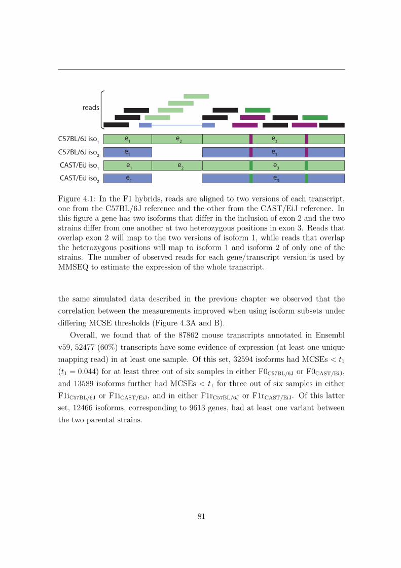
C57BL/6J iso1
C57BL/6J iso2e1
e1 e2 e3
e3
CAST/EiJ iso1
CAST/EiJ iso2
e1 e2 e3
e3e1
reads
Figure 4.1: In the F1 hybrids, reads are aligned to two versions of each transcript,one from the C57BL/6J reference and the other from the CAST/EiJ reference. Inthis figure a gene has two isoforms that differ in the inclusion of exon 2 and the twostrains differ from one another at two heterozygous positions in exon 3. Reads thatoverlap exon 2 will map to the two versions of isoform 1, while reads that overlapthe heterozygous positions will map to isoform 1 and isoform 2 of only one of thestrains. The number of observed reads for each gene/transcript version is used byMMSEQ to estimate the expression of the whole transcript.
the same simulated data described in the previous chapter we observed that the
correlation between the measurements improved when using isoform subsets under
differing MCSE thresholds (Figure 4.3A and B).
Overall, we found that of the 87862 mouse transcripts annotated in Ensembl
v59, 52477 (60%) transcripts have some evidence of expression (at least one unique
mapping read) in at least one sample. Of this set, 32594 isoforms had MCSEs < t1
(t1 = 0.044) for at least three out of six samples in either F0C57BL/6J or F0CAST/EiJ,
and 13589 isoforms further had MCSEs < t1 for three out of six samples in either
F1iC57BL/6J or F1iCAST/EiJ, and in either F1rC57BL/6J or F1rCAST/EiJ. Of this latter
set, 12466 isoforms, corresponding to 9613 genes, had at least one variant between
the two parental strains.
81

Figure 4.2: The expression levels of all transcripts in one of the F0 libraries areplotted against the respective Monte Carlo standard errors. The MCSEs are relatedto the expression level of the gene and to the number of reads uniquely mapping tothe transcript. The biggest drop in average MCSEs comes from the removal of geneswith no unique reads so a sensible threshold could be set to the highest MCSE ofthe set of genes which have at least one unique read (t1 = 0.044, horizontal dashedline).
82

log 2(F
0 CAST
/EiJ)
log2(F1CAST/EiJ)
log 2(F
0 C57B
L/6J
)
log2(F1C57BL/6J)
R = 0.90 R = 0.89
R = 0.96 R = 0.95
R = 0.97 R = 0.96
A
B
t1 = 0.044
t5 = 0.016
t0 = 0.381
0
5
10
15
0
5
10
15
0 5 10 15 0 5 10 15
Figure 4.3: To quantify our ability to estimate allele specific isoform expression wecreated an artificial F1 library as described in Section 3.2.1 and compared the origi-nal expression levels to the deconvoluted ones. (A) When comparing the expressionin the F0s to the allelic expression in the F1s without sub-setting by the MCSEswe found a very good agreement between the two (Pearson correlation >= 0.89).However, expression at the isoform level is less well estimated than at the gene level(see Figure 3.3, Pearson correlation >= 0.97). (B) When subsetting the set of iso-forms to only the ones under a MCSE threshold t (t ∈ {t1, t5} corresponding tothe maximum SE among isoforms with {1, 5} unique reads) the agreement improves(Pearson correlation >= 0.95).
83

4.2.1 Isoform level estimates reveal complex patterns of im-
printing
To identify isoforms with parent-of-origin effects we used the set of 12466 isoforms
that were reliably estimated in the F1s and that had a variant between the strains.
Using the same Beta-Binomial model and testing approach of the previous chapter
we found 422 and 434 autosomal transcripts paternally and maternally imprinted,
in total corresponding to 820 genes with at least one imprinted transcript at a false
discovery rate of 5% (Figure B.1). The number of genes found to be imprinted in
this analysis differs from the number found in the gene level analysis (535 imprinted
genes) partially because the set of features assessed in both analyses is not completely
overlapping due to different filtering procedures. To assess the comparability of the
imprinting calls found in both analyses, we looked at the 3231 genes with one and
only one annotated isoform assessed. We found that 98% of the genes imprinted at
the gene level were also imprinted at the transcript level, giving us confidence in our
imprinting calls. On the other hand, we have more power to detect imprinting at
the transcript level and found that 23% of the genes imprinted at the transcript level
were not imprinted at the gene level. This difference arises from two possible reasons:
1) because we used different data to generate the distribution of likelihood ratios for
the null hypothesis of no imprinting and 2) because the number of tests performed
at the isoform level analysis is larger. Finally, for multi-isoform genes the imprinting
calls between the gene level and the transcript level analysis can be different due to
complex imprinting patterns of the isoforms components. Comparing our imprinting
calls to the set of genes known to be imprinted in the mouse liver, we now identified
all 9 of them, including Airn, which was not detected as imprinted at the gene level
(Supp Table B.1).
Using the isoform level imprinting calls we observed 19 complex imprinting
events, including H13, in which isoforms from the same gene are imprinted in oppo-
site directions. For 17 of these genes, isoforms with opposite imprinting effects had
alternative first exons (AFE), alternative TSSs within the same promoter (ATSS)
or alternative polyAdenylation sites (APOL, Table 4.1), which is compatible with
current models of how complex imprinting is thought to happen. With the exception
of H13, none of these was previously described to be imprinted. We also looked for
84

Table 4.1: Genes with complex imprinting patterns. Transcripts are maternally (M)or paternally (P) expressed and differ due to alternative first exons (AFE), alter-native TSSs within the same promoter (ATSS), splicing (SPL) and/or alternativepolyAdenylation sites (APOL). Columns x and y contain the average log2 expressionfold change between the two alleles in the F1r and between the two alleles in theF1i, respectively.
gene transcript exp. event biotype y x1 5430407P10Rik-202 M ATSS, SPL, APOL protein coding 2.00 -0.471 5430407P10Rik-203 P ATSS, SPL, APOL protein coding -1.48 0.572 Ahctf1-001 M AFE, SPL, APOL protein coding 1.79 -1.012 Ahctf1-008 P AFE, SPL, APOL retained intron -1.67 2.363 Asl-006 M ATSS, SPL, APOL retained intron -0.06 -0.733 Asl-008 P ATSS, SPL, APOL protein coding -2.00 0.684 BC023814-206 M AFE, SPL, APOL protein coding 2.52 -2.834 BC023814-208 P AFE, SPL, APOL retained intron -2.67 0.625 Clpb-001 M ATSS, APOL protein coding 1.90 -0.825 Clpb-201 P ATSS, APOL protein coding -1.45 1.026 Cops5-001 M ATSS, SPL, APOL protein coding 0.24 -0.246 Cops5-003 P ATSS, SPL, APOL retained intron -1.76 0.487 Fgfr3-003 M AFE, SPL, APOL retained intron 2.79 -0.857 Fgfr3-201 P AFE, SPL, APOL protein coding -0.68 0.488 H13-001 M AFE, ATSS, SPL, APOL protein coding 3.15 -2.758 H13-002 M AFE, ATSS, SPL, APOL protein coding 2.81 -6.388 H13-004 M AFE, ATSS, SPL, APOL retained intron 2.98 -1.038 H13-005 P AFE, ATSS, SPL, APOL retained intron -3.21 4.078 H13-006 P AFE, ATSS, SPL, APOL protein coding -3.00 5.468 H13-201 M AFE, ATSS, SPL, APOL protein coding 2.37 -5.658 H13-202 M AFE, ATSS, SPL, APOL protein coding 2.39 -1.809 Khdrbs1-001 P SPL, APOL NMD -1.38 4.599 Khdrbs1-002 M SPL, APOL protein coding 4.10 -2.2810 Khk-002 P ATSS, SPL, APOL protein coding -1.97 1.9410 Khk-003 M ATSS, SPL, APOL protein coding 4.07 -2.6711 Nelf-014 M not overlap proc. transcript 2.57 -0.4811 Nelf-016 P not overlap proc. transcript -1.18 4.3812 Orai1-001 M SPL, APOL protein coding 2.16 -2.0012 Orai1-201 P SPL, APOL protein coding -5.51 2.8813 Rbpms-202 M SPL, APOL protein coding 4.54 -2.0113 Rbpms-203 P SPL, APOL protein coding -1.58 0.4814 Recql5-001 M AFE, SPL protein coding 2.17 -1.8914 Recql5-002 P AFE, SPL proc. transcript -2.85 1.4314 Recql5-005 M AFE, SPL proc. transcript 2.61 -0.8015 Sat2-001 M ATSS, SPL, APOL protein coding 4.04 -2.5615 Sat2-003 P ATSS, SPL, APOL retained intron -3.99 0.8916 Sfrs11-001 P ATSS, SPL, APOL protein coding -3.53 2.8416 Sfrs11-008 M ATSS, SPL, APOL NMD 0.72 -3.7717 Tmub1-001 M AFE, APOL protein coding 2.65 -1.5817 Tmub1-002 P AFE, APOL protein coding -1.46 1.2018 Usp4-201 P SPL protein coding -4.01 3.5718 Usp4-202 M SPL protein coding 5.10 -2.7919 Zcchc6-201 M SPL protein coding 0.45 -0.4419 Zcchc6-202 P SPL protein coding -0.19 0.16
85

Table 4.2: Clusters of genes imprinted in opposite directions. Transcripts are ma-ternally (M) or paternally (P) expressed. Columns x and y contain the average log2
expression fold change between the two alleles in the F1r and between the two allelesin the F1i, respectively.
cluster transcript strand expressed biotype y x1 Arrdc3-001 + M protein coding 0.89 -1.161 RP23-128L22.2-001 - P processed transcript -1.74 1.252 AC087541.3-201 + M lincRNA 0.70 -2.902 Rsl1d1-001 - P protein coding -1.21 7.763 Airn-001 + P antisense -1.87 2.613 Airn-201 + P antisense -1.36 3.683 Igf2r-001 - M protein coding 7.67 -8.103 Mas1-001 - M protein coding 3.28 -2.923 RP23-432O2.2-001 + P processed pseudogene -1.51 2.724 Aip-002 - P protein coding -2.47 0.514 Tmem134-005 + M protein coding 3.07 -4.285 H13-001 + M protein coding 3.15 -2.755 H13-002 + M protein coding 2.81 -6.385 H13-004 + M retained intron 2.98 -1.035 H13-005 + P retained intron -3.21 4.075 H13-006 + P protein coding -3.00 5.465 H13-201 + M protein coding 2.37 -5.655 H13-202 + M protein coding 2.39 -1.805 Mcts2-001 + P protein coding -6.95 7.366 Pex10-001 + P protein coding -1.09 0.966 Rer1-001 - M protein coding 3.13 -3.347 Mrps25-003 - P processed transcript -1.35 3.277 Nr2c2-001 + M protein coding 1.17 -1.478 1300018I17Rik-207 - M retained intron 1.25 -0.868 Zfp276-001 + P protein coding -5.49 0.95
86

clusters of overlapping genes with at least two genes imprinted in different direc-
tions. We detected 8 clusters, including the well known H13-Mcts2 and Igf2r-Airn
examples (Table 4.2). Interestingly, six of the clusters included at least one protein
coding and one anti-sense non-coding transcript. Gene silencing by an anti-sense
non coding gene has been observed for a number of known imprinted genes (Igf2r,
Kcnq1 and Gnas, [72]) and these results suggest that our novel clusters may be
regulated in a similar way. Given that DNA methylation is thought to be involved
in most genomic imprinting events we looked for known allele specific differentially
methylated regions (DMRs) occurring within or nearby our complex genes and clus-
ters. In the absence of a more appropriate dataset, we compared our imprinting calls
to the set of 55 DMRs found in mouse brain by Xie et al. [165] and did not find
support for any of our novel complex imprinted genes and gene clusters. However,
we think these genes are strong candidates for true liver imprinted genes and a vali-
dation of these imprinting calls by targeted bisulphite sequencing and allele-specific
PCR is planned.
4.2.2 Approximately 8% of genes have differential isoform
usage between C57BL/6J and CAST/EiJ
To allow a complete characterisation of differential isoform usage between C57BL/6J
and CAST/EiJ, we restricted the analysis to the set of genes with two and only two
expressed isoforms. Of this set we considered the 2073 genes for which: 1) at
least one of the isoforms is well estimated (SE < 0.044) in at least three out of
six samples in F0C57BL/6J and in F0CAST/EiJ and 2) the gene expression estimate in
at least one of the 12 F0 mice is >= 10. To find genes where there is differential
isoform usage between the parental strains independently of whether the gene is
differentially expressed we compared the proportions of expression of one of the
isoforms over the total gene expression.
For this classification we used a model based on the Beta-Binomial distribution.
For each gene with two isoforms, where isoform 1 is chosen randomly, we introduce
the following notation:
xi = expression of isoform 1 in the ith C57BL/6J F0 mouse
87

nxi = total gene expression in the ith C57BL/6J F0 mouse
yi =expression of isoform 1 in the ith CAST/EiJ F0 mouse
nyi = total gene expression in the ith CAST/EiJ F0 mouse
Here i takes values between 1 and 6 (F0 samples). We make the following dis-
tributional assumptions:
xi ∼ Bin(nxi , pxi ) and yi ∼ Bin(nyi , p
yi )
And we impose the following prior distributions upon px and py:
pxi ∼ Be(αx, βx) and pyi ∼ Be(αy, βy)
We can then model the null hypothesis of no differential isoform usage by restrict-
ing the hyperparameters α and β such that the prior distributions are the same
(αx = αy and βx = βy). In the alternative hypothesis of differential isoform usage
the F0C57BL/6J and F0CAST/EiJ data may come from two different distributions (αx,
αy, βx, βy are independent parameters). To choose between the two hypotheses, the
maximum likelihood of each model was calculated and the likelihood ratio between
them was obtained. The two models are nested so we performed a likelihood ratio
test by comparing the likelihood ratio to the quantiles of a chi-squared distribution
with two degrees of freedom.
At a false discovery rate cut-off of 10% and requiring a change of at least 5% in
isoform ratio, we found 161 (8%) genes with differential isoform usage between the
strains (Figure 4.4A). Genes with differential isoform usage were enriched for the
“ABC transporters” and “complement and coagulation cascades” KEGG pathways
at a FDR of 22% (Table 4.3). In particular, ABC transporters play an important role
in lipid trafficking and are involved in the regulation of cholesterol metabolism [167].
Of the three ABC transporters and two additional genes thought to be involved in
cholesterol regulation and which we identified as having differential isoform usage,
four had isoforms that coded for different annotated proteins (Abca8b, Abcc10,
Hpn and Apob). Whether the protein isoforms are functionally different needs to
88

be further investigated. However, differential usage of these protein coding isoforms
could be implicated in previously reported differences between cholesterol levels in
the C57BL/6J and CAST/EiJ strains [1].
Figure 4.4: Differential isoform usage between strains. (A) A normalised distance(t-statistic) between the proportion of the major isoform in the C57BL/6 strain andthe proportion of the same isoform in CAST/EiJ is plotted against the significancelevel of the difference. Genes with differential isoform usage are coloured red. (B)The proportion of randomly chosen isoform 1 over total gene expression (isoform 1+ isoform 2) is plotted for each strain. For a few genes the major isoform switchesby more than 50%.
Differences in isoform usage were continuously distributed amongst the set of
161 genes. For 26% of these genes the isoform usage switched from one isoform to
the other between strains (Figure 4.4B). The set of genes for which isoform usage
changed by more than 50% is significantly enriched for targets of the following
microRNAs in the UTR regions exclusive to only one of the isoforms in each gene:
miR-92a (Arhgef17 and Ibtk) and miR-711 (Slc25a35 and 1700001C19Rik, Table
4.3). Although intriguing, this requires further investigation.
89

Table 4.3: GO enrichments for genes with differential isoform usage (obtained withGeneTrail [7]).
KEGG pathway expected observed FDR (BH) enrichmentComplement and coagula-tion cascades
1.01 5 0.0405 up
ABC transporters 0.92 3 0.2151 upmiRNA expected observed FDR (BH) enrichmentmmu-miR-711 0.03 2 0.0006 upmmu-miR-92a 0.09 2 0.0034 up
4.2.3 Most isoform regulatory divergence is caused by reg-
ulatory variants in trans
To examine the regulatory divergence of isoform usage we used the set of autosomal
genes with two isoforms expressed in both the F0s and the F1s that: 1) were not
imprinted in either the gene level or the isoform level analysis, 2) had heterozygous
loci in both isoforms, 3) had an expression level >= 10 in at least one sample in the
F0s and 4) had an expression level >= 5 in at least one of the F1s. For each gene
we used an extension of the statistical framework described in the previous section
to classify it by its pattern of regulatory divergence in cis, in trans or in cis+trans.
Genes for which there is a differential usage of isoforms between the parents are
classified as either cis or trans regulated if the ratio of allele specific proportion is
the same as the ratio of the proportions in the parents, or if the proportions are
equal between the alleles, respectively (Figure 4.5). Genes with divergent isoform
usage that do not fit the above are classified as regulated by variants both in cis
and in trans. Briefly, for each gene with two isoforms, where isoform 1 is chosen
randomly and (xi, nxi ) and (yi, n
yi ) are as defined in the previous section, we intro-
duce the following notation for the F1s:
zj = expression of isoform 1 from the C57BL/6J allele of the jth F1 mouse
nzj = total gene expression of the C57BL/6J allele of the jth F1 mouse
wj =expression of isoform 1 from the CAST/EiJ allele of the jth F1 mouse
nwj = total gene expression of the CAST/EiJ allele of the jth F1 mouse
90

Subsequently, we make similar distributional assumptions as for the F0s:
zj ∼ Bin(nzj , pzj) and wj ∼ Bin(nwi , p
wj )
pzj ∼ Be(αz, βz) and pwj ∼ Be(αw, βw)
To assign genes to each category we determined a p-value for alternative isoform
usage between the parental strains and another p-value for alternative isoform us-
age between the alleles in the F1s with a chi-squared test as for the F0 data alone.
Genes were classified as conserved if both p-values were greater or equal to 0.01, as
cis if both were less than 0.01 and as trans if the p-value for differential isoform
usage between the parental strains was less than 0.01 and the p-value for differential
isoform usage between the alleles in the F1s was greater than 0.1. Genes that did
not fall into any of the above categories were classified as cis+trans. Furthermore,
we required a minimum change of 5% in the isoform ratio to classify genes as having
divergent isoform usage.
Without thresholding by standard error (i.e. potentially including genes in which
both isoforms are poorly estimated) we were able to classify 2662 genes. Of this set,
the majority (2202, 93%) show evidence of being regulated in a conserved fashion.
In stark contrast with the regulation of gene expression levels, for genes in which
isoform usage has diverged between the strains, the largest class comprises genes
that are regulated by variants purely in trans (98, 4%). The second largest class
corresponds to genes regulated by a combination of variants in cis and variants in
trans (51, 2%), while genes that are regulated by variants purely in cis amounts
to only 19 (<1%). When applying the classification to subsets of genes in which
at least one isoform is well estimated we observe that the frequency of genes in
each regulatory class is robust to changing cut-offs on the standard errors (Figure
4.6). When we examined the set of genes classified as being regulated in trans
among the set of 1249 genes with at least one isoform with SE < t1 we observed a
significant enrichment at a FDR of 10% of the following gene ontology categories:
ABC transporters, cardiomyopathy and regulation of actin cytoskeleton. For both
the set of genes regulated in trans and the set of genes regulated by variants both
in cis and in trans we observed an enrichment for targets of a number of miRNAs
91

cis trans
6x
F0
6x
F0
12x
F1
C57BL/6J
CAST/EiJ
70%
70%
70%
70%
40%
70%
40%
40%
40%
40% 60%
60%
Figure 4.5: Example of a cis and trans effect for a gene with two isoforms. In thecis example isoform 1 accounts for 70% of gene expression in F0C57BL/6J, while inF0CAST/EiJ it accounts for 40% of the expression due to a variant in a regulatoryregion in cis to the gene, for example a variant in a splice site. In the F1 theisoform proportions of the parents are reproduced in the different alleles. In thetrans example the change in isoform usage is due to a diffusible element, for exampledue to a changed splicing factor. In the F1 the isoform proportions may be similaror different to the parental proportions but are equal between the alleles.
92

(Tables 4.4 and 4.5), while the set of genes regulated in cis and the set of conserved
genes were not significantly enriched for any pathways or trans acting factors.
Table 4.4: Gene set enrichment analysis for genes regulated in trans (obtained withGeneTrail [7]).
KEGG pathway expected observed FDR (BH) genesABC transporters 0.35 2 0.0943 Abca8b Abcc10ARVC cardiomyopathy 0.35 2 0.0943 Itgb1 Atp2a2Dilated cardiomyopathy 0.42 2 0.0943 Itgb1 Atp2a2HCM cardiomyopathy 0.42 2 0.0943 Itgb1 Atp2a2Regulation of actin cy-toskeleton
1.46 4 0.0943 Pip4k2b Itgb1Cyfip1 Ssh2
miRNA expected observed FDR (BH) enrichmenthsa-miR-525-3p 0.94 5 0.0473 Hpn Ascc2 Peci
Trfr2 Spred2mmu-miR-674 0.31 3 0.0473 Peci Ssh2 Sfxn4mmu-miR-92a 0.88 5 0.0473 Rogdi Ddb1
Arhgef17 IbtkSsh2
mmu-miR-339-5p 0.69 4 0.0516 Rogdi Cd74Sipa1l3 Zdhhc5
mmu-miR-340-3p 0.12 2 0.0516 Trfr2 Zfp691
4.3 Discussion
To investigate the divergence of isoform usage in mammals we tested the relative
contribution of regulatory variants acting only in cis, only in trans and both in
cis and in trans between mouse subspecies using an F1 hybrid system. For this
we relied on allele specific isoform level expression estimates, which we obtained by
aligning RNA-sequencing reads to annotated cDNA sequences and using a prob-
abilistic model to deconvolve expression levels. Exploiting data and annotation
simultaneously improves the power of our analysis, however, previously unobserved
genes or isoforms will be missed. One way to address this in the future is to comple-
ment our analysis by adding isoform sequences predicted by a transcript discovery
93

Table 4.5: Gene set enrichment analysis for genes regulated both in cis and in trans(obtained with GeneTrail [7]).
miRNA expected observed FDR (BH) enrichmentmmu-miR-744 0.28 3 0.0409 Agtpbp1 Sema4g
Sh3bgrl3hsa-miR-560 0.17 2 0.0706 Abtb1 Tmcc1hsa-miR-602 0.14 2 0.0706 Trip10 Vkorc1l1hsa-miR-525-5p 0.31 2 0.0752 Gramd3 Sec24chsa-miR-603 0.28 2 0.0752 Gsn Abtb1mmu-miR-296-3p 0.37 2 0.0752 Abtb1 Vkorc1l1mmu-miR-30a 0.73 3 0.0752 Gramd3 Tmcc1
Vkorc1l1mmu-miR-30b 0.84 3 0.0752 Gramd3 Tmcc1
Vkorc1l1mmu-miR-30c 0.82 3 0.0752 Gramd3 Tmcc1
Vkorc1l1mmu-miR-30e 0.73 3 0.0752 Gramd3 Tmcc1
Vkorc1l1mmu-miR-324-5p 0.28 2 0.0752 Abtb1 Tmcc1mmu-miR-466f-5p 0.68 3 0.0752 Gstt3 Sema4g Gsnmmu-miR-467e 0.34 2 0.0752 Tmcc1
1110002N22Rikmmu-miR-467d 0.42 2 0.0908 Agtpbp1 Tmcc1
94

1 2 3 4 5 6
1458 1342 1249 1177 1110 1047
t0 t1 t2 t3 t4 t5 t6 t7 t8 t9 t10
0.0
0.2
0.4
0.6
0.8
1.01629 1249 1188 1145 1116 1077 1058 1035 1020 1010 998
prop
of g
enes
in e
ach
regu
lato
ry c
lass
by varying SE threshold t by varying number of samples s
A B
Figure 4.6: Classification of genes according to their pattern of isoform expressiondivergence. Genes for which isoform usage has not diverged between the two strainsare classified as conserved (coloured black), while genes in which isoform usage hasdiverged are classified as cis (coloured yellow), trans (coloured red) or cis and trans(coloured purple). We used different subsets of genes to verify that the proportionsallocated to each class are robust to changing the threshold on the standard errors.(A) Proportion of genes in the different classes for each subset of n genes (alongthe x-axis on top) with at least one isoform with SE below each threshold t (t ∈{t0, t1, ..., t10} corresponding to the maximum SE amongst isoforms with {0, 1, ..., 10}unique reads, respectively; along the x-axis bottom) in at least three out of sixsamples in F0C57BL/6J and in F0CAST/EiJ, and in at least six out of 12 samples inF1C57BL/6J and in F1CAST/EiJ. (B) Proportion of genes in the different classes foreach subset of n genes (along the x-axis on top) with at least one isoform with SEbelow threshold t1 = 0.044 in at least s out of six samples in F0C57BL/6J and inF0CAST/EiJ, and in at least 2s out of 12 samples in F1C57BL/6J and in F1CAST/EiJ
(along the x-axis bottom).
95

method to the reference transcript FASTA file and using it in the alignment and
mapping steps of the MMSEQ workflow.
Because parent-of-origin effects are a confounding factor in our analysis we used
initial and reciprocal crosses to identify and remove from the analysis imprinted
genes. Within our imprinted set we identified a small number of novel loci (24)
subject to complex imprinting patterns in which isoforms of the same gene and/or
overlapping genes show opposite parent-of-origin effects. This set, if validated by
an independent method, would significantly expand the number of loci previously
known to have such patterns. We are currently planning this validation using allele-
specific pyrosequencing and qRT-PCR experiments.
Our analysis of differences in isoform usage between the two strains using the F0s
revealed that 8% of genes with two expressed isoforms had divergent isoform usage.
This number is broadly consistent with a recent RNA-seq study which found that
6.5% to 28% of testis-expressed genes had alternative splice differences between at
least one pair of Mus musculus subspecies [56], and with a study which found that 7%
of genes expressed in liver undergo differential alternative splicing or have different
transcription start or end sites between humans and chimpanzees [13]. The number
of genes with differential isoform usage is smaller than the number of genes found
to have differential gene expression, however its magnitude suggests that differences
in isoform usage contribute to transcriptome divergence between mouse subspecies.
Using the full hybrid system we characterised the regulatory divergence for genes
with two and only two expressed isoforms. We consider that this simplification is
not likely to bias our results, however, our analysis method could be extended in
the future to include all multi-isoform genes by using a Dirichlet-Multinomial model
instead of the Beta-Binomial. Within the set of genes for which isoform usage has
diverged between the strains we found that the majority was regulated by variants
in trans, a large proportion was regulated by variants both in cis and trans, and a
small proportion of genes was regulated only is cis. The proportions allocated to
each regulatory class were very different from those found for the regulation of gene
expression levels and suggest that the mechanisms regulating overall gene expression
levels and isoform usage are under different evolutionary constraints.
One important challenge in understanding the regulation of splicing is that al-
ternative isoform usage results from multiple, potentially independent, regulatory
96

pathways. First, alternative isoforms may arise from alternative transcription start
sites (TSSs) within the same or between different promoters. The latter is most
likely achieved by differences in the regulation of the recruitment of the transcrip-
tional machinery to each promoter. The regulatory mechanism of the former is not
well understood but given that TSS selection occurs downstream of the recruitment
of the transcriptional machinery, it is likely that it differs from the mechanism of
selection between promoters [66]. Secondly, alternative isoform usage can arise from
alternative splicing, which is in part regulated by a mechanism involving trans acting
splicing factors binding to cis regulatory loci within the gene region. This mecha-
nism is again likely to be different from the mechanisms regulating other alternative
isoform producing events. Finally, alternative isoforms also arise from alternative
polyadenylation site usage. The regulation of the choice of polyadenylation site is
still not well understood, but it is thought to involve cis-acting sequences in the
pre-mRNA and trans acting members of the polyadenylation processing machin-
ery and RNA binding proteins. Given that different alternative splicing generating
events are regulated by different mechanisms, each event might involve different
proportions of cis and trans acting regulatory elements. The results presented in
this chapter combined different mechanisms of differential isoform regulation which
is potentially mis-leading.
To explore this further, we examined the proportion of genes in each regulatory
class for the subset of genes with two and only two isoforms. When looking at
our set of genes we found that the majority (54%) had at least one annotated
alternative splicing event, a large proportion had an alternative first exon (40%),
about a third had an alternative last exon and another third had an alternative TSS
within the same promoter. However, most genes had a combination of event types
(Figure 4.7) and separating genes by an exclusive event type reduced our sets to the
order of low hundreds and less, which we deemed too small to reliably characterise
regulation. Despite this limitation, one way in which the predominance of trans
acting regulators in isoform usage regulation could be explained is by the extensive
occurrence of alternative splicing events. The regulation of alternative splicing is
thought to be significantly driven by cis-acting regulatory regions located in the
gene’s exons or introns. These sequences are under considerable more constraint
than many of the cis-regulatory regions located in intergenic regions that control
97

overall gene expression levels. Hence, variants that act in trans might be a more
likely explanation for divergent isoform usage.
In summary, our study provides the first unbiased characterisation of the regu-
lation of alternative isoform usage in a mammalian system. It demonstrates that a
small but significant number of genes have alternative isoform usage between two
closely related mouse strains and that among this set, the majority are regulated
by variants that have arisen in trans. This result contrasts with the high preva-
lence of regulation both in cis and in trans and exclusively in cis of gene expression
levels. One likely explanation for this is that the cis-regulatory regions controlling
alternative isoform production are under stronger sequence constraint. However,
the pleiotropic arguments for the preferential accumulation of cis regulatory vari-
ants over time presented in the previous chapter may also be pertinent in this case
and we do not exclude the possibility that the proportion of cis acting variants will
increase with species divergence time. An informative extension of this work would
be to characterise gene and isoform divergence between strains that have diverged
at different times, which would allow a better understanding of the processes that
underlie speciation.
98

alternative first exon
alternative TSSwithin same exon splicing
alternativelast exon
104
7 234
83
0
50
376
75
174
79
0
0114
332
0
Figure 4.7: Number of genes with two and only two expressed isoforms by type ofalternative isoform producing event.
99

Chapter 5
Concluding remarks
High-throughput sequencing of RNA (RNA-Seq) allows for the first time the simul-
taneous measurement of sequence and expression of RNAs and the analysis of these
data requires novel bioinformatics approaches. In my work I have developed meth-
ods for the analysis of RNA-seq data and made contributions to the understanding of
regulation of gene expression and splicing. First, I implemented a complete pipeline
for data quality assessment, pre-processing and expression estimation of RNA-seq
datasets. This pipeline was, sometimes with modifications, applied to most of my
subsequent work. Second, I investigated the genome-wide evolution of gene expres-
sion in mammals by estimating the relative contribution of regulatory variants in
cis or in trans to the divergence of gene expression in a mouse model. Instrumental
for this work was the reliable estimation of allele-specific expression levels. For this,
I have used an existing method for estimating gene and isoform level expression
from RNA-seq data called MMSEQ and developed a methodology for applying it
to the estimation of allele-specific expression. Using the estimates thus obtained,
I observed that a large fraction of genes has divergent expression between the two
mouse strains. Of these, a very small minority could be explained by variants acting
purely in trans, while a big proportion was attributable to variants acting in cis. The
majority of genes, however, were regulated by multiple regulatory variants acting in
cis and in trans with opposing effects on gene expression. I propose that the most
likely explanation for this is the widespread occurrence of compensatory mutations
in gene expression evolution. Finally, I used the same experimental system and
methodology to study the evolution of isoform regulation. For this, I assessed the
relative contribution of regulatory variants in cis or in trans to the divergence of
100

isoform usage between the mouse strains. I found that isoform usage has diverged
to a lesser extent than overall expression levels. The largest fraction of genes was
regulated by variants acting in trans, a big proportion was attributable to multiple
variants in cis and in trans and only a small minority of genes was regulated by
variants purely in cis. These results suggest that the mechanisms regulating overall
gene expression levels and isoform usage are under different evolutionary constraints.
The development of new technology is providing an increasingly detailed charac-
terisation of the cell’s transcriptome. In the last two chapters I have demonstrated
how RNA-seq enables the elucidation of evolutionary mechanisms by providing the
sensitivity necessary to measure allele-specific expression. Although RNA-seq is
currently the most unbiased method for genome-wide measurement of gene expres-
sion, library preparation protocols still introduce considerable technical biases and
expression is routinely obtained over many, possibly heterogeneous, cells. More-
over, the requirements to fragment the RNA or cDNA molecules and the ability to
sequence only short reads precludes accurate identification of the full sequence of
each transcript present in a sample. These are still limiting factors in our ability
to progress from expression studies focused on overall expression levels averaged
over many cells to studies focused on individual transcripts in single cells. Looking
further into the future, the development of full length single molecule sequencing
in a single cell promises to surpass many of these limitations, providing a more
fine-grained understanding of the mechanisms governing gene expression.
101

Appendix A
Supplementary material for
Chapter 3
A.1 Experimental methods
The text in this experimental methods section is based on material provided by Ms.
Sarah Leigh-Brown, who conducted all the experimental work. The text in A.1.1
and A.1.2 is based on material included in Sarah’s Ph.D thesis submitted to the
University of Cambridge in September 2011.
A.1.1 Animal housing and handling
All mice used in this study were housed and handled in accordance with the Animals
(Scientific Procedures) Act 1986. Mice were housed and cared for in the Cambridge
Research Institute Biological Resource Unit with a twelve hour light/dark cycle,
and were provided with chow food from Lab Diet plus water ad libitum. Mice were
sacrificed by cervical dislocation at 4-6 months of age, between the hours of 9:30am
and 11:30am. The liver was then cut and the mouse perfused with PBS by injection
into the heart. Subsequently, the liver was removed and the gall bladder and hepatic
vein cut away. A sample of approximately 50mg-100mg was taken from a single liver
102

lobe and frozen on liquid nitrogen for storage at -80C until use.
A.1.2 Sequencing library preparation
For each liver sample, total RNA was extracted using the RNeasy Mini kit (Qiagen
74104) as per manufacturers instructions. RNA was checked for buffer contamina-
tion and approximate concentration on the Nanodrop spectrophotometer (Thermo
scientific). Before further processing, each total RNA sample was treated to digest
contaminating DNA. From each sample, polyadenylated mRNA was enriched from
the total RNA using the PolyATract mRNA isolation system. Directional double-
stranded cDNA was generated using the Superscript Double-Stranded cDNA Syn-
thesis kit (Invitrogen), with Uracil substituted for Thymine in the second strand.
250ng of double-stranded cDNA was fragmented prior to library preparation by
sonication in the Diagenode Bioruptor set on Hi for 5 minutes of 30 seconds on/off
cycles, repeated twice; each sonicated cDNA sample was then treated to generate
blunt ended double-stranded DNA. Following end repair, libraries were treated to
add an overhanging Adenine nucleotide and Illumina paired-end (PE) adapters were
ligated on both ends of each clone in the library. Strand-specificity was introduced
by digesting the second strand of cDNA using a uracil-specific enzyme. Each library
was subsequently amplified using PCR with Illuminas PE primers. Size selection
was performed by gel electrophoresis and 200-300 base pair fragments were extracted
from a 2% agarose gel. Finally, the quality of each library was tested prior to se-
quencing using the Agilent Bioanalyzer (Agilent). Libraries were sequenced on an
Illumina GAIIx in the genomics core facility of the Cambridge Research Institute.
A.1.3 Pyrosequencing
Genes were randomly selected for validation, following exclusion of genes that showed
evidence of imprinting and those that showed highly variable expression levels be-
tween biological replicates. Single nucleotide variants (SNVs) were identified using
the UCSC genome browser, and forward, reverse, and sequencing primers were de-
signed to target each SNV using PyroMark Assay Design software from Qiagen.
Each set of primers was tested for specificity in silico using Blat and in the labo-
103

ratory using quantitative PCR and using pyrosequencing on BL6xCAST genomic
DNA.
Pyrosequencing was performed on the Pyromark Q96 MD system, using the al-
lele specific quantification program. First, total RNA was isolated from the liver
of one initial F1 cross and one reciprocal F1 cross mouse, and double stranded
cDNA was generated using the Superscript II double-stranded cDNA kit (Invitro-
gen). Three technical replicate PCR reactions were performed on each cDNA sample
using one biotinylated and one non-biotinylated primer. PCR products were puri-
fied and enriched using streptavidin sepharose beads on the Pyromark vacuum prep
workstation. Pyrosequencing was performed on the enriched PCR products using
Pyromark Gold Q96 reagents and Pyromark MD software (Qiagen). The Pyromark
software determined an allelic ratio for each of three technical replicates, and the
average was determined from all six replicates of each genomic locus.
104

A.2 Supplementary Figures
Figure A.1: Samples cluster by strain. Plot of the first two principal componentsfor all 24 samples. Each F1 sample is represented once for each allele. All of thesix C57BL/6J F0 samples cluster together (coloured black) and with the C57BL/6Jallele of the 12 F1 samples (grey). All of the CAST/EiJ samples (brown) clustertogether with the CAST/EiJ allele of the 12 F1 samples (light brown).
105

% BL6 allele
80
R² = 0.9895
0
20
40
60
80
100
0 20 40 80 100
RN
Ase
q f
ollo
wed
by
MM
Seq
Pyrosequencing60
Figure A.2: Allelic Ratio measured by RNAseq and Pyrosequencing. Validationof allele-specific measurements made using RNA-seq. On the y-axis, a measure ofallele specific expression (using the C57BL6/J allele as reference) determined fromRNA-seq is plotted for five genes. On the x-axis, the corresponding measure ofallele-specific expression determined from pyrosequencing is shown. For three outof five genes, pyrosequencing was performed at two SNPs.
106
Figure A.3: Distribution of likelihood ratios for the test of imprinting. The dis-tribution of likelihood ratios obtained from the real data is plotted in the top twopanels, and the null distribution of likelihood ratios for the null hypothesis of noimprinting is plotted in the bottom two panels. In both cases the right hand plotshows a zoomed in version of the plot on the left.
107

−15 −10 −5 0
0.00
Den
sity
0.05
0.10
0.15
0.20
0.25
0.30
log10 expression estimate standard errors
Figure A.4: Density of the standard errors of the gene allelic expression estimatesobtained with MMSEQ in the F1s for each class (conserved - black, cis - yellow,trans - red, CIS+trans - blue, cis+TRANS - green, cis-TRANS - orange, CIS-transbrown). The standard errors are closely related to the number of unique readsmapping to each allele-gene and reflect the number of variants and the coverageover these.
108

Figure A.5: No relationship between conservation score and standard error esti-mates. The standard errors of the allelic expression estimates obtained with MM-SEQ in the F1s are plotted against the exonic conservation rates. There is norelationship between the two.
109

Figure A.6: Promoter sequence conservation rates for the different classes of regu-latory divergence.
110

Figure A.7: The relative GERP scores of the different classes (conserved - black, cis- yellow, trans - red, imprinted - white, cis and trans - purple) are robust to changesin the threshold used to call a nucleotide as conserved.
111

2 4 6 8 10 12
−6
−4
−2
0
2
4
log2 expression C57BL/6J allele + CAST/EiJ allele
log 2 C
57BL
/6J
alle
le /
CAS
T/Ei
J al
lele
Figure A.8: Imprinting continuum. The log2 total expression across both alleles(x-axis) is plotted against the log2 fold change between the alleles (y-axis) for allimprinted genes in one of the F1i samples.
112

A.3 Supplementary Tables
A.3.1 Supplementary Table A.1
Table A.1: Table of samples used in the study with the number of
raw and correctly aligned reads.
sampleID Strain numberReads numberAligned
do876 C57BL/6J 30373020 16187363
do877 C57BL/6J 32907241 21150758
do878 C57BL/6J 32075256 20178289
do879 C57BL/6J 30192493 18658862
do922 C57BL/6J 33152941 19497103
do923 C57BL/6J 29979442 16681710
do883 CAST/EiJ 33511533 11729077
do884 CAST/EiJ 32950724 13764947
do920 CAST/EiJ 29951804 15804537
do924 CAST/EiJ 27222930 14309559
do925 CAST/EiJ 29485779 14417501
do926 CAST/EiJ 25918629 11282255
do931 CAST/EiJ 19732873 9876140
reciprocal cross
do880 CAST/EiJxC57BL/6J 33063510 11630078
do882 CAST/EiJxC57BL/6J 33454400 11002668
do919 CAST/EiJxC57BL/6J 31814198 11001313
do927 CAST/EiJxC57BL/6J 27973105 16389873
do928 CAST/EiJxC57BL/6J 29362228 16697260
do929 CAST/EiJxC57BL/6J 19967614 10732085
do930 CAST/EiJxC57BL/6J 24502787 12087333
initial cross
113
do881 C57BL/6JxCAST/EiJ 32221296 10407915
do921 C57BL/6JxCAST/EiJ 32712218 14352188
do1087 C57BL/6JxCAST/EiJ 28333765 20518957
do1134 C57BL/6JxCAST/EiJ 44587843 19529138
do1135 C57BL/6JxCAST/EiJ 12353269 3428026
do1156 C57BL/6JxCAST/EiJ 12137349 3408161
114
A.3.2 Supplementary Table A.2
Table A.2: Overlap of the top 10% more highly variable genes in
C57BL/6J and CAST/EiJ
geneID geneName
ENSMUSG00000070394 1810027O10Rik
ENSMUSG00000029725 2010007H12Rik
ENSMUSG00000030587 2200002D01Rik
ENSMUSG00000062619 2310039H08Rik
ENSMUSG00000032712 2810474O19Rik
ENSMUSG00000060657 4921513D23Rik
ENSMUSG00000050459 4930470H14Rik
ENSMUSG00000048489 8430408G22Rik
ENSMUSG00000048249 A930001N09Rik
ENSMUSG00000029482 Aacs
ENSMUSG00000047370 AC046145.1
ENSMUSG00000025936 AC101743.1
ENSMUSG00000058064 AC102377.2
ENSMUSG00000083396 AC107815.5
ENSMUSG00000078081 AC109220.1
ENSMUSG00000067736 AC116997.1
ENSMUSG00000081094 AC121131.3
ENSMUSG00000069367 AC121903.1
ENSMUSG00000045886 AC121926.1
ENSMUSG00000061833 AC122242.2
ENSMUSG00000080893 AC122339.3
ENSMUSG00000089238 AC123039.1
ENSMUSG00000085995 AC124977.2
ENSMUSG00000058603 AC129545.2
115

geneID geneName
ENSMUSG00000074565 AC131780.1
ENSMUSG00000074564 AC131780.11
ENSMUSG00000074562 AC131780.2
ENSMUSG00000074561 AC131780.4
ENSMUSG00000087580 AC131780.5
ENSMUSG00000079719 AC131780.7
ENSMUSG00000074566 AC131780.8
ENSMUSG00000040323 AC133589.1
ENSMUSG00000088844 AC138229.1
ENSMUSG00000089895 AC138320.1
ENSMUSG00000067038 AC139040.1
ENSMUSG00000057036 AC139675.1
ENSMUSG00000083626 AC141643.2
ENSMUSG00000087778 AC147020.1
ENSMUSG00000073640 AC149589.2
ENSMUSG00000078300 AC150660.1
ENSMUSG00000043346 AC151288.1
ENSMUSG00000069196 AC154266.1
ENSMUSG00000079936 AC155937.1
ENSMUSG00000079360 AC158396.3
ENSMUSG00000022473 AC158787.2
ENSMUSG00000067547 AC158901.1
ENSMUSG00000084416 AC158958.3
ENSMUSG00000078103 AC161518.1
ENSMUSG00000074880 AC166937.1
ENSMUSG00000079329 AC174479.1
ENSMUSG00000021867 AC174479.4
ENSMUSG00000072676 AC175032.1
ENSMUSG00000060317 Acnat2
116

geneID geneName
ENSMUSG00000021228 Acot3
ENSMUSG00000062825 Actg1
ENSMUSG00000020473 Aebp1
ENSMUSG00000069833 Ahnak
ENSMUSG00000019256 Ahr
ENSMUSG00000089876 AL603707.1
ENSMUSG00000079971 AL611985.1
ENSMUSG00000078250 AL669969.1
ENSMUSG00000090229 AL672231.1
ENSMUSG00000089691 AL732309.1
ENSMUSG00000074846 AL732330.1
ENSMUSG00000090094 AL805896.1
ENSMUSG00000060628 AL833805.2
ENSMUSG00000075014 AL837506.1
ENSMUSG00000075015 AL837506.2
ENSMUSG00000089526 AL928940.1
ENSMUSG00000089784 AL929562.1
ENSMUSG00000032786 Alas1
ENSMUSG00000035561 Aldh1b1
ENSMUSG00000013076 Amotl1
ENSMUSG00000072115 Ang
ENSMUSG00000002289 Angptl4
ENSMUSG00000034647 Ankrd12
ENSMUSG00000054702 Ap1s3
ENSMUSG00000032080 Apoa4
ENSMUSG00000040564 Apoc1
ENSMUSG00000074336 Apoc4
ENSMUSG00000035133 Arhgap5
ENSMUSG00000019947 Arid5b
117

geneID geneName
ENSMUSG00000055116 Arntl
ENSMUSG00000074794 Arrdc3
ENSMUSG00000038539 Atf5
ENSMUSG00000034218 Atm
ENSMUSG00000031441 Atp11a
ENSMUSG00000003072 Atp5d
ENSMUSG00000016252 Atp5e
ENSMUSG00000050856 Atp5k
ENSMUSG00000038717 Atp5l
ENSMUSG00000028238 Atp6v0d2
ENSMUSG00000021738 Atxn7
ENSMUSG00000029787 Avl9
ENSMUSG00000018821 Avpi1
ENSMUSG00000041935 AW549877
ENSMUSG00000034780 B3galt1
ENSMUSG00000040225 Bat2l2
ENSMUSG00000026987 Baz2b
ENSMUSG00000002083 Bbc3
ENSMUSG00000053175 Bcl3
ENSMUSG00000022508 Bcl6
ENSMUSG00000030256 Bhlhe41
ENSMUSG00000067336 Bmpr2
ENSMUSG00000015943 Bola1
ENSMUSG00000047721 Bola2
ENSMUSG00000040481 Bptf
ENSMUSG00000090245 BX571735.1
ENSMUSG00000042460 C1galt1
ENSMUSG00000036887 C1qa
ENSMUSG00000015451 C4a
118

geneID geneName
ENSMUSG00000029385 Ccng2
ENSMUSG00000002944 Cd36
ENSMUSG00000024610 Cd74
ENSMUSG00000028755 Cda
ENSMUSG00000023067 Cdkn1a
ENSMUSG00000056501 Cebpb
ENSMUSG00000061825 Ces2
ENSMUSG00000049422 Chchd10
ENSMUSG00000024843 Chka
ENSMUSG00000027577 Chrna4
ENSMUSG00000032578 Cish
ENSMUSG00000008153 Clstn3
ENSMUSG00000001506 Col1a1
ENSMUSG00000025981 Coq10b
ENSMUSG00000041729 Coro2b
ENSMUSG00000036751 Cox6b1
ENSMUSG00000031231 Cox7b
ENSMUSG00000020300 Cpeb4
ENSMUSG00000090134 CR974462.1
ENSMUSG00000023272 Creld2
ENSMUSG00000062382 CT009486.1
ENSMUSG00000045999 CT010467.3
ENSMUSG00000003555 Cyp17a1
ENSMUSG00000063415 Cyp26b1
ENSMUSG00000005547 Cyp2a5
ENSMUSG00000040660 Cyp2b9
ENSMUSG00000042248 Cyp2c37
ENSMUSG00000032808 Cyp2c38
ENSMUSG00000056035 Cyp3a11
119

geneID geneName
ENSMUSG00000066072 Cyp4a10
ENSMUSG00000028715 Cyp4a14
ENSMUSG00000028240 Cyp7a1
ENSMUSG00000072680 D14Ertd449e
ENSMUSG00000055296 D730040F13Rik
ENSMUSG00000059824 Dbp
ENSMUSG00000001666 Ddt
ENSMUSG00000035967 Ddx26b
ENSMUSG00000069045 Ddx3y
ENSMUSG00000044748 Defb1
ENSMUSG00000030313 Dennd5b
ENSMUSG00000082691 Dynlt1-ps1
ENSMUSG00000046179 E2f8
ENSMUSG00000038418 Egr1
ENSMUSG00000042302 Ehbp1
ENSMUSG00000090264 Eif4ebp3
ENSMUSG00000038754 Elovl3
ENSMUSG00000041220 Elovl6
ENSMUSG00000028445 Enho
ENSMUSG00000040857 Erf
ENSMUSG00000061286 Exosc5
ENSMUSG00000006920 Ezh1
ENSMUSG00000042595 Fam199x
ENSMUSG00000025153 Fasn
ENSMUSG00000042423 Fbrs
ENSMUSG00000022788 Fgd4
ENSMUSG00000031594 Fgl1
ENSMUSG00000024222 Fkbp5
ENSMUSG00000061175 Fnip2
120

geneID geneName
ENSMUSG00000040891 Foxa3
ENSMUSG00000038415 Foxq1
ENSMUSG00000070733 Fryl
ENSMUSG00000050708 Ftl1
ENSMUSG00000021453 Gadd45g
ENSMUSG00000028671 Gale
ENSMUSG00000052957 Gas1
ENSMUSG00000031821 Gins2
ENSMUSG00000029638 Glcci1
ENSMUSG00000078162 Gm10481
ENSMUSG00000078965 Gm10481
ENSMUSG00000074106 Gm10627
ENSMUSG00000038550 Gm129
ENSMUSG00000047822 Gm6484
ENSMUSG00000078903 Gm6710
ENSMUSG00000045472 Gm9798
ENSMUSG00000046721 Gm9811
ENSMUSG00000034837 Gnat1
ENSMUSG00000024978 Gpam
ENSMUSG00000045441 Gprin3
ENSMUSG00000031450 Grk1
ENSMUSG00000060803 Gstp1
ENSMUSG00000038155 Gstp2
ENSMUSG00000050440 Hamp
ENSMUSG00000056978 Hamp2
ENSMUSG00000069919 Hba-a1
ENSMUSG00000069917 Hba-a2
ENSMUSG00000073940 Hbb-b1
ENSMUSG00000052305 Hbb-b2
121

geneID geneName
ENSMUSG00000038664 Herc1
ENSMUSG00000007836 Hnrnpa0
ENSMUSG00000031722 Hp
ENSMUSG00000007872 Id3
ENSMUSG00000020429 Igfbp1
ENSMUSG00000039323 Igfbp2
ENSMUSG00000026185 Igfbp5
ENSMUSG00000066232 Ipo7
ENSMUSG00000032293 Ireb2
ENSMUSG00000038894 Irs2
ENSMUSG00000052837 Junb
ENSMUSG00000071076 Jund
ENSMUSG00000006740 Kif5b
ENSMUSG00000062901 Klhl24
ENSMUSG00000023043 Krt18
ENSMUSG00000035202 Lars2
ENSMUSG00000039704 Lmbrd2
ENSMUSG00000036957 Lrfn3
ENSMUSG00000037095 Lrg1
ENSMUSG00000001870 Ltbp1
ENSMUSG00000028670 Lypla2
ENSMUSG00000033902 Mapkbp1
ENSMUSG00000025409 Mbd6
ENSMUSG00000032418 Me1
ENSMUSG00000021268 Meg3
ENSMUSG00000059149 Mfsd4
ENSMUSG00000033943 Mga
ENSMUSG00000008035 Mid1ip1
ENSMUSG00000035621 Midn
122

geneID geneName
ENSMUSG00000027820 Mme
ENSMUSG00000088272 mmu-mir-2133-2
ENSMUSG00000087974 mmu-mir-2143-3
ENSMUSG00000076258 mmu-mir-689-2
ENSMUSG00000020000 Moxd1
ENSMUSG00000010406 Mrpl52
ENSMUSG00000063011 Msln
ENSMUSG00000031765 Mt1
ENSMUSG00000029009 Mthfr
ENSMUSG00000089873 Mup13
ENSMUSG00000073830 Mup14
ENSMUSG00000073832 Mup15
ENSMUSG00000078675 Mup16
ENSMUSG00000078673 Mup19
ENSMUSG00000041333 Mup4
ENSMUSG00000058523 Mup5
ENSMUSG00000078687 Mup8
ENSMUSG00000022346 Myc
ENSMUSG00000020900 Myh10
ENSMUSG00000034427 Myo15b
ENSMUSG00000025402 Nab2
ENSMUSG00000029478 Ncor2
ENSMUSG00000002379 Ndufa11
ENSMUSG00000022820 Ndufb4
ENSMUSG00000020716 Nf1
ENSMUSG00000056749 Nfil3
ENSMUSG00000001911 Nfix
ENSMUSG00000042419 Nfkbil1
ENSMUSG00000031773 Nlrc5
123

geneID geneName
ENSMUSG00000026077 Npas2
ENSMUSG00000037583 Nr0b2
ENSMUSG00000005893 Nr2c2
ENSMUSG00000002393 Nr2f6
ENSMUSG00000023034 Nr4a1
ENSMUSG00000055254 Ntrk2
ENSMUSG00000043013 Onecut1
ENSMUSG00000045991 Onecut2
ENSMUSG00000020189 Osbpl8
ENSMUSG00000064225 Paqr9
ENSMUSG00000038967 Pdk2
ENSMUSG00000020893 Per1
ENSMUSG00000028957 Per3
ENSMUSG00000026773 Pfkfb3
ENSMUSG00000020205 Phlda1
ENSMUSG00000030660 Pik3c2a
ENSMUSG00000043760 Pkhd1
ENSMUSG00000087141 Plcxd2
ENSMUSG00000002831 Plin4
ENSMUSG00000028680 Plk3
ENSMUSG00000017754 Pltp
ENSMUSG00000041653 Pnpla3
ENSMUSG00000039771 Polr2j
ENSMUSG00000038489 Polr2l
ENSMUSG00000022383 Ppara
ENSMUSG00000000440 Pparg
ENSMUSG00000046794 Ppp1r3b
ENSMUSG00000067279 Ppp1r3c
ENSMUSG00000027346 Prei4
124

geneID geneName
ENSMUSG00000010175 Prox1
ENSMUSG00000020415 Pttg1
ENSMUSG00000020594 Pum2
ENSMUSG00000047824 Pygo2
ENSMUSG00000049404 Rarres1
ENSMUSG00000040423 Rc3h1
ENSMUSG00000054031 Rdh18
ENSMUSG00000035504 Reep6
ENSMUSG00000036120 Rfxank
ENSMUSG00000026475 Rgs16
ENSMUSG00000059810 Rgs3
ENSMUSG00000002233 Rhoc
ENSMUSG00000050310 Rictor
ENSMUSG00000033107 Rnf125
ENSMUSG00000089739 RP23-118A2.10
ENSMUSG00000081485 RP23-136K12.6
ENSMUSG00000082697 RP23-139C9.1
ENSMUSG00000078154 RP23-14F5.5
ENSMUSG00000066477 RP23-157H17.2
ENSMUSG00000048949 RP23-181M13.5
ENSMUSG00000042938 RP23-185F7.4
ENSMUSG00000075391 RP23-186B18.4
ENSMUSG00000043770 RP23-191F22.11
ENSMUSG00000087262 RP23-22L6.2
ENSMUSG00000087299 RP23-233B9.5
ENSMUSG00000081471 RP23-272G10.2
ENSMUSG00000081205 RP23-273C23.1
ENSMUSG00000090221 RP23-294G7.3
ENSMUSG00000085091 RP23-295E4.2
125
geneID geneName
ENSMUSG00000083594 RP23-298M2.10
ENSMUSG00000080888 RP23-330D3.2
ENSMUSG00000090136 RP23-356D13.4
ENSMUSG00000046840 RP23-36P22.4
ENSMUSG00000086231 RP23-386I18.2
ENSMUSG00000087306 RP23-396K15.2
ENSMUSG00000060989 RP23-425K3.1
ENSMUSG00000085001 RP23-438L23.2
ENSMUSG00000081448 RP23-451D4.10
ENSMUSG00000086922 RP23-459L15.3
ENSMUSG00000083696 RP23-465A17.2
ENSMUSG00000086320 RP23-99G21.3
ENSMUSG00000079224 RP24-114M8.2
ENSMUSG00000089940 RP24-163G22.1
ENSMUSG00000064193 RP24-364O14.1
ENSMUSG00000083087 RP24-371A24.1
ENSMUSG00000072940 RP24-417N21.2
ENSMUSG00000089855 RP24-69E21.3
ENSMUSG00000038900 Rpl12
ENSMUSG00000045128 Rpl18a
ENSMUSG00000058546 Rpl23a
ENSMUSG00000060938 Rpl26
ENSMUSG00000063316 Rpl27
ENSMUSG00000030432 Rpl28
ENSMUSG00000062997 Rpl35
ENSMUSG00000057863 Rpl36
ENSMUSG00000046330 Rpl37a
ENSMUSG00000007892 Rplp1
ENSMUSG00000025508 Rplp2
126

geneID geneName
ENSMUSG00000052146 Rps10
ENSMUSG00000061983 Rps12
ENSMUSG00000069972 Rps13
ENSMUSG00000037563 Rps16
ENSMUSG00000028234 Rps20
ENSMUSG00000025362 Rps26
ENSMUSG00000020460 Rps27a
ENSMUSG00000074115 Saa1
ENSMUSG00000057465 Saa2
ENSMUSG00000042978 Sbk1
ENSMUSG00000046229 Scand1
ENSMUSG00000022032 Scara5
ENSMUSG00000037071 Scd1
ENSMUSG00000029597 Sds
ENSMUSG00000029596 Sdsl
ENSMUSG00000041567 Serpina12
ENSMUSG00000031271 Serpina7
ENSMUSG00000044734 Serpinb1a
ENSMUSG00000020211 Sf3a2
ENSMUSG00000024042 Sik1
ENSMUSG00000019935 Slc17a8
ENSMUSG00000026819 Slc25a25
ENSMUSG00000022003 Slc25a30
ENSMUSG00000024131 Slc3a1
ENSMUSG00000081534 Slc48a1
ENSMUSG00000030237 Slco1a4
ENSMUSG00000017002 Slpi
ENSMUSG00000044349 Snhg11
ENSMUSG00000065637 SNORA14
127

geneID geneName
ENSMUSG00000084708 SNORA48
ENSMUSG00000084744 SNORA48
ENSMUSG00000064382 SNORA63
ENSMUSG00000089417 snoU90
ENSMUSG00000072941 Sod3
ENSMUSG00000022091 Sorbs3
ENSMUSG00000024427 Spry4
ENSMUSG00000020538 Srebf1
ENSMUSG00000006442 Srm
ENSMUSG00000021020 Srp54a
ENSMUSG00000071640 Stxbp3b
ENSMUSG00000000739 Sult5a1
ENSMUSG00000063450 Syne2
ENSMUSG00000053580 Tanc2
ENSMUSG00000020167 Tcf3
ENSMUSG00000022389 Tef
ENSMUSG00000020219 Timm13
ENSMUSG00000034917 Tjp3
ENSMUSG00000028132 Tmem56
ENSMUSG00000036676 Tmtc3
ENSMUSG00000022791 Tnk2
ENSMUSG00000033327 Tnxb
ENSMUSG00000028998 Tomm7
ENSMUSG00000048707 Tprn
ENSMUSG00000031431 Tsc22d3
ENSMUSG00000025511 Tspan4
ENSMUSG00000039438 Ttc36
ENSMUSG00000043091 Tuba1c
ENSMUSG00000026202 Tuba4a
128
geneID geneName
ENSMUSG00000058672 Tubb2a
ENSMUSG00000008348 Ubc
ENSMUSG00000033685 Ucp2
ENSMUSG00000042985 Upk3b
ENSMUSG00000026839 Upp2
ENSMUSG00000020163 Uqcr
ENSMUSG00000063882 Uqcrh
ENSMUSG00000071528 Usmg5
ENSMUSG00000032010 Usp2
ENSMUSG00000056342 Usp34
ENSMUSG00000065145 Vault
ENSMUSG00000037440 Vnn1
ENSMUSG00000037646 Vps13b
ENSMUSG00000035284 Vps13c
ENSMUSG00000017677 Wsb1
ENSMUSG00000057836 Xlr3a
ENSMUSG00000079845 Xlr4a
ENSMUSG00000064945 Y RNA
ENSMUSG00000047412 Zbtb44
ENSMUSG00000000552 Zfp385a
ENSMUSG00000047036 Zfp445
ENSMUSG00000073060 Zxda
129

A.3.3 Supplementary Table A.3
Table A.3: Table of genes with Parent-of-Origin effects. The aver-
age expression level of each gene for the C56BL/6J or CAST/EiJ
alleles (B or C) in the initial cross and reciprocal cross (F1i and
F1r) are given. Genes are either maternally expressed (M) or pa-
ternally expressed (P).
gene name chr F1iB F1iC F1rB F1rC expressed
0610011L14Rik 2 35.83 25.17 50.17 67 P
0910001L09Rik 5 447 518.17 582.17 498 M
1110004E09Rik 16 51.5 39.17 40.83 80.83 P
1110004F10Rik 7 153.67 106.17 117.67 157.83 P
1110007A13Rik 7 26.17 42.67 46.33 37.67 M
1110021J02Rik 17 22.17 7.83 13.17 20.83 P
1600014C10Rik 7 236.33 218 430.5 527 P
1700003E16Rik 6 3.67 1.67 5.17 9.5 P
2310021P13Rik 14 39.67 31.67 62.17 74.5 P
2510039O18Rik 4 52.67 66.5 129.33 105.83 M
2610036L11Rik 10 15.5 6 4.33 8 P
2810004N23Rik 8 93 63.5 74.17 88.5 P
2900092E17Rik 7 32.17 29.67 24.67 35.67 P
4933403F05Rik 18 45.33 50.17 61.83 56.5 M
4933439F18Rik 11 36.83 39.83 55 46.17 M
5430411K18Rik 18 11.67 14.5 22 18 M
5730419I09Rik 6 3.67 9.17 11.17 6.33 M
9130019O22Rik 7 4.33 2.17 3.33 5.5 P
A830010M20Rik 5 28.17 9 24 42.67 P
Aak1 6 3.83 1.17 5.67 6.5 P
Abcf3 16 100.5 85.17 107.67 133 P
130

gene name chr F1iB F1iC F1rB F1rC expressed
Abhd5 9 49 55.33 70 53.33 M
Abi2 1 1.5 3.83 3.17 2.17 M
Abr 11 2.17 4.67 5.5 2.67 M
AC079443.1 6 7.33 3.67 10.5 13 P
AC087780.9 1 2.17 1 1.67 3.5 P
AC087801.10 1 2 3.83 8.83 7.33 M
AC101915.1 1 0 3.17 5.33 1.17 M
AC102103.1 15 0 5.17 2.17 1 M
AC114905.1 1 9.33 7.83 14.67 18.83 P
AC115896.3 1 0 1.83 2.17 0 M
AC116677.2 3 6.5 7.67 10.33 2.83 M
AC120378.1 7 8.17 5.5 3 5.5 P
AC133646.1 18 1.67 5.83 6.83 2 M
AC135240.1 5 68.17 87 124.33 109.17 M
AC135567.1 16 9.5 6.17 7.83 16.67 P
AC137950.1 15 5 3.33 4.17 6.83 P
AC152395.1 15 2.5 0.67 2.67 5.5 P
AC152453.1 10 6.17 0.83 2 5 P
AC163646.1 14 9.17 0.17 16.5 0.17 M
AC165252.1 16 5.67 1.67 6.83 13.17 P
AC165327.2 19 1.5 3.83 6.17 3 M
Actr10 12 123.67 103.33 90.83 105.67 P
Acvr1 2 15.67 19.83 34.67 26.5 M
Agps 2 10.17 4.33 6.17 10.17 P
Akap5 12 7 0.83 2.5 2.83 P
Aktip 8 42.67 27 33 36.67 P
AL607072.1 11 20.5 15.33 8.67 16.17 P
AL772271.1 2 2.17 4.83 10.17 4.17 M
AL805896.1 4 0.5 19.67 4.17 0 M
131

gene name chr F1iB F1iC F1rB F1rC expressed
Alg8 7 31 25.17 21.67 27 P
Alkbh6 7 54.33 36.67 55.5 65.33 P
Ambra1 2 31.83 38.17 58.5 35.33 M
Ampd2 3 125.83 103.83 186.83 205.83 P
Ankrd40 11 113.67 139.17 135.67 113.67 M
Ankrd49 9 14.33 5.83 7.33 11 P
Aoc2 11 4.83 3 1.17 9.67 P
Ap1s3 1 0.17 6 8.33 3.67 M
Ap3s1 18 162.67 69 72.33 92.33 P
Ap3s2 7 25.67 22.83 28.17 34.67 P
Arhgap26 18 111.83 57.5 102 135.5 P
Arhgef10 8 2 3.33 7.5 3.33 M
Arhgef7 8 30.67 32.83 49 37 M
Arid5b 10 5 14 20.83 18.83 M
Atg16l1 1 30.83 45 80.83 61.33 M
Atp6v1h 1 97.17 129.33 128.33 86.5 M
Atrnl1 19 11.67 19.17 23.33 19.5 M
Aup1 6 571.5 642.17 780 692 M
B230319C09Rik 6 1.5 4 2 1.5 M
Bak1 17 87.5 75 42.83 46.5 P
BC024139 15 25.5 22.83 28.17 35.33 P
BC024479 9 12.67 6 6.33 11.83 P
BC050254 5 0 17.33 35.17 49.5 M
Bcl7c 7 193.83 51.17 77.67 121.83 P
Becn1 11 154.33 141.33 227.33 260.17 P
Brp44l 17 1222.67 1218 1021.33 1127.83 P
C130022K22Rik 6 12.67 16.5 18.67 13.17 M
C2cd2l 9 76.67 79.67 139.5 114.17 M
Cables2 2 48.67 46.17 70.83 84 P
132

gene name chr F1iB F1iC F1rB F1rC expressed
Calcrl 2 6.83 4 4.17 7.5 P
Caml 13 45.5 74 65.17 54.67 M
Cant1 11 44.33 52.17 88 72.5 M
Card6 15 17.67 11.33 15.67 20.33 P
Casp9 4 42.67 32.5 42.67 50.67 P
Cbfa2t2 2 7.67 9.67 15 10.17 M
Cbx6 15 2.33 8.33 8 5.17 M
Ccdc107 4 316 266.5 269.5 286.83 P
Ccdc141 2 15.83 15.83 12.83 21.17 P
Ccdc97 7 48.33 55.67 96 88.33 M
Ccnd2 6 3.33 0 0.83 4 P
Ccnd3 17 121.33 73.17 95.17 143.33 P
Cct6a 5 146.33 129 160.67 182.67 P
Cd151 7 160.33 144.17 186.83 218.5 P
Cd300lg 11 24.83 27.33 28.5 23.67 M
Cd320 17 16.83 5.33 18.33 22.67 P
Cd52 4 15.17 43.33 10 3 M
Cd84 1 1 6.83 2 2.17 M
Cdc123 2 119.33 151.5 145.83 124.17 M
Cdc16 8 62.83 50.83 56.33 66.5 P
Cdc37l1 19 35 38.5 40.33 32 M
Cdca4 12 4.67 7.83 9.17 6 M
Cdk20 13 11.67 13.83 23.5 14.17 M
Cdkn1c 7 2.33 2.33 10.33 0 M
Cenpa 5 11.5 12.83 19 10.5 M
Chmp5 4 141 179.67 138.83 126.67 M
Chmp7 14 83.5 65 104.83 131.67 P
Chpf 1 7.5 1.67 10.67 13.5 P
Chuk 19 237.67 205.83 225 238.33 P
133

gene name chr F1iB F1iC F1rB F1rC expressed
Cisd3 11 491.67 445.5 249.83 313.17 P
Clec1b 6 29.5 12.83 8.5 13.67 P
Cno 5 9.17 13 70.33 59.5 M
Cnot1 8 47.17 73.83 83.5 72 M
Cog8 8 67 81.17 102.83 77.67 M
Col13a1 10 3.83 6.17 9.5 5.5 M
Commd5 15 68.17 53.5 63.83 110 P
Cops5 1 145 160.33 198.5 165.33 M
Cops7a 6 258.5 235.67 334.67 428 P
Coq3 4 41.83 51.83 44 38 M
Cox10 11 35.67 25.67 32.5 36.5 P
Cpsf3 12 64 81.5 89.83 78.67 M
Crebl2 6 77.83 66.17 86.17 97.33 P
Crem 18 58.33 61.83 62.67 51.17 M
Crip1 12 54.67 0 0 24.17 P
Csnk1g3 18 31 36.83 33.33 26.67 M
Csnk2a2 8 32.17 39.33 30 46.83 P
CT025701.1 9 0.83 1.5 3 1.33 M
Ctbs 3 9.5 20.17 15 12.33 M
Ctdsp2 10 87.33 90.67 126.33 111.83 M
Cugbp1 2 69.67 114.67 117 98.33 M
Cugbp2 2 20 11.5 8.33 11.67 P
Cul3 1 48.83 59.33 88.5 46.33 M
Cul9 17 6.33 4.67 13.67 18 P
Cyb561d1 3 10.33 6.83 9.83 16 P
Cyb5r3 15 1874 227.17 555.67 1176.17 P
Cyp26b1 6 0 3.33 2.17 0 M
Cyp2c29 19 7483.83 7261 3326.67 3810.67 P
Cyp2c50 19 3645.33 3296.17 2155.33 2192.67 P
134

gene name chr F1iB F1iC F1rB F1rC expressed
Cyp2j9 4 26.83 29.17 32.83 19 M
D0H4S114 18 40.5 31 50.33 56.33 P
D10627 8 4.83 0.17 0.67 2.83 P
D930015E06Rik 3 20.67 23.17 40 28.83 M
Daam1 12 26.67 31 40.5 34 M
Dcaf10 4 14.67 31.67 29.67 24.67 M
Ddah2 17 6.83 1.33 10.17 18.5 P
Ddx24 12 71.5 63.83 70.83 86.33 P
Dennd2a 6 4.33 6.17 6.17 3.33 M
Dexi 16 97.83 105.67 178 138.83 M
Dgka 10 22 22.17 15.33 41.17 P
Dimt1 13 6.33 11 13.67 6.83 M
Dnaja2 8 215.83 238.33 237.83 203 M
Dnajc10 2 31.33 27.17 27.83 41.83 P
Dnhd1 7 4.33 20.83 20.33 11.67 M
Dolpp1 2 66.17 68.83 88.83 67.83 M
Dpp3 19 116.5 126.83 213 168 M
Dpp7 2 52.17 67.5 77 59.5 M
Dusp16 6 39.5 36 43.5 52.67 P
Dusp22 13 26.83 63.17 46.17 27.33 M
Dync1h1 12 37.17 33.17 61.17 68 P
Ebpl 14 667.67 628.17 609.83 735.5 P
Ecm1 3 509.67 538.33 535 454.33 M
Edc4 8 29.5 14.17 45.83 65.67 P
Eef1e1 13 37.67 49 29.17 47 P
Eefsec 6 75 56.17 111.67 121.17 P
Eif4e2 1 167.17 184.5 173 130.33 M
Entpd6 2 16.17 18.33 33.33 22.33 M
Epcam 17 6.33 1.5 1.83 5.5 P
135

gene name chr F1iB F1iC F1rB F1rC expressed
Erbb2ip 13 34.17 39.67 37.5 33.17 M
Eri2 7 7.17 9.83 8.67 5.5 M
Esam 9 24.83 25.17 28.5 18.5 M
Etaa1 11 6 3.33 4 5.83 P
Exoc3l 8 7.5 4.33 15.83 18.83 P
Exosc4 15 39.33 173.5 264.83 206.67 M
Fam103a1 7 97 139.67 89.33 81.83 M
Fam108c 7 158.83 181.17 245.67 210.5 M
Fam149b 14 37.33 45.67 60.17 52.67 M
Fam59a 18 12.5 8.83 16.67 24 P
Fam83f 15 2.5 4.17 8.5 6.17 M
Fancc 13 8.67 10.5 16.83 11.5 M
Farsb 1 103.83 82.67 78 109.5 P
Fbxl4 4 31 39.5 39.17 35.5 M
Fbxo28 1 10.67 6.67 10 12.17 P
Ficd 5 19.17 17.67 21.67 29.67 P
Foxp4 17 52.33 62.67 102.33 93.17 M
Frmd4a 2 3.67 4.17 8.67 4 M
Fyn 10 5.5 18.33 11.17 8.83 M
Glul 1 2668.17 2458.33 2465.5 2731.17 P
Gm10392 11 3.83 1 2.17 4.17 P
Gm10397 14 33.67 46.5 22 23.5 M
Gm9754 5 1.33 4 7.33 4.17 M
Gmppa 1 178 166 189.5 251.17 P
Gna13 11 26.5 23.83 32.33 43.33 P
Gnas 2 975.17 1361.67 1913.67 1541.67 M
Gnpat 8 85.17 93.33 125.5 106.83 M
Gnptg 17 77.5 58.83 65.83 81.5 P
Golga2 2 36.67 61.67 93 57 M
136

gene name chr F1iB F1iC F1rB F1rC expressed
Golph3l 3 2.83 16 7.83 4.33 M
Gpatch2 1 13.67 15.5 23 14.67 M
Gpn2 4 51.67 38 91 103 P
Grap 11 4.33 7.17 10.83 6.83 M
Grb10 11 0.83 5.83 7 3.33 M
Grpel1 5 145.83 257.5 201.5 178.17 M
H13 2 245.67 941.83 1036.17 284.5 M
Hamp2 7 5147.83 3628.83 1571.83 3802 P
Harbi1 2 28.33 38.5 40.5 30.5 M
Haus2 2 12.83 15.67 15.67 11.5 M
Haus8 8 10.5 10.83 12.67 6.17 M
Hbb-b2 7 1322.83 1424 485.5 453.17 M
Hcn3 3 42.33 46.67 72.67 154.17 P
Heatr2 5 23.33 19.67 24.67 36 P
Herc4 10 45.83 41.17 19.33 56.83 P
Hes1 16 45.33 40.33 31.17 54.5 P
Hmox2 16 141.17 58.17 103.5 136.17 P
Hsf2bp 17 7.5 1.5 7.17 6.67 P
Iars 13 38.5 42.67 60.17 47.17 M
Ict1 11 147.67 208.17 293.83 220.67 M
Iffo1 6 19.83 14.83 29.33 37.67 P
Ifi203 1 5.17 11.5 8.83 5.5 M
Ifit1 19 5.33 3.5 3.83 5.33 P
Igf2r 17 0.17 49.33 82.17 0.67 M
Impact 18 13.83 0.83 3 15.67 P
Ipp 4 23.83 14 21.5 25.33 P
Irs2 8 1.83 3.83 10.83 8.33 M
Itpkb 1 5.33 7.67 12.67 8.5 M
Jarid2 13 7.17 11.67 14.33 12.17 M
137

gene name chr F1iB F1iC F1rB F1rC expressed
Kcnc3 7 7.5 12.67 18.33 16.5 M
Kctd10 5 16.17 26.5 38 31.17 M
Kif1b 4 69.33 57 82.17 87.33 P
Klhl6 16 1.67 1.17 2.33 4.67 P
Kras 6 32.5 43.83 38.5 34.17 M
Krtcap3 5 13.5 4.83 13.5 20.83 P
l7Rn6 7 42 78.17 57.33 47.17 M
Laptm4a 12 584.17 2.17 290 250.33 P
Larp4b 13 22.17 29.33 35.83 29.83 M
Lats1 10 4.67 7.17 12.83 9.83 M
Lgals3 14 10 12 11 2.33 M
Lime1 2 5.67 20.67 44.83 18.17 M
Limk2 11 12.5 18.33 20.17 17.83 M
Lin7c 2 38.33 44.17 40.83 34.5 M
Lman2 13 515 458 668.17 904.83 P
Lmo4 3 50 44.83 39 66.83 P
Lrp3 7 49.83 40.67 91.5 106.17 P
Lrrc58 16 60.67 44.17 26.67 58.33 P
Lrwd1 5 16 18.83 32 20 M
Lsm3 6 69.17 24.5 14.33 26.17 P
Lsp1 7 13 4.17 3.33 7 P
Lst1 17 26.67 11.83 2.33 10.67 P
Maff 15 3.5 12.17 12.67 10.83 M
Map2k2 10 490.67 381.5 886.83 962.17 P
Map2k5 9 40 47.5 60.67 52.33 M
Map3k1 13 9.67 7.5 9.67 12.83 P
Map3k14 11 5.5 4.17 7.33 10.67 P
Map4k5 12 21 14.17 17.17 24 P
Mare 11 49.83 66 102.5 86.67 M
138

gene name chr F1iB F1iC F1rB F1rC expressed
Mars 10 124.17 183.17 232.83 198.33 M
Mas1 17 1.33 12.5 10.83 2.67 M
Masp1 16 177 204.83 223.5 206.17 M
Mbl1 14 580.5 575.83 603 639.33 P
Mcts2 2 47.17 0 0.67 38.17 P
Mdm4 1 5 9.67 14.17 9.17 M
Me1 9 542.17 551.33 545.83 463.67 M
Med28 5 102.83 74 78 86.83 P
Med31 11 11.17 4.17 2 9.33 P
Meg3 12 3.67 364.5 378.67 6.67 M
Mett11d1 14 32.5 42.33 49 33.5 M
Mettl2 11 18.17 17 22.33 32.33 P
Mfsd3 15 50.83 68.17 64.17 102.83 P
Mfsd4 1 16 22.5 45.67 28.67 M
Mgat2 12 20 70.33 52 29.33 M
Mmp23 4 14.5 3.33 2.5 4.83 P
Mogs 6 120 101.33 160.33 186.5 P
Mpdu1 11 387.5 296.67 374.67 399.83 P
Mpv17l2 8 151 57.67 122 161 P
Mrpl41 2 206 184 152.33 181 P
Mrps15 4 122 216.33 164.17 119.17 M
Msi2 11 19 24.67 24.83 20.83 M
Mt2 8 0 10.5 2.67 1.33 M
Myo1e 9 52.17 48.67 57.17 66.83 P
N6amt2 14 38.17 42.17 40.17 23.17 M
Naa15 3 28.83 19.83 18.83 26.5 P
Nadsyn1 7 95.83 93.67 95.33 125.17 P
Napg 18 29.83 26.33 24.33 32.67 P
Nat15 16 222.17 300.67 336.17 313.83 M
139

gene name chr F1iB F1iC F1rB F1rC expressed
Nat5 2 29.67 57.5 41.5 44 M
Ncald 15 15.17 19.17 24.33 14.33 M
Nceh1 3 33.33 15.67 27.17 34.17 P
Ndn 7 2.83 0 0 4.83 P
Ndufb6 4 682.33 818.5 654 547.83 M
Ndufs1 1 175.5 189.33 226.17 213.83 M
Neu1 17 105.5 87.5 137 184.5 P
Nfe2l1 11 190.5 167.17 195.67 244.5 P
Nip7 8 43.5 57.67 44.33 25.83 M
Nmnat1 4 51.5 45 53.17 64 P
Nmral1 16 38 19 20.17 38.33 P
Nr3c1 18 66.33 58.83 80.17 86.33 P
Nr4a1 15 0.33 2.83 4 0 M
Nsfl1c 2 247.17 169.33 221 318.5 P
Nt5c2 19 33.83 29 30.5 43 P
Nuak2 1 34.17 25.5 32.33 36.33 P
Nup153 13 15.17 11.17 16.17 18.67 P
Nupl1 14 14.5 3.33 8.67 13.83 P
Nxt1 2 40 40.67 32.17 47.5 P
Obfc2a 1 10.5 16 18.83 8.67 M
Oxa1l 14 169.5 174.17 266.17 216.5 M
P4ha2 11 24.5 14.83 21.5 25.83 P
Paip2 18 250.67 272.5 254.83 229.33 M
Pard6b 2 4.17 9 15.5 9.67 M
Pcgf6 19 22.33 16.83 16.83 24.33 P
Pcif1 2 66.33 72.67 147.17 59 M
Pcolce 5 40.33 29.83 38 42.83 P
Pcsk4 10 86.67 82.83 162.67 103.83 M
Pdcd2 17 59.33 100.17 105.17 41.83 M
140

gene name chr F1iB F1iC F1rB F1rC expressed
Pde4d 13 6.67 5.17 3 6.17 P
Peli2 14 11.5 14.5 20 11.83 M
Pgap3 11 6.33 3.33 7.67 9.83 P
Pgrmc2 3 140 143.33 200.17 165 M
Phactr4 4 37 45.17 46.67 41.33 M
Phc2 4 55.83 61.67 93 75.17 M
Phf1 17 48.17 54.67 71 64.83 M
Pigp 16 42.17 60.5 36.83 27.5 M
Pik3c3 18 23.33 29.33 34.67 29.67 M
Pik3cb 9 19.17 7.83 13.83 16.67 P
Pik3cd 4 5.67 0.83 3.83 5.33 P
Pisd-ps2 17 29.83 37.5 53.67 48.5 M
Pitpnm2 5 42.17 46.67 116.67 87.17 M
Pkdcc 17 39.17 46.67 112 72.5 M
Plekhg6 6 17.67 19.33 51.67 36 M
Pold4 19 134.33 91.17 83.33 99 P
Poldip2 11 277 296.67 337.5 304 M
Polm 11 10.83 15.83 21.67 19.83 M
Polr1b 2 17.33 34.67 43.67 35 M
Polr3g 13 10.5 11.33 22.33 4.83 M
Ppic 18 10.83 3.33 2.5 5.5 P
Ppm1a 12 111.5 106.83 103.33 230.17 P
Ppm1m 9 21.67 24.83 52.5 11.33 M
Ppp1r15a 7 22 30.17 41 27.5 M
Ppp3ca 3 29.67 34 36.17 24 M
Ppp4r2 6 21 47.33 39.83 26.5 M
Prdm11 2 3.67 7.5 9.17 4.5 M
Prepl 17 33.83 36.33 39.5 26.67 M
Prickle4 17 20.67 12.67 15.5 19.5 P
141
gene name chr F1iB F1iC F1rB F1rC expressed
Prkacb 3 39.67 53.5 55.17 42.33 M
Prmt2 10 0.67 4 4 3.17 M
Prpf40b 15 30.5 50 76 51.83 M
Psmb5 14 478.83 463 739.83 561.17 M
Psmd11 11 231.17 354.83 331.67 258.83 M
Psmd12 11 226.83 204.33 191.5 235.33 P
Ptbp2 3 4.17 17.33 13.67 10 M
Ptdss2 7 28.5 22.17 39.83 46.17 P
Ptpn18 1 5.83 2 2 4.67 P
Ptpn23 9 23 34 50.17 38.5 M
Ptprj 2 16.67 57.67 70 30.33 M
Pum1 4 45.33 37.5 48.67 59.67 P
Pvrl3 16 68 56.17 58.33 65 P
Rab11fip3 17 18 27 39.83 33.5 M
Rab2a 4 256 238.17 237.83 250.33 P
Rab33b 3 8.83 13.5 14.83 13 M
Rab4b 7 78.17 89.33 139.83 113.83 M
Rabac1 7 229 335 572.67 390.33 M
Rad23a 8 166.17 91.5 116.33 188.33 P
Ralgapa2 2 14.17 16 23.83 17.67 M
Raly 2 115.33 88.33 166 200.67 P
Ranbp1 16 183.17 122.67 115.83 158.67 P
Ranbp2 10 27.33 15.67 27 30.33 P
Rapgef2 3 15 9.83 16.67 22 P
Rarg 15 5.83 19.83 11 9.33 M
Rasgef1b 5 11.17 8.67 10.83 27.5 P
Rasl2-9 7 1.67 1 4.17 7.17 P
Raver1 9 39.83 55.5 87.83 65.17 M
Rbbp6 7 37.17 45.5 43.5 37.83 M
142

gene name chr F1iB F1iC F1rB F1rC expressed
Rbm15 3 11.17 3.67 13.33 17.33 P
Rbm19 5 11.67 11.5 28 16.33 M
Rbm4 19 32 12.67 32.83 38.5 P
Rbm47 5 90.5 70.67 124 153.83 P
Rbp1 9 68.83 63.33 29.67 61.33 P
Rbpms 8 66 105.5 96 91.5 M
Rcc2 4 49 45 83 95.17 P
Rcor3 1 8.17 0.5 3.67 6.67 P
Recql5 11 22.67 33.17 48.33 44 M
Rell1 5 19.17 12.83 20.33 29.83 P
Rer1 4 377.83 381.5 425.67 219.33 M
Rest 5 8 12 12.5 10.67 M
Rhbdf1 11 14 20.5 29.67 20 M
Rhob 12 28.67 20.33 143.17 175.67 P
Rnf126 10 64.5 116.17 210.67 167.83 M
Rnf168 16 15.5 4.5 7.5 11.67 P
Rnf34 5 13.17 21.5 20.67 17.5 M
Rnf5 17 348.33 404.67 496.33 394 M
Rnf7 9 146 36.67 117.67 183 P
Rom1 19 5.83 2.83 3.67 17.67 P
RP23-128L22.2 13 3.83 1 2 4.67 P
RP23-129P10.1 6 6.17 2.5 6 7.83 P
RP23-223C17.2 2 0.33 2.17 2.5 1.17 M
RP23-340E1.2 9 25.17 35.67 37 16 M
RP23-44L6.2 2 17.83 31.83 26 17.83 M
RP23-84C12.13 11 0.67 2 7.33 2.17 M
RP24-252K15.1 1 68.5 78 64.33 52 M
Rpl7a 2 1874.33 1637.17 1566.17 1723 P
Rpp40 13 24 13.5 18 20.83 P
143

gene name chr F1iB F1iC F1rB F1rC expressed
Rps14 18 266.17 405.67 536.83 372.5 M
Rps15a 7 555.5 787.33 438.83 335.33 M
Rps16 7 191.5 351.17 384.67 278.67 M
Rps6kb1 11 25 32 30.67 25.17 M
Rsad1 11 15.67 11.33 24.67 32.33 P
Rtn4rl1 11 21.67 15 18.83 22.33 P
Ruvbl2 7 30.67 35.67 59.83 49.33 M
S1pr1 3 131.17 120.5 145.33 156.17 P
Saa3 7 37 23.67 24.67 3.5 M
Samd8 14 27 23 24.17 30.33 P
Sat2 11 37 56.17 72 30.33 M
Scamp2 9 46.5 49.17 61.83 44.33 M
SCARNA13 12 26.83 1.83 4.17 6.33 P
Sccpdh 1 2.67 6.83 5.67 3 M
Sco1 11 34.5 28.67 25.33 32.83 P
Sdad1 5 11.67 9.5 11.5 14.17 P
Sec11a 7 248.83 138.67 117.33 175 P
Sec13 6 116.67 48 83.33 105.17 P
Sec23ip 7 30.17 27.5 28.5 35.5 P
Sec31a 5 315.67 378 397.67 384.17 M
Sec61b 4 739.5 700 781 464.17 M
Selp 1 4.67 9.17 9.83 7.5 M
Sema3f 9 4.33 7.67 11 9.83 M
Sepx1 17 2897.33 2670.33 2352.83 2664.33 P
Serpina9 12 3.67 0 0 4.17 P
Serpind1 16 1427 1454.83 1472.67 1353.5 M
Serpinh1 7 20.33 31.83 33.5 21.5 M
Sfrs13a 4 59.17 27.5 24.67 49.17 P
Sfxn3 19 3.5 2.5 3 5 P
144

gene name chr F1iB F1iC F1rB F1rC expressed
Sgce 6 17.67 0.83 1.17 13.17 P
Sgip1 4 5 2.17 0.67 5.17 P
Shfm1 6 568.83 620.83 582.17 512.83 M
Skp1a 11 619.67 996.17 625.67 573.67 M
Slc22a3 17 0.5 21 15.17 1 M
Slc25a36 9 3.83 0.83 1.33 3.67 P
Slc38a6 12 107.5 142 133.83 118.5 M
Slc39a14 14 189 203 297.33 263.5 M
Slu7 11 25.17 37 36.5 31.83 M
Smad7 18 19.17 17.17 29.83 39 P
Snf8 11 346.17 157.33 155.17 222.67 P
Snip1 4 15.5 33.67 31.17 26.5 M
SNORA26 12 19.17 0 1.33 5.33 P
SNORA32 9 0 3.33 3.33 0 M
SNORA74 14 3.33 15.17 9.17 15.17 M
Snrpb2 2 27.67 34.67 25.17 18.5 M
Snrpn 7 70.67 0 0.33 135.33 P
Snx4 16 46.5 47.17 63 48.67 M
Sp5 2 3.67 7.83 18 7 M
Spats2 15 6.5 7.17 14 8.17 M
Spcs2 7 146.33 186.67 160.5 115.33 M
Spef1 2 1.83 4.5 5 2.33 M
Spna2 2 69.17 95.83 149 127.5 M
Srpr 9 359.83 356.17 447.67 504 P
Ssbp1 6 119.5 108.67 71.5 91 P
Ssbp4 8 12.5 1.33 9.67 19.67 P
Stab1 14 64.33 82.83 94.5 76.17 M
Strap 6 132 123.17 151.33 175.33 P
Stt3a 9 193 201.17 204 182.83 M
145

gene name chr F1iB F1iC F1rB F1rC expressed
Stx6 1 9.5 13.33 29.67 26 M
Szt2 4 26.17 16.5 32.5 46.33 P
Tada1l 1 25.17 30.67 51.5 40.17 M
Taf4a 2 12.17 19 25.5 19.67 M
Tbc1d7 13 43.17 35.17 36.33 51.5 P
Tbx3 5 30.33 37.83 56.83 37.83 M
Tctex1d2 16 0.33 6.67 4.5 1.83 M
Tfpt 7 35.33 39.5 55.17 35.83 M
Tgs1 4 9.17 16.67 18.33 12.67 M
Thap3 4 40.83 27.17 49.67 71.83 P
Thap7 16 95.67 79.33 110.5 130.5 P
Thoc4 11 128.33 45.33 89.33 163.83 P
Tmco4 4 28.17 21.83 30.67 55.67 P
Tmem140 6 46.5 39.33 32.17 45 P
Tmem161b 13 11.5 17 14.67 9.5 M
Tmem184c 8 16.5 20.17 21.33 17.83 M
Tmem188 8 43.33 46.17 40.67 32.83 M
Tmem194 10 6.33 9.5 11.5 8.83 M
Tmem201 4 36.67 31.83 55.17 63.83 P
Tmem86a 7 19 28 27.5 25.5 M
Tnfaip1 11 45 53.17 53.5 45.83 M
Tnfrsf21 17 7.5 5.67 5.5 9.33 P
Tnpo3 6 38.83 52.83 54.5 43.5 M
Tnrc6a 7 33 13.5 26.67 32.33 P
Tox4 14 36 44.33 52.17 43.83 M
Trappc1 11 118.67 96.17 70.67 78.33 P
Trim13 14 14.17 10.67 7.17 10.83 P
Trim39 17 15.67 22.17 29.67 12.5 M
Trmt61a 12 5.83 10.83 25.83 15 M
146

gene name chr F1iB F1iC F1rB F1rC expressed
Trnt1 6 40.17 32.83 28.17 34.17 P
Trp53bp2 1 16.83 26 28.67 23 M
Trp53i11 2 20.83 16.67 16 19.83 M
Trp53inp2 2 333.33 321.5 330.5 353.83 P
Tsen34 7 82 97.83 188.17 101.67 M
Ttc14 3 21.33 15.17 14.33 21.33 P
Ttyh3 5 13.67 10.83 17.33 23.17 P
Twf2 9 8.33 4 5 13.67 P
Tyw1 5 36.17 30.83 58.83 68.5 P
U11 4 0 7.33 4.83 3.67 M
U2af1 17 237.67 401 345.33 198.5 M
Uba3 6 57.33 65 62.5 50 M
Uba7 9 5.17 10.83 17.5 8.17 M
Ube2e1 14 124.17 162.5 111.67 87 M
Ube2e3 2 78.33 36.33 49.33 64.33 P
Ube2g1 11 52.67 38.17 35.33 61.17 P
Ube2k 5 209.83 142.17 145.17 175.67 P
Ucp2 7 31.5 32.83 66.5 46.33 M
Ufsp1 5 11 10.67 11 22.5 P
Unc13b 4 5.83 7 16 9.17 M
Uqcrfs1 13 758 704.67 794 834 P
Usp14 18 60.17 107.5 76.33 67.5 M
Usp20 2 8.67 10.67 22.5 15.5 M
Usp36 11 24.17 19.33 42.17 46.5 P
Uvrag 7 33.33 26 39.83 49 P
Vamp4 1 16.67 23.5 28.33 20.83 M
Vim 2 40.5 58.17 56.83 39.33 M
Vps13c 9 6.67 7.83 15.67 10.83 M
Vwce 19 59.67 71.33 117.33 103 M
147

gene name chr F1iB F1iC F1rB F1rC expressed
Wasl 6 80.67 65.83 63.17 73.5 P
Wdr35 12 1.5 4 6.33 3.33 M
Wdr81 11 36.67 40.67 99.33 73.5 M
Wfdc2 2 14 19.17 24.83 18.67 M
Zbtb12 17 1 11.5 16.83 12.5 M
Zbtb16 9 11.67 16.5 7.33 5.33 M
Zbtb4 11 8.5 10.5 23.67 17.67 M
Zdhhc3 9 57 46.83 65.5 72.67 P
Zfhx2 14 3.5 7.83 10.83 8.33 M
Zfp113 5 5.5 9 7.33 5.33 M
Zfp13 17 0.17 3.33 3.33 2.5 M
Zfp143 7 7.17 14.83 11.5 9.17 M
Zfp235 7 1.67 4.17 8 5.83 M
Zfp509 5 4.67 7.17 15.33 9.5 M
Zfp69 4 3.5 2.17 3.17 6.33 P
Zfp706 15 247.17 221.33 237.17 313.83 P
Zfp760 17 5.67 3.67 3.17 4.83 P
Zfp846 9 3.5 4.33 6.33 2 M
Zkscan5 5 19.5 26.83 37.5 28.83 M
Znrf3 11 5.33 7.83 12.5 8.17 M
Zrsr1 11 29 1.67 2.5 26.83 P
148

A.3.4 Supplementary Table A.4
Table A.4: GO enrichments for genes regulated in cis (obtained
with GeneTrail [7]).
GO term expected observed FDR (BH) enrichment
nucleus 339.83 261 4E-05 down
gene expression 223.73 158 4E-05 down
cellular macromolecule metabolic process 345.34 269 4E-05 down
nucleic acid metabolic process 218.35 154 4E-05 down
RNA metabolic process 128.46 79 5E-05 down
transcription regulator activity 69.56 33 5E-05 down
transcription 146.46 96 8E-05 down
regulation of transcription, DNA-dependent 74.21 38 8E-05 down
regulation of nucleobase, nucleoside, nu-
cleotide and nucleic acid metabolic process
156.26 104 8E-05 down
RNA biosynthetic process 79.84 42 8E-05 down
nucleoplasm part 30.37 8 8E-05 down
regulation of nitrogen compound metabolic
process
157.48 105 8E-05 down
regulation of primary metabolic process 188.10 131 8E-05 down
transcription, DNA-dependent 79.35 42 8E-05 down
nuclear part 80.46 43 9E-05 down
regulation of transcription 140.83 92 1E-04 down
nucleic acid binding 178.06 124 0.0001 down
regulation of macromolecule biosynthetic pro-
cess
154.67 104 0.0001 down
regulation of macromolecule metabolic pro-
cess
179.53 126 0.0001 down
regulation of RNA metabolic process 75.803 41 0.0002 down
149

GO term expected observed FDR (BH) enrichment
regulation of biosynthetic process 160.67 111 0.0002 down
regulation of gene expression 159.32 110 0.0002 down
regulation of cellular biosynthetic process 159.08 110 0.0002 down
macromolecule metabolic process 377.18 309 0.0002 down
cellular macromolecule biosynthetic process 199.73 146 0.0003 down
nucleobase, nucleoside, nucleotide and nucleic
acid metabolic process
258.51 200 0.0004 down
macromolecule biosynthetic process 202.06 149 0.0004 down
nuclear lumen 47.88 22 0.0006 down
regulation of metabolic process 207.08 155 0.0006 down
transcription from RNA polymerase II pro-
moter
47.02 22 0.0009 down
nucleoplasm 35.02 14 0.0013 down
DNA binding 111.19 74 0.0016 down
organelle part 208.30 159 0.0016 down
intracellular 758.39 695 0.0017 down
regulation of cellular metabolic process 194.96 148 0.0022 down
regulation of transcription from RNA poly-
merase II promoter
43.72 21 0.0025 down
intracellular part 741.25 680 0.0031 down
primary metabolic process 473.31 412 0.0033 down
intracellular organelle part 204.14 158 0.0038 down
protein binding 369.71 313 0.0042 down
transcription factor complex 15.31 3 0.0044 down
positive regulation of metabolic process 58.29 33 0.0044 down
positive regulation of macromolecule
metabolic process
53.03 29 0.0044 down
organelle lumen 59.52 34 0.0044 down
sequence-specific DNA binding 28.29 11 0.0044 down
150
GO term expected observed FDR (BH) enrichment
intracellular organelle lumen 59.15 34 0.0050 down
membrane-bounded organelle 584.26 524 0.0050 down
intracellular membrane-bounded organelle 583.40 524 0.0061 down
transcription activator activity 19.96 6 0.0061 down
positive regulation of nucleobase, nucleoside,
nucleotide and nucleic acid metabolic process
40.29 20 0.0061 down
positive regulation of nitrogen compound
metabolic process
41.64 21 0.0061 down
macromolecular complex 180.51 139 0.0066 down
membrane-enclosed lumen 61.96 37 0.0071 down
transferase activity, transferring acyl groups 16.29 4 0.0074 down
RNA splicing 19.59 6 0.0074 down
cellular nitrogen compound metabolic process 277.49 229 0.0076 down
organelle 636.79 579 0.0076 down
positive regulation of gene expression 39.55 20 0.0084 down
positive regulation of macromolecule biosyn-
thetic process
42.13 22 0.0085 down
intracellular organelle 635.08 578 0.0085 down
cellular process 699.12 643 0.0087 down
transcription factor activity 37.84 19 0.0095 down
transferase activity, transferring acyl groups
other than amino-acyl groups
15.80 4 0.0095 down
positive regulation of biosynthetic process 44.33 24 0.0100 down
post-translational protein modification 86.33 58 0.0100 down
positive regulation of cellular metabolic pro-
cess
54.49 32 0.0103 down
acyltransferase activity 15.55 4 0.0110 down
negative regulation of RNA metabolic process 23.39 9 0.0113 down
151

GO term expected observed FDR (BH) enrichment
negative regulation of transcription, DNA-
dependent
23.27 9 0.0122 down
positive regulation of cellular biosynthetic pro-
cess
43.72 24 0.0130 down
nitrogen compound metabolic process 283.62 239 0.0190 down
positive regulation of transcription 37.72 20 0.0190 down
protein modification process 100.66 72 0.0194 down
cellular metabolic process 471.84 421 0.0215 down
regulation of biological process 351.58 305 0.0252 down
in utero embryonic development 22.04 9 0.0255 down
chordate embryonic development 30.37 15 0.0262 down
negative regulation of gene expression 32.70 17 0.0315 down
biological regulation 379.14 333 0.0326 down
negative regulation of nitrogen compound
metabolic process
31.23 16 0.0326 down
regulation of cellular process 330.89 287 0.0349 down
mRNA processing 25.59 12 0.0358 down
embryonic development ending in birth or egg
hatching
30.86 16 0.0386 down
chromatin organization 26.70 13 0.0409 down
chromosome organization 30.74 16 0.0409 down
negative regulation of nucleobase, nucleoside,
nucleotide and nucleic acid metabolic process
30.61 16 0.0430 down
negative regulation of transcription 28.90 15 0.0497 down
Metabolic pathways 97.76 133 0.0015 up
oxidoreductase activity 53.27 87 0.0002 up
cellular aromatic compound metabolic process 11.39 27 0.0009 up
oxidation reduction 51.80 82 0.0009 up
locomotory behavior 10.65 24 0.0046 up
152

GO term expected observed FDR (BH) enrichment
coenzyme binding 16.04 31 0.0084 up
cofactor binding 21.92 38 0.0153 up
carboxy-lyase activity 2.57 9 0.0157 up
mitochondrion 123.81 156 0.0277 up
T cell apoptosis 0.61 4 0.0315 up
FAD binding 6.37 15 0.0322 up
catalytic activity 379.50 426 0.0348 up
behavior 19.59 33 0.0455 up
electron carrier activity 7.96 17 0.0455 up
oxidoreductase activity, acting on CH-OH
group of donors
10.04 20 0.0466 up
cellular nitrogen compound biosynthetic pro-
cess
26.70 42 0.0468 up
allantoin metabolic process 0.37 3 0.0478 up
regulation of prostaglandin biosynthetic pro-
cess
0.37 3 0.0478 up
positive regulation of prostaglandin biosyn-
thetic process
0.37 3 0.0478 up
153
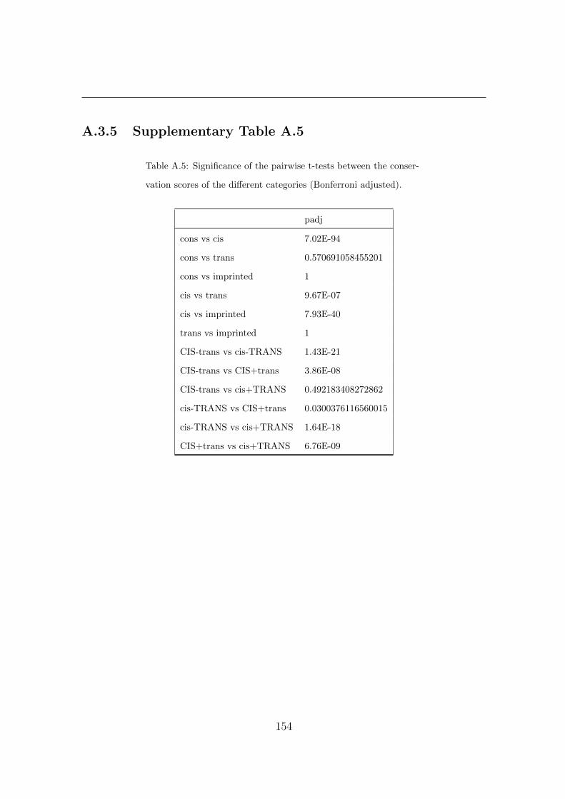
A.3.5 Supplementary Table A.5
Table A.5: Significance of the pairwise t-tests between the conser-
vation scores of the different categories (Bonferroni adjusted).
padj
cons vs cis 7.02E-94
cons vs trans 0.570691058455201
cons vs imprinted 1
cis vs trans 9.67E-07
cis vs imprinted 7.93E-40
trans vs imprinted 1
CIS-trans vs cis-TRANS 1.43E-21
CIS-trans vs CIS+trans 3.86E-08
CIS-trans vs cis+TRANS 0.492183408272862
cis-TRANS vs CIS+trans 0.0300376116560015
cis-TRANS vs cis+TRANS 1.64E-18
CIS+trans vs cis+TRANS 6.76E-09
154

Appendix B
Supplementary material for
Chapter 4
B.1 Supplementary Figures
155

●
●
●
●
●●
●●
●
●
●●
●
●
●
●
●
●
●
●
●
●
●
●
●
●
●●
●
●
●
●
●
●
●
●
● ●
●
●
●
●
●
●
●
●
●
●
●●
●
●
●
●●
●
●
●
●
●
●
●
●
●
●
●
●●
●
●
●
●
●
●
●
●●
●
●
●
●
●
●
●
●●
●●
●
●
●
●
●
●
●
●
●
●
●
●
●
●
●
●
●
●●●
●
●
●
●
●
●
●
●●
●●
●
●
●
●
●
●
●
●
●
●
●●
●
●
●
●
●
●
●●
●
●
●
●
●●
●
●
●
●
●
●
●
●
●
●
●
●
●
●
●
●
● ●
●
●
●
●
●
●
●
●
●
●● ●
●
●
●
●
●
●
●
●
●
●
●
● ●
●
●
●
●
●
●
●
●
●
●
●
●
●
●
●
●
●
●
●●
●
●
●
●
●●
●
●
●
●●
●
●
●
●●
●●
●
●
●
●
●
●
●
●
●
●
●
●
●
●
●●
●
●●
●
●●●
●●
●
●
●
●
●●
●
●
●
●
●
●●●
●
●
●
●
●
●
●
●
●
●
●
●
●
●
●
●
●
●
●
● ●●
●●●
●
●
●
●●●
●
●
●
●
●
●●
●
●
●
●●
●
●
●
●
●
●
●
●
●
●
●
●
●
●
●
●
●
●
●
●
●
●
● ●
●
●
●
●
●
●
●●
●
●
●
●
●●
●
●●
●
●●
●
●
●
●
●
●
●
●
●
●●
●
●
●
●
●
●
●●●
●
●
●
● ● ●
●
●
●
●● ●
●
●
●
●
●●
●
●
●
●
●
●
●
●
●
●●
●
●
●
●
●
●
●
●
●
●
●
●
●
●
●
●
●
●
●
●●
●●
●
●
●
●
●
●
●
●
●●
●
●
●
●
●●●
●
●
●
●
●
●
●
●
●
●
●
●
●
●
●
●
●
●
● ●●
●
●
●
●
●
●
●
●
●
●●
●
●●
●
●
● ●●
●
●●
●●●
●
●
●
●
●
●
●●
●
●
●
●
●
●
●
●
●
●
●
●●●●
●
●
●
●
●
●
●
●●
● ●
●
●
●
●
●
●●
● ●
●
●
●
●
●
●
●
●
●
●
●
●
●
●●
●●
●
●
●
●
●
●
●
●●
●
●
●
●
●
● ●
●
●
●●
●
●
●
●
●
●
●
●●
●
●
●
●
●
●
●
●●
●
●
●
●
●●
●
●●
●●
●
●
●●
●
●
●
●
●
●
●
●
●
●
●●
●
●
●
●
●
●
●
●
●
●
●
●
●
●
●
●
●
●
●
●
●
●
●
●
●
●
●
●
●
●
●●
●●
●
●
●
●
●●
●
●
●
●
●
●
●
●
●
●
●
●
●
●
●
●●●
●
●●
●
●
●
●●
●
●
●●
●
●
●
●
●
●
●
●
●
●
●
●●
●
●
●
●
●
●
●
●
●
●
●●
●●
●
●
●
●
●
●
●
●
●●
●
●
●
●
●
●
●
●
●●
●●
●
●
●
●
●
●
●
●
●●
●
●
●
●
●●
●
●
●
●
●
●
●
●●
●
●●
●●
●
●
●
●
●
●
●
●
●
●●
●●
●
●
●
●
●
●
●
●
●
●
●
●
●
●
●
●●
●
●
●
●
●
●
●
●
●
●
●●
●
●
●
●●
●
●
●
●
●●
●
●●
●
● ●
●
●
●●
●
●
●
●●
●●
●
●
●
●
●
●
●
●
●
● ●
●●●●
●
●●
●
●
●
●
●
●
● ●
●
●●
●
●
●
●●
●
●
●
●
●
●
●
●●
●
●
●
●●
●
●
●
●
●●
●
●
●
●
●●
●
●
●
●
●
●
●
●
●
●●
●
●
●
●
●
●
●
●
●
●
●
●●
●
●
●
●
●
●
●
●●
●
●
●
●
●
●
●●
●●●
●
●
●
●
●
●
●
●
●
●●
●
●
●
●
●
●
●
●
●
●
●
●
●
●
●
●●
●
●
●
●
● ●●
●
●
●●
●●●●
●
●
●
●
●
●
●
●
●
●
●
●
●
●
●
●●●
●●
● ●
●
●
● ●● ●●
●
●●
●
●●
●
●●●
●
●
●
●
●
●
●
●
●
●
●
●
●
●
●
●
●
●
●
●
●
●
●●
●
●
●
●
●
●
●
●
●
●●
●
●
●
●
●
●
●
●
●
●
●
●
●
●
●
●
●
●
●
●
●●
●
●
●●
●
●
●
●●
●
●
●
●●
●
●
●
●
●
●
●
●
●
●
●
●
●
●
●
●
●●
●
●
●
●
●●●●
●
●
●
●
●
●
●
●
●
●
●
●
●
● ●
●
●
●
●
●
●
●●
●●
●
●
●
●
●
● ●
●
●
●
●
●
●
●
●
●
●●
●
●●
●
● ●
●
●
● ●
●
●
●
●
●
●
●
●
●
●
●
●
●●
●●
●
●
●
●
●
●
●
●
●
●
●●●
●
●●
●
●
●
●
●
●●
●
●
●
●
●
●●
●
●
●
●
●
●
●
●
●
●
●
●
●
●
●●
●
●
●
●
●
●
●
●
●●
●●
●
●●
●
●
●
●
●
●
●
●●
●
●
●
●
●
●
● ●
●
●
●●
●●
●
●
●
●●●●●
●
●
●
●
●
●
●●
●
●
●
●
●●
●●
●●●●
●
●
●
●
●
●
●
●
●
●
●
●
●
●
●
●●
●
●●●
●
●
●
●
●
●
●
●●
●
●
●
●
●
●
●
●●
●
●
●
●●
●
●
●
●
●
●
●
●
●
●●●
●
●
●●
●
●
●
●
●
●
●
●
●
●
●
●●
●
●
●
●●
●
●●
●
●
●
●
●●
●
●
●
●
●
●
●
●
●●
●
●
●
●
●
●
●
●
●
●
●
●
●
●
●
● ●
●
●
●
●
●
●
●●
●●
●
●●
●
● ●
●
●
●
●
●
●
●
●●
●
●●
●
●● ●●
●
●
●
● ●●
●
●●
●
●
●
●
●
●
●
●
●
● ●
●
●
●
●
●●
●
●
●
●
●
●
●
●
●
●
●
●
●
●
●●
●
●
●●
●
●●
●
●
●●
●
●
●
●●
●●
●
●
●
●●
●
●
●
●
●
●
●
●
●
●
●
●
●
●
●
●
●●
●
●●
●
●
●
●
●
●
●
●
●
●
●
●
●
●
●
●●
●
●
●
●
●
●
●
●
●
●
●
●
●
●
●
●
●
●●
●
●
●
●
●
●
●
●●
●
●
●
●
●
●
●●
●
●
●
●●●
●●
●
●
●
●
●
●
●
●
●
●
●
●
●
●
●
●
●●
●
●
●
●
●
●
●
●
●
●●
● ●
●
●
●
●
●
●
●
●
●
●
●
●
●
●
●
●
●
●
●
●
●
●
●●
●
●
●
●●
●
● ●
●
●●
●
●
●
● ●
●
●
●
●
●
●
●
●
●
●
●
●
●
●
●
●
●
●
●
●●●
●
●
●●
●
●
●
●
●●
●
●
●
●
●
●
●
●
●
●
● ●
●
●
●
●
●
●●
●
●
●
●
●
●
●
●
●
●
●
●
●
●●
●●
●
●●●
●
●
●
●
●
●
●
●
●
●
●●
●
●
●
●
●
●
●
●
●
●
●
●
●
●
●
●
●
●●
●
●
●●
●
●
●
●
●
●
●
●
●
●
●
●
●
●
●
●
●
●
●
●
●
●
●
●
●
●●
●
●
●
●
●
●●
●
●
●
●
●
●
●
●
●
●
●
●
●
●
●
●
●
●
●
●
●
●
●
●
● ●
●
●
●
●
●
●
●
●
●●
●
●
●
●
●
●
●●
●
●
●●
●● ●
●
●
●
●
●
●
●
●
●
●
●
●
●
●
●
●
●
●
●
●
●
●
●
●
●
●
●
●
●
●
●●
●
●
●
●●●
●
●
●
●●
●
●
●
●
●
●
●
●
●
●●
●
●
●●
● ●●
●
●
●
●
●
●
●
●
●
●
●
●
●
●
●
●
●
●
●
●
●●
●
●
●
●
●●
●
●
●
●
●
●
●
●
●
●
●
●
●
●
●
●
●
●
●
●
●
●
●
● ●●
●●●
●
●
●
●
●
●
●
●
●
●
●
●
●
●
●●
●
●
●
●
●
●
●
●
●
●
●
●
●
●
●
●
●
●●
●
●
●
●●
●●
●
●
●
●
●
●
●
●
●
●
●
●
●
●
●
●
●
●
●
●●
●
●
●
●
●●
●
●
●
●
●
●
●
●
●●
●●
●●
●●
●
●
●
●
●
●
●
●
●
●
●
●
●
●
●
●
●
●
●
●●
●●
●
●
●
●
●
●
●
●
●
●
●●
●
●
●
●
●
●
●
●●
●
●
●●
●
●
●
●●●
●
●
●
● ●
●
●
●
●
●
●
●
●
●
●
●
●●
●
●
●
●
●
●
●
●
●
●●
●
●
●
●
●
●
●
●
●
●
●
●
●
●
● ●
●
●
●
●
●
●
●
● ●
●
●
●
●
●
●
●
●
●
●
●●
●
●
●
●
●
●
●
●
●●
●
●
●
●
●
●
●
●●
●
●●
●
●
●
●
●
●
●
●
●
●
●
●
●●
●
●
●
● ●
●
●
●
●
●
●
●●
● ●
●
●
●
●
●
●
●
●
●
●
●
●
●
●
●
●●
●
●
●
●
●
●●
●
●
●
●
●
●
●
●
●
●●
●
●●●
●
●
●
●
●
●
●
● ●
●
●
●
●
●
●
●
●●
●
●
●
●
●
●
●
●
●
●
●
●● ●●
●
●
●
●
●
●
●
●
●●
●
● ●●
●
●
●
●
●
●
●
●
●
●
●
●
● ●
●
●
●
●
●
●
●
●
●
●
●
●
●
●
●
●
●
●
●
●
●
●
●
●
●
●
●●
●
●
●
●
●
●●
●
●
●
●
●
●●
●
●
●
●
●
●
●
●
●
●●
●
●
●
●
●
●
●
●
●
●
●
●
●
●●
●
●
●
●●
●
●
●●
●
●●
●
●
●
●
●
●
●
●
●
●
●
●
●
●●
●
●
●
●●●
●
●●
●
●
●
●
●
●●
●●
●
●
●● ●
●
●
●
●
●
●
●
●
●
●
●
●
●
●
●
●
●
●
●
●
●
●
●●
●●
●
●
●
●●●
●
●
●
●
●
●
●
●
●
●
●
●
●●
●
●
●
● ●
● ●
●
●
●
●
● ●●
●
●
●
●
●
●●
●
●
●
●
●
●
●
●
●
●
●
●
●
●
●
●
●
●●
●
●
●
●●
●
●
●
●
●
●●
●
●
●
●
●●
●
●
●
●
●
●
●●
●
●
●
●
●
●
●
●
●
●●●
●
●
●
●
●
●
●
●
●
●
●
●
●
●
●
●
●●
●
●
●
●
●
●●
●
●
●
●
●
●
●
●
●
●
●●
●
●
● ●
●
●
●
●
●
●●
●
●●
●
●
●●
●
●
●
●
●
●
●
●
●●●
●
●●
●
●
●
●
●
●
●
●
●
●
●
●
●●
●
●
●
●●
●
●
●●
●
●●
●
●
●
●
●
●
●
●
●
●●
●
●
●
●
●
●
●●●●
●
●●
●
●●
●●
●
●
●
●
●
●
●
●
●
●
●
●
●
●
●●
●
●
●
●●
●● ●●
● ●
●
●
●
●
●
●
●
●
●●
●
●
●
●
●
●
●
●
●
● ●●●
●
●
●
●
●
●
●
●
●
●
●
●
●
●●●
●
●
●
●
●
●
●
●
●
●
●
●
● ●
●
●
●●
●●
●
●
●
●
●
●
●
●
●
●●●
●
●
●
●
●
●
●
●
●
●
●
●
●
●
●
●
●
●
●
●●
●
●●
●
●●
●
●
●
●
●
●
●
●
●
●
●
●●
●●
●
●
●
●
●
●
●
● ●
●
●
●
●
●
●
●●
●
●
●
●
●
●
●
●
●
●●
●
●
●
●
●
●
●●
●
●
●
● ●●
●
●
●
●●
●●
●
●
●
● ●●
●
●
●●
●
●●
●
●
●
●
●
●
●
●
●
●
●
●
●
●●
●
●●
●
●
●
●
●
●
●
●
●●
●
●
●
●●
●
●
●
●
●
●
●
●●
●
●
●
●
●
●
●
●
●
●●
●
●
●
●
●
●
●
●
●
●
●
●●
●●
●
● ●
●●●
●
●
●
●
●
●
● ●
●
●
●
●
●●
●
●
●
●
●●
●●
●
●
●
●
●
●
●●
●
●
●
●
●
●
●
●
●
●
●●
●●
●
●●
● ●
●
●
●
●
●
●
●
●
●●
●
●
●
●
● ●
●●
●
●
●
●
●●
●
●
●
●
●
●
●
●
●
●●
●
●●
●●
●
●
●●
●
●
●
●●
●
●
●
●●
●
●
●
●
●
●
●
●
●
●
●
●
●
●
●
●●
●
●●
●
●●
●
●
●●
●
●
●
●
●
●
●
●
●
●
●
●●
●
●
●
●
●
●●
●
●
●
●
●
●
●
●●
●
●
●
●●●
●
●
●
●
●●
●●
●
●
●
●
●
●
●
●
●
●
●
●●
●
●
●
●
●
●
●
●
●
●
●
●
●
●
●● ●
●
●●
●
●
●
●
●
●
●●
●● ●
●
●
●
●●
●
●
●
●
●●
●
●
●●
●
●●
●
●●
●
●
●
●
●● ●
●
●
●
●
●●
●
●
●
●
●
●
●
●
●
●
●
●
●
●
●
● ●
●
●
●
●
●●
●●●
●
●
●
●
●
●
●● ●●
● ●●
●
●
●
●
●
●●
●
●
●
●
●
●
●
●
●
●
●
●
●●●
●
●●●●
●
●●●
●
●
●●
●
●
●
●
●
●
●
●
●
●
●
●
●
●
●
●
●
●●
●
●
●
●
●●
●
●
●
●
●
●
●
● ●
●
●
●
●
●
●
●●
●
●
●
●
●
●
●
●
●
●
●
●
●
●●●
●
●
●
●
●
● ●● ●
●
●
●
●
●
●
●
●
●
●●
●
●
●
●
●
●
●
●
●
●
●
●
●
●
●
●
●
●
●
●
●
●
●●
●
●
●
●●
●
●
●
●
●
●
●
●
●
●
●
●
●
●
●●●
●
●
●
●●●
●
●
●
●●
● ●
●
●●
●
●
●
●
●●
●
●
●
●
●
●
●●
●●
●
●
●
●
●
●
●●
●
●
●
●
●
●
●
●
● ●
●
●
●
●●●
●
●
●
●●
●
●
●●
●
●
●
●
●
●
●
●
●
●
●
●
●
●
●
●●
●
●
●
●
●
●
●
●
●
●
●
●
●
●
●●
●
●
●
●
●
●
●
●
●
●
●
●
●
●
●●
●
●
●
●
●
●●●
●
●
●
●●
●●
●
●
●●
●●
●
●
●
●
●
●
●
●
●
●
●
●●
●
●
●
●
●
●
●●
●
●
●
●
●●
●
●
●
●
●●
●
●
●
●
●
●
●●
●
●
●
●
●
●
●
●
●
●
●●
●
●
●
●
●
●●
●
●●
●
●
●
●
●●
●
●
●
●
●●
●
●
●●
●
● ●
●
●
●
●
●
●
●
●
●●
●
●
●
●
●
●● ●
●
●
●
●
●●
●
●
●
●●
●●
●
●
●
●
●●
●
●
●
●
●
●
●
●
●
●
●
●●●
●
●
●
●●
●●
●
●
●
●
●
● ●
● ●
●
●
●
●
●
●
●●
●
●●
●
●
●
●
●●
●
●
●
●
●
●
●
●
●
●
●
●
●
●
●
●
●
●
●
●
●
●
●●
●
●
●
●
●
●
●
●
●●
●
●
●●
●
●
●
●
●
●
●
●●
●
●●
●
●●
● ●
●
●
●
●
●
●
●
●
●
●
●
●
●
●
●
●●
●●
●
●
●●
●
●
●
●
●
●
●●●
●
●
●
●
●
● ●
●
●
●
●
●
●
●
●●
●
●
●
●
●
●●●
●
●●
●
●
● ●●
●
●
●
●
●
●
●
●
●
●
●
●
●
●
●
●
●
● ●
●
●
●
●
●
●
●
●
● ●
●
●
●●
●
●●
●
●
●●●●
●
●
●
●
●
●
●
●●
●
●
●
●
●
●
●
●
●
●
●
●●●
●
●
●
●
●
●
●
●
●
●
●●
●
●
●●
●
●
●
●
●
●
●
●
●
●
●
●
●
●
●
●
●
●
● ●
●
●
●
●
● ●
●
●
●
●
●
●●
●
●●
●
●
●●
●
● ●
●
●
●
●
●
●
● ●
●
●
●
●
●
●
●
●
●
●
●
●
●
●
●
●
●
●
●
●●
●
●
●
●
●
●
●
●
●●
●
●●
●
●
●
●●
●
●
●
●
●
●
●●
●●
●
●
●
●
●
●
●
●
●
●
●
●●
●
●●
●
●●●
●
●
●
●
●●●
●●
●
●
●
●
●
●
●
●
●
● ●
●
●
●
●
●
●
●
●
●
●
●
●
●
●
●
●
●
●
●
●
●
●
●
●
●
●
●
●
●
●
●
●●
●
●
●
●
●●●
●●●
●
●
●
●
●
●
●
●
●
●●
●
●
●
●
●
●
●●
●
●●●
●
●
●
●
●●
●
●
●
●
●
●
●●
●
●
●
●
●
●
●
●●
●●
●
●
●
●●
●
●
●●
●
●
●
●
●
●
●
●
●
●
●●
●
●
●
●
●
●
●
●
●
● ●
●●
●
●●●
●●
●
●
●
●
●
●
●
●
●
●
●
●
●
●
●
●
●
●
●
●
●
●● ●●
●
●
●
●
●
●
●●
●
●
●
●
●
●●
●
●
●
● ●●
●●
●
●
●
●
●
●
●
●
●
●
●
●
●
●
●
● ●
●●●
●
●
●●
●
●
●
●●
●
●
●
●
●
●
●
●
●
●●
●
●
● ●
●
●
●●
●
●
●●
●
●
●
●●
●●
●
●
●
● ●
●
●
●
●
●
●
●
●
●
●
●
●●
●
●
●
●
●
●●
●
●
●
●
●
●●
●
●
●●
●
●
●
●●
●
●
●
●
●
●●
●
●
●●
●
●
●
●
●
●
● ●
●
●
●
●
●
●
●
●●
●
●
●
●
●
●
●●
●
●
●
●
●
●
●●
●
●
●
●
●
●
●
●
●
●
●●
●
●
●●
●
●
●
●
●
●
●
●
●
●
●
●
●
●
●●
●
●
● ●
●
●
●
●
●
●
●
●
●
●
●
●
●
●
●
●
● ●
●●
●
●
●
●
●
●
●
●
●
●
●
●
●
●
●
●
●
●
●
●
● ●
●●●
●●
●
●
●
●●
●
●
●
●
●
●
●
●
●
●
●
● ●
●●
●
●
●
●
●
●
●
●
●●
●
●
●
●
●
●
●●●
●
●
●
●
●●
●
●
●
●
●
●
●
●
●●
●
●●
●
●
●
●
●
●
●●
●
●●
●
●
●
●
●
●
●
●
●
●
●
●
●
●
●
●
●
●
●
●
●
●
●
●
●●
●
●●
●●
●
●
●●
●
●●
●
●●
●
●
●
●
●
●
●
●
●
●
●
●
●
●●
●
●
●
●
●
●
●
●
●
●
●●
●
●●
●
●
●
●
●
●●
●
●
●
●
●
●
●
●
●
●
●
●
●
●
●
●
●
●
●●
●
●
●
●
●
●
●●
●
●
●
●
●●
●
●
●
●
●●
●
●●
●
●●
●●
●●
●
●
●
●●
●
●
●
●●
●
●
●
●
●●
●●
●
●
●
●
●
●●
●
●
●
●
●
●
●
●
●
●
●
●
●
●
●● ●
●
●
●
●●
●
●
●
●
●
●
●
●
●●
●
●●
●●
●
●
●●
● ●
●
●
●
●
●
●
●●
●
●●
●
●
●
●
●
●●
●
●
●
●
●
●
●●
●
●
●
●
●
●●
●
●
●
●
●
●
●●
●
●
●
●
●●
●
●
●
●
●●
●
●
●
●
●
●●●
●
●
●
●
●
●●
●●
●
●
●
●
●●
●●
●
●
●
●
●
●
●
●●
●
●
●
●
●
●
●
●
●
●
●
●
●
●
●
●
●
●
●
●
●
●
●
●
●
●
●
●
●●
●
●
●
●
●
●●
●
●
●
●
●●●
●
●
●
●
●
●
●
●
●
●
●
●
●
●
●● ●
●
●
●
●
●
●
●
●●
●
●
●
●
●
●
●
●
●● ●
●
●●
●
●
●●
●
●
●
●
●
●
●
●
●
●●
●
●●
●
●
●
●
●
●
● ●
●
●
●
●
●
●
●
● ●
●
●
●
● ●
●
●
●
●
●
●
●
●
●
●
●●
●
●
●
●
●
●
●
●
●
●
●
●●
●
●
●●
●
●●
●
●
●
● ●●
●
●
●
●
●
●
●
●
●
●
●
●
●●
●
●
●
●
●
● ●
●
●
●●
●
●
●
●
●●
●
●
●
●
●
●
● ●
●
●
●
●
●
●●
●
●
●
●
●
●
●
●
●
●
●
●
●
●●
●
●
●
●
●
●
●
●●●
●
●
●
●
●
●
●
●
●
●
●
●
●
●
●
●
●
●
●
●
●
●
●
●
●
●
●
●
●
●
●
●●
●
●
●
●
●
●
●●● ●●
●
●●
●
●
●
●
●
●
●
●
●
●
●
●
●
●
●
●
●
●
●
●
●
●
●
●
●
●
●
●
●
●
●
●
●
●
●
●
●
●
●
●
●
●
●
●●
●
●
●
●
●
●
●
●
●
●
●
●
●
●
●
●
●
●●
●
●
●
●
●
●
●
●
●●
●
●●
●●●
●
●
●●
●
●
●
●
●
●
●
●
●
● ●
●
●●
●●
●
●●
●
●
●
●
●●
●
●
●
●● ●
●
●
●
●
●
●
● ●
●
●
●
●
●●
●
●
●
●
●
●
●
●●
●
●
●
●
●
●
●
●
●
●
●●
●
●
●
●
●
●
●
●
●
●
●
●
●
●
●
●
●
●
●
●●●
●
●●●
●
●
●
●●
●
●
●
●
●
●
●
●
●
●
●
●
●
●
●●
●
●●
●
●
●
●
●
● ●
●
●
●
●
●
●
●
●
●●● ●
●
●
●
●
●
●●
●
●
●
●
●
●
●
●●
●
●
●
●
●
●
●
●
●
●
●
●
●
●
●
●
●
●
●
●
●
●
●
●
●
●
●
●
●
●
●
●
●●
●
●
●●
●
●
●●
●
●
●
●
● ●
●
●
● ●
●
●●
●
●
●●
●
●
●
●
●
●
●
●
●
●
●
●
●
●
●
●
●
●
●
●●
●
●
●
●●
●
●
●
●
●
●
●
●
●
●
●
●
●
●
●
●
●
●
●
●●
●
●
●
●●
●
●
●
●●
●
●
● ●
●
●
●
●
●
●●
●
●
●
●
●
●
●
●
●●
●
●
●
●
●
●
●
●
●
● ●
●
●●
●
●
● ●
●●
●
●
●●
●
●
●
●
●
●
●
●
●
●●
●
●
●
●
●
●
●
●
●
●
●●
●
●
●
●
●
●
●
●
●
●
●
● ●
●
●
●
●
●● ●
●
●
●
●
●
●
●
●
●
● ●
●
●
●
●
●
●
●
●
●
●
●
●●
●
●
●
●●
●
●
●
● ●
●●
●
●
●
●
●
●
●
●
●
●
●
●
●
●
●
●
●
●
●●
●
●
●
●
●
●
●
●
●
●
●
●
● ●
●
●
●
●
●
●
●
●
●●
●
●
●
●
●
●
●
●●●
●
●
●
●●●
●●
●
●
●
●
●
●
●
●
●
●
●
●●
●
●
●
●
●
●
●
●
●
●
●
●
●
●
●
●
●●●
●
●
●
●
●
●
●
●
●
●
●
● ●
●
●
●
●
●
●
●
●
●●
●
●
●
●
●
●
●
●
●
●
●
●
●
●● ●
●
●
●
●●
●
●●
●●
● ●
●
●
●
●
●
●
●●
●
●
●
●
●
●
●
●
●
●
●●
●
●
●
● ●
●
●
●
●
●
●
●●
●
●
●
●●
●
●
●
●
●
●
●
●
●
●
●
●
●
●
●
●
●
●
●
●
●
●●
●
●
●
●
●
●
●●
●
●
●
●
●
●
●
●
●
●●
●
● ●
●
●
●
●
●
●
●
●●
●
●
●
●●
●
●
●
●
●
●
●●
●●
●
●
●
●
●
●
●
●
●
●
●
●
●
●
●
●
●
●
●
●
●
●
●
●
●
●●
●
●
●
●
●
●
●
●
●
●
●
●
●
●
●
●
●●
●
●
●
●
●
●
●
●
●
●
●
●
●
●
●
●
●
●
●
●
●
●
●
●
●
●
●
●
●
● ●
●●
●
●
●
●
●
●
●
●
●
●
●
●
●
●
●●
●
●
●
●
●
●
●
●
●
●
●
●
●●
●●
●
●
●
●
●
●
●
●
●
●
●●
●
●
●
●
●
●
●
●
●
●●
●
●
●
●
●
●
●
●
●
●
●
●
●
●
●
●
●
●
●
●
●
●
●●
●●
●
●
●●
●●●
●
●
●
●
●
●
●
● ●●
●
●
●
●
●
●
●
●
●
●
●
●
●
● ●
●
●
●●
● ●
●
●●
●
●
●
●●
●
●
●
●
●
●
●
●
●
●
● ●●
●
●
●
●
●
●
●
●
●
●
●
●
●●
●
●
●
●
●
●
●
●
●
●
●
●
●
●
●
●
●
●
●
●
●
●
●
●
●
●●
●
●
●
●
●
●
●●
●
●●
●
●
●
●
●
●●
●
●
●
●
●
●
●
●
●
●
●
●
●
●
●
●●
●
●●
●●
●
●
●
●
●
●
●
●
●
●
●
●
●
●
●
●
●
●
●
●
●
●
●
●
●
●
●●
●●
●
●
●
●
●
●
●
●●
●
●
●
●
●
●
●
●
●
●
●
●
●
●
●
●
●
●●●
●
●
●
●
●
●
●●
●
●
●
●
●
●
● ●
●
●
●
●
●
●
●
●
●
●
●
●
●
●●
●
●●
●
●
●
●
●
●
●
●
●
●
●
●
●
●
●
●
●●
●
●
● ●
●
●●●
●
●
●
●
●
●
●
●
●
●
● ●
●●●●
●
●●
●
●
●
●●
●
●
●●
●
●
●
●●
●
●
●
●
●
●
●
●
●●
●
●
●
●
●
●
●
●
●
●
●
●
●
●
●
●
●
●
●
●
●●
●
●
●
●
●
●
●●
●●
●
●
●
●
●
●●
●
●
●
●●
●
●
●
●
●
●
●
●
●●
●
●
●
●● ●
●
●
●
●
●
●
●
●
●
●
●
●
●●
●
●
●
●
●
●
●
●
●
●
●
●●
●
●
●
●
●●
●
●
● ●
●
●
●
●
●
●
●
●
●
●
●
●
●
●
●
●
●
●
●
●
●
●●
●
●
●
●
●
●
●
●
●
●
●
●
●
●●
●
●
●
●
●
●
●
●
●
● ●
●
●
●
●
●
●
●
●
●
●
●
●●
●
●
●
●
●
●
●
●
●
●
●●
●
●
●
●●
●
●
●
●
●
●
●
●
●
●
●
●
●
●
●
●
●
●
●
●
●
●
●
●
●
●
●● ●
●
●
●
●
●
●
●
●
●
●
●●
●
●
●
●
●
●
●
●
●●
●
●
●
●
●
●
●●
●
●
●
●
●
●
●
●
●
●
●
● ●
●
●●
●
●
●
●
●●
●●
●
●
●
●
●
●
●
●
●
●
●
●
●
●
●
●
●
●
●
●
●
●
●
●
●●
●
● ●
●
●
●
●
●
●
●
●
●
●
●
●
●
●
●●
●
●
●
●
●
●
●
●
●
●
●
●
●
●●
●
●
●
●
●
●
●
●
●
●●
●
●
●●●
●
●
●
●
●
●
●
●
●
●●
●●
●
●
●
●
●
●
●
●
●
●●
●
●
●
●
●
●
●
● ●
●
●
●
●
●
●
●
●
●
●
●
●
●
●
●
●
●
●
●
●
●
●
●●
●
●
●
●
●●
●
●●
● ●●
●
●
●
●
●
●
●
●
●
●
●
● ●
●
●
●
●
●●
●
●
●
●
●
●
●
●
●
●
●
●
●
●
●
●
● ●
●
●
●
●
●
●
●●
●
●●
●
●
●
●
●
●
●
●
●
●
●
●
●
●
●
●
●
●
●
●●●
●
● ●
●
●
●
●
●
●
●
●
●
●
●
●
●
●
●
●
●
●
●
●
●
●
●
●
●
●●●
●
●
●
●
●
●
●
●
●
●
●
●
●
●
●
●
●
●
●
●
●
●
●
●
●
●
●
●
●
●
●
●
●
●●
●
●
●
●
●
●
●
●
●
●
●
●
●
●
●
●●
●
●
●
●
●●
●
●
●
●●
●
●●
●
●
●●
●
●●
●
●
●
●
●
●
●
●
●
●
●
●
●
●
●
●
●
●
●
●
●
●
●
●
●
●
●
●
●
●
●
●
●
●
●
●●
●
●●
●
●
●
●
●
●●
●
●
●●
●
●●
●
●
●●●
●
●
●
●
●
●
●
●
●
●
●
●
●
●
●
●
●●
●
●
●
●
●
●
●
●
●
●
●
●
●●
●
●●
●
●
●
●
●
●
●●
●
●
●
●
●
●
●
●●
●
●
●
●
●
●
●
●
●
●
●
●
●
●
●
●
●
●
●●
●●
●●
●
●●
●
●●●
●
●
●
●
●
●
●
●
●
●
●
●
●
●●
● ●
●
●●
●
●
●●●
●
●
●●
●
●
●
●
●
●
●
●
●
●
●
●
●
●
●● ●
●
●
●
●
●
●
●
●
●
●
●
●
●
●
●
●
●
●
●
●
●
●
●
●
●
●
●
●
●
●●
●
●
●●
●
●
●
●
●
●
●●
●
●
●
●
●
●
●
●
●
●
●
●
●
●
●
●●
●
●
●
●
●●
●
●
●
●
● ●
●
●
●
●
●
●
●
●
●
●
●
●
●
●
●
●
● ●
●
●
●
●
●
●
●
●
●
●
●
●
●
●
●
●
●●
●
●
●
●
●
●
●
●●
●
●
● ●
●
●
●
●
●
●
●
●
●
●
●
●
●
●
●
●
●
●
●
●
●●
●
●
●
●●
●
●
●
●
●
●
●
●
●
●
●
●
●
●
●
●●
●
●
●
●
●
●
●
●
●
●
●
●● ●
●
● ●
●
●
●
●
●
●
● ●
●
●●
●
●●
●●
●
●
● ●
●
●
●●● ●
●
●
●
●
●
●
●
●
●
●
●
●
●
●
●
●●
●
●
●
●
●●
●●
●
●
●
●
●
●
●
●
●
●
●
●
●
●
●
●
●
●
●
●
●
●●
●
●
●
●
●
● ●
●●
●
●
●
●●
●
●
●
●
●
●
●
●
●
●
● ●
●
●
●●
●
●
●
●
●
●●
●
●
●
● ●
●
●
●
●
●
●
●
●
●
●
●
●
●
●
●
●
●
●
●
●
●
●
●
●
●
●
●
●●
●
●
●
●
●●
●
●
●
●
●
●
●
●
●
●
●●
●
●●
●●
●
●
●
●
●
●
●
●
●●
●
●
●
●●
●
●
●
●
●
●●
●
●●
●
●
●
●●
●
●
●
●
●●
●
●
●
●
●
●
●
●
●
●
●
●
●
●
●●
●●
●●
●
●
●
●
●
●
●●
●
●
●●
●
●
●
●● ●
●
●
●
●
●●
●
●
●
●
●●
●●
●
●
●
●
●
●●
●●
●
●
●
●
●
●
●
●
●●
●
●
●
●
●
●
●
●
●
●
●
●
●
●●
●
●
●
●
●
●
●
●
●
●
●
●
●
●
●
●
●
●●
●
●
●
●
●●
●
●
●
●
●
●
●
●
●
●
●
●
●● ●
●
● ●
●
●
●
●
●●
●
●
●
●●
●
●
●
●
●
●●
●
●
●
●
●
●
●
●
●
●
●
●
●
●
●
●
●
●
●
●
●
●
●
●
●
●
●
●
●
●
●
●
●●●
●
●
●
●
●
●
●
●
●
●
●
●
●●
●
●
●
●
●
●●
● ●
●●
●
●
●
●
●
●
●
●
●
●
●
●
●
●
●
●
●
●● ●
●
●
●
●
●
●
●
●
●
●
●
●
●
●
●
●
●
●
●
●
●
●
●
●
●
●
●
●
●
●● ●
●
●●
●
●
●●
●
●
●●
●
●
●
●
●
●
●
●
●
●
●
●
●
●
●
●
●
●
●●
●
●
●
●
●
●
●
●
●
●
●●
●
●●
●
●
●
●
●
●
●
●
●
●
●
●●
●
●
●
●
●
●
●
●
●
●
●
●
●
●
●
●
●
●
●
●●
●
●
●●
●●
●
●
●
●
●
●
●
●
●
●
●
●
●
●
●
●
●
●
●●
●
●
●
●
●
●
● ●
●
●
●
●
●
●●
●
●
●
●
●
●●
●
●
●
●
●
●
●
●
●●
●
●
●
●
●
●
●
●
●
●
●
●
●
●
●
●
●
●
●
●
●●
●
●
●
●
●●
●
●
●●
●
●●
●
●
●
●●●
●
●
●
●
●
●
●
●
●
●
●
● ●
●
●
●
●
● ●
●
●
●
●
●
●
●
●
●
●●
●
●
●
●
●
●●●
●
●
●
●
●
●
● ●
●
●
●●
●
●
●
●
●●
●
●
●●
●
●
●
●
●
●●●
●
●●
●
●
●
● ●
●
●
●
●
●
●
●
●
●
●
●
●
●●
●●
●
●
●●
●
●
●
●
●
●
●
●
●
●●
●
●
●
●
●
●●
●●
●
●
●●
●
●
●
●
●
●
●
●
●
●
●
●
●
●●
●
●●
●
●
●
●
●
●
●
●
●
●●
●
●
●
●
●
●
●
●
●
●
●●
●
●
●
●
●
●●
●
●
●
●
●
●
●
●
●
●
● ●
●
●
●
●
●
●
●
●
●
●
●
●
●
●
●
●
●
●
●
●
●
●
●
●
●
●●
●
●
●
●
●
●
●
●
●
●
●
●
●
●
●
●
●
●
●
●
●
●
●
●
●
●
●
●
●
●
●
●
●
●
●
●
●
●
●
●
●
●
●
●
●
●
●
●
●
●
●
●
●
●
●
●
●
●
●
●
●
●
●
●
●
●
●
●●
●
●
●
●
●
●
●
●
● ●
●
●
●●
●
●
●
●●
●
●
●
●
●
●
●
●
●
●
●
●
●
●
●
●
●
●
●
●
●
●
●
●
●
●
● ●
●
●
●
●
●
●
●
●
●
●
●
●
●
●
●
●
●●
●
● ●
●
●
●
●
●
●
●
●
●
●
●
● ●
●
●
●
●●
●
●
●
●
●
●
●
●
●
●
●
●●
●
●
●
●
●
●
●
●
●
●
●
●
●
●
●
● ●
●
●
●
●
●
●
●●
●
● ●
●
●
●
●
●
●
●
●
●
●
●
●
●
●
●
●
●
●
●
●
●
●
●
●
●
●
●
●
●●
●
●
●
●
●
●
●
●
●
●
●
●
●
●
●
●
●
●
●
●
●
●
●
●
●
●
●
●
●
●
●
●
●
● ●
●
●
●
●
●●
●
●
●
●
●
●
●
●
●
●
●
●
●
●
●
●
●
● ●
●
●
●
●
●
●
●
●
●
●
●
●
●
●
●
●
●
●
●
●
●
●●
●
●
●
●
●
●
●
●
●
●
●
●
● ●
●●
●●
●
●
●
●
●
●
●
●
● ●
●
●
●
●
●
●
●
●
●
●
●
●●
●
●
●●
●
●
●
●
●
●
●
●
●
●
●
●
●
●
●
●
●
●
●●
●
●
●
●
●
●
●
●
●
●
●
●
●
●
●●
●
●
● ●●●
●
●
●
●
●
●
●
●●
●●
●
●
●
●●
● ●
●
●
●
●
●
●
●
●
●
●
●
●
●
●
●
●●
●
●
●
●
●
●
●
●
●
●
●
●
●
●
●
●
●
●
●
●
●
●
●
●
●
●
●
●
●●
●
●
●
●
●
●
●
●
●
●
●
●
●
● ●
●
●●
●
●
●
●
●
●
●
●
●
● ●
●
●
●
●
●
●
●
●
●
●●
●
●
●
●
●
●
●
●
●
●
●
●
●
●
●
●
●
●
●
●
●
●
●
●
●
●
●
●
●
●
●
●
●
●
●
●
●●
●
●●
●
●
●
●
●
●
●
●
●
●
●
●
●
●
●
●●
●
●
●
●
●
●●
●
●
●
●
●
●
●
●
●
●
●
●●
●
●
●
●
●
●
●
●
●●
●
●
●
●
●
●
●●
●
●
●
●
●
●
●
●
●
●
●
● ●
●
●
●
●
●
●
●
●
●
●
●●
●
●
●●
●
●
●
●
●
●
●
●
●
●
●●
●
●
●
●
●
●
●
●
●
●
●
●
●
●
●
●
●●
●
●
●
●
●
●
●
●
●
●
●
●
●
●●
●●
●
●
●
●
●
●
●
●
●●
●
●
●●
●
●●
●
●
●
●
●
●●
●
●
●
●
●
●
● ●●
●
●
●
●
●
●
●
●●
●
●
●
●
● ●
●
●
●
●
●●
●
●
●●
●
●
●
●
●
●
●
●
●
●
●
●
●
●
●
●
●
●
●
●
●
●
●
●●●
●●
●●
●
●●
●
●
●
●
●
●
●
●
●
●
●
●
●
●●
●●
●
●
●
●
●
●
●
●
●
● ●
●
●
●●
●
●
●
●
●
●●
● ●
●
●
●
●
●
●
●
●
●
●
●
●
●
●
●
●
●
●
●
●
●●
●
●
●
● ●
●
●
●
●
●
●
●
●
●
●
●
●
●
●
●
●
●
●
●
●
●
●
●
●
● ●
●
●
● ●●
●
●
●
●
●
●
●
●
●
●
●
●
●
●
●
●
● ●
●
●
●
●
●
●
●
●
●
●
●
●
●
●
●
●
●
●
●●
●
●
●
●
●
●
●
●
●
●
●
●
●
●
●
●
●
●
●
●
●
●
●
●
●
●
●
●
●
●
●
●
●
●
●
●
●
●
●
●
●
●
●
●
●
●
●
●
●
●
●
●
●
●
●
●
●
●
●●
●
●
●
●
●
●
●
●
●
●
●
●
●
●
●
●
●
●
●
●●
●
●
●
●
●
●
●
●
●
●
●
●
●
●
●
●
●
●
●
●
●
●
●
●
●
●
●
●
●
●
●
●
●
●
●
●
●
●
●
●
●
●
●
●
●
●
●
●●
●
●
●
●
●
●
●
●
●
●
●
●
●
●
●
●●
●
●
●
● ●
●
●
●
●
●●
●
●●
●●
●
●
●
●
●
●
●
●
●
●
●●
●
●
●
●
●
●
●
●
●
●
●
●
●
●
●
●
●
●
●
●
●
●
●
●
●
●
●
●
●
●
●
●
●
●
●
●
●
●
●
●
●
●●
●
●
●
●
●
●●
●
●
●
●
●
●
●
●
●
●
●
●
●
●●
●●
●
●
●
●
●
●
●
●
●
●
●
● ●
●
● ●
●
●
●
● ●
●
●
●
●
●
●
●
●
●
●
●
●
●
●●
●
●
●
●
●
●
●●
●
●
●
●
●
●
●
●
●
●
●●
●
●
●●
●
●
●
●
●
●
●
●
●
●
●
●●●
●
●
●
●
●
●
●
●
●●
●
●●
●
●
●
●
●
●
●
●
●
●
●
●●●
●
●
●
●
●
●
●
●
● ●
●
●
●
●●
●
●
●
●
●
●
●
●
●
●
●
●
●
●●
●
●
●
●●
●
●
●
●
●
●
●
●
●
●
●
●
● ●
●
●
●
●
●
●●
●
●
●
●
●
●
●
●
●
●
●
●
●
●
●
●●
●
●
●
●
●
●
●
●
●
●
●●
●
●
●
●●
●
●
●
●
●●
●
●
●
●●
●
●
●
●
●
●
●
●
●
●
●
●
●
●
●●
●
●
●
●
●●
●
●
●
●
●
●
●
●
●
●
●
●
●
●
●
●
●
●
●
●
●
●
●
●
●
●
●
●
●●
●
●
●
●
●
●
●
●●
●
●
●
●●
●
●●
●
●
●
●
●
●
●
●
●
●
●
●
●
●
●
●
●
●
● ●
●
●
●
●
●
●
●
●
●●
●
●
●
●
●
●
●
●
●
●
●
●
●
●
●
●
●
●
●
●
●
●
●
●
●
●
●
●
●
●
●
●
●
●
●
●
●
●
●
●
●
●●
●
●●
●
●
●
●
●
●
●
●
●●
●
●
●
●
●
●
●
●
●
●
●
●
●
●
●
●
●
●
●
●
●
●
●
● ●
●
●
●
●
●
●
●
● ●
●●
●
●
●
●
●
●
●
●
●
●
●
●
●
●
●
●
●
●
●
●
●●
●
●
●
●
●
●●
●
●●●
●
●
●
●
●
●●
●
●
●
●
●
●
●
●
●
●
●
●
●
●
●
●●
●●
●
●
●
●
●
●
●
●●
●
●
●
●
●●
●
●●
●
●
●
●
●
●
●
●
●
●
●
●
●
●
●
●
●
●
●
●
●
●
●
●
●
●
●
●
●
●
●
●
●
●
●
●
●
●
●
●
●
● ●
●
●
●
●
●
●
●
●
●
●
●
●
●
●
●
●●
●
●
●
●
●
●
●
●●
●
●
●
●
●
●●
●
●
●
●
●
● ●
●
●
●
●
●
●
●●
●● ●
●
●
●
●
●
●
●
●
●
●
●
●
●
●
●
●
●
●●
●
●●
●
●
●
●
●
●
●
●
●
●
●
●
●
●
●
●
●
●
●
●
●
●
●
●●
●
●
●
●
●●
●
●
●
●
●
●
●
●
●
●
●
●
●
●
●
●
●
●
●
●●
●
●●
●●
●
●
●
●
●
●
●
●
●
●●
●
●●
●
●
●
●
●●
●
●
●
●●
●
● ●
●
●
●
●
●
●
●
●●
●●
●
●
●
●
●
●
●
●
●
●
●
●●
●
●
●
●
●
●
●
●
●
●
●
●
●
●
●
●
●
●
●
●
●
●
●
●
●
●
●
●
●
●
●
●●
●
●
●
●
●
●●
●
●
●
●
●
●
●
●
●
●
●
●
●
●
●
●
●
●
●
●
●
●
●
●
●
●●
●
●
●
●
●●
●
●
●
●
●
●
●
●
●
●
●
●
●
●
●
●
● ●
●
●
●
●
●
● ●
●
●
●
●
●
●
●
●
●
●●
●
●
●
●
●
●
●
●
●
●
●
●
●
●
●
●
●
●
●
●
●
●
●
●
●
●
●
●
●
●●
●
●
●
●
●
●
●
●
●
●
●
●
●
●
●
●●
●
●
●
●
●
●
●
●
●
●
●
● ●
●
●
●
●
●
●
●●
●
●
●
●
●
●●●
●
●
● ●
●
●
●
●
●
●
●
●
●
●
●
●●
●
●
●
●
●
●
●
●
●
●
●
●
●
●
●
●
●
●
●
●
●●
●
●
●
●
●
●
●
●
●
●
●
●
●
●
●
●
●
●
●
●
●
●
●
●
●
●
●
●
●
●
● ●
●
●
●
●●
●
●●
●
●
●
●
●
●
●
●
●
●●
●
●
●
●
●
●
●
●
●●
● ●
●
●
●
●
●
●●
●
● ●
●
●●
●
●
●
●
●
●
●
●
●
●
●
●
●
●
●
●
●
●
●
●
●
●
●●
●●
●
●
●
●
●●
●
●
●
●
●
●
●
●
●
●
●
●
●
●
●
●
●
●
●
●
●
●
●
●
●
● ●
●
●
●
●
●
● ●●●
●
●
●
●
●
●
●
●●
●
●
●
●
●
●
●
●
●
●
●
●
●
●
●
●
●
●
●●
●
●
●
●
●
●
●
●
●
●●
●
●
●
●
●●●
●●
●
●
●
●
● ●●
●
●
●
●
●
●
●
●
●
●
●
●
●
●
●●
●
●
●
●
●
●
●
●
●
●
●
●
●
●●
●
●
●
●
●
●
●
●
●
●
●
●
●
●
●
●
●
●
●●●
●
●
●
●
●
●
●
●
●
●
●
●
●
●
●
●
●
●
●
●
●
●●
●
●
●●
●
●
●
●●
●
●
●
●
●
●
●
●
●
●
●
●
●
●
●
●
●
●
●
●
●
●
●
●
●
●●
●
●
●
●
●
●
●
●
●
●
●●
●
●
●
●
●
●
●
●
●
●
●
●
●
●
●
●
●
●
●
●
●
●
●
●●
●
●
●
●
●
●
●
●
●
●
●●
●
●
●
●
●
●
●
●
●
●
●
●
●
●
●
●●
●
●
●
●
●
●
●
●
●
●
●
●
●
●
●
●
●
●●
●
●
●
●
●
●
●
●
●
●
●
●
●●
●
●●
●●
●
●
●
●
●
●
●
●
●
● ●
●
●
●
●
●
●
●
●
●
●
●
●●
●●
●●
●
●●
●
●
●
●
●
●●
●
●●
●
●
●●
●
●
●
●
●
●
●
●
●
●
●
●
●
●
●
●●
●
●
●
●
●
●
●
●
●
●
●●
●
●
●
●
●
●
●
●
●
●●
●●
●
●
●
●
●
●
●
●
● ●
●●●●
●
●
●
●
● ●
●●
● ●
●
●
●
●
●
●
●
●
●
●
●
●
●
●●
●
●●
●
●
●
●
●
●
●●
●
●
●
● ●
●
●
●
●
●
●
●
●
●
●
●
●
●
●
●
●
●
●
●
●
●
●
●
●●
●
●
●
●
●
●
●
●
●
●
●●
●●
●
●
●●
●
●
●
●
● ●
●
●
●
●
●
●
●
●● ●
●●
●
●
●
●
●
●
●
●●
●●
●
●
●
●
●
●
●
●
●
●
●
●
●
●
●
●
●
●
●
●
●
●
●
●
●● ●
●
●
●
●
●
●●
●
● ●
● ●
●
●
●
●
●
●
●
●
●
●
●
●
●
●
●
●
●
●
●
●●
●
●
●
●●
●
●
●
●
●
●
●
●
●
●
●
●
●
●
●
●●
●
●
●
●
●
●
●
●
●
●
●
●
●
● ●
●
●
●
●●
●
●
●
●
●
●●
●
●
●
●
●
●●
●
●●
●
●
●
●
●
●
●
●●●
●
●
●
●
●
●
●
●
●
●
●
● ●
●
●
●
●●
●●
●
●
●
●
●
●
●●
●
●
● ●
●
●
●
●
●
●
●●
●
●
●
●
●
●
●
●
●
●
●
●
●
●
●
●
●
●●
●
●
●
●
●
●●
●
●
●
●
●
●
●
●
●
●
●
●
●
●
●
●
●
●
●
●
●
●
● ●
●
●
●
●
●
●
●
●
●
●
●
●
● ●●
●
●
●
●
●
●
● ●
●
●
●
●
●
●
●
●
●
●
● ●●
●
●
●
●
●
●
●
●
●
● ●
●
●
●
●
●●
●
●
●
●
●
●
●
●
●●
●
●
●
●
●
●
●
●
●
●
●
●
●
●
●
●
●
●
●
●
●
●
●
●
●
●
●
●
●
●
●
●
●
●
●
●
●
●
●
●
● ● ●●
●
●
●
● ●
●
●
●
●
●
●● ●
●
●
●
●
●
●
●
●
●
●●
●
●
●
●
●
●
●
●
●
●
●
●
●
●
●
●
●
●
●
●
●●
●●
●●
●
●
●
●
●
●
●
●
●
●
●
●
●
●
●
●
●
●
●
●
●
●
●
●●
●
●
●
●
●●
●
●
●
●
●
●
●
●
●
●
●
●
●
●
●
●
●
●
●
●
●
●●
●
●
●
●
●
●
●
●
●
●
●
●
●
●●
●
● ●
●
●
●
●
●
●●
●
●
●
●
●
●
●
●
●
●
●
●
●
●
●●
●
●
●●
●●
●●
●
●
●
●
●
●
●
●
●
●
●
●●
●
●●
●
●
●
●
●
●
●
●
●
●
●
●
●
●●
●
●
●
●
●
●
●
●
●
●
●
●●
●
●
●
●
●
●●
●
●
●
●●
●
●
●
●
● ●
●
●
●
●
● ●
●
●●
●
●
●
●●
●
●
●
●
●
●
●
●
●●
●
●
●
●●
●
●
●
●
●
●
●
●●
●●
●
●
●
●
●
●
●
●
●●
●
●
●
●
●
●
●
●
●
●
●
●●
●●
●
●
●
●
●
●
●
●
●
●
●
●
●
●
●
●
●
●●
●
●
●
●
●
●
●
●
●
●
●
●
●
●
●
●
●
●
●●
●
●
●
●
●
●
●
●
●
●
●●
●
●
●
●
●
●
●●
●
●●
●
●
●
●
●
●
●
●
●
●
●
●
●●
●
●
●
●
●
●
●
●
●●
●
●
●
●●
●
●
●
●
●
●
●
● ●
●
●
●
●
●
●
●
●
●
●
●
●
●
●
●
●
●
●
●
●
●
●
●
●
●
●
●
●●
●
●
●
●
●
●
●
● ●●
●
●
●
●
●
●
●
●
●
●
●
●
●
●
●
●
●
●
●
●
●
●
●
●
●
●
●
●
●
●
●
●
●●
●
●
●
●
●
●
●
●
●
●
●●
●
●
● ●
●
●
●
●
●●
●
●
●
●
●
●
●
●
●
●
●
●
●
●
●
●
●
●
●
●
●
●
●
●
●
●
●
●
●
●
●●
●
●
●
●
●
●● ●
●
●
●
●
●
●
●
●
●
●
●
●
●
●
●
●
●
●
●
●
●
●
●
●●
●
●
●
●
●
●●
●
●
●
●
●
●
●●
●●
●
●
●
●●
●
● ●
●
●
●
●
●
●
●
●
●
●
●
●
●
●
●
●
●
●
●
●
●
●
●
●●
●
●
●
● ●●
●
●
●
●
●
●
●
●
●
● ●
●●
●
●
●
●
●
●●
●
●
●
●
●
●●
●
●
●
●
●
●
●
●
●
●
●
●
●
●
●
●
●
●
●
●
●●●
●
●
●
●
●●
●
●
●
●
●
●
●
●
●
●
●
●
●
●
●
●
●
●
●
●
●
●
●
●●
●●
●
●
●
●
●
●
●
●
●
●
●
●
●
●
●
●●
●
●
●
●
●●
●
●
●
●
●
●
●
●
●
●
●
●
●
●
●
●
●
●●
●
●
●
●
●
●
●
●
●
●
●
●
●
●●
●
●
●
●
●
●
●
●
●
●
●●
●
●
●
●
●
●
●
●
●
●
●
●
●
●
●
●
●
●
●
●
●
●
●
●
●
●
●
●
●
●
●
●
●
●
●
●
●
●
●
●
●
●●
●
●
●
●
●
●●
●
●
●
●
●
●
●
●
●
●
● ●
●
●
●
●
●●
●
●
●
●
●
●
●
●
●
●●
●
●
●
●
●
●
●
●
●
●
●● ●
●
●
●
●
●
●
●
●
●
●●
●
●
●
●●
●
●
●
●
●
●●
●
●
●●
●
●
●
●
●
●
●
●
●
●
●
●
●
●
●
●
●
●
●
●
●●
●
●
●
●
●
●●
●
●
●
●
●
●
●
●
●
●
●
●
●
●
●
●
●
●
●
●
●
●
●
●
●
●
● ●
●●
●●
●
●
●
●
●
●●●
●
●
●
●
●
●
●
●
●
●
●
●
●●
●● ●
●●
●
●
●
●
●
●
●
●
●
●
●
●
●
●
●
●
●
●
●
●
−50
5
●
●●
●
●
●
●
●
●
●
● ●
●
●● ●
●
●
●
●
●
●
●
●●
●●
●●
● ●
●
●●●
●
●
●
●
●
●
●●●
●●●●
●
●
●
●
●
●●
●
●●
●
● ●● ●
●
●
●
●●●●
●
●●
●
●
●
●
●
●
●
●
●
●
●
●●●
●
●●
●
●
●
●
●●
●
●
●
●
●
●
●
●
●
●
●
●●
●
●●
●
●
●●
●●
●
●
●
●
●
●●●
●●
●
●
●
●
●
●●
●
●
●
●●
● ●
●●
●
●●●
●●
●
●●
●
●
●
●
●
●
●
●
●
●
●
●
●
●
● ●
●
●
●●
●●
●
●
●●
●
●
●
●
●
●
●
●●
●●
●
●
●
●●●
●
●●● ●
●
●
●
●
● ●
●
●
●
● ●
●●
●
●
●
●●
●
●
●
●
●
●
●
●
●
●
●
●
●
●
●
●●
●
●
●
●
●●
●
●
●●
●
●
●
●●
●
●
● ●
●
●
●● ●
●
●
●
●
●
●
●
●
●●●
●●●
●
●●
●
●●
●
●
●
●
●●
●
●
●●
●
●
●
●
●
●
●
●
●
●
●
●
●
●
●
●
●
●
●
●
●
●●●
●
● ●
●
●
●
●
●
●
●
●
●
●
●
●
●
●
●
●●●
●
●●
●
●
●
●
●●
● ●
●
●
●
●●
●
●
●
●
●
●
●●
●
●
●
● ●
●
●
●
●
●●
●
●
●
●
●
●
●
●
●
●
●
●
●
●
● ●
●
●
●
●
●
●
●
●
●
●
●
●
●
●
●●
● ●
●
●
●
●
●
●●
●
●●
●
●
●●
●
●
●
●
●
●
●
●
●●
●
●●
●●●
●
●
●
●
●
●
●
●
●
●
●
●
●
●
●
●●
●
●●
●
●
●
●●
●
●
●●
●●
●
●
●
●
●
●
●
●
●
●
●
●
●
●
●
●
●
●
● ●
●
●
●
●
●●
●
●●
●
●
●
●
●●
●
●
● ●
●
●
●● ●
●
●●
●
●
●●
●●
●
●
●●
●
●
●●
●●
●
●●
●
●
●
●
●
●●●
●
●
●
●
●
●
●●●
●●
●
●
●
●
●
●
●
●
●
●
●
●
●●
●●
●
●
●●●
●
●
●
●
●
●
●
●
●●
●●
●
●●
●
●
●
●
● ●
●●
●●●
●
●
●
●
●
●
●
●
●
●
●
●
●●
●
●
●
●
●
●
●
●
●
●
●
●
●
●
●
●
●
●
●
● ●
●
●
●
●
●
●
●
●
●
●
●
●
● ●●
●
●●
●
●
●
●
●
●●
●
●
●
●
●
●
● ●●
●
●●
●
●
●
●●
●
●
●
●
●
●
●●●
●
●
●
●
●
●
●
●● ●●
●
●●
●
●
●
●
●
●
●
●
●
●●
●●
●
●
●●●
●
●
●
●
●●
●
●
●
●
●
●
●
●
●●
●
●
●
●
●
●●
●
●●●
●
●
●
●
●
● ●
●
●
●
●
●
●
●
●
●
●
●
●
●
●●
●●
●
●
●
●● ● ●●
●
●
●
●
●
●
●● ●
●
●
●
●●●
●
●●
●
●
●
●
●
●
●
●
●
●
●
●
●
●
●
●
●
●
●
●
●
●
●
●
●
●
●
●
●
●●
●
●●
●
●
●
●
●
●
●
●
●
●
●
●
●
●
●
●
●●
●
●
●
●●
●
●
●
●
●
●
maternally expressed 422paternally expressed 434
log 2( F
1iCA
ST/E
iJ /
F1i C5
7BL/
6J )
log2( F1rCAST/EiJ / F1rC57BL/6J )
5
-5
0
50-5
Figure B.1: Imprinted transcripts. Similar numbers of transcripts were found tobe expressed from the maternal allele (422 transcripts, coloured pink) and from thepaternal allele (434 genes, coloured blue). The average log2 expression fold changebetween the two alleles in F1r and between the two alleles in F1i are plotted on thex and y-axis, respectively.
156

B.2 Supplementary Tables
B.2.1 Supplementary Table B.1
Table B.1: List of genes known to be imprinting in mouse tissues
compiled from a number of sources. Columns “known exp allele”
and “exp allele” contain the imprinting calls in the literature and
our imprinting calls, respectively.
gene chr biotype known exp allele tissue exp allele ref
Airn 17 processed transcript paternal liver paternal [51]
Ampd3 7 protein coding not defined not defined not exp in liver [28]
Asb4 6 protein coding not defined not defined not exp in liver [28]
Ascl2 7 protein coding maternal liver not exp in liver [51]
Blcap 2 protein coding not defined not defined not imprinted [28]
Calcr 6 protein coding not defined not defined not exp in liver [28]
Cd81 7 protein coding not defined not defined not imprinted [28]
Cdkn1c 7 protein coding maternal liver maternal [51]
Copg2 6 protein coding not defined not defined not imprinted [28]
Dcn 10 protein coding not defined not defined not imprinted [28]
Ddc 11 protein coding not defined not defined not imprinted [28]
Dio3 12 protein coding not defined not defined not exp in liver [28]
Dlk1 12 protein coding not defined not defined not exp in liver [28]
Dlx5 6 protein coding not defined not defined not exp in liver [28]
Gatm 2 protein coding not defined not defined not imprinted [28]
Gnas 2 protein coding complex/maternal not defined not imprinted [51]
Grb10 11 protein coding not defined not defined not exp in liver [28]
H13 2 protein coding not defined not defined paternal [28]
H19 7 processed transcript maternal liver not exp in liver [78]
Htr2a 14 protein coding not defined not defined not exp in liver [28]
157

gene chr biotype known exp allele tissue exp allele ref
Igf2 7 protein coding paternal liver not exp in liver [78]
Igf2as 7 processed transcript not defined not defined not exp in liver [28]
Igf2r 17 protein coding maternal liver maternal [51]
Impact 18 protein coding paternal liver paternal [78]
Ins1 19 protein coding not defined not defined not exp in liver [28]
Ins2 7 protein coding not defined not defined not exp in liver [28]
Kcnk9 15 protein coding not defined not defined not exp in liver [28]
Kcnq1 7 protein coding not defined not defined not exp in liver [78][51]
klf14 6 protein coding not defined not defined not exp in liver [28]
Magel2 7 protein coding not defined not defined not exp in liver [28]
Mcts2 2 protein coding not defined not defined paternal [28]
Meg3 12 processed transcript maternal liver maternal [78][51]
Mest 6 protein coding not defined not defined not exp in liver [28]
Mkrn1-ps1 5 pseudogene not defined not defined not exp in liver [28]
Nap1l4 7 protein coding not defined not defined not imprinted [28]
Nap1l5 6 protein coding not defined not defined not exp in liver [28]
Ndn 7 protein coding paternal liver paternal [78]
Nespas 2 processed transcript paternal liver not exp in liver [51]
Nnat 2 protein coding not defined not defined not exp in liver [28]
Pde4d 13 protein coding not defined not defined not imprinted [28]
Peg3 7 protein coding paternal liver paternal [78]
Phlda2 7 protein coding maternal liver not exp in liver [51]
Pon2 6 protein coding not defined not defined not imprinted [28]
Pon3 6 protein coding not defined not defined not imprinted [28]
Rasgrf1 9 protein coding maternal liver not exp in liver [78]
Rtl1 12 protein coding paternal liver not exp in liver [78]
Slc22a2 17 protein coding maternal liver not exp in liver [51]
Slc22a3 17 protein coding maternal liver maternal [51]
Snrpn 7 protein coding paternal liver paternal [78]
158

Appendix C
Full list of publications
• Goncalves, A., Leigh-Brown, S. (joint first), Thybert, D., Stefflova, K., Turro, E., Flicek,
P., Brazma, A., Odom, D.T., Marioni, J.C. (2012). Compensatory cis-trans regulation
dominates the evolution of mouse gene expression. Genome Research, in press.
• Wilson, M.D., Ballester, B. (joint first), Funnell, A., Schmidt, D., Mak, K.S., Gonzalez
Porta, M., Stefflova, K., Faure, A., Lukk, M., Menon, S., Brown, G.D., McLaren, W.M.,
Goncalves, A., Kutter, C., Watt, S., Magan, N., Burdach, J., Lemaigre, F., Stowell, K.,
Odom, D.T., Flicek, P., Crossley, M., (2012). Deep conservation of combinatorial transcrip-
tion factor binding reveals the missing regulator in Haemophilia B Leyden. In preparation.
• Kutter, C., Watt, S., Stefflova, K., Wilson, M.D., Goncalves, A., Ponting, C.P., Odom,
D.T., Marques, A.C., (2012). Rapid Turnover of Long Noncoding RNAs and the Evolution
of Gene Expression. PLoS Genetics, 8: e1002841.
• Schmidt, D., Schwalie, P.C., Wilson, M.D., Ballester, B., Goncalves, A., Kutter, C., Brown,
GD., Marshall, A., Flicek, P., Odom, DT. (2012). Waves of Retrotransposon Expansion
Remodel Genome Organization and CTCF Binding in Multiple Mammalian Lineages. Cell,
148, 335-348.
• Kutter, C. and Brown, G.D. (joint first), Goncalves, A., Wilson, M.D., Watt, S., Brazma,
A., White, R.J., Odom, D.T. (2011). Pol III binding in six mammals shows conservation
159
among amino acid isotypes despite divergence among tRNA genes. Nature Genetics, 43,
948-955.
• Turro, E., Su, S., Goncalves, A., Coin, L.J.M., Richardson, S. and Lewin, A. (2011).
Haplotype and isoform specific expression estimation using multi-mapping RNA-seq reads.
Genome Biology, 12, R13-R13.
• Goncalves, A., Tikhonov, A., Brazma, A., Kapushesky, M. (2011). A pipeline for RNA-seq
data processing and quality assessment. Bioinformatics, 27, 867-869.
• Lukk, M., Kapushesky, M., Nikkil, J., Parkinson, H., Goncalves, A., Huber, W., Ukkonen,
E. and Brazma, A. (2010). A global map of human gene expression, Nature Biotechnology,
28, 322-324.
160

References
[1] Albers, J.J., Pitman, W., Wolfbauer, G., Cheung, M.C., Kennedy, H., Tu, A.Y.,
Marcovina, S.M. & Paigen, B. (1999). Relationship between phospholipid transfer pro-
tein activity and hdl level and size among inbred mouse strains. 1–7. 89
[2] Alberts, B., Johnson, A., Lewis, J., Raff, M., Roberts, K. & Walter, P. (2007).
Molecular biology of the cell. 5th edition. Garland Science. 4, 8
[3] Allison, D.B., Cui, X., Page, G.P. & Sabripour, M. (2006). Microarray data analysis:
from disarray to consolidation and consensus. Nature Reviews Genetics, 7, 55–65. 22
[4] Anders, S. (2012). Htseq: Analysing high-throughput sequencing data with python. 42
[5] Anders, S. & Huber, W. (2010). Differential expression analysis for sequence count data.
Genome Biology , 11, R106. 36, 40, 41, 56, 58
[6] Babak, T., Deveale, B., Armour, C., Raymond, C., Cleary, M.A., Kooy, D.V.D.,
Johnson, J.M. & Lim, L.P. (2008). Global survey of genomic imprinting by transcriptome
sequencing. Curr Biol , 18, 1735–41. 74
[7] Backes, C., Keller, A., Kuentzer, J., Kneissl, B., Comtesse, N., Elnakady,
Y.A., Muller, R., Meese, E. & Lenhof, H.P. (2007). Genetrail–advanced gene set
enrichment analysis. Nucleic Acids Research, 35, W186–W192. 59, 69, 90, 93, 94, 149
[8] Bahn, J.H., Lee, J.H., Li, G., Greer, C., Peng, G. & Xiao, X. (2012). Accurate
identification of a-to-i rna editing in human by transcriptome sequencing. Genome research,
22, 142–50. 17
161

REFERENCES
[9] Barlow, D.P. (2011). Genomic imprinting: A mammalian epigenetic discovery model.
Annu. Rev. Genet., 45, 379–403. 7, 9
[10] Bejerano, G. (2004). Ultraconserved elements in the human genome. Science, 304, 1321–
1325. 20
[11] Bentwich, I., Avniel, A., Karov, Y., Aharonov, R., Gilad, S., Barad, O., Barzi-
lai, A., Einat, P., Einav, U., Meiri, E., Sharon, E., Spector, Y. & Bentwich, Z.
(2005). Identification of hundreds of conserved and nonconserved human micrornas. Nature
genetics, 37, 766–770. 20
[12] Bevilacqua, A., Ceriani, M.C., Capaccioli, S. & Nicolin, A. (2003). Post-
transcriptional regulation of gene expression by degradation of messenger rnas. J. Cell.
Physiol., 195, 356–372. 15
[13] Blekhman, R., Marioni, J.C., Zumbo, P., Stephens, M. & Gilad, Y. (2010). Sex-
specific and lineage-specific alternative splicing in primates. Genome Res, 20, 180–9. 73,
96
[14] Bohnert, R. & Ratsch, G. (2010). rquant.web: a tool for rna-seq-based transcript quan-
titation. Nucleic Acids Research, 38, W348–W351. 38
[15] Bona, F.D., Ossowski, S., Schneeberger, K. & Ratsch, G. (2008). Optimal spliced
alignments of short sequence reads. Bioinformatics, 24, i174–i180. 27
[16] Brawand, D., Soumillon, M., Necsulea, A., Julien, P., Csardi, G., Harrigan, P.,
Weier, M., Liechti, A., Aximu-Petri, A., Kircher, M., Albert, F.W., Zeller, U.,
Khaitovich, P., Grutzner, F., Bergmann, S., Nielsen, R., Paabo, S. & Kaess-
mann, H. (2011). The evolution of gene expression levels in mammalian organs. Nature,
478, 343–348. 36
[17] Butler, M.G. (2009). Genomic imprinting disorders in humans: a mini-review. J Assist
Reprod Genet , 26, 477–486. 9
162

REFERENCES
[18] Campos, E.I. & Reinberg, D. (2009). Histones: Annotating chromatin. Annu. Rev.
Genet., 43, 559–599. 5
[19] Carninci, P., Sandelin, A., Lenhard, B., Katayama, S., Shimokawa, K., Pon-
javic, J., Semple, C.A.M., Taylor, M.S., Engstrom, P.G., Frith, M.C., Forrest,
A.R.R., Alkema, W.B., Tan, S.L., Plessy, C., Kodzius, R., Ravasi, T., Kasukawa,
T., Fukuda, S., Kanamori-Katayama, M., Kitazume, Y., Kawaji, H., Kai, C.,
Nakamura, M., Konno, H., Nakano, K., Mottagui-Tabar, S., Arner, P., Chesi,
A., Gustincich, S., Persichetti, F., Suzuki, H., Grimmond, S.M., Wells, C.A.,
Orlando, V., Wahlestedt, C., Liu, E.T., Harbers, M., Kawai, J., Bajic, V.B.,
Hume, D.A. & Hayashizaki, Y. (2006). Genome-wide analysis of mammalian promoter
architecture and evolution. Nature genetics, 38, 626–635. 11, 12
[20] Cheok, M.H., Yang, W., Pui, C.H., Downing, J.R., Cheng, C., Naeve, C.W.,
Relling, M.V. & Evans, W.E. (2003). Treatment-specific changes in gene expression
discriminate in vivo drug response in human leukemia cells. Nat Genet , 34, 85–90. 18
[21] Cock, P.J.A., Fields, C.J., Goto, N., Heuer, M.L. & Rice, P.M. (2010). The sanger
fastq file format for sequences with quality scores, and the solexa/illumina fastq variants.
Nucleic Acids Research, 38, 1767–1771. 25
[22] Cooper, G.M., Stone, E.A., Asimenos, G., Program, N.C.S., Green, E.D., Bat-
zoglou, S. & Sidow, A. (2005). Distribution and intensity of constraint in mammalian
genomic sequence. Genome Res, 15, 901–13. 71
[23] Core, L.J. & Lis, J.T. (2008). Transcription regulation through promoter-proximal paus-
ing of rna polymerase ii. Science, 319, 1791–1792. 5
[24] Core, L.J., Waterfall, J.J. & Lis, J.T. (2008). Nascent rna sequencing reveals
widespread pausing and divergent initiation at human promoters. 1–4. 5
[25] Danecek, P., Nellaker, C., Mcintyre, R.E., Buendia-Buendia, J.E., Bumpstead,
S., Ponting, C.P., Flint, J., Durbin, R., Keane, T.M. & Adams, D.J. (2012). High
163

REFERENCES
levels of rna-editing site conservation amongst 15 laboratory mouse strains. Genome Biology ,
13, 26. 17
[26] Davuluri, R.V., Suzuki, Y., Sugano, S., Plass, C. & Huang, T.H.M. (2008). The
functional consequences of alternative promoter use in mammalian genomes. Trends in Ge-
netics, 24, 167–177. 11, 12
[27] Degner, J.F., Marioni, J.C., Pai, A.A., Pickrell, J.K., Nkadori, E., Gilad, Y. &
Pritchard, J.K. (2009). Effect of read-mapping biases on detecting allele-specific expres-
sion from rna-sequencing data. Bioinformatics, 25, 3207–12. 22
[28] Deveale, B., Kooy, D.V.D. & Babak, T. (2012). Critical evaluation of imprinted gene
expression by rna–seq: A new perspective. PLoS Genet , 8, e1002600. 61, 64, 74, 157, 158
[29] Djupedal, I. & Ekwall, K. (2009). Epigenetics: heterochromatin meets rnai. Cell Res,
19, 282–295. 16
[30] Doss, S., Schadt, E.E., Drake, T.A. & Lusis, A.J. (2005). Cis-acting expression quan-
titative trait loci in mice. Genome Res, 15, 681–91. 53
[31] Edgren, H., Murumagi, A., Kangaspeska, S., Nicorici, D., Hongisto, V., Kleivi,
K., Rye, I.H., Nyberg, S., Wolf, M., Borresen-Dale, A.L. & Kallioniemi, O.
(2011). Identification of fusion genes in breast cancer by paired-end rna-sequencing. Genome
Biology , 12, R6. 22
[32] Edwalds-Gilbert, G., Veraldi, K.L. & Milcarek, C. (1997). Alternative poly(a) site
selection in complex transcription units: means to an end? Nucleic Acids Research, 25,
2547–61. 12
[33] Elliott, M.H., Smith, D.S., Parker, C.E. & Borchers, C. (2009). Current trends in
quantitative proteomics. J Mass Spectrom, 44, 1637–60. 2
[34] Emerson, J.J., Hsieh, L.C., Sung, H.M., Wang, T.Y., Huang, C.J., Lu, H.H.S.,
Lu, M.Y.J., Wu, S.H. & Li, W.H. (2010). Natural selection on cis and trans regulation
in yeasts. Genome Research, 20, 826–836. 54
164

REFERENCES
[35] Enard, W., Khaitovich, P., Klose, J., Zollner, S., Heissig, F., Giavalisco, P.,
Nieselt-Struwe, K., Muchmore, E., Varki, A., Ravid, R., Doxiadis, G.M., Bon-
trop, R.E. & Paabo, S. (2002). Intra- and interspecific variation in primate gene expres-
sion patterns. Science, 296, 340–3. 73
[36] Eulalio, A., Rehwinkel, J., Stricker, M., Huntzinger, E., Yang, S.F., Doerks,
T., Dorner, S., Bork, P., Boutros, M. & Izaurralde, E. (2007). Target-specific
requirements for enhancers of decapping in mirna-mediated gene silencing. Genes & Devel-
opment , 21, 2558–2570. 15, 16
[37] Farajollahi, S. & Maas, S. (2010). Molecular diversity through rna editing: a balancing
act. Trends in Genetics, 26, 221–230. 17
[38] Ferguson-Smith, A.C. (2011). Genomic imprinting: the emergence of an epigenetic
paradigm. Nature Reviews Genetics, 12, 565–75. 7, 9
[39] Flicek, P., Amode, M.R., Barrell, D., Beal, K., Brent, S., Carvalho-Silva,
D., Clapham, P., Coates, G., Fairley, S., Fitzgerald, S., Gil, L., Gordon, L.,
Hendrix, M., Hourlier, T., Johnson, N., Kahari, A.K., Keefe, D., Keenan, S.,
Kinsella, R., Komorowska, M., Koscielny, G., Kulesha, E., Larsson, P., Long-
den, I., McLaren, W., Muffato, M., Overduin, B., Pignatelli, M., Pritchard,
B., Riat, H.S., Ritchie, G.R.S., Ruffier, M., Schuster, M., Sobral, D., Tang,
Y.A., Taylor, K., Trevanion, S., Vandrovcova, J., White, S., Wilson, M.,
Wilder, S.P., Aken, B.L., Birney, E., Cunningham, F., Dunham, I., Durbin, R.,
Fernandez-Suarez, X.M., Harrow, J., Herrero, J., Hubbard, T.J.P., Parker,
A., Proctor, G., Spudich, G., Vogel, J., Yates, A., Zadissa, A. & Searle, S.M.J.
(2012). Ensembl 2012. Nucleic Acids Research, 40, D84–90. 49, 58
[40] Fuda, N.J., Ardehali, M.B. & Lis, J.T. (2009). Defining mechanisms that regulate rna
polymerase ii transcription in vivo. Nature, 461, 186–192. 6
[41] Ghildiyal, M. & Zamore, P.D. (2009). Small silencing rnas: an expanding universe.
Nature Reviews Genetics, 10, 94–108. 15, 16
165

REFERENCES
[42] Ghosh, S.K.B., Missra, A. & Gilmour, D.S. (2011). Negative elongation factor acceler-
ates the rate at which heat shock genes are shut off by facilitating dissociation of heat shock
factor. Molecular and Cellular Biology , 31, 4232–4243. 5
[43] Gibson, G. & Weir, B. (2005). The quantitative genetics of transcription. Trends Genet ,
21, 616–23. 53
[44] Glaus, P., Honkela, A. & Rattray, M. (2012). Identifying differentially expressed
transcripts from rna-seq data with biological variation. Bioinformatics, 28, 1721–8. 33, 41,
42, 80
[45] Gordon, K.L. & Ruvinsky, I. (2012). Tempo and mode in evolution of transcriptional
regulation. PLoS Genet , 8, e1002432. 52, 75
[46] Gott, J.M. & Emeson, R.B. (2000). Functions and mechanisms of rna editing. Annu.
Rev. Genet., 34, 499–531. 17
[47] Grabherr, M.G., Haas, B.J., Yassour, M., Levin, J.Z., Thompson, D.A., Amit,
I., Adiconis, X., Fan, L., Raychowdhury, R., Zeng, Q., Chen, Z., Mauceli, E.,
Hacohen, N., Gnirke, A., Rhind, N., Palma, F.D., Birren, B.W., Nusbaum, C.,
Lindblad-Toh, K., Friedman, N. & Regev, A. (2011). Full-length transcriptome as-
sembly from rna-seq data without a reference genome. Nature Biotechnology , 29, 644–652.
26
[48] Green, C.B., Takahashi, J.S. & Bass, J. (2008). The meter of metabolism. Cell , 134,
728–42. 18
[49] Gregg, C., Zhang, J., Butler, J.E., Haig, D. & Dulac, C. (2010). Sex-specific
parent-of-origin allelic expression in the mouse brain. Science, 329, 682–5. 54, 61, 64, 74, 79
[50] Guttman, M., Garber, M., Levin, J.Z., Donaghey, J., Robinson, J., Adiconis,
X., Fan, L., Koziol, M.J., Gnirke, A., Nusbaum, C., Rinn, J.L., Lander, E.S. &
Regev, A. (2010). Ab initio reconstruction of cell type–specific transcriptomes in mouse
reveals the conserved multi-exonic structure of lincrnas. Nature Biotechnology , 28, 503–510.
22, 36, 44
166

REFERENCES
[51] Haig, D. (2004). Genomic imprinting and kinship: How good is the evidence? Annual
review of genetics, 38, 553–585. 63, 157, 158
[52] Halees, A.S., El-Badrawi, R. & Khabar, K.S.A. (2007). Ared organism: expansion
of ared reveals au-rich element cluster variations between human and mouse. Nucleic Acids
Research, 36, D137–D140. 15
[53] Hall-Pogar, T., Liang, S., Hague, L.K. & Lutz, C.S. (2007). Specific trans-acting
proteins interact with auxiliary rna polyadenylation elements in the cox-2 3’-utr. RNA, 13,
1103–1115. 14
[54] Hansen, K.D., Brenner, S.E. & Dudoit, S. (2010). Biases in illumina transcriptome
sequencing caused by random hexamer priming. Nucleic Acids Research, 38, e131–e131. 38,
39
[55] Hardcastle, T.J. & Kelly, K.A. (2010). bayseq: empirical bayesian methods for identi-
fying differential expression in sequence count data. BMC Bioinformatics 2009 10:204 , 11,
422. 36, 41
[56] Harr, B. & Turner, L.M. (2010). Genome-wide analysis of alternative splicing evolution
among mus subspecies. Mol Ecol , 19, 228–239. 96
[57] Hayden, E.C. (2012). Rna studies under fire. Nature, 484, 428. 22
[58] Hebenstreit, D., Fang, M., Gu, M., Charoensawan, V., van Oudenaarden, A.
& Teichmann, S.A. (2011). Rna sequencing reveals two major classes of gene expression
levels in metazoan cells. Molecular Systems Biology , 7, 497. 36
[59] Houseley, J. & Tollervey, D. (2009). The many pathways of rna degradation. Cell ,
136, 763–776. 10, 15
[60] Huang, S., Zhang, J., Li, R., Zhang, W., He, Z., Lam, T.W., Peng, Z. & Yiu, S.M.
(2011). Soapsplice: Genome-wide ab initio detection of splice junctions from rna-seq data.
Front. Gene., 2, 1–12. 27, 29
167

REFERENCES
[61] Hudson, Q.J., Kulinski, T.M., Huetter, S.P. & Barlow, D.P. (2010). Genomic
imprinting mechanisms in embryonic and extraembryonic mouse tissues. Heredity , 105, 45–
56. 7
[62] Huntzinger, E. & Izaurralde, E. (2011). Gene silencing by micrornas: contributions of
translational repression and mrna decay. Nature Reviews Genetics, 12, 99–110. 15, 16
[63] Jiang, H. & Wong, W.H. (2009). Statistical inferences for isoform expression in rna-seq.
Bioinformatics, 25, 1026–32. 33
[64] John, R.M. & Lefebvre, L. (2011). Developmental regulation of somatic imprints. Dif-
ferentiation, 81, 270–280. 7
[65] Katz, Y., Wang, E.T., Airoldi, E.M. & Burge, C.B. (2010). Analysis and design of rna
sequencing experiments for identifying isoform regulation. Nature Methods, 7, 1009–1015. 33
[66] Kawaji, H., Frith, M.C., Katayama, S., Sandelin, A., Kai, C., Kawai, J., Carn-
inci, P. & Hayashizaki, Y. (2006). Dynamic usage of transcription start sites within core
promoters. Genome Biology , 7, R118. 12, 97
[67] Kerem, B., Rommens, J.M., Buchanan, J.A., Markiewicz, D., Cox, T.K.,
Chakravarti, A., Buchwald, M. & Tsui, L.C. (1989). Identification of the cystic fibrosis
gene: genetic analysis. Science, 245, 1073–80. 20
[68] Kim, J.K., Samaranayake, M. & Pradhan, S. (2009). Epigenetic mechanisms in mam-
mals. Cell. Mol. Life Sci., 66, 596–612. 6, 7, 9
[69] Kimura, K., Wakamatsu, A., Suzuki, Y., Ota, T., Nishikawa, T., Yamashita, R.,
ichi Yamamoto, J., Sekine, M., Tsuritani, K., Wakaguri, H., Ishii, S., Sugiyama,
T., Saito, K., Isono, Y., Irie, R., Kushida, N., Yoneyama, T., Otsuka, R., Kanda,
K., Yokoi, T., Kondo, H., Wagatsuma, M., Murakawa, K., Ishida, S., Ishibashi,
T., Takahashi-Fujii, A., Tanase, T., Nagai, K., Kikuchi, H., Nakai, K., Isogai,
T. & Sugano, S. (2005). Diversification of transcriptional modulation: Large-scale iden-
tification and characterization of putative alternative promoters of human genes. Genome
research, 16, 55–65. 12
168

REFERENCES
[70] King, M.C. & Wilso, A.C. (1975). Evolution at two levels in humans and chimpanzees.
Science, 188, 107–188. 20
[71] Klose, R.J. & Bird, A.P. (2006). Genomic dna methylation: the mark and its mediators.
Trends in Biochemical Sciences, 31, 89–97. 6
[72] Koerner, M.V., Pauler, F.M., Huang, R. & Barlow, D.P. (2009). The function of
non-coding rnas in genomic imprinting. Development , 136, 1771–1783. 7, 87
[73] Kogerman, P., Krause, D., Rahnama, F., Kogerman, L., Unden, A.B., Zaphi-
ropoulos, P.G. & Toftgard, R. (2002). Alternative first exons of ptch1 are differen-
tially regulated in vivo and may confer different functions to the ptch1 protein. Oncogene,
21, 6007–16. 12
[74] Kvam, V.M., Liu, P. & Si, Y. (2012). A comparison of statistical methods for detecting
differentially expressed genes from rna-seq data. American Journal of Botany , 99, 248–256.
41
[75] Landry, C.R., Wittkopp, P.J., Taubes, C.H., Ranz, J.M., Clark, A.G. & Hartl,
D.L. (2005). Compensatory cis-trans evolution and the dysregulation of gene expression in
interspecific hybrids of drosophila. Genetics, 171, 1813–1822. 76
[76] Langmead, B., Trapnell, C., Pop, M. & Salzberg, S.L. (2009). Ultrafast and
memory-efficient alignment of short dna sequences to the human genome. Genome Biology ,
10, R25. 27, 45, 56
[77] Ledergerber, C. & Dessimoz, C. (2011). Base-calling for next-generation sequencing
platforms. Briefings in Bioinformatics, 12, 489–497. 25
[78] LeesMurdock, D.J. & Walsh, C.P. (2008). Dna methylation reprogramming in the germ
line. Epigenetics, 5–13. 63, 157, 158
[79] Leinonen, R., Akhtar, R., Birney, E., Bonfield, J., Bower, L., Corbett, M.,
Cheng, Y., Demiralp, F., Faruque, N., Goodgame, N., Gibson, R., Hoad, G.,
Hunter, C., Jang, M., Leonard, S., Lin, Q., Lopez, R., Maguire, M., McWilliam,
169

REFERENCES
H., Plaister, S., Radhakrishnan, R., Sobhany, S., Slater, G., Hoopen, P.T.,
Valentin, F., Vaughan, R., Zalunin, V., Zerbino, D. & Cochrane, G. (2010).
Improvements to services at the european nucleotide archive. Nucleic Acids Research, 38,
D39–45. 44
[80] Lemos, B., Meiklejohn, C.D., Caceres, M. & Hartl, D.L. (2005). Rates of divergence
in gene expression profiles of primates, mice, and flies: stabilizing selection and variability
among functional categories. Evolution, 59, 126–37. 19
[81] Lemos, B., Araripe, L.O., Fontanillas, P. & Hartl, D.L. (2008). Dominance and
the evolutionary accumulation of cis- and trans-effects on gene expression. PNAS , 1–6. 52
[82] Levin, J.Z., Yassour, M., Adiconis, X., Nusbaum, C., Thompson, D.A., Friedman,
N., Gnirke, A. & Regev, A. (2010). Comprehensive comparative analysis of strand-
specific rna sequencing methods. Nature Publishing Group, 7, 709–715. 24
[83] Li, B., Ruotti, V., Stewart, R.M., Thomson, J.A. & Dewey, C.N. (2010). Rna-seq
gene expression estimation with read mapping uncertainty. Bioinformatics, 26, 493–500. 33
[84] Li, H. & Durbin, R. (2009). Fast and accurate short read alignment with burrows-wheeler
transform. Bioinformatics, 25, 1754–1760. 27, 45
[85] Li, H., Handsaker, B., Wysoker, A., Fennell, T., Ruan, J., Homer, N., Marth,
G., Abecasis, G., Durbin, R. & Subgroup, .G.P.D.P. (2009). The sequence align-
ment/map format and samtools. Bioinformatics, 25, 2078–9. 32, 48
[86] Li, J., Jiang, H. & Wong, W.H. (2010). Modeling non-uniformity in short-read rates in
rna-seq data. Genome Biol , 11, R50. 39
[87] Li, R., Li, Y., Kristiansen, K. & Wang, J. (2008). Soap: short oligonucleotide alignment
program. Bioinformatics, 24, 713–714. 27
[88] Li, Y. & Sasaki, H. (2011). Genomic imprinting in mammals: its life cycle, molecular
mechanisms and reprogramming. Nature Publishing Group, 21, 466–473. 61
170

REFERENCES
[89] Lindblad-Toh, K., Garber, M., Zuk, O., Lin, M.F., Parker, B.J., Washietl, S.,
Kheradpour, P., Ernst, J., Jordan, G., Mauceli, E., Ward, L.D., Lowe, C.B.,
Holloway, A.K., Clamp, M., Gnerre, S., ldi, J.A., Beal, K., Chang, J., Claw-
son, H., Cuff, J., Palma, F.D., Fitzgerald, S., Flicek, P., Guttman, M., Hubisz,
M.J., Jaffe, D.B., Jungreis, I., Kent, W.J., Kostka, D., Lara, M., Martins, A.L.,
Massingham, T., Moltke, I., Raney, B.J., Rasmussen, M.D., Robinson, J., Stark,
A., Vilella, A.J., Wen, J., Xie, X., Zody, M.C., Platform, B.I.S., Team, W.G.A.,
Worley, K.C., Kovar, C.L., Muzny, D.M., Gibbs, R.A., of Medicine Human
Genome Sequencing Center Sequencing Team, B.C., Warren, W.C., Mardis,
E.R., Weinstock, G.M., Wilson, R.K., at Washington University, G.I., Birney,
E., Margulies, E.H., Herrero, J., Green, E.D., Haussler, D., Siepel, A., Gold-
man, N., Pollard, K.S., Pedersen, J.S. & Kellis, E.S.L.M. (2011). A high-resolution
map of human evolutionary constraint using 29 mammals. Nature, 478, 476–481. 20
[90] Luco, R.F. & Misteli, T. (2011). More than a splicing code: integrating the role of rna,
chromatin and non-coding rna in alternative splicing regulation. Curr Opin Genet Dev , 21,
366–72. 11
[91] Majewski, J. & Pastinen, T. (2011). The study of eqtl variations by rna-seq: from snps
to phenotypes. TRENDS in Genetics, 27, 72–79. 52
[92] Manley, J.L., Proudfoot, N.J. & Platt, T. (1989). Rna 3’-end formation. Genes &
Development , 3, 2218–22. 10
[93] Marioni, J., Mason, C., Mane, S., Stephens, M. & Gilad, Y. (2008). Rna-seq: An
assessment of technical reproducibility and comparison with gene expression arrays. Genome
research. 2, 22, 33, 40
[94] Mcmanus, C.J. & Graveley, B.R. (2011). Rna structure and the mechanisms of alter-
native splicing. Current Opinion in Genetics & Development , 21, 373–379. 10, 11, 14
171
REFERENCES
[95] Mcmanus, C.J., Coolon, J.D., Duff, M.O., Eipper-Mains, J., Graveley, B.R. &
Wittkopp, P.J. (2010). Regulatory divergence in drosophila revealed by mrna-seq. Genome
research, 20, 816–25. 52, 54, 75, 76
[96] Medvedovic, M., Gear, R., Freudenberg, J.M., Schneider, J., Bornschein, R.,
Yan, M., Mistry, M.J., Hendrix, H., Karyala, S., Halbleib, D., Heffelfinger, S.,
Clegg, D.J. & Anderson, M.W. (2009). Influence of fatty acid diets on gene expression
in rat mammary epithelial cells. Physiological Genomics, 38, 80–88. 18
[97] Min, I.M., Waterfall, J.J., Core, L.J., Munroe, R.J., Schimenti, J. & Lis, J.T.
(2011). Regulating rna polymerase pausing and transcription elongation in embryonic stem
cells. Genes & Development , 25, 742–754. 5
[98] Modrek, B. & Lee, C. (2002). A genomic view of alternative splicing. Nature genetics,
30, 13–19. 14
[99] Montgomery, S.B., Sammeth, M., Gutierrez-Arcelus, M., Lach, R.P., Ingle,
C., Nisbett, J., Guigo, R. & Dermitzakis, E.T. (2010). Transcriptome genetics using
second generation sequencing in a caucasian population. Nature, 464, 773–7. 44
[100] Morgan, M., Anders, S., Lawrence, M., Aboyoun, P., Pages, H. & Gentleman,
R. (2009). Shortread: a bioconductor package for input, quality assessment and exploration
of high-throughput sequence data. Bioinformatics, 25, 2607. 45
[101] Mortazavi, A., Williams, B. & McCue, K. (2008). Mapping and quantifying mam-
malian transcriptomes by rna-seq. Nature Methods. 23, 32, 35, 38
[102] Nelson, C.E., Hersh, B.M. & Carroll, S.B. (2004). The regulatory content of inter-
genic dna shapes genome architecture. Genome Biology , 5, R25. 54
[103] Nilsen, T.W. & Graveley, B.R. (2010). Expansion of the eukaryotic proteome by alter-
native splicing. Nature, 463, 457. 13
[104] Nishikura, K. (2010). Functions and regulation of rna editing by adar deaminases. Annu.
Rev. Biochem., 79, 321–349. 17
172

REFERENCES
[105] Ostman, B., Hintze, A. & Adami, C. (2012). Impact of epistasis and pleiotropy on
evolutionary adaptation. Proceedings of the Royal Society B: Biological Sciences, 279, 247–
256. 19
[106] Ozsolak, F., Kapranov, P., Foissac, S., Kim, S.W., Fishilevich, E., Monaghan,
A.P., John, B. & Milos, P.M. (2010). Comprehensive polyadenylation site maps in yeast
and human reveal pervasive alternative polyadenylation. Cell , 143, 1018–1029. 14
[107] Pachter, L. (2011). Models for transcript quantification from rna-seq. Submitted , 1–28. 33
[108] Pan, Q., Shai, O., Lee, L.J., Frey, B.J. & Blencowe, B.J. (2008). Deep surveying of
alternative splicing complexity in the human transcriptome by high-throughput sequencing.
Nature genetics, 40, 1413–5. 10, 22
[109] Parkhomchuk, D., Borodina, T., Amstislavskiy, V., Banaru, M., Hallen, L.,
Krobitsch, S., Lehrach, H. & Soldatov, A. (2009). Transcriptome analysis by strand-
specific sequencing of complementary dna. Nucleic Acids Research, 37, e123. 24
[110] Parkinson, H., Kapushesky, M., Kolesnikov, N., Rustici, G., Shojatalab, M.,
Abeygunawardena, N., Berube, H., Dylag, M., Emam, I., Farne, A., Holloway,
E., Lukk, M., Malone, J., Mani, R., Pilicheva, E., Rayner, T., Rezwan, F.,
Sharma, A., Williams, E., Bradley, X., Adamusiak, T., Brandizi, M., Burdett,
T., Coulson, R., Krestyaninova, M., Kurnosov, P., Maguire, E., Neogi, S.,
Rocca-Serra, P., Sansone, S.A., Sklyar, N., Zhao, M., Sarkans, U. & Brazma,
A. (2009). Arrayexpress update–from an archive of functional genomics experiments to the
atlas of gene expression. Nucleic Acids Research, 37, D868. 44, 45
[111] Peng, Z., Cheng, Y., Tan, B.C.M., Kang, L., Tian, Z., Zhu, Y., Zhang, W.,
Liang, Y., Hu, X., Tan, X., Guo, J., Dong, Z., Liang, Y., Bao, L. & Wang, J.
(2012). Comprehensive analysis of rna-seq data reveals extensive rna editing in a human
transcriptome. Nature Biotechnology , 30, 253–60. 17
[112] Pertea, M. & Salzberg, S.L. (2010). Between a chicken and a grape: estimating the
number of human genes. Genome Biology , 11, 206. 14
173

REFERENCES
[113] Phillips, P.C. (2008). Epistasis–the essential role of gene interactions in the structure and
evolution of genetic systems. Nature Reviews Genetics, 9, 855–67. 19
[114] Pickrell, J.K., Marioni, J.C., Pai, A.A., Degner, J.F., Engelhardt, B.E.,
Nkadori, E., Veyrieras, J.B., Stephens, M., Gilad, Y. & Pritchard, J.K. (2010).
Understanding mechanisms underlying human gene expression variation with rna sequencing.
Nature, 464, 768–772. 53, 75
[115] Pop, M. & Salzberg, S.L. (2008). Bioinformatics challenges of new sequencing technology.
Trends Genet , 24, 142–9. 23
[116] Preker, P., Nielsen, J., Kammler, S., Lykke-Andersen, S., Christensen, M.S.,
Mapendano, C.K., Schierup, M.H. & Jensen, T.H. (2008). Rna exosome depletion
reveals transcription upstream of active human promoters. Science, 322, 1851–4. 5
[117] Prosniak, M., Hooper, D.C., Dietzschold, B. & Koprowski, H. (2001). Effect of
rabies virus infection on gene expression in mouse brain. Proc Natl Acad Sci USA, 98, 2758–
63. 18
[118] Proudfoot, N.J. & Brownlee, G.G. (1976). 3’ non-coding region sequences in eukaryotic
messenger rna. Nature, 263, 211–4. 14
[119] Rayner, T.F., Rocca-Serra, P., Spellman, P.T., Causton, H.C., Farne, A.,
Holloway, E., Irizarry, R.A., Liu, J., Maier, D.S., Miller, M., Petersen, K.,
Quackenbush, J., Sherlock, G., Stoeckert, C.J., White, J., Whetzel, P.L.,
Wymore, F., Parkinson, H., Sarkans, U., Ball, C.A. & Brazma, A. (2006). A
simple spreadsheet-based, miame-supportive format for microarray data: Mage-tab. BMC
Bioinformatics 2009 10:204 , 7, 489. 49
[120] Richard, H., Schulz, M.H., Sultan, M., Nurnberger, A., Schrinner, S., Balz-
ereit, D., Dagand, E., Rasche, A., Lehrach, H., Vingron, M., Haas, S.A. &
Yaspo, M.L. (2010). Prediction of alternative isoforms from exon expression levels in rna-
seq experiments. Nucleic Acids Research, 38, e112–e112. 33
174

REFERENCES
[121] Roberts, A., Trapnell, C., Donaghey, J., Rinn, J. & Pachter, L. (2011). Improving
rna-seq expression estimates by correcting for fragment bias. Genome Biology , 12, R22. 38,
39, 40
[122] Robertson, G., Schein, J., Chiu, R., Corbett, R., Field, M., Jackman, S.D.,
Mungall, K., Lee, S., Okada, H.M., Qian, J.Q., Griffith, M., Raymond, A.,
Thiessen, N., Cezard, T., Butterfield, Y.S., Newsome, R., Chan, S.K., She, R.,
Varhol, R., Kamoh, B., Prabhu, A.L., Tam, A., Zhao, Y., Moore, R.A., Hirst, M.,
Marra, M.A., Jones, S.J.M., Hoodless, P.A. & Birol, I. (2010). De novo assembly
and analysis of rna-seq data. Nature Methods, 7, 909–912. 26
[123] Robinson, M.D. & Oshlack, A. (2010). A scaling normalization method for differential
expression analysis of rna-seq data. Genome Biology , 11, R25. 36
[124] Robinson, M.D. & Smyth, G.K. (2007). Small-sample estimation of negative binomial
dispersion, with applications to sage data. BIOSTATISTICS , 9, 321–332. 41
[125] Robinson, M.D., Mccarthy, D.J. & Smyth, G.K. (2010). edger: a bioconductor pack-
age for differential expression analysis of digital gene expression data. Bioinformatics, 26,
139–140. 36, 40
[126] Rockman, M.V. & Kruglyak, L. (2006). Genetics of global gene expression. Nature
Reviews Genetics, 7, 862–872. 18
[127] Ross, J. (1995). mrna stability in mammalian cells. Microbiol Rev , 59, 423–50. 14
[128] Saha, A., Wittmeyer, J. & Cairns, B.R. (2006). Chromatin remodelling: the industrial
revolution of dna around histones. Nat Rev Mol Cell Biol , 7, 437–447. 6
[129] Saltzman, A.L., Pan, Q. & Blencowe, B.J. (2011). Regulation of alternative splicing
by the core spliceosomal machinery. Genes & Development , 25, 373–384. 11
[130] Sandelin, A., Carninci, P., Lenhard, B., Ponjavic, J., Hayashizaki, Y. & Hume,
D.A. (2007). Mammalian rna polymerase ii core promoters: insights from genome-wide
studies. Nature Reviews Genetics, 8, 424–436. 12
175

REFERENCES
[131] Schatz, M.C., Langmead, B. & Salzberg, S.L. (2010). Cloud computing and the dna
data race. Nature Publishing Group, 28, 691–693. 44
[132] Schoenberg, D.R. & Maquat, L.E. (2012). Regulation of cytoplasmic mrna decay. Nature
Reviews Genetics, 13, 246–259. 15
[133] Schrem, H., Klempnauer, J.R. & Borlak, J.R. (2002). Liver-enriched transcription
factors in liver function and development. part i: The hepatocyte nuclear factor network and
liver-specific gene expression. Pharmacological Reviews, 54, 129–158. 71
[134] Schulz, M.H., Zerbino, D.R., Vingron, M. & Birney, E. (2012). Oases: robust de
novo rna-seq assembly across the dynamic range of expression levels. Bioinformatics, 28,
1086–1092. 26, 29
[135] Seila, A.C., Calabrese, J.M., Levine, S.S., Yeo, G.W., Rahl, P.B., Flynn, R.A.,
Young, R.A. & Sharp, P.A. (2008). Divergent transcription from active promoters. Sci-
ence, 322, 1849–51. 5
[136] Seila, A.C., Core, L.J., Lis, J.T. & Sharp, P.A. (2009). Divergent transcription: a
new feature of active promoters. Cell Cycle, 8, 2557–64. 4, 5
[137] Sheth, N., Roca, X., Hastings, M.L., Roeder, T., Krainer, A.R. & Sachidanan-
dam, R. (2006). Comprehensive splice-site analysis using comparative genomics. Nucleic
Acids Research, 34, 3955–67. 10, 11
[138] Siomi, M.C., Sato, K., Pezic, D. & Aravin, A.A. (2011). Piwi-interacting small rnas:
the vanguard of genome defence. Nature Publishing Group, 12, 246–258. 16
[139] Stern, D.L. & Orgogozo, V. (2008). The loci of evolution: how predictable is genetic
evolution? Evolution, 62, 2155–77. 20, 52
[140] Stults, D.M., Killen, M.W., Pierce, H.H. & Pierce, A.J. (2007). Genomic archi-
tecture and inheritance of human ribosomal rna gene clusters. Genome research, 18, 13–18.
3
176

REFERENCES
[141] Sydow, J.F. & Cramer, P. (2009). Rna polymerase fidelity and transcriptional proof-
reading. Current Opinion in Structural Biology , 1–8. 16
[142] Tian, B., Hu, J., Zhang, H. & Lutz, C.S. (2005). A large-scale analysis of mrna
polyadenylation of human and mouse genes. Nucleic Acids Research, 33, 201–12. 12
[143] Tirosh, I., Reikhav, S., Levy, A. & Barkai, N. (2009). A yeast hybrid provides insight
into the evolution of gene expression regulation. Science, 324, 659. 53
[144] Trapnell, C. & Salzberg, S. (2009). How to map billions of short reads onto genomes.
Nature biotechnology . 32
[145] Trapnell, C., Pachter, L. & Salzberg, S. (2009). Tophat: discovering splice junctions
with rna-seq. Bioinformatics, 25, 1105. 27, 45
[146] Trapnell, C., Williams, B.A., Pertea, G., Mortazavi, A., Kwan, G., van Baren,
M.J., Salzberg, S.L., Wold, B.J. & Pachter, L. (2010). Transcript assembly and
quantification by rna-seq reveals unannotated transcripts and isoform switching during cell
differentiation. Nat Biotechnol , 28, 511. 29, 30, 40, 44, 48
[147] Turro, E., Su, S.Y., Goncalves, A., Coin, L., Richardson, S. & Lewin, A. (2011).
Haplotype and isoform specific expression estimation using multi-mapping rna-seq reads.
Genome Biology , 12, R13–R13. 32, 33, 34, 35, 39, 48, 64, 80
[148] Valencia-Sanchez, M.A. (2006). Control of translation and mrna degradation by mirnas
and sirnas. Genes & Development , 20, 515–524. 15
[149] Vaquerizas, J.M., Kummerfeld, S.K., Teichmann, S.A. & Luscombe, N.M. (2009).
A census of human transcription factors: function, expression and evolution. Nature Reviews
Genetics, 10, 252. 3
[150] Vilella, A.J., Severin, J., Ureta-Vidal, A., Heng, L., Durbin, R. & Birney,
E. (2008). Ensemblcompara genetrees: Complete, duplication-aware phylogenetic trees in
vertebrates. Genome research, 19, 327–335. 71
177
REFERENCES
[151] Vogel, C. & Marcotte, E.M. (2012). Insights into the regulation of protein abundance
from proteomic and transcriptomic analyses. Nature Reviews Genetics, 13, 227–32. 2
[152] Wajid, B. & Serpedin, E. (2012). Review of general algorithmic features for genome
assemblers for next generation sequencers. Genomics, Proteomics & Bioinformatics, 10,
58–73. 26
[153] Wang, E.T., Sandberg, R., Luo, S., Khrebtukova, I., Zhang, L., Mayr, C.,
Kingsmore, S.F., Schroth, G.P. & Burge, C.B. (2008). Alternative isoform regulation
in human tissue transcriptomes. Nature, 456, 470–476. 9, 10, 14, 44, 79
[154] Wang, G.S. & Cooper, T.A. (2007). Splicing in disease: disruption of the splicing code
and the decoding machinery. Nature Reviews Genetics, 8, 749–761. 79
[155] Wang, X., Soloway, P.D. & Clark, A.G. (2011). A survey for novel imprinted genes in
the mouse placenta by mrna-seq. Genetics, 189, 109–122. 74
[156] Wang, Z., Gerstein, M. & Snyder, M. (2009). Rna-seq: a revolutionary tool for tran-
scriptomics. Nature Reviews Genetics, 10, 57–63. 23, 38
[157] Westerhoff, H.V., Winder, C., Messiha, H., Simeonidis, E., Adamczyk, M.,
Verma, M., Bruggeman, F.J. & Dunn, W. (2010). Systems biology: The elements
and principles of life. FEBS Letters, 583, 3882–3890. 31
[158] Wittkopp, P.J. (2005). Genomic sources of regulatory variation in cis and in trans. CMLS,
Cell. Mol. Life Sci., 62, 1779–1783. 20
[159] Wittkopp, P.J. & Kalay, G. (2011). Cis-regulatory elements: molecular mechanisms and
evolutionary processes underlying divergence. Nature Reviews Genetics, 13, 59. 20
[160] Wittkopp, P.J., Haerum, B.K. & Clark, A.G. (2004). Evolutionary changes in cis and
trans gene regulation. Nature, 430, 85–88. 53, 75
[161] Wittkopp, P.J., Stewart, E.E., Arnold, L.L., Neidert, A.H., Haerum, B.K.,
Thompson, E.M., Akhras, S., Smith-Winberry, G. & Shefner, L. (2009). Intraspe-
178
REFERENCES
cific polymorphism to interspecific divergence: Genetics of pigmentation in drosophila. Sci-
ence, 326, 540–544. 52
[162] Wood, A.J., Schulz, R., Woodfine, K., Koltowska, K., Beechey, C.V., Peters,
J., Bourc’his, D. & Oakey, R.J. (2008). Regulation of alternative polyadenylation by
genomic imprinting. Genes & Development , 22, 1141–1146. 14, 79
[163] Wray, G.A. (2007). The evolutionary significance of cis-regulatory mutations. Nature Re-
views Genetics, 8, 206–16. 52
[164] Wu, T.D. & Nacu, S. (2010). Fast and snp-tolerant detection of complex variants and
splicing in short reads. Bioinformatics, 26, 873–881. 27, 29
[165] Xie, W., Barr, C.L., Kim, A., Yue, F., Lee, A.Y., Eubanks, J., Dempster, E.L.
& Ren, B. (2012). Base-resolution analyses of sequence and parent-of-origin dependent dna
methylation in the mouse genome. Cell , 148, 816–831. 7, 54, 80, 87
[166] Yang, L., Duff, M., Graveley, B., Carmichael, G. & Chen, L.L. (2011).
Genomewide characterization of non-polyadenylated rnas. Genome Biology , 12, R16–R16. 9
[167] Ye, D., Hoekstra, M., Out, R., Meurs, I., Kruijt, J.K., Hildebrand, R.B.,
Berkel, T.J.C.V. & Eck, M.V. (2008). Hepatic cell-specific atp-binding cassette (abc)
transporter profiling identifies putative novel candidates for lipid homeostasis in mice.
Atherosclerosis, 196, 650–8. 88
[168] ying Chu, C. & Rana, T.M. (2006). Translation repression in human cells by microrna-
induced gene silencing requires rck/p54. PLoS Biol , 4, e210. 16
[169] Zhao, J., Hyman, L. & Moore, C. (1999). Formation of mrna 3’ ends in eukaryotes:
mechanism, regulation, and interrelationships with other steps in mrna synthesis. Microbiol
Mol Biol Rev , 63, 405–45. 14
[170] Zhou, Q., Li, T. & Price, D.H. (2012). Rna polymerase ii elongation control. Annual
Review of Biochemistry , 81, 119–43. 4, 5
179