RNA folding & ncRNA discovery I519 Introduction to Bioinformatics, Fall, 2012 Adapted from Haixu...
97
RNA folding & ncRNA discovery I519 Introduction to Bioinformatics, Fall, 2012 Adapted from Haixu Tang
-
Upload
sylvia-hart -
Category
Documents
-
view
220 -
download
5
Transcript of RNA folding & ncRNA discovery I519 Introduction to Bioinformatics, Fall, 2012 Adapted from Haixu...

RNA folding & ncRNA discovery
I519 Introduction to Bioinformatics, Fall, 2012
Adapted from Haixu Tang

Contents
Non-coding RNAs and their functions RNA structures RNA folding
– Nussinov algorithm– Energy minimization methods
microRNA target identification

ncRNAs have important and diverse functional and regulatory roles that impact gene transcription, translation, localization, replication, and degradation– Protein synthesis (rRNA and tRNA)– RNA processing (snoRNA)– Gene regulation
• RNA interference (RNAi)• Andrew Fire and Craig Mello (2006 Nobel prize)
– DNA-like function• Virus
– RNA world
RNAs have diverse functions

Non-coding RNAs A non-coding RNA (ncRNA) is a functional RNA molecule that is not
translated into a protein; small RNA (sRNA) is often used for bacterial ncRNAs.
tRNA (transfer RNA), rRNA (ribosomal RNA), snoRNA (small RNA molecules that guide chemical modifications of other RNAs)
microRNAs (miRNA, μRNA, single-stranded RNA molecules of 21-23 nucleotides in length, regulate gene expression)
siRNAs (short interfering RNA or silencing RNA, double-stranded, 20-25 nucleotides in length, involved in the RNA interference (RNAi) pathway, where it interferes with the expression of a specific gene. )
piRNAs (expressed in animal cells, forms RNA-protein complexes through interactions with Piwi proteins, which have been linked to transcriptional gene silencing of retrotransposons and other genetic elements in germ line cells)
long ncRNAs (non-protein coding transcripts longer than 200 nucleotides)
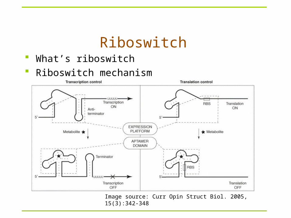
Riboswitch What’s riboswitch Riboswitch mechanism
Image source: Curr Opin Struct Biol. 2005, 15(3):342-348

Structures are more conserved
Structure information is important for alignment (and therefore gene finding)
CGAGCU
CAAGUU

Features of RNA
RNA typically produced as a single stranded molecule (unlike DNA)
Strand folds upon itself to form base pairs & secondary structures
Structure conservation is important
RNA sequence analysis is different from DNA sequence

Canonical base pairing
N N
N
O
H
H
N
N
N
O
H
H
H
N
N
N N
O
O
H
N
N
N
N
N
HH
Watson-Crick base pairingNon-Watson-Crick base pairing G/U (Wobble)

tRNA structure
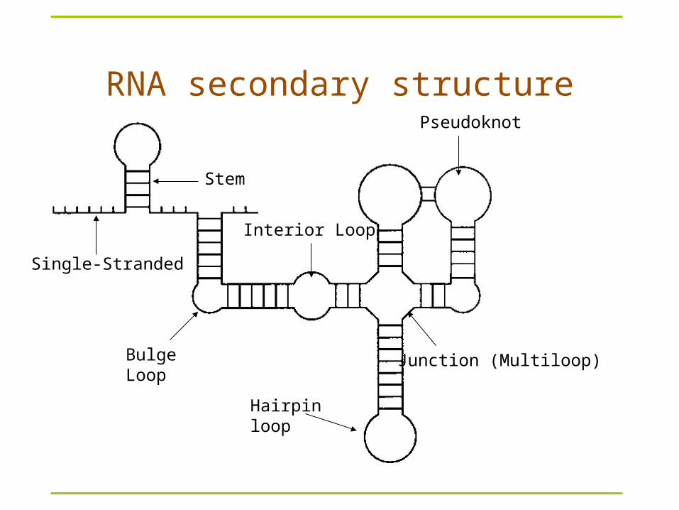
RNA secondary structure
Hairpin loop
Junction (Multiloop)Bulge Loop
Single-Stranded
Interior Loop
Stem
Pseudoknot

Complex folds

Pseudoknots
i
j
j’
i’i j j’i’
?

RNA secondary structure representation
2D Circle plot Dot plot Mountain Parentheses Tree model
(((…)))..((….))

Main approaches to RNA secondary structure prediction
Energy minimization – dynamic programming approach– does not require prior sequence alignment– require estimation of energy terms contributing to
secondary structure Comparative sequence analysis
– using sequence alignment to find conserved residues and covariant base pairs.
– most trusted Simultaneous folding and alignment (structural alignment)

Assumptions in energy minimization approaches
Most likely structure similar to energetically most stable structure
Energy associated with any position is only influenced by local sequence and structure
Neglect pseudoknots
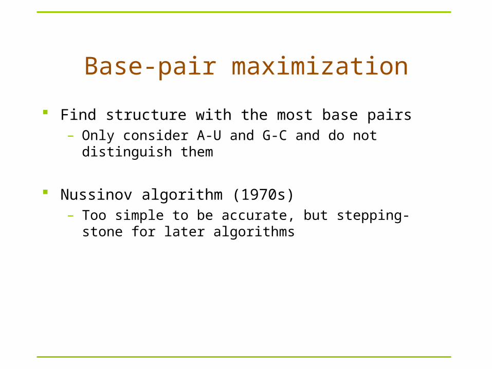
Base-pair maximization
Find structure with the most base pairs– Only consider A-U and G-C and do not distinguish them
Nussinov algorithm (1970s) – Too simple to be accurate, but stepping-stone for later
algorithms

Problem definition– Given sequence X=x1x2…xL,compute a structure that has
maximum (weighted) number of base pairings
How can we solve this problem?– Remember: RNA folds back to itself!– S(i,j) is the maximum score when xi..xj folds optimally– S(1,L)?– S(i,i)?
Nussinov algorithm
1 Li j
S(i,j)
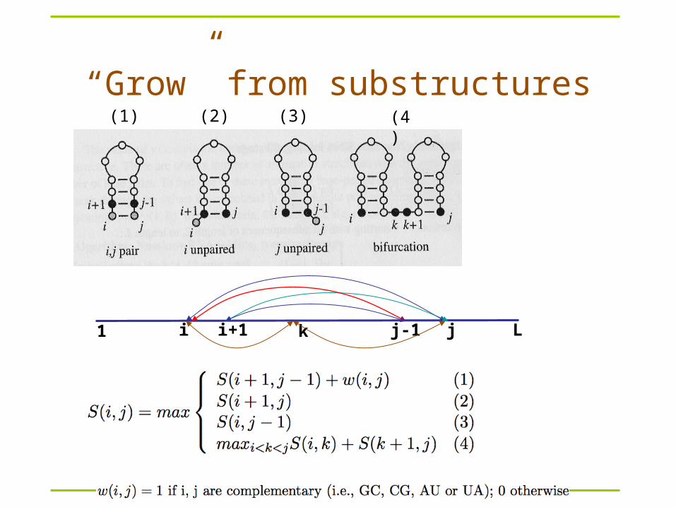
“Grow” from substructures(1) (2) (4)(3)
1 Li ji+1 j-1k
Dynamic programming
Compute S(i,j) recursively (dynamic programming)– Compares a sequence against itself in a dynamic
programming matrix
Three steps
Nussinov RNA Folding Algorithm
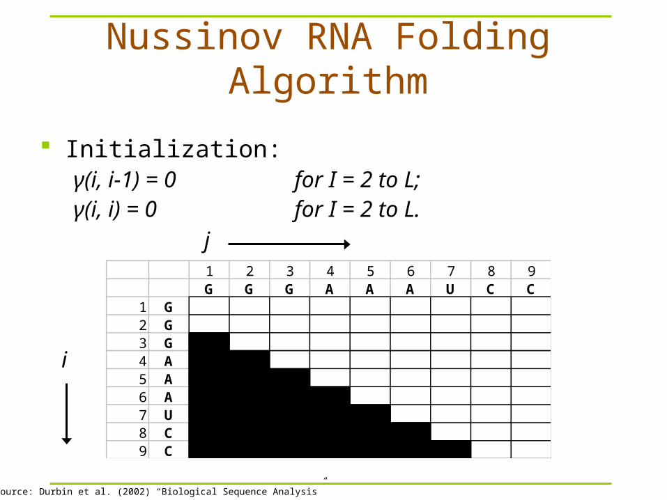
Initialization:γ(i, i-1) = 0 for I = 2 to L;γ(i, i) = 0 for I = 2 to L.
1 2 3 4 5 6 7 8 9G G G A A A U C C
1 G2 G3 G4 A5 A6 A7 U8 C9 C
i
j
Image Source: Durbin et al. (2002) “Biological Sequence Analysis”

Nussinov RNA Folding Algorithm
1 2 3 4 5 6 7 8 9G G G A A A U C C
1 G2 G 03 G 04 A 05 A 06 A 07 U 08 C 09 C 0
j
i
Initialization:γ(i, i-1) = 0 for I = 2 to L;γ(i, i) = 0 for I = 2 to L.
Image Source: Durbin et al. (2002) “Biological Sequence Analysis”

Nussinov RNA Folding Algorithm
1 2 3 4 5 6 7 8 9G G G A A A U C C
1 G 02 G 0 03 G 0 04 A 0 05 A 0 06 A 0 07 U 0 08 C 0 09 C 0 0
j
i
Initialization:γ(i, i-1) = 0 for I = 2 to L;γ(i, i) = 0 for I = 2 to L.
Image Source: Durbin et al. (2002) “Biological Sequence Analysis”

Nussinov RNA Folding Algorithm
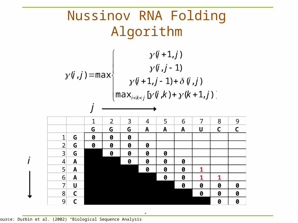
Recursive Relation:
For all subsequences from length 2 to length L:
)],1(),([max
),()1,1(
)1,(
),1(
max),(
jkki
jiji
ji
ji
ji
jki
Case 1
Case 2
Case 3
Case 4

Nussinov RNA Folding Algorithm
1 2 3 4 5 6 7 8 9G G G A A A U C C
1 G 0 02 G 0 0 03 G 0 0 04 A 0 0 05 A 0 0 06 A 0 0 17 U 0 0 08 C 0 0 09 C 0 0
)],1(),([max
),()1,1(
)1,(
),1(
max),(
jkki
jiji
ji
ji
ji
jki
j
i
Image Source: Durbin et al. (2002) “Biological Sequence Analysis”
Nussinov RNA Folding Algorithm
1 2 3 4 5 6 7 8 9G G G A A A U C C
1 G 0 0 02 G 0 0 0 03 G 0 0 0 04 A 0 0 0 05 A 0 0 0 16 A 0 0 1 17 U 0 0 0 08 C 0 0 09 C 0 0
)],1(),([max
),()1,1(
)1,(
),1(
max),(
jkki
jiji
ji
ji
ji
jki
j
i
Image Source: Durbin et al. (2002) “Biological Sequence Analysis”

Nussinov RNA Folding Algorithm
1 2 3 4 5 6 7 8 9G G G A A A U C C
1 G 0 0 0 02 G 0 0 0 0 03 G 0 0 0 0 04 A 0 0 0 0 15 A 0 0 0 1 16 A 0 0 1 1 17 U 0 0 0 08 C 0 0 09 C 0 0
)],1(),([max
),()1,1(
)1,(
),1(
max),(
jkki
jiji
ji
ji
ji
jki
j
i
Image Source: Durbin et al. (2002) “Biological Sequence Analysis”

Example Computation
1 2 3 4 5 6 7 8 9G G G A A A U C C
1 G 0 0 0 02 G 0 0 0 0 03 G 0 0 0 0 04 A 0 0 0 05 A 0 0 0 1 16 A 0 0 1 1 17 U 0 0 0 08 C 0 0 09 C 0 0
j
i
)]7,1(),4([max
)7,4()6,5(
)6,4(
)7,5(
max)7,4(
74 kkk
Image Source: Durbin et al. (2002) “Biological Sequence Analysis”

Example Computation
1 2 3 4 5 6 7 8 9G G G A A A U C C
1 G 0 0 0 02 G 0 0 0 0 03 G 0 0 0 0 04 A 0 0 0 05 A 0 0 0 1 16 A 0 0 1 1 17 U 0 0 0 08 C 0 0 09 C 0 0
j
i
)]7,1(),4([max
)7,4()6,5(
)6,4(
)7,5(
max)7,4(
74 kkk
A U
A
A
i
i+1 j
Image Source: Durbin et al. (2002) “Biological Sequence Analysis”

Example Computation
1 2 3 4 5 6 7 8 9G G G A A A U C C
1 G 0 0 0 02 G 0 0 0 0 03 G 0 0 0 0 04 A 0 0 0 05 A 0 0 0 1 16 A 0 0 1 1 17 U 0 0 0 08 C 0 0 09 C 0 0
j
i
)]7,1(),4([max
)7,4()6,5(
)6,4(
)7,5(
max)7,4(
74 kkk
Image Source: Durbin et al. (2002) “Biological Sequence Analysis”

Example Computation
1 2 3 4 5 6 7 8 9G G G A A A U C C
1 G 0 0 0 02 G 0 0 0 0 03 G 0 0 0 0 04 A 0 0 0 05 A 0 0 0 1 16 A 0 0 1 1 17 U 0 0 0 08 C 0 0 09 C 0 0
j
i
)]7,1(),4([max
)7,4()6,5(
)6,4(
)7,5(
max)7,4(
74 kkk
i+1 j-1
i jA U
A A
Image Source: Durbin et al. (2002) “Biological Sequence Analysis”

Example Computation
1 2 3 4 5 6 7 8 9G G G A A A U C C
1 G 0 0 0 02 G 0 0 0 0 03 G 0 0 0 0 04 A 0 0 0 05 A 0 0 0 1 16 A 0 0 1 1 17 U 0 0 0 08 C 0 0 09 C 0 0
j
i
)]7,1(),4([max
)7,4()6,5(
)6,4(
)7,5(
max)7,4(
74 kkk
Image Source: Durbin et al. (2002) “Biological Sequence Analysis”

Example Computation
1 2 3 4 5 6 7 8 9G G G A A A U C C
1 G 0 0 0 02 G 0 0 0 0 03 G 0 0 0 0 04 A 0 0 0 0 15 A 0 0 0 1 16 A 0 0 1 1 17 U 0 0 0 08 C 0 0 09 C 0 0
j
i
)]7,1(),4([max
)7,4()6,5(
)6,4(
)7,5(
max)7,4(
74 kkk
Image Source: Durbin et al. (2002) “Biological Sequence Analysis”

Completed Matrix
1 2 3 4 5 6 7 8 9G G G A A A U C C
1 G 0 0 0 0 0 0 1 2 32 G 0 0 0 0 0 0 1 2 33 G 0 0 0 0 0 1 2 24 A 0 0 0 0 1 1 15 A 0 0 0 1 1 16 A 0 0 1 1 17 U 0 0 0 08 C 0 0 09 C 0 0
)],1(),([max
),()1,1(
)1,(
),1(
max),(
jkki
jiji
ji
ji
ji
jki
j
i
Image Source: Durbin et al. (2002) “Biological Sequence Analysis”
Traceback
value at γ(1, L) is the total base pair count in the maximally base-paired structure
as in other DP, traceback from γ(1, L) is necessary to recover the final secondary structure
pushdown stack is used to deal with bifurcated structures

Traceback Pseudocode
Initialization: Push (1,L) onto stackRecursion: Repeat until stack is empty: pop (i, j). If i >= j continue; // hit diagonal
else if γ(i+1,j) = γ(i, j) push (i+1,j); // case 1else if γ(i, j-1) = γ(i, j) push (i,j-1); // case 2else if γ(i+1,j-1)+δi,j = γ(i, j): // case 3
record i, j base pairpush (i+1,j-1);
else for k=i+1 to j-1:if γ(i, k)+γ(k+1,j)=γ(i, j): // case 4push (k+1, j).push (i, k).break

Retrieving the Structure
1 2 3 4 5 6 7 8 9G G G A A A U C C
1 G 0 0 0 0 0 0 1 2 32 G 0 0 0 0 0 0 1 2 33 G 0 0 0 0 0 1 2 24 A 0 0 0 0 1 1 15 A 0 0 0 1 1 16 A 0 0 1 1 17 U 0 0 0 08 C 0 0 09 C 0 0
j
i
Image Source: Durbin et al. (2002) “Biological Sequence Analysis”
STACK
(1,9)
CURRENTPAIRS
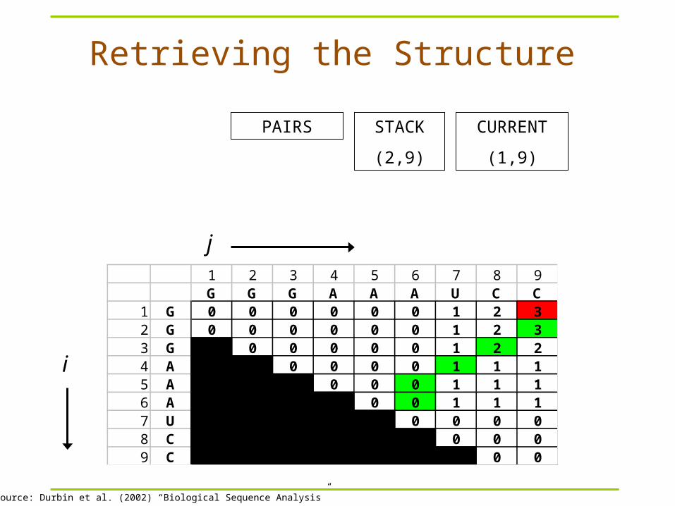
Retrieving the Structure
1 2 3 4 5 6 7 8 9G G G A A A U C C
1 G 0 0 0 0 0 0 1 2 32 G 0 0 0 0 0 0 1 2 33 G 0 0 0 0 0 1 2 24 A 0 0 0 0 1 1 15 A 0 0 0 1 1 16 A 0 0 1 1 17 U 0 0 0 08 C 0 0 09 C 0 0
j
i
Image Source: Durbin et al. (2002) “Biological Sequence Analysis”
STACK
(2,9)
CURRENT
(1,9)
PAIRS

Retrieving the Structure
1 2 3 4 5 6 7 8 9G G G A A A U C C
1 G 0 0 0 0 0 0 1 2 32 G 0 0 0 0 0 0 1 2 33 G 0 0 0 0 0 1 2 24 A 0 0 0 0 1 1 15 A 0 0 0 1 1 16 A 0 0 1 1 17 U 0 0 0 08 C 0 0 09 C 0 0
j
i
Image Source: Durbin et al. (2002) “Biological Sequence Analysis”
STACK
(3,8)
CURRENT
(2,9)
CG
G
PAIRS
(2,9)

Retrieving the Structure
1 2 3 4 5 6 7 8 9G G G A A A U C C
1 G 0 0 0 0 0 0 1 2 32 G 0 0 0 0 0 0 1 2 33 G 0 0 0 0 0 1 2 24 A 0 0 0 0 1 1 15 A 0 0 0 1 1 16 A 0 0 1 1 17 U 0 0 0 08 C 0 0 09 C 0 0
j
i
Image Source: Durbin et al. (2002) “Biological Sequence Analysis”
STACK
(4,7)
CURRENT
(3,8)
CG
GCG
PAIRS
(2,9)
(3,8)

Retrieving the Structure
1 2 3 4 5 6 7 8 9G G G A A A U C C
1 G 0 0 0 0 0 0 1 2 32 G 0 0 0 0 0 0 1 2 33 G 0 0 0 0 0 1 2 24 A 0 0 0 0 1 1 15 A 0 0 0 1 1 16 A 0 0 1 1 17 U 0 0 0 08 C 0 0 09 C 0 0
j
i
Image Source: Durbin et al. (2002) “Biological Sequence Analysis”
STACK
(5,6)
CURRENT
(4,7)U
CG
A
GCG
PAIRS
(2,9)
(3,8)
(4,7)

Retrieving the Structure
1 2 3 4 5 6 7 8 9G G G A A A U C C
1 G 0 0 0 0 0 0 1 2 32 G 0 0 0 0 0 0 1 2 33 G 0 0 0 0 0 1 2 24 A 0 0 0 0 1 1 15 A 0 0 0 1 1 16 A 0 0 1 1 17 U 0 0 0 08 C 0 0 09 C 0 0
j
i
Image Source: Durbin et al. (2002) “Biological Sequence Analysis”
STACK
(6,6)
CURRENT
(5,6)
A
U
CG
A
GCG
PAIRS
(2,9)
(3,8)
(4,7)

Retrieving the Structure
1 2 3 4 5 6 7 8 9G G G A A A U C C
1 G 0 0 0 0 0 0 1 2 32 G 0 0 0 0 0 0 1 2 33 G 0 0 0 0 0 1 2 24 A 0 0 0 0 1 1 15 A 0 0 0 1 1 16 A 0 0 1 1 17 U 0 0 0 08 C 0 0 09 C 0 0
j
i
Image Source: Durbin et al. (2002) “Biological Sequence Analysis”
STACK
-
CURRENT
(6,6)
A
U
CG
A
GCG
A PAIRS
(2,9)
(3,8)
(4,7)

Retrieving the Structure
1 2 3 4 5 6 7 8 9G G G A A A U C C
1 G 0 0 0 0 0 0 1 2 32 G 0 0 0 0 0 0 1 2 33 G 0 0 0 0 0 1 2 24 A 0 0 0 0 1 1 15 A 0 0 0 1 1 16 A 0 0 1 1 17 U 0 0 0 08 C 0 0 09 C 0 0
j
i
A
U
CG
A
GCG
A
Image Source: Durbin et al. (2002) “Biological Sequence Analysis”
Evaluation of Nussinov
unfortunately, while this does maximize the base pairs, it does not create viable secondary structures
in Zuker’s algorithm, the correct structure is assumed to have the lowest equilibrium free energy (ΔG) (Zuker and Stiegler, 1981; Zuker 1989a)

Free energy computation U U A A G C G C A G C U A A U C G A U A 3’A5’
-0.3
-0.3
-1.1 mismatch of hairpin-2.9 stacking
+3.3 1nt bulge -2.9 stacking
-1.8 stacking
5’ dangling
-0.9 stacking -1.8 stacking
-2.1 stacking
G = -4.6 KCAL/MOL
+5.9 4nt loop

Loop parameters(from Mfold)
Unit: Kcal/mol
DESTABILIZING ENERGIES BY SIZE OF LOOP SIZE INTERNAL BULGE HAIRPIN-------------------------------------------------------1 . 3.8 .2 . 2.8 .3 . 3.2 5.44 1.1 3.6 5.65 2.1 4.0 5.76 1.9 4.4 5.4..12 2.6 5.1 6.713 2.7 5.2 6.814 2.8 5.3 6.915 2.8 5.4 6.9

Stacking energy(from Vienna package)
# stack_energies/* CG GC GU UG AU UA @ */ -2.0 -2.9 -1.9 -1.2 -1.7 -1.8 0 -2.9 -3.4 -2.1 -1.4 -2.1 -2.3 0 -1.9 -2.1 1.5 -.4 -1.0 -1.1 0 -1.2 -1.4 -.4 -.2 -.5 -.8 0 -1.7 -.2 -1.0 -.5 -.9 -.9 0 -1.8 -2.3 -1.1 -.8 -.9 -1.1 0 0 0 0 0 0 0 0

Mfold versus Vienna package
Mfold– http://frontend.bioinfo.rpi.edu/zukerm/download/– http://frontend.bioinfo.rpi.edu/applications/mfold/cgi-bin/rna-f
orm1.cgi– Suboptimal structures
• The correct structure is not necessarily structure with optimal free energy
• Within a certain threshold of the calculated minimum energy
Vienna -- calculate the probability of base pairings– http://www.tbi.univie.ac.at/RNA/

Mfold energy dot plot

Mfold algorithm(Zuker & Stiegler, NAR 1981 9(1):133)

A Context Free Grammar
S AB Nonterminals: S, A, BA aAc | a Terminals: a, b, c, dB bBd | b
Derivation:
S AB aAcB … aaaacccB aaaacccbBd … aaaacccbbbbbbddd
Produces all strings ai+1cibj+1dj, for i, j 0
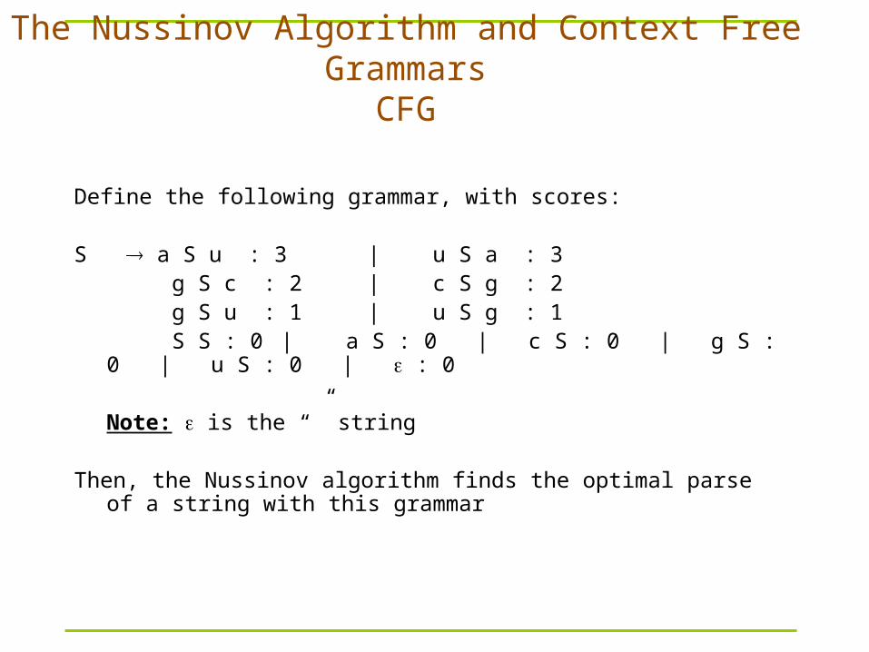
The Nussinov Algorithm and Context Free GrammarsCFG
Define the following grammar, with scores:
S a S u : 3 | u S a : 3 g S c : 2 | c S g : 2 g S u : 1 | u S g : 1 S S : 0 | a S : 0 | c S : 0 | g S : 0 | u S : 0 | : 0
Note: is the “” string
Then, the Nussinov algorithm finds the optimal parse of a string with this grammar

Example: modeling a stem loop
S a W1 u
W1 c W2 g
W2 g W3 c
W3 g L c
L agucg
What if the stem loop can have other letters in place of the ones shown?
ACGGUGCC
AG UCG

Example: modeling a stem loop
S a W1 u | g W1 u
W1 c W2 g
W2 g W3 c | g W3 u
W3 g L c | a L uL agucg | agccg | cugugc
More general: Any 4-long stem, 3-5-long loop:
S aW1u | gW1u | gW1c | cW1g | uW1g | uW1a
W1 aW2u | gW2u | gW2c | cW2g | uW2g | uW2a
W2 aW3u | gW3u | gW3c | cW3g | uW3g | uW3a
W3 aLu | gLu | gLc | cLg | uLg | uLa
L aL1 | cL1 | gL1 | uL1
L1 aL2 | cL2 | gL2 | uL2
L2 a | c | g | u | aa | … | uu | aaa | … | uuu
ACGGUGCC
AG UCG
GCGAUGCU
AG CCG
GCGAUGUU
CUG UCG
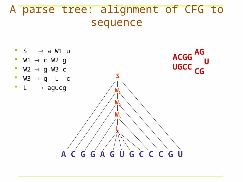
A parse tree: alignment of CFG to sequence
ACGGUGCC
AG UCG
A C G G A G U G C C C G U
S
W1
W2
W3
L
S a W1 u W1 c W2 g W2 g W3 c W3 g L c L agucg

Alignment scores for parses
We can define each rule X s, where s is a string,
to have a score.
Example:
W a W’ u: 3 (forms 3 hydrogen bonds)
W g W’ c: 2 (forms 2 hydrogen bonds)
W g W’ u: 1 (forms 1 hydrogen bond)
W x W’ z -1, when (x, z) is not an a/u, g/c, g/u pair
Questions:- How do we best align a CFG to a sequence: DP- How do we set the parameters: Stochastic CFGs.

The Nussinov AlgorithmInitialization:
F(i, i-1) = 0; for i = 2 to N
F(i, i) = 0; for i = 1 to N S a | c | g | u
Iteration:
For i = 2 to N:
For i = 1 to N – l
j = i + L – 1
F(i+1, j -1) + s(xi, xj) S a S u | …
F(i, j) = max
max{ i k < j } F(i, k) + F(k+1, j) S S S
Termination:
Best structure is given by F(1, N)

Stochastic Context Free Grammars
In an analogy to HMMs, we can assign probabilities to transitions:
Given grammar
X1 s11 | … | sin
…
Xm sm1 | … | smn
Can assign probability to each rule, s.t.
P(Xi si1) + … + P(Xi sin) = 1

Computational Problems
Calculate an optimal alignment of a sequence and a SCFG
(DECODING)
Calculate Prob[ sequence | grammar ]
(EVALUATION)
Given a set of sequences, estimate parameters of a SCFG
(LEARNING)

Normal Forms for CFGs
Chomsky Normal Form:
X YZ
X a
All productions are either to 2 nonterminals, or to 1 terminal
Theorem (technical)
Every CFG has an equivalent one in Chomsky Normal Form
(That is, the grammar in normal form produces exactly the same set of strings)

Example of converting a CFG to C.N.F.
S ABCA Aa | aB Bb | bC CAc | c
Converting:
S AS’S’ BCA AA | aB BB | bC DC’ | cC’ cD CA
S
A B C
A a
a
B b
B b
b
C A c
c a
S
A S ’
B CA A
a a B B
B B
b b
b
D C ’
C A c
c a

Another example
S ABCA C | aAB bB | bC cCd | c
Converting:S AS’S’ BCA C’C’’ | c | A’AA’ aB B’B | bB’ bC C’C’’ | cC’ cC’’ CDD d

Decoding: the CYK algorithm
Given x = x1....xN, and a SCFG G,
Find the most likely parse of x
(the most likely alignment of G to x)
Dynamic programming variable:
(i, j, V): likelihood of the most likely parse of xi…xj,
rooted at nonterminal V
Then,
(1, N, S): likelihood of the most likely parse of x by the grammar

The CYK algorithm (Cocke-Younger-Kasami)
Initialization:For i = 1 to N, any nonterminal V,
(i, i, V) = log P(V xi)
Iteration:For i = 1 to N-1 For j = i+1 to N For any nonterminal V,
(i, j, V) = maxXmaxYmaxik<j (i,k,X) + (k+1,j,Y) + log P(VXY)
Termination:log P(x | , *) = (1, N, S)
Where * is the optimal parse tree (if traced back appropriately from above)

A SCFG for predicting RNA structure
S a S | c S | g S | u S | S a | S c | S g | S u
a S u | c S g | g S u | u S g | g S c | u S a
SS
Adjust the probability parameters to reflect bond strength etc
No distinction between non-paired bases, bulges, loops Can modify to model these events
– L: loop nonterminal
– H: hairpin nonterminal
– B: bulge nonterminal
– etc

CYK for RNA folding
Initialization:
(i, i-1) = log P()
Iteration:
For i = 1 to N
For j = i to N
(i+1, j–1) + log P(xi S xj)
(i, j–1) + log P(S xi)
(i, j) = max
(i+1, j) + log P(xi S)
maxi < k < j (i, k) + (k+1, j) + log P(S S)

Evaluation
Recall HMMs:
Forward: fl(i) = P(x1…xi, i = l)
Backward: bk(i) = P(xi+1…xN | i = k)
Then,
P(x) = k fk(N) ak0 = l a0l el(x1) bl(1)
Analogue in SCFGs:
Inside: a(i, j, V) = P(xi…xj is generated by nonterminal V)
Outside: b(i, j, V) = P(x, excluding xi…xj is generated by S and the excluded part is rooted at V)

The Inside Algorithm
To compute
a(i, j, V) = P(xi…xj, produced by V)
a(i, j, v) = X Y k a(i, k, X) a(k+1, j, Y) P(V XY)
k k+1i j
V
X Y
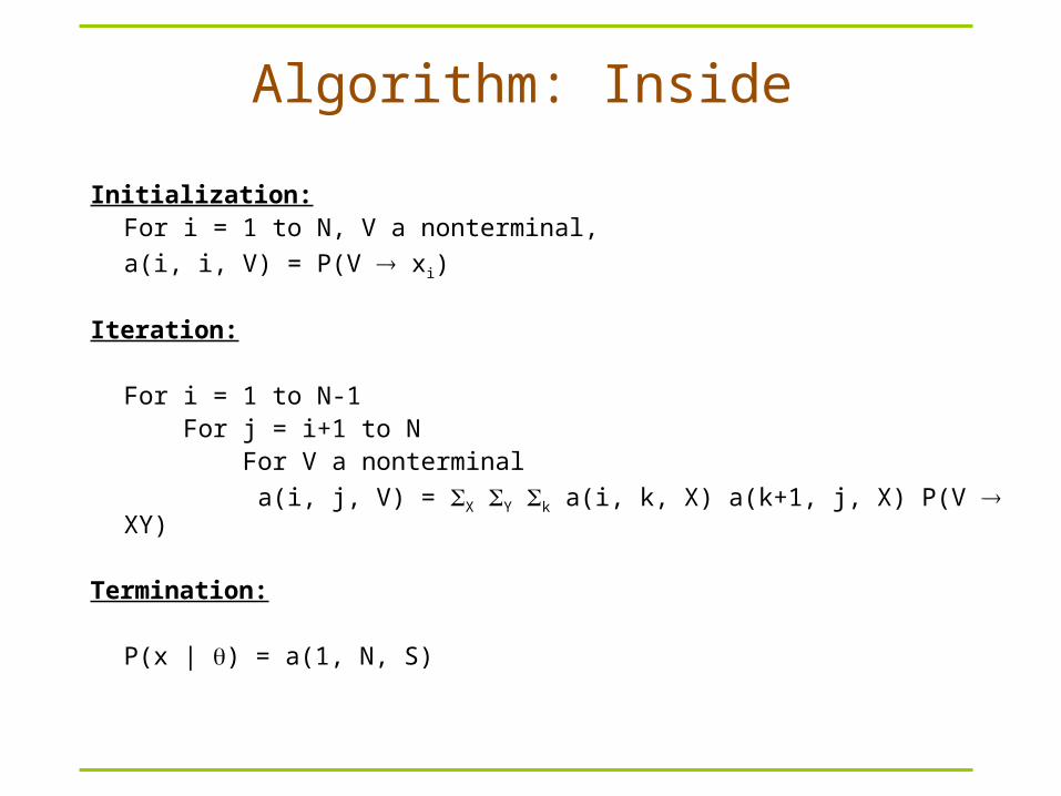
Algorithm: Inside
Initialization:For i = 1 to N, V a nonterminal,
a(i, i, V) = P(V xi)
Iteration:
For i = 1 to N-1 For j = i+1 to N For V a nonterminal
a(i, j, V) = X Y k a(i, k, X) a(k+1, j, X) P(V XY)
Termination:
P(x | ) = a(1, N, S)

The Outside Algorithm
b(i, j, V) = Prob(x1…xi-1, xj+1…xN, where the “gap” is rooted at V)
Given that V is the right-hand-side nonterminal of a production,
b(i, j, V) = X Y k<i a(k, i-1, X) b(k, j, Y) P(Y XV)
i j
V
k
X
Y

Algorithm: Outside
Initialization:b(1, N, S) = 1For any other V, b(1, N, V) = 0
Iteration:
For i = 1 to N-1 For j = N down to i For V a nonterminal
b(i, j, V) = X Y k<i a(k, i-1, X) b(k, j, Y) P(Y XV) +
X Y k<i a(j+1, k, X) b(i, k, Y) P(Y VX)
Termination:It is true for any i, that:
P(x | ) = X b(i, i, X) P(X xi)

Learning for SCFGs
We can now estimate
c(V) = expected number of times V is used in the parse of x1….xN
1
c(V) = –––––––– 1iNijN a(i, j, V) b(i, j, v)
P(x | )
1
c(VXY) = –––––––– 1iNi<jN ik<j b(i,j,V) a(i,k,X) a(k+1,j,Y) P(VXY)
P(x | )

Learning for SCFGs
Then, we can re-estimate the parameters with EM, by:
c(VXY)
Pnew(VXY) = ––––––––––––
c(V)
c(V a) i: xi = a b(i, i, V) P(V a)
Pnew(V a) = –––––––––– = ------------------------------------------
c(V) 1iNi<jN a(i, j, V) b(i, j, V)

Summary: SCFG and HMM algorithms
GOAL HMM algorithm SCFG algorithm
Optimal parse Viterbi CYK
Estimation Forward InsideBackward Outside
Learning EM: Fw/Bck EM: Ins/Outs
Memory Complexity O(N K) O(N2 K)Time Complexity O(N K2) O(N3 K3)
Where K: # of states in the HMM # of nonterminals in the SCFG

Methods for inferring RNA fold
Experimental: – Crystallography– NMR
Computational– Fold prediction (Nussinov, Zuker, SCFGs)– Multiple Alignment

Multiple alignment and RNA folding
Given K homologous aligned RNA sequences:
Human aagacuucggaucuggcgacaccc
Mouse uacacuucggaugacaccaaagug
Worm aggucuucggcacgggcaccauuc
Fly ccaacuucggauuuugcuaccaua
Orc aagccuucggagcgggcguaacuc
If ith and jth positions are always base paired and covary, then they are likely to be paired

Mutual information
: frequency of a base in column i
: joint (pairwise) frequency of a base pair between columns i and j
Information ranges from 0 and ? bits
If i and j are uncorrelated (independent), mutual information is 0
Mutual information
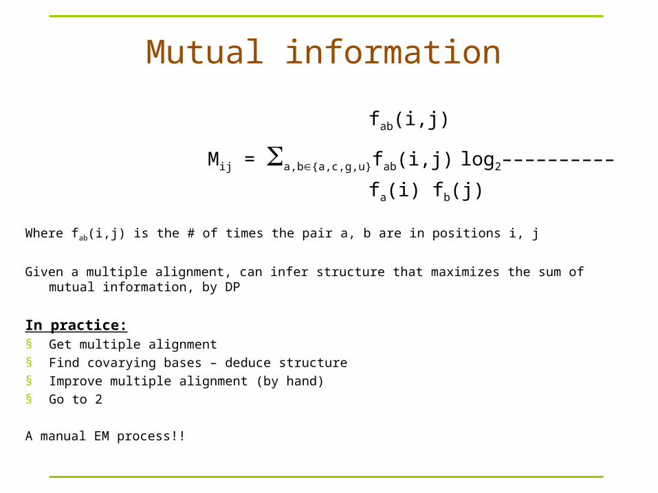
fab(i,j)
Mij = a,b{a,c,g,u}fab(i,j) log2––––––––––
fa(i) fb(j)
Where fab(i,j) is the # of times the pair a, b are in positions i, j
Given a multiple alignment, can infer structure that maximizes the sum of mutual information, by DP
In practice:§ Get multiple alignment§ Find covarying bases – deduce structure§ Improve multiple alignment (by hand)§ Go to 2
A manual EM process!!

Inferring structure by comparative sequence analysis
Need a multiple sequence alignment as input
Requires sequences be similar enough (so that they can be initially aligned)
Sequences should be dissimilar enough for covarying substitutions to be detected
“Given an accurate multiple alignment, a large number of
sequences, and sufficient sequence diversity, comparative analysis alone is sufficient to produce accurate structure predictions” (Gutell RR et al. Curr Opin Struct Biol 2002, 12:301-310)

RNA variations Variations in RNA sequence maintain base-pairing patterns
for secondary structures (conserved patterns of base-pairing)
When a nucleotide in one base changes, the base it pairs to must also change to maintain the same structure
Such variation is referred to as covariation.
CGAGCU
CAAGUU

If neglect covariation
In usual alignment algorithms they are doubly penalized
…GA…UC……GA…UC……GA…UC……GC…GC……GA…UA…

Covariance measurements Mutual information (desirable for large datasets)
– Most common measurement– Used in CM (Covariance Model) for structure prediction
Covariance score (better for small datasets)
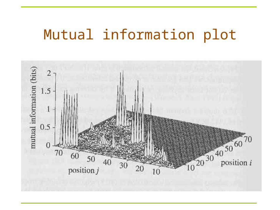
Mutual information plot

Structure prediction using MI S(i,j) = Score at indices i and j; M(i,j) is the mutual information between i and j The goal is to maximize the total mutual information of input RNA The recursion is just like the one in Nussinov Algorithm, just to replace w(i,j) (1 or 0) with the mutual
information M(i,j)

Covariance-like score
RNAalifold– Hofacker et al. JMB 2002, 319:1059-1066
Desirable for small datasets Combination of covariance score and
thermodynamics energy

Covariance-like score calculationThe score between two columns i and j of an input multiple alignment is computed as following:

Covariance model A formal covariance model, CM, devised by
Eddy and Durbin– A probabilistic model– ≈ A Stochastic Context-Free Grammer– Generalized HMM model
A CM is like a sequence profile, but it scores a combination of sequence consensus and RNA secondary structure consensus
Provides very accurate results Very slow and unsuitable for searching large
genomes

CM training algorithm
Unaligned sequence
Modeling construction
EMMultiple alignment
alignment
Parameter re-estimation
Covariance model
Binary tree representation of RNA secondary structure
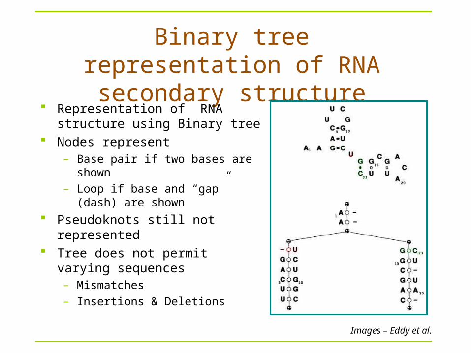
Representation of RNA structure using Binary tree
Nodes represent– Base pair if two bases are shown
– Loop if base and “gap” (dash) are shown
Pseudoknots still not represented Tree does not permit varying
sequences– Mismatches
– Insertions & Deletions
Images – Eddy et al.

Overall CM architecture
MATP emits pairs of bases: modeling of base pairing
BIF allows multiple helices (bifurcation)

Covariance model drawbacks
Needs to be well trained (large datasets) Not suitable for searches of large RNA
– Structural complexity of large RNA cannot be modeled
– Runtime– Memory requirements
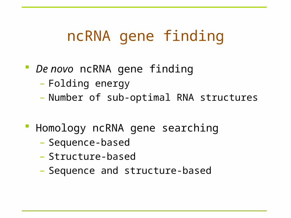
ncRNA gene finding
De novo ncRNA gene finding– Folding energy– Number of sub-optimal RNA structures
Homology ncRNA gene searching– Sequence-based– Structure-based– Sequence and structure-based

Rfam & Infernal Rfam 9.1 contains 1379 families (December 2008) Rfam 10.0 contains 1446 families (January 2010) Rfam is a collection of multiple sequence
alignments and covariance models covering many common non-coding RNA families
Infernal searches Rfam covariance models (CMs) in genomes or other DNA sequence databases for homologs to known structural RNA families
http://rfam.janelia.org/

An example of Rfam families
TPP (a riboswitch; THI element)– RF00059– is a riboswitch that directly binds to TPP (active
form of VB, thiamin pyrophosphate) to regulate gene expression through a variety of mechanisms in archaea, bacteria and eukaryotes

Simultaneous structure prediction
and alignment of ncRNAs
http://www.biomedcentral.com/1471-2105/7/400
The grammar emits two correlated sequences, x and y
References How Do RNA Folding Algorithms Work? Eddy. Nature Biotechnology,
22:1457-1458, 2004 (a short nice review) Biological Sequence Analysis: Probabilistic models of proteins and
nucleic acids. Durbin, Eddy, Krogh and Mitchison. 1998 Chapter 10, pages 260-297
Secondary Structure Prediction for Aligned RNA Sequences. Hofacker et al. JMB, 319:1059-1066, 2002 (RNAalifold; covariance-like score calculation)
Optimal Computer Folding of Large RNA Sequences Using Thermodynamics and Auxiliary Information. Zuker and Stiegler. NAR, 9(1):133-148, 1981 (Mfold)
A computational pipeline for high throughput discovery of cis-regulatory noncoding RNAs in Bacteria, PLoS CB 3(7):e126
– Riboswitches in Eubacteria Sense the Second Messenger Cyclic Di-GMP, Science, 321:411 – 413, 2008
– Identification of 22 candidate structured RNAs in bacteria using the CMfinder comparative genomics pipeline, Nucl. Acids Res. (2007) 35 (14): 4809-4819.
– CMfinder—a covariance model based RNA motif finding algorithm. Bioinformatics 2006;22:445-452

Understanding the transcriptome through RNA structure
'RNA structurome’ Genome-wide measurements of RNA structure
by high-throughput sequencing
Nat Rev Genet. 2011 Aug 18;12(9):641-55