RMSD and Symmetry

Evangelos A. Coutsias∗, Michael J. Wester†

February 8, 2019

Abstract

A common approach for comparing the structures of biomolecules or solid bod-ies is to translate and rotate one structure with respect to the other to minimizethe pointwise root-mean-square deviation (RMSD). We present a new, robust nu-merical algorithm that computes the RMSD between two molecules or all the mu-tual RMSDs of a list of molecules and, if desired, the corresponding rotation ma-trix in a minimal number of operations as compared to previous algorithms. TheRMSD gradient can also be computed. We address the problem of symmetry, bothin alignment (possible alternative alignments due to indistinguishable atoms) as wellas geometry. In the latter case, it is possible to have degenerate superposition. Anecessary condition is optimal superimposability to one’s mirror image. Double (re-spectively, triple) degeneracy results in a 1- (respectively, 2)-parameter family of ro-tations leaving the superposition invariant. The software, frmsd, is freely available athttp://www.ams.stonybrook.edu/∼coutsias/codes/frmsd.tgz.

Keywords: optimal superposition, alignment, symmetry, chirality, degeneracy.

∗Department of Applied Mathematics and Statistics and Laufer Center for Physical and QuantitativeBiology, Stony Brook University, Stony Brook, New York 11794†Department of Mathematics and Statistics, University of New Mexico, Albuquerque, New Mexico 87131

1

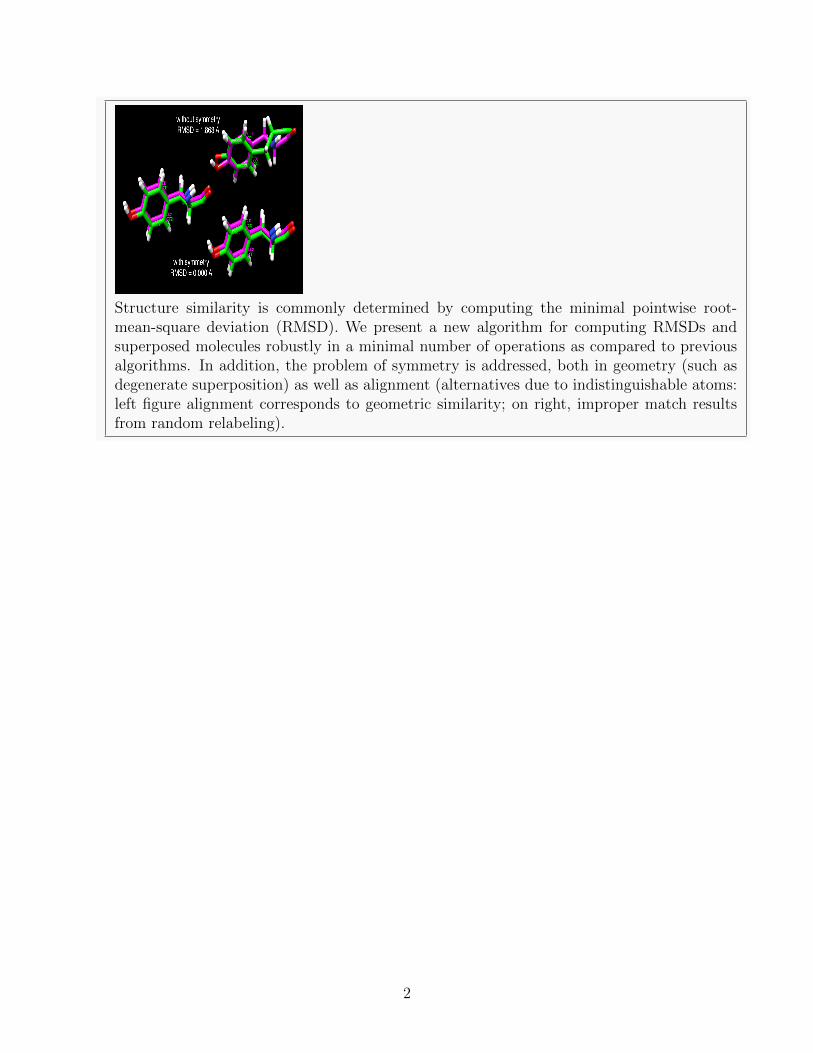
Structure similarity is commonly determined by computing the minimal pointwise root-mean-square deviation (RMSD). We present a new algorithm for computing RMSDs andsuperposed molecules robustly in a minimal number of operations as compared to previousalgorithms. In addition, the problem of symmetry is addressed, both in geometry (such asdegenerate superposition) as well as alignment (alternatives due to indistinguishable atoms:left figure alignment corresponds to geometric similarity; on right, improper match resultsfrom random relabeling).

2

INTRODUCTION

The Root Mean Squared Distance (RMSD) is one of the most commonly used expressions

for the structural (dis)similarity between two conformations of a molecule. The calculation

of the RMSD involves two main steps: (i) alignment and (ii) optimal superposition. Aligning

two conformations means establishing a 1-1 correspondence between equivalent atoms in each

conformation. Optimal superposition is found by rotating and translating one structure so

that the weighted sum of the squares of the distances between equivalent atoms in the two

structures is minimized. The optimal translation simply superimposes the barycenters of

the two point sets, while the optimal rotation requires solving a 4×4 eigenvalue problem for

the quaternion giving the optimal rotation about the common barycenter1. Alternatively a

method based on the SVD of a 3× 3 matrix may be employed2.

Most available algorithms for the computation of RMSD assume a pre-existing 1-1 align-

ment among pairs of points on the two objects. For typical RMSD calculations between

pairs of protein structures, a Cα-based backbone RMSD computation may proceed regard-

less of specific sequence composition, simply on the basis of identical chain lengths for the

two proteins under comparison, aligning atoms based on similar residue indices. However, in

sidechain refinement comparisons involving all-heavy atoms in a protein or in applications

such as docking in which the details of sidechain placement are critical for contact formation,

symmetry matching must be considered, where certain ring structures or atoms at the ends

of certain sidechains may introduce classes of valid alternative alignments. These alterna-

tives arise by noting that the labeling of indistinguishable atoms is arbitrary, resulting in

non-unique RMSD assignments. For example, the ε oxygens in a glutamic acid residue are

indistinguishable. Similarly, in comparing two different conformations of a tyrosine residue,

two distinct alignments involving indistinguishable ring atoms will generally result in two

different RMSD values. Clearly, all-heavy atom RMSD comparisons for proteins are not

relevant unless such residue symmetries are fully accounted for3. This becomes even more

serious in comparisons of other complex molecules composed of indistinguishable sub-units,

arranged in a symmetric graph. Clearly, the alignment giving the lowest RMSD must be

considered in each case.

3

The mathematical statement of the basic problem (presupposing an alignment and having

both point-sets shifted to barycentric coordinates for simplicity) is:

Given an ordered set of vectors yk (target) and a second set xk (model), 1 ≤ k ≤ N , both

having barycenters at the origin, find an orthogonal transformation U such that the residual

E (weighted by wk)

E :=1

N

N∑k=1

wk|Uxk − yk|2 (1)

is minimized. The weight factor wk permits emphasizing various parts of the structure, such

as the backbone of a polypeptide. Often, the weights will be equal to one. Since the weights

can be incorporated into xk and yk, we omit wk below.

Two direct methods are known for computing the RMSD after conversion to barycentric

coordinates. The first, commonly referred to as the SVD method2 (or Kabsch’s method4),

computes the RMSD in terms of the singular values of a 3 × 3 matrix, while the second,

based on quaternions, finds the RMSD in terms of the largest eigenvalue of a symmetric,

traceless 4 × 4 matrix5,6. In the latter case, the optimal superposition is expressed by the

leading eigenvector, viewed as a unit quaternion.

Several algorithms exist for the efficient computation of the RMSD. We mention but a

few: Tietze5, Kearsley6, Kneller7, Coutsias et al.1, Theobald and Liu et al.8–10. In previous

works1,11, we proved the mathematical equivalence between the SVD and quaternion meth-

ods. A survey of the extensive related literature was presented there and we refer the reader

to it.

The most efficient algorithm for computing the RMSD (and rotation) to date appears

to be the approach suggested by Theobald8 as implemented in the algorithm qrmsd9: since

the 4× 4 matrix is symmetric and traceless, its largest eigenvalue can be robustly computed

from the characteristic polynomial using a Newton iteration; once the eigenvalue is known to

adequate precision, the corresponding eigenvector can be computed. From the eigenvector,

the optimal rotation, presented as either a quaternion or a rotation matrix, can then be

easily produced.

In this note, we show how to achieve an additional, substantial speedup by taking advan-

tage of the algebraic equivalence between the SVD and quaternion approaches. In1 simple

4

formulas were found, relating the coefficients of the characteristic polynomial of the 4 × 4

matrix that appears in the quaternion method to the coefficients of the characteristic poly-

nomial of the 3 × 3 matrix appearing in the SVD method (the latter is the resolvent cubic

of the former). In this paper we present a new algorithm, frmsd, that exploits this corre-

spondence to substantially reduce the operation count involved in the RMSD computation.

Our algorithm, like that of Theobald8 and Liu et al.9, is based on solving the characteristic

polynomial for the largest eigenvalue. The main differences are: the use of the equivalent

cubic formulation in1 to arrive at more compact forms of the polynomial coefficients; and

the use of symmetric maximal pivoting for finding the corresponding eigenvector efficiently

and stably, again in a minimum of operations as compared to the approach used in Liu et

al.9, even when degeneracy is present. We demonstrate the speed of frmsd by comparison to

qrmsd9 in Supporting Information A.

An important feature of our algorithm is that it is designed to efficiently compare large

numbers of molecules, for example, all the molecules in a list with either the first or with each

other, so conversion to barycentric coordinates is done initially for all molecules. Further-

more, the algorithm allows for encoding indistinguishable atom equivalence and incorporates

an efficient combinatoric search through a table of pre-specified symmetries to discover the

alignment producing the minimal RMSD between two structures, with matrix recalculation

involving only the transposed atoms. It has been been argued3 that for molecules of more

than ≈ 100 atoms, e.g., for all-heavy atom RMSD calculations for even small proteins, the

dominant part of the operational cost is the setup of the 4× 4 RMSD matrix, overwhelming

the rest of the calculation. However, as Figure 3 shows, accounting for residue symmetries

in most cases alters that picture, making the search for the optimal alignment the dominant

part, provided the matrix setup is optimized against redundancy. We demonstrate in Fig-

ure 4 the effect of accounting for sidechain symmetries in a high-resolution decoy-set based

on all-heavy atom comparisons.

Besides alignment symmetries, our implementation takes care of structural symmetry

as well: existence of degeneracy may indicate geometric symmetry. Indeed, if the leading

positive eigenvalue is degenerate, then there is a continuum of superpositions that results

in identical optimal RMSDs. As the 4 × 4 matrix is traceless, a degeneracy in the leading

5

positive eigenvalue implies that the most negative eigenvalue must be of greater absolute

value (or, equal if also degenerate). Thus, a necessary condition for such degeneracy is that

the enantiomeric superposition is optimal, so that a mirror image of one structure has a

better fit with the other structure. The calculation of eigenvectors presented here is capable

of detecting doubly or triply degenerate leading eigenvalues and of adapting the leading

eigenspace calculation accordingly. Our method takes advantage of the special structure of

the quaternion based eigenproblem by first performing symmetric pivoted Gauss elimination

to robustly reduce the system size, and then by considering a judiciously chosen set of minors

to complete the calculation while detecting the possibility of degeneracy. Thus, our algorithm

is guaranteed to complete in all cases. In this context, we will exhibit examples of degenerate

superposition. Our algorithm is publicly available under an open source BSD license at

http://www.ams.stonybrook.edu/∼coutsias/codes/frmsd.tgz.

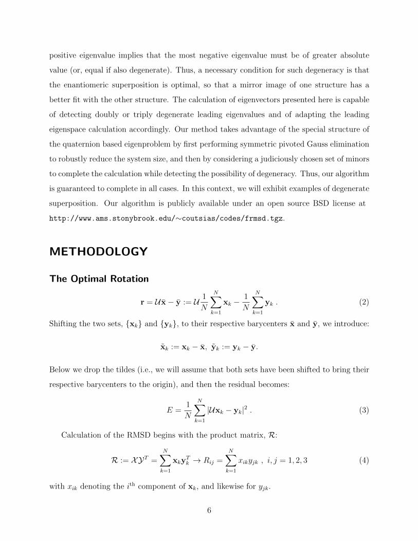
METHODOLOGY

The Optimal Rotation

r = U x− y := U 1

N

N∑k=1

xk −1

N

N∑k=1

yk . (2)

Shifting the two sets, {xk} and {yk}, to their respective barycenters x and y, we introduce:

xk := xk − x, yk := yk − y.

Below we drop the tildes (i.e., we will assume that both sets have been shifted to bring their

respective barycenters to the origin), and then the residual becomes:

E =1

N

N∑k=1

|Uxk − yk|2 . (3)

Calculation of the RMSD begins with the product matrix, R:

R := XYT =N∑k=1

xkyTk → Rij =

N∑k=1

xikyjk , i, j = 1, 2, 3 (4)

with xik denoting the ith component of xk, and likewise for yjk.

6

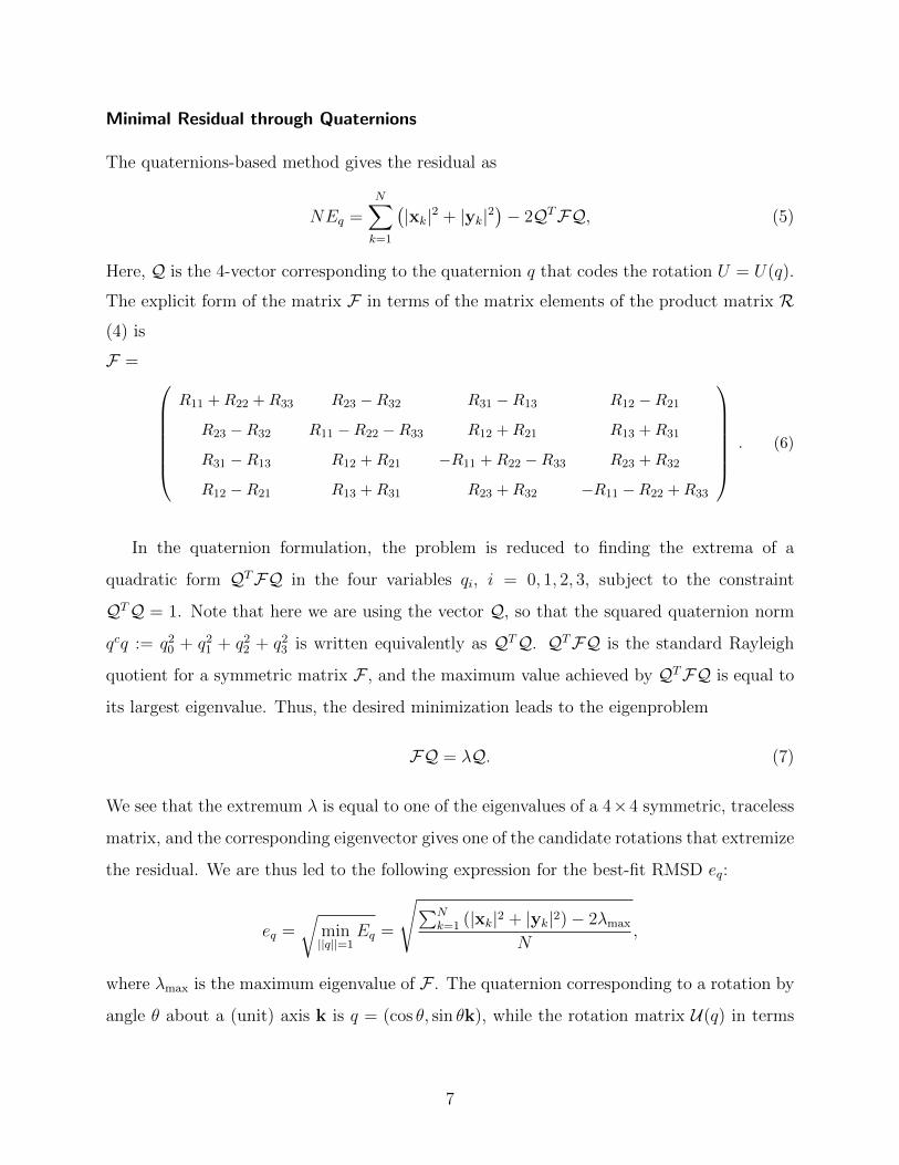
Minimal Residual through Quaternions

The quaternions-based method gives the residual as

NEq =N∑k=1

(|xk|2 + |yk|2

)− 2QTFQ, (5)

Here, Q is the 4-vector corresponding to the quaternion q that codes the rotation U = U(q).

The explicit form of the matrix F in terms of the matrix elements of the product matrix R(4) is

F = R11 + R22 + R33 R23 −R32 R31 −R13 R12 −R21

R23 −R32 R11 −R22 −R33 R12 + R21 R13 + R31

R31 −R13 R12 + R21 −R11 + R22 −R33 R23 + R32

R12 −R21 R13 + R31 R23 + R32 −R11 −R22 + R33

. (6)

In the quaternion formulation, the problem is reduced to finding the extrema of a

quadratic form QTFQ in the four variables qi, i = 0, 1, 2, 3, subject to the constraint

QTQ = 1. Note that here we are using the vector Q, so that the squared quaternion norm

qcq := q20 + q2

1 + q22 + q2

3 is written equivalently as QTQ. QTFQ is the standard Rayleigh

quotient for a symmetric matrix F , and the maximum value achieved by QTFQ is equal to

its largest eigenvalue. Thus, the desired minimization leads to the eigenproblem

FQ = λQ. (7)

We see that the extremum λ is equal to one of the eigenvalues of a 4×4 symmetric, traceless

matrix, and the corresponding eigenvector gives one of the candidate rotations that extremize

the residual. We are thus led to the following expression for the best-fit RMSD eq:

eq =√

min||q||=1

Eq =

√∑Nk=1 (|xk|2 + |yk|2)− 2λmax

N,

where λmax is the maximum eigenvalue of F . The quaternion corresponding to a rotation by

angle θ about a (unit) axis k is q = (cos θ, sin θk), while the rotation matrix U(q) in terms

7

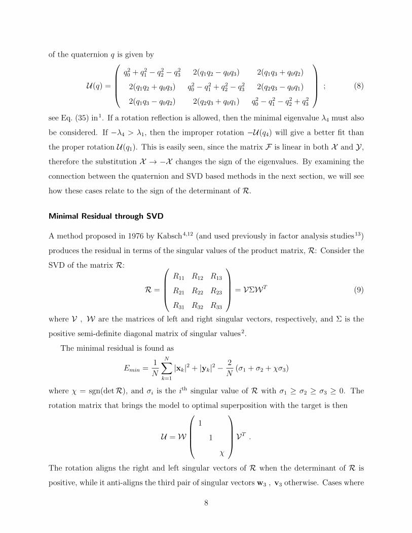
of the quaternion q is given by

U(q) =

q2

0 + q21 − q2

2 − q23 2(q1q2 − q0q3) 2(q1q3 + q0q2)

2(q1q2 + q0q3) q20 − q2

1 + q22 − q2

3 2(q2q3 − q0q1)

2(q1q3 − q0q2) 2(q2q3 + q0q1) q20 − q2

1 − q22 + q2

3

; (8)

see Eq. (35) in1. If a rotation reflection is allowed, then the minimal eigenvalue λ4 must also

be considered. If −λ4 > λ1, then the improper rotation −U(q4) will give a better fit than

the proper rotation U(q1). This is easily seen, since the matrix F is linear in both X and Y ,

therefore the substitution X → −X changes the sign of the eigenvalues. By examining the

connection between the quaternion and SVD based methods in the next section, we will see

how these cases relate to the sign of the determinant of R.

Minimal Residual through SVD

A method proposed in 1976 by Kabsch4,12 (and used previously in factor analysis studies13)

produces the residual in terms of the singular values of the product matrix, R: Consider the

SVD of the matrix R:

R =

R11 R12 R13

R21 R22 R23

R31 R32 R33

= VΣWT (9)

where V , W are the matrices of left and right singular vectors, respectively, and Σ is the

positive semi-definite diagonal matrix of singular values2.

The minimal residual is found as

Emin =1

N

N∑k=1

|xk|2 + |yk|2 −2

N(σ1 + σ2 + χσ3)

where χ = sgn(detR), and σi is the ith singular value of R with σ1 ≥ σ2 ≥ σ3 ≥ 0. The

rotation matrix that brings the model to optimal superposition with the target is then

U =W

1

1

χ

VT .The rotation aligns the right and left singular vectors of R when the determinant of R is

positive, while it anti-aligns the third pair of singular vectors w3 , v3 otherwise. Cases where

8

an improper rotation, i.e., a rotation combined with a reflection, is desired are also easily

treated.

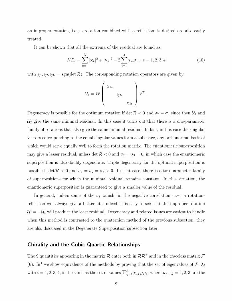
It can be shown that all the extrema of the residual are found as:

NEs =N∑k=1

|xk|2 + |yk|2 − 23∑i=1

χisσi , s = 1, 2, 3, 4 (10)

with χ1sχ2sχ3s = sgn(detR). The corresponding rotation operators are given by

Us =W

χ1s

χ2s

χ3s

VT .Degeneracy is possible for the optimum rotation if detR < 0 and σ2 = σ3 since then U1 and

U2 give the same minimal residual. In this case it turns out that there is a one-parameter

family of rotations that also give the same minimal residual. In fact, in this case the singular

vectors corresponding to the equal singular values form a subspace, any orthonormal basis of

which would serve equally well to form the rotation matrix. The enantiomeric superposition

may give a lesser residual, unless detR < 0 and σ2 = σ3 = 0, in which case the enantiomeric

superposition is also doubly degenerate. Triple degeneracy for the optimal superposition is

possible if detR < 0 and σ1 = σ2 = σ3 > 0. In that case, there is a two-parameter family

of superpositions for which the minimal residual remains constant. In this situation, the

enantiomeric superposition is guaranteed to give a smaller value of the residual.

In general, unless some of the σi vanish, in the negative correlation case, a rotation-

reflection will always give a better fit. Indeed, it is easy to see that the improper rotation

U ′ = −U4 will produce the least residual. Degeneracy and related issues are easiest to handle

when this method is contrasted to the quaternion method of the previous subsection; they

are also discussed in the Degenerate Superposition subsection later.

Chirality and the Cubic-Quartic Relationships

The 9 quantities appearing in the matrix R enter both in RRT and in the traceless matrix F

(6). In1 we show equivalence of the methods by proving that the set of eigenvalues of F , λi

with i = 1, 2, 3, 4, is the same as the set of values∑3

j=1 χ1j√µj, where µj , j = 1, 2, 3 are the

9

eigenvalues of RRT . This is true because the characteristic polynomial of RRT , P3(z) :=∑30 bjz

j, must be the resolvent cubic of P4(λ) :=∑4

0 ajλj, the characteristic polynomial of

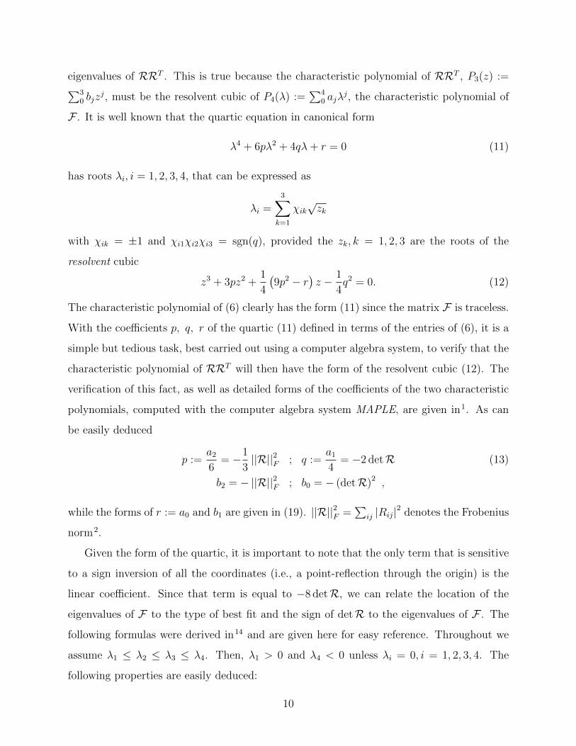
F . It is well known that the quartic equation in canonical form

λ4 + 6pλ2 + 4qλ+ r = 0 (11)

has roots λi, i = 1, 2, 3, 4, that can be expressed as

λi =3∑

k=1

χik√zk

with χik = ±1 and χi1χi2χi3 = sgn(q), provided the zk, k = 1, 2, 3 are the roots of the

resolvent cubic

z3 + 3pz2 +1

4

(9p2 − r

)z − 1

4q2 = 0. (12)

The characteristic polynomial of (6) clearly has the form (11) since the matrix F is traceless.

With the coefficients p, q, r of the quartic (11) defined in terms of the entries of (6), it is a

simple but tedious task, best carried out using a computer algebra system, to verify that the

characteristic polynomial of RRT will then have the form of the resolvent cubic (12). The

verification of this fact, as well as detailed forms of the coefficients of the two characteristic

polynomials, computed with the computer algebra system MAPLE, are given in1. As can

be easily deduced

p :=a2

6= −1

3||R||2F ; q :=

a1

4= −2 detR (13)

b2 = − ||R||2F ; b0 = − (detR)2 ,

while the forms of r := a0 and b1 are given in (19). ||R||2F =∑

ij |Rij|2 denotes the Frobenius

norm2.

Given the form of the quartic, it is important to note that the only term that is sensitive

to a sign inversion of all the coordinates (i.e., a point-reflection through the origin) is the

linear coefficient. Since that term is equal to −8 detR, we can relate the location of the

eigenvalues of F to the type of best fit and the sign of detR to the eigenvalues of F . The

following formulas were derived in14 and are given here for easy reference. Throughout we

assume λ1 ≤ λ2 ≤ λ3 ≤ λ4. Then, λ1 > 0 and λ4 < 0 unless λi = 0, i = 1, 2, 3, 4. The

following properties are easily deduced:

10

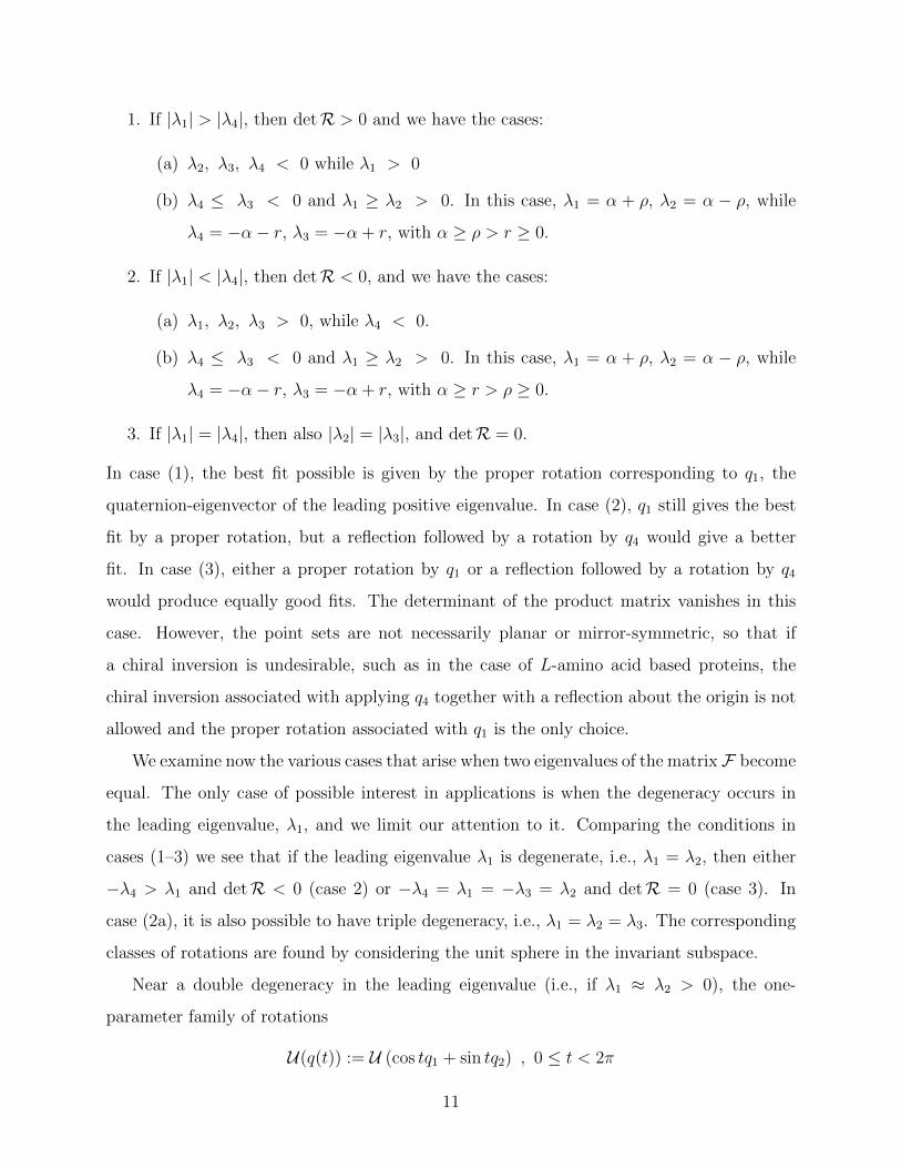
1. If |λ1| > |λ4|, then detR > 0 and we have the cases:

(a) λ2, λ3, λ4 < 0 while λ1 > 0

(b) λ4 ≤ λ3 < 0 and λ1 ≥ λ2 > 0. In this case, λ1 = α + ρ, λ2 = α − ρ, while

λ4 = −α− r, λ3 = −α + r, with α ≥ ρ > r ≥ 0.

2. If |λ1| < |λ4|, then detR < 0, and we have the cases:

(a) λ1, λ2, λ3 > 0, while λ4 < 0.

(b) λ4 ≤ λ3 < 0 and λ1 ≥ λ2 > 0. In this case, λ1 = α + ρ, λ2 = α − ρ, while

λ4 = −α− r, λ3 = −α + r, with α ≥ r > ρ ≥ 0.

3. If |λ1| = |λ4|, then also |λ2| = |λ3|, and detR = 0.

In case (1), the best fit possible is given by the proper rotation corresponding to q1, the

quaternion-eigenvector of the leading positive eigenvalue. In case (2), q1 still gives the best

fit by a proper rotation, but a reflection followed by a rotation by q4 would give a better

fit. In case (3), either a proper rotation by q1 or a reflection followed by a rotation by q4

would produce equally good fits. The determinant of the product matrix vanishes in this

case. However, the point sets are not necessarily planar or mirror-symmetric, so that if

a chiral inversion is undesirable, such as in the case of L-amino acid based proteins, the

chiral inversion associated with applying q4 together with a reflection about the origin is not

allowed and the proper rotation associated with q1 is the only choice.

We examine now the various cases that arise when two eigenvalues of the matrix F become

equal. The only case of possible interest in applications is when the degeneracy occurs in

the leading eigenvalue, λ1, and we limit our attention to it. Comparing the conditions in

cases (1–3) we see that if the leading eigenvalue λ1 is degenerate, i.e., λ1 = λ2, then either

−λ4 > λ1 and detR < 0 (case 2) or −λ4 = λ1 = −λ3 = λ2 and detR = 0 (case 3). In

case (2a), it is also possible to have triple degeneracy, i.e., λ1 = λ2 = λ3. The corresponding

classes of rotations are found by considering the unit sphere in the invariant subspace.

Near a double degeneracy in the leading eigenvalue (i.e., if λ1 ≈ λ2 > 0), the one-

parameter family of rotations

U(q(t)) := U (cos tq1 + sin tq2) , 0 ≤ t < 2π

11

produces near minimal residual for all values of the parameter t. Of course, at the point

of degeneracy, all such rotations produce equal, and minimal, residuals since q(t) is also a

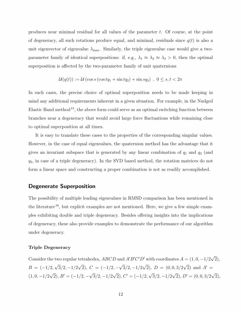
unit eigenvector of eigenvalue λmax. Similarly, the triple eigenvalue case would give a two-

parameter family of identical superpositions: if, e.g., λ1 ≈ λ2 ≈ λ3 > 0, then the optimal

superposition is affected by the two-parameter family of unit quaternions

U(q(t)) := U (cos s (cos tq1 + sin tq2) + sin sq3) , 0 ≤ s, t < 2π

In such cases, the precise choice of optimal superposition needs to be made keeping in

mind any additional requirements inherent in a given situation. For example, in the Nudged

Elastic Band method15, the above form could serve as an optimal switching function between

branches near a degeneracy that would avoid large force fluctuations while remaining close

to optimal superposition at all times.

It is easy to translate these cases to the properties of the corresponding singular values.

However, in the case of equal eigenvalues, the quaternion method has the advantage that it

gives an invariant subspace that is generated by any linear combination of q1 and q2 (and

q3, in case of a triple degeneracy). In the SVD based method, the rotation matrices do not

form a linear space and constructing a proper combination is not as readily accomplished.

Degenerate Superposition

The possibility of multiple leading eigenvalues in RMSD comparison has been mentioned in

the literature16, but explicit examples are not mentioned. Here, we give a few simple exam-

ples exhibiting double and triple degeneracy. Besides offering insights into the implications

of degeneracy, these also provide examples to demonstrate the performance of our algorithm

under degeneracy.

Triple Degeneracy

Consider the two regular tetrahedra, ABCD andA′B′C ′D′ with coordinatesA = (1, 0,−1/2√

2),

B = (−1/2,√

3/2,−1/2√

2), C = (−1/2,−√

3/2,−1/2√

2), D = (0, 0, 3/2√

2) and A′ =

(1, 0,−1/2√

2), B′ = (−1/2,−√

3/2,−1/2√

2), C ′ = (−1/2,√

3/2,−1/2√

2), D′ = (0, 0, 3/2√

2),

12

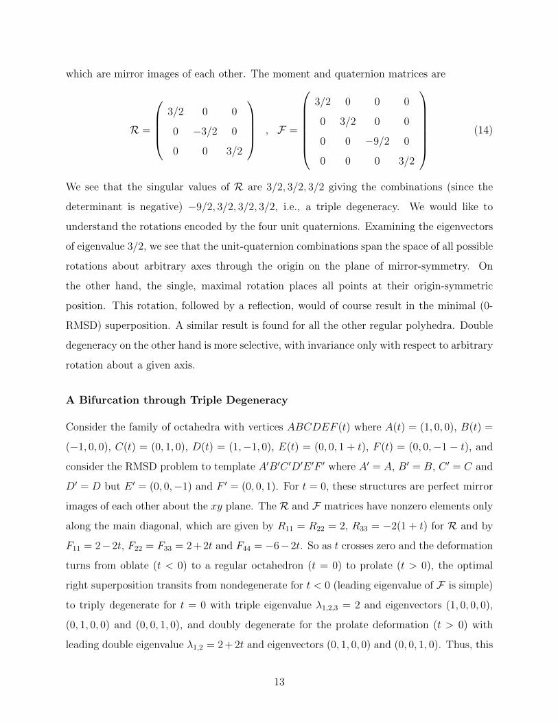
which are mirror images of each other. The moment and quaternion matrices are

R =

3/2 0 0

0 −3/2 0

0 0 3/2

, F =

3/2 0 0 0

0 3/2 0 0

0 0 −9/2 0

0 0 0 3/2

(14)

We see that the singular values of R are 3/2, 3/2, 3/2 giving the combinations (since the

determinant is negative) −9/2, 3/2, 3/2, 3/2, i.e., a triple degeneracy. We would like to

understand the rotations encoded by the four unit quaternions. Examining the eigenvectors

of eigenvalue 3/2, we see that the unit-quaternion combinations span the space of all possible

rotations about arbitrary axes through the origin on the plane of mirror-symmetry. On

the other hand, the single, maximal rotation places all points at their origin-symmetric

position. This rotation, followed by a reflection, would of course result in the minimal (0-

RMSD) superposition. A similar result is found for all the other regular polyhedra. Double

degeneracy on the other hand is more selective, with invariance only with respect to arbitrary

rotation about a given axis.

A Bifurcation through Triple Degeneracy

Consider the family of octahedra with vertices ABCDEF (t) where A(t) = (1, 0, 0), B(t) =

(−1, 0, 0), C(t) = (0, 1, 0), D(t) = (1,−1, 0), E(t) = (0, 0, 1 + t), F (t) = (0, 0,−1 − t), and

consider the RMSD problem to template A′B′C ′D′E ′F ′ where A′ = A, B′ = B, C ′ = C and

D′ = D but E ′ = (0, 0,−1) and F ′ = (0, 0, 1). For t = 0, these structures are perfect mirror

images of each other about the xy plane. The R and F matrices have nonzero elements only

along the main diagonal, which are given by R11 = R22 = 2, R33 = −2(1 + t) for R and by

F11 = 2−2t, F22 = F33 = 2 + 2t and F44 = −6−2t. So as t crosses zero and the deformation

turns from oblate (t < 0) to a regular octahedron (t = 0) to prolate (t > 0), the optimal

right superposition transits from nondegenerate for t < 0 (leading eigenvalue of F is simple)

to triply degenerate for t = 0 with triple eigenvalue λ1,2,3 = 2 and eigenvectors (1, 0, 0, 0),

(0, 1, 0, 0) and (0, 0, 1, 0), and doubly degenerate for the prolate deformation (t > 0) with

leading double eigenvalue λ1,2 = 2 + 2t and eigenvectors (0, 1, 0, 0) and (0, 0, 1, 0). Thus, this

13

corresponds to any quaternion with components (0, cos ζ, sin ζ, 0), i.e., a rotation by angle

θ = π about the Cartesian unit vector (cos ζ, sin ζ, 0) where ζ is an arbitrary parameter.

We see that for oblate deformation there is a unique preferred match which associates

the four vertices in the xy-plane, while the (nearer-placed) vertices along the z-axis remain

mismatched. For the triply degenerate case, the optimal match happens indifferently for

any arbitrary rotation about an arbitrary axis on the xy-plane. For the doubly degenerate

prolate case, the preferred match perfectly aligns the z-axis points while the four vertices on

the xy-plane are antialigned, which is neutral as regards the actual net rotation about the

z-axis.

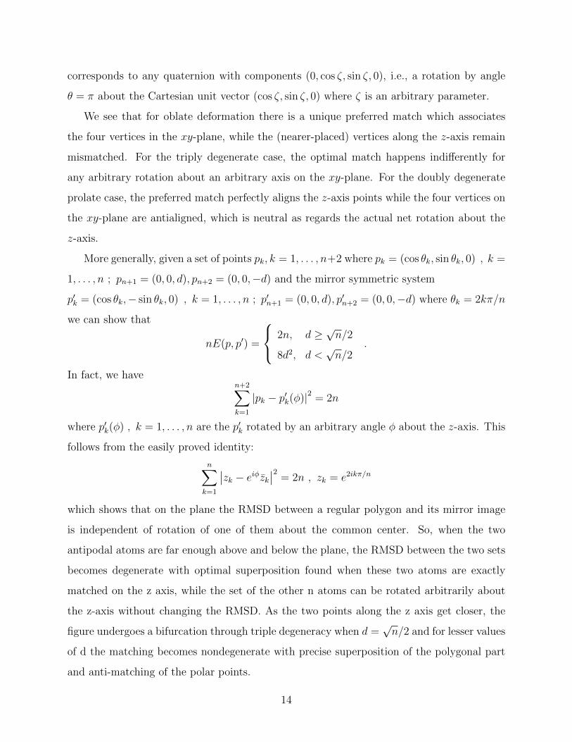
More generally, given a set of points pk, k = 1, . . . , n+2 where pk = (cos θk, sin θk, 0) , k =

1, . . . , n ; pn+1 = (0, 0, d), pn+2 = (0, 0,−d) and the mirror symmetric system

p′k = (cos θk,− sin θk, 0) , k = 1, . . . , n ; p′n+1 = (0, 0, d), p′n+2 = (0, 0,−d) where θk = 2kπ/n

we can show that

nE(p, p′) =

2n, d ≥√n/2

8d2, d <√n/2

.

In fact, we haven+2∑k=1

|pk − p′k(φ)|2 = 2n

where p′k(φ) , k = 1, . . . , n are the p′k rotated by an arbitrary angle φ about the z-axis. This

follows from the easily proved identity:

n∑k=1

∣∣zk − eiφzk∣∣2 = 2n , zk = e2ikπ/n

which shows that on the plane the RMSD between a regular polygon and its mirror image

is independent of rotation of one of them about the common center. So, when the two

antipodal atoms are far enough above and below the plane, the RMSD between the two sets

becomes degenerate with optimal superposition found when these two atoms are exactly

matched on the z axis, while the set of the other n atoms can be rotated arbitrarily about

the z-axis without changing the RMSD. As the two points along the z axis get closer, the

figure undergoes a bifurcation through triple degeneracy when d =√n/2 and for lesser values

of d the matching becomes nondegenerate with precise superposition of the polygonal part

and anti-matching of the polar points.

14

The Coefficients of the Characteristic Polynomial and the Computation

of the Leading Eigenvalue

If it is desired to find all the eigenvalues and eigenvectors of the RMSD matrix, then it

appears that the method of choice would be to apply the QR iteration to the RMSD matrix

F , and the SVD method would be a close competitor. There is no clear conceptual advantage

to either method if one pays attention to the chirality of the singular vector matrices as was

pointed out in11. For most practical applications, we are chiefly interested in the optimal

superposition residual and in some cases on the attendant rotation. As was pointed out by

Theobald8, the leading eigenvalue computation may be performed efficiently by locating the

maximal positive root of the characteristic polynomial of the quaternion matrix F . Here,

the quaternion method is clearly superior, since determining the minimal residual using the

SVD method still requires finding all the singular values. However, it turns out that forming

the characteristic polynomial of the normal equation matrix RRT does offer a substantial

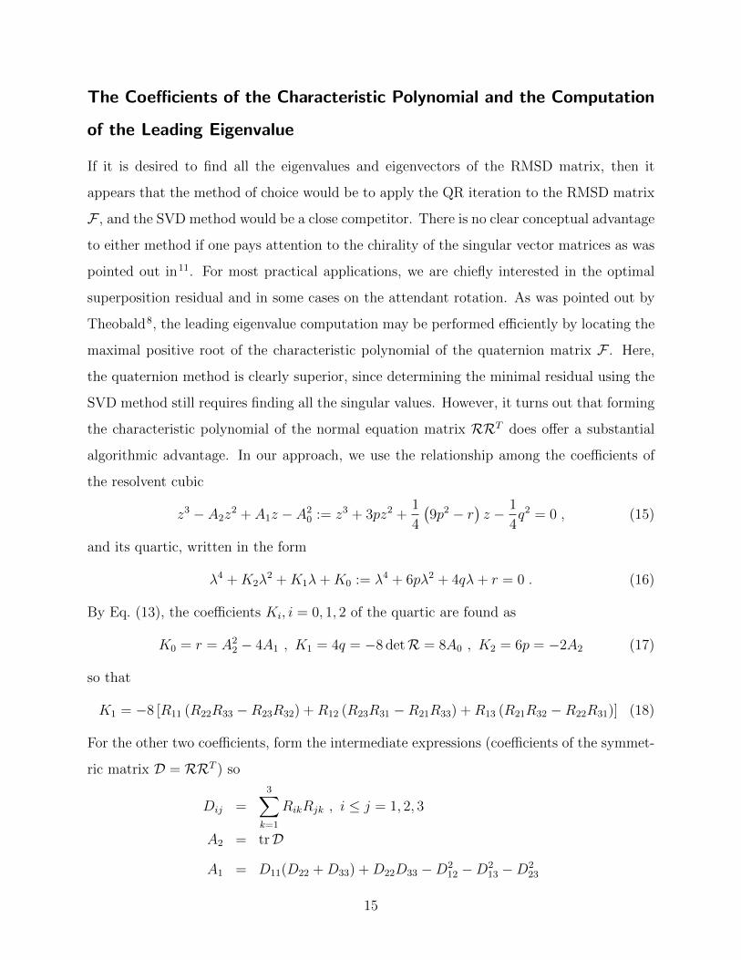
algorithmic advantage. In our approach, we use the relationship among the coefficients of

the resolvent cubic

z3 − A2z2 + A1z − A2

0 := z3 + 3pz2 +1

4

(9p2 − r

)z − 1

4q2 = 0 , (15)

and its quartic, written in the form

λ4 +K2λ2 +K1λ+K0 := λ4 + 6pλ2 + 4qλ+ r = 0 . (16)

By Eq. (13), the coefficients Ki, i = 0, 1, 2 of the quartic are found as

K0 = r = A22 − 4A1 , K1 = 4q = −8 detR = 8A0 , K2 = 6p = −2A2 (17)

so that

K1 = −8 [R11 (R22R33 −R23R32) +R12 (R23R31 −R21R33) +R13 (R21R32 −R22R31)] (18)

For the other two coefficients, form the intermediate expressions (coefficients of the symmet-

ric matrix D = RRT ) so

Dij =3∑

k=1

RikRjk , i ≤ j = 1, 2, 3

A2 = trD

A1 = D11(D22 +D33) +D22D33 −D212 −D2

13 −D223

15

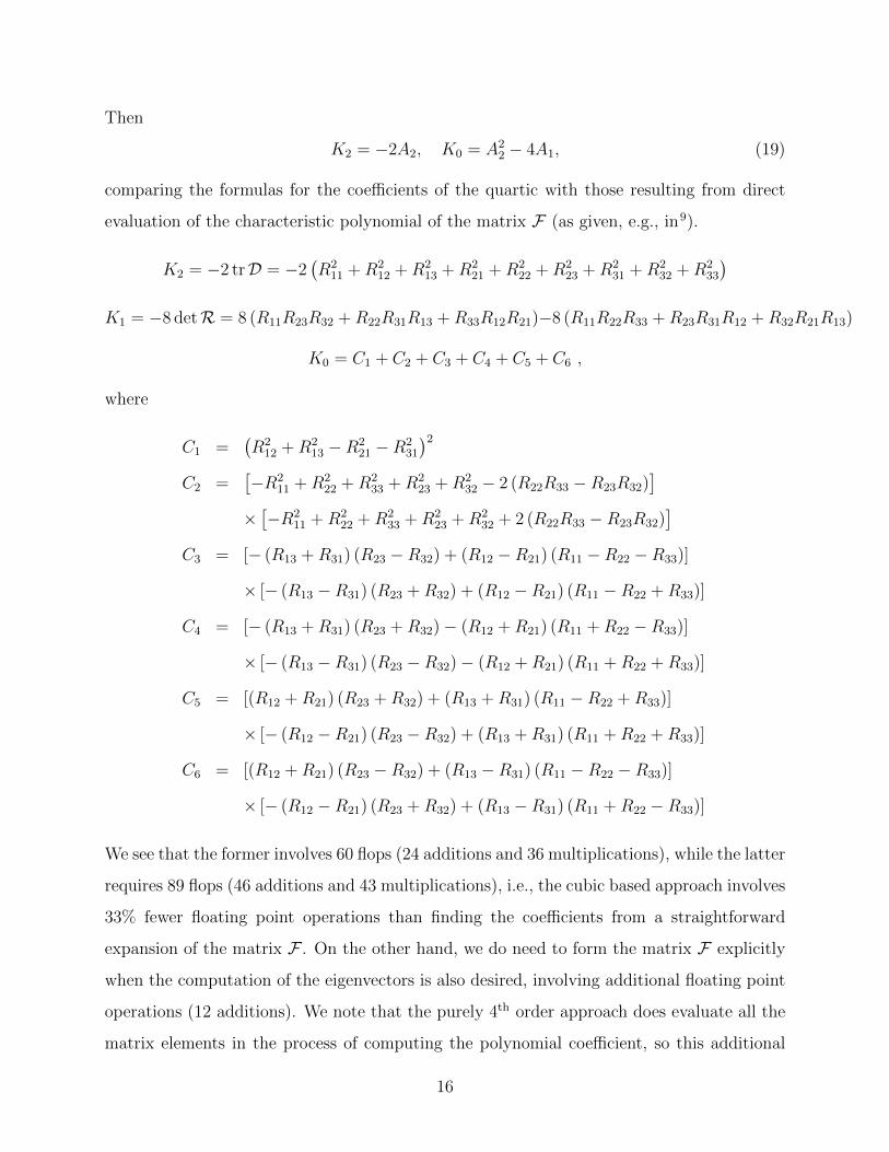
Then

K2 = −2A2, K0 = A22 − 4A1, (19)

comparing the formulas for the coefficients of the quartic with those resulting from direct

evaluation of the characteristic polynomial of the matrix F (as given, e.g., in9).

K2 = −2 trD = −2(R2

11 +R212 +R2

13 +R221 +R2

22 +R223 +R2

31 +R232 +R2

33

)K1 = −8 detR = 8 (R11R23R32 +R22R31R13 +R33R12R21)−8 (R11R22R33 +R23R31R12 +R32R21R13)

K0 = C1 + C2 + C3 + C4 + C5 + C6 ,

where

C1 =(R2

12 +R213 −R2

21 −R231

)2

C2 =[−R2

11 +R222 +R2

33 +R223 +R2

32 − 2 (R22R33 −R23R32)]

×[−R2

11 +R222 +R2

33 +R223 +R2

32 + 2 (R22R33 −R23R32)]

C3 = [− (R13 +R31) (R23 −R32) + (R12 −R21) (R11 −R22 −R33)]

× [− (R13 −R31) (R23 +R32) + (R12 −R21) (R11 −R22 +R33)]

C4 = [− (R13 +R31) (R23 +R32)− (R12 +R21) (R11 +R22 −R33)]

× [− (R13 −R31) (R23 −R32)− (R12 +R21) (R11 +R22 +R33)]

C5 = [(R12 +R21) (R23 +R32) + (R13 +R31) (R11 −R22 +R33)]

× [− (R12 −R21) (R23 −R32) + (R13 +R31) (R11 +R22 +R33)]

C6 = [(R12 +R21) (R23 −R32) + (R13 −R31) (R11 −R22 −R33)]

× [− (R12 −R21) (R23 +R32) + (R13 −R31) (R11 +R22 −R33)]

We see that the former involves 60 flops (24 additions and 36 multiplications), while the latter

requires 89 flops (46 additions and 43 multiplications), i.e., the cubic based approach involves

33% fewer floating point operations than finding the coefficients from a straightforward

expansion of the matrix F . On the other hand, we do need to form the matrix F explicitly

when the computation of the eigenvectors is also desired, involving additional floating point

operations (12 additions). We note that the purely 4th order approach does evaluate all the

matrix elements in the process of computing the polynomial coefficient, so this additional

16

overhead only affects the mixed approach. Nevertheless, even when eigenvectors are required,

the mixed approach is 25% more efficient than the pure quartic approach. So hinging on

the need to compute the optimal rotation matrix in addition to computing the RMSD, the

mixed approach is more efficient in terms of flops required per matrix setup by 25–33%. We

have found that implementation details (discussed at length in Supporting Information A)

are as important for performance.

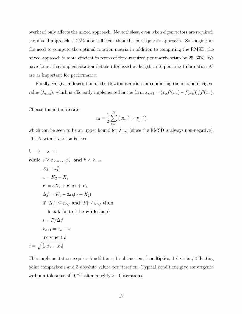
Finally, we give a description of the Newton iteration for computing the maximum eigen-

value (λmax), which is efficiently implemented in the form xn+1 = (xnf′(xn)− f(xn))/f ′(xn):

Choose the initial iterate

x0 =1

2

N∑k=1

(|xk|2 + |yk|2

)which can be seen to be an upper bound for λmax (since the RMSD is always non-negative).

The Newton iteration is then

k = 0; s = 1

while s ≥ εNewton|xk| and k < kmax

X2 = x2k

a = K2 +X2

F = aX2 +K1xk +K0

∆f = K1 + 2xk(a+X2)

if |∆f | ≤ ε∆f and |F | ≤ ε∆f then

break (out of the while loop)

s = F/∆f

xk+1 = xk − s

increment k

e =√

2N|xk − x0|

This implementation requires 5 additions, 1 subtraction, 6 multiplies, 1 division, 3 floating

point comparisons and 3 absolute values per iteration. Typical conditions give convergence

within a tolerance of 10−14 after roughly 5–10 iterations.

17

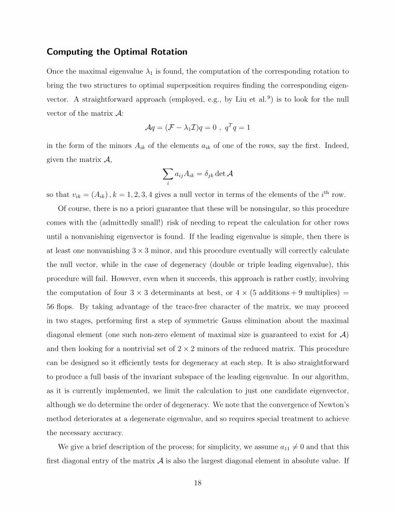
Computing the Optimal Rotation

Once the maximal eigenvalue λ1 is found, the computation of the corresponding rotation to

bring the two structures to optimal superposition requires finding the corresponding eigen-

vector. A straightforward approach (employed, e.g., by Liu et al.9) is to look for the null

vector of the matrix A:

Aq = (F − λ1I)q = 0 , qT q = 1

in the form of the minors Aik of the elements aik of one of the rows, say the first. Indeed,

given the matrix A, ∑i

aijAik = δjk detA

so that vik = (Aik) , k = 1, 2, 3, 4 gives a null vector in terms of the elements of the ith row.

Of course, there is no a priori guarantee that these will be nonsingular, so this procedure

comes with the (admittedly small!) risk of needing to repeat the calculation for other rows

until a nonvanishing eigenvector is found. If the leading eigenvalue is simple, then there is

at least one nonvanishing 3× 3 minor, and this procedure eventually will correctly calculate

the null vector, while in the case of degeneracy (double or triple leading eigenvalue), this

procedure will fail. However, even when it succeeds, this approach is rather costly, involving

the computation of four 3 × 3 determinants at best, or 4 × (5 additions + 9 multiplies) =

56 flops. By taking advantage of the trace-free character of the matrix, we may proceed

in two stages, performing first a step of symmetric Gauss elimination about the maximal

diagonal element (one such non-zero element of maximal size is guaranteed to exist for A)

and then looking for a nontrivial set of 2× 2 minors of the reduced matrix. This procedure

can be designed so it efficiently tests for degeneracy at each step. It is also straightforward

to produce a full basis of the invariant subspace of the leading eigenvalue. In our algorithm,

as it is currently implemented, we limit the calculation to just one candidate eigenvector,

although we do determine the order of degeneracy. We note that the convergence of Newton’s

method deteriorates at a degenerate eigenvalue, and so requires special treatment to achieve

the necessary accuracy.

We give a brief description of the process; for simplicity, we assume a11 6= 0 and that this

first diagonal entry of the matrix A is also the largest diagonal element in absolute value. If

18

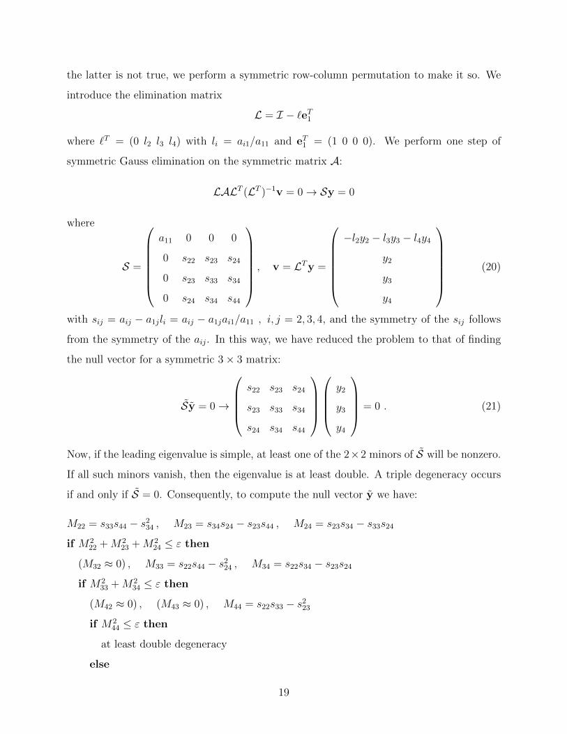
the latter is not true, we perform a symmetric row-column permutation to make it so. We

introduce the elimination matrix

L = I − `eT1

where `T = (0 l2 l3 l4) with li = ai1/a11 and eT1 = (1 0 0 0). We perform one step of

symmetric Gauss elimination on the symmetric matrix A:

LALT (LT )−1v = 0→ Sy = 0

where

S =

a11 0 0 0

0 s22 s23 s24

0 s23 s33 s34

0 s24 s34 s44

, v = LTy =

−l2y2 − l3y3 − l4y4

y2

y3

y4

(20)

with sij = aij − a1jli = aij − a1jai1/a11 , i, j = 2, 3, 4, and the symmetry of the sij follows

from the symmetry of the aij. In this way, we have reduced the problem to that of finding

the null vector for a symmetric 3× 3 matrix:

Sy = 0→

s22 s23 s24

s23 s33 s34

s24 s34 s44

y2

y3

y4

= 0 . (21)

Now, if the leading eigenvalue is simple, at least one of the 2×2 minors of S will be nonzero.

If all such minors vanish, then the eigenvalue is at least double. A triple degeneracy occurs

if and only if S = 0. Consequently, to compute the null vector y we have:

M22 = s33s44 − s234 , M23 = s34s24 − s23s44 , M24 = s23s34 − s33s24

if M222 +M2

23 +M224 ≤ ε then

(M32 ≈ 0) , M33 = s22s44 − s224 , M34 = s22s34 − s23s24

if M233 +M2

34 ≤ ε then

(M42 ≈ 0) , (M43 ≈ 0) , M44 = s22s33 − s223

if M244 ≤ ε then

at least double degeneracy

else

19

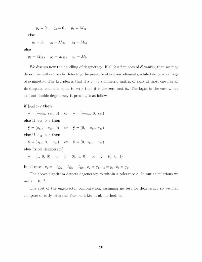
y2 = 0 , y3 = 0 , y4 = M44

else

y2 = 0 , y3 = M33 , y4 = M34

else

y2 = M22 , y3 = M23 , y4 = M24

We discuss now the handling of degeneracy. If all 2× 2 minors of S vanish, then we may

determine null vectors by detecting the presence of nonzero elements, while taking advantage

of symmetry. The key idea is that if a 3 × 3 symmetric matrix of rank at most one has all

its diagonal elements equal to zero, then it is the zero matrix. The logic, in the case where

at least double degeneracy is present, is as follows:

if |s22| > ε then

y = (−s23, s22, 0) or y = (−s24, 0, s22)

else if |s33| > ε then

y = (s33, −s23, 0) or y = (0, −s34, s33)

else if |s44| > ε then

y = (s44, 0, −s24) or y = (0, s44, −s34)

else [triple degeneracy]

y = (1, 0, 0) or y = (0, 1, 0) or y = (0, 0, 1)

In all cases, v1 = −l2y2 − l3y3 − l4y4, v2 = y2, v3 = y3, v4 = y4.

The above algorithm detects degeneracy to within a tolerance ε. In our calculations we

use ε = 10−6.

The cost of the eigenvector computation, assuming no test for degeneracy so we may

compare directly with the Theobald/Liu et al. method, is:

20

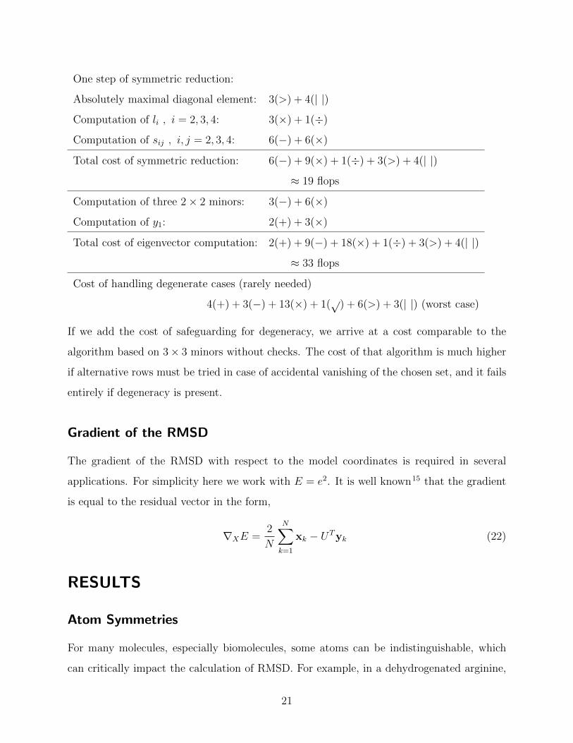
One step of symmetric reduction:

Absolutely maximal diagonal element: 3(>) + 4(| |)

Computation of li , i = 2, 3, 4: 3(×) + 1(÷)

Computation of sij , i, j = 2, 3, 4: 6(−) + 6(×)

Total cost of symmetric reduction: 6(−) + 9(×) + 1(÷) + 3(>) + 4(| |)

≈ 19 flops

Computation of three 2× 2 minors: 3(−) + 6(×)

Computation of y1: 2(+) + 3(×)

Total cost of eigenvector computation: 2(+) + 9(−) + 18(×) + 1(÷) + 3(>) + 4(| |)

≈ 33 flops

Cost of handling degenerate cases (rarely needed)

4(+) + 3(−) + 13(×) + 1(√

) + 6(>) + 3(| |) (worst case)

If we add the cost of safeguarding for degeneracy, we arrive at a cost comparable to the

algorithm based on 3× 3 minors without checks. The cost of that algorithm is much higher

if alternative rows must be tried in case of accidental vanishing of the chosen set, and it fails

entirely if degeneracy is present.

Gradient of the RMSD

The gradient of the RMSD with respect to the model coordinates is required in several

applications. For simplicity here we work with E = e2. It is well known15 that the gradient

is equal to the residual vector in the form,

∇XE =2

N

N∑k=1

xk − UTyk (22)

RESULTS

Atom Symmetries

For many molecules, especially biomolecules, some atoms can be indistinguishable, which

can critically impact the calculation of RMSD. For example, in a dehydrogenated arginine,

21

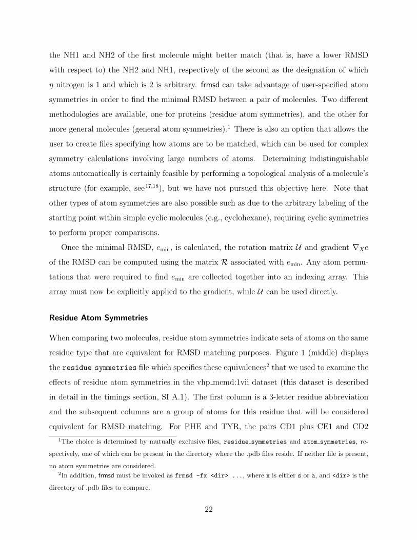
the NH1 and NH2 of the first molecule might better match (that is, have a lower RMSD

with respect to) the NH2 and NH1, respectively of the second as the designation of which

η nitrogen is 1 and which is 2 is arbitrary. frmsd can take advantage of user-specified atom

symmetries in order to find the minimal RMSD between a pair of molecules. Two different

methodologies are available, one for proteins (residue atom symmetries), and the other for

more general molecules (general atom symmetries).1 There is also an option that allows the

user to create files specifying how atoms are to be matched, which can be used for complex

symmetry calculations involving large numbers of atoms. Determining indistinguishable

atoms automatically is certainly feasible by performing a topological analysis of a molecule’s

structure (for example, see17,18), but we have not pursued this objective here. Note that

other types of atom symmetries are also possible such as due to the arbitrary labeling of the

starting point within simple cyclic molecules (e.g., cyclohexane), requiring cyclic symmetries

to perform proper comparisons.

Once the minimal RMSD, emin, is calculated, the rotation matrix U and gradient ∇Xe

of the RMSD can be computed using the matrix R associated with emin. Any atom permu-

tations that were required to find emin are collected together into an indexing array. This

array must now be explicitly applied to the gradient, while U can be used directly.

Residue Atom Symmetries

When comparing two molecules, residue atom symmetries indicate sets of atoms on the same

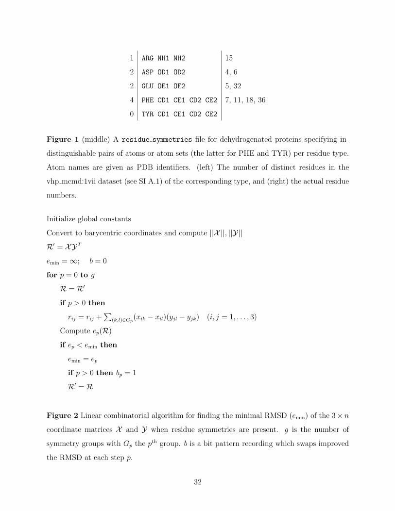
residue type that are equivalent for RMSD matching purposes. Figure 1 (middle) displays

the residue symmetries file which specifies these equivalences2 that we used to examine the

effects of residue atom symmetries in the vhp mcmd:1vii dataset (this dataset is described

in detail in the timings section, SI A.1). The first column is a 3-letter residue abbreviation

and the subsequent columns are a group of atoms for this residue that will be considered

equivalent for RMSD matching. For PHE and TYR, the pairs CD1 plus CE1 and CD2

1The choice is determined by mutually exclusive files, residue symmetries and atom symmetries, re-

spectively, one of which can be present in the directory where the .pdb files reside. If neither file is present,

no atom symmetries are considered.2In addition, frmsd must be invoked as frmsd -fx <dir> ..., where x is either s or a, and <dir> is the

directory of .pdb files to compare.

22

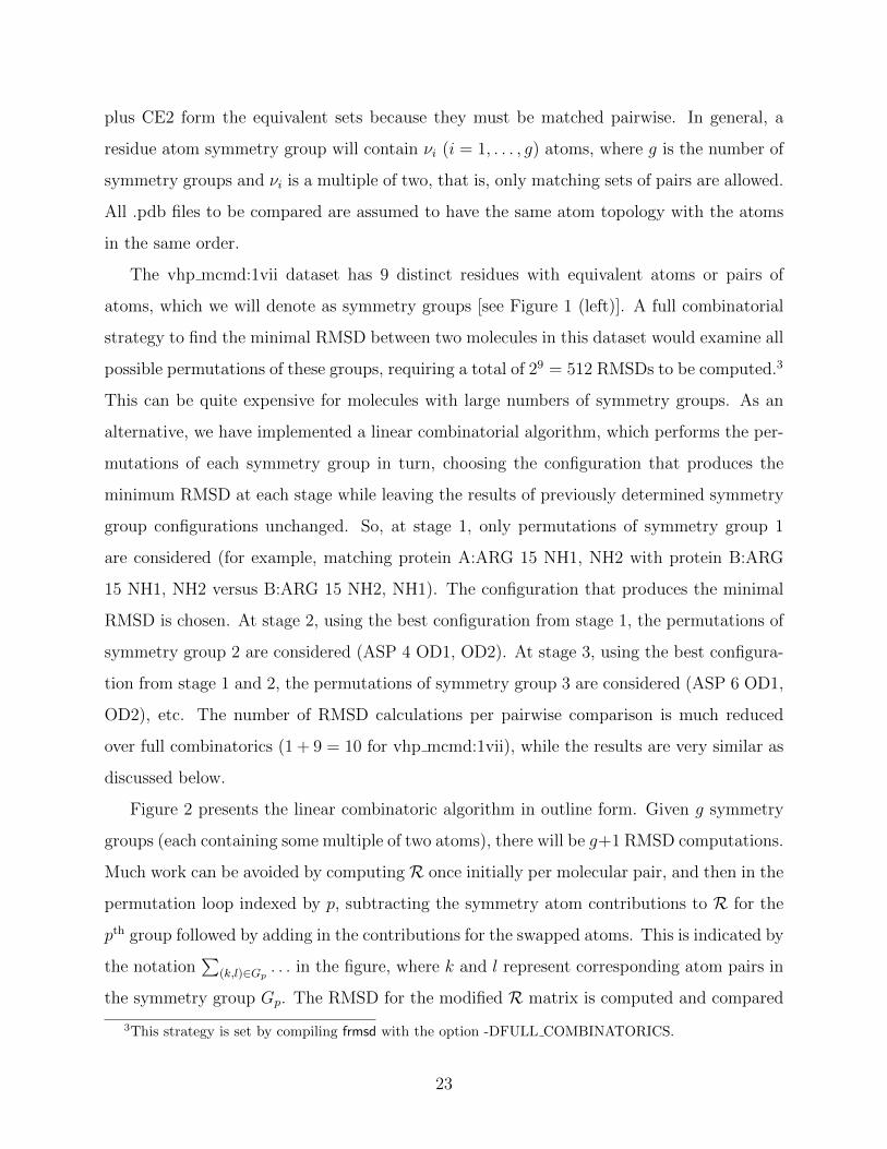
plus CE2 form the equivalent sets because they must be matched pairwise. In general, a

residue atom symmetry group will contain νi (i = 1, . . . , g) atoms, where g is the number of

symmetry groups and νi is a multiple of two, that is, only matching sets of pairs are allowed.

All .pdb files to be compared are assumed to have the same atom topology with the atoms

in the same order.

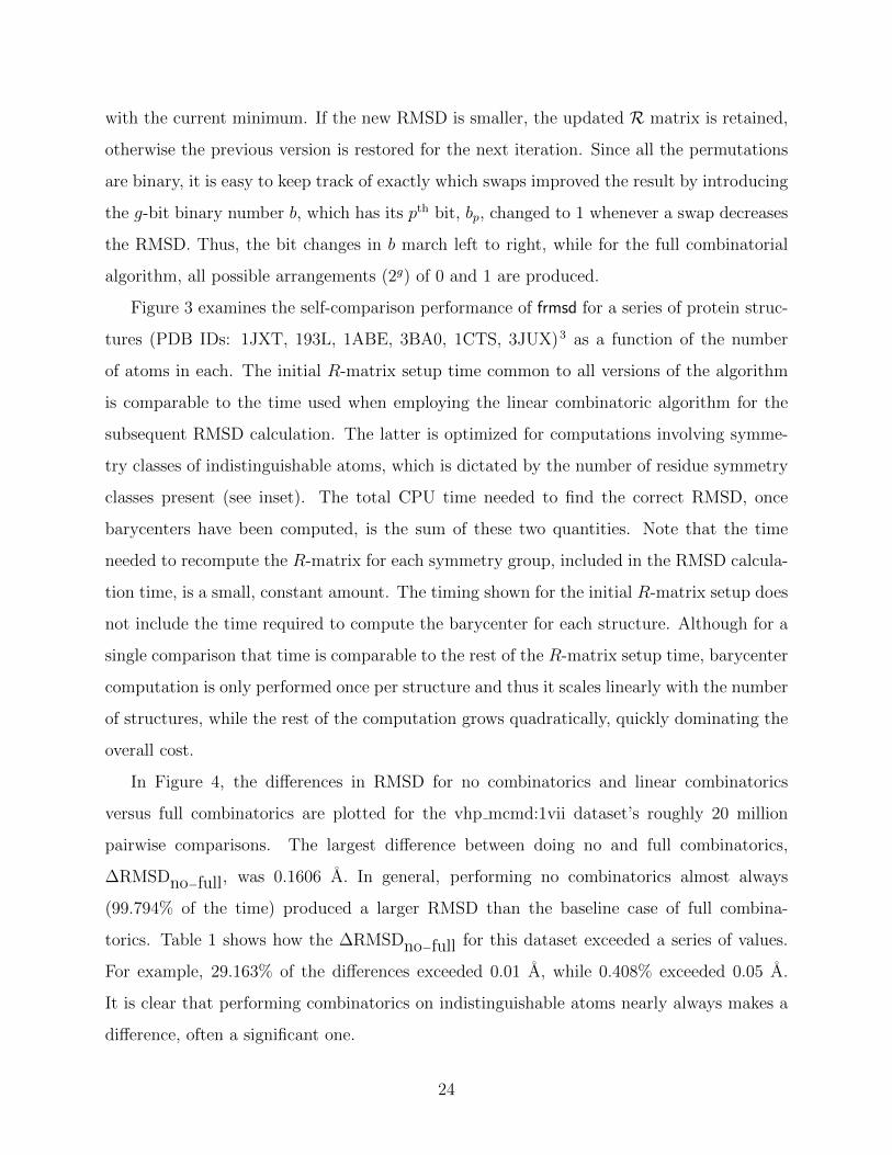
The vhp mcmd:1vii dataset has 9 distinct residues with equivalent atoms or pairs of

atoms, which we will denote as symmetry groups [see Figure 1 (left)]. A full combinatorial

strategy to find the minimal RMSD between two molecules in this dataset would examine all

possible permutations of these groups, requiring a total of 29 = 512 RMSDs to be computed.3

This can be quite expensive for molecules with large numbers of symmetry groups. As an

alternative, we have implemented a linear combinatorial algorithm, which performs the per-

mutations of each symmetry group in turn, choosing the configuration that produces the

minimum RMSD at each stage while leaving the results of previously determined symmetry

group configurations unchanged. So, at stage 1, only permutations of symmetry group 1

are considered (for example, matching protein A:ARG 15 NH1, NH2 with protein B:ARG

15 NH1, NH2 versus B:ARG 15 NH2, NH1). The configuration that produces the minimal

RMSD is chosen. At stage 2, using the best configuration from stage 1, the permutations of

symmetry group 2 are considered (ASP 4 OD1, OD2). At stage 3, using the best configura-

tion from stage 1 and 2, the permutations of symmetry group 3 are considered (ASP 6 OD1,

OD2), etc. The number of RMSD calculations per pairwise comparison is much reduced

over full combinatorics (1 + 9 = 10 for vhp mcmd:1vii), while the results are very similar as

discussed below.

Figure 2 presents the linear combinatoric algorithm in outline form. Given g symmetry

groups (each containing some multiple of two atoms), there will be g+1 RMSD computations.

Much work can be avoided by computing R once initially per molecular pair, and then in the

permutation loop indexed by p, subtracting the symmetry atom contributions to R for the

pth group followed by adding in the contributions for the swapped atoms. This is indicated by

the notation∑

(k,l)∈Gp. . . in the figure, where k and l represent corresponding atom pairs in

the symmetry group Gp. The RMSD for the modified R matrix is computed and compared

3This strategy is set by compiling frmsd with the option -DFULL COMBINATORICS.

23

with the current minimum. If the new RMSD is smaller, the updated R matrix is retained,

otherwise the previous version is restored for the next iteration. Since all the permutations

are binary, it is easy to keep track of exactly which swaps improved the result by introducing

the g-bit binary number b, which has its pth bit, bp, changed to 1 whenever a swap decreases

the RMSD. Thus, the bit changes in b march left to right, while for the full combinatorial

algorithm, all possible arrangements (2g) of 0 and 1 are produced.

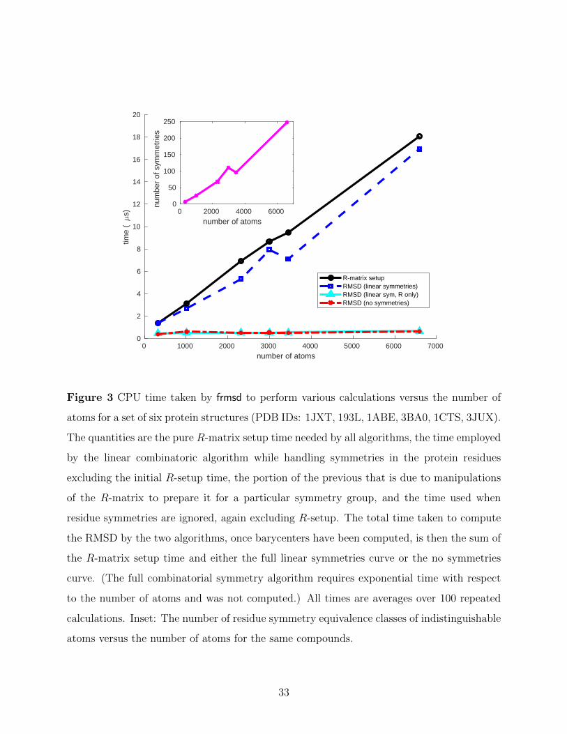
Figure 3 examines the self-comparison performance of frmsd for a series of protein struc-

tures (PDB IDs: 1JXT, 193L, 1ABE, 3BA0, 1CTS, 3JUX)3 as a function of the number

of atoms in each. The initial R-matrix setup time common to all versions of the algorithm

is comparable to the time used when employing the linear combinatoric algorithm for the

subsequent RMSD calculation. The latter is optimized for computations involving symme-

try classes of indistinguishable atoms, which is dictated by the number of residue symmetry

classes present (see inset). The total CPU time needed to find the correct RMSD, once

barycenters have been computed, is the sum of these two quantities. Note that the time

needed to recompute the R-matrix for each symmetry group, included in the RMSD calcula-

tion time, is a small, constant amount. The timing shown for the initial R-matrix setup does

not include the time required to compute the barycenter for each structure. Although for a

single comparison that time is comparable to the rest of the R-matrix setup time, barycenter

computation is only performed once per structure and thus it scales linearly with the number

of structures, while the rest of the computation grows quadratically, quickly dominating the

overall cost.

In Figure 4, the differences in RMSD for no combinatorics and linear combinatorics

versus full combinatorics are plotted for the vhp mcmd:1vii dataset’s roughly 20 million

pairwise comparisons. The largest difference between doing no and full combinatorics,

∆RMSDno−full, was 0.1606 A. In general, performing no combinatorics almost always

(99.794% of the time) produced a larger RMSD than the baseline case of full combina-

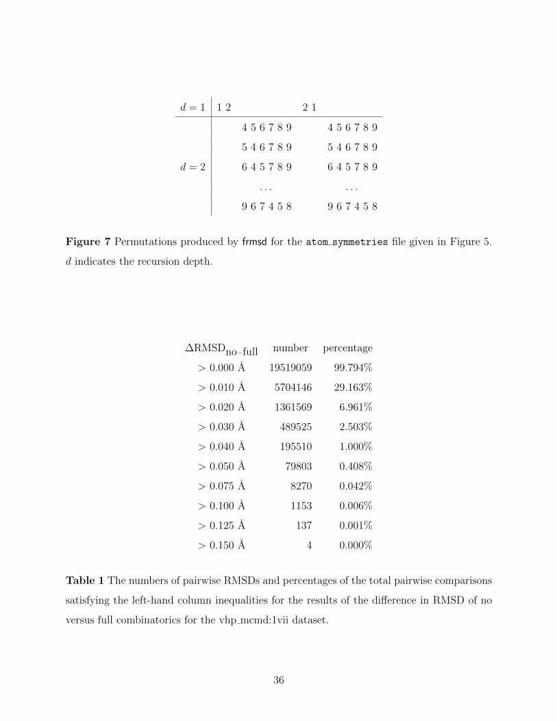
torics. Table 1 shows how the ∆RMSDno−full for this dataset exceeded a series of values.

For example, 29.163% of the differences exceeded 0.01 A, while 0.408% exceeded 0.05 A.

It is clear that performing combinatorics on indistinguishable atoms nearly always makes a

difference, often a significant one.

24

Examining Figure 4 once again, the differences in RMSD between doing linear and full

combinatorics is seen to be small. Only 0.254% of the pairwise comparisons differ at all. The

largest difference is 0.0026 A, corresponding to two configurations that differ in 4 residue atom

symmetry groups. However, the actual RMSD is quite large (10.979 Afor full combinatorics),

so there is quite a bit of play in the atom orientations. For molecules whose RMSD ≤ 1.5 A,

the greatest difference is 5 · 10−6 A, corresponding to a difference of a single residue atom

symmetry group. Only 0.022% of the pairwise comparisons of molecules with RMSD ≤

1.5 Adiffer between the results produced by linear and full combinatorics.

General Atom Symmetries

In addition to residue atom symmetries, frmsd has the capability to deal with more general

atom symmetries if the file atom symmetries is present. Each line defines a set of equivalent

atoms.4 See Figure 5 for an example of such a file. frmsd performs all possible permutations of

the atoms in these sets, returning the permutation with the minimal RMSD. This is done via

a recursive procedure, where each invocation cycles iteratively through all the permutations

of one of the sets. The iterative permutation algorithm19 swaps two indices per permutation

produced, making it possible to efficiently modify the R matrix from its previous value and

then compute a new RMSD. The permutation sets are ordered from smallest to largest in

order to minimize the number of recursive calls.

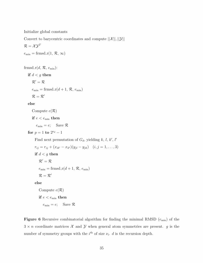
Figure 6 provides a schematic of the recursive algorithm. RMSDs are only computed at

the deepest recursion depth, that is, when d = g, where g is the number of general atom

symmetry groups. At each level d, the iterative permutation algorithm is executed, allowing

R to be modified in the same manner as in the linear combinatorial residue symmetry

algorithm except that now all possible permutations of the general atom symmetry group

corresponding to this depth are performed. Upon completion of the level d permutation

sequence, the procedure returns to the previous level and the R matrix being used there is

restored so that it can be properly updated on the next iteration at that level. As before,

whenever an RMSD smaller than the current emin is computed, it and the corresponding R

are saved as well as a record of the appropriate permutation. An example of this algorithm

4These are referred to by number, with the first atom listed in the .pdb file being number one.

25

in action is shown in Figure 7, which displays the permutations produced for the example

atom symmetries file of Figure 5.

An application where general atom symmetries are important is within a quantum me-

chanical (QM) chemical reaction system in which the RMSD is used as a metric for an

interpolation scheme on a non-uniform multidimensional grid of QM potential energy and

atomic force data.20,21 Here, the molecular configurations all have the same components (so

many carbon atoms, so many hydrogens, etc.), but may be organized (bonded) in different

ways, so it is necessary to group nuclei of the same type and permute them in order find the

distance to the closest reference configuration on the grid.

Graph Symmetry in Polymers

When the molecule is composed of identical subunits in an arrangement with a symmetric

graph, then alternative equivalent alignments may be possible, leading to potentially lower

RMSD. The requirement for this to occur is that the reindexed molecular graph is equivalent

to the original. We demonstrate this on a set of macrocyclic compounds 1P2, AAS, ACX,

BIX, BPH, CD4, CRP, HAX, KCR, MST, RH9, SWI and TET (shown in Fig. SI1 colored to

highlight identical building blocks for each). All the above compounds, listed alphabetically

by short name, with source and full compound name are shown in Table SI7. Table SI8

displays each compound’s number of possible alignments, symmetry type, and the minimum

and maximum RMSD computed over all the alignments as well as the given value if no

symmetries are taken into account.

Here, ACX, MST and TET are hexamers, while BIX, CD4, CRP and KCR are trimers,

and 1P2, AAS, BPH, HAX, RH9 and SWI are dimers. Of these, MST, TET, BIX, CD4

and CRP are composed of subunits with palindromic symmetry. More precisely, the graphs

of MST and TET have tetrahedral symmetry, so that 24 distinct alignments are possible,

while ACX has cyclic symmetry of order 6. All the dimers have cyclic symmetry of order

two. Among the trimers, KCR has cyclic symmetry of order 3, while the others (BIX, CD4,

CRP) have full dihedral symmetry of order 3, and may be aligned “upside-down”, giving a

total of 6 possible alignments. They are reproduced from Coutsias, Lexa et al.22. Invariably,

we found that a lower RMSD was possible for some alignment other than the original, and

26

in a few cases a much lower RMSD was found. This is of course expected, as including all

alternative alignments effectively multiplies the ensemble size by a factor equal to the order

of symmetry of a given compound.

Finding equivalent re-indexings of a molecule as required for a symmetry-based match-

ing can be tedious23,24. The SMARTS25 pattern-matching scheme can be useful here, but

performance seems to vary across implementations26,27.

DISCUSSION

We have developed a fast, robust numerical algorithm to compute the RMSD between a pair

of topologically similar molecular conformations, paying attention to the important role that

various types of symmetry play. We have implemented our algorithm in C under the name

frmsd (for fast RMSD), which we have made publicly available under an open source BSD

license.

frmsd takes advantage of the algebraic equivalence between the characteristic polynomials

of the matrices produced by the quaternion and SVD approaches for directly computing the

RMSD, respectively: a 4 × 4 symmetric, traceless matrix versus a 3× 3 symmetric matrix.

The former quartic polynomial is used in the algorithm qrmsd9, while the latter cubic, the

resolvent cubic of the quartic polynomial, is used by frmsd. Using the SVD formulation

produces very compact forms of the matrix coefficients, while the Newton iteration for com-

puting the maximal eigenvalue is written in such a way so as to require a minimal number of

operations. Symmetric maximal pivoting of the 3×3 matrix allows all structural degenerate

conditions to be discovered, always producing a result no matter what geometric symmetries

are possessed by the molecular configuration.

Along with algorithmic speedups in which the number of flops is minimized, frmsd has

also been optimized in a number of ways (see Supporting Information A) to take advantage

of modern computer CPU architecture. The most important of these optimizations has been

to significantly reduce memory accesses as these operations, especially in deeply nested inner

loops, can significantly affect the performance of a code. frmsd has also been streamlined

to efficiently handle large numbers of RMSD comparisons at a time, such as comparing all

27

molecules defined in a set of PDB coordinate files with either each other or just the first.

This begins by shifting all the molecules under consideration to barycentric coordinates

before computing the optimal rotations.

In addition, atom alignment symmetry, in which the best match for atoms in the same

symmetry class (defined by simple user supplied files) is considered. Atoms in the same

equivalence class are generally numbered in an arbitrary manner (for example, OD1 and

OD2, using PDB notation, in an aspartic acid residue), so simple RMSD matching may not

produce the correct (minimal) RMSD (here, matching the two OD1s with each other and the

two OD2s with each other; one needs to consider matching each OD1 with the other OD2

as well). This problem is very general and can involve more complicated symmetries, such

as paired symmetries (matching CD1 plus CE1 versus CD2 plus CE2 in a phenylalanine or

tyrosine) and cyclic symmetries (the carbon backbone in a cyclohexane ring in which the

choice of the first carbon and the direction of ring traversal are completely arbitrary), etc.

For protein comparisons, frmsd has the capability to deal with the combinatorial explosion

associated with the presence of several symmetries, using an efficient linear combinatoric

search, which is nearly as good as a full combinatoric examination, for the protein residues.

For more general symmetries in which the user specifies sets of indistinguishable atoms,

full combinatorics are applied. In either case, matrix recalculation only involves transposed

atoms, thus minimizing the number of operations that need to be done or redone.

frmsd can compute RMSDs, and produce rotation quaternions and rotation matrices as

well as RMSD gradients. It can also apply the rotations discovered and generate the best

superpositions of one molecule onto a set of conformers, or a set of conformers onto one

molecule. Finally, atoms can be filtered in various ways, so that RMSDs can be performed

only on heavy atoms, protein backbone atoms (N, CA [Cα], C), and CA atoms alone, as

well as all atoms with or without symmetries, or on an arbitrary sublist.

We therefore introduce a general purpose RMSD calculator that exploits symmetry in

multiple ways. A typical application of such a tool is to use the computed RMSDs as a

means of clustering conformers. Included in the distribution is a simple clustering program,

based on frmsd, which performs the following algorithm on a list of structures. The first

structure in the list is taken to be the center of a cluster. All structures whose mutual

28

RMSD with this structure is less than some user-defined threshold are taken to be members

of the cluster, and so are removed from further consideration as possible cluster centers.

The next available structure in the list is then taken to be the center of a new cluster and

the mutual RMSDs with this structure are computed over all structures later in the list.

This process repeats until no more unclustered structures are left. Note that structures

may be members of more than one cluster, which allows the bias of the original ordering to

be ameliorated. An additional criterion, such as energy, may be used to create a natural

ordering before clustering begins.

CONCLUSIONS

We present a highly efficient and robust algorithm for calculating the RMSD that can handle

degeneracy and is optimized for performing alternative comparisons to account for indistin-

guishable atom subgroups. We also give explicit examples of structures with degenerate

superpositions. We exploit the equivalence1 of the quaternion-based formula to the widely

used formula derived by Kabsch4 to elucidate issues related to chirality and degeneracy, and

to arrive at a formulation with minimal algebraic operations as compared to previous im-

plementations. Source code for the software, with tools to perform clustering and multiple

comparisons, are provided.

ACKNOWLEDGMENTS

The authors thank the NIGMS for support (GM090205). Computations were performed at

the Center for Advanced Research Computing, University of New Mexico. EAC acknowl-

edges support from the Laufer Center for Physical and Quantitative Biology at Stony Brook

University. The authors thank Dan Sindhikara for pointing out reference26.

((Additional Supporting Information may be found in the online version of this article.))

29

References

1. E. A. Coutsias, C. Seok, and K. A. Dill, Journal of Computational Chemistry 25, 1849

(2004).

2. R. A. Horn and C. R. Johnson, Matrix Analysis (Cambridge Univ. Press, 1985).

3. G. R. Kneller, J. Comput. Chem. 32, 183 (2011).

4. W. Kabsch, Acta Cryst. A32, 922 (1976).

5. J. L. Tietze, J Astronaut Sci 30, 171 (1982).

6. S. K. Kearsley, Acta Cryst. A45, 208 (1989).

7. G. R. Kneller, Mol Simulat 7, 113 (1991), ISSN 0892-7022.

8. D. L. Theobald, Acta Cryst. A61, 478 (2005).

9. P. Liu, D. K. Agrafiotis, and D. L. Theobald, Journal of Computational Chemistry 31,

1561 (2010).

10. P. Liu, D. K. Agrafiotis, and D. L. Theobald, Journal of Computational Chemistry 32,

185 (2011), ISSN 1096-987X, URL http://dx.doi.org/10.1002/jcc.21606.

11. E. A. Coutsias, C. Seok, and K. A. Dill, Journal of Computational Chemistry 26, 1663

(2005).

12. W. Kabsch, Acta Cryst. A34, 827 (1978).

13. P. H. Schoneman, Psychometrika 31(1), 1 (1966).

14. E. A. Coutsias, C. Seok, M. P. Jacobson, and K. A. Dill, 25, 510 (2004).

15. J. W. Chu, B. L. Trout, and B. R. Brooks, J. Chem. Phys. 119, 12708 (2003).

16. R. Diamond, Acta Cryst. A46, 423 (1990).

17. S. N. Pollock, E. A. Coutsias, M. J. Wester, and T. I. Oprea, Journal of Chemical

Information and Modeling 48, 1304 (2008).

30

18. M. J. Wester, S. N. Pollock, E. A. Coutsias, T. K. Allu, S. Muresan, and T. I. Oprea,

Journal of Chemical Information and Modeling 48, 1311 (2008).

19. P. P. Fuchs, Scalable Permutations: A Permutation of Agreeable Ideas, http://www.

quickperm.org/ (2013), [Online; accessed: January 22, 2013].

20. M. R. Salazar, private communication (2013).

21. M. R. Salazar, private communication (2013).

22. E. A. Coutsias, K. W. Lexa, M. J. Wester, S. N. Pollock, and M. P. Jacobson, Journal

of Chemical Theory and Computation 12, 4674 (2016).

23. J. W. Raymond, E. J. Gardiner, and P. Willett, The Computer Journal 45, 631 (2002).

24. H.-C. Ehrlich and M. Rarey, WIREs Computational Molecular Science 1, 68 (2011).

25. SMARTS Theory Manual, Daylight Chemical Information Systems, Santa Fe, New Mex-

ico (2008), http://www.daylight.com/dayhtml/doc/theory/theory.smarts.html.

26. P. P. Shenkin, S. Davies, and J. Shelley, MMSYM utility, Schrodinger, LLC Release

2018-3 (2018).

27. G. Landrum, Rdkit: Open-source cheminformatics, URL http://www.rdkit.org.

31

1 ARG NH1 NH2 15

2 ASP OD1 OD2 4, 6

2 GLU OE1 OE2 5, 32

4 PHE CD1 CE1 CD2 CE2 7, 11, 18, 36

0 TYR CD1 CE1 CD2 CE2

Figure 1 (middle) A residue symmetries file for dehydrogenated proteins specifying in-

distinguishable pairs of atoms or atom sets (the latter for PHE and TYR) per residue type.

Atom names are given as PDB identifiers. (left) The number of distinct residues in the

vhp mcmd:1vii dataset (see SI A.1) of the corresponding type, and (right) the actual residue

numbers.

Initialize global constants

Convert to barycentric coordinates and compute ||X ||, ||Y||

R′ = XYT

emin =∞; b = 0

for p = 0 to g

R = R′

if p > 0 then

rij = rij +∑

(k,l)∈Gp(xik − xil)(yjl − yjk) (i, j = 1, . . . , 3)

Compute ep(R)

if ep < emin then

emin = ep

if p > 0 then bp = 1

R′ = R

Figure 2 Linear combinatorial algorithm for finding the minimal RMSD (emin) of the 3× n

coordinate matrices X and Y when residue symmetries are present. g is the number of

symmetry groups with Gp the pth group. b is a bit pattern recording which swaps improved

the RMSD at each step p.

32

0 1000 2000 3000 4000 5000 6000 7000

number of atoms

0

2

4

6

8

10

12

14

16

18

20

time

(s)

R-matrix setupRMSD (linear symmetries)RMSD (linear sym, R only)RMSD (no symmetries)

0 2000 4000 6000

number of atoms

0

50

100

150

200

250

num

ber

of s

ymm

etrie

s

Figure 3 CPU time taken by frmsd to perform various calculations versus the number of

atoms for a set of six protein structures (PDB IDs: 1JXT, 193L, 1ABE, 3BA0, 1CTS, 3JUX).

The quantities are the pure R-matrix setup time needed by all algorithms, the time employed

by the linear combinatoric algorithm while handling symmetries in the protein residues

excluding the initial R-setup time, the portion of the previous that is due to manipulations

of the R-matrix to prepare it for a particular symmetry group, and the time used when

residue symmetries are ignored, again excluding R-setup. The total time taken to compute

the RMSD by the two algorithms, once barycenters have been computed, is then the sum of

the R-matrix setup time and either the full linear symmetries curve or the no symmetries

curve. (The full combinatorial symmetry algorithm requires exponential time with respect

to the number of atoms and was not computed.) All times are averages over 100 repeated

calculations. Inset: The number of residue symmetry equivalence classes of indistinguishable

atoms versus the number of atoms for the same compounds.

33

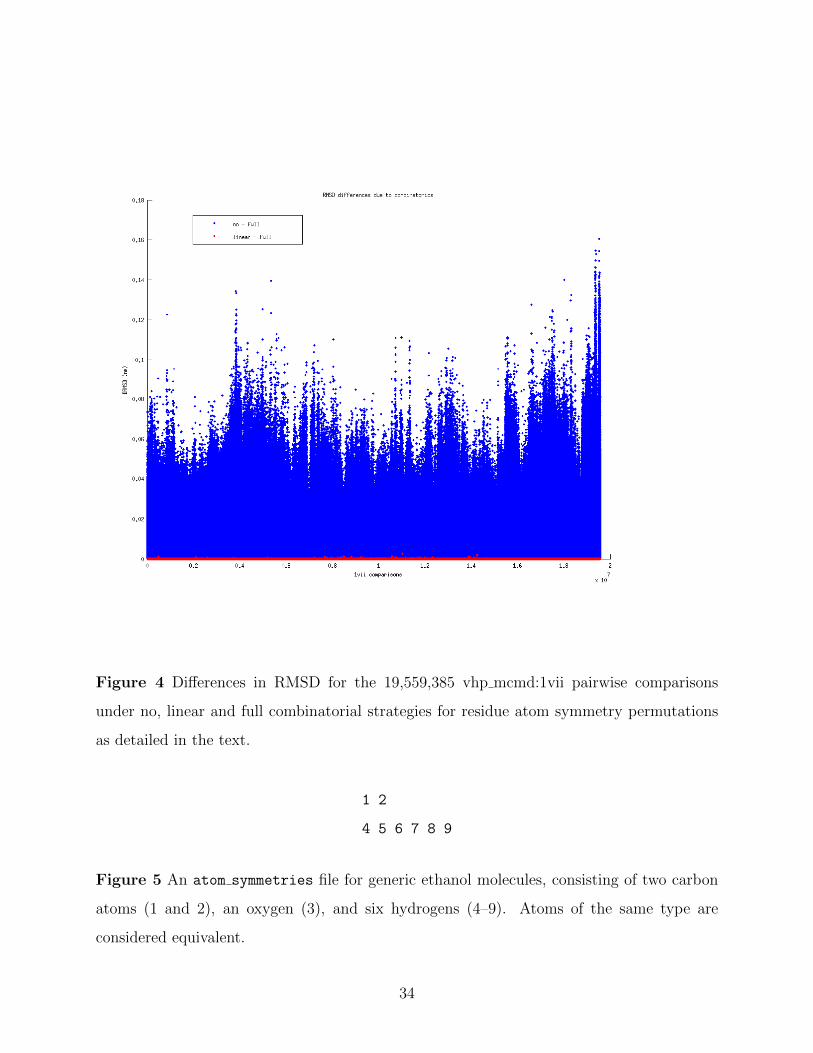
Figure 4 Differences in RMSD for the 19,559,385 vhp mcmd:1vii pairwise comparisons

under no, linear and full combinatorial strategies for residue atom symmetry permutations

as detailed in the text.

1 2

4 5 6 7 8 9

Figure 5 An atom symmetries file for generic ethanol molecules, consisting of two carbon

atoms (1 and 2), an oxygen (3), and six hydrogens (4–9). Atoms of the same type are

considered equivalent.

34

Initialize global constants

Convert to barycentric coordinates and compute ||X ||, ||Y||

R = XYT

emin = frmsd r(1, R, ∞)

frmsd r(d, R, emin):

if d < g then

R′ = R

emin = frmsd r(d+ 1, R, emin)

R = R′

else

Compute e(R)

if e < emin then

emin = e; Save R

for p = 1 to 2νd − 1

Find next permutation of Gd, yielding k, l, k′, l′

rij = rij + (xik′ − xil′)(yjl − yjk) (i, j = 1, . . . , 3)

if d < g then

R′ = R

emin = frmsd r(d+ 1, R, emin)

R = R′

else

Compute e(R)

if e < emin then

emin = e; Save R

Figure 6 Recursive combinatorial algorithm for finding the minimal RMSD (emin) of the

3 × n coordinate matrices X and Y when general atom symmetries are present. g is the

number of symmetry groups with the ith of size νi. d is the recursion depth.

35

d = 1 1 2 2 1

4 5 6 7 8 9 4 5 6 7 8 9

5 4 6 7 8 9 5 4 6 7 8 9

d = 2 6 4 5 7 8 9 6 4 5 7 8 9

. . . . . .

9 6 7 4 5 8 9 6 7 4 5 8

Figure 7 Permutations produced by frmsd for the atom symmetries file given in Figure 5.

d indicates the recursion depth.

∆RMSDno−full number percentage

> 0.000 A 19519059 99.794%

> 0.010 A 5704146 29.163%

> 0.020 A 1361569 6.961%

> 0.030 A 489525 2.503%

> 0.040 A 195510 1.000%

> 0.050 A 79803 0.408%

> 0.075 A 8270 0.042%

> 0.100 A 1153 0.006%

> 0.125 A 137 0.001%

> 0.150 A 4 0.000%

Table 1 The numbers of pairwise RMSDs and percentages of the total pairwise comparisons

satisfying the left-hand column inequalities for the results of the difference in RMSD of no

versus full combinatorics for the vhp mcmd:1vii dataset.

36