RiverFLO-2D Equations Methods 09-30-09

RiverFLO-2D Model RiverFLO-2D Model Governing Equations Governing Equations

and Numerical Methodand Numerical Method

Reinaldo GarciaReinaldo Garcia

FLO-2D Software, Inc.FLO-2D Software, Inc.

September, 2009September, 2009

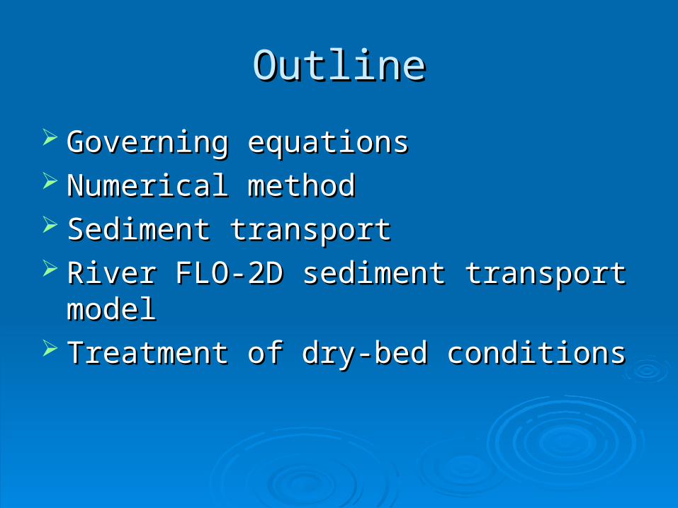
OutlineOutline

Governing equations Governing equations Numerical methodNumerical method Sediment transportSediment transport River FLO-2D sediment transport modelRiver FLO-2D sediment transport model Treatment of dry-bed conditionsTreatment of dry-bed conditions

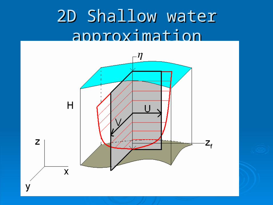
2D Shallow water approximation2D Shallow water approximation

2D Shallow water equations2D Shallow water equations

SWE. Friction termsSWE. Friction terms

Manning’s equationManning’s equation

Allows for other internal friction formulations for Allows for other internal friction formulations for ττbxbx and and ττbyby

Sediment transport model for Sediment transport model for alluvial riversalluvial rivers

Sediment continuity equationSediment continuity equation

Sediment loadSediment load

Sediment transport modelSediment transport model

Meyer-Peter & Muller: Meyer-Peter & Muller:

Sediment transportSediment transport

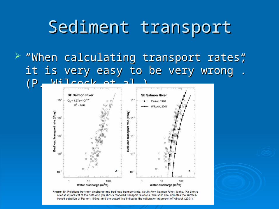
Bed load, suspended load, wash load.Bed load, suspended load, wash load. Substrate vs surface based transport.Substrate vs surface based transport. Sediment transport formulas for substrate sediment.Sediment transport formulas for substrate sediment. ““The main source of uncertainty in calculated The main source of uncertainty in calculated

transport rates arises from uncertainty in the input transport rates arises from uncertainty in the input values of grain size, boundary stress, and hydraulic values of grain size, boundary stress, and hydraulic roughness.”roughness.”

““Too often, the transport formula is blamed for poor Too often, the transport formula is blamed for poor results when the real culprit is poor input.” Wilcock results when the real culprit is poor input.” Wilcock et al.et al.

Sediment transportSediment transport

““When calculating transport rates, it is very easy When calculating transport rates, it is very easy to be very wrong”. (P. Wilcock et al.)to be very wrong”. (P. Wilcock et al.)


Required data: Required data: Substrate sediment D50 (Also D90 for Van Substrate sediment D50 (Also D90 for Van

Rijn formula)Rijn formula) Sediment specific gravitySediment specific gravity Bed porosityBed porosity Inflow boundary conditions for sediment Inflow boundary conditions for sediment

transport assume equilibrium, i.e. Inflow transport assume equilibrium, i.e. Inflow QQss is determined from transport formula. is determined from transport formula.

If this was not enough…If this was not enough…

“…“…by making the computations easier, by making the computations easier, BAGS and similar software makes it possible BAGS and similar software makes it possible to produce inaccurate estimates (even wildly to produce inaccurate estimates (even wildly inaccurate estimates) very quickly and in inaccurate estimates) very quickly and in great abundance.”, Wilcock et al.great abundance.”, Wilcock et al.

Pitlick, John; Cui, Yantao; Wilcock, Peter. 2009. Manual for computing Pitlick, John; Cui, Yantao; Wilcock, Peter. 2009. Manual for computing bed load transport using BAGS (Bedload Assessment for Gravel-bed bed load transport using BAGS (Bedload Assessment for Gravel-bed Streams) Software. Gen. Tech. Rep. RMRS-GTR-223. Fort Collins, CO: Streams) Software. Gen. Tech. Rep. RMRS-GTR-223. Fort Collins, CO: U.S. Department of Agriculture, Forest Service, Rocky Mountain U.S. Department of Agriculture, Forest Service, Rocky Mountain Research Station. 45 p.Research Station. 45 p.

http://www.stream.fs.fed.us/publications/software.html.http://www.stream.fs.fed.us/publications/software.html.


Several sediment transport formulas: Several sediment transport formulas: 1: Meyer-Peter & Muller (1948), 1: Meyer-Peter & Muller (1948), 2: Karim-Kennedy (1998),2: Karim-Kennedy (1998), 3: Ackers-White (1975).3: Ackers-White (1975). 4: Yang (Sand),4: Yang (Sand), 5: Yang (Gravel),5: Yang (Gravel), 6: Parker-Klingeman-Mclean (1982),6: Parker-Klingeman-Mclean (1982), 7: Van Rijn (1984a-c),7: Van Rijn (1984a-c), 8: Engelund Hansen (1967).8: Engelund Hansen (1967).

Sediment Transport EquationsSediment Transport Equations

Meyer-Peter & Muller:Meyer-Peter & Muller: For steep rivers. Wong and For steep rivers. Wong and Parker reanalyzed MPM data and adjusted formula.Parker reanalyzed MPM data and adjusted formula.

Wong, M.; Parker, G. 2006. Reanalysis and correction of bed-load relation Wong, M.; Parker, G. 2006. Reanalysis and correction of bed-load relation of Meyer-Peter and Müller using their own database. of Meyer-Peter and Müller using their own database. J. Hydr. EngrgJ. Hydr. Engrg. . 132(11): 1159-1168.132(11): 1159-1168.

Used for sediment sizes greater than 0.4 mm.Used for sediment sizes greater than 0.4 mm.

Will generate sediment transport rates that approach Will generate sediment transport rates that approach those of Engelund-Hansen on steep slopes. those of Engelund-Hansen on steep slopes.

Sediment Transport EquationsSediment Transport EquationsKarim-Kennedy:Karim-Kennedy: Smplified Karim-Kennedy equation (F. Karim, Smplified Karim-Kennedy equation (F. Karim,

1998). Nonlinear multiple regression relationship based on 1998). Nonlinear multiple regression relationship based on velocity, bed form, sediment size, and friction factor for a velocity, bed form, sediment size, and friction factor for a large data set. Use for large rivers with non-uniform large data set. Use for large rivers with non-uniform sand/gravel conditions.sand/gravel conditions.

Karim, F. Bed material discharge prediction for non-uniform bed sediments. Karim, F. Bed material discharge prediction for non-uniform bed sediments. J. J. Hyd. Eng.Hyd. Eng., 6, 1998., 6, 1998.

Sediment sizes 0.08 mm to 0.4 mm (river) and 0.18 mm to 29 Sediment sizes 0.08 mm to 0.4 mm (river) and 0.18 mm to 29 mm (flume) and up to 50,000 ppm concentration. mm (flume) and up to 50,000 ppm concentration.

Slope range 0.0008 to 0.0243.Slope range 0.0008 to 0.0243.

Will yield similar results to Laursen’s and Toffaleti’s equations. Will yield similar results to Laursen’s and Toffaleti’s equations.


Ackers-White Method:Ackers-White Method: Expressed sediment transport based on Expressed sediment transport based on Bagnold’s stream power concept. Bagnold’s stream power concept.

Ackers, P., and W.R. White, Sediment transport, new approach and analysis, Ackers, P., and W.R. White, Sediment transport, new approach and analysis, J. J. Hyd. DivHyd. Div. ASCE, 99, HY 11, 1975. ASCE, 99, HY 11, 1975

Assumes that only a portion of the bed shear stress is effective Assumes that only a portion of the bed shear stress is effective in moving coarse sediment. The total bed shear stress in moving coarse sediment. The total bed shear stress contributes to the suspended fine sediment transport. contributes to the suspended fine sediment transport.

Dimensionless parameters include a mobility number, Dimensionless parameters include a mobility number, representative sediment number and sediment transport representative sediment number and sediment transport function. function.

The various coefficients were determined from laboratory data The various coefficients were determined from laboratory data for Dfor Di i > 0.04 mm and Froude numbers < 0.8. The condition for > 0.04 mm and Froude numbers < 0.8. The condition for coarse sediment incipient motion agrees well with Sheild’s coarse sediment incipient motion agrees well with Sheild’s criteria. criteria. The Ackers-White approach tends to overestimate the The Ackers-White approach tends to overestimate the fine sand transport. fine sand transport.


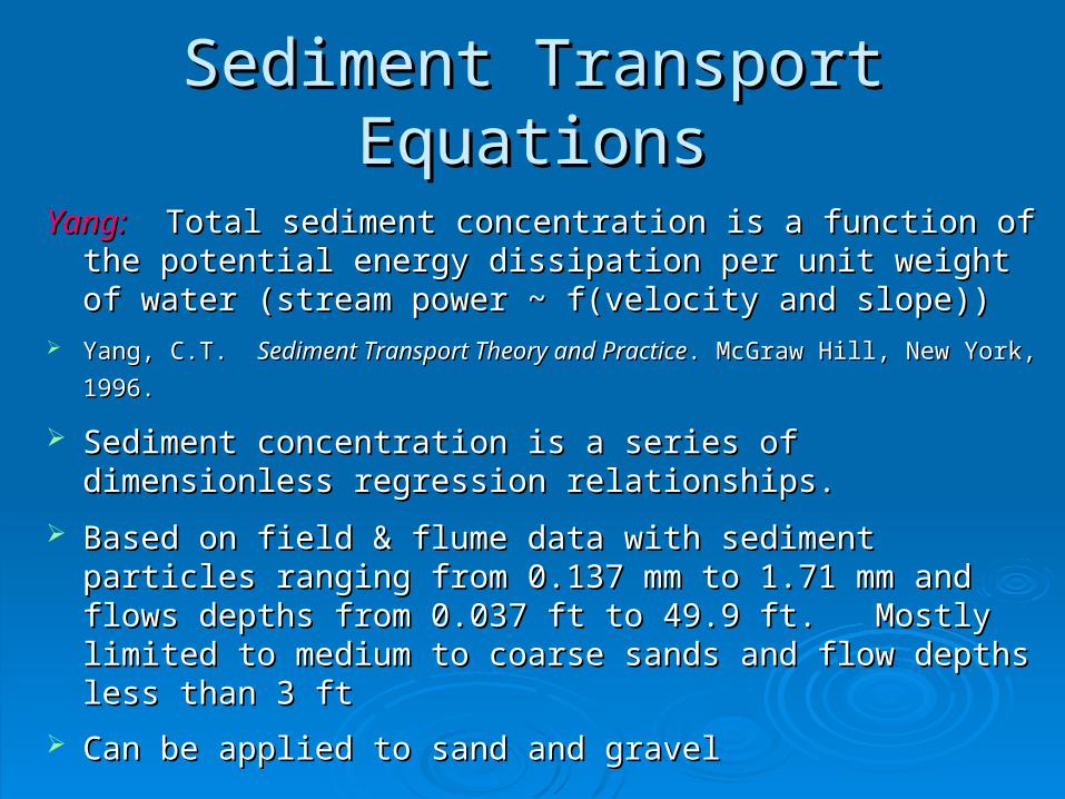
Yang:Yang: Total sediment concentration is a function of the Total sediment concentration is a function of the potential energy dissipation per unit weight of water (stream potential energy dissipation per unit weight of water (stream power ~ f(velocity and slope)) power ~ f(velocity and slope))

Yang, C.T. Yang, C.T. Sediment Transport Theory and PracticeSediment Transport Theory and Practice. McGraw Hill, New York, . McGraw Hill, New York,

1996.1996.

Sediment concentration is a series of dimensionless Sediment concentration is a series of dimensionless regression relationships. regression relationships.

Based on field & flume data with sediment particles ranging Based on field & flume data with sediment particles ranging from 0.137 mm to 1.71 mm and flows depths from 0.037 ft to from 0.137 mm to 1.71 mm and flows depths from 0.037 ft to 49.9 ft. Mostly limited to medium to coarse sands and flow 49.9 ft. Mostly limited to medium to coarse sands and flow depths less than 3 ft depths less than 3 ft

Can be applied to sand and gravelCan be applied to sand and gravel


Parker-Klingeman-McLean Parker-Klingeman-McLean developed and developed and tested using gravel or sandy gravel tested using gravel or sandy gravel transport data. transport data.

Applied to a large number of different Applied to a large number of different gravel-bed rivers.gravel-bed rivers.

Sediment Transport EquationsSediment Transport EquationsParker-Klingeman-McLeanParker-Klingeman-McLean: computes transport rates on the : computes transport rates on the

basis of a single grain size: the median grain size of the basis of a single grain size: the median grain size of the substrate, D50substrate, D50

Parker, G.; Klingeman, P.C.; McLean, D.L. 1982. Bedload and Parker, G.; Klingeman, P.C.; McLean, D.L. 1982. Bedload and size distribution in paved gravel bed streams. size distribution in paved gravel bed streams. Journal of Journal of Hydraulics DivisionHydraulics Division, ASCE. 108: 544-571., ASCE. 108: 544-571.

Recognizes role of armor layer in bed load transport rates.Recognizes role of armor layer in bed load transport rates.


Van Rijn:Van Rijn: Computes suspended load and bed load Computes suspended load and bed load separately. separately.

Van Rijn, L.C., Sediment Transport, Part I: Bed load transport, Van Rijn, L.C., Sediment Transport, Part I: Bed load transport, J. Hyd. Eng.J. Hyd. Eng., ASCE, , ASCE, no 10. 1984ano 10. 1984a

Van Rijn, L.C., Sediment Transport, Part II: Suspended load transport, Van Rijn, L.C., Sediment Transport, Part II: Suspended load transport, J. Hyd. Eng.J. Hyd. Eng., , ASCE, no 11. 1984bASCE, no 11. 1984b

Van Rijn, L.C., Sediment pick-up functions, Van Rijn, L.C., Sediment pick-up functions, J. Hyd. Eng.,J. Hyd. Eng., ASCE, no 10. 1984c ASCE, no 10. 1984c

Estimates sediment concentration.Estimates sediment concentration. Qb = Qs+QbQb = Qs+Qb


Engelund-Hansen Method:Engelund-Hansen Method: Bagnold’s stream power Bagnold’s stream power concept was applied with the similarity principle to concept was applied with the similarity principle to derive a sediment transport function. derive a sediment transport function.

Engelund, F. and Hensen, E. Engelund, F. and Hensen, E. A Monograph on Sediment Transport to Alluvial A Monograph on Sediment Transport to Alluvial StreamsStreams. . Copenhagen: Teknique Vorlag, 1967.Copenhagen: Teknique Vorlag, 1967.

Uses energy slope, velocity, bed shear stress, median Uses energy slope, velocity, bed shear stress, median particle diameter, specific weight of sediment and particle diameter, specific weight of sediment and water, and gravitational acceleration water, and gravitational acceleration

Can be used in both dune bed forms and upper Can be used in both dune bed forms and upper regime (plane bed) Dregime (plane bed) D5050 > 0.15 mm > 0.15 mm

Finite element methodFinite element methodWhy Finite Elements?Why Finite Elements? Solid mathematical theorySolid mathematical theory Meshes can adapt to irregular bottom and Meshes can adapt to irregular bottom and

boundaries boundaries Improved computational efficiencyImproved computational efficiency

Finite element methodFinite element method

Galerkin weighted residual methodGalerkin weighted residual method Converts the PDEs to a system of ODEsConverts the PDEs to a system of ODEs Triangular 3 nodes elementsTriangular 3 nodes elements

RiverFLO-2D finite element methodRiverFLO-2D finite element method

What is new?What is new? Explicit four-step time stepping algorithm Explicit four-step time stepping algorithm

based on matrix lumpingbased on matrix lumping Solve on an element-by-element basisSolve on an element-by-element basis Parallelized Fortran 95 using OpenMPParallelized Fortran 95 using OpenMP


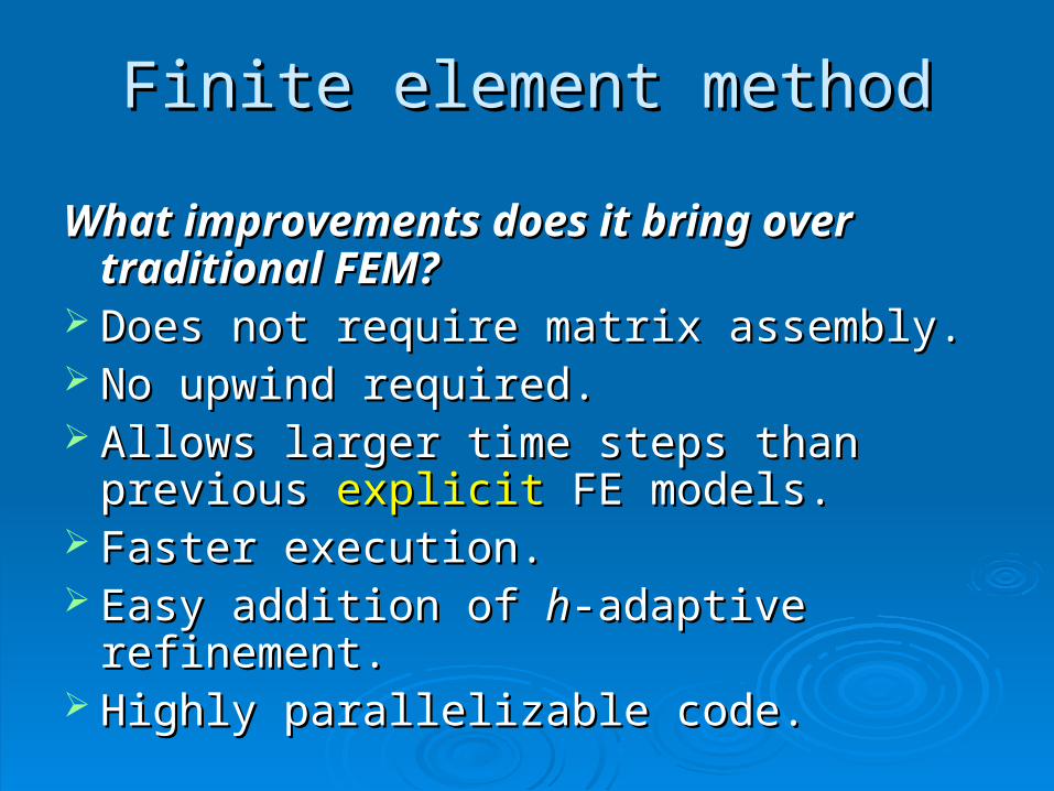
What improvements does it bring over What improvements does it bring over traditional FEM?traditional FEM?

Does not require matrix assembly.Does not require matrix assembly. No upwind required.No upwind required. Allows larger time steps than previous Allows larger time steps than previous

explicitexplicit FE models. FE models. Faster execution.Faster execution. Easy addition of Easy addition of hh-adaptive refinement.-adaptive refinement. Highly parallelizable code.Highly parallelizable code.

Finite element methodFinite element method Linear interpolation functionsLinear interpolation functions

Finite element methodFinite element method System of ODEsSystem of ODEs

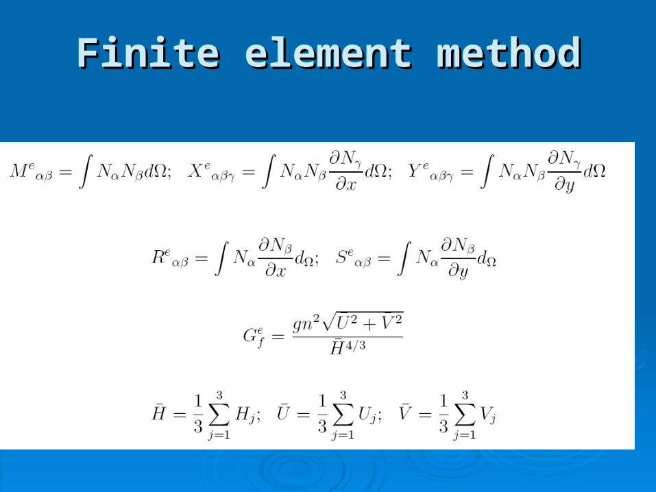
Finite element methodFinite element method Lumping:Lumping:

Lumping improves numerical stability but introduces Lumping improves numerical stability but introduces numerical damping numerical damping

Selective lumping Selective lumping

εε in [0.9,0.98] in [0.9,0.98] is the selective lumping parameter is the selective lumping parameter Selective lumping reduces damping while preserving stabilitySelective lumping reduces damping while preserving stability

FEM. Four-Step time stepping schemeFEM. Four-Step time stepping scheme

FEM. Von Newmann stability analysisFEM. Von Newmann stability analysis

Linearize equations (1D)Linearize equations (1D) Discretize with FEM the linearized Discretize with FEM the linearized

equationsequations Assume form for solution Assume form for solution Substitute in discretized eqn’sSubstitute in discretized eqn’s Spectral radius if amplification matrix less Spectral radius if amplification matrix less

than 1than 1 CFL conditionCFL condition

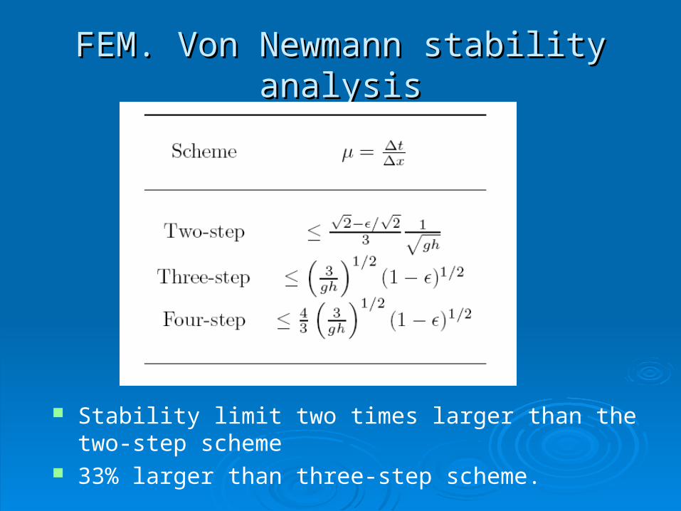
FEM. Von Newmann stability analysisFEM. Von Newmann stability analysis

Stability limit two times larger than the two-step scheme

33% larger than three-step scheme.

Model parallelizationModel parallelization Subdomain decomposition.Subdomain decomposition.

Seamless parallel computation using OpenMPSeamless parallel computation using OpenMP OpenMP: An API for multi-platform shared-memory parallel programming OpenMP: An API for multi-platform shared-memory parallel programming

in C/C++ and Fortran. in C/C++ and Fortran. www.openmp.org, 2009., 2009.

Each Processor/Core computes one subdomainEach Processor/Core computes one subdomain Model speedup depends on number of processors, Model speedup depends on number of processors,

processor cache memory, etc., and is case specific.processor cache memory, etc., and is case specific.

Model Speedup Model Speedup

1.00

1.50

2.00

2.50

3.00

3.50

4.00

4.50

1 2 3 4 5 6 7 8

Spe

edup

Number of Processors/Cores

Treatment of dry-wet areasTreatment of dry-wet areas

At the beginning of each time step all elements are At the beginning of each time step all elements are evaluated to see if they are wet or dry. evaluated to see if they are wet or dry.

A completely dry element is defined when all nodal depths are less than a A completely dry element is defined when all nodal depths are less than a user defined minimum depth Hmin, that can be zero. user defined minimum depth Hmin, that can be zero.

A partially dry element has at least one node, where depth is less than or A partially dry element has at least one node, where depth is less than or equal to Hmin.equal to Hmin.

If one element is completely dry, equations are locally If one element is completely dry, equations are locally modified and only dmodified and only dήή/dt=0, dU/dt=0, dV/dt=0 is solved for /dt=0, dU/dt=0, dV/dt=0 is solved for the element. the element.

If an element is partially dry, the full equations are solved If an element is partially dry, the full equations are solved and velocity components are set to zero for all nodes on the and velocity components are set to zero for all nodes on the element.element.

Water surface elevations are not altered for dry elements.Water surface elevations are not altered for dry elements.

RiverFLO-2D Equations Methods 09-30-09

Documents

Transcript of RiverFLO-2D Equations Methods 09-30-09