RIVERBED -BASED NETWORK MODELING FOR MULTI -BEAM CONCURRENT...

International Journal of Wireless & Mobile Networks (IJWMN) Vol. 9, No. 6, December 2017

DOI: 10.5121/ijwmn.2017.9601 1

RIVERBED-BASED NETWORK MODELING FOR

MULTI-BEAM CONCURRENT TRANSMISSIONS

Ji Qi1, Xin Li1, Shivam Garg

2, Fei Hu

1, Sunil Kumar

2

1Department of Electrical and Computer Engineering, University of Alabama,

Tuscaloosa, AL 2Department of Electrical and Computer Engineering, San Diego State University, San

Diego, CA

ABSTRACT The paper presents a Riverbed simulator implementation with both routing and medium access control

(MAC) protocols for mobile ad-hoc network wireless networks with multi-beam smart antennas (MBSAs).

As one of the latest promising antenna techniques, MBSAs can achieve concurrent transmissions /

receptions in multiple directions/beams. Thus it can significantly improve the network throughput.

However, so far there is still no accurate network simulator that can measure the MBSA-based

routing/MAC protocol performance. In this paper, we describe the simulation models with the

implementation of MBSA antenna model in physical layer, MAC layer, and routing layer protocols, all in

Riverbed Modeler. We will compare two routing scenarios, i.e., multi-hop diamond routing scenario and

multi-path pipe routing. We will analyze the network performance for those two scenarios and illustrate the

advantages of using MBSAs in wireless networks.

INDEX TERMS

Multi-beam Smart Antennas (MBSAs), Medium Access Control (MAC), Multi-path routing, Riverbed

Modeler.

I. INTRODUCTION

Today the most popular antenna used in wireless devices is the omni directional antenna.

However, such an antenna radiates energy in all the 360-degree spaces, which results in poor

spatial reuse and strong interference among the neighboring nodes. A promising new type of

antenna, called multi-beam smart antenna (MBSA), can concurrently send data to different

angles/beams and sperate the signal domains between the beams. Thus a MBSA could

significantly improve the spatial reuse and the network throughput. By using MBSAs, a node can

achieve concurrent packet reception (CPR) and concurrent packet transmission (CPT). This

means that ideally the node throughput can be enlarged for N times if there are N beams in the

MBSA, compared to general directional antenna with only one beam.

A mobile ad-hoc network (MANET) [1] consists of mobile nodes which communicate with each

other either directly or relying on relay nodes, but without the use of fixed infrastructure or

centralized administration. The nodes have to execute all network functions such as discovering

the network topology or delivering packets via routing protocols. In MANETs every node is a

potential router. Therefore, routing scheme plays an important role for data forwarding in

MANETs where each mobile node can act as a relay in addition to being a source or destination


2

node [2], [3]. Many routing protocols have been proposed to provide data forwarding services for

MANETs. They can be classified as reactive (on-demand) or proactive (the routing path is always

ready for use). A popular reactive protocol is Ad-Hoc on Demand Distance Vector Routing

Protocol (AODV) [4], and a popularly used proactive scheme is Optimized Link State Routing

Protocol (OLSR) [5]. Some existed routing protocols are enumerated in Fig. 1.

Fig. 1. MANET routing protocols

However, very little research has been conducted on MBSAoriented routing or MAC design for

MANETs. MBSAs can bring many benefits to MANET (such as improving data throughput and

shorten routing delay). But the routing/MAC design for MBSA-based networks also raises some

challenging issues. Here we list a few:

1) If using MBSAs, it is prohibitive to make some of the beams operate in transmission (Tx)

mode while others in reception (Rx) mode. In other words, a node should work either as a

transmitter (with all beams in Tx mode) or a receiver (all in Rx mode). It can not send AND

receive packets at the same time. This is mainly because that its antenna design requires that all

beams’ coefficient vectors be determined in the same control matrix. If Tx and Rx modes are

mixed at the same time, the side lobe of those beams working in Tx mode would seriously

interfere with those beams working in Rx mode due to the energy leakage issues.

2) In order to make full use of the benefit of the concurrent transmissions, all neighboring nodes

(especially the nodes within two hops of range) need to be carefully coordinated. Clock/schedule

synchronization turns out to be a serious issue in MBSA-based networks since it cannot just rely

on the use of request-to-send (RTS)/ clear-to-send (CTS) and acknowledge (ACK) messages.

3) Despite the fact that theoretically a MBSA is able to enlarge the node capacity by N times

(where N is the number of beams of the antenna), a specific MAC protocol is needed to control

the beam schedule as well as the beam-based distributed coordination function (DCF). Most of

the conventional MAC protocols are designed for omnidirectional or single-directional nodes, and

use traditional IEEE 802.11 protocols. However, to take advantage of the high capability of

multi-beam transmissions, a new MAC scheme is needed.

Riverbed Modeler (formerly called OPNET) [6] is a popular network simulation software

package. It provides a flexible and accurate simulation platform for evaluating the performance of

verious networking protocols. Riverbed Modeler provides the access to a rich set of API calls.

The process models of the network nodes are implemented in the programming language called


3

Proto-C, and are constructed by using finite state machine (FSM)-based transition diagrams. The

features of Riverbed software allow the test of standardized protocols (such as TCP/IP), as well as

the development of new communication protocols and networking paradigms. We have used

Riverbed Modeler version 18.5 to implement multi-path data transmission schemes with MBSAs

and comprehensively analyzed its routing performance.

This paper takes the first step to build the Riverbed-based MBSA-oriented network simulator.

Riverbed is a commercialized network simulation tool, and can more accurately reflect the actual

network performance than other network simulation tools such as ns-3. We will first introduce the

background knowledge of MBSA and Riverbed Modeler, and then summarizes some related

works in Section II. In section III, we will discuss our design of MBSA model and its MAC layer

protocol in Riverbed. In section IV, we provide a detailed description of modeling two multi-path

routing scenarios, followed by the conclusions in Section V.

II. BACKGROUND AND RELATED WORKS

There has been much research work conducted on MANET performance analysis by using

Riverbed (OPNET) Modeler. Agustin Zaballos et al. [7] provided a comparative study about four

routing protocols, i.e., DSR, TORA, AODV and OLSR, for MANETs. Naveen Bilandi and Harsh

K Verma [8] conducted the similar study, and measured the performance of different routing

protocols by using three metrics: delay, network load, and throughput. Sheela Ganesh Thorenoor

[9] presented the implementation process and compared the protocols that are based on distance

vector or link state algorithms.

Vasil Hnatyshin and Hristo Asenov [10] introduced the design and implementation of GeoAODV

routing protocol in OPNET Modeler, which used Global Positioning System (GPS) coordinates to

search the area where a path to the destination is likely to be located. Rani Al-Maharmah et al.

[11] provided an overview of OPNET Modeler architecture and described a practical

methodology to add new MANET routing protocols to OPNET Modeler by using the Multi-

Aware Cluster Head Maintenance (MACHM). Regarding antenna design, John A. Stine [12]

described the details of how to build models of adaptive antennas in OPNET by using the radio

process model and radio pipeline stages.

However, none of the above studies involves the MBSAbased protocol test, which requires

special concurrent communication protocols in different layers. For example, in physical layer, a

new antenna model needs to be built and added to the Riverbed library. The MAC layer needs to

call such an antenna model to implement the synchronized collision avoidance control, and the

routing layer should use some sort of multipath routing with multi-beam coordinations to fully

utilize the features (CPT/CPR) of MBSAs. In the following discussions we will provide our

Riverbed implementation details for the above aspects.

III. NETWORK SIMULATION ARCHITECTURE IN RIVERBED MODELER

In Riverbed Modeler, the network architecture is modeled as a layered structure. The process

domain is in the lowest layer, which contains the actual functions of the modeled protocols. The

process models consist of state transition diagrams as well as some blocks of C codes. Each

process is designed to respond to different events/interrupts. We can dynamically create child

processes for each process.


4

The node domain is responsible for creating the models of individual devices and relies on the

process models to simulate the behaviors of different function modules. There are some basic

building blocks including processors, queues, and transceivers. Processors are fully

programmable via their process model. The Queue modules can buffer and manage data packets,

and the transceivers are the interfaces of the node.

The top layer, i.e., network domain, represents a complete system of interconnected devices.

Besides nodes, network models also have links and subnets. Either point-to-point or bus links can

be used in the networks.

In Riverbed Modeler, packets are the information-carrying entities that circulate among system

components. We can dynamically create and destroy the packets during the simulations. Packets

can either be unformatted or formatted. Unformatted packets have no user-defined data fields

while formatted packets have one or more fields. A single system may rely on multiple types of

packets with different formats.

The simulations in Riverbed Modeler are event-driven. In this programming paradigm, events are

specific activities that occur at a certain time, and the simulation time advances when an event

occurs. Event-driven method is naturally suited to the applications whose control flow are based

on the internal or external events. But the accuracy of results is limited by the sampling

resolution.

Riverbed Modeler allows a realistic estimation of the performance and behavior for the executed

simulations. It has several mechanisms to collect the data. The output data is generated after each

simulation. Desired statistics are explicitly recorded in the appropriate output files. The

programmer can specify a list of probes, each of which indicates that a particular statistic should

be collected in this run. Advanced forms of probes can be defined by the users through its probe

editor.

IV. MBSA MODEL AND MAC LAYER DESIGN

A. Multi-beam Antenna

Figure 2 illustrates the typical single-beam antenna as well as MBSA models. As shown in Fig.

2(a), a single beam has one main lobe and several side lobes. The side lobes cover only small

areas, and are thus not capable of establishing effective communications. The main lobe covers a

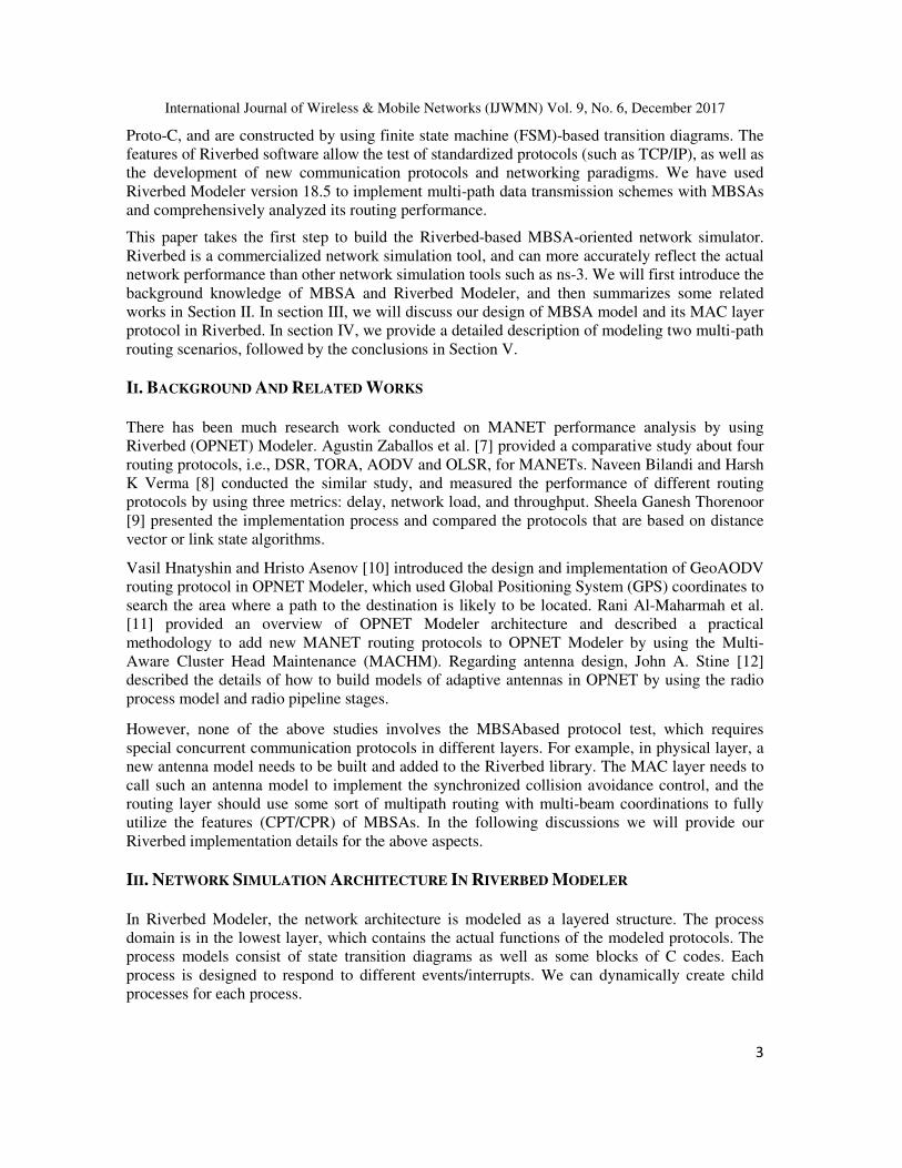
much larger area with a long propagation distance. In Fig. 2(b), however, we could see multiple

main lobes (marked by blue color) face different directions. A node can dispatch different packets

in multiple beams concurrently. Compared with MIMO antennas, MBSAs have much lower

manufacturing cost and control complexity.

(a) single-beam


5

(b) multi-beam antennas

Fig. 2. An illustration of (a) single-beam, and (b) multi-beam antennas.

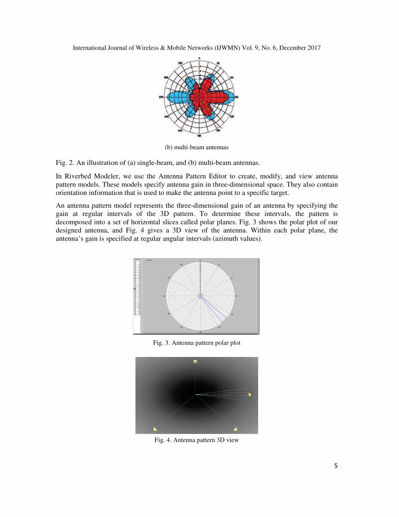
In Riverbed Modeler, we use the Antenna Pattern Editor to create, modify, and view antenna

pattern models. These models specify antenna gain in three-dimensional space. They also contain

orientation information that is used to make the antenna point to a specific target.

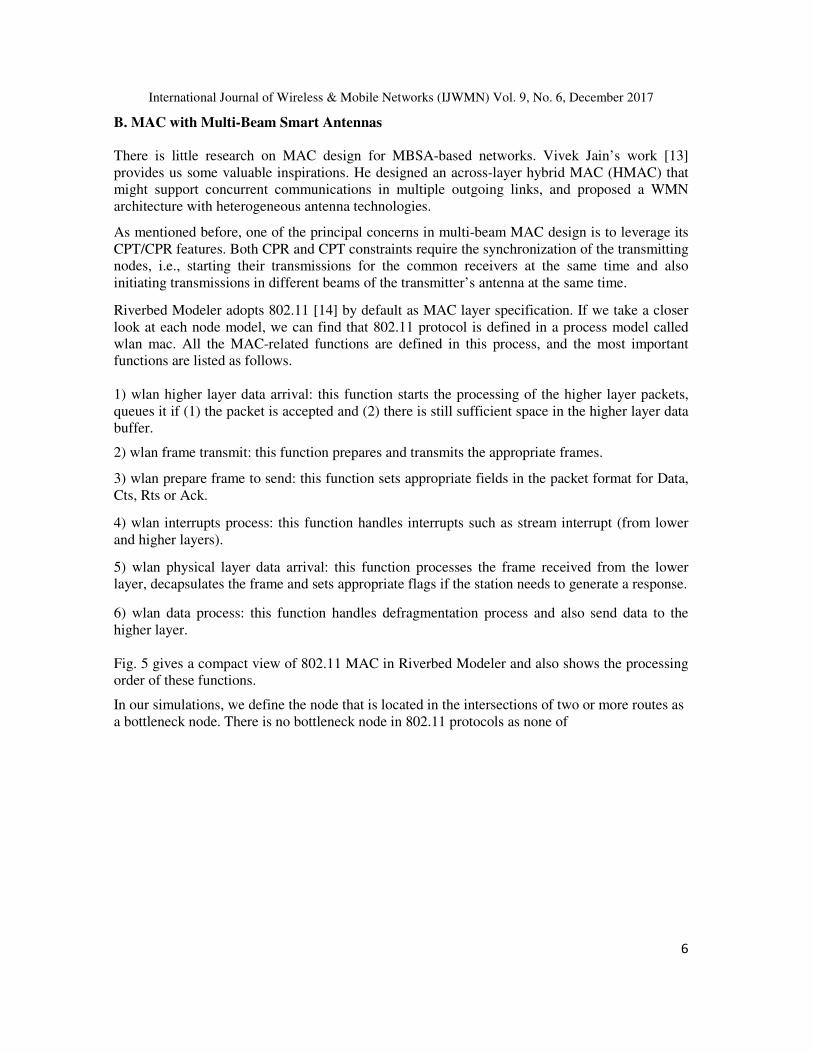
An antenna pattern model represents the three-dimensional gain of an antenna by specifying the

gain at regular intervals of the 3D pattern. To determine these intervals, the pattern is

decomposed into a set of horizontal slices called polar planes. Fig. 3 shows the polar plot of our

designed antenna, and Fig. 4 gives a 3D view of the antenna. Within each polar plane, the

antenna’s gain is specified at regular angular intervals (azimuth values).

Fig. 3. Antenna pattern polar plot

Fig. 4. Antenna pattern 3D view


6

B. MAC with Multi-Beam Smart Antennas

There is little research on MAC design for MBSA-based networks. Vivek Jain’s work [13]

provides us some valuable inspirations. He designed an across-layer hybrid MAC (HMAC) that

might support concurrent communications in multiple outgoing links, and proposed a WMN

architecture with heterogeneous antenna technologies.

As mentioned before, one of the principal concerns in multi-beam MAC design is to leverage its

CPT/CPR features. Both CPR and CPT constraints require the synchronization of the transmitting

nodes, i.e., starting their transmissions for the common receivers at the same time and also

initiating transmissions in different beams of the transmitter’s antenna at the same time.

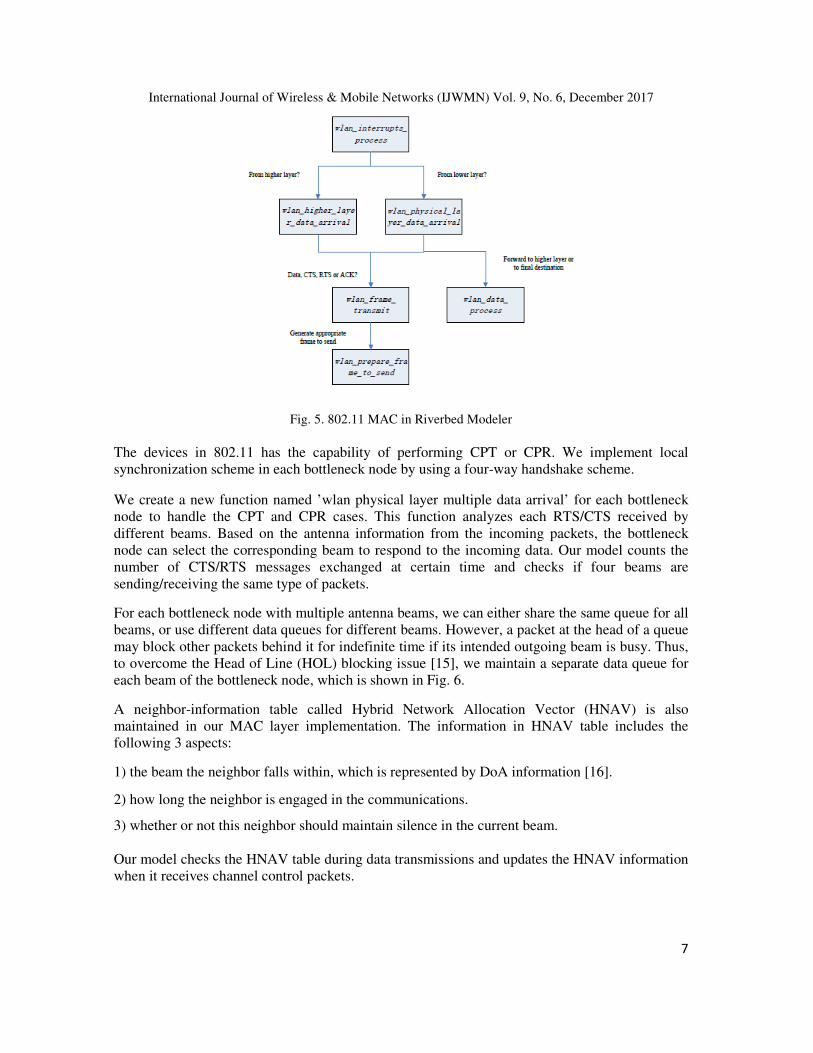
Riverbed Modeler adopts 802.11 [14] by default as MAC layer specification. If we take a closer

look at each node model, we can find that 802.11 protocol is defined in a process model called

wlan mac. All the MAC-related functions are defined in this process, and the most important

functions are listed as follows.

1) wlan higher layer data arrival: this function starts the processing of the higher layer packets,

queues it if (1) the packet is accepted and (2) there is still sufficient space in the higher layer data

buffer.

2) wlan frame transmit: this function prepares and transmits the appropriate frames.

3) wlan prepare frame to send: this function sets appropriate fields in the packet format for Data,

Cts, Rts or Ack.

4) wlan interrupts process: this function handles interrupts such as stream interrupt (from lower

and higher layers).

5) wlan physical layer data arrival: this function processes the frame received from the lower

layer, decapsulates the frame and sets appropriate flags if the station needs to generate a response.

6) wlan data process: this function handles defragmentation process and also send data to the

higher layer.

Fig. 5 gives a compact view of 802.11 MAC in Riverbed Modeler and also shows the processing

order of these functions.

In our simulations, we define the node that is located in the intersections of two or more routes as

a bottleneck node. There is no bottleneck node in 802.11 protocols as none of


7

Fig. 5. 802.11 MAC in Riverbed Modeler

The devices in 802.11 has the capability of performing CPT or CPR. We implement local

synchronization scheme in each bottleneck node by using a four-way handshake scheme.

We create a new function named ’wlan physical layer multiple data arrival’ for each bottleneck

node to handle the CPT and CPR cases. This function analyzes each RTS/CTS received by

different beams. Based on the antenna information from the incoming packets, the bottleneck

node can select the corresponding beam to respond to the incoming data. Our model counts the

number of CTS/RTS messages exchanged at certain time and checks if four beams are

sending/receiving the same type of packets.

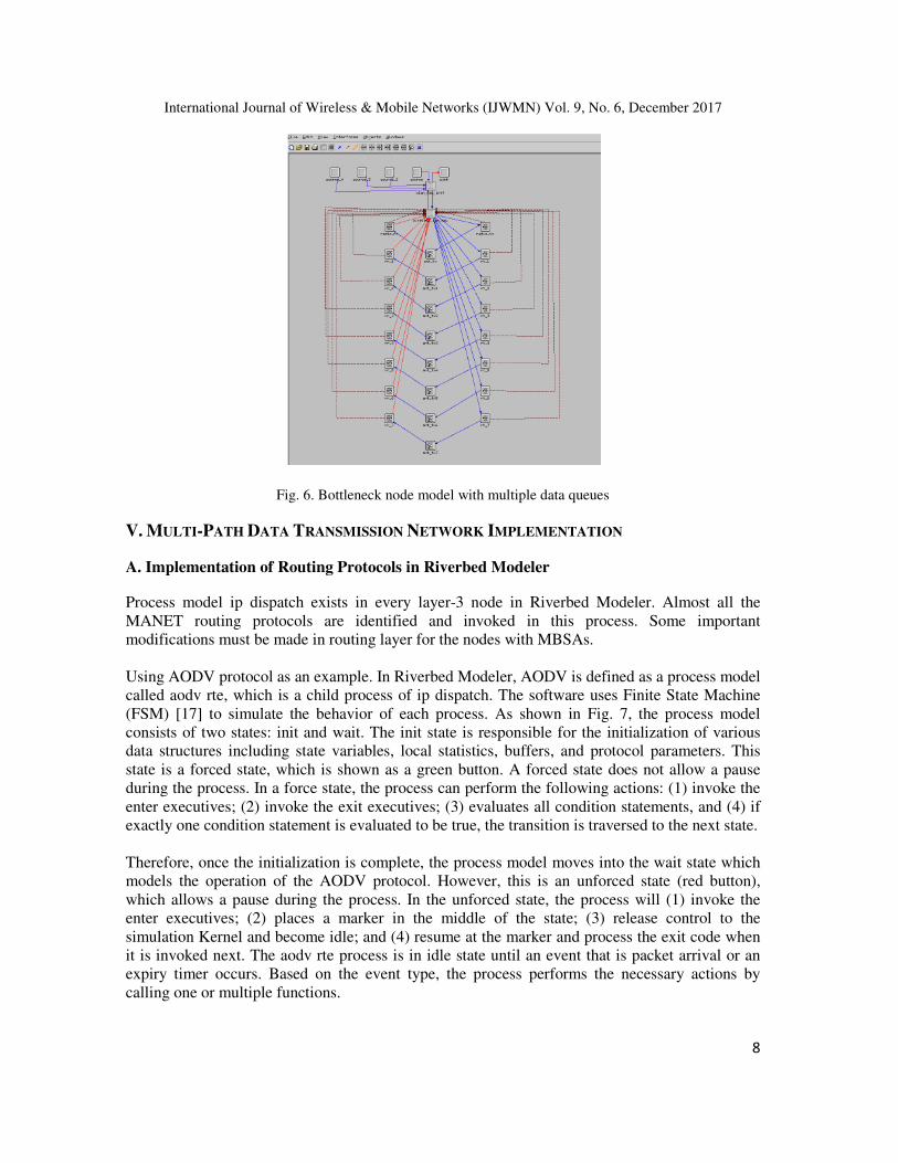
For each bottleneck node with multiple antenna beams, we can either share the same queue for all

beams, or use different data queues for different beams. However, a packet at the head of a queue

may block other packets behind it for indefinite time if its intended outgoing beam is busy. Thus,

to overcome the Head of Line (HOL) blocking issue [15], we maintain a separate data queue for

each beam of the bottleneck node, which is shown in Fig. 6.

A neighbor-information table called Hybrid Network Allocation Vector (HNAV) is also

maintained in our MAC layer implementation. The information in HNAV table includes the

following 3 aspects:

1) the beam the neighbor falls within, which is represented by DoA information [16].

2) how long the neighbor is engaged in the communications.

3) whether or not this neighbor should maintain silence in the current beam.

Our model checks the HNAV table during data transmissions and updates the HNAV information

when it receives channel control packets.


8

Fig. 6. Bottleneck node model with multiple data queues

V. MULTI-PATH DATA TRANSMISSION NETWORK IMPLEMENTATION

A. Implementation of Routing Protocols in Riverbed Modeler

Process model ip dispatch exists in every layer-3 node in Riverbed Modeler. Almost all the

MANET routing protocols are identified and invoked in this process. Some important

modifications must be made in routing layer for the nodes with MBSAs.

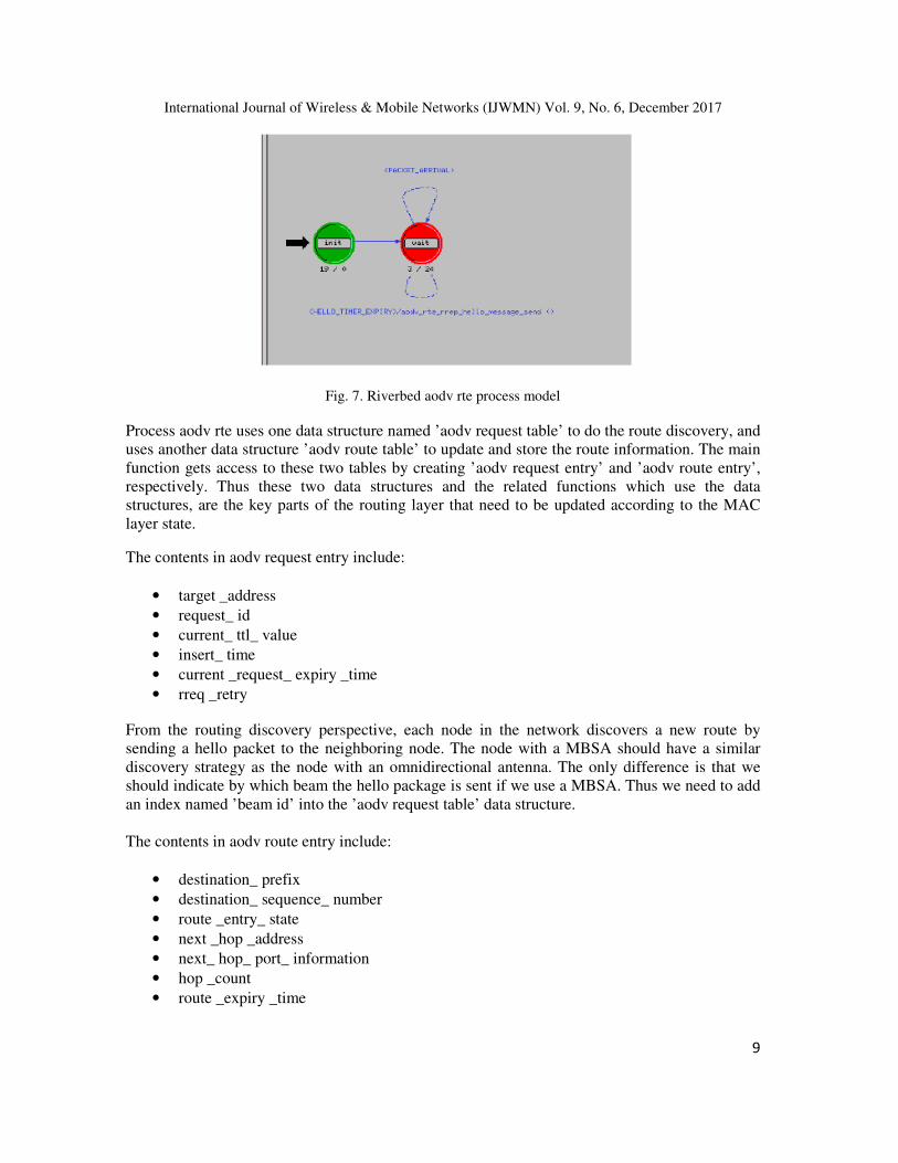
Using AODV protocol as an example. In Riverbed Modeler, AODV is defined as a process model

called aodv rte, which is a child process of ip dispatch. The software uses Finite State Machine

(FSM) [17] to simulate the behavior of each process. As shown in Fig. 7, the process model

consists of two states: init and wait. The init state is responsible for the initialization of various

data structures including state variables, local statistics, buffers, and protocol parameters. This

state is a forced state, which is shown as a green button. A forced state does not allow a pause

during the process. In a force state, the process can perform the following actions: (1) invoke the

enter executives; (2) invoke the exit executives; (3) evaluates all condition statements, and (4) if

exactly one condition statement is evaluated to be true, the transition is traversed to the next state.

Therefore, once the initialization is complete, the process model moves into the wait state which

models the operation of the AODV protocol. However, this is an unforced state (red button),

which allows a pause during the process. In the unforced state, the process will (1) invoke the

enter executives; (2) places a marker in the middle of the state; (3) release control to the

simulation Kernel and become idle; and (4) resume at the marker and process the exit code when

it is invoked next. The aodv rte process is in idle state until an event that is packet arrival or an

expiry timer occurs. Based on the event type, the process performs the necessary actions by

calling one or multiple functions.


9

Fig. 7. Riverbed aodv rte process model

Process aodv rte uses one data structure named ’aodv request table’ to do the route discovery, and

uses another data structure ’aodv route table’ to update and store the route information. The main

function gets access to these two tables by creating ’aodv request entry’ and ’aodv route entry’,

respectively. Thus these two data structures and the related functions which use the data

structures, are the key parts of the routing layer that need to be updated according to the MAC

layer state.

The contents in aodv request entry include:

• target _address

• request_ id

• current_ ttl_ value

• insert_ time

• current _request_ expiry _time

• rreq _retry

From the routing discovery perspective, each node in the network discovers a new route by

sending a hello packet to the neighboring node. The node with a MBSA should have a similar

discovery strategy as the node with an omnidirectional antenna. The only difference is that we

should indicate by which beam the hello package is sent if we use a MBSA. Thus we need to add

an index named ’beam id’ into the ’aodv request table’ data structure.

The contents in aodv route entry include:

• destination_ prefix

• destination_ sequence_ number

• route _entry_ state

• next _hop _address

• next_ hop_ port_ information

• hop _count

• route _expiry _time


10

Similarly, we need to add an index named ’beam _id’ into the ’aodv_ route_ table’ data structure.

Both table data structures are defined in the header file ’aodv.h’. Here ’aodv _request _entry’ is

further divided into two data structures, i.e., AodvT _Orig_ Request _Entry’ and ’AodvT_

Forward _Request_ Entry’.

We also need to change the packet format of ’RREQ’ and ’RREP’, and put ’beam id’ information

in each packet. All the packet formats are defined in the header file ’aodv_ pkt _support.h’ while

all the packet creation functions are defined in the file ’aodv _pkt_ support.ex.c’. To change the

format of ’RREQ’ and ’RREP’ messages, we need to modify the corresponding functions ’aodv

_pkt _support _rreq _option _create’ and ’aodv _pkt_ support_ rrep _option _create’.

The file ’aodv _request_ table.ex.c’ contains all the operation functions of the request table.

When we send a new route request, we need to add it into the request table. We also need to

change the related functions ’aodv _request_ table_ orig_ rreq_ insert’ and ’aodv_ request _table

_forward _rreq _insert’.

For the control functions of the routing table, we only need to change the function ’aodv _route_

table_ entry _create’ function which is defined in ”aodv_ route_ table.ex.c’.

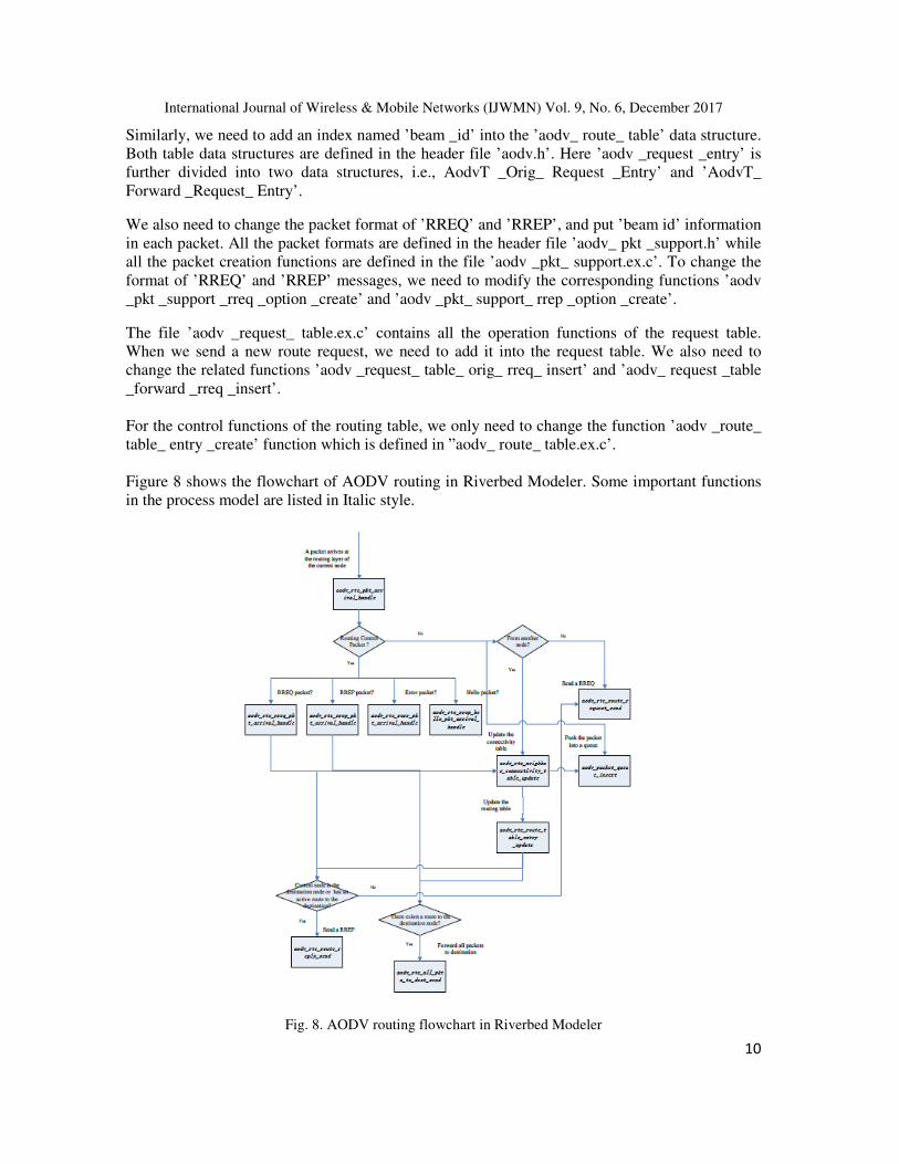
Figure 8 shows the flowchart of AODV routing in Riverbed Modeler. Some important functions

in the process model are listed in Italic style.

Fig. 8. AODV routing flowchart in Riverbed Modeler


11

We can always obtain the beam status information (such as orientation) from MAC and physical

layers. If a node has occupied the channel and known its destination node in the MAC layer, we

can easily determine which beam is used to send the data. Thus we can pass these parameters

from lower layers to higher layers through the node model.

Based on the definition of the OSI 7-layers network model [18], routing layer is located in the

network layer, which is further divided into 2 parts: the lower layer is routing layer and the upper

layer is IP layer. In Riverbed Modeler, each node (either a transmitter or a receiver) should create

a network interface before communicating with each other. And each interface needs to be

assigned with an IP address. From Fig. 6 we can see that in MAC layer we have attached four

pairs of ’radio _txrx’ models to one node. Riverbed assigns an IP address to each interface by

default. Thus here we have four different addresses for one node, which is disallowed in a typical

network. To solve the ’IP addressing’ problem, we combine all the four pairs of radio interfaces

as an entire entity. They are assigned to the same IP address and are always treated equally. All

the modifications of IP assignment functions are located in the file ’ip_ auto_ addr_ sup v4.ex.c’.

B. Multi-hop Diamond Routing Scenario

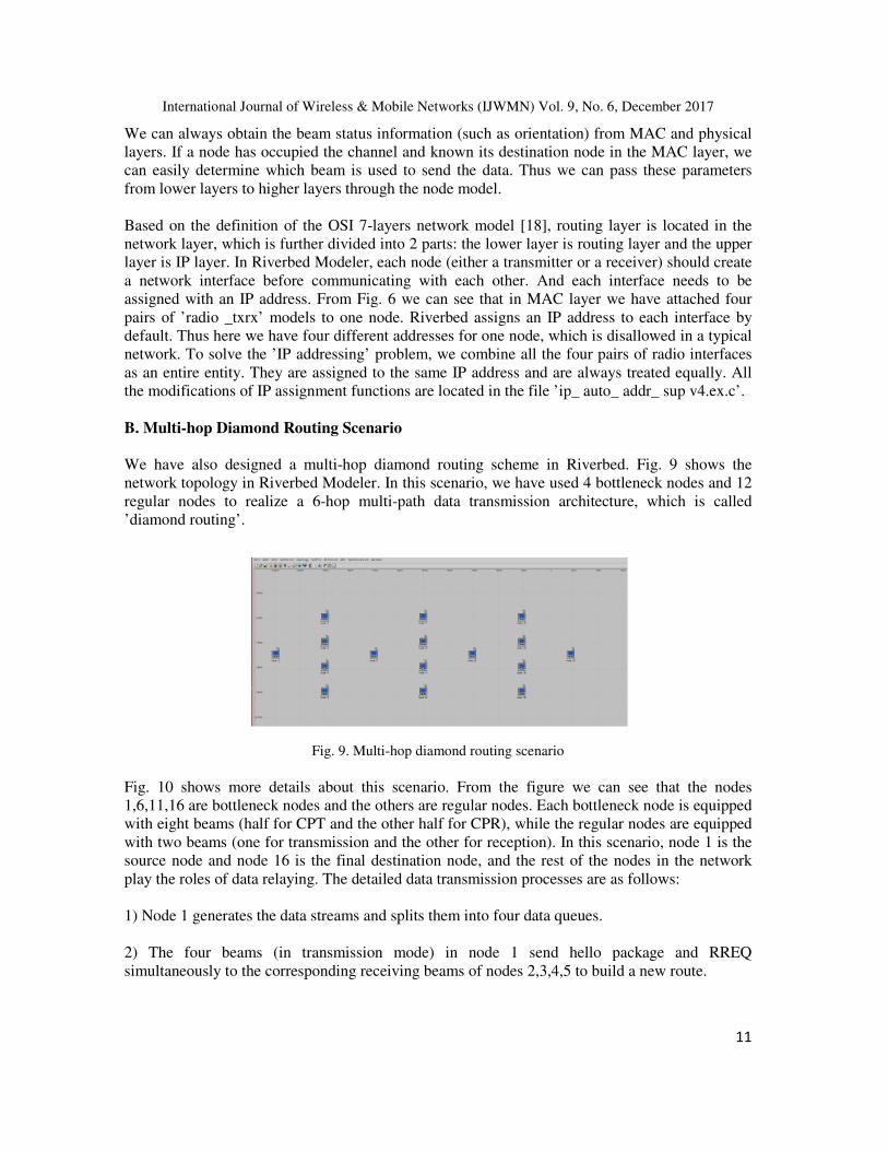
We have also designed a multi-hop diamond routing scheme in Riverbed. Fig. 9 shows the

network topology in Riverbed Modeler. In this scenario, we have used 4 bottleneck nodes and 12

regular nodes to realize a 6-hop multi-path data transmission architecture, which is called

’diamond routing’.

Fig. 9. Multi-hop diamond routing scenario

Fig. 10 shows more details about this scenario. From the figure we can see that the nodes

1,6,11,16 are bottleneck nodes and the others are regular nodes. Each bottleneck node is equipped

with eight beams (half for CPT and the other half for CPR), while the regular nodes are equipped

with two beams (one for transmission and the other for reception). In this scenario, node 1 is the

source node and node 16 is the final destination node, and the rest of the nodes in the network

play the roles of data relaying. The detailed data transmission processes are as follows:

1) Node 1 generates the data streams and splits them into four data queues.

2) The four beams (in transmission mode) in node 1 send hello package and RREQ

simultaneously to the corresponding receiving beams of nodes 2,3,4,5 to build a new route.


12

3) The nodes 2,3,4,5 exchange RTS and CTS with node 1 simultaneously to start data

transmissions.

4) Node 1 sends its data through 4 beams to nodes 2,3,4,5 simultaneously.

5) Nodes 2,3,4,5 receive the data, decode the data packet head, and analyze the final destination.

6) The other beams of nodes 2,3,4,5 will send hello package and RREQ again simultaneously to

the corresponding receiving beams of node 6 to build a new route.

7) Node 6 exchanges RTS and CTS with nodes 2,3,4,5 simultaneously to start another hop of data

transmission.

8) Nodes 2,3,4,5 send its data to node 6 simultaneously.

9) Node 6 receives the data, decodes the data packet head and analyzes the final destination.

10) Node 6 will again, build a new route and forward the received data to nodes 7,8,9,10

simultaneously, until all the data reached node 16.

The bottleneck nodes 6 and 11, which serve as the relay nodes in this scenario, require packet

distribution and beam switching schedule. Local synchronization is also required here, since all

the eight beams of the node will be used during the data transmissions.

To make things more clear, we set a packet relay scheme in each bottleneck relay node. Taking

node 6 as an example, from Fig. 10 we can obtain the position and index of each antenna beam.

Each packet from node 2, which is received by beam 1, will be pushed into the outgoing queue of

beam 5. Then the packets will be sent to node 7. Similarly, the packets received by beam 2 will

go to beam 6, etc. This process helps us better balance the traffic loads in different links.

Our packet relay scheme is mainly implemented in process wlan _mac. For each received packet,

the relay node will first perform the address resolution. After that the packet will be pushed back

to the MAC layer. As mentioned in Section IV, the function ’wlan_ data_ process’ will handle the

packets which need to be forwarded to the next hop. We have rebuilt the function ’wlan _data_

process’. In this new function, we first get the ’beam_ id” of each incoming packet and then push

it into the corresponding queue by using the function ’wlan _hlpk_ enqueue’.We then add a

’queue_ id’ to the original ’wlan _hlpk _enqueue’ function, which indicates the index of different

queues.

Moreover, we need to carefully setup the time schedules because CPT and CPR cannot occur

simultaneously, i.e., they should occur alternatively in the same node. For example, node 6 will

first receive four data packets from nodes 2,3,4,5. Although it is a concurrent transmission, some

time deviations may still occur. Considering the different queueing delays and data amounts in

each beam, we need to make the ’fastest’ beam wait for the ’slowest’ beam. Thus here we split

the timeline into several small time slots. In each slot only half of the beams work, either in CPT

or CPR mode.


13

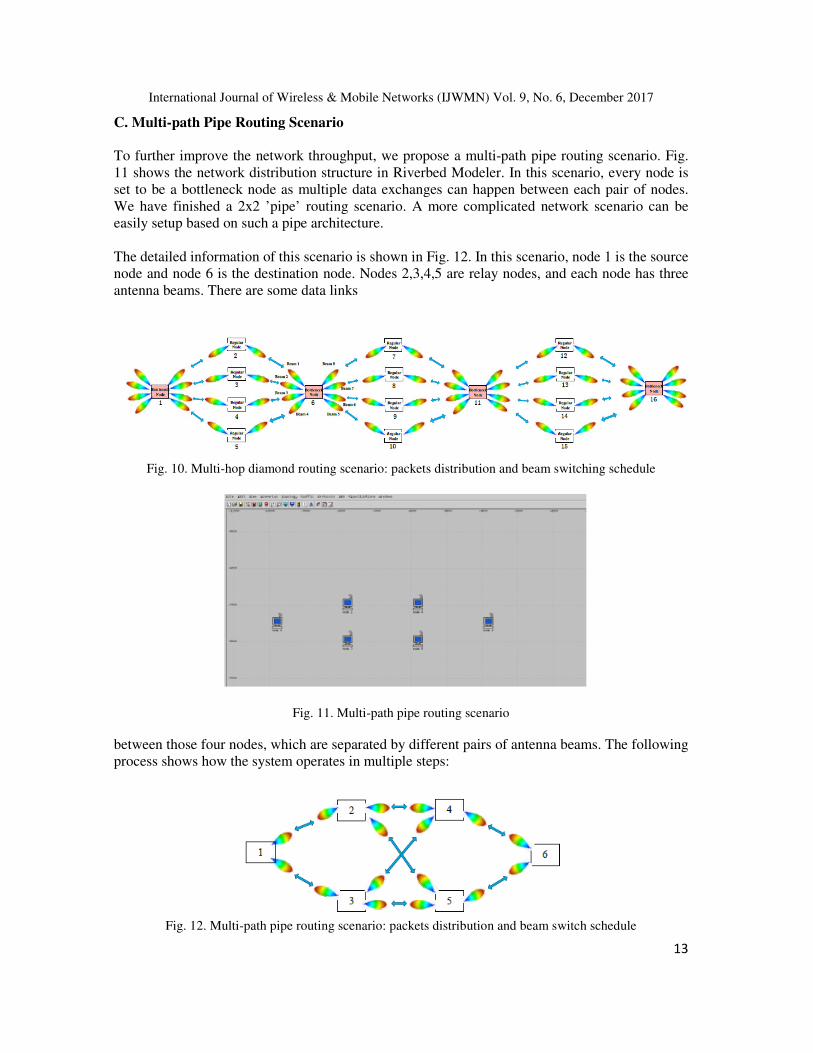
C. Multi-path Pipe Routing Scenario

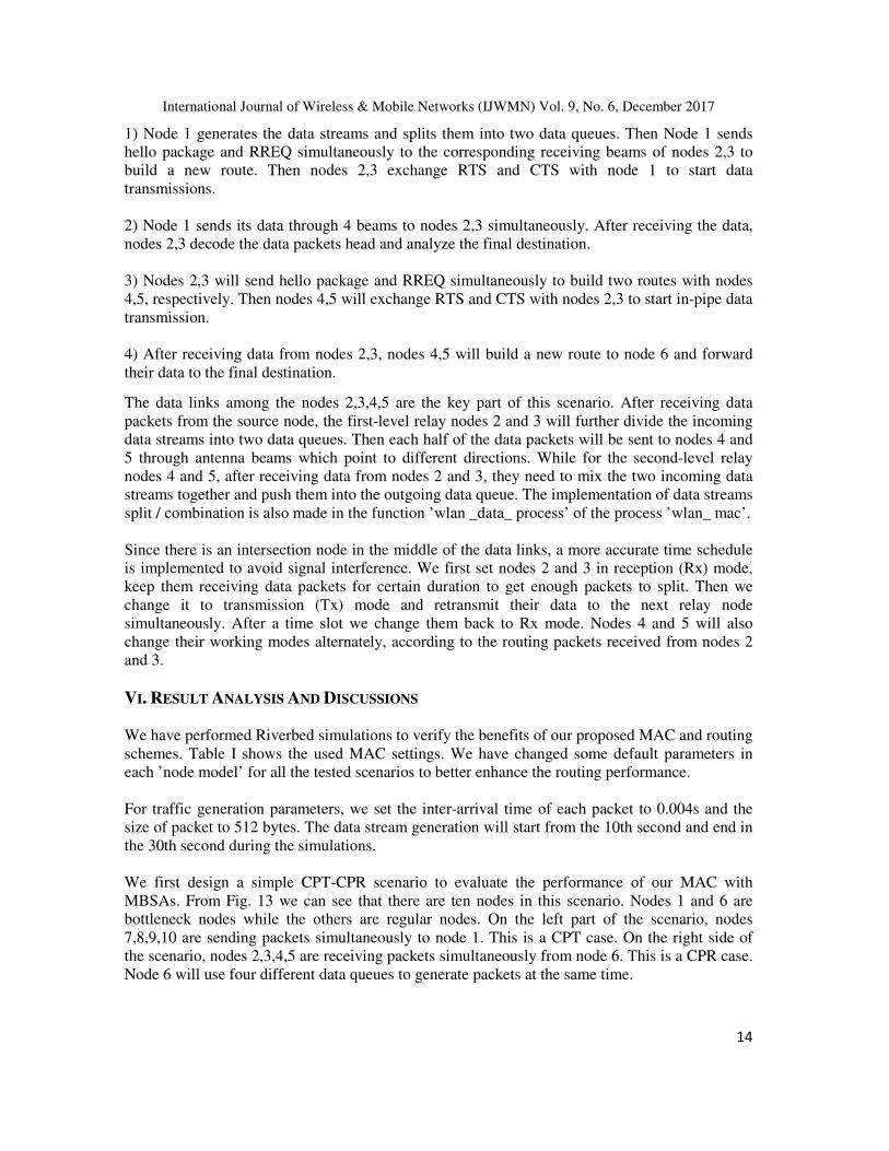
To further improve the network throughput, we propose a multi-path pipe routing scenario. Fig.

11 shows the network distribution structure in Riverbed Modeler. In this scenario, every node is

set to be a bottleneck node as multiple data exchanges can happen between each pair of nodes.

We have finished a 2x2 ’pipe’ routing scenario. A more complicated network scenario can be

easily setup based on such a pipe architecture.

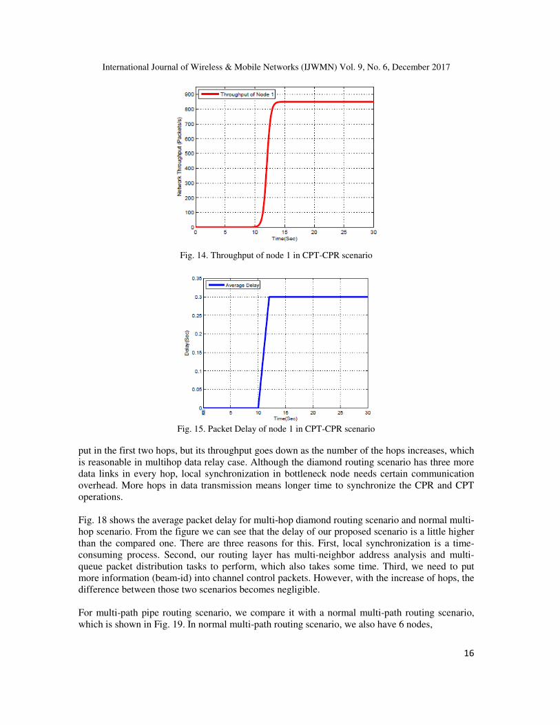
The detailed information of this scenario is shown in Fig. 12. In this scenario, node 1 is the source

node and node 6 is the destination node. Nodes 2,3,4,5 are relay nodes, and each node has three

antenna beams. There are some data links

Fig. 10. Multi-hop diamond routing scenario: packets distribution and beam switching schedule

Fig. 11. Multi-path pipe routing scenario

between those four nodes, which are separated by different pairs of antenna beams. The following

process shows how the system operates in multiple steps:

Fig. 12. Multi-path pipe routing scenario: packets distribution and beam switch schedule


14

1) Node 1 generates the data streams and splits them into two data queues. Then Node 1 sends

hello package and RREQ simultaneously to the corresponding receiving beams of nodes 2,3 to

build a new route. Then nodes 2,3 exchange RTS and CTS with node 1 to start data

transmissions.

2) Node 1 sends its data through 4 beams to nodes 2,3 simultaneously. After receiving the data,

nodes 2,3 decode the data packets head and analyze the final destination.

3) Nodes 2,3 will send hello package and RREQ simultaneously to build two routes with nodes

4,5, respectively. Then nodes 4,5 will exchange RTS and CTS with nodes 2,3 to start in-pipe data

transmission.

4) After receiving data from nodes 2,3, nodes 4,5 will build a new route to node 6 and forward

their data to the final destination.

The data links among the nodes 2,3,4,5 are the key part of this scenario. After receiving data

packets from the source node, the first-level relay nodes 2 and 3 will further divide the incoming

data streams into two data queues. Then each half of the data packets will be sent to nodes 4 and

5 through antenna beams which point to different directions. While for the second-level relay

nodes 4 and 5, after receiving data from nodes 2 and 3, they need to mix the two incoming data

streams together and push them into the outgoing data queue. The implementation of data streams

split / combination is also made in the function ’wlan _data_ process’ of the process ’wlan_ mac’.

Since there is an intersection node in the middle of the data links, a more accurate time schedule

is implemented to avoid signal interference. We first set nodes 2 and 3 in reception (Rx) mode,

keep them receiving data packets for certain duration to get enough packets to split. Then we

change it to transmission (Tx) mode and retransmit their data to the next relay node

simultaneously. After a time slot we change them back to Rx mode. Nodes 4 and 5 will also

change their working modes alternately, according to the routing packets received from nodes 2

and 3.

VI. RESULT ANALYSIS AND DISCUSSIONS

We have performed Riverbed simulations to verify the benefits of our proposed MAC and routing

schemes. Table I shows the used MAC settings. We have changed some default parameters in

each ’node model’ for all the tested scenarios to better enhance the routing performance.

For traffic generation parameters, we set the inter-arrival time of each packet to 0.004s and the

size of packet to 512 bytes. The data stream generation will start from the 10th second and end in

the 30th second during the simulations.

We first design a simple CPT-CPR scenario to evaluate the performance of our MAC with

MBSAs. From Fig. 13 we can see that there are ten nodes in this scenario. Nodes 1 and 6 are

bottleneck nodes while the others are regular nodes. On the left part of the scenario, nodes

7,8,9,10 are sending packets simultaneously to node 1. This is a CPT case. On the right side of

the scenario, nodes 2,3,4,5 are receiving packets simultaneously from node 6. This is a CPR case.

Node 6 will use four different data queues to generate packets at the same time.


15

Table I Mac Settings In Our Riverbed Simulation

Fig. 13. CPT-CPR scenario

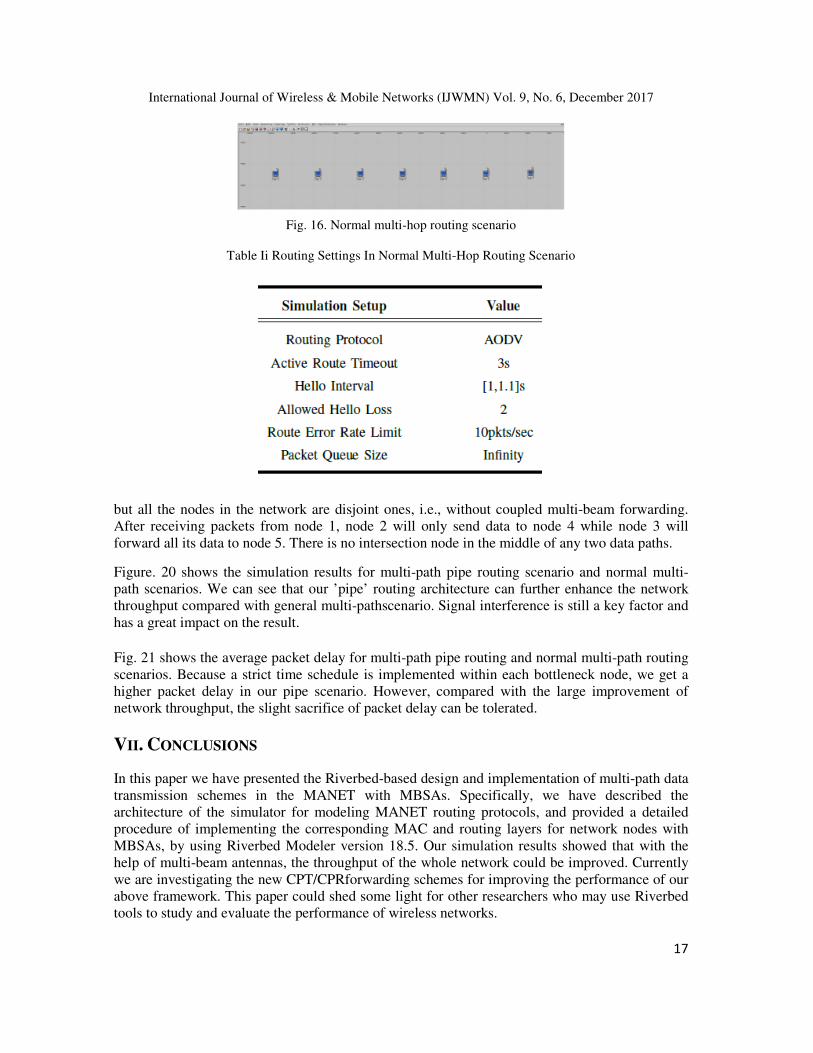
Fig. 14 shows the throughput of node 1. The throughput of node 6 is almost the same as node 1

since we use the same schedule in our CPT-CPR scenario. Based on the packet generation

settings we can see that each regular node sends 250 packets every second. From the figure we

can see that MBSA can significantly increase the throughput of the bottleneck nodes. Fig. 15

shows the average packet delay of node 1 in CPT-CPR scenario (the result of node 6 is also quite

similar).

For multi-hop diamond routing scenario, we compare it with a normal multi-hop routing scenario,

which is shown in Fig. 16. In normal multi-hop routing scenario, node 1 is the source node and

node 7 is the destination node. All the data packets will be forwarded through the same route.

Both multi-hop diamond routing and its control group have six hops in total. Table II shows the

selected routing settings for the normal multi-hop routing scenario.

Fig. 17 shows the network throughput for multi-hop diamond routing scenario as well as the

normal multi-hop forwarding scenario. Compared with normal multi-hop scenario, our diamond

routing scheme can achieve satisfactory through


16

Fig. 14. Throughput of node 1 in CPT-CPR scenario

Fig. 15. Packet Delay of node 1 in CPT-CPR scenario

put in the first two hops, but its throughput goes down as the number of the hops increases, which

is reasonable in multihop data relay case. Although the diamond routing scenario has three more

data links in every hop, local synchronization in bottleneck node needs certain communication

overhead. More hops in data transmission means longer time to synchronize the CPR and CPT

operations.

Fig. 18 shows the average packet delay for multi-hop diamond routing scenario and normal multi-

hop scenario. From the figure we can see that the delay of our proposed scenario is a little higher

than the compared one. There are three reasons for this. First, local synchronization is a time-

consuming process. Second, our routing layer has multi-neighbor address analysis and multi-

queue packet distribution tasks to perform, which also takes some time. Third, we need to put

more information (beam-id) into channel control packets. However, with the increase of hops, the

difference between those two scenarios becomes negligible.

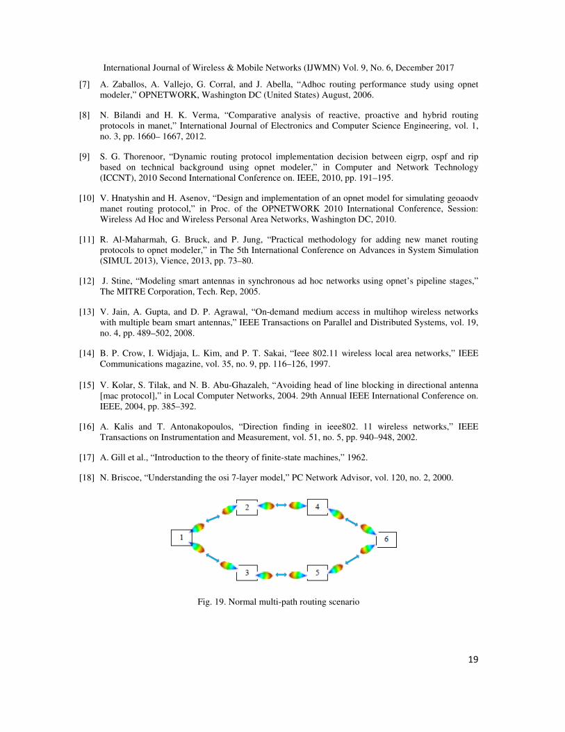
For multi-path pipe routing scenario, we compare it with a normal multi-path routing scenario,

which is shown in Fig. 19. In normal multi-path routing scenario, we also have 6 nodes,


17

Fig. 16. Normal multi-hop routing scenario

Table Ii Routing Settings In Normal Multi-Hop Routing Scenario

but all the nodes in the network are disjoint ones, i.e., without coupled multi-beam forwarding.

After receiving packets from node 1, node 2 will only send data to node 4 while node 3 will

forward all its data to node 5. There is no intersection node in the middle of any two data paths.

Figure. 20 shows the simulation results for multi-path pipe routing scenario and normal multi-

path scenarios. We can see that our ’pipe’ routing architecture can further enhance the network

throughput compared with general multi-pathscenario. Signal interference is still a key factor and

has a great impact on the result.

Fig. 21 shows the average packet delay for multi-path pipe routing and normal multi-path routing

scenarios. Because a strict time schedule is implemented within each bottleneck node, we get a

higher packet delay in our pipe scenario. However, compared with the large improvement of

network throughput, the slight sacrifice of packet delay can be tolerated.

VII. CONCLUSIONS

In this paper we have presented the Riverbed-based design and implementation of multi-path data

transmission schemes in the MANET with MBSAs. Specifically, we have described the

architecture of the simulator for modeling MANET routing protocols, and provided a detailed

procedure of implementing the corresponding MAC and routing layers for network nodes with

MBSAs, by using Riverbed Modeler version 18.5. Our simulation results showed that with the

help of multi-beam antennas, the throughput of the whole network could be improved. Currently

we are investigating the new CPT/CPRforwarding schemes for improving the performance of our

above framework. This paper could shed some light for other researchers who may use Riverbed

tools to study and evaluate the performance of wireless networks.


18

Fig. 17. Network throughput comparison between multi-hop diamond routing and normal multi-hop routing

Fig. 18. Packet delay comparison between multi-hop diamond routing and normal multi-hop routing

REFERENCES

[1] J. Macker, “Mobile ad hoc networking (manet): Routing protocol performance issues and evaluation

considerations,” 1999.

[2] E. M. Royer and C.-K. Toh, “A review of current routing protocols for ad hoc mobile wireless

networks,” IEEE personal communications, vol. 6, no. 2, pp. 46–55, 1999.

[3] C. E. Perkins et al., Ad hoc networking. Addison-wesley Reading, 2001, vol. 1.

[4] C. Perkins, E. Belding-Royer, and S. Das, “Ad hoc on-demand distance vector (aodv) routing,” Tech.

Rep., 2003.

[5] T. Clausen and P. Jacquet, “Optimized link state routing protocol (olsr),” Tech. Rep., 2003.

[6] O. Modeler, “Riverbed technology,” Inc. http://www. riverbed. com,

2016.


19

[7] A. Zaballos, A. Vallejo, G. Corral, and J. Abella, “Adhoc routing performance study using opnet

modeler,” OPNETWORK, Washington DC (United States) August, 2006.

[8] N. Bilandi and H. K. Verma, “Comparative analysis of reactive, proactive and hybrid routing

protocols in manet,” International Journal of Electronics and Computer Science Engineering, vol. 1,

no. 3, pp. 1660– 1667, 2012.

[9] S. G. Thorenoor, “Dynamic routing protocol implementation decision between eigrp, ospf and rip

based on technical background using opnet modeler,” in Computer and Network Technology

(ICCNT), 2010 Second International Conference on. IEEE, 2010, pp. 191–195.

[10] V. Hnatyshin and H. Asenov, “Design and implementation of an opnet model for simulating geoaodv

manet routing protocol,” in Proc. of the OPNETWORK 2010 International Conference, Session:

Wireless Ad Hoc and Wireless Personal Area Networks, Washington DC, 2010.

[11] R. Al-Maharmah, G. Bruck, and P. Jung, “Practical methodology for adding new manet routing

protocols to opnet modeler,” in The 5th International Conference on Advances in System Simulation

(SIMUL 2013), Vience, 2013, pp. 73–80.

[12] J. Stine, “Modeling smart antennas in synchronous ad hoc networks using opnet’s pipeline stages,”

The MITRE Corporation, Tech. Rep, 2005.

[13] V. Jain, A. Gupta, and D. P. Agrawal, “On-demand medium access in multihop wireless networks

with multiple beam smart antennas,” IEEE Transactions on Parallel and Distributed Systems, vol. 19,

no. 4, pp. 489–502, 2008.

[14] B. P. Crow, I. Widjaja, L. Kim, and P. T. Sakai, “Ieee 802.11 wireless local area networks,” IEEE

Communications magazine, vol. 35, no. 9, pp. 116–126, 1997.

[15] V. Kolar, S. Tilak, and N. B. Abu-Ghazaleh, “Avoiding head of line blocking in directional antenna

[mac protocol],” in Local Computer Networks, 2004. 29th Annual IEEE International Conference on.

IEEE, 2004, pp. 385–392.

[16] A. Kalis and T. Antonakopoulos, “Direction finding in ieee802. 11 wireless networks,” IEEE

Transactions on Instrumentation and Measurement, vol. 51, no. 5, pp. 940–948, 2002.

[17] A. Gill et al., “Introduction to the theory of finite-state machines,” 1962.

[18] N. Briscoe, “Understanding the osi 7-layer model,” PC Network Advisor, vol. 120, no. 2, 2000.

Fig. 19. Normal multi-path routing scenario


20

Fig. 20. Network throughput comparison between multi-path pipe routing and normal multi-path routing

Fig. 21. Packet delay comparison between multi-path pipe routing and normal multi-path routing

RIVERBED -BASED NETWORK MODELING FOR MULTI -BEAM CONCURRENT...

Documents

Transcript of RIVERBED -BASED NETWORK MODELING FOR MULTI -BEAM CONCURRENT...