RIsk Valuation in Equity and Interest Rates Risk Factors
85
Risk Measures and Valuation under Interest Rates and Equity Risk Factors by Shu Pei Chew Department of Mathematics King’s College London The Strand, London WC2R 2LS United Kingdom Email: Shu [email protected] Tel: +44 (0)754 990 9234 4 September 2014 Report submitted in p ar tial fulfillment of the requirements for the degree of MSc in Financial Mathema tics in the University of London
-
Upload
chewshupei -
Category
Documents
-
view
219 -
download
0
Transcript of RIsk Valuation in Equity and Interest Rates Risk Factors

8/10/2019 RIsk Valuation in Equity and Interest Rates Risk Factors
http://slidepdf.com/reader/full/risk-valuation-in-equity-and-interest-rates-risk-factors 1/85
Risk Measures and Valuation underInterest Rates and Equity Risk Factors
by
Shu Pei Chew
Department of MathematicsKing’s College London
The Strand, London WC2R 2LSUnited Kingdom
Email: Shu [email protected]: +44 (0)754 990 9234
4 September 2014
Report submitted in partial fulfillment of
the requirements for the degree of MSc in
Financial Mathematics in the University of
London

8/10/2019 RIsk Valuation in Equity and Interest Rates Risk Factors
http://slidepdf.com/reader/full/risk-valuation-in-equity-and-interest-rates-risk-factors 2/85
Abstract
The financial disasters that occurred in the early 1990s clearly portray lack
of knowledge on the various risk valuation approaches. Market risks suchas equity risk and interest risk often pose threat and uncertainty to portfo-lio investment strategies. This paper examines the different risk valuationapproaches. More specifically, we will study the concepts of Value at Risk(VaR) and Expected Shortfall (ES). We employ delta-normal, delta-gammaand Monte Carlo methods to measure VaR, as well as ES. Whilst comparingthe methods, we run the numerical test by proposing two different portfolios.The portfolios are constructed in such a way that one consist of equity riskand the other is made up of both equity and interest rate risk. As such,we introduce the classic Black-Scholes model for equity risk and the Vasicek
model for interest rate risk. Since estimation contributes to risk valuation, wefurther discuss the problems encountered when using statistical estimationlike the Maximum Likelihood Estimator.
1

8/10/2019 RIsk Valuation in Equity and Interest Rates Risk Factors
http://slidepdf.com/reader/full/risk-valuation-in-equity-and-interest-rates-risk-factors 3/85
8/10/2019 RIsk Valuation in Equity and Interest Rates Risk Factors
http://slidepdf.com/reader/full/risk-valuation-in-equity-and-interest-rates-risk-factors 4/85
Contents
1 INTRODUCTION 5
2 LITERATURE REVIEW 8
2.1 The Black and Scholes Model: Assumptions . . . . . . . . . . 8
2.1.1 Risk Factors . . . . . . . . . . . . . . . . . . . . . . . . 9
2.2 The Interest Rate Model . . . . . . . . . . . . . . . . . . . . . 10
2.2.1 The Vasicek Model (1997) . . . . . . . . . . . . . . . . 11
2.3 Pricing of Options . . . . . . . . . . . . . . . . . . . . . . . . 14
2.4 The Greeks . . . . . . . . . . . . . . . . . . . . . . . . . . . . 16
2.4.1 Delta, δ . . . . . . . . . . . . . . . . . . . . . . . . . . 16
2.4.2 Gamma, Γ . . . . . . . . . . . . . . . . . . . . . . . . . 17
2.5 Risk Measurement . . . . . . . . . . . . . . . . . . . . . . . . 18
2.5.1 Value-at-Risk, VaR . . . . . . . . . . . . . . . . . . . . 18
2.5.2 Expected Shortfall, ES . . . . . . . . . . . . . . . . . . 22
2.6 Standard Methods . . . . . . . . . . . . . . . . . . . . . . . . 242.6.1 Delta Approximation . . . . . . . . . . . . . . . . . . . 24
2.6.2 Delta-Gamma Approximation . . . . . . . . . . . . . . 27
2.6.3 Monte Carlo Simulation . . . . . . . . . . . . . . . . . 29
3 NUMERICAL ANALYSIS 32
3.1 Outline . . . . . . . . . . . . . . . . . . . . . . . . . . . . . . . 32
3

8/10/2019 RIsk Valuation in Equity and Interest Rates Risk Factors
http://slidepdf.com/reader/full/risk-valuation-in-equity-and-interest-rates-risk-factors 5/85
3.2 Methodology . . . . . . . . . . . . . . . . . . . . . . . . . . . 33
3.3 Results . . . . . . . . . . . . . . . . . . . . . . . . . . . . . . . 43
3.4 Discussion . . . . . . . . . . . . . . . . . . . . . . . . . . . . . 45
4 ESTIMATION 49
4.1 Estimation . . . . . . . . . . . . . . . . . . . . . . . . . . . . . 50
4.1.1 Maximum Likelihood . . . . . . . . . . . . . . . . . . . 50
4.1.2 Maximum Likelihood of Black Scholes Model for Stock
Price . . . . . . . . . . . . . . . . . . . . . . . . . . . . 514.1.3 Maximum Likelihood of Vasicek Model for Short Rates 52
4.2 Calibration . . . . . . . . . . . . . . . . . . . . . . . . . . . . 55
4.2.1 Calibration of Black Scholes Option Price . . . . . . . 55
4.2.2 Calibration of Vasicek Model for Yield Using MLE . . 55
4.3 Empirical Analysis . . . . . . . . . . . . . . . . . . . . . . . . 57
4.3.1 MLE Test for Geometric Brownian motion and VasicekModel for Short Rate . . . . . . . . . . . . . . . . . . . 57
4.3.2 Estimation using Raw Data . . . . . . . . . . . . . . . 58
4.4 Discussion . . . . . . . . . . . . . . . . . . . . . . . . . . . . . 61
5 CONCLUSION 63
6 APPENDIX 65
6.1 Matlab Code for Chapter 3 . . . . . . . . . . . . . . . . . . . 65
6.1.1 Delta Normal . . . . . . . . . . . . . . . . . . . . . . . 686.1.2 Delta-Gamma . . . . . . . . . . . . . . . . . . . . . . . 70
6.1.3 Monte Carlo VaR . . . . . . . . . . . . . . . . . . . . . 73
6.1.4 Monte Carlo ES . . . . . . . . . . . . . . . . . . . . . . 74
6.2 Matlab Code for Chapter 4 . . . . . . . . . . . . . . . . . . . 76
4

8/10/2019 RIsk Valuation in Equity and Interest Rates Risk Factors
http://slidepdf.com/reader/full/risk-valuation-in-equity-and-interest-rates-risk-factors 6/85
Chapter 1
INTRODUCTION
The market and financial instability is the main reason why risk measure-ment continues to evolve in the past decade. The highly volatile environ-ment has caused rapid development in the risk management field. Financialrisk consists of market risk, credit risk, liquidity risk and so on. The studyof risk management has drawn attention of many intellectuals from differ-ent disciplines. The theory and practice of risk management have evolvedcontinuously since the work of Markowitz in modern portfolio theory, as in
[1]. Followed by Sharpes capital asset pricing model in [2], which examinesrelationship between rates of return of efficient portfolio with its standarddeviation. In 1997, the Nobel Prize in Economics was awarded to Black andScholes for their pioneering work in publishing the paper, The Pricing of Options and Corporate Liabilities. The Black Scholes model, established byBlack and Scholes in [3] remains one of the most fundamental mathematicalmodels used to estimate the price of European-style options.
The risk measure that most financial institutions favor is Value at Risk(VaR). The aim of the development of VaR is to manage global market risk.In the early 1990s, financial institutions were threatened by losses attributed
by derivatives as interest rates became more volatile. The financial disasterssuch as the Barings PLC (1995), Metallgesellschaft (1993), Orange County(1994), Daiwa (1995) and so on, have led to increasing concerns with regard tothe risk measure approach. For example, the Orange County affair perfectlyportrays the effect of the lack of control over market risk measurements.Jorion made the comment in [5], ” It is fair to surmise that had the VaRbeen made public, investors probably would have been more careful with theirfunds ”. In relation to Jorions comment, I do believe that VaR would haveincreased risk transparency and thereby helping reduce risk exposure. After
5

8/10/2019 RIsk Valuation in Equity and Interest Rates Risk Factors
http://slidepdf.com/reader/full/risk-valuation-in-equity-and-interest-rates-risk-factors 7/85
the crisis, it became apparent that the knowledge of adapting VaR approach
is highly essential as it, in general, provides estimates of future losses byhistorical or present data. Thus, the Chairman of JP Morgan developedRiskMetrics system and presented in [11], such that the system incorporatesVaR measure based on portfolio theory. The RiskMetrics approach involvesidentifying underlying risk factors, estimating volatilities and correlations,computing systems (Monte Carlo simulations) with scenario analysis.
Despite its usefulness, VaR also has its drawbacks and has been heav-ily criticized by many in various ways. In 1997, Artzner, Delbaen, Ebberand Heath published a paper, ” Thinking Coherently ” in [6], where theyexplained that risk measures should satisfy coherence property that is clas-sified by four axioms. VaR did not satisfy the subadditivity property and soit is not a coherent risk measure. Acerbi, Nordio and Sirtori succeeded inconstructing a coherent risk measure in paper [31], where they have intro-duced Expected Shortfall (ES) as a fundamental tool in risk management.The 2008 crisis greatly exposed the weakness in the capital treatment of trading activities and led the Basel Committee on Banking Supervision toturn attention towards the trading book. In July 2009, the Basel Committeepresented a set of revisions to Basel II and later on initiated a fundamentalreview of trading book. From [8], we know that the lack of coherence in riskmeasures was insufficient to maintain the banks resource. Thus, the com-
mittee suggested that the VaR to be replaced by ES. This helped implementcapital requirements for specific risk factors and thereby strengthening bank-ing regulatory standards. Financial institutions favor ES over VaR becauseit takes into consideration losses beyond VaR value.
The structure of this paper is:
Chapter 1: We will start off with some literature on the Black Scholesmodel and risk factors. In this paper, the short-term interest rate modelthat we will be using is the Vasicek model. We then use the Black Scholesand Vasicek model to derive prices of equity options under both deterministic
and stochastic interest rate. The next part of this chapter focuses on present-ing formal definitions of VaR, ES and coherence property. There are manyapproaches used to calculate VaR and ES. We will discuss three differentmethods to calculate risk measures.
Chapter 2: I propose two different portfolios. The first portfolio isassumed to not represent a risk factor while the second portfolio is madeup of both equity and interest rate risk. We will compare the different riskmeasure calculation methods and also examine the dependence effect of thetwo risk factors on the results. Here, we will also discuss the pitfalls and
6

8/10/2019 RIsk Valuation in Equity and Interest Rates Risk Factors
http://slidepdf.com/reader/full/risk-valuation-in-equity-and-interest-rates-risk-factors 8/85
merits of the methods.
Chapter 3: We will shed light on the importance of estimation andcalibration of models in risk management. As such, we introduce MaximumLikelihood estimation and calibration of Vasicek and Black Scholes model.Lastly, we run tests on maximum likelihood estimator with simulated dataand market data to observe the bias between estimate and estimator. Wefurther examine estimation by applying it to market data.
7

8/10/2019 RIsk Valuation in Equity and Interest Rates Risk Factors
http://slidepdf.com/reader/full/risk-valuation-in-equity-and-interest-rates-risk-factors 9/85
Chapter 2
LITERATURE REVIEW
The first step in analyzing risk is to identify the pricing model that evaluatesthe value of the derivative with respect to underlying risk factors. In our case,we will discuss the valuation of the Black-Scholes option pricing model by firstpresenting some standard theory of underlying risk factors and associatedstochastic models (e.g., the Vasicek model). Then we implement in detailthe different approaches used to estimate VaR and ES.
2.1 The Black and Scholes Model: Assump-tions
An option is a contract agreed upon by two parties, the buyer and seller.This gives the owner the right, but not the obligation to buy or sell theunderlying asset. A Call option gives the owner the right to buy the asset,whereas a put option gives the owner the right to sell the asset. Moreover,there are different styles of options. In this paper, we will focus on European
options, giving the investor the right to exercise the share of the stock onlyat maturity date, T. The Black Scholes formula has been highly popularizeddue to it’s ability to model price of options. Also, by taking the first partialdifferentiation of the Black Scholes formula, one can create a delta-neutralportfolio in the sense that it is insensitive to changes of stock price. Paperspublished by Black-Schoes in [3] and Merton in [10] emphasized on valuingoptions on stocks, and their findings eventually became one of the mostimportant concepts in finance. In the process of deriving the Black Scholesequation, the following assumptions on the market are made:
8

8/10/2019 RIsk Valuation in Equity and Interest Rates Risk Factors
http://slidepdf.com/reader/full/risk-valuation-in-equity-and-interest-rates-risk-factors 10/85
1. The short-term interest rate, r is known and constant.
2. Under geometric brownian motion assumptions, the dynamic of thestock price process satisfies the stochastic differential equation (SDE):
dS t = µS tdt + σsS td W t, under P measure, (2.1)
where S t is the stock price at time t, σs is the volatility, µ is the driftterm and W t is the brownian motion under P measure.
dS t = rS tdt + σsS tdW t, under Q measure, (2.2)
whereas in equation (2.2), by using Girsanov Theorem and the changeof measure, the brownian motion W t is under Q measure1. The Brow-nian motions are both normally distributed, W t, W t ∼ N (0, t)
3. The stock pays no dividend.
4. The market is ”frictionless”, indicating that there is no transactioncosts.
As any financial model, one can proceed to the ”core” when the as-sumptions are satisfied. In our context, it would be the evaluation of theBlack-Scholes pricing model for European options, which will be discussedin section 2.3.
2.1.1 Risk Factors
Identifying risk factors, affecting your position, are essential as it allows usto compute the value of the security. For example, given an equity option,the corresponding risk factor would be the price of the equity or impliedvolatility. As for a bond, the risk factor would be the interest rate.The general setting of the model is in a probability space (Ω , F, (F t)0≤t,P).
1The risk neutral measure, Q, is said to be equivalent to the real probability measure,P, by using the Girsanov theorem. This changes the Brownian motion by adding a drift.To review more details on I.V.Girsanov’s work, see [12]
9

8/10/2019 RIsk Valuation in Equity and Interest Rates Risk Factors
http://slidepdf.com/reader/full/risk-valuation-in-equity-and-interest-rates-risk-factors 11/85

8/10/2019 RIsk Valuation in Equity and Interest Rates Risk Factors
http://slidepdf.com/reader/full/risk-valuation-in-equity-and-interest-rates-risk-factors 12/85
and Scholes model in section 2.1, has provided an enormous contribution to
the finance world. We relax the assumption that the interest rate is constant,thus allowing it to be stochastic as it poses as another risk factor. This meansthat interest rate takes the form of a random variable where its movementsare elastic around trends.
Despite the vast research, modeling interest rates remain challengingdue to the existence of term-structure. Term structure of interest rate, oftenbeing referred to as yield curve, describes the relationship between interestrate on zero-coupon bonds and its maturities. From a financial risk modelingstandpoint, dynamics of the interest rate is important in determining futureinterest rate levels given the unpredictable nature of the term structure of interest rates. Moreover, proper knowledge of the term structure enables usto derive zero-coupon bond price. In relation to that, Duffie and Kan in[13] presented a set of models classified as affine term structure models andexamined it, numerically, by calculating prices of term-structure derivatives.Typically, the models that fall into this affine class are models of Vasicek in[9], Dothan in [14], Ho and Lee in [15] and many others. In this paper, for-mal understanding of the interest rate model, more specifically the Vasicekmodel, is a prerequisite for calculation of risks.
2.2.1 The Vasicek Model (1997)
First, let us consider the general dynamics of the short rate (rt)t≥0, as de-scribed in [17], in the risk neutral measure Q
dr(t) = b(t, r(t))dt + σ(t, r(t))dZ t, (2.7)
where b(t, rt) and σ(t, rt) are deterministic functions, which represent thedrift and diffusion of the process (rt)t
≥0, with Z t being a Brownian motion
under Q. Time-homogeneous models are ones that assume that the dynamicsof short rates depend on a constant coefficient, where short rates evolve withtime. An example of a time-homogeneous model is the Vasicek model,
dr(t) = kr(θ − r(t))dt + σrdZ t, r(0) = r0 (2.8)
where kr, θ and σr are constants. In [9], Vasicek described the term kr(θ −r(t)) as the instantaneous drift which pulls the process towards its mean term,θ. Equation (2.8) is a form of equation (2.7) where b(t, r(t)) = kr(θ − r(t))
11

8/10/2019 RIsk Valuation in Equity and Interest Rates Risk Factors
http://slidepdf.com/reader/full/risk-valuation-in-equity-and-interest-rates-risk-factors 13/85
and σ(t, r(t)) = σr. Multiplying (2.8) by ekrt and integrating it will give us
the solution for the SDE,
ekrtdr(t) + ekrtkrr(t)dt = krθekrtdt + ekrtσrdZ t
d(ekrtr(t)) = kθekrtdt + ekrtσrdZ t, ts
d(ekrur(u)) =
ts
krθekru du +
ts
ekruσr dZ u,
ekrtr(t) = ekrtr(s) + θekrt − θekrs +
ts
ekruσr dZ u,
r(t) = r(s)e−kr(t−s) + θ(1 − e−kr(t−s)) + σr
t
s
e−kr(t−u) dZ u (2.9)
(rt)t≥0 is Gaussian with mean and variance,
E[r(t)|F s] = E[r(s)e−kr(t−s) + θ(1 − e−kr(t−s)) + σr
ts
e−kr(t−u) dZ u|F s]
= r(s)e−kr(t−s) + θ(1 − e−kr(t−s)),
V ar[r(t)|F (s)] = σ2r e−krtV ar[
t
s
ekru dZ u
= σ2
r
2kr
[1 − e−2kr(t−s)]
As mentioned above that the Vasicek model is an affine term-structure inter-est rate model, thus the price of a zero-coupon bond P(t,T) can be determinedeasily. We let P(t,T) be the price of the zero-coupon bond at time t, matur-ing at time T, T ≥ t. The maturing value isP (T, T ) = 1, where the financialinstrument pays it’s holder 1 unit of cash at maturity time T. P(t,T) can beexpressed as the following
P (t, T ) = e−A(t)
−B(t)r(t)
(2.10)
where A(t) and B(t) satisfiesdA(t)
dt = 1
2σ2
r B(t) − krθB(t), A(T ) = 0dB(t)
dt = krB(t) − 1, B(T ) = 0
(2.11)
12

8/10/2019 RIsk Valuation in Equity and Interest Rates Risk Factors
http://slidepdf.com/reader/full/risk-valuation-in-equity-and-interest-rates-risk-factors 14/85
First, we solve for B(t)
e−krt(dB(t)
dt − krB(t)) = −e−krt
T
t
d(e−kruB(u)) =
T
t
−e−kru du
B(t) = 1
kr
(1 − e−kr(T −t))
We use the solution of B(t) to obtain A(t)
dA(t)dt
= 12
σ2r B(t) − krθB(t)
A(t) =
T
t
krθB(s) − 1
2σ2B(s)2 ds
A(t) = θ
kr
(e−kr(T −t) + kr(T − t) − 1)
− σ2
4k3r
(2kr(T − t) + 4e−kr(T −t) − e−2kr(T −t) − 3)
Finally, we combine the results of A(t), B(t) and equation (2.10). This follows
from [19]
⇒ P (t, T ) = e(− θ
kr (e−kr(T −t)+kr(T −t)−1)+ σ2
4k3r(2kr(T −t)+4e−kr(T −t)−e−2kr(T −t)−3))
e− 1kr (1−e−kr(T −t))r(t)
(2.12)
Based on the Heath-Jarrow-Morton methodology by Heath, Jarrow and Mor-ton in [18], one can formulate the general instantaneous forward rate, f(t,T)and also express forward rate, f(t,T), in terms of zero-coupon price, P(t,T)
df (t, T ) = α(t, T )dt + σ(t, T )dZ t, in the P measure (2.13)
f (t, T ) = − ∂
∂T log P (t, T ) (2.14)
where α(t, T ) and σ(t, T ) are progressively measurable processes. By usingfundamental theorem of calculus and Ito’s formula on (2.14), we can deducethat the price of zero-coupon bond satisfies
dP (t, T )
P (t, T ) = (r(t) + α∗(t, T ) +
1
2|σ∗(t, T )|2)dt + σ ∗ (t, T )dZ t (2.15)
13

8/10/2019 RIsk Valuation in Equity and Interest Rates Risk Factors
http://slidepdf.com/reader/full/risk-valuation-in-equity-and-interest-rates-risk-factors 15/85
where α∗(t, T ) =
− T
t α(t, u) du and σ∗(t, T ) =
− T
t σ(t, u) du. Thus, the
instantaneous forward rate for the Vasicek model can be obtained from ap-plying Ito to equation (2.14)
df (t, T ) = [σ2
r
k (e−kr(T −t) − e−2kr(T −t)) + σrθe−kr(T −t)]dt + σre−kr(T −t)dZ t
(2.16)
where α(t, T ) = σ2r
k (e−kr(T −t)−e−2kr(T −t))+σrθe−kr(T −t) and σ(t, T ) = σre−kr(T −t).
Next we substitute α∗(t, T ) and σ∗(t, T ) into (2.15), such that the price of
zero coupon bond satisfies
dP (t, T )
P (t, T ) = [r(t) −
T
t
[σ2
r
kr
(e−kr(T −t) − e−2kr(T −t)) − σrθe−kr(T −t)]dt
+ 1
2| T
t
σre−kr(T −t) dt|2]dt − (
T
t
σre−kr(T −t) dt)dZ t
= [r(t) + σrθ
kr
(e−kr(T −t) − 1)]dt + σr
kr
(e−kr(T −t) − 1)dZ t
(2.17)
2.3 Pricing of Options
In the Black-Scholes setting (section 2.1), we can calculate the price of theEuropean option by discounting and taking the expectation of the optionpayoff, under the risk neutral measure Q,
EQ payof f
B(t)
B(T )|F t
where we denote B(t) = e
t
0
rs ds
as the bank account.
• Call and Put Option Price with Deterministic Interest Rate, r
For a call option payoff at time t, H c, if the stock price,S T , is higherthan the exercise price, K, then the value of the option equals to thestock price minus the exercise price (S T − K ). On the other hand, if the stock price, S T , is less than the exercise price, K, then the valuewill be zero. Thus, the call option payoff is H c = (S T −K )+. Whereas,the payoff of the put option is H p = (K − S T )
+. We now have all the
14

8/10/2019 RIsk Valuation in Equity and Interest Rates Risk Factors
http://slidepdf.com/reader/full/risk-valuation-in-equity-and-interest-rates-risk-factors 16/85
ingredients to formulate our option prices on stock, S. First, the Call
C t and Put P t option prices at time t with constant interest rate r,which follows from [22],
C t = EQ
(S T − K )+
B (t)
B(T )|F t
= S tN (d1) − Ke−r(T −t)N (d2), (2.18)
P t = EQ
(K − S T )
+ B (t)
B(T )|F t
= K e−r(T −t)N (−d2) − S tN (−d1),
(2.19)
d2 = log S t
K + (r − σ2s
2 )(T − t)
σs
√ T − t
(2.20)
d1 = log S t
K + (r + σ2
s
2 )(T − t)
σs
√ T − t
(2.21)
where N ( ) is the cumulative function of the standard normal, (T − t)is the time to maturity and σs is the volatility of returns of stock.
• Call Option Price with Stochastic Interest Rate, rt
The next derivation we are interested in is the value of an at-the-money(ATM) call option under Vasicek interest rate model. A call option thatis ATM if the current stock, S t equals to the strike price, K, S t = K .The European option price under Hull and White process (1994) hasbeen previously reviewed by Brigo and Mercusio in [17]. The Hull-White model, also known as the Extended Vasicek model, as beingdefined in [20] is
dr(t) = (θ(t) − K rr(t))dt + σrdZ t
where, θ(t) is deterministic. It is essentially the Vasicek model when
θ(t) is a constant, more specifically θ(t) = krθ. It follows from [17] thatthe ATM (S 0 = K ) European call option price at time t, using Vasicekmodel introduced in section 2.2.1, is of the following,
C atm;t = P (t, T )EQT
[(S T − K )+|F t] (2.22)
= S (t)N (a1) − KP (t, T )N (a2) (2.23)
15

8/10/2019 RIsk Valuation in Equity and Interest Rates Risk Factors
http://slidepdf.com/reader/full/risk-valuation-in-equity-and-interest-rates-risk-factors 17/85

8/10/2019 RIsk Valuation in Equity and Interest Rates Risk Factors
http://slidepdf.com/reader/full/risk-valuation-in-equity-and-interest-rates-risk-factors 18/85
Delta is sensitive to market changes where a unit change in option price
results in unit change in stock price. Besides allowing financial traders tohedge option risk, delta provides a numerical exposure to nonprofessionalsat no cost. However, Taleb criticized in [21] that the significance of deltaapproach to risk managing is limited to simple options, where performs asan extremely weak measure when we consider long or short options. Despiteits shortcomings, delta is still widely used by traders but with caution. Deltafor various types of options with respect to S t are:
1. The general formula for the delta of an Option: δ = ∂C ∂S
2. Delta of a Call Option: δ call = N (d1)3. Delta of a Put Option: δ put = −N (−d1) = N (d1) − 1
4. Delta of a ATM Call Option: δ s = ∂C atm;t
∂S t= N (a1)
where a1 = log
StKP (t,T )+
12v2(t,T )
v(t,T ) and d1 =
log StK +(r+
σ2s2 )(T −t)
σs√
T −t .
2.4.2 Gamma, Γ
A portfolio is gamma hedged such that it’s value will be insensitive to secondorder changes to stock price. The gamma (Γ) of an option refers to the rateof change of portfolio’s delta with respect to asset. Mathematically, it isthe second derivative of price of derivative (option) to asset (stock) price, asfollows from [22].
1. The general representation for gamma of an Option: Γ = ∂ 2C ∂S
2. Gamma of a Call and Put Option:Γcall = Γ put = N (d1)
σsS t√
T −t
Γcall = Γ put = 1√ 2π e−(d1)2 12 ∂d1
∂S = 1√ 2π [ S te
r(T
−t)
K ]−12 e−y[ K S tσs
√ T − t ]
3. Gamma of a ATM Call Option: Γs = ∂ 2C atm,t
∂S 2t= N (a1)
v(t,T )S t
where y = (log
StK
er(T −t))2+ 14σ2
s(T −t)2
2σ2s(T −t)
. On a gamma to stock price graph, thegamma of a stock option increases as the stock price increases to the strikeprice, K. Also, Taleb in [21] mentioned that for an ATM call option, thegamma is maximum when option nears expiration.
17

8/10/2019 RIsk Valuation in Equity and Interest Rates Risk Factors
http://slidepdf.com/reader/full/risk-valuation-in-equity-and-interest-rates-risk-factors 19/85
2.5 Risk Measurement
A risk is defined as the likelihood of occurrence of a bad consequence oreffect on a position, often associated with a probability. Typically, onlythe downside of risk is being discussed by risk managers. As such, riskmeasurements are designed to address this matter. In this section, we willexplore value-at-risk (VaR), a highly recognized risk measure discussed inBasel II capital adequacy framework, and examine VaR from the view of coherence risk measure. Also, we will review the mathematical concepts of expected shortfall (ES) whilst highlighting the differences between VaR andES risk measures.
2.5.1 Value-at-Risk, VaR
A portfolio is composed of many risk factors and often not easy to manage.VaR provides a consistent measure of risk where its methodology has beenextended towards measuring credit risks, where the probability of default of a financial institution is taken into account. Numerical information can beused for optimizing purposes as risk managers aim to minimize VaR such thatthey can assess risk better, improving investment strategies. More formally,
VaR measures the maximum potential loss of financial instruments-tradeablepackages of capital that has a monetary value- with a given confidence levelover a horizon of time period. An investor may ask the question: What ismy maximum loss in α% best case of portfolio over a targeted horizon. Theanswer to the question lies within the definition of VaR.
Definition 2.5.1. (Value-at-Risk) It follows from [23], given some confi-dence level α ∈ (0, 1). A d-day VaR of a portfolio, V aRα at confidence level α is defined as the smallest value of x such that the probability of maximum loss X that takes value less than x is greater that α.
x(α) = F −1(α) = inf
x : F (x) > α
(2.24)
= inf x : P(X ≤ x) > α) (2.25)
where equation (2.24) is the α-quantile of F (x). VaR can be written as
V aRα = −x(α) = −inf x : P(X > x) ≤ 1 − α),
where P(X > x) denotes the probability of loss, X, exceeds x. Quantiles are closely related to VaR in probabilistic terms, in the sense that xα is the α-quantile of a cumulative distribution function F (x) of the profit and loss distribution.
18
8/10/2019 RIsk Valuation in Equity and Interest Rates Risk Factors
http://slidepdf.com/reader/full/risk-valuation-in-equity-and-interest-rates-risk-factors 20/85
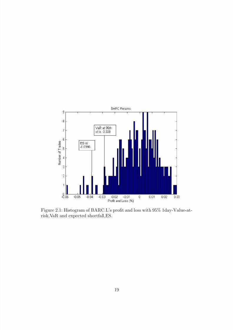
Figure 2.1: Histogram of BARC.L’s profit and loss with 95% 1day-Value-at-risk,VaR and expected shortfall,ES.
19

8/10/2019 RIsk Valuation in Equity and Interest Rates Risk Factors
http://slidepdf.com/reader/full/risk-valuation-in-equity-and-interest-rates-risk-factors 21/85
Proposition 2.5.2. With reference to [23], the loss distribution P(X
≤x) =
F x is strictly increasing and X is normally distributed, X ∼ N (µ, σ2), and α ∈ (0, 1) such that we have
F x(−V aRα) = α (2.26)
We introduce an alternative expression for VaR
V aRα = −µ − σF −1(α)
The proof of proposition 2.5.2:
P(X ≤ −V aRα) = P(
X
−µ
σ ≤ F −1
(α)) = P(Z ≤ F −1
(α)) = F (F −1
(α)) = α
where Z is standard normally distributed and F −1(α) is the ordinary inverseof F.
The essential parameters to be considered when dealing with VaR calcu-lations are holding period, d and confidence level, α. Typically, risk managersfavor taking confidence level of 90%, 95% and 99%. In practice, the Baselcommittee requires banks to derive 10day-VaR at a 99 % confidence level ,one-tailed confidence interval, to ensure risks that are embedded at the tailcan be captured accurately.
To help illustrate the notion of VaR, we have collected a set of data.The data consists of daily simulated returns of BARC.L with a total of 270observations that were obtained from the Bloomberg. Figure 2.1 representsthe histogram of BARC.L’s simulated profit and loss with α = 95% 1 day-VaR and ES, under the assumption (section2.1) that it follows log returnson stock. The 95% 1 day-VaR is approximately V aRα = 0.028, indicatingthat the probability of loss exceeding this amount is less than 5%. The valueat the extreme left of the histogram indicates the maximum loss (or extremeoutlier) of BARC.L. We can concentrate on this behavior by using the ex-treme value theory technique (EVT) as in [26], which we will not be focusing
on in this paper. Note that ES takes into account the tail of the distribution,giving us a greater loss value.
One of the most crucial shortcomings of VaR is the fact that it fails tobe a coherent risk measure. Ever since the argument made by Artzner in[30], the non-subadditivity characteristic of VaR has been heavily criticizedby many risk professionals and researchers like Acerbi and Tasche in [28] and[29]. To avoid confusion, it is best to grasp a good understanding of theconcept of coherent risk measures, which brings us to our next definition.
20

8/10/2019 RIsk Valuation in Equity and Interest Rates Risk Factors
http://slidepdf.com/reader/full/risk-valuation-in-equity-and-interest-rates-risk-factors 22/85
Definition 2.5.3. (Coherent Risk Measure) As in [6] and[30], we consider
a set of random variables, A on probability space (Ω, F ,P). A risk measure ρ(X ) maps a random variable to a real number, R, meaning ρ : A → R for all X ∈ A. ρ(X ) can take both positive and negative values, where
ρ(X ) =
Positive value , represents the least extra cash to be added into X
Negative value , represents the amount of cash to be withdrawn from X
The expression ”cash” refers to an increase of equity into position X such that the information, ρ(X ) may lower the state of owing money in the balance sheet. A risk measure is coherent if it satisfies the following axioms:
1. Translation invariant : X ∈ A, a ∈ R ⇒ ρ(X + a) = ρ(X ) − aThis means that adding amount a cash into position will decrease the risk measure ρ(X ) by a.
2. Subadditivity : ∀ X 1, X 2 ∈ A ⇒ ρ(X 1 + X 2) ≤ ρ(X 1) + ρ(X 2)This means that the sum of two risk measure of different positions,ρ(X 1)+ρ(X 2) is greater or equal that risk measure of combined positions ρ(X 1 + X 2)
3. Positive homogeneity: for all α
≥0 and X
∈A,
⇒ ρ(αX ) = αρ(X )
Doubling the position,α has direct impact on the risk measure where it doubles by α.
4. Monotonicity: for X and Y ∈ A, st.X ≤ Y, ⇒ ρ(X ) ≥ ρ(Y )Position Y is more positive than X in the sense that it will be less risky.
Combination of axioms 2 (subadditivity) and 3 (positive homogeneity)results in the notion of convexity, which was introduced by Follmer and Schiedin [32]. As seen in [28], we know that VaR is not a coherent risk measuresince it does not satisfy the subadditivity characteristic. An example of the
non-subadditivity behavior of VaR has been illustrated nicely by Artzner,Delbaen, Eber and Heath,
” For a second example of non-subadditivity, briefly allow an infi-nite set Ω and consider two independent identically distributed randomvariables X 1 and X 2 having the same density 0.90 on the interval[0, 1],the same density 0.05 on the interval [2, 0]. Assume that each of themrepresents a future random net worth with positive expected value, that
21

8/10/2019 RIsk Valuation in Equity and Interest Rates Risk Factors
http://slidepdf.com/reader/full/risk-valuation-in-equity-and-interest-rates-risk-factors 23/85
is a possibly interesting risk. Yet, in terms of quantiles, the 10% valuesat risk of X 1 and X 2 being equal to 0, whereas an easy calculation show-ing that the 10% value at risk of X 1 + X 2 is certainly larger than 0, weconclude that the individual controls of these risks do not allow directlya control of their sum, if we were to use the 10% value at risk.”
Coherent Measures of Risk, (July 22, 1998) p . 14 [30]
Also, VaR discourages diversification as it fails to take into accounteconomic consequences in risk measurement. To summarize, due to VaR’sinability to follow subadditivity and capture tail or fat-tailed2 risk accurately,most risk practitioners turned attention towards ES, which will be our focusin the next section.
2.5.2 Expected Shortfall, ES
The popularized ES framework is a class of coherent risk measure, studiedin [28], which calculates the conditional loss in a position beyond VaR as
shown earlier in figure 2.1. In 2002, ES has been proven to have the sameform as Conditional Value-at-Risk (CVaR) by Rockafellar and Uryasev in[33]. Hence, a common term for ES is CVaR risk measure. Besides that,Rockafellar and Uryasev in [34] demonstrated optimization of CVaR andcalculation of VaR at the same time to further improve portfolio investmentdecisions. Many researches have studied ES as an alternative risk measureto VaR where they have proposed different methods of deriving ES. Theorder statistics approach was initiated by Acerbi and Tasche in [28] and hasbeen reviewed in many literatures since. Another direct method is by takingpartial derivatives of α-quantile to obtain mathematical formulation of ES,
as seen in [35].Reviewing our notations in def 2.5.1, We note that x(α) = inf x : F (x) > αas the upper α-quantile of X and VaR as V aRα = −x(α).
Definition 2.5.4. (Expected Shortfall, ES) (cf. definition 2 in [28] ) We
2Most financial data are fat-tailed, which tells us that the gain and losses, both endsof tail, are much higher in probability compares to Gaussian (Normal) distributions.
22

8/10/2019 RIsk Valuation in Equity and Interest Rates Risk Factors
http://slidepdf.com/reader/full/risk-valuation-in-equity-and-interest-rates-risk-factors 24/85
assume that E[X −] <
∞. First, defining the α-tail mean,
xα = 1
α(E[X X ≤x(α)] + x(α)(α − P[X ≤ x(α)])) (2.27)
= 1
α(E[X X ≤x(α)] + x(α)(α − E[ X ≤x(α)])) and we have ES,
(2.28)
ES α = −xα (2.29)
where is known as the indicator function such that,
X
≤x(α)
= 1, if X ≤ x(α)
0, otherwise
This means that if it does not satisfy the condition, X ≤ x(α), thenequation (2.29) will be equivalent to VaR such that ES α = V aRα
Proposition 2.5.5. As in [23] and [28], the loss distribution P(X ≤ x) =F x is strictly increasing and X is normally distributed, X ∼ N (µ, σ2), and α ∈ (0, 1) such that
ES α =
−
1
α
α
0
V aRαdu = 1
α
α
0
xαdu (2.30)
and
ES α = µ + σf (F −1(α))
α (2.31)
where f is the density of the standard normal distribution and F −1 is the inverse function of cumulative distribution function F. For the proof, see [23].
This measure is indeed a coherence measure has been proven true byAcerbi, Nordio and Sirtori in [31], where ES was shown to have subadditivityproperty unlike VaR. In [28] (Appendix of [28], proof of proposition A.1),Acerbi and Tasche have provided more formal proofs on the subadditivity of ES, where they let
(α)
X ≤x(α) =
X ≤x(α) , if P(X = x(α)) = 0
X ≤x(α) + α−P(X ≤x(α))
P(X =x(α)) X =x(α) , if P(X = x(α)) > 0
23

8/10/2019 RIsk Valuation in Equity and Interest Rates Risk Factors
http://slidepdf.com/reader/full/risk-valuation-in-equity-and-interest-rates-risk-factors 25/85
It follows from Corollary 3.3 in [28], where we note that
E[
(α)
X ≤x(α)] = α,
α−1E[X
(α)
X ≤x(α)] = x(α)
Finally proving the subadditivity of ES, which was also given in AppendixA of [31].
2.6 Standard Methods
Efficient risk measure estimation model improves the risk management sys-tems. Banks often require daily internal based VaR reports to summarizethe vulnerabilities in financial businesses. The rise of efficient pricing mod-els, places great emphasis on the development of VaR and ES estimation.There are a broad range of VaR estimations and are commonly classifiedinto two groups. The first group refers to the local-valuation method whererisk are measured by using local derivatives on portfolio. The approachesare also known as quadratic VaR approximations include delta-normal anddelta-gamma VaR. Whereas, the second group uses full valuation method at
which the portfolio is repriced over a range of scenarios (e.g. Simulated stockprices). The Monte Carlo approach for both VaR and ES, which describesvaluation derivatives even in high dimensions, falls under this group. In thissection, an analysis of the different approaches is discussed.The basis of Monte Carlo simulation involves generating stock prices and in-terest rates (under Black-Scholes and Vasicek model), driven by continuous-time stochastic process. However, simulation is discrete-time based and mostderivative pricing models can only be simulated approximately. Thus, we willdiscuss time-discretization techniques such as the Euler scheme to approxi-mate stochastic differential equations.
2.6.1 Delta Approximation
A derivative is a financial product at which it’s value is dependent on the un-derlying asset. In general, there are two types of derivatives, linear derivativesand nonlinear derivatives. A linear derivative portrays a linear relationshipbetween the derivative and its underlying asset. On the other hand, a non-linear derivative exhibits a nonlinear relationship between derivative and theunderlying asset, often being described with a curve. Typically, a standard
24

8/10/2019 RIsk Valuation in Equity and Interest Rates Risk Factors
http://slidepdf.com/reader/full/risk-valuation-in-equity-and-interest-rates-risk-factors 26/85
approach to linear and nonlinear derivatives are quadratic VaR approxima-
tions, such as delta and delta-gamma VaR approximations. Delta normalapproximation refers to the computation of the first-order Taylor series of the position value, helping risk variables restore linear normality.
Delta-Normal of Single Position
To illustrate the linear method, being consistent with definition in [56], wedefine the value of position C (x1,....,xk) consist of derivatives that dependon k risk factors (x1,....,xk). We consider the change in value of position,
∆C and take the first order Taylor series of ∆C over time ∆t, i = 1,....,k
∆C =k
i=1
∂C
∂xi
∆xi + i(1) ≈k
i=1
δ i∆xi + i(1) (2.32)
where i(1) is the error term and ∆xi is the change in risk factor. Defining∆f i as the proportional change in risk factor i
∆f i = ∆xi
xi
,
where ∆xi is the change of the risk factor. We substitute it into equation(2.32), we get
⇒ ∆C =k
i=1
δ ixi∆f i; , (2.33)
where δ i is the rate of change of position value with respect to risk factor, asdefined in section 2.4.1. The equation can be expressed in matrix form.
∆C = δF , (2.34)
where δ is a vector of sensitivities and F is a vector of risk factor returns of
n × 1 matrix, δ =
x1δ 1x2δ 2
...xkδ k
, F =
∆f 1∆f 2
...∆f k
Under the assumptions of risk factors discussed in section 2.1.1, similar
in [11], such that the log returns are normally distributed. The volatility isderived
σ(∆C ) =√
δ Σδ (2.35)
25

8/10/2019 RIsk Valuation in Equity and Interest Rates Risk Factors
http://slidepdf.com/reader/full/risk-valuation-in-equity-and-interest-rates-risk-factors 27/85
where Σ represents an n
×n covariance matrix of returns. From [40] and
[5], we know that the VaR is simply the product of α quantile (from section2.24). Using proposition 2.5.2, we obtain the following with reference to [41]
P(∆C ≤ −V aRα) = α (2.36)
P( ∆C √
δ Σδ ≤ − V aRα√
δ Σδ ) = α (2.37)
⇒ V aRα = −z ασ(∆C ) = −z α√
δ Σδ (2.38)
As for the delta-normal for ES, (proof is shown in pg 6 in [39])
ES α = N (z α)
α
√ δ Σδ (2.39)
where z α is the α quantile of probability distribution.
Delta-Normal of Portfolio
We have discussed the VaR of a single position that is dependent on k riskfactors. Now we will adopt the delta-normal approach to a portfolio of assets,
which was discussed by Jones and Schaefer in their previous work, in [40].Consider a portfolio, P, that is composed of assets C = (C 1,...,C n), j =1,...,n with weights w = (w1,...,wn). From [56], we define the delta of portfolio as
δ p =n
i=1
δ i.
Then the delta-normal change in portfolio, P, takes the following form:
∆P =n
j=1
w j∆C j =n
j=1
w j
k
i=1
∂C j∂xi
xi∆f i (2.40)
⇒ V aR(∆P ) = −z ασ(∆P ) (2.41)
where we denote σ(∆P ) as the standard deviation of portfolio. Alternatively,the VaR of ∆P can be computed as follows
V aR(∆P ) =
ki=1
V aR2i +
ka=1
kb=1,a=b
V aRaV aRb ρ(∆f a, ∆f b) (2.42)
26

8/10/2019 RIsk Valuation in Equity and Interest Rates Risk Factors
http://slidepdf.com/reader/full/risk-valuation-in-equity-and-interest-rates-risk-factors 28/85
where ρ(∆f a, ∆f b) = cov(∆f a,∆f b)σ(∆f a)σ(∆f b)
is the correlation coefficient between
risk factors and V aRi, V a Ra, V a Rb : i, a, b = 1, ..., n s.t a = b are the VaRof risk factors (i,a,b).
2.6.2 Delta-Gamma Approximation
The non-linearity characteristic in portfolio is extremely common. In [25],Dowd commented that the delta-normal approach ignores most or all factorsother than stock price such that it is only reliable when the portfolio iscomposed of limited non-linear positions. This results in a less accurate VaR
estimate when it is not the case. Thus, the delta-gamma approximation ismuch more preferred as this approach increases precision and accuracy incalculation while working with the variance covariance matrix.
Delta-Gamma of Single Position
The delta-gamma approximation computes the second-order Taylor seriesand assumes the availability of the first and second partial derivative of po-sition value with respect to specific risk factor. Under delta-gamma approxi-mation, we consider the same setting as in the delta approach and the changein value of position, ∆C takes the form, which follows from [39]
∆C =k
i=1
∂C
∂xi
∆xi +k
i=1
kh=1
1
2
∂ 2C
∂xi∂xh
∆xi∆xh + i(2), i = 1,...,k (2.43)
where i(2) is the error term and substituting the risk factor returns or theproportional change in risk factor i, ∆f i =
∆xixi
into equation (2.43). We thenhave
∆C =k
i=1
∂ 2C
∂xi
xi∆f i +k
i=1
kh=1
1
2
∂C
∂xi∂xh
xixh∆f i∆f h + i(2) (2.44)
= δ F + 1
2F ΓF (2.45)
27

8/10/2019 RIsk Valuation in Equity and Interest Rates Risk Factors
http://slidepdf.com/reader/full/risk-valuation-in-equity-and-interest-rates-risk-factors 29/85
where equation (2.45) is in matix notation, δ =
x1δ 1
x2δ 2...
xkδ k
, F =
∆f 1
∆f 2...
∆f k
are k×
1 vectors and Γ is a k × k matrix, Γi,h such that Γ = ∂ 2C ∂xi∂xh
xixh. As for ES,note that there is no parametric expression for the non-linear case.
Delta-Gamma, Cornish-Risher Expansion
The Cornish Fisher method was studied by Zangari in [44], where he stated
that the main purpose of this approach is to help capture the skewness of a position value which accounts for both delta and gamma effect. The nextstep is to address the non normally distributed ∆C . As mentioned in [42],Cornish and Fisher proposed an approximation method on the quantiles of ∆C by using moments. The first four moments are
µ1 = mean = 1
2tr(ΓΣ) (2.46)
µ2 = variance = δ Σδ + 1
2tr(ΓΣ)2 (2.47)
µ3 = 3δ ΣΓΣδ + tr(ΓΣ)3 (2.48)
µ4 = 12δ Σ(ΓΣ)2δ + 3tr(ΓΣ)4 + 3µ22. (2.49)
Consistent with the definition in [38] and [44], ρ3 and ρ4 corresponds toskewness and kurtosis
⇒ ρ3 = µ3
µ322
(2.50)
⇒ ρ4 = µ4
µ22
− 3 (2.51)
Hence, the approximate α-quantile is (similar calculation is seen in [39]
z α ≈ z α + 1
6(z 2α − 1)ρ3 +
1
24(z 3α − 3z α)ρ4 − 1
36(2z 3α − 5z α)ρ2
3 (2.52)
If we consider a univariate case with one risk factor, then
z α ≈ z α + 1
6(z 2α − 1)ρ3 (2.53)
28

8/10/2019 RIsk Valuation in Equity and Interest Rates Risk Factors
http://slidepdf.com/reader/full/risk-valuation-in-equity-and-interest-rates-risk-factors 30/85
We can obtain our VaR, given by
V aRα = z α√ µ2 + µ1 (2.54)
The VaR of portfolio follows the same formulation as equation (2.42).
Delta-Gamma Normal
The delta-gamma normal, as discussed by Dowd in [25], he regards riskfactors ∂xi∂xh as independently normal distributed random variable. Thismodel follows the normal approach used in delta-normal method, where we
make use of proposition 2.5.2, with ∆C ∼ N (12tr(ΓΣ), δ Σδ + 12tr(ΓΣ)2)
P(∆C ≤ −V aRα) = α (2.55)
P( ∆C − 1
2tr(ΓΣ)
δ Σδ + 12
tr(ΓΣ)2≤ −V aRα − 1
2tr(ΓΣ)
δ Σδ + 12
tr(ΓΣ)2) = α (2.56)
(2.57)
⇒ V aRα = −(mean + z ασ(∆C )) = −1
2tr(ΓΣ) − z α
δ Σδ +
1
2tr(ΓΣ)2
(2.58)
2.6.3 Monte Carlo Simulation
VaR and ES estimations under Monte Carlo approach allows risk measurestake into account a wide range of risk exposures as well as fat tails of dis-tribution. This approach gives better implementation of complicated assetsin portfolios such as the nonlinear position (eg. options or even exotic op-tions). The general principle behind Monte Carlo simulation is the notion of simulated paths, associating an event with a space of possible outcomes. Inpractice, Monte Carlo simulates paths of stochastic processes by using theEuler scheme and thus develops a representation of derivative prices for eachscenario. This high computational approach then enables one to measureVaR and ES from the generated portfolio values. From [36], the steps in aMonte Carlo approach to VaR and ES are as follows
1. First we generate simulated N scenarios for the underlying risk factorssuch as stock prices S t and Vasicek interest rates rt, using the Eulerscheme, over 1-day horizon.
29

8/10/2019 RIsk Valuation in Equity and Interest Rates Risk Factors
http://slidepdf.com/reader/full/risk-valuation-in-equity-and-interest-rates-risk-factors 31/85
2. We arrive with a representation of option prices and bond prices for
each path by applying the Black-Scholes option prices and bond pricesexplained in section (2.2.1), (2.3).
3. Take the (1 − α) percentile of the distribution and subtracting it fromthe current value to obtain VaR.
4. With regard to ES, we the first two steps and take the mean of taildistribution. The achieved value is again subtracted from the currentvalue.
In the next section, we present some basic concepts on how future values aresimulated.
Euler Scheme
The general simulation methodology requires approximates of generated stockprice paths as well as interest rate paths. Euler scheme provides approxi-mated solutions by discretion of continuous processes, as in [37]. Considerthe stochastic the stochastic differential equation (SDE) that we wish toapproximate is
dX t = a(X t, t)dt + b(X t, t)dW t,where, a(X t, t), b(X t, t) are known and W t is the brownian motion. Wesimulate X t over the time interval [0,T] with equally spaced time increments,dt. Applying the Euler scheme on the SDE will give us the following
X t+dt = X t + a(X t, t)dt + b(X t, t)√
dtt,
where t are independently normally distributed t ∼ N (0, 1)
1. Euler Scheme with Black-Scoles Model
We want to simulate the stock prices by discretion. First, consider the dy-namics of stock price, equation (2.1),
dS t = µS tdt + σsS td W t
The second step is to discretize the log of stock prices of SDE,
d log S t = (µ − 1
2σ2
s)dt + σsd W t
30

8/10/2019 RIsk Valuation in Equity and Interest Rates Risk Factors
http://slidepdf.com/reader/full/risk-valuation-in-equity-and-interest-rates-risk-factors 32/85
It follows from [37], where applying Euler scheme on log of prices will give
log S t+dt = log S t + (µ − 1
2σ2
s )dt + σs
√ dtt
Then exponentiating the equation to get simulated stock prices,
S t+dt = S te(µ− 1
2σ2s)dt+σs
√ dtt , dt = ti − ti−1 (2.59)
by generating independently normally distributed t ∼ N (0, 1).
2. Euler Scheme with Vasicek Model
We review the mathematical concepts derived in section 2.2.1 by first con-sidering the dynamics of Vasicek interest rate model, (2.8),
dr(t) = kr(θ − rt)dt + σrdZ t
The solution of the SDE is, (2.9),
r(t) = r(s)e−kr(t−
s)
+ θ(1 − e−kr(t−
s)
) + σr t
se−
kr(t−
u)
dZ u,
The Vasicek model is normally distributed with
rt ∼ N (r(s)e−kr(t−s) + θ(1 − e−kr(t−s)), σ2
r
2kr
[1 − e−2kr(t−s)])
Using the Euler scheme principle, we can write the Vasicek model as
rt+dt = rt + kr(θ − rt)dt + σr
√ dtt (2.60)
such that generating independently normally distributed t ∼ N (0, 1) allowsus to simulate the interest rate.
31

8/10/2019 RIsk Valuation in Equity and Interest Rates Risk Factors
http://slidepdf.com/reader/full/risk-valuation-in-equity-and-interest-rates-risk-factors 33/85
Chapter 3
NUMERICAL ANALYSIS
3.1 Outline
In this chapter, we carry out numerical tests on VaR and ES using the dif-ferent methods specified in chapter 2 such as delta normal, delta-gamma andMonte Carlo methods. In summary, we will be comparing the methods andrisk measures based on Black Scholes model assumptions. These calculations
will be applied on two theoretical portfolios, which are of the following:
Portfolio 1 The first portfolio consists of a long call option and a short put optionwith the same underlying asset S t, where the call and put options areout of the money.
Out of the money Call option = K > S T
Out of the money Put option = S T > K
In the first portfolio, our risk free rate rt is deterministic and remainsconstant throughout the life of the option. Thus, we only have the
stock price as our risk factor.
The numerical value and parameters:Equity under P measure with S 0 = 100, µ = 0.08, σs = 0.2Equity under Q measure with r = 0.01Call option: Strike, K=120 and Maturity, T= 5 yearsPut option: Strike, K=80 and Maturity, T= 5 yearsVaR holding period: d=1 yearα confidence level: α = 99 percent
32

8/10/2019 RIsk Valuation in Equity and Interest Rates Risk Factors
http://slidepdf.com/reader/full/risk-valuation-in-equity-and-interest-rates-risk-factors 34/85
Portfolio 2 The second portfolio consists of a an ATM call option on the same asset
S t and a zero coupon bond, maturing in two years.
At the money Call option := S T = K
The asset follows the Black Scholes model while the stochastic interestrate follows the Vasicek model. The option and bond are both drivenby stochastic interest rate. Hence, stock price and interest rate posesas independent risk factors (ρ = 0) for this portfolio.
The numerical value and parameters:Equity under P measure with S 0 = 100, µ = 0.09, σs = 0.2
Equity under Q measure with stochastic rt
Interest rate under P measure with r0 = 0.01, kr = 0.1, θ = 0.1,σr = 0.004Interest rate under Q measure with θ = 0.05Call option: Strike, K=100 and Maturity, T= 2 yearsZero coupon bond: Maturity, T= 2 years, Notional, N=1000VaR holding period: d=1 yearα confidence level: α = 99 percent
3.2 Methodology
DELTA NORMAL
Portfolio 1
We evaluate the change in call and put option position using the delta normalapproximation, explained in section 2.6.1.
Call Option:
∆C call = ∂C
∂S t∆S t
= N (d1)S t∆S t
S t, Then the volatility,
σ(∆C call) = N (d1)S tσ(∆S t
S t)
= N (d1)S tσs
⇒ V aRcall = 2.3263N (d1)S tσs
33

8/10/2019 RIsk Valuation in Equity and Interest Rates Risk Factors
http://slidepdf.com/reader/full/risk-valuation-in-equity-and-interest-rates-risk-factors 35/85
since z α = 2.3263.
Put Option:
∆C put = ∂C put
∂S t∆S t
= (N (d1) − 1)S t∆S t
S t, Then the volatility,
σ(∆C call) = N (d1)S tσ(∆S t
S t)
= (N (d1) − 1)S tσs
⇒ V aR put = 2.3263(N (d1) − 1)S tσs
since z α = 2.3263.
Portfolio:
Portfolio VaR, V aR p, we first obtain the delta of portfolio 1.
δ p = δ call − δ put
V aR p = z αδ pS tσs
Portfolio 2
Next we apply the delta normal approach on the call option and bond, understochastic stock price and interest rate.
Call Option:
∆C atmcall = ∂C atmcall
∂S t∆S t +
∂C atmcall
∂rt
∆rt
where A(t, T ) = A, B(t, T ) = B, v(t, T ) = v, kr = k to ease notation andsubstituting the following
∂C atmcall
∂rt
= N (a1)B
v + krt exp−A−Brt N (a2) + k exp−A−Brt
N (a2)B
v∂C atmcall
∂S t= N (a1)
to the equation above. We have
34

8/10/2019 RIsk Valuation in Equity and Interest Rates Risk Factors
http://slidepdf.com/reader/full/risk-valuation-in-equity-and-interest-rates-risk-factors 36/85
∆C atmcall = N (a1)S t∆S t
S t+ [
N (a1)Bv
+ krt exp−A−Brt N (a2)
+ k exp−A−Brt N (a2)B
v ]rt
∆rt
rt
⇒ σ(∆C atmcall) =
[∂C atmcall
∂S tS t]2σ(
∆S tS t
)2 + [∂C atmcall
∂rt
rt]2σ(∆rt
rt
)2
⇒ V aRatmcall = 2.3263σ(∆C atmcall)
where we have assumed that the correlation between risk factors is zero,ρ = 0
Zero Coupon Bond:
We denote ∆P as the change in bond price,
∆P = ∂P
∂rt
∆rt
It follows from [43] that the first and second partial derivatives of bond withrespect to short rates satisfies the below
∂P
∂rt
= −D∗P
∂ 2P
∂r2t
= C P
where D∗ = D1+r
is the modified duration, D is the duration which equals toT , C is the convexity. We substitute the first derivative
∆P = −D∗P ∆rt
⇒ σ(∆P ) = D∗P σr
⇒ V aRbond = 2.3263D∗P σr
Portfolio VaR, V aR p
V aR p = V aR2
atmcall
+ V aR2
bond
DELTA-GAMMA
Portfolio 1
For delta-gamma approximation, we consider the first and second partialdifferentiation of option value. To complete our derivation of VaR estimate,we use the Cornish Fisher method for the rest of the calculation.
35
8/10/2019 RIsk Valuation in Equity and Interest Rates Risk Factors
http://slidepdf.com/reader/full/risk-valuation-in-equity-and-interest-rates-risk-factors 37/85
Call Option
∆C call = ∂C
∂S t∆S t +
1
2
∂ 2C
∂S 2(∆S t)
2
= N (d1)S t∆S t
S t+
1
2ΓcallS 2t (
∆S tS t
)2
⇒ mean = 1
2S 2Γcallσ
2s
variance = S 2δ 2callσ2s +
1
2S 2Γ2
callσ4s
skewness = ρ3 = 3S 4δ 2callσ4s + S 6Γ3
callσ6s
z α = z α + 16
(z 2α − 1)ρ3
= 2.3263 + 1
6(2.32632 − 1)ρ3
Finally, the VaR of call option,
V aRcall = z α√
variance + mean
Put Option
∆C put = ∂C put
∂S t∆S t + 1
2∂ 2C put
∂S 2 (∆S t)
2
= (N (d1) − 1)S t∆S t
S t+
1
2Γ putS 2t (
∆S tS t
)2
⇒ mean = 1
2S 2Γ putσ
2s
variance = S 2δ 2 putσ2s +
1
2S 2Γ2
putσ4s
skewness = ρ3 = 3S 4δ 2 putσ4s + S 6Γ3
putσ6s
z α = z α +
1
6(z
2
α − 1)ρ3
= 2.3263 + 1
6(2.32632 − 1)ρ3
Finally, the VaR of put option,
V aR put = z α√
variance + mean
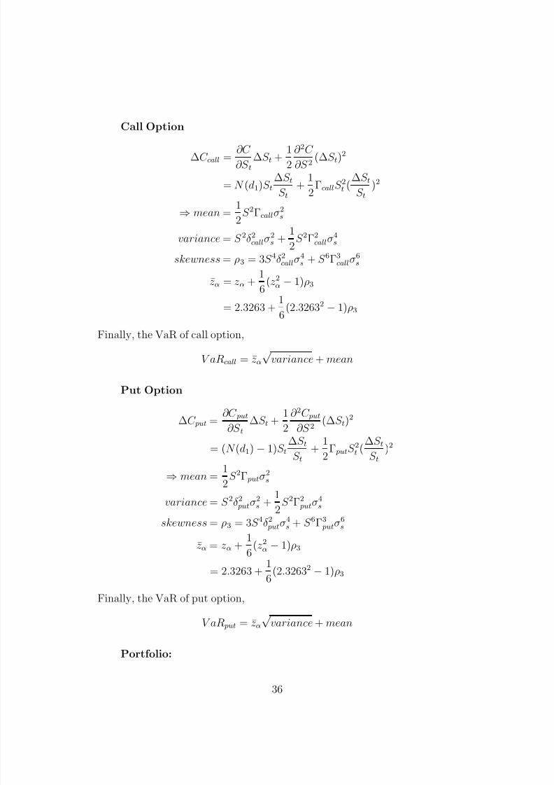
Portfolio:
36

8/10/2019 RIsk Valuation in Equity and Interest Rates Risk Factors
http://slidepdf.com/reader/full/risk-valuation-in-equity-and-interest-rates-risk-factors 38/85

8/10/2019 RIsk Valuation in Equity and Interest Rates Risk Factors
http://slidepdf.com/reader/full/risk-valuation-in-equity-and-interest-rates-risk-factors 39/85
We review the first and second derivatives of the ATM call option with respect
to both the risk factors, stock price and interest rate.
δ r = ∂C atmcall
∂rt
= N (a1)S tB
v − kB exp−A−Brt N (a2)
1
v + kB2 exp−A−Brt N (a2)
δ s = ∂C atmcall
∂S t= N (a1)
Γs = ∂ 2C atmcall
∂S 2t=
N (a1)
vS t
Γr = ∂ 2C atmcall
∂r2t
= −B2kS tN (a1)
v2 +
B2kP a2N (a2)
v2 − 2kB2P
v N (a2) − kB2P N (a2)
Γs,r = ∂C atmcall
∂S t∂rt
= N (a1)Bv
Γr,s = ∂C atmcall
∂rt∂S t=
a1BN (a1)
v2 +
kPBa2N (a2)
S tv2 +
kPBN (a2)
S tv
where we have denoted A(t, T ) = A, B(t, T ) = B, v(t, T ) = v, kr = kand P = P (t, T ) = exp−A−Brt be the price of bond. We note that N (x) =1√ 2π
exp −12
x2. Next we have the covariance Σ, aggregated delta δ and gamma
terms Γ, Σ =
σ2
s 00 σ2
r
δ =
S tδ srtδ r
Γ =
ΓsS 2t ΓS,rS trt
ΓS,rS trt Γrr2t
, where we
have assumed that the risk factors are independent. The variables are nowready to be applied to the first four moments of the Cornish-Fisher expan-sion, as well as the skewness ρ3 and kurtosis ρ4, to obtain the approximatedα quantile z α from equation 2.52. Thus, the VaR of the call option withstochastic interest rates is,
V aRatmcall = z α√
µ2 + µ1
Zero Coupon Bond
∆P = ∂P
∂rt
∆rt + 1
2
∂ 2P
∂r2
t
∆r2t
since the partial derivatives are δ bond = ∂P ∂rt
= −D∗P , Γbond = ∂ 2P ∂r2t
= CP ,
where D∗ = T 1+r
and C = T (T +1)(1+r)2
represents the modified duration andconvexity of the zero coupon bond. We get
⇒ ∆P = −D ∗ P ∆rt + 1
2CP ∆r2t
= −( T
1 + r)P ∆rt +
1
2[T (T + 1)
(1 + r)2 ]P ∆r2t
38

8/10/2019 RIsk Valuation in Equity and Interest Rates Risk Factors
http://slidepdf.com/reader/full/risk-valuation-in-equity-and-interest-rates-risk-factors 40/85
⇒mean =
1
2r2Γbondσ2
r
variance = r2δ 2bondσ2s +
1
2r2Γ2
bondσ4r
skewness = ρ3 = 3S 4δ 2bondσ4r + S 6Γ3
bondσ6r
z α = z α + 1
6(z 2α − 1)ρ3
Finally, the VaR of zero coupon bond,
V aRbond = z α√
variance + mean
Therefore, the VaR of portfolio V aR p
V aR p =
V aR2atmcall + V aR2
bond
where we have made the same assumption that the correlation between riskfactors are zero.
MONTE CARLO
1. Euler Scheme
For the Monte Carlo case, we start off by simulating stock prices and shortrates for each time interval. Generated sample paths are of matrix formwhere the rows represent each scenario the stock price or interest could takeat each time. The following matlab codes were taken from [58]:
• blackScholesCallPrice
• generateBSPaths
• monteCarloVar
• monteCarloCVar
Euler Scheme for Stock Prices
An implemented matlab code was used such that it simulates the BlackScholes price process. For portfolio 1 and 2, we are required to generate stockprice paths, which allows us to formulate distributions of call and put option
39
8/10/2019 RIsk Valuation in Equity and Interest Rates Risk Factors
http://slidepdf.com/reader/full/risk-valuation-in-equity-and-interest-rates-risk-factors 41/85
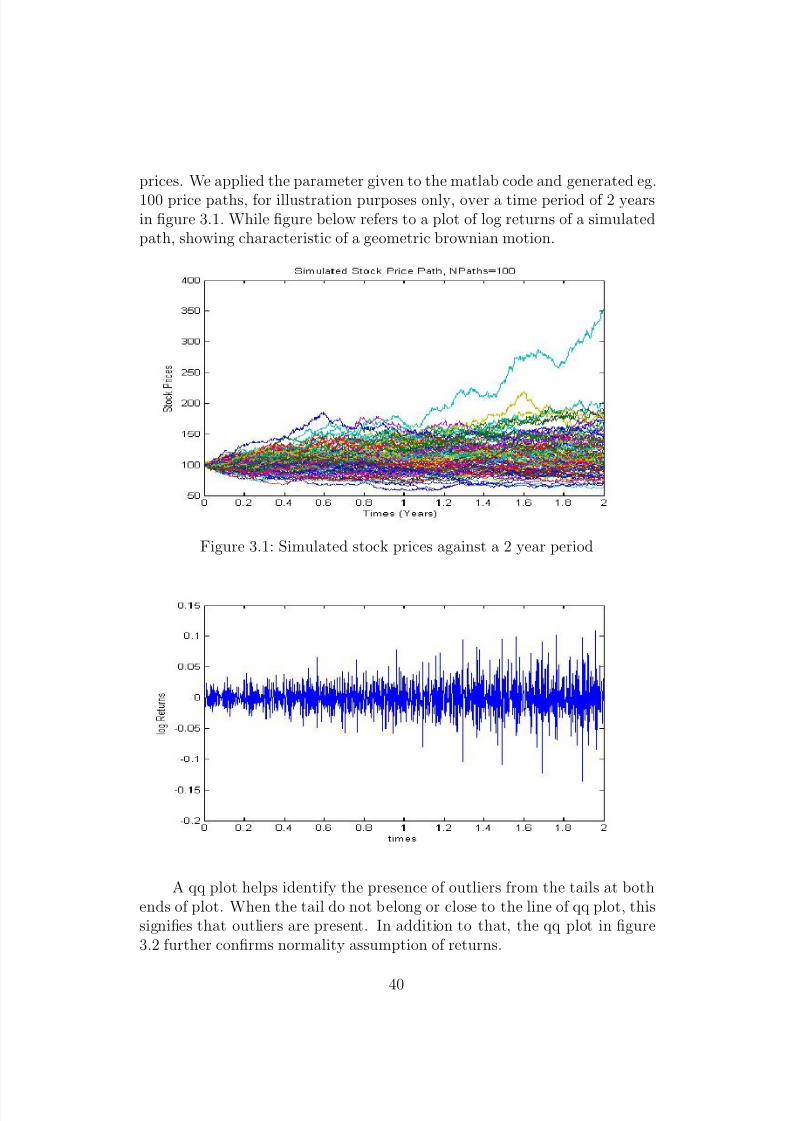
prices. We applied the parameter given to the matlab code and generated eg.
100 price paths, for illustration purposes only, over a time period of 2 yearsin figure 3.1. While figure below refers to a plot of log returns of a simulatedpath, showing characteristic of a geometric brownian motion.
Figure 3.1: Simulated stock prices against a 2 year period
A qq plot helps identify the presence of outliers from the tails at bothends of plot. When the tail do not belong or close to the line of qq plot, thissignifies that outliers are present. In addition to that, the qq plot in figure3.2 further confirms normality assumption of returns.
40

8/10/2019 RIsk Valuation in Equity and Interest Rates Risk Factors
http://slidepdf.com/reader/full/risk-valuation-in-equity-and-interest-rates-risk-factors 42/85
Figure 3.2: QQ Plot of Simulated Stock Price
Euler Scheme for Interest Rates
As required for portfolio 2, interest rates are stochastic such that they evolverandomly over time. The matlab code required for this is simulateVasicek.
We have simulated interest rates under the Vasicek model for each time stepusing the parameters set up for us. Again, for figure 3.3 we have sampled atotal of eg, 100 different scenarios that a short rate can take at each point intime.
41

8/10/2019 RIsk Valuation in Equity and Interest Rates Risk Factors
http://slidepdf.com/reader/full/risk-valuation-in-equity-and-interest-rates-risk-factors 43/85
Figure 3.3: Simulated Interest Rates over a 2 year period
2. Generate Derivative Prices
Our next step of full Monte Carlo simulation is to utilize the simulated pathsto calculate option as well as bond prices for each scenario. These prices were
calculated in the risk neutral measure Q, where the Black-Scholes pricingmodel for each option was properly derived in section 2.3.
Portfolio 1
1. First we generate simulated paths with the matlab code, generateB-SPaths, over a 1 year horizon, since we want a 1-year VaR value. Werun the simulation with a total of 1000 paths.
2. We use the blackScholesCallPrice and blackScholesPutPrice code
to evaluate option prices with a constant rate, r0 = 0.01. We obtainthe distribution of prices by subtracting the put prices from the callprices.
(a) A step consistent with the VaR definition would be to obtain the(100 − α), α = 99%, percentile of the distribution to give us theexpected price.
(b) In the ES case, we measure the mean of the (100 − α) percentileof the distribution with expectedShortfall.
42
8/10/2019 RIsk Valuation in Equity and Interest Rates Risk Factors
http://slidepdf.com/reader/full/risk-valuation-in-equity-and-interest-rates-risk-factors 44/85
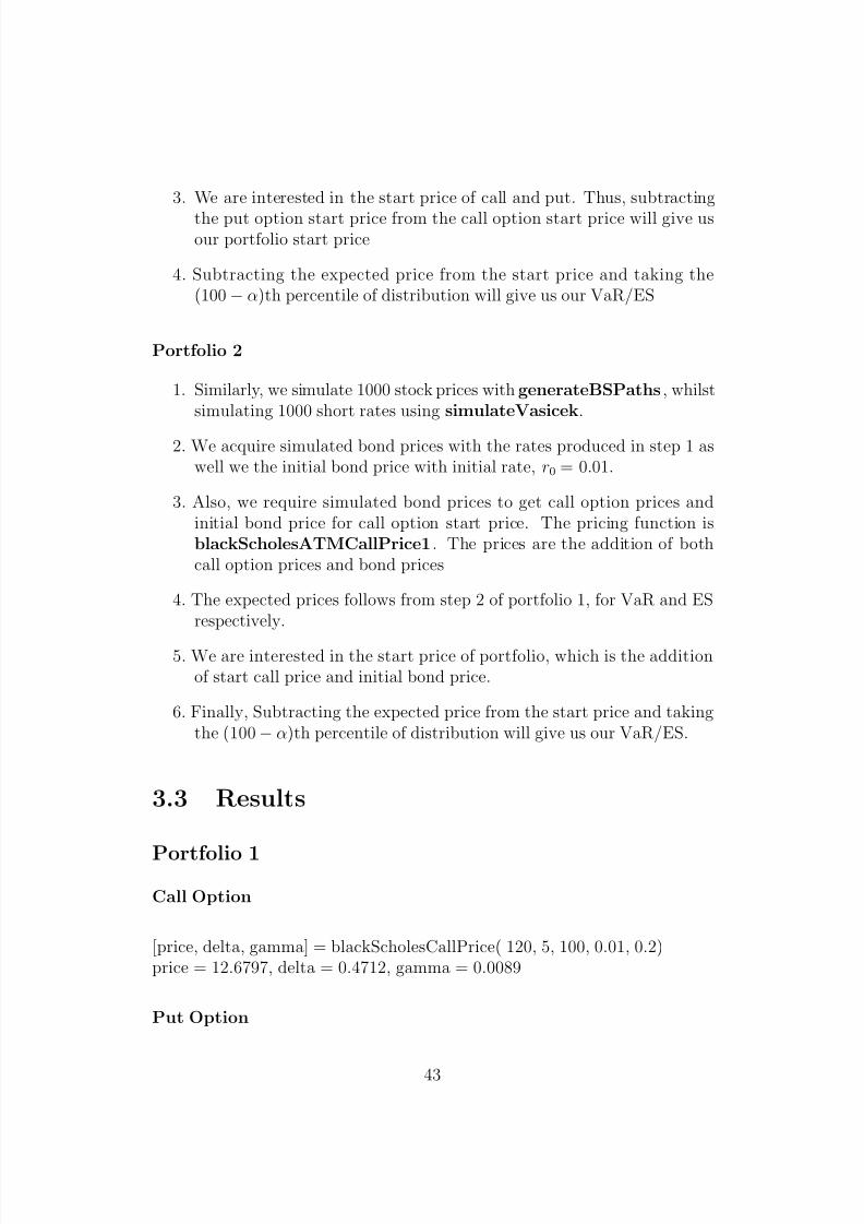
3. We are interested in the start price of call and put. Thus, subtracting
the put option start price from the call option start price will give usour portfolio start price
4. Subtracting the expected price from the start price and taking the(100 − α)th percentile of distribution will give us our VaR/ES
Portfolio 2
1. Similarly, we simulate 1000 stock prices with generateBSPaths, whilstsimulating 1000 short rates using simulateVasicek.
2. We acquire simulated bond prices with the rates produced in step 1 aswell we the initial bond price with initial rate, r0 = 0.01.
3. Also, we require simulated bond prices to get call option prices andinitial bond price for call option start price. The pricing function isblackScholesATMCallPrice1. The prices are the addition of bothcall option prices and bond prices
4. The expected prices follows from step 2 of portfolio 1, for VaR and ESrespectively.
5. We are interested in the start price of portfolio, which is the additionof start call price and initial bond price.
6. Finally, Subtracting the expected price from the start price and takingthe (100 − α)th percentile of distribution will give us our VaR/ES.
3.3 Results
Portfolio 1
Call Option
[price, delta, gamma] = blackScholesCallPrice( 120, 5, 100, 0.01, 0.2)price = 12.6797, delta = 0.4712, gamma = 0.0089
Put Option
43

8/10/2019 RIsk Valuation in Equity and Interest Rates Risk Factors
http://slidepdf.com/reader/full/risk-valuation-in-equity-and-interest-rates-risk-factors 45/85
[price, delta, gamma] = blackScholesCallPrice( 80, 5, 100, 0.01, 0.2)
price = 6.3791, delta =-0.2020, gamma = 0.0063
Portfolio 2
Call Option
[ price, deltaS, gammaS, deltaR, gammaR, gammaSR, gammaRS] = blackSc-holesATMCallPrice(0.1, 100, 5, 100, 0.004, 0.2, 0.01, 0.05)price = 21.6785, deltaS = 0.6665, gammaS = 0.0081, deltaR =319.8334,
gammaR = -1.2093e+003, gammaSR = 3.1998, gammaRS = -3.0708
Zero Coupon Bond
[price, delta, a, b, gamma]= bondPrice( 0.05, 0.1, 5, 0.004, 0.01)price = 0.9118, delta = -4.5137, a = 0.0530, b = 3.9347, gamma = 26.8138
The results above show the corresponding matlab functions used toachieve prices of the options and bond. The first and second partial dif-ferentiation of option price with respect to underlying risk factors were also
successfully calculated. As expected, the delta value of the call option fromportfolio 1 is between 0 and 1, while the delta value for put option falls be-tween -1 and 0. The ATM call option was typically harder and more complexto price as it incorporates stochastic features of stock price and interest rates.The presence of stochastic interest rates greatly affects the price of the op-tion. A high delta such as deltaR=319.8334 indicates that the option priceis very responsive to changes in interest rates, where a small change in ratesresult in a large difference in option price. This could result in a vulnerableportfolio with high market risk. The delta of bond appears to be negative,suggests that an increase in interest rate will have an adverse effect on price
change.
44
8/10/2019 RIsk Valuation in Equity and Interest Rates Risk Factors
http://slidepdf.com/reader/full/risk-valuation-in-equity-and-interest-rates-risk-factors 46/85
Methods Total
Delta Normal VaR
Portfolio 1 Call 21.9293 31.3232Put -9.4001
Portfolio 2 Call -15.9356 15.9356Bond -0.0179
Delta Gamma VaR
Portfolio 1 Call 16.7942 29.5986Put 16.7887
Portfolio 2 Call 36.9990 36.999Bond 0.000179
Monte Carlo VaR
Portfolio 1 Call 11.3153 22.2272Put 5.9907
Portfolio 2 Call 12.1212 12.0953Bond -0.0051
Monte Carlo ES
Portfolio 1 Call 11.6567 25.5905Put 6.0842
Portfolio 2 Call 12.1457 12.1532Bond -0.0064
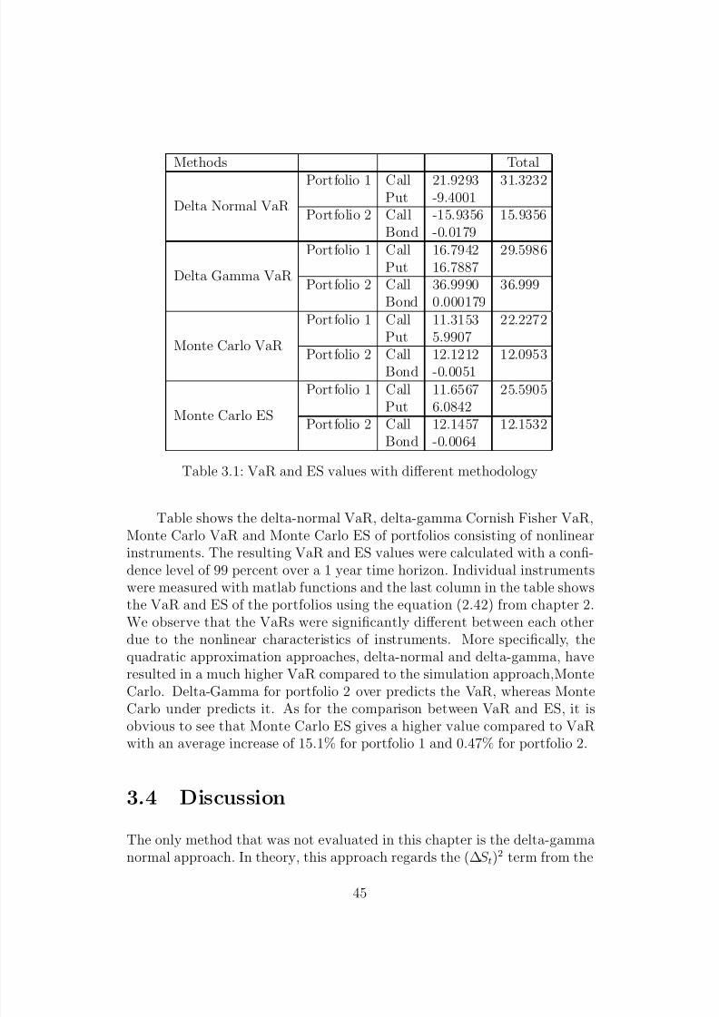
Table 3.1: VaR and ES values with different methodology
Table shows the delta-normal VaR, delta-gamma Cornish Fisher VaR,
Monte Carlo VaR and Monte Carlo ES of portfolios consisting of nonlinearinstruments. The resulting VaR and ES values were calculated with a confi-dence level of 99 percent over a 1 year time horizon. Individual instrumentswere measured with matlab functions and the last column in the table showsthe VaR and ES of the portfolios using the equation (2.42) from chapter 2.We observe that the VaRs were significantly different between each otherdue to the nonlinear characteristics of instruments. More specifically, thequadratic approximation approaches, delta-normal and delta-gamma, haveresulted in a much higher VaR compared to the simulation approach,MonteCarlo. Delta-Gamma for portfolio 2 over predicts the VaR, whereas Monte
Carlo under predicts it. As for the comparison between VaR and ES, it isobvious to see that Monte Carlo ES gives a higher value compared to VaRwith an average increase of 15.1% for portfolio 1 and 0.47% for portfolio 2.
3.4 Discussion
The only method that was not evaluated in this chapter is the delta-gammanormal approach. In theory, this approach regards the (∆S t)
2 term from the
45

8/10/2019 RIsk Valuation in Equity and Interest Rates Risk Factors
http://slidepdf.com/reader/full/risk-valuation-in-equity-and-interest-rates-risk-factors 47/85
second order Taylor’s expansion as another independently distributed normal
variable, say ∆U t. This method treats the model in a way similar to the deltanormal approach as it aims to preserve linear normality. As in [25], Dowdexplains that if ∆S t is normally distributed then (∆S t)
2 must be chi squared.Thus, the assumption will eventually lead to a chi squared ∆C which wouldresult in an unreliable estimation of VaR. For that reason, the delta-gammanormal method was not analyzed in this paper.
In the above calculation, VaR was assessed using the linear and quadraticapproximations. Both options and zero coupon bonds evolves in a nonlinearfashion. To examine precision of approximations, we compute graphs whichrelates option and bond prices to varying stock prices and interest rates. Toillustrate further, we’ve made comparisons between delta and gamma approx-imations with Black-Scholes being regarded as the ”true” value. In figure 3.4and 3.5, we observe that the gamma is lower and much closer to the BlackScholes value compared to delta.
Figure 3.4: Graph of Call value to stock prices using Black-Scholes value,
Delta approximation and Delta Gamma approximation
46

8/10/2019 RIsk Valuation in Equity and Interest Rates Risk Factors
http://slidepdf.com/reader/full/risk-valuation-in-equity-and-interest-rates-risk-factors 48/85
Figure 3.5: Graph of Put value to stock prices using Black-Scholes value,Delta approximation and Delta Gamma approximation
Figure 3.6: Graph of Bond value to interest rates using Vasicek model bondvalue, Delta approximation and Delta Gamma approximation
This suggests that gamma approximations provides better VaR esti-mates for nonlinear derivatives. In the case of zero coupon bond values,initially gamma seems to provide better approximation of bond prices forrates ranging from 0 to 0.4. As short rates increase gamma deviates fur-ther away from Vasicek bond value more compared to delta. Despite that,
47

8/10/2019 RIsk Valuation in Equity and Interest Rates Risk Factors
http://slidepdf.com/reader/full/risk-valuation-in-equity-and-interest-rates-risk-factors 49/85
the difference between delta and gamma to Vasicek value is insignificant.
It is safe to say that delta normal provides sufficiently good estimates forlinear derivatives. Unfortunately, this is not true when considering nonlin-ear derivatives (Options and zero coupon bonds) as it does not account forchanges in volatility. Thus, delta gamma Cornish Fisher approach to VaR ismore favorable.
The deviations between approximation and simulation approach is sig-nificantly high, especially portfolio 2. The reason that may have caused thisis the fact that the ATM call option, which is driven by both stock pricesand short rates, have unique price structure that is difficult for quadratic ap-proximations to capture. This results in an overestimated VaR value. MonteCarlo typically provides good estimation for VaR because it reevaluates thevalue of portfolio for every scenario that may occur with underlying riskfactors. Despite that, large number of simulations is needed to obtain a sub-stantially good estimation of VaR, which causes a lag in calculation. Withthat being said, the number of simulations used in this paper is insufficient.Nevertheless, Monte Carlo is commonly used due to its flexibility and abilityto operate any model of risk factors for determining portfolio’s value in everyscenario.
VaR measure appears to be an exceptional risk management tool for
financial and non financial institutions as it aims to capture market riskand implement useful capital information for banks. In recent years, theshortcomings of VaR became more apparent because of it’s inability to cap-ture credit risk, market liquidity risk or other basis risk. As in [8, p. 9],the committee commented that the VaR capital framework might not bean appropriate from the perspective of banking system. To overcome theseweakness, the committee proposed to the use of ES as an alternative to VaR.ES acts as a better risk measure for several reasons. It follows from [45]
• ES takes into account the tail of the distribution beyond a certain con-fidence level allowing for broader range of unfortunate outcomes. Thisinformation is more convincing for regulators as well as shareholders.This can be observed from our result, where ES takes a larger valuecompared to VaR.
• The coherent and subadditive feature that VaR lacks.
48

8/10/2019 RIsk Valuation in Equity and Interest Rates Risk Factors
http://slidepdf.com/reader/full/risk-valuation-in-equity-and-interest-rates-risk-factors 50/85
Chapter 4
ESTIMATION
Risk measures quickly became the one of the most intriguing area of studywhere researches aim to address the flaws in methods that might have causedfinancial downfall. As such, risk management analysis remains challengingsuch that risk measures are subject to large amounts of risk, eg. model risk.Model risk arises inevitably when a model is fails to perform in such a waythat the value of instruments does not match observed data in the market.Flaws and changes in structure of models can have relatively large impact on
distribution of losses. Apart from risk measures, misvaluation of instrumentsmay incur significant losses from incorrect hedging and investment strategies.
To ensure efficient performance in risk management analysis, it is im-portant to adequately estimate the parameters of the models used. Anothermethod of obtaining the parameters of the model is to calibrate to marketprices. the concept of estimation is different from calibration. Estimationuses statistical method by means of historical values to estimate parameters,in attempt to fit a model to data. Maximum likelihood is an example of estimation, where the density of the model is obtained with a log likelihoodthat we wish to maximize numerically.
On the contrary, the calibration concept does not rely on historical data.Instead, it requires current observed prices in the market. Though estima-tion is comparably easier to implement, risk managers turn to calibrationwhen estimation of models become unfeasible. Calibration is essentially anoptimization problem where sum of difference between model price and mar-ket price is minimized. This means that the error is being minimized tofind the estimated parameters that fit data. As a result, the difference inmarketing-to-model value will be greatly reduced, helping mitigate model
49

8/10/2019 RIsk Valuation in Equity and Interest Rates Risk Factors
http://slidepdf.com/reader/full/risk-valuation-in-equity-and-interest-rates-risk-factors 51/85
risk.
In this chapter, we will be introducing basic concepts of calibration andestimation. We will focus on estimation by maximum likelihood estimatorand run examine accuracy of maximum likelihood estimator as we run teston simulated datas. Further into this chapter, we discuss the problems en-countered when MLE was applied to market data, which was extracted fromBloomberg.
4.1 Estimation
4.1.1 Maximum Likelihood
The conventional method for estimation of model parameters is maximumlikelihood estimator (MLE), designed to find the unknown parameters thatbest describes the variable. A MLE is a function of the sample data, X 1, X 2,...,X n,used to obtain the realized value, estimates or parameters , x1, x2,...,xn. Foranalysis, this technique requires a set of observed data and a mathematicalmodel for the distribution. Before we construct the estimators for Vasicekmodel and geometric Brownian motion, we introduce a formal definition of
maximum likelihood.
Definition 4.1.1. (Maximum Likelihood) As in [46], let the distribution of independent identically distributed (iid) random variables be X = (X 1, X 2, X 3,...,X n),each with pdf f X K (xk; θ)|θ ⊆ Θ, k = 1,..,n dependent on the parameter θ ⊆ Θ. The likelihood function is defined as
L(θ) = f X 1,X 2,...,X n(x1, x2,...,xn; θ),
such that f X 1,X 2,...,X n is the joint probability distribution function of variables.Since they are iid, we can rewrite the equation as
L(θ) = f X 1,X 2,...,X n(x1, x2,...,xn; θ) =n
k=1
f X K (xk; θ). (4.1)
We define θ(X ) to be the maximum likelihood estimator of θ that maximizes the likelihood function, such that it solves,
maxθ∈Θ
L(θ) = maxθ∈Θ
nk=1
f X K (xk; θ).
50

8/10/2019 RIsk Valuation in Equity and Interest Rates Risk Factors
http://slidepdf.com/reader/full/risk-valuation-in-equity-and-interest-rates-risk-factors 52/85
More often, it is easier to maximize the log of the likelihood such that
lnL(θ) = ln[n
k=1
f X K (xk; θ)] =n
k=1
f X K (xk; θ).
If the loglikelihood function is differentiable with respect to θk, then the MLE takes values that solve
∂lnL(θ)
∂θk
= 0. (4.2)
Suppose that X depends on unknown parameters (θ1, θ2,...,θn) ∈ Θ, then the maximum likelihood parameters are ( Θ1, Θ2, ..., Θn)
4.1.2 Maximum Likelihood of Black Scholes Model forStock Price
Next we are interested in estimating the parameters of geometric Brownianmotion with dynamics:
dS t = S t(µdt + σsd W t),
The log returns dynamics,
dlnS t = (µ − σ2
2 )dt + σsd W t,
is normally distributed N ((µ − σ2
2 )(ti − ti−1), σ2
s (ti − ti−1)) with pdf
f y(Y ; µ, σ) = 1
S ti
2πσ2(ti − ti−1)exp −
( lnS tilnS ti−1
− (µ − σ2
2 )(ti − ti−1))2
2σ2(ti − ti−1) .
By using estimators θ = (µ, σs), we obtain our desired parameters θ = (µ, σs).We set the time intervals of equal length be δ = ti − ti−1 , σs = σ andlnS ti = Y ti to ease notation. Thus, the likelihood function is
L(θ) =n
i=1
S ti(2πσδ )−12 exp−
( Y tiY ti−1
− (µ − σ2
2 (ti − ti−1))2
2σ2(ti − ti−1) . (4.3)
Taking the logarithms of the equation above gives us the loglikelihood func-tion,
lnL(θ) =n
i=1
S ti(2πσδ )−12 exp−
( Y tiY ti−1
− (µ − σ2
2 (ti − ti−1))2
2σ2(ti − ti−1) (4.4)
51
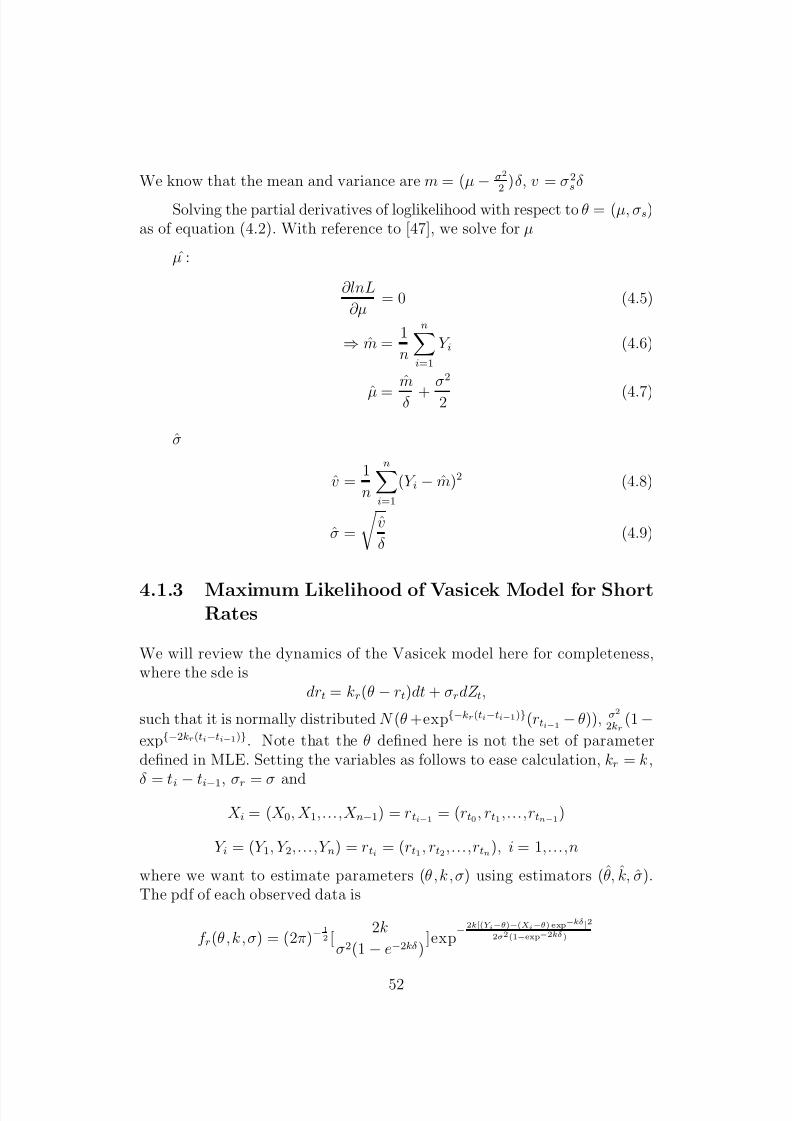
8/10/2019 RIsk Valuation in Equity and Interest Rates Risk Factors
http://slidepdf.com/reader/full/risk-valuation-in-equity-and-interest-rates-risk-factors 53/85
We know that the mean and variance are m = (µ
− σ2
2 )δ , v = σ2
sδ
Solving the partial derivatives of loglikelihood with respect to θ = (µ, σs)as of equation (4.2). With reference to [47], we solve for µ
µ :
∂lnL
∂µ = 0 (4.5)
⇒ m = 1
n
ni=1
Y i (4.6)
µ = m
δ + σ2
2 (4.7)
σ
v = 1
n
ni=1
(Y i − m)2 (4.8)
σ =
v
δ (4.9)
4.1.3 Maximum Likelihood of Vasicek Model for ShortRates
We will review the dynamics of the Vasicek model here for completeness,where the sde is
drt = kr(θ − rt)dt + σrdZ t,
such that it is normally distributed N (θ +exp−kr(ti−ti−1)(rti−1 − θ)), σ2
2kr(1 −
exp−2kr(ti−ti−1). Note that the θ defined here is not the set of parameterdefined in MLE. Setting the variables as follows to ease calculation, kr = k ,
δ = ti − ti−1, σr = σ and
X i = (X 0, X 1,...,X n−1) = rti−1 = (rt0, rt1,...,rtn−1)
Y i = (Y 1, Y 2,...,Y n) = rti = (rt1, rt2,...,rtn), i = 1,...,n
where we want to estimate parameters (θ, k, σ) using estimators (θ, k, σ).The pdf of each observed data is
f r(θ, k, σ) = (2π)−12 [
2k
σ2(1 − e−2kδ)]exp
− 2k[(Y i−θ)−(Xi−θ) exp−kδ ]2
2σ2(1−exp−2kδ)
52

8/10/2019 RIsk Valuation in Equity and Interest Rates Risk Factors
http://slidepdf.com/reader/full/risk-valuation-in-equity-and-interest-rates-risk-factors 54/85
With reference to the literature review in [48], we construct the likelihood
and loglikelihood function, substituting the the quantities.
S y =n
i=1
Y i (4.10)
S x =n
i=1
X i (4.11)
S xx =n
i=1
X 2i (4.12)
S yy =
ni=1
Y 2i (4.13)
S xy =n
i=1
X iY i (4.14)
Also, we let σ2 = σ2(1−exp−2kδ)2k
L =n
i=1
(2π)−12 σ−1 exp
− 1
2 σ2 [(Y i−θ)−(X i−θ)exp−kδ ]2
(4.15)
= (2π)−n2 σ−n exp− 12 σ2n
i=1[(Y i−θ)−(X i−θ)exp−
kδ ]2 (4.16)
lnL = −n
2ln(2π) − nσ − 1
σ2
ni=1
[(Y i − θ) − (X i − θ)exp−kδ ]2 (4.17)
kr :
∂lnL
∂k = −δ exp−kδ
σ2
ni=1
[(θ − X i)(Y i − θ + exp−kδ(θ − X i)2)] = 0 (4.18)
ni=1
(X i − θ)(Y i − θ) = exp−kδ
ni=1
(X i − θ)2 (4.19)
k = −1
δ ln
ni=1(Y i − θ)(X i − θ)n
i=1(X i − θ)2 (4.20)
= −1
δ ln
S xy − θS y − θS x + nθ2
S xx − 2S x − nθ2(4.21)
53

8/10/2019 RIsk Valuation in Equity and Interest Rates Risk Factors
http://slidepdf.com/reader/full/risk-valuation-in-equity-and-interest-rates-risk-factors 55/85
θ:
∂lnL
∂θ =
1
σ2(1 − exp−kδ)
ni=1
[Y i − X i exp−kδ −θ(1 − exp−kδ)] = 0 (4.22)
1
σ2
ni=1
(Y i − X i exp−kδ) − θ
σ2
ni=1
(1 − exp−kδ) = 0 (4.23)
θ = S y − S x exp−kδ
n(1 − exp−kδ)(4.24)
Now we substitute ˆk into
ˆθ,
θ =S y − [S xy−θS y−θS x+nθ2
S xx−2S x−nθ2 ]S x
n[1 − S xy−θS y−θS x+nθ2
S xx−2S x−nθ2 ]
nθ = S y(S xx − 2θS x + nθ2) − (S xy − θS x − θS y + nθ2)S x)
(S xx − 2θS x + nθ2) − (S xy − θS x − θS y + nθ2)
nθ = (S yS xx − S xS xy) + θ(S 2x − S xS y) + θ2n(S y − S x)
S xx − S xy + ˆθ(S y − S x)
Rearranging the terms and we get,
⇒ θ = S yS xx − S xS xy
n(S xx − S xy) − (S 2x − S xS y) (4.25)
σr:
σ2r =
1
n
n
i=1
[(Y i − θ) − exp−kδ(X i − δ )]2
= 1
n
ni=1
[(Y i − θ)2 − 2exp−kδ(X i − θ)(Y i − θ) + exp−2kδ(X i − θ)]2
= 1
n[S yy − 2θS y − θS y + θ2) + exp−2kδ(S xx − 2θS x + θ2)]
= 1
n[S yy − 2exp−kδ S xy + exp−kδ S xx + θ(2exp−kδ S x
+ 2 exp−kδ S y − 2S y − 2exp−2kδ S x) + θ2(1 − 2exp−kδ +exp−2kδ)
54

8/10/2019 RIsk Valuation in Equity and Interest Rates Risk Factors
http://slidepdf.com/reader/full/risk-valuation-in-equity-and-interest-rates-risk-factors 56/85
Finally, we obtain σ
σ = σ2r
2k
1 − exp−2kδ(4.26)
We can choose to obtain θ, then proceed to kr and σr since θ is inde-pendent of other parameters.
4.2 Calibration
4.2.1 Calibration of Black Scholes Option Price
The calibration of option prices is described as an optimization-based cali-bration. In order to calibrate option prices, we require Black Scholes optionprices from section 2.3 of chapter 2. With reference to [50], this approachoperates under Q measure and we want to minimize the error defined as thesum of squared difference between the calculated option price and marketoption price, choosing the parameters that best fit the market.
error =
ni=1
(C model(i) − C market(i))2 (4.27)
where C model(i) represents the ith option price of the model and C market(i)is the ith option price in the market with maturity T and strike price K i.Problems in optimizing may arise when equation (4.27) is not linear or convexas more than one local minima may exist. As suggested by Haugh in [50], wecan address this problem by ”convexifying” this optimization problem. Thiscan be done achieved when a penalty term is introduced into the objectivefunction such that it restricts deviations in estimated values from calibratedvalues of previous days.
4.2.2 Calibration of Vasicek Model for Yield UsingMLE
The Vasicek model has been used by banks to describe the evolution of short rates. When collecting data R(t, τ ), one needs to note that instanta-neous short rates are unobtainable directly from the market. More often, thehistorical yield curves are more interesting such that zero coupon prices of
55
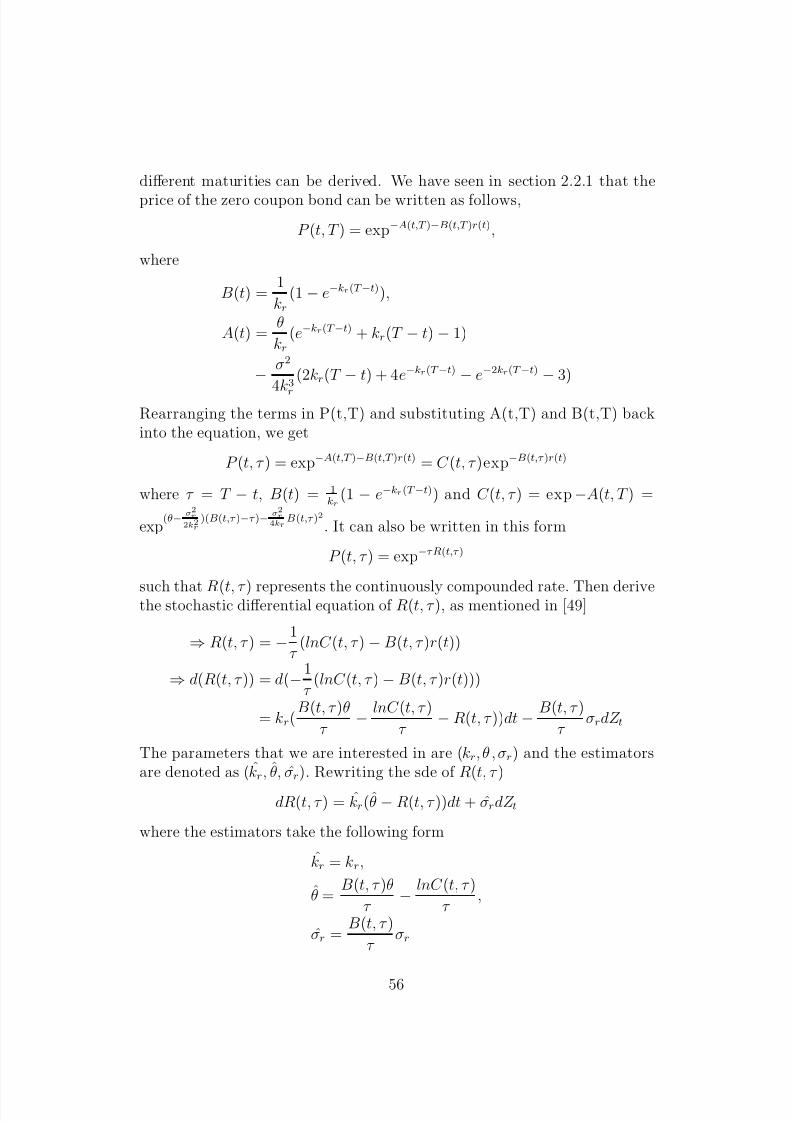
8/10/2019 RIsk Valuation in Equity and Interest Rates Risk Factors
http://slidepdf.com/reader/full/risk-valuation-in-equity-and-interest-rates-risk-factors 57/85
different maturities can be derived. We have seen in section 2.2.1 that the
price of the zero coupon bond can be written as follows,
P (t, T ) = exp−A(t,T )−B(t,T )r(t),
where
B(t) = 1
kr
(1 − e−kr(T −t)),
A(t) = θ
kr
(e−kr(T −t) + kr(T − t) − 1)
−
σ2
4k3
r
(2kr(T
−t) + 4e−kr(T −t)
−e−2kr(T −t)
−3)
Rearranging the terms in P(t,T) and substituting A(t,T) and B(t,T) backinto the equation, we get
P (t, τ ) = exp−A(t,T )−B(t,T )r(t) = C (t, τ )exp−B(t,τ )r(t)
where τ = T − t, B(t) = 1kr
(1 − e−kr(T −t)) and C (t, τ ) = exp −A(t, T ) =
exp(θ− σ2r
2k2r)(B(t,τ )−τ )− σ2r
4kr B(t,τ )2
. It can also be written in this form
P (t, τ ) = exp−τR(t,τ )
such that R(t, τ ) represents the continuously compounded rate. Then derivethe stochastic differential equation of R(t, τ ), as mentioned in [49]
⇒ R(t, τ ) = −1
τ (lnC (t, τ ) − B(t, τ )r(t))
⇒ d(R(t, τ )) = d(−1
τ (lnC (t, τ ) − B(t, τ )r(t)))
= kr(B(t, τ )θ
τ − lnC (t, τ )
τ − R(t, τ ))dt − B(t, τ )
τ σrdZ t
The parameters that we are interested in are (kr, θ , σr) and the estimatorsare denoted as (kr, θ, σr). Rewriting the sde of R(t, τ )
dR(t, τ ) = kr(θ − R(t, τ ))dt + σrdZ t
where the estimators take the following form
kr = kr,
θ = B(t, τ )θ
τ − lnC (t, τ )
τ ,
σr = B(t, τ )
τ σr
56

8/10/2019 RIsk Valuation in Equity and Interest Rates Risk Factors
http://slidepdf.com/reader/full/risk-valuation-in-equity-and-interest-rates-risk-factors 58/85
Using our results by ML estimation, we rearrange the terms to gain ( kr, θ , σr).
kr = kr,
θ = τ θ + lnC (t, τ )
B(t, τ ) ;
σr = σr
4.3 Empirical Analysis
4.3.1 MLE Test for Geometric Brownian motion andVasicek Model for Short Rate
In the previous section, we have discussed about MLE as an estimator forgeometric Brownian motion and Vasicek model. In this section, we will betesting the accuracy of MLE by comparing it with the given parameters forportfolio 1 and 2, specified in chapter 2.
Equity Interest RateMaturity, T 5 years Maturity,T 2 years
Spot Price, S 0 100 Initial Rate, r0 0.01σs 0.2 σr 0.004µ 0.08 kr 0.1
θ 0.05
Table 4.1: The parameters used for the test
The steps on how a proceeded with my test is as follows:
1. First, we simulate one path of stock price over a total of 1000 stepsand ran simulations in matlab, with the function generateBSPaths,using the same euler scheme mentioned in previous chapters.
2. The parameters are then calculated by MLE method, where we haveapplied the simulated stock price to the matlab function, maximum-LEgbm.
3. We repeat steps 1 and 2 by replacing stock price with Vasicek interestrates and obtain parameters with maximumLEVasicek.
57

8/10/2019 RIsk Valuation in Equity and Interest Rates Risk Factors
http://slidepdf.com/reader/full/risk-valuation-in-equity-and-interest-rates-risk-factors 59/85
MLE can be solved numerically by using microsoft excel solver or fmin-
search in matlab. I chose to implement the matlab codes according to theformula derived in section 4.1.2. In step 2, simulated log returns were ob-tained from the simulated stock prices for the calculation.
Next, we compare the results with the original parameters in table 4.2
Equity Interest RateParameter σs µ σr θ kr
True Value 0.2000 0.0800 0.004 0.0500 0.1000MLE value 0.1978 0.1915 0.004 0.0564 0.1216Bias 0.0022 0.1115 0 0.0064 0.0216Bias (%) 0.2200 11.1500 0 0.6400 2.1600
Table 4.2: Comparison of parameters
We can see from the table that MLE gives a reasonably good estimationof the parameters with bias of zero for σr. The parameter kr and µ are mostdifficult ones to estimate as it gave varied bias results with a maximumof 30%. The difficulty in the estimation of the drift parameter, µ, can beresolved when dealing in the risk neutral measure such that the drift rate is
replaced by the risk free rate. The efficiency of estimator increased with thenumber of steps and gave a ridiculously biased results with steps less than100.
4.3.2 Estimation using Raw Data
MLE provides considerably good estimates for geometric Brownian motionand Vasicek model with simulated data. However, it’s performance may varywhen we adopt historical market data into calculations. Thus, this section of the thesis focuses on discussing the performance of MLE and how the chosen
models fare in describing market data.
1. We will be using stock and option prices of Barclays, where the datahave been obtained from Bloomberg with ticker ”BARC LN EQUITY”.I have extracted three years worth of historical stock prices, from8/17/11 to 8/18/14. The call option with the underlying stock, BARC,has a time to expiry of 32 days. Also, i have extracted UK TreasuryBills yield datas from 4/7/14 to 8/18/14, with time to expiry of 48
58

8/10/2019 RIsk Valuation in Equity and Interest Rates Risk Factors
http://slidepdf.com/reader/full/risk-valuation-in-equity-and-interest-rates-risk-factors 60/85
days. Only 5 month yields were taken because it was difficult to get
datas more than 5 months.
2. Figure 4.1 represents the plot of log returns of BARC.L.E. From thefigure below, we can observe 2 major outliers at approximately 0.065years and 0.083 years.
Figure 4.1: Plot of Log Returns
3. Next, the figure 4.2 shows the qq plot of stock prices. This tells usthat our data is Gaussian as most of the datas at the center fall on theline of the qq plot, satisfying the Black Scholes log normality assump-tion on risk factors. Since Vasicek short rate model follows a normaldistribution, as mentioned in section 4.2.2, the yield also follows a nor-mal distribution. From figure 4.3, it can be deduced that the yield of treasury bills satisfies the normality assumption of the Vasicek model.Also, we can observe obvious fat tails at both ends of our plot.
59

8/10/2019 RIsk Valuation in Equity and Interest Rates Risk Factors
http://slidepdf.com/reader/full/risk-valuation-in-equity-and-interest-rates-risk-factors 61/85
Figure 4.2: QQ Plot of Stock Prices
Figure 4.3: QQ Plot of Treasury Bill Yields
Results
Geometric Brownian motion parameters
[mu, sigma] = maximumLEgbm(s, 32/365, 1000)
> mu = −0.7341, > sigma = 2.8204
60
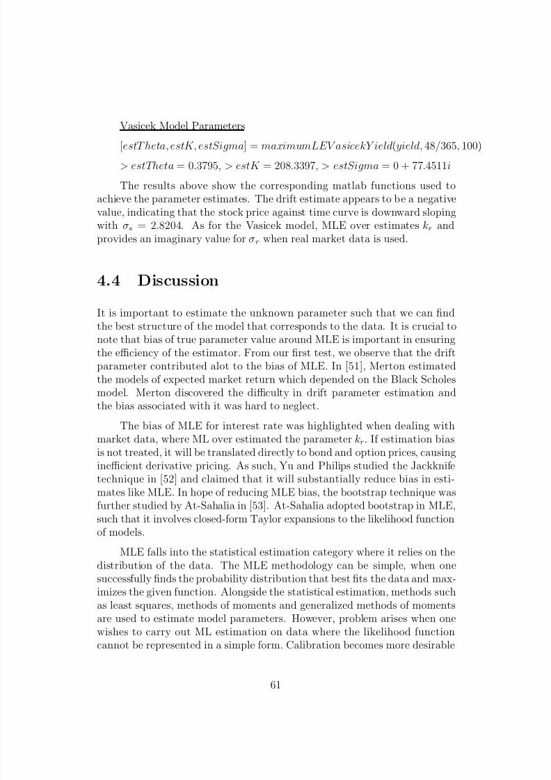
8/10/2019 RIsk Valuation in Equity and Interest Rates Risk Factors
http://slidepdf.com/reader/full/risk-valuation-in-equity-and-interest-rates-risk-factors 62/85
Vasicek Model Parameters
[estT heta, estK, estSigma] = maximumLEV asicekY ield(yield, 48/365, 100)
> estTheta = 0.3795, > estK = 208.3397, > estSigma = 0 + 77.4511i
The results above show the corresponding matlab functions used toachieve the parameter estimates. The drift estimate appears to be a negativevalue, indicating that the stock price against time curve is downward slopingwith σs = 2.8204. As for the Vasicek model, MLE over estimates kr andprovides an imaginary value for σr when real market data is used.
4.4 Discussion
It is important to estimate the unknown parameter such that we can findthe best structure of the model that corresponds to the data. It is crucial tonote that bias of true parameter value around MLE is important in ensuringthe efficiency of the estimator. From our first test, we observe that the driftparameter contributed alot to the bias of MLE. In [51], Merton estimatedthe models of expected market return which depended on the Black Scholesmodel. Merton discovered the difficulty in drift parameter estimation and
the bias associated with it was hard to neglect.The bias of MLE for interest rate was highlighted when dealing with
market data, where ML over estimated the parameter kr. If estimation biasis not treated, it will be translated directly to bond and option prices, causinginefficient derivative pricing. As such, Yu and Philips studied the Jackknifetechnique in [52] and claimed that it will substantially reduce bias in esti-mates like MLE. In hope of reducing MLE bias, the bootstrap technique wasfurther studied by At-Sahalia in [53]. At-Sahalia adopted bootstrap in MLE,such that it involves closed-form Taylor expansions to the likelihood functionof models.
MLE falls into the statistical estimation category where it relies on thedistribution of the data. The MLE methodology can be simple, when onesuccessfully finds the probability distribution that best fits the data and max-imizes the given function. Alongside the statistical estimation, methods suchas least squares, methods of moments and generalized methods of momentsare used to estimate model parameters. However, problem arises when onewishes to carry out ML estimation on data where the likelihood functioncannot be represented in a simple form. Calibration becomes more desirable
61

8/10/2019 RIsk Valuation in Equity and Interest Rates Risk Factors
http://slidepdf.com/reader/full/risk-valuation-in-equity-and-interest-rates-risk-factors 63/85
when risk managers are more interested in calibrating option prices such
that it will be consistent with market option prices. There are similaritiesin methodologies between estimation and calibration, but the differences aresubstantial. Among one of the differences is that calibrated parameters areunder the risk neutral world, Q, and estimated parameters are under realworld, P.
In calibration or estimation, it is important to select a model which isrich in capturing market features. The Black Scholes model is known fornot being able to describe the ”volatility smile” of options in the market.An implied volatility is the volatility value substituted in the Black-Scholesoption pricing equation to retain the market option prices. Black-Scholes’constant volatility assumption implies constant implied volatility across op-tions with different strike prices. However, researches discovered the presenceof volatility smile in implied volatility of market option prices. Thus explainsthe growing number of complex stochastic volatility models such as Heston’smodel in [54]. Heston’s pioneering work, allowed option pricing to take intoaccount correlation between implied volatility and spot asset price. Cali-bration of Heston’s model follows from [55], where Chen Bin explained thelimitations of Black-Scholes pricing model similar to our argument and cal-ibrated Heston’s model. Along the same line of reasoning, it is importantthat the Vasicek model correctly represents the behavior of yield curves. In
[49], Amin compared calibration methods on yield curves, e.g. MLE, LeastSquares method and Kalman Filter. Also, Amin showed that the Vasicekmodel does not provide a good fit for yield curves. The Nelson-Siegel modeland CIR were proven to have shown better yield curve estimates.
62

8/10/2019 RIsk Valuation in Equity and Interest Rates Risk Factors
http://slidepdf.com/reader/full/risk-valuation-in-equity-and-interest-rates-risk-factors 64/85
Chapter 5
CONCLUSION
In this study, we presented some fundamental concepts of the Black-Scholesand Vasicek models. The chosen stochastic models were proposed to describethe behaviors of both equity and interest rate risk factors. Then we appliedour knowledge on VaR and ES calculations by using different methods. Forinstance, delta-normal, delta-gamma Cornish Fisher and Monte Carlo. Wecompared the different approaches and implemented on theoretical portfolios,one of which consists of both equity and interest risks and only equity risk
for the other.The delta-gamma normal method was not analyzed because in [25]
Dowd described it as an inaccurate approach to VaR. In theory, delta-gammaCornish Fisher is a method that provides improved accuracy in risk valua-tion compared to delta-gamma normal. Based on [57], we know that theMonte Carlo method requires more computational effort and underpredictsVaR. Despite that, Monte Carlo VaR and ES values were the most accurateamong the methods. The delta normal methodology yielded incorrect be-havior such that the VaR value was much higher for portfolio 1 and lower forportfolio 2. Overall, matrix methods (e.g. delta normal and delta-gamma
Cornish Fisher) overpredicts VaR. We further examined the Monte Carloapproach to VaR and ES. Our result confirms that ES takes into account of the tail of the distribution, thus yielding a higher value.
In chapter 4, we addressed the issue of model risk in risk valuation bymeans of estimation and calibration. Calibration is much preferred when wewish to calibrate option prices to market option prices. From our analysis, theMLE shows to be a reasonably good parameter estimator of geometric Brow-nian motion and Vasicek model. Unfortunately, this is only the case when
63

8/10/2019 RIsk Valuation in Equity and Interest Rates Risk Factors
http://slidepdf.com/reader/full/risk-valuation-in-equity-and-interest-rates-risk-factors 65/85
dealing with simple portfolios such that it does not have options. The bias
of MLE becomes more apparent when applied to real market data. As dis-cussed in section 4.4, we can reduce the bias by adopting stochastic volatilitymodels that better fits the market data. Thus, significantly reducing modelrisk yields a more efficient risk valuation.
64

8/10/2019 RIsk Valuation in Equity and Interest Rates Risk Factors
http://slidepdf.com/reader/full/risk-valuation-in-equity-and-interest-rates-risk-factors 66/85
Chapter 6
APPENDIX
6.1 Matlab Code for Chapter 3
Simulate Black Scholes stock prices
function[S, times] = generateBSPaths(T, S 0, mu, sigma, nP aths, nSteps)
dt = T/nSteps;
logS 0 = log(S 0);W = randn(nPaths, nSteps);
dlogS = (mu − 0.5 ∗ sigma ∧ 2) ∗ dt + sigma ∗ sqrt(dt) ∗ W ;
logS = logS 0 + cumsum(dlogS, 2);
S = exp(logS );
times = dt : dt : T ;
end
65

8/10/2019 RIsk Valuation in Equity and Interest Rates Risk Factors
http://slidepdf.com/reader/full/risk-valuation-in-equity-and-interest-rates-risk-factors 67/85
Simulate Vasicek short rates
function[r, times] = simulateV asicek(r0,a,b,sigma,T,NPaths,NSteps)
dt = T /N Steps;
times = dt : dt : T ;
r = zeros(NPaths,NSteps);
currR = r0;
fori = 1 : NSteps
epsilon = randn(NPaths, 1);
currR = currR + a
∗(b
−currR)
∗dt + sigma
∗sqrt(dt)
∗epsilon;
r(:, i) = currR;
end
Black Scholes call option price with deterministic interest rate
function[ price, delta, gamma] = blackScholesCallP rice(K , T , S 0,r,sigma)
numerator = log(S 0./K ) + (r + 0.5 ∗ sigma. ∧ 2). ∗ T ;
denominator = sigma. ∗ sqrt(T );
d1 = numerator./denominator;
d2 = d1 − denominator; price = S 0. ∗ normcdf (d1) − exp(−r. ∗ T ). ∗ K. ∗ normcdf (d2);
delta = normcdf (d1);
gamma = normpdf (d1)./(S 0. ∗ denominator);
end
Black Scholes put option price
function[ price, delta, gamma] = blackScholesPutPrice(K , T , S 0,r,sigma)
numerator = log(S 0./K ) + (r + 0.5 ∗ sigma. ∧ 2). ∗ T ;denominator = sigma. ∗ sqrt(T );
d1 = numerator./denominator;
d2 = d1 − denominator;
price = K. ∗ exp(−r. ∗ T ). ∗ normcdf (−d2) − S 0. ∗ normcdf (−d1);
delta = normcdf (d1) − 1;
gamma = normpdf (d1)./(S 0. ∗ denominator);
end
66

8/10/2019 RIsk Valuation in Equity and Interest Rates Risk Factors
http://slidepdf.com/reader/full/risk-valuation-in-equity-and-interest-rates-risk-factors 68/85
Black Scholes call option price with stochastic interest rate
function[ price, deltaS, gammaS, deltaR, gammaR, gammaSR, gammaRS ] =
blackScholesATMCallPrice(k,Strike,T,S 0, sigmaR, sigmaS, r, theta)
[P, ∼, ∼, B] = bondPrice(theta,k,T,sigmaR,r);
v2 = (sigmaR. ∧ 2)./(2. ∗ (k)). ∗ ((2. ∗ k. ∗ T ) + (4. ∗ exp(−k. ∗ T ))−exp(−2. ∗ k. ∗ T ) − (3))+
((sigmaS. ∧ 2). ∗ T );
numerator = log(S 0./(Strike. ∗ P )) + 0.5. ∗ (v2);
v = sqrt(v2);
numerator1 = log(S 0./(Strike. ∗ P )) − 0.5. ∗ (v2);
a1 = numerator./v;
a2 = numerator1./v;
price = S 0. ∗ normcdf (a1) − Strike. ∗ P. ∗ normcdf (a2);
deltaS = normcdf (a1);
gammaS = (normpdf (a1))./(S 0. ∗ v);
deltaR = (normpdf (a1). ∗ B. ∗ S 0)./v − k. ∗ B. ∗ P. ∗ normpdf (a2). ∗ (v. ∧ (−1))+
(k. ∗ P. ∗ B. ∗ normcdf (a2));
gammaR = −((B. ∧ 2). ∗ a1. ∗ S 0. ∗ normpdf (a1))./(v2)+ ((B. ∧ 2). ∗ k. ∗ P. ∗ a2. ∗ normcdf (a2))./v2 ...
+ (2. ∗ k. ∗ P. ∗ (B. ∧ 2). ∗ (normpdf (a2)))./v − k. ∗ (B. ∧ 2). ∗ P. ∗ normcdf (a2);
gammaSR = (normpdf (a1). ∗ B)./(v);
gammaRS = −(B. ∗ a1. ∗ normpdf (a1))./(v2)+
(k. ∗ P. ∗ B. ∗ a2. ∗ normpdf (a2))./(S 0. ∗ v2)+
(k. ∗ P. ∗ B. ∗ normpdf (a2))./(S 0. ∗ v2);
end
67

8/10/2019 RIsk Valuation in Equity and Interest Rates Risk Factors
http://slidepdf.com/reader/full/risk-valuation-in-equity-and-interest-rates-risk-factors 69/85
Vasicek bond price
function[ price, delta, a, b, gamma] = bondPrice(theta,k,T,sigma,r)
modD = T ./(1 + r);
value1 = exp(−k. ∗ T ) + k. ∗ T − 1;
value2 = (2. ∗ k. ∗ T ) + (4. ∗ exp(−k. ∗ T )) − exp(−2. ∗ k. ∗ T ) − 3;
a = (theta./k). ∗ (value1) − ((sigma. ∧ 2)./(4. ∗ (k. ∧ 3))). ∗ (value2);
b = (1./k). ∗ (1 − exp(−k. ∗ T ));
price = exp(−a − (b ∗ r));
delta =
−modD.
∗ price;
gamma = ((T. ∗ (T + 1))./(1 + r). ∧ 2). ∗ price;
end
6.1.1 Delta Normal
Portfolio 1
Delta normal call option with deterministic interest rate
function[deltaNormal] = deltaNormalCall(K , T, S 0, r, sigma, alpha)[∼, delta, ∼] = blackScholesCallPrice(K , T , S 0,r,sigma);
z = norminv(alpha);
deltaNormal = z. ∗ delta. ∗ S 0. ∗ sigma;
end
Delta normal put option
function[deltaNormal] = deltaNormalPut(K , T , S 0, r, sigma, alpha)
[∼, delta, ∼] = blackScholesPutPrice(K , T, S 0,r,sigma);z = norminv(alpha);
deltaNormal = z. ∗ delta. ∗ S 0. ∗ sigma;
end
68

8/10/2019 RIsk Valuation in Equity and Interest Rates Risk Factors
http://slidepdf.com/reader/full/risk-valuation-in-equity-and-interest-rates-risk-factors 70/85
Delta normal of Portfolio 1
function[deltaNormal] = deltaNormalPort1V ar(KCall,KPut,T,t,S 0, r, sigma, alpha)
[∼, deltaCall, ∼] = blackScholesCallP rice(KCall,T,S 0,r,sigma);
[∼, deltaP ut, ∼] = blackScholesPutPrice(KPut,T,S 0,r,sigma);
deltaPort = deltaCall − deltaPut;
z = norminv(alpha);
deltaNormal = z. ∗ deltaPort. ∗ S 0. ∗ sigma;
end
Portfolio 2
Delta normal call option with stochastic interest rate
function[deltaNormal] = deltaNormalAT M Call(k,Strike,T,S 0,...
sigmaR, r, theta, alpha, sigmaS )
[∼, deltaS,∼, deltaR,∼, ∼, ∼] = blackScholesAT MCallP rice(...
k,Strike,T,S 0, sigmaR, sigmaS, r, theta);
z = norminv(alpha);
std = sqrt(((deltaS. ∗ S 0). ∧ 2). ∗ (sigmaS. ∧ 2)+
((deltaR. ∗ r). ∧ 2). ∗ (sigmaR. ∧ 2));
deltaNormal = z. ∗ std;
end
Delta normal bond
function[deltaNormal] = deltaNormalBond(theta, k, T, sigma, r, alpha)
[∼, delta, ∼, ∼, ∼] = bondPrice(theta,k,T,sigma,r );
z = norminv(alpha);deltaNormal = −z. ∗ delta. ∗ sigma;
end
69

8/10/2019 RIsk Valuation in Equity and Interest Rates Risk Factors
http://slidepdf.com/reader/full/risk-valuation-in-equity-and-interest-rates-risk-factors 71/85
6.1.2 Delta-Gamma
Delta gamma call option
function[var] = deltaGammaV ar(S,K,T,r,sigma,alpha)
[∼, delta, gamma] = blackScholesCallP rice(K,T,S,r,sigma);
zalpha = norminv(alpha);
mean = (0.5). ∗ (S. ∧ 2). ∗ gamma. ∗ (sigma. ∧ 2);
variance = (S. ∧ 2). ∗ (delta. ∧ 2). ∗ (sigma. ∧ 2)...
+ 0.5. ∗ (S. ∧ 4). ∗ (gamma. ∧ 2). ∗ (sigma. ∧ 4);
coeff = 3. ∗ (S. ∧ 4). ∗ (delta. ∧ 2). ∗ gamma. ∗ (sigma. ∧ 4)+ (S. ∧ 6). ∗ (gamma. ∧ 3). ∗ (sigma. ∧ 6);
rho3 = coeff./(sqrt(variance). ∧ 3);
zalpha1 = zalpha − (1./6). ∗ ((zalpha. ∧ 2) − 1). ∗ rho3;
var = (zalpha1. ∗ (sqrt(variance))) + mean;
end
Delta gamma put option
function[var] = deltaGammaPut(K,T,S,r,sigma,alpha)z = norminv(alpha);
[∼, delta, gamma] = blackScholesPutPrice(K,T,S,r,sigma);
mean = (0.5). ∗ (S. ∧ 2). ∗ gamma. ∗ (sigma. ∧ 2);
variance = (S. ∧ 2). ∗ (delta. ∧ 2). ∗ (sigma. ∧ 2)...
+ 0.5. ∗ (S. ∧ 4). ∗ (gamma. ∧ 2). ∗ (sigma. ∧ 4);
coeff = 3. ∗ (S. ∧ 4). ∗ (delta. ∧ 2). ∗ gamma. ∗ (sigma. ∧ 4)
+ (S. ∧ 6). ∗ (gamma. ∧ 3). ∗ (sigma. ∧ 6);
rho3 = coeff./(sqrt(variance).
∧3);
zalpha = z + (1./6). ∗ ((z. ∧ 2) − 1). ∗ rho3;
var = (zalpha. ∗ (sqrt(variance))) + mean;
end
70

8/10/2019 RIsk Valuation in Equity and Interest Rates Risk Factors
http://slidepdf.com/reader/full/risk-valuation-in-equity-and-interest-rates-risk-factors 72/85
Delta gamma of Portfolio 1
function[deltaGamma] = deltaGammaPort1V ar(KCall,KPut,...
T,S,r,sigma,alpha)
[∼, deltaCall, gammaCall] = blackScholesCallP rice(KCall,T,S,r,sigma);
[∼, deltaP ut, gammaP ut] = blackScholesPutPrice(KPut,T,S,r,sigma);
delta = deltaCall − deltaPut;
gamma = gammaCall − gammaPut;
zalpha = norminv(alpha);
mean = (0.5).
∗(S.
∧2).
∗gamma.
∗(sigma.
∧2);
variance = (S. ∧ 2). ∗ (delta. ∧ 2). ∗ (sigma. ∧ 2)...
+ 0.5. ∗ (S. ∧ 4). ∗ (gamma. ∧ 2). ∗ (sigma. ∧ 4);
coeff = 3. ∗ (S. ∧ 4). ∗ (delta. ∧ 2). ∗ gamma. ∗ (sigma. ∧ 4)
+ (S. ∧ 6). ∗ (gamma. ∧ 3). ∗ (sigma. ∧ 6);
rho3 = coeff./(sqrt(variance). ∧ 3);
zalpha1 = zalpha − (1./6). ∗ ((zalpha. ∧ 2) − 1). ∗ rho3;
deltaGamma = (zalpha1. ∗ (sqrt(variance))) + mean;
end
71

8/10/2019 RIsk Valuation in Equity and Interest Rates Risk Factors
http://slidepdf.com/reader/full/risk-valuation-in-equity-and-interest-rates-risk-factors 73/85
Delta gamma of call option with stochastic interest rate
function[deltaGamma] = deltaGammaATM Callvar(alpha,k,Strike,T,
S 0, sigmaR, sigmaS, r, theta)
rho = 0;
[∼, deltaS, gammaS, deltaR, gammaR, gammaSR, gammaRS ] =
blackScholesATMCallPrice(k,Strike,T,S 0, sigmaR, sigmaS, r, theta);
cov = [sigmaS. ∧ 2,rho; rho, sigmaR. ∧ 2];
delta = [S 0. ∗ deltaS ; r. ∗ deltaR];
gamma = [gammaS.
∗(S 0).
∧2, gammaSR.
∗S 0.
∗r;
gammaRS. ∗ S 0. ∗ r, gammaR. ∗ (r. ∧ 2)];
mean = (0.5). ∗ trace(gamma ∗ cov);
variance = (delta) ∗ cov ∗ delta + (0.5). ∗ (trace(gamma ∗ cov)). ∧ 2;
mom3 = 3. ∗ (delta) ∗ cov ∗ (gamma ∗ cov) ∗ delta + (trace(gamma ∗ cov)). ∧ 3;
mom4 = 12. ∗ (delta) ∗ cov ∗ ((gamma ∗ cov). ∧ 2) ∗ delta
+ 3. ∗ (trace(gamma ∗ cov)). ∧ 4...
+ 3. ∗ ((variance). ∧ 2);
rho3 = mom3./((sqrt(variance)). ∧ 3);
rho4 = mom4./((variance). ∧ 2) − 3;zbar = norminv(alpha) + (1./6). ∗ (norminv(alpha). ∧ 2 − 1). ∗ rho3...
+ (1./24). ∗ (norminv(alpha). ∧ 3 − 5. ∗ norminv(alpha)). ∗ rho4...
− (1./36). ∗ (2. ∗ norminv(alpha). ∧ 3 − 5. ∗ norminv(alpha)). ∗ (rho3. ∧ 2);
deltaGamma = zbar. ∗ sqrt(variance) + mean;
end
72

8/10/2019 RIsk Valuation in Equity and Interest Rates Risk Factors
http://slidepdf.com/reader/full/risk-valuation-in-equity-and-interest-rates-risk-factors 74/85
Delta gamma of bond
function[var] = deltaGammaBond(theta, k, T, sigma, r, alpha)
[∼, delta, ∼, ∼, gamma] = bondPrice(theta,k,T,sigma,r );
zalpha = norminv(alpha);
mean = (0.5). ∗ (r. ∧ 2). ∗ gamma. ∗ (sigma. ∧ 2);
variance = (r. ∧ 2). ∗ (delta. ∧ 2). ∗ (sigma. ∧ 2)...
+ 0.5. ∗ (r. ∧ 4). ∗ (gamma. ∧ 2). ∗ (sigma. ∧ 4);
coeff = 3. ∗ (r. ∧ 4). ∗ (delta. ∧ 2). ∗ gamma. ∗ (sigma. ∧ 4)
+ (r.
∧6).
∗(gamma.
∧3).
∗(sigma.
∧6);
rho3 = coeff./(sqrt(variance). ∧ 3);
zalpha1 = zalpha − (1./6). ∗ ((zalpha. ∧ 2) − 1). ∗ rho3;
var = (zalpha1. ∗ (sqrt(variance))) + mean;
end
73

8/10/2019 RIsk Valuation in Equity and Interest Rates Risk Factors
http://slidepdf.com/reader/full/risk-valuation-in-equity-and-interest-rates-risk-factors 75/85
6.1.3 Monte Carlo VaR
Portfolio 1
Portfolio 1 VaR
function[var] = monteCarloP ort1V ar( percent, days,
strikeCall, strikeP ut, maturity, ...
spot, drif t, volatility, riskF reeRate, nP aths)
t = days/365;
stockPrices = generateBSP aths(t, spot, drif t, volatility, nPaths, 1);callPrices = blackScholesCallPrice(strikeCall, maturity − t, stockP rices, ...
riskF reeRate, volatility);
putP rices = blackScholesPutPrice(strikeP ut, maturity − t, stockP rices, ...
riskF reeRate, volatility);
prices = callPrices − putP rices;
endPrice = prctile( prices, 100 − percent);
startCallPrice = blackScholesCallPrice(strikeCall, maturity, spot, ...
riskF reeRate, volatility);
startPutPrice = blackScholesPutPrice(strikeP ut, maturity, spot, ...
riskF reeRate, volatility);
startPrice = startCallPrice − startPutPrice;
changePrices = startPrice − endPrice;
var = prctile(changePrices,100 − percent);
end
74

8/10/2019 RIsk Valuation in Equity and Interest Rates Risk Factors
http://slidepdf.com/reader/full/risk-valuation-in-equity-and-interest-rates-risk-factors 76/85
Portfolio 2 VaR
function[var] = monteCarloP ort2V ar( percent, days, k, theta, volatilityR...
, strike, maturity, spot, mu, volatilityS, ...riskFreeRate, nPaths)
t = days/365;
stockPrices = generateBSP aths(t, spot, mu, volatilityS, nP aths, 1);
r = simulateV asicek(riskF reeRate, k, theta, volatilityR, t, nPaths, 1);
P = bondPrice(theta, k, maturity − t, volatilityR, r);
callPrices = blackScholesAT MCallP rice1(P, k, strike, maturity − t, ...
stockP rices, volatilityR, volatilityS, r, theta);
prices = callPrices + P ;
endPrice = prctile( prices, 100 − percent);
initialBondPrice = bondPrice(theta, k, maturity, volatilityR, riskF reeRate);
startCallPrice = blackScholesAT MCallP rice1(initialBondPrice, k, strike,
maturity, spot, volatilityR, volatilityS, riskF reeRate, theta);
startPrice = startCallPrice + initialBondPrice;
var = startPrice − endPrice;
end
6.1.4 Monte Carlo ES
Expected shortfall
functioncvar = expectedShortfall( prices, percentage)
cutOff = prctile( prices, 100 − percentage);
tail = prices( prices <= cutOff );
cvar = mean(tail);
end
75

8/10/2019 RIsk Valuation in Equity and Interest Rates Risk Factors
http://slidepdf.com/reader/full/risk-valuation-in-equity-and-interest-rates-risk-factors 77/85
Portfolio 1
function[var] = monteCarloP ort1ES ( percent, days,
strikeCall, strikeP ut, maturity, spot, drif t, volatility, riskF reeRate, nPaths)
t = days/365;
stockPrices = generateBSP aths(t, spot, drif t, volatility, nPaths, 1);
callPrices = blackScholesCallPrice(strikeCall, maturity − t, stockP rices,
riskF reeRate, volatility);
putP rices = blackScholesPutPrice(strikeP ut, maturity − t, stockP rices,
riskF reeRate, volatility);
prices = callPrices − putP rices;
endPrice = expectedShortfall( prices, percent);
startCallPrice = blackScholesCallPrice(strikeCall, maturity, spot, riskF reeRate, volatility);
startPutPrice = blackScholesPutPrice(strikeP ut, maturity, spot, riskF reeRate, volatility);
startPrice = startCallPrice − startPutPrice;
changePrices = startPrice − endPrice;
var = prctile(changePrices,100 − percent);
end
76

8/10/2019 RIsk Valuation in Equity and Interest Rates Risk Factors
http://slidepdf.com/reader/full/risk-valuation-in-equity-and-interest-rates-risk-factors 78/85
Portfolio 2
function[var] = monteCarloP ort2ES ( percent, days, k, theta, volatilityR...
, strike, maturity, spot, mu, volatilityS, riskF reeRate, nPaths)
t = days/365;
stockPrices = generateBSP aths(t, spot, mu, volatilityS, nP aths, 1);
r = simulateV asicek(riskF reeRate, k, theta, volatilityR, t, nPaths, 1);
P = bondPrice(theta, k, maturity − t, volatilityR, r);
callPrices = blackScholesAT MCallP rice1(P, k, strike, maturity − t, ...
stockP rices, volatilityR, volatilityS, r, theta);
prices = callPrices + P ;
endPrice = expectedShortfall( prices, percent);
initialBondPrice = bondPrice(theta, k, maturity, volatilityR, riskF reeRate);
startCallPrice = blackScholesAT MCallP rice1(initialBondPrice, k, strike, maturity, ...
spot, volatilityR, volatilityS, riskF reeRate, theta);
startPrice = startCallPrice + initialBondPrice;
var = startPrice − endPrice;
end
6.2 Matlab Code for Chapter 4
Simulate Vasicek yield
function[y, times] = simulateV asicekY ield(y0,k,theta,sigma,T,NPaths,NSteps)
dt = T /NSteps;
times = dt : dt : T ;
y = zeros(NPaths,NSteps);
currY = y0;
fori = 1 : N Steps
epsilon = randn(NPaths, 1);
currY = currY + k ∗ (theta − currY ) ∗ dt + sigma ∗ sqrt(dt) ∗ epsilon;
y(:, i) = currY ;
end
77

8/10/2019 RIsk Valuation in Equity and Interest Rates Risk Factors
http://slidepdf.com/reader/full/risk-valuation-in-equity-and-interest-rates-risk-factors 79/85
MLE for geometric Brownian motion
function[mu, sigma] = maximumLEgbm(s1,T,nsteps)
s = diff (log(s1));
n = length(s) − 1;
delta = T/nsteps;
mhat = (sum(s(1 : end))./n);
vhat = (sum((s(1 : end) − mhat). ∧ 2)./n);
sigma = sqrt((vhat./delta));
mu = (mhat./delta) + ((sigma ∧ 2) ∗ 0.5);
end
MLE for Vasicek Short Rate
function[theta, k, sigma] = maximumLEV asicek(r, T, nsteps)
delta = T/nsteps;
n = length(r) − 1;
sx = sum(r(1 : end − 1));
sy = sum(r(2 : end));
sxx = sum(r(1 : end
−1).
∧2);
syy = sum(r(2 : end). ∧ 2);
sxy = sum(r(1 : end − 1). ∗ r(2 : end));
num1 = (sy ∗ sxx − sx ∗ sxy);
num2 = (n ∗ (sxx − sxy) − (sx ∧ 2 − sx ∗ sy));
theta = num1/num2;
num3 = (sxy − theta ∗ sx − theta ∗ sy + n ∗ theta ∧ 2);
num4 = (sxx − 2 ∗ theta ∗ sx + n ∗ theta ∧ 2);
k = −(1/delta) ∗ log((num3)/(num4));
expo1 = exp(−k ∗ delta);expo2 = exp(−2 ∗ k ∗ delta);
coeff 1 = syy − (2 ∗ expo1 ∗ sxy) + (expo2 ∗ sxx);
coeff 2 = (2 ∗ expo1 ∗ sx) + (2 ∗ expo1 ∗ sy) − (2 ∗ sy) − (2 ∗ expo2 ∗ sx);
coeff 3 = 1 − (2 ∗ expo1) + expo2;
sigmahat = (1/n) ∗ (coeff 1 + theta ∗ (coeff 2) + (theta ∧ 2) ∗ coeff 3);
sigma = sqrt((sigmahat ∗ 2 ∗ k)/(1 − expo2));
end
78

8/10/2019 RIsk Valuation in Equity and Interest Rates Risk Factors
http://slidepdf.com/reader/full/risk-valuation-in-equity-and-interest-rates-risk-factors 80/85
MLE for Vasicek yield
function[trueT heta, trueK, trueSigma, k, theta, sigma] =
maximumLEV asicekY ield(y,T,nsteps)
delta = T/nsteps;
n = length(y) − 1;
sx = sum(y(1 : end − 1));
sy = sum(y(2 : end));
sxx = sum(y(1 : end − 1). ∧ 2);
syy = sum(y(2 : end).
∧2);
sxy = sum(y(1 : end − 1). ∗ y(2 : end));
num1 = (sy ∗ sxx − sx ∗ sxy);
num2 = (n ∗ (sxx − sxy) − (sx ∧ 2 − sx ∗ sy));
theta = num1/num2;
num3 = (sxy − theta ∗ sx − theta ∗ sy + n ∗ theta ∧ 2);
num4 = (sxx − 2 ∗ theta ∗ sx + n ∗ theta ∧ 2);
k = −(1/delta) ∗ log((num3)/(num4));
expo1 = exp(−k ∗ delta);
expo2 = exp(−2 ∗ k ∗ delta);coeff 1 = syy − (2 ∗ expo1 ∗ sxy) + (expo2 ∗ sxx);
coeff 2 = (2 ∗ expo1 ∗ sx) + (2 ∗ expo1 ∗ sy) − (2 ∗ sy) − (2 ∗ expo2 ∗ sx);
coeff 3 = 1 − (2 ∗ expo1) + expo2;
sigmahat = (1/n) ∗ (coeff 1 + theta ∗ (coeff 2) + (theta ∧ 2) ∗ coeff 3);
sigma = sqrt((sigmahat ∗ 2 ∗ k)/(1 − expo2));
value1 = exp(−k. ∗ T ) + k. ∗ T − 1;
value2 = (2. ∗ k. ∗ T ) + (4. ∗ exp(−k. ∗ T )) − exp(−2. ∗ k. ∗ T ) − 3;
b = (1./k).
∗(1
−exp(
−k.
∗T ));
a = (theta./k). ∗ (value1) − ((sigma. ∧ 2)./(4. ∗ (k. ∧ 3))). ∗ (value2);
c = exp(−a);
trueTheta = ((T. ∗ theta) + log(c))./(b);
trueSigma = (T. ∗ sigma)./b;
trueK = k;
end
79

8/10/2019 RIsk Valuation in Equity and Interest Rates Risk Factors
http://slidepdf.com/reader/full/risk-valuation-in-equity-and-interest-rates-risk-factors 81/85
Bibliography
[1] H. M. Markowitz (1952), Portfolio Selection, The Journal of Fi-
nance , vol. 7, pp. 71-91.
[2] W. F. Sharpe (1964), Capital Asset Prices: A Theory of MarketEquilibrium Under Conditions of Risk, The Journal of Finance , pp. 425-431.
[3] F. Black and M. Scholes (1973), The Pricing Option and Corpo-rate Liabilities, The Journal of Poltical Economy , pp. 637-654.
[4] P. Jorion (1995), Big Bets Gone Bad: Derivatives and Bankruptcy inOrange County, Academic Press .
[5] P. Jorion (1997), Value at Risk: The New Benchmark for ManagingFinancial Risk, McGraw-Hill .
[6] P. Artzner, F. Delbaen, J-M . Ebber and D. Heath (1997),Thinking Coherently, Risk 10 , pp. 68-71
[7] Basel . c on banking supervision (2013), A brief history of theBasel Committee, available at http://www.bis.org .
[8] Basel . c on banking supervision (2013), Fundamental reviewof the trading book: A revised market risk framework, available at
http://www.bis.org .
[9] o. vasicek (1997), An Equilibrium Characterization of The TermStructure, Journal of Economics , pp. 177-188
[10] R . C. Merton (Spring, 1973), Theory of Rational Option Pricing, The Bell Journal of Economics and Management Science , vol. 4, pp. 141-183.
[11] J . P. Morgan (1996), RiskMetrics Technical Document, New York ,4th edition
80

8/10/2019 RIsk Valuation in Equity and Interest Rates Risk Factors
http://slidepdf.com/reader/full/risk-valuation-in-equity-and-interest-rates-risk-factors 82/85
[12] I. V. Girsanov (1960), On transforming a certain class of stochastic
processes by absolutely continuous substitution of measures, Theory Probab. Appl , pp. 285-301.
[13] D. Duffie and Rui. Kan (1996), A Yield-Factor Model of InterestRates, Mathematical Finance , vol. 6, pp. 379-406
[14] M. Dothan (1978), On the Term Structue of Interest Rates, J. Finan-cial Econ , pp. 229-264
[15] T. Ho and S. Lee (1986), Term Structure movements and Pricing In-terest Rate Contingent Claims, J. Finance , pp. 1011-1029
[16] J. B. David (2001), Affine Term-Structure Models: Theory and Imple-mentation, Bank of Canada
[17] D. Brigo and F. Mercusio (2006), Interest Rate Models: TheoryAnd Practice: With Smile, Inflation and Credit, Springer Finance , pp.51-138
[18] D. Heath, R. Jarrow and A. Morton (1992), Bond Pricing andthe Term Structure of Interest Rates: A New Methodology for Contin-gent Claims Valuation, Econometrica , pp. 77-105
[19] R. Gibson, F. S. Lhabitant and D. Talay (2001), Modeling theTerm Structure of Interest Rates: A Review of Literature, Social Science Research Network
[20] J. Hull and A. White (1994), Numerical Procedures for Implement-ing Term Structure Models I: Single-Factor Models, The Journal of Derivatives , pp . 7-16
[21] N. Taleb (2003), Dynamic Hedging - Managing Vanilla and ExoticOptions, Wiley and Sons , pp . 115-146
[22] J. Hull (2008), Options Futures and Other Derivatives, Prentice-Hall ,pp. 291, 342-380
[23] A. McNeil, R. Frey and P. Embrechts (2005), QuantitativeRisk Management: Concepts, Techniques and Tools, Princeton Series in Finance , pp. 34-55, pp. 238-248
[24] K, Dowd (2005), Measuring Market Risk, John Wiley and Sons
81

8/10/2019 RIsk Valuation in Equity and Interest Rates Risk Factors
http://slidepdf.com/reader/full/risk-valuation-in-equity-and-interest-rates-risk-factors 83/85

8/10/2019 RIsk Valuation in Equity and Interest Rates Risk Factors
http://slidepdf.com/reader/full/risk-valuation-in-equity-and-interest-rates-risk-factors 84/85
[39] J. Baran and J. Witzany, A Comparison of EVT and Standard
VaR Estimations, available at http : //ssrn.com/abstract = 1768011 .
[40] M. B. Jones and S. M. Schaefer (1999), Non-Linear Value-at-Risk, European Finance , pp. 161-187
[41] W. Fallon (1996), Calculating Value-at-Risk, working paper,Columbia University
[42] E. A. Cornish and R. A. Fisher (1937), Moments and cumulativein the specification of distributions, Review of the International Statis-tical Institute , pp. 307-320.
[43] B. Tuckman (2002), Fixed Income Securities: Tools for Today’s Mar-ket, John Wiley and Sons , pp. 88-130.
[44] P. Zangari (1996), A VaR methodology for portfolios that includeoptions, RiskMetrics Monitor , PP. 4-12.
[45] Basel . C on banking supervision (2001), Messages From The Aca-demic Literature On Risk Measurement for Trading Book , Working Paper 19 , pp. 20
[46] A. Spanos (2003), Probability Theory and Statistical Inference: Eco-nomic Modeling with Observed Data, Cambridge University Press , pp.660-670
[47] D. Brigo, A. Dalessandro , M. Neugebauer and F. Triki
(2007), A Stochastic Processes Toolkit for Risk Management, availableat http://arxiv.org/pdf/0812.4210.pdf
[48] T. v. d. Berg (2011), Calibrating the Ornstein-Uhlenbeck (Va-sicek) model, available at http://www.sitmo.com/article/calibrating-the-ornstein-uhlenbeck-model/
[49] H. H. N. AMIN (2012), Calibration of Different Interest Rate ModelsFor A Good Fit of Yield Curve, Delft University of Technology
[50] Martin Haugh (2010), Beyond Black Scholes, available at http ://www.columbia.edu/ mh2078/LocalStochasticJumpDiffusion.pdf
[51] R. C. Merton (1980), On Estimating The Expected Return On TheMarket, Journal of Financial Economics , pp. 323-361.
83

8/10/2019 RIsk Valuation in Equity and Interest Rates Risk Factors
http://slidepdf.com/reader/full/risk-valuation-in-equity-and-interest-rates-risk-factors 85/85
[52] Peter C. B. Phillips and J. Yu (2002), Jacknifing of
Bond Options, Review of Financial Studies , available at http ://papers.ssrn.com/abstractid = 373040
[53] YACINE AT-SAHALIA (2008), Closed-form Likelihood Expansionsfor Multivariate diffusions, The Annals of Statistics , pp. 906-937.
[54] Steven. s. heston (1993), A closed-form solution for options withstochastic volatility with applications to bond and currency options, The Review of Financial Studies , vol. 6, pp. 327-343
[55] Chen Bin (2007), Calibration of the Heston Model with Application
in Derivative Pricing and Hedging, University of Delft
[56] Clemens U. Frei (2000), Value at Risk For Linear and Non LinearDerivatives, University of Bielefeld
[57] G. Castellacci and Michael J. Siclari (2003), The practice of DeltaGamma VaR: Implementing the quadratic portfolio model, Euro-pean Journal of Operational Research , pp. 529-545.
[58] Dr. John Armstrong (2014), Numerical and Computational Meth-ods and Computational Methods in Finance, King’s College London ,
Lecture notes 7