Risk-Sharing in the Syndicated LoanMarket: Evidence from Lehman Brothers’

Collapse

Hanh Le ∗†

Abstract

I examine the impact of banks’ liquidity risk on their risk-sharing arrange-

ments in the syndicated loan market. I use Lehman Brothers’ bankruptcy as a

shock to the liquidity risk banks face from revolver draw-downs, and banks’ level

of revolver co-syndication with Lehman as a measure of cross-bank exposure to

this shock. Using within-relationship estimators, I show that more exposed banks

are more likely to reduce the significance of their role in a syndicate. Moreover,

more exposed banks that stay as lead arrangers to the same borrower form more

“diversified” syndicates, choosing syndicate members whose loan portfolios are

less correlated with their portfolios. These adjustments do not occur in term

loans, but only in revolvers, where liquidity risk matters the most. Interestingly,

I find that more exposed banks do not reduce the lending amount, nor do they

charge higher interest rates relative to less exposed banks. Overall, my results

suggest that the ability of banks to limit their liquidity risk exposure via adjust-

ing syndicate structures might alleviate the negative consequences of a shock to

lending supply.

∗University of Illinois at Chicago; email: hanhle@uic.edu†I am grateful to members of my committee: Viral Acharya, Kose John, Anthony Saunders, and

Philipp Schnabl for their guidance and support. For helpful comments, I thank Tobias Berg, DirkBurghardt, Gabriela Coiculescu, Matteo Crosignani, Jason Levine, Anthony Lynch, Rustom Irani,Oliver Randall, Or Shachar, Hyun Song Shin, Stoyan Stoyanov, David Yermack, Shaojun Zhang andseminar participants at NYU-Stern. All errors are mine.

1 Introduction

Syndicated lending facilitates the origination of large loans by pooling together capital

across various lenders, thereby allowing them to share risks. The financial crisis of

2007-2009 presents an experiment to study various aspects of this market. Contraction

of the syndicated lending activity in the wake of the crisis has been extensively inves-

tigated. However, how bank exposure to such a supply-side shock affects risk-sharing

arrangements is an important question that has escaped research attention. This pa-

per aims to provide empirical evidence to this effect. Specifically, I show that banks

which are exposed to negative liquidity shocks during the crisis actively manage their

syndicate structures ways that limits their exposure to future risks. More importantly,

I identify two novel mechanisms through which risk-sharing arrangements can happen:

1. the choice of exit options via the role a lender plays; and 2. the diversification among

syndicate members.

In order to understand how banks share risk when syndicating a loan, it is important

to first understand the risks attached to such a loan. Simply put, a syndicated loan is

one which is jointly provided to a borrower by two or more financial institutions. The

type of the loan determines how much each syndicate member exposes herself to credit

risk and/or liquidity risk. In a term loan contract, banks provide the loan amount

up-front, and the borrower is required to pay interest and principal before the maturity

of the loan. Therefore, a term loan exposes lenders to credit risk, the risk that the

borrower defaults on its repayment obligation. In a revolving line of credit contract

(thereafter referred to as “revolver”), syndicate members are committed to fund on

borrower demand up to the contractual amount of the loan, at any time over the life

of the loan. As such, a revolver not only exposes the lenders to credit risk as in a term

loan, on the amount the borrower has demanded (“drawn down”), but also the liquidity

risk on the amount of undrawn commitments.

1

Each syndicate member chooses her level of risk-sharing in two ways. First, she

may choose the fraction she contributes to the syndicate. The higher the contribution,

the greater the risk to which she is exposed. This aspect has been largely examined

in Sufi (2007), Ball et al. (2008), and Ivashina (2009), among others. Secondly, and

more subtly, she may choose the depth of her involvement in the syndicate by taking on

certain roles. These roles range in the order of importance from “lead arranger” (most

important) to “co-agent” to “participant” (least important).1 While syndicate roles

are typically correlated with the amount of contribution, they differ in whether an exit

option is available. Theoretically, all lenders can sell their shares of a syndicated loan in

the secondary market. Anecdotal evidence suggests that a syndicate’s key lenders rarely

sell loans for fear of reputation damage (see, for example, Ivashina and Sun (2011), Esty

and Megginson (2003)). Because the absence of an option to exit the syndicate increases

the liquidity risk of having funds committed, a more senior syndicate member shares

greater risks compared to a junior one, even when both of them contribute the same

share to the syndicate.

Secondly, I argue that the propensity to share risk by a lead arranger is not only

manifested in her share of the loan, but also in the composition of syndicate members.

Choosing participants whose loan portfolios are distant , i.e. less correlated, with those

of the lead bank will increase the stability of the syndicate. Specifically, a “closer”

syndicate is less likely to fund a commitment when a shock occurs that affects loan

portfolios of both the lead arranger and other participants. Of course, this liquidity

risk-sharing concern should be traded off with the “efficiency hypothesis”, proposed by

Cai et al. (2011), who find that most banks form closer syndicates whose members are

likely to have similar lending expertise, as doing so would reduce the monitoring and

screening costs.

1For a discussion on syndicate roles, please refer to Cai et al. (2011) and Section 2 of this paper.

2

I study how bank exposure to a liquidity shock affects the two aspects of risk-sharing

discussed above. The unexpected collapse of Lehman Brothers in September of 2008,

coupled with the company’s substantial involvement in the syndicated loan market,

provides a useful laboratory to study this question.2 At the time of its bankruptcy

announcement, Lehman had $30 billion in outstanding commitments in the syndicated

loan market. Lehman’s collapse may pose potential liquidity problems for the com-

pany’s revolver cosyndicators (hereafter referred to as “exposed banks”), not because

they now have to stand in for Lehman’s share of the loan, but because they experience

a greater draw-down rate from their borrowers. In fact, these borrowers face liquidity

problems of not being able to borrow from Lehman following its collapse, hence they

may choose to draw down more on other cosyndicators for precautionary purposes.

This places additional stress on exposed banks’ liquidity, potentially leading to a run

on their other revolvers. In fact, Ivashina and Scharfstein (2010) find that draw-downs

occur more for banks that are more exposed to Lehman-cosyndicated revolvers, and

that these draw-downs are largely held in cash.

Given that cosyndicating revolvers with Lehman might subject a bank to the liquid-

ity problems from revolver draw-downs caused by Lehman’s defaulting on its lending

position, I use Lehman’s collapse as a shock to bank’s liquidity and bank-level exposure

to Lehman-cosyndicated revolvers as a cross sectional exposure to this shock. I examine

how this exposure affects the traditional bank lending channel, and subsequently, how

it affects changes in risk-sharing arrangements following Lehman’s collapse. Examining

such supply-side effects is challenging, for the following reasons. First, there could be

a credit demand shock that correlates with bank exposure in the cross section. For

example, suppose more exposed banks are more likely to lend to worse quality firms.

If the systemic crisis set out by Lehman’s collapse forces these firms to go bankrupt in

2Lehman Brothers’ bankruptcy announcement was largely unexpected. On the announcement date,Lehman’s equity lost over 90% of its value.

3

the post-Lehman period, this would have led to a more pronounced drop in lending,

or a mechanical reduction in the depth of roles for more exposed banks. In this case,

any relationship between exposure and the outcome variables are not causal. Second,

exposure to Lehman revolvers is an endogenous choice variable that might depend on

other bank characteristics, which may also drive the observed outcome.

I address the first concern in three ways. Firstly, I control for time varying firm

characteristics that might affect lending and syndicate risk-sharing. Second, I include

borrower industry fixed effects in all regressions, to account for the fact that borrow-

ing firms in different industries may be affected differently by credit demand shocks.

Most importantly, I employ within relationship estimators, effectively including in my

sample only firms that borrow from the same bank both before and after Lehman’s

collapse. This eliminates the sample selection bias caused by unobservables that drive

firms’ decision to borrow. Finally, I include bank-firm fixed effects, which take away

the average of unobservable characteristics driving the bank-firm matching, leaving a

cleaner identification of the exposure effect.

To address the second concern, I examine whether banks with different exposure lev-

els are inherently different from each other. I find that non-exposed banks are smaller,

have more core deposits and less subordinated debt than exposed banks. On the other

hand, banks with positive exposure do not differ very much from each other, except

along the assets dimension. This motivates the use of time-varying bank control vari-

ables in all regressions. Furthermore, compared to exposed banks, non-exposed banks

participate much less frequently in the syndicated loan market. In light of the signifi-

cant difference between exposed and non-exposed banks, I exclude non-exposed banks

from the sample and confirm robustness of the main results.

I find that more exposed banks reduce the maturity of loans originated following

the shock, but do not reduce the lending amount or increase interest rate in the post-

4

Lehman period in any significant way, relative to less exposed banks. At first glance,

this result appears difficult to reconcile with Ivashina and Scharfstein (2010), who find

that banks cosyndicating more revolvers with Lehman decrease their lending during the

financial crisis. However, note that I am only looking at the “intensive lending margin”,

effectively ignoring cases where banks cease to lend to certain borrowers post-event. My

results, coupled with results from Ivashina and Scharfstein (2010) suggest that exposed

banks may ration credit following the shock. Yet for borrowers to whom banks continue

to lend, they do not worsen the terms of loan contracts.

The main contribution of this study is to show that banks may be able to offer

similar lending terms post Lehman by restructuring their risk-sharing arrangements.

Specifically, I find that more exposed banks decrease the significance of their role in

revolvers originated following Lehman’s collapse. A one standard deviation increase in

exposure leads to an 11.5% in probability that the bank switches from an important

role (lead arranger or co-agent) to a participant role. By reducing the importance of

syndicate roles in revolvers, banks subject themselves to less future liquidity risk, as

they are more likely to be able to sell their commitments should liquidity risk arises.

Furthermore, banks are more likely to switch from being a co-agent to a participant,

rather than from a lead arranging role to a less important role. This is expected given

that lead arranging roles are attached with lending relationships that an exposed lender

may not want to forgo.

When examining the cross section of borrowers, I find that exposed banks adjust

the importance of their roles only for the riskiest borrowers, i.e. those without an

investment grade credit rating. As these borrowers have few alternative funding sources,

they are more likely to pose liquidity problems to banks by drawing down on revolvers

for precautionary purposes. The result further reinforces the impact of liquidity risk on

banks’ risk-sharing arrangements, by showing that banks actively manage with which

5

borrowers they choose to increase their exit option.

Given that exposed lead banks do not reduce the depth of their role in revolvers,

do they restructure syndicates in a way that lowers future liquidity risk? To this end, I

find that exposed lead banks are more likely to form more diversified syndicates, where

Cai et al. (2011)’s “distance” measure is adapted as a proxy for lender diversification.

In fact, a one standard deviation increase in the lead bank’s exposure results in a 17%

increase in the measure of lender diversification. By diversifying, an exposed lead bank

subject itself to a smaller liquidity risk, caused by a correlated shock that may affect

liquidity demand or default probability of the borrowers from both the bank and other

syndicate members.

Finally, I examine with which syndicate members an exposed lead bank’s diversifi-

cation concern is the biggest. As co-leads and co-agents (“important lenders”) usually

contribute a larger share to a syndicate, relative to participants, I hypothesize that lead

banks’ diversification incentive is greater when it comes to selecting important lenders.

Indeed, I find that the effect of interest is positive and highly significant when syndicate

diversification is measured as the average distance between lead arrangers and impor-

tant lenders. However, when diversification is measured between the lead arrangers

and participants, the effect of exposure on diversification is still positive but loses its

significance. These results suggest that exposed lead banks reduce their risk exposure

by diversifying with the syndicate members who matter the most for syndicate stability.

My findings have a number of important implications. From a practical standpoint,

they suggest another way in which banks can restructure their assets to manage the

liquidity shock that occurred during the financial crisis, that is, via risk-sharing ar-

rangements in the syndicated loan market. From a theoretical standpoint, my results

pertaining to syndicate diversification suggest the need for theories on syndicated loans

to incorporate lead banks’ ability to select syndicate members. This is in contrast with

6

the traditional banking models of multiple lenders (Diamond (1984), Holmstrom (1979)

and Holmstrom and Tirole (1997)), where the monitoring lender does not have such a

choice. Results presented in this paper imply that managing the composition of lend-

ing syndicates may result in welfare improving outcomes for both the lender and the

borrower.

Related Literature

This study is related to the empirical literature on syndicate structure, whose fo-

cus so far has been primarily on how asymmetric information between borrowers and

lenders, and that among syndicate participants, shapes syndicate ownership arrange-

ments. The literature builds upon the basic theoretical assumption that the need for

lender monitoring arises because of asymmetric information and moral hazard prob-

lems (Leland and Pyle (1977), and Diamond (1984)). Borrowers know their health,

collateral, industriousness better than lenders do (asymmetric information). But they

are not willing to transfer all their information to the lenders, as there are benefits

to exaggerating good attributes and understating bad ones (moral hazard). Diamond

(1984) argues that, when there are many lenders, monitoring efforts are superfluously

costly and may lead to “inefficient free-riding”. As a result, creditors may delegate

monitoring responsibilities to one financial institution. This delegation, nonetheless,

entails moral hazard on the part of the delegated lender. The delegated lender no

longer invests her own money, and therefore she may not have incentives to exert best

effort. In the context of syndicated lending, the lead arranger can be thought of as a

delegated monitor.

A similar moral hazard problem is featured in the framework of Holmstrom (1979)

and Holmstrom and Tirole (1997). Under this framework, there are uninformed lenders,

who rely on information and monitoring provided by the informed lender to make

investments in firms. As the informed lender’s effort is unobservable, she exerts less

7

than first-best optimal effort. This “shirking” behaviour is more costly to the informed

lender the higher her financial interests in the firm. In anticipation of this, uninformed

lenders are only willing to invest in the firm provided the informed lender has taken a

large enough stake. These models lend an explanation for why the lead-arranger, being

the informed lender, should retain a share of the loan; and why she should retain a

larger share when the borrower requires greater monitoring effort.

Dennis and Mullineaux (2000), Jones et al. (2005), and Sufi (2007) provide empir-

ical evidence consistent with such theoretical predictions, showing that the lead share

increases in borrowers’ measures of opacity (e.g. the borrower does not have a public

bond rating, is a private firm, or is non-investment-grade). Ball et al. (2008) proxy

for asymmetric information by the debt-contracting value (DCV) of borrowers, which

captures the ability of firms’ accounting numbers to detect credit quality deterioration

in a timely manner. They find that a higher DCV (i.e. a lower level of information

asymmetry) is associated with a smaller loan share retained by the lead arranger.

In addition to affecting the lead arranger’s share, asymmetric information is also

found to shape other aspects of syndicate structure. Lee and Donald (2004) and Sufi

(2007) find that when there is little information about the borrower, syndicates are

smaller and more concentrated. Lin et al. (2012) argue that firms whose largest ultimate

owner possesses control rights which exceed cash flow rights tend to suffer from moral

hazard problems on the part of such an owner. Consequently, these firms should require

more intense monitoring and due diligence from the lenders, and their lending syndicates

should be formed in a way that facilitates better monitoring. Consistent with this

hypothesis, Lin et al. (2012) find that where the cash flow-control rights divergence is

greater, syndicates are more concentrated and consist of lenders who are close to the

borrower and have lending expertise in the borrower’s industry.

As described above, much work in the area explores how borrower characteristics

8

affect syndicate ownership structure. This study, on the other hand, examines how

lender characteristics shape syndicate structure. In this respect, the study is closest to

Gatev and Strahan (2009), which shows how liquidity risk managements affect syndicate

membership. They find that commercial banks, which hold an advantage relative to

other institution types in providing products exposing lenders to systematic liquidity

risk, dominate the market for revolvers. In addition, commercial banks with a higher

capacity to absorb liquidity risk (as measured by transaction deposits over total assets)

expose themselves to higher liquidity risk via syndicated lines of credit. Findings in

Gatev and Strahan (2009) are consistent with theoretical predictions of Kashyap et al.

(2002), which explain banks’ combination of transaction deposits and credit lines as a

risk management motive. In particular, so long as the demand of depositors and credit

line borrowers are not highly correlated, there exists a benefit in providing liquidity

services to both types of customers. In this study, I focus on novel aspects of syndicate

structure and show that liquidity management does not only manifest in the share of

loan a bank owns, but also in the role in which it is willing to play and the lead bank’s

choice of syndicate members for diversification purposes.

My study is also tangential to a burgeoning strand of literature examining bank

lending during the financial crisis. Ivashina and Scharfstein (2010) is the first attempt

in such a strand to provide evidence of a possible supply-driven lending contraction.

Using Dealscan, a comprehensive database of syndicated loans, they find that banks

that are more susceptible to runs on its short-term debt or syndicated revolvers are more

likely to reduce lending during the crisis. Cornett et al. (2011) extend the cross section

of Ivashina and Scharfstein (2010) using CALL report data and identify one mechanism

that might lead to credit contraction. They show that banks that are more exposed to

unused commitments (i.e. liquidity risks) attempt to build up balance sheet liquidity,

hence reducing their overall lending. Irani (2012) finds that a bank’s health affects its

9

corporate liquidity provision capacity. Using the collapse of the asset backed commercial

paper(ABCP) market, beginning August 2007, Irani (2012) finds that banks that are

more exposed to ABCP make fewer revolving lines of credit after the ABCP collapse,

at the same time imposing worse contract terms for those revolvers they roll over. My

results, however, suggest that the ability of banks to reduce their exposure to liquidity

risks through risk-sharing adjustments might alleviate the negative consequences of a

shock to lending supply.

The rest of the paper is organized as follows. In Section 2, I present institutional

details about the syndicated loan market, and analyze liquidity implications of Lehman

Brothers’ collapse for the company’s revolver cosyndicators. Section 3 describes the

data. Section 4 presents the empirical methodology, and main results. Section 5 dis-

cusses results from robustness tests. Finally, Section 6 concludes.

2 Institutional Background

2.1 The Syndicated Loan Market

The syndicated loan market first came into existence during the 1980’s amidst the

leveraged buyout wave, as an efficient way to fund large loans. By the end of 2007, it

had become a dominant venue for US issuers to obtain funding from banks and other

institutional capital providers, with outstanding syndicated loans amounting to 11.38

trillion US dollars. The syndication process begins with one or more lead arrangers

signing a preliminary loan agreement called a “mandate” with a borrowing firm, speci-

fying the loan amount, covenants, fees, an interest rate range, and collateral. The lead

arranger usually retains part of the loan and turns to potential participants to fund the

rest of it. Once the loan agreement is signed by all participating lenders, each lender is

responsible for their share of the loan and is subject to identical terms.

Members of a syndicate typically fall into one of three categories. The “lead ar-

10

ranger” is the most important member of a syndicate, taking on the primary respon-

sibilities of screening and monitoring the borrower. Next are “co-agents” whose titles

are awarded either in exchange for large commitments, or in cases where these institu-

tions actually play a role in the syndication or administering of the loan. Lastly, other

participants play no other role than committing to funding part of the loan. Unlike the

lead arranger who establishes relationships with the borrower, other syndicate mem-

bers usually maintain an arm’s length relationship with the borrower through the lead

arranger. Commitments in lead arranger and co-agent roles are included in calculations

of “league tables”, which identify large players in the syndicated loan market.

Term loans and revolving lines of credit are two major types of loans in the syn-

dicated lending market. Term loans work like bonds: the borrower receives the entire

amount of the loan at the start and pays off the principal and interest by the matu-

rity date. Revolvers, on the other hand, operate like credit cards: the lenders commit

to fund on demand up to a contracted amount over the life of the loan. While both

term loans and revolvers expose the lenders to borrowers’ credit risk3, revolvers subject

lenders to an additional risk - the liquidity risk associated with future commitments

arising from borrower withdrawal demand. All syndicate members receive the same

interest rate for the borrowed/drawn amount (“front-end fee”) and additionally in the

case of revolvers, for unused commitments (“back-end fee”). The borrower also pays

an upfront fee at the start of the loan, which is often tiered among syndicate members;

the larger amount of this fee goes to the lead arranger, with the rest usually being pro-

portional to each participant’s commitments. Term loans and revolving lines of credit

are two major types of loans in the syndicated lending market. Term loans work like

bonds: the borrower receives the entire amount of the loan at the start and pays off

the principal and interest by the maturity date. Revolvers, on the other hand, operate

like credit cards: the lenders commit to fund on demand up to a contracted amount

3the risk that the borrower will not pay back the borrowed amount

11

over the life of the loan. While both term loans and revolvers expose the lenders to

borrowers’ credit risk4, revolvers subject lenders to an additional risk - the liquidity

risk associated with future commitments arising from borrower withdrawal demand.

All syndicate members receive the same interest rate for the borrowed/drawn amount

(“front-end fee”) and additionally in the case of revolvers, for unused commitments

(“back-end fee”). The borrower also pays an upfront fee at the start of the loan, which

is often tiered among syndicate members. The larger amount of this fee goes to the lead

arranger, with the rest usually being proportional to each participant’s commitments.

Once a loan is allocated, investors are free to trade their share of the loan in the

secondary market.5 Loan sales can be structured as either assignments or participation.

An assignment is effectively a primary sale, in which the assignee replaces the original

lender and becomes a direct signatory to the loan. A participation contract, on the

other hand, is an agreement between an existing lender and a participant, where the

former remains the official holder of the loan. Ivashina and Sun (2011) shows that while

such significant lenders as lead arrangers and co-agent are not likely to sell their loans,

half of other participants do so in the two years following loan origination.

2.2 Lehman Brothers’ Collapse and Banks’ Liquidity Prob-lems

Upon its bankruptcy filing on September 15, 2008, it is estimated that Lehman Brothers

had $30 billion of undrawn revolving commitments.6 At the time, Lehman Brothers

4the risk that the borrower will not pay back the borrowed amount5The pricing of revolvers in the secondary market works as follows. The buyer of a revolver pays

a price for the funded part of the revolver, but receive credit for the unfunded amount. For example,assume a $4m revolver is sold at a price of 80 cents per dollar. If the revolver has $1m in undrawncommitments and $3m in drawn commitments, the buyer will have to pay 0.8*$3m for the drawnamount, but will receive a credit of (1-0.8)*$1m. This credit is to allow for the fact that if theborrower decide to draw on the revolver in the future, the buyer will have to fund 100 cents to thedollar.

6Loan Syndications and Trading Associations,“Examining the Legal and Business Reality of Syn-dicated Leveraged Loan”, WilmerHale, Boston, July 15, 2009.

12

were participants in 930 outstanding revolvers, whose total facility size amounts to $794

billion. Moreover, 566 out of these 930 facilities ($416 billion) had Lehman acting as

either a lead arranger or a co-agent. A natural question to ask is what implications

Lehman’s bankrupty may have had on the liquidity of its revolvers’ co-syndicators.

Lenders’ obligations under a syndicated credit agreement are not joint. According to

the Model Credit Agreement Provisions,7 once the performing lenders have fully funded

their commitments, the borrower will be unable to replace the defaulting lender’s share

by demanding increases in the amount of loans from these lenders. The co-syndicators’

liquidity problem arises, not because they have to stand in for the defaulting lenders,

but are consequences of the borrower managing their liquidity risk, as discussed below.

Syndicated credit agreements usually include a “yank-a-bank” clause, which grants

the borrower the option to force the defaulting lender to assign its commitments to an-

other willing financial institution at par. Nevertheless, this remedy is largely ineffective

during the financial crisis. The lack of liquidity in the syndicated loan market made it

impossible to locate a replacement lender or to convince an existing lender to purchase

the loan commitment at par from the defaulting lender. To manage this liquidity prob-

lem, the borrower may decide to increase borrowing requests by an amount necessary

to cover the shortfall created by the defaulting lender. As a result, the amount of funds

withdrawn from performing lenders could be higher under the presence of a defaulting

lender.

To illustrate how Lehman’s collapse could place funding pressure on performing

lenders, let’s look at one hypothetical example. Suppose that Lehman Brothers and

Bank One syndicate a revolver of $200 million to Alcoa, under which each bank makes

equal contributions. Suppose that Alcoa decides to borrow $100 million from the re-

volver. If Lehman did not default, Alcoa would demand $100 million, in which case

7See Model Credit Agreement Provisions: Administrative Agent ’s Clawback, §a (2005).

13

Lehman Brothers and Bank One were responsible for funding $50 million each. How-

ever, when Lehman defaulted, Alcoa would have to demand $200 million, expecting

to receive $0 from Lehman and $100 million from Bank One. The $50 difference in

the amount Bank One has to fund in the two cases represents the unexpected revolver

draw-down arising from exposure to Lehman revolver co-syndication. Of course, if Al-

coa decides to draw down more than $100 million, Bank One is liable to fund only up

to its contractual amount of $100 million.

In addition to the liquidity shock arising from a larger revolver draw-down rate on

Lehman co-syndicated revolvers described above, banks co-syndicating revolvers with

Lehman may face additional funding pressure from runs on their other revolvers, similar

to Diamond and Dybvig (1983)’s depositor runs argument. Specifically, in the above

example, other firms that rely on revolvers funded by Bank One (but which do not

involve Lehman) may worry that such a liquidity shock would drain BOA’s capital,

making it unable or unwilling to fund commitments extended to these firms. In a

market where liquidity is dried up and finding alternative funding sources is difficult,

these firms may draw down on revolvers for precautionary purposes even when they

have no intermediate need for funds. Consistent with this expectation, Ivashina and

Scharfstein (2010) collect data on draw-downs from SEC filings by a sample of selected

manufacturing firms and find that banks with more exposure to revolvers cosyndicated

with Lehman experienced greater draw-downs during the crisis.

3 Data

3.1 Sample Selection

I collect syndicated loan information, i.e. loan terms and syndicate structure from

the Loan Pricing Corporation (LPC)’s Dealscan database. Dealscan is the largest

14

and most comprehensive syndicated loan database used in academic research to date.

According to LPC, Dealscan covers most loans made to large publicly traded companies.

Information on lending to small and middle-sized firms are, however, very limited.

I start with a sample of all term loans and revolvers originated or outstanding over

the period from June 2005 to December 2009, where the borrower is a US firm. Infor-

mation on loan originations are used to conduct analyses at the loan level. Information

on outstanding loans are used to construct the liquidity exposure measure, and the

syndicate diversification measures. I classify a loan as a revolver if Dealscan reports its

loan type as one of the following: “Revolver/Line < 1 Yr.”, “Revolver/Line >= 1 Yr,

“Revolver/Term Loan”, “364-Day Facility”, “Demand Loan”, “Limited Line”. 8

Using Dealscan’s information on lender names, geographic location and operation

dates, I then hand-match each lender to an institution in the National Information

Center (NIC) database. This process yields a unique identity (“RSSD ID”) for each

lender, together with the dates it was acquired and became part of another institution,

if any. I control for mergers in my sample in the following way. The acquiring firms

inherit all the acquired firm’s syndicated lending relationships with both borrowers and

other lenders. In addition, all loans unexpired at the merger date are transfered to the

acquiror’s record. I aggregate the lenders to their top holding company level, which I

identify using top-holding company IDs (item RSSD9348 from reports of conditions and

income (CALL Reports), which could be found on the Chicago Federal Reserve Bank

website) and the RSSD IDs from NIC. Lenders’ characteristics (at the top-holding

company level) are obtained from CALL reports. For each loan origination, I use the

borrower GVKEY’s to match the borrowing firm to COMPUSTAT in order to obtain

borrower financial information. 9

8In extra tests, I also examine term loans, where liquidity risk-sharing is not a concern. I code thefollowing loan types as term loans if Dealscan’s LoanType contains one of the following: “Delay DrawTerm Loan”, “Term Loan”, “Term Loan A” - “Term Loan I”.

9I thank Sudheer Chava and Michael Roberts for providing the linking file (see Chava and Roberts

15

My empirical strategy makes use of repeated relationships, that is, loans extended

to the same firm by the same lender prior to and following Lehman Brothers’ collapse.

To alleviate concern that the results obtained are merely demand side effects, I ex-

clude firms that belong to the financial and real estate industries, which are at the

heart of the 2007-2009 financial crisis. Finally, I retain only US bank lenders whose

information can be consistently found in CALL reports. These filters leaves a final

sample of 1130 revolvers, extended by 50 banks and bank holding companies to 311

firms over the period from June 1, 2005 to December 31, 2009. The unit of observation

is a bank-firm-loan triple. Due to the multiple-lender nature of syndication, a loan

may appear multiple times in the sample. For example, a revolver with facility ID

252245, extended to MEMC ELECTRONIC MATRIALS INC on December 23, 2009

by a syndicate consisting of Fifth Third Bank and PNC Bank will result in two obser-

vations (facility 252245 -Fifth Third Bank- MEMC ELECTRONIC MATRIALS INC,

and facility 252245 -PNC Bank- MEMC ELECTRONIC MATRIALS INC).

3.2 Definition of Main Variables

Exposure to Liquidity Shocks from co-syndicating revolvers with Lehman

(Exposure LEH )

Similar to Ivashina and Scharfstein (2010), I first measure a bank’s exposure using the

fraction of outstanding revolvers it cosyndicates with Lehman over the total number

of its outstanding revolvers. For the numerator, I only consider revolvers where both

the bank and Lehman play an important role of “lead arranger” or “co-agent”.10 This

restriction is put in place to take into account the fact that syndicate participants would

be likely to sell the loan prior to maturity (Ivashina and Sun (2011)).

(2008)).10This is a slight deviation from Ivashina and Scharfstein (2010) who place a restriction on Lehman

to be a lead arranger or coagent but do not require the bank to also play a significant role.

16

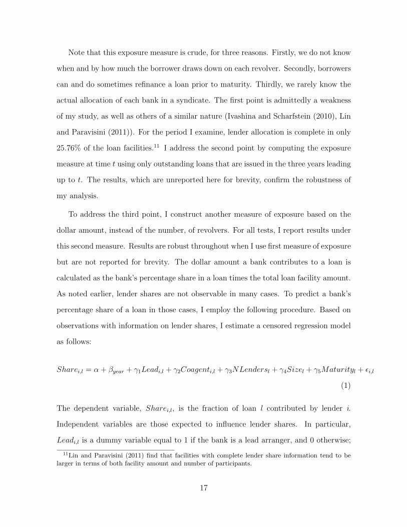
Note that this exposure measure is crude, for three reasons. Firstly, we do not know

when and by how much the borrower draws down on each revolver. Secondly, borrowers

can and do sometimes refinance a loan prior to maturity. Thirdly, we rarely know the

actual allocation of each bank in a syndicate. The first point is admittedly a weakness

of my study, as well as others of a similar nature (Ivashina and Scharfstein (2010), Lin

and Paravisini (2011)). For the period I examine, lender allocation is complete in only

25.76% of the loan facilities.11 I address the second point by computing the exposure

measure at time t using only outstanding loans that are issued in the three years leading

up to t. The results, which are unreported here for brevity, confirm the robustness of

my analysis.

To address the third point, I construct another measure of exposure based on the

dollar amount, instead of the number, of revolvers. For all tests, I report results under

this second measure. Results are robust throughout when I use first measure of exposure

but are not reported for brevity. The dollar amount a bank contributes to a loan is

calculated as the bank’s percentage share in a loan times the total loan facility amount.

As noted earlier, lender shares are not observable in many cases. To predict a bank’s

percentage share of a loan in those cases, I employ the following procedure. Based on

observations with information on lender shares, I estimate a censored regression model

as follows:

Sharei,l = α + βyear + γ1Leadi,l + γ2Coagenti,l + γ3NLendersl + γ4Sizel + γ5Maturityl + εi,l

(1)

The dependent variable, Sharei,l, is the fraction of loan l contributed by lender i.

Independent variables are those expected to influence lender shares. In particular,

Leadi,l is a dummy variable equal to 1 if the bank is a lead arranger, and 0 otherwise;

11Lin and Paravisini (2011) find that facilities with complete lender share information tend to belarger in terms of both facility amount and number of participants.

17

Coagenti,l is a dummy variable equal to 1 if the bank is a lead arranger, and 0 otherwise;

βyear is the year fixed effects; NLendersl is the number of lenders in facility l ; Sizel is the

log of the loan amount; and Maturityl is the loan’s maturity (the number of months

between the loan contractual start date and end date). I expect lenders with more

important roles to contribute a larger share, and lenders in larger syndicates (with a

higher number of members of a larger facility amount) to contribute a smaller share.

Finally, I expect lender shares to be smaller for longer maturity loans which tend to

involve higher risks. I then use the estimated coefficients from (1) to predict the lender

shares in cases where such information is not observed in Dealscan.12

Depth of Lender Roles

From the discussion in Section 2.1, I argue that more important (“deeper”) lender

roles are associated with higher future liquidity risk, the risk that the bank cannot

sell their share of the loan when they want to. To construct the Depth of Lender

Roles variables, I first assign lender roles based on information provided in Dealscan’s

LeadArrangerCredit and LenderRole fields. I identify a lender as a lead arranger if 1.

LeadArrangerCredit field indicates “Yes”; or, 2. The LeadArrangerCredit field indicates

“No” but “LenderRole” is one of the following: administrative agent, agent, arranger,

bookrunner, coordinating agent, lead arranger, lead bank, lead manager, mandated

arranger, and mandated lead arranger. I assign a lender the “co-agent” title if she

is not a lead arranger as determined from the above procedure and her “LenderRole”

is one of the following: co-agent, co-arranger, co-lead arranger, documentation agent,

managing agent, senior arranger, and syndication agent. A lender is also classified as a

co-agent if the LeadArrangerCredit field indicates “No” but her “LenderRole” falls in

12Main coefficient estimates (with t-statistics reported in parentheses) from estimating (1) are asfollows:

Sharei,l ≈ 99.8(205.75) + 15.767(211.73)Leadi,l + 3.02(38.80)Coagenti,l

+−0.281(−97.37)NLendersl +−4.42(−174.11)Sizel +−0.086(−69.56)Maturityl

All coefficients are as expected and significant at the 1% level.

18

the list of titles held by banks awarded a “Yes” in the LeadArrangerCredit field.

I employ three variables to proxy for the depth of lender roles. The first variable is

Role Depth, which is an ordinal variable taking the value of 1 if bank b is a participant

in loan l made to firm f , 2 if the bank is a co-agent, and 3 if it is a lead arranger (or

co-lead). Second is Lead, a dummy variable, which equals 1 if the bank is the lead (or

co-lead), and 0 otherwise. Finally, Important, is a dummy variable taking the value

of 1 if the bank is either a lead arranger (or co-lead) or a co-agent, and 0 otherwise.

Higher values for these variables indicate deeper lender roles.

Lender Distance

I hypothesize that post Lehman’s bankruptcy, banks that are more exposed to liquidity

problems via co-syndicating revolvers with Lehman should form more stable syndicates.

I argue that one way to do so is by diversifying lenders in terms of their borrower

pools. By choosing to syndicate with banks whose borrower pools are distant or less

correlated with their own, an exposed bank subject itself to a smaller risk that its

syndicate members may experience liquidity problems when the bank is also in trouble.

Reducing this risk is important, as banks do not want to face a greater draw-down rate

arising from the potential impairment of other syndicate members at a time when they

are experiencing liquidity problems. I adapt the “distance” variable proposed by Cai

et al. (2011) as a measure of lender diversification.

I define a bank’s measure of diversification in a syndicate as the average distance in

loan portfolios between the bank and other syndicate members. Calculating the distance

in loan portfolio holdings between two lenders involves the following steps. First, I need

to compute each lender’s portfolio weights in each industry category. For each lender

i - loan l combination, I search for all loans arranged by lender i in a lead arranger

role over the three-year period leading up to date t. The portfolio weight of lender i in

industry j at time t, denoted as wi,j,t is determined by dividing the dollar amount of

19

loans extended to firms belonging to industry j, over the total dollar amount of loans

the bank arranges as a lead lender.13 Note that∑J

j=1wi,j,t = 1, where J is the total

number of industries the lender can invest in. For the purpose of classifying borrower

industries, I follow Cai et al. (2011) and employ Standard Industry Classification (SIC)

1-digit and SIC 2-digit systems. In addition, to be consistent with the traditional asset

pricing literature, I adopt Fama and French (1994)’s 49 industry classification, which

is published on Kenneth French’s website.

The distance between the two lenders m and n in a syndicate formed at time t,

dm,n,t, is then simply the Euclidean distance in their weights in a J -dimensional space:

dm,n,t =

√√√√ J∑j=1

(wm,j,t − wn,j,t)2 (2)

which captures how similar syndicated loan portfolios are between two lenders.

Appendix A provides an example of how to calculate distance between two lenders.

Suppose that there are N syndicate members contributing to loan l, formed on

date t. Bank b’s lender diversification in syndicate l, denoted Db,l,t is computed as the

average distance between bank b and other syndicate members, calculated using all

loans originated by these lenders in lead arranger roles in the three-year period leading

up to date t :

Db,l,t =

(∑N−1n=1 dbn,memn,t

)N − 1

(3)

where dbn,memn,t denotes the distance between the nth pair of bank b and syndicate

member memn, and bn 6= memn.

13where a syndicate consists of more than one lead arranger, I divide the facility amounts equallyamong the lead banks.

20

3.3 Summary Statistics

In this section, I describe my main sample, which includes revolvers originated by

bank-firm pairs that exist both before and after Lehman’s collapse. In Table 1, I

partition this sample into two sub-samples, corresponding the pre-event (June 1, 2005

to September 14, 2008) and post-event (September 15, 2008 to December 31, 2009)

periods. The average bank has $741 million in assets pre-Lehman, which increases to

$948 million post-Lehman. This increase reflects the many mergers that happened over

the sample period. As expected, banks’ performance deteriorated in the post-Lehman

period, evidenced by a decrease in ROA and capital ratios and an increase in loan loss

ratios. The ratio of core deposits over total assets, however, increases, reflecting either

a flight to quality or banks’ efforts to adjust their balance sheets (see Acharya and

Mora (2012)). My measure of exposure to Lehman revolvers decreases post-Lehman,

reflecting the maturity of certain Lehman-cosyndicated revolvers.

Borrowing firms also experience performance deterioration in the post-event period.

Their sales, interest coverage ratios and net working capital drop and their leverage

increases. The fraction of tangible assets, however, remains unchanged over the sample

period. With liquidity being dried up and the poor performance of banks during the

crisis, the terms of revolvers’ contracts became worse as expected. As can be seen from

Panel C of table 1, the average all-in-drawn spread increases, and the facility amount

and maturity both decrease post-Lehman.

Are banks with high exposure to Lehman revolvers different from those with low

exposure? Cosyndicating with Lehman is clearly a bank’s choice variable. As a result,

it is important to understand how exposure may correlate with observable bank charac-

teristics. In the first two columns of Table 2, I break out my sample in the pre-Lehman

period (June 1, 2005 to September 14, 2008) into two groups: banks with no exposure

to Lehman (23 banks) and those with positive exposure (27 banks). It is noticeable that

21

exposed banks are much larger and more risky compared to their non-exposed coun-

terparts: they have fewer core deposits and are funded by more subordinated debt.

Nonetheless, they do not differ in terms of various performance measures such as ROA,

capital and loan loss ratios. Exposed banks also lend to larger, older firms with lower

interest coverage ratios. They also participate in closer/less distant syndicates. Finally,

exposed banks lend on better terms with lower all-in-drawn spreads and larger facility

sizes.

I then focus on exposed banks only and examine differences in bank characteristics,

borrower pools, and loan characteristics between the high-exposure and low-exposure

groups. The high-exposure group consists of the fourteen top exposure banks, and

the low-exposure group is made up of the remaining thirteen banks. Here the high

and low exposure groups do not differ very much. High-exposure banks, on average,

are still larger. But the statistical significance is only at the 10% level. Furthermore,

bank performance and risk measures (ROA, core deposits, subordinated debt, capital,

and loan loss ratios) are economically and not statistically different among the two

groups. On the other hand, they are still different in terms of borrower pool and loan

characteristics, with high-exposure banks extending less expensive and larger loans to

larger, more older firms with fewer tangibles. However, the syndicates formed by high

and low exposure banks are not different in the measure of facility distance.

Given differences among banks with different exposure to Lehman revolvers, one is

concerned about a classic endogeneity issue. That is, the collapse of Lehman Brothers

may affect risk-sharing incentives of banks via characteristics that are correlated with

exposure. If this were the case, any effect found on exposure could merely be correlation,

and not causation. I address this concern in two ways. First, I control for bank and

borrower characteristics in all my regressions. Second, as noted above, most differences

in lender characteristics are found between exposed and non-exposed banks, rather than

22

between high-exposure and low-exposure banks. Therefore, in one of the robustness

tests, I exclude the 23 banks that do not have any exposure during the sample period.

I argue that exclusion of these banks does not cause serious sample selection bias, as

they are far less frequent players in the syndicated loan market when compared to

exposed banks. In fact, the 23 non-exposed banks participate in only 78 revolvers in

the pre-event period, compared to 931 co-syndicated by the 27 exposed banks.

Differences in borrower characteristics for loans made by banks with different ex-

posure levels raise a further concern that a credit demand shock post-Lehman that is

correlated with bank exposure might have led to the observed outcome. Specifically,

if more exposed banks lend to worse quality borrowers, who suddenly became much

riskier following Lehman’s collapse, then findings that exposed banks reduce the signif-

icance of their role and form more diversified syndicates might be driven by a demand

side effect. Panel B and C of Table 2 shows that this is not the case. If anything, more

exposed banks lend to safer and more established firms: their customers are larger,

older and have fewer tangibles.

4 Empirical Methodology and Results

4.1 Bank Lending Channel

In this section, I revisit the “bank lending channel” hypothesis. In particular, I exam-

ine how bank exposure to liquidity risk affects (i) lending activity and (ii) other loan

contract terms. To investigate (i), I start with the following specification:

∆Lendingb = α + βExposure LEHb + ρ′∆Xb + εb (4)

23

The dependent variable, ∆Lendingb, is the change in the logs of bank lending activity in

the pre- and post- Lehman’s bankruptcy periods, which correspond to the 365 days be-

fore and after September 15, 2008. I measure lending activity for a bank in each of these

two periods as the total number of loan facilities in which the bank participates. The

main explanatory variable of interest, Exposure LEHb, is bank b’s exposure to Lehman

co-syndicated revolvers, as defined in Section 3.2, and measured as of September 15,

2008. The coefficient of interest, β, measures the impact of this exposure on the change

in bank lending activity. ∆Xb is a vector of changes in bank control variables, where

changes are measured by the quarterly average of these variables in the post-Lehman

period, minus the corresponding value in the pre-Lehman period. Bank controls in-

cluded in Xb are: Log assetsb, Core Depositsb, ROAb, Loan lossb, and Capital Ratiob.

I expect larger banks to be better diversified and less risky. Hence they can afford to

pass on more favorable terms to the borrowers. A similar argument goes for banks with

a high ratio of core deposits, which are usually considered to have a more stable source

of funding. Finally, better performing banks, those with higher ROA, higher capital

ratios and smaller loan losses are expected to be more healthy and can lend on better

terms.

Column 1 of Table 3 presents the results estimating regression (4). We can see that

on average, banks reduced their lending activity in half following Lehman’s collapse.

Consistent with the result in Ivashina and Scharfstein (2010), banks that are more

exposed to liquidity risk via co-syndicating revolvers with Lehman reduced their lending

by more than less exposed banks. The effect is both statistically and economically

significant. A one standard deviation (3.944%) increase in Exposure LEH is associated

with a 16.17% decrease in new loan originations. When I break out lending activity

into that related to revolvers and term loans (Columns 2 and 3 of Table 3), the effect

is concentrated in the revolver sample only. In the term loan sample, β is still negative

24

but is no longer statistically significant. This result is consistent with Irani (2012), who

finds that a negative shock to bank health affects its lending, but that this effect is more

pronounced in banks’ liquidity provision via revolvers relative to their credit provision

via term loans.

The disadvantage of estimating (4) is that it ignores borrower characteristics and

therefore does not take into account the possible effect of a credit demand shock. This is

a concern if (i) there are differences in characteristics between firms that did and did not

take out loans following Lehman’s collapse, and (ii) these characteristics are correlated

with the Exposure LEH variable in the cross section. To alleviate this concern, I focus

on loan level analysis in the rest of the paper, and only examine loans that are taken

out by the same firms from the same banks before and after Lehman’s collapse. The

regression specification is as follows:

Termsb,f,l,t =αb,f + δSIC + β1Postt + β2Exposure LEHb,t

+ β3Exposure LEHb,t ∗ Postt + γ′Xb,t + ρ′Zf,t + εb,f,l,t (5)

The coefficient of interest is β3, which measures the differential effect of the change in

exposure on lending terms in the post Lehman period, between high- and low-exposure

banks. Loan contractual terms I consider, Termsb,f,l,t, include maturity, all-in-drawn-

spread, and (the log of) facility size attached to revolver l, made to firm f by bank b at

time t. αb,f denotes bank-firm fixed effects. δSIC denotes industry fixed effects. Postt

is a dummy variable equal to 1 if the loan is made in the post-Lehman period; and

0 otherwise. Exposure LEHb,t is bank b’s exposure to Lehman co-syndicated revolvers

measured at time t, as defined in Section 3.2. Xb,t and Zf,t are, respectively, vectors of

bank and firm control variables, which are defined in Table B-2. All control variables

are measured in the quarter immediately prior to the loan origination date t.

25

Bank controls, Xb,t, are previously defined. Firm controls, Zf,t, include Log Salesf,t,

Leveragef,t, Interest Coveragef,t, Net Working Capitalf,t, Tangiblesf,t, Firm Agef,t and

Investment Gradef,t. I expect larger and older firms to be more established and less

risky, and thus are able to obtain more favorable terms. Firms with high leverage and

low interest coverage are riskier and hence are expected to borrow on worse terms.

Firms with less net working capital and more tangibles tend to lose more value in

default, thus have higher default risk and command worse borrowing terms. Finally,

investment grade firms are better credits and thus should command more favorable

terms.

Including time-varying observable and unobservable bank and firm control variables

is important in explaining loans’ contract terms. Nonetheless, I continue to worry about

unobservables that may drive (i) the sample selection of borrowing firms in the post-

event period; and (ii) the matching between banks and firms. In particular, (i) relates

to the concern that there may be unobservable differences between firms that decide

to borrow in the post-Lehman period and firms that do not. On the other hand, (ii)

relates to the concern that firms with certain characteristics are likely to borrow from

banks with characteristics that are correlated with the exposure variable.

To address these issues, I only include in my sample firm-bank pairs that have re-

volver contracts with each other both in the pre- and post-Lehman periods, and employ

bank-firm fixed effects in the regression. This way, β3 is identified only from the inten-

sive margin of lending. In other words, it is identified from changes in the dependent

variable within relationship, one that is established by the same firm borrowing from

the same bank both before and after the event. This approach closely follows previous

work in the literature examining syndicated lending (see, for example, Glenn Hubbard

and Palia (2002), Lin and Paravisini (2011), Irani (2012), and Santos (2011)). It ad-

dresses (i) by excluding firms that do not borrow following the event. In addition, it

26

addresses (ii) by taking away the cross-sectional mean of characteristics that influence

firm-bank matching, leaving the effect of exposure to be identified from between-bank

variation at a given point in time.

Note that although estimators from within-relationship estimation are consistent,

results cannot be extrapolated to the extensive margin of lending. That is, we do not

know whether or how banks’ and firms’ exiting relationships continue to lend and borrow

after the shock. This is a common limitation applying to within-relationship estimators

(see Lin and Paravisini (2011), Khwaja and Mian (2005), and Schnabl (2012)). Finally,

I follow Petersen (2009) and cluster standard errors by both firm and bank. This

allows for the fact that the error components of lending policies in regression (5) may

be correlated across banks lending to the same firm, and across firms for loans made by

the same bank. Clustering by both the bank and firm dimensions are important, for two

reasons. First, because the shock happens at the bank level, changes in lending policies

may be correlated among loans originated by the same bank. Second, a firm receives

multiple loans over the sample period, changes in contractual terms from different banks

may be correlated within the same firm.

Table 4 shows the results estimating regression (5) on maturity, all-in-drawn spread

and facility size for my sample of revolvers. All else equal, an average bank in the sample

does not alter their maturity and facility size following Lehman’s collapse. However,

they do charge larger spreads, reflecting the overall liquidity crisis. Interestingly, more

exposed banks reduce the maturity of revolvers they syndicate following Lehman’s

collapse, relative to less exposed banks. The estimated coefficient of interest, β3, is

negative and statistically significant. A one standard deviation difference in exposure

translates to a difference in the pre-Lehman - post-Lehman change in maturity of 3.9

months. There is no statistical difference in changes in spread and facility size between

exposed and non-exposed banks.

27

How does this result reconcile with results in Table 3 and in Ivashina and Scharf-

stein (2010) who find that banks that are more exposed to liquidity problems lend less

during the 2007-2009 financial crisis? Note that in testing specification (5), I look ex-

clusively at the intensive lending margin. It is entirely possible that on aggregate, more

exposed banks lend less post-Lehman, but for those borrowers to whom they continue

to lend, they do not reduce the facility size. This is indeed what Irani (2012) finds while

examining the impact of bank health on corporate liquidity provision.

I now turn to examine the main question of this study. If exposed banks do not

worsen the terms of lending, do they structure their syndicates in a way that reduce

future risks? In particular, do they participate in less important roles following the

shock? If they remain as the lead arranger (or co-lead), do they choose to form more

stable syndicates?

4.2 Change in Depth of Syndicate Roles

4.2.1 Exposed Banks Reduce the Depth of Their Roles

In this section, I examine how exposure to liquidity risk leads to banks changing the

depth of their syndicate roles. The regression specification is the same as (5), except

that the dependent variable is now Role Importanceb,f,l,t, the importance of the role

played by bank b, in revolver l made to firm f at time t:

Role Importanceb,f,l,t =αb,f + δSIC + β1Postt + β2Exposure LEHb,t

+ β3 ∗ Exposure LEHb,t ∗ Postt + γ′Xb,t + ρ′Zf,t + εb,f,l,t (6)

Three variables measuring the Role Importance are used: (1) Role Depthb,f,l,t, an

ordinal variable taking the value of 1 if bank b is a participant in loan l made to firm

f , 2 if the bank is a co-agent, and 3 if it is a lead arranger (or co-lead); (2) Leadb,f,l,t,

28

a dummy variable, which equals 1 if the bank is the lead (or co-lead), and 0 otherwise;

and (3) Importantb,f,l,t, a dummy variable taking the value of 1 if the bank is either a

lead arranger (or co-lead) or a co-agent, and 0 otherwise. All other variables are defined

in section 4.1. Again, the unit of observation here is a bank-firm-loan triple.

Results of testing this change in banks’ syndicate roles are reported in the first three

columns of Table 5. Column (1) suggests that more exposed banks are more likely to

reduce the depth of their role following Lehman’s bankruptcy. The coefficient on the

interaction term, Exposure LEHb,t ∗ Postt is negative and statistically significant. The

magnitude of the coefficient suggests that a one standard deviation increase in exposure

leads to a decrease of -0.149 units of the depth of role. Given that banks rarely change

the depth of their role for the same borrower (the average and median bank level

change in the depth of role across all revolvers in the post-Lehman period is 0.015 and

0 respectively), this effect is economically significant.

Given that more exposed banks are more likely to play a less important role in a

syndicate in the post-Lehman period, I next examine which type of role they find it

easier to switch away from. In column (2), I examine the impact of exposure on a

bank’s decision to participate as a lead arranger. Again, I find that banks with higher

exposure to Lehman revolvers are less likely to participate as a lead arranger following

Lehman’s collapse. However, while the estimated β3 is negative, it is not statistically

significant. As relationship lending is formed at the lead arranger level, these results

suggest that lending relationship is sticky, i.e., lead arrangers who continue to fund a

relationship borrower’s loan after the shock do not forgo their lead-arranging role.

On the other hand, when the depth of syndicate role is proxied for by whether the

bank is a key lender (either lead arranger or co-agent), I continue to find the risk-

sharing result. That is, more exposed banks are more likely to join the syndicate as a

participant following Lehman’s collapse. Column (3) shows a negative and statistically

29

significant estimate for β3. In terms of economic significance, a one standard deviation

increase in exposure results in an 11.5% decrease in the probability that the bank joins a

syndicate as a key lender in the post-Lehman period. This result is consistent with the

hypothesis that higher exposure leads to banks willing to share less risk in a syndicate.

Specifically, they are more likely to be in participant roles, such that they can more

easily sell off the loan when illiquidity becomes imminent.

One could argue that a decrease in role depth has nothing to do with risk-sharing.

But rather, the same bank lending channel as in Ivashina and Scharfstein (2010) could

be at work. In other words, more exposed banks could merely reduce their allocation

to a syndicate following Lehman’s collapse, and thus were given less important roles.

I address this concern in two ways. Firstly, I show in Section 4.1 that more exposure

does not lead to a decrease in the size of the facility. This test is, however, crude as it

looks at the effect of exposure on the total facility size rather than banks’ individual

commitments. Therefore, I restrict my sample to only bank-firm-loan observations

where information on bank allocation is not missing. Using this sample to analyze the

effect of exposure on individual banks’ contribution, I find the coefficient of interest,

β3, to be indistinguishable from zero. 14

Second, I show that the same syndicate role adjustments do not happen for term

loans. I expect that risk-sharing adjustments in anticipation of liquidity shocks would

arise more in revolvers than in term loans. While the latter represents up-front com-

mitments and involves only credit risk from the borrower, the former entails both credit

risk and liquidity risk. Consistent with this argument, columns (I)-(III) of Table B-3

show that the coefficient of interest is not statistically significant under any definition

of syndicate role depth. Moreover, it turns positive for specifications where Lead or

Role Depth are dependent variables.

14Results from this test are unreported in this paper, but are available upon request.

30

4.2.2 Risky Borrowers

The previous section shows that more exposed banks, in an effort to reduce liquid-

ity risks associated with revolver commitments, take on less important roles following

Lehman’s collapse. A natural question then arises: do these adjustments depend on

borrower characteristics? In other words, do banks actively manage their risk-sharing

arrangements more for borrowers who pose a greater liquidity concern?

I define borrowers that pose a greater liquidity concern as those having a non-

investment grade credit rating. Non-investment grade borrowers are considered worse

credits, who are less likely to have access to alternative sources of funding when their

relationship lender runs into trouble. As a result, they are more likely to draw down on

banks’ credit lines for precautionary purposes. As such, I hypothesize that incentives for

risk-sharing adjustments should be more intense for non-investment grade borrowers,

relative to investment-grade ones.

To test this hypothesis, I employ Dealscan’s investment-grade classification and

break out the main sample into two subsamples: investment-grade and non-investment

grade borrowers. I rerun regression (6) separately on these two subsamples, and com-

pare the coefficient on Exposure LEHb,t ∗ Postt between them. For all regressions, I

employ both measures of exposure based on the number (Panel A), and dollar amount

(Panel B) of revolver exposure to Lehman respectively, and confirm that the conclu-

sions are the same under both measures. The results, presented in Table 6, show that

risk-sharing adjustments by exposed banks are primarily concentrated in the sample of

risky borrowers. In particular, the first two columns (I and II), which seek to explain

a bank’s depth of role, reveals a negative coefficient on Exposure LEHb,t ∗ Postt for

both sub samples. However, the magnitude of such a coefficient is five times larger for

non investment-grade borrowers. Furthermore, while the effect is strongly statistically

significant for these borrowers, it is no longer significant for investment-grade borrowers.

31

A similar pattern emerges when examining a bank’s decision to be an impor-

tant lender (“Important”) as we see in columns IV and V. Here, the coefficient on

Exposure LEHb,t ∗Postt is ten times greater in magnitude for the non-investment grade

subsample, compared to the investment-grade one. As a robustness test, I estimate a

pooled regression for the entire sample, and interact Exposure LEHb,t ∗ Postt with the

Investment Grade dummy variable (columns III and VI). As can be seen, the coefficient

on the triple-interaction variable is positive, and highly significant in the case where

Important is the dependent variable. Overall, the results suggest that banks do actively

manage their risk-sharing capacity via adjusting their roles. Moreover, they are more

likely to do so when the borrowers pose greater liquidity risks.

4.3 Syndicate Diversification

4.3.1 Exposed Lead Banks Choose More Distant Members

Results in Section 4.2 indicate that lead arranging roles are not affected by banks’

exposure in a significant way. If relationships are sticky and lead banks cannot offload

liquidity risk by reducing the depth of their role, do they structure their syndicates in a

way that reduces their exposure to future liquidity risk? Here I argue that exposed lead

banks are likely to form more diversified syndicates by choosing more distant co-lenders

following the shock. Choosing more distant co-syndicators benefits the exposed lead

arranger, as she is less likely to take on additional liquidity risk arising from the default

of other syndicate members when she is also in trouble.

To examine this diversification hypothesis, I employ a modified version of specifica-

32

tion (5), as follows:

Db,f,l,t =αb,f + SICf + β1Postt + β2Exposureb,t + β3 ∗ Exposureb,t ∗ Postt

+ β4 ∗ Leadb,f,l,t + β5 ∗ Leadb,f,l,t ∗ Postt + β6 ∗ Leadb,f,l,t ∗ Exposureb,t (7)

+ β7 ∗ Leadb,f,l,t ∗ Exposureb,t ∗ Postt + γ′Xb,t + ρ′Zf,t + εb,f,l,t

The dependent variable, Db,f,l,t, is a measure of distance between bank b and other

syndicate members (“syndicate diversification”), defined in Section 3.2. The coefficient

of interest is now that on the triple interaction variable, β7, which measures the effect

of the lead arranger’s exposure on syndicate diversification following the shock.

The results examining this hypothesis is presented in Table 7. Distance is measured

based on borrower SIC 1-digit (i), SIC 2-digit (ii), and Fama and French’s 49 industry

classification (iii). The first three columns estimate the average effect of exposure on

distance for all syndicate participants, regardless of what role they take. The estimated

coefficient of interest is positive, consistent with the hypothesis that more exposed

banks forms more distant syndicates. The effect, however, is not statistically robust

across measures of distance. While it is significant at the 5% level for measure (i), it

is only weakly significant at the 10% level for measure (iii) and no longer retains its

significance for measure (ii).

This is not surprising since not all syndicate members’s exposure levels are expected

to affect their incentives to diversify with respect to co-syndicators. It is the lead ar-

ranger whose diversification concern is the biggest. First, as shown in Section 4.2,

compared to coagents, exposed lead arrangers do not have much option to limit their

risk by taking on less important roles and hence would find lender diversification as

a possible alternative. Second, lead arrangers usually contribute a significant amount

to a syndicated loan, thereby subjecting themselves to a significant liquidity shock

when other members are unable to honor their commitments. Therefore, I estimate

33

specification (7), focusing on the coefficient of interest, β7. The results are provided

in columns (4) and (5), and (6) of Table 7. As can be seen, β7 is positive and sta-

tistically significant. This suggests that more exposed lead banks form more distant

syndicates following the shock. The effect is highly economically significant: for exam-

ple, when syndicate distance is measured based on borrower 1-digit SIC classification, a

one standard deviation increase in the lead bank’s exposure leads to 0.07 units increase

in lender distance (which is equal to about 17% of the sample average). Again, this

result is not obtained with the term loan sample, where the estimated coefficient of

interest is indistinguishable from zero (See columns (IV), (V), and (VI) of Table B-3).

4.3.2 Syndicate Diversification: What Type of Lenders Matters?

Given that more exposed lead banks want to form syndicates with more “distant”

members, I now examine with which members the lead arranger’s diversification con-

cern is the greatest. Arguably, compared to participants, co-leads and co-agents are

more important members who usually contribute a bigger share to a loan and thereby

causing greater liquidity problems for the lead arranger should they default. As such, I

expect the lead bank’s diversification concern with respect to these important lenders

should dominate that with respect to members with participant roles. To examine this

hypothesis, I reconstruct a bank’s distance measure (i) as the average distance between

the bank and other important members; and (ii) as the average distance between the

bank and participants only. I rerun regression (7) for distance measures (i) and (ii) and

report the results in Panels A and B of Table 8, respectively.

Panel A shows that more exposed lead banks form syndicates with more distant im-

portant lenders, following Lehman collapse. The coefficient on Leadb,f,l,t ∗Exposureb,t ∗

Postt is positive and highly statistically significant. A positive coefficient of interest

is also found in Panel B, where the distance measure is calculated between the bank

34

and syndicate participants. However, it is no longer statistically significant, even at the

10% level. The results suggest that an exposed lead bank has diversification concern

in mind when choosing important syndicate members but not when choosing members

with participant roles.

5 Robustness

5.1 Logit Regressions

So far, regressions involving measures of the significance of syndicate roles as dependent

variables are estimated using linear probability models. While being consistent in the

presence of fixed effects, these models produce estimates that imply probabilities outside

the [0,1] range. In Panel A of Table 9, I repeat these analyses using conditional logit

models for Lead and Important, and conditional ordinal logit model for Role Depth,

with the same set of control variables and fixed effects as in (5). As can be seen, the

results are qualitatively similar to those under linear probability models. Noticeably,

the estimated coefficient on Exposure LEHb,t ∗ Postt in the Lead regression is now

statistically significant. As logit regressions with many fixed effects may suffer from

the incidental parameter problem (e.g. Greene (2004)), all inferences in this paper are

made with reference to results from linear probability models.

5.2 Removing Banks with Zero Exposure

As discussed in Section 3.3, non-exposed banks are remarkably different from exposed

banks along several dimensions. In Panel B of Table 9, I show that the main risk-

sharing results are robust to the exclusion of non-exposed banks. In particular, the

coefficient estimates are essentially the same as those from original tests, both in eco-

nomic magnitude and statistical significance. Section 3.3 also shows that conditioning

35

on being exposed, banks with high and low exposure levels do not differ from each other

except in banks’ asset size. In unreported results, I interact bank size with Postt in all

regressions and confirm that the main results remain the same qualitatively.

5.3 Pre-exsiting Trend

One important concern with my empirical strategy is that the results might purely pick

up a trend in the data that is unrelated to banks’ liquidity risk arising from revolver

draw-down post Lehman bankruptcy. For example, there might be some time-invariant

characteristics of the data which induce more exposed banks to decrease the depth of

their role over time, relative to less exposed ones. In order to address this concern, I

perform a set of “placebo” tests, where I move the event date to June 15, 2007, and the

sample period from March 15, 2004 to September 14, 2008.15 If the same results in the

original tests are found in this “placebo” sample, my results would be unconvincing.

Panel C of table 9 reports the results of these tests, which confirms absence of a

pre-existing trend. In particular, the coefficient on Exposure LEHb,t ∗ Postt switches

its sign and becomes positive in tests on changes in lender roles. The coefficient on

Leadb,f,l,t ∗Exposureb,t ∗Postt turns negative, indicating that more exposed lead banks

are more likely to keep closer syndicates in the “post-event” period. All coefficients of

interest are, however, now statistically indistinguishable from zero.

6 Concluding Remarks

I provide evidence that banks actively manage their risk-sharing arrangements in syndi-

cated revolving lines of credit when facing liquidity risk. Using the collapse of Lehman

Brothers as a shock to bank liquidity risk exposure arising from undrawn revolvers, I

15The decision about the “placebo” date and sample period is to ensure I have the same number ofmonths pre- and post-event as in the original tests.

36

examine how risk-sharing arrangements alter among banks with different levels of ex-

posure to the shock. The syndicate structure of multiple participants provides a useful

setting to identify this exposure, as different banks have different direct exposure via

their level of co-syndication with Lehman.

I exclusively examine this question at the intensive lending margin, i.e., I look only

at firms that borrow from the same banks both before and after the crisis. Looking

within-relationship allows me to control for factors that influence the lender-borrower

match, and help me abstract from confounding factors that might affect the relationship

exit decisions. I find that exposed banks that continue to lend to the same firm do not

worsen the rates charged or reduce the amount of commitment relative to other banks,

following the shock. However, the results suggest that they were able to do so thanks

to active management of risk-sharing arrangements. More exposed banks that join

revolver syndicates do so in less important roles. Banks that stay as lead arrangers to

the same firm form more diversified syndicates. These risk-sharing adjustments would

help lenders limit their exposure to future liquidity shocks.

In this paper, I have focused on US commercial banks only. It would be inter-

esting to extend this study to other types of financial institutions that participate in

the syndicated loan market. Some preliminary analyses reveal that risk-sharing ad-

justments following Lehman’s collapse are more concentrated in non-commercial-bank

institutions. This could be further evidence suggesting the advantage of commercial

banks in providing liquidity.

37

References

Acharya, V. V. and Mora, N. (2012). Are banks passive liquidity backstops? deposit

rates and flows during the 2007-2009 financial crisis. NYU Working Paper.

Ball, R., Bushman, R. M., and Vasvari, F. P. (2008). The debt-contracting value of

accounting information and loan syndicate structure. Journal of Accounting Research,

46(2):247–287.

Cai, J., Saunders, A., and Steffen, S. (2011). Syndication, interconectedness, and

systemic risk. Working paper, NYU Stern School of Business, (5).

Chava, S. and Roberts, M. R. (2008). How does financing impact investment? the role

of debt covenants. The Journal of Finance, 63(5):2085–2121.

Cornett, M. M., McNutt, J. J., Strahan, P. E., and Tehranian, H. (2011). Liquidity risk

management and credit supply in the financial crisis. Journal of Financial Economics,

101(2):297 – 312.

Dennis, S. A. and Mullineaux, D. J. (2000). Syndicated loans. Journal of Financial

Intermediation, 9(4):404 – 426.

Diamond, D. W. (1984). Financial intermediation and delegated monitoring. The

Review of Economic Studies, 51(3):393–414.

Diamond, D. W. and Dybvig, P. H. (1983). Bank runs, deposit insurance, and liquidity.

Journal of Political Economy, 91(3):401–419.

Esty, B. C. and Megginson, W. L. (2003). Creditor rights, enforcement, and debt

ownership structure: Evidence from the global syndicated loan market. Journal of

Financial and Quantitative Analysis, 38(1):37–60.

38

Fama, E. and French, K. (1994). Industry cost-of-equity capital. Working Paper,

University of Chicago and Yale University.

Gatev, E. and Strahan, P. E. (2009). Liquidity risk and syndicate structure. Journal

of Financial Economics, 93(3):490 – 504.

Glenn Hubbard, K. K. and Palia, D. (2002). Are there bank effects in borrowers’

costs of funds? evidence from a matched sample of borrowers and banks. Journal of

Business, 75(4):559–581.

Greene, W. (2004). Fixed effects and bias due to the incidental parameters problem in

the tobit model. Econometric Reviews, 23(2):125–147.

Holmstrom, B. (1979). Moral hazard and observability. The Bell Journal of Economics,

10(1):pp. 74–91.

Holmstrom, B. and Tirole, J. (1997). Financial intermediation, loanable funds, and the

real sector. The Quarterly Journal of Economics, 112(3):663–691.

Irani, R. (2012). Bank health and corporate liquidity provision. Working Paper, Uni-

versity of Illinois at Urbana Champagne.

Ivashina, V. (2009). Asymmetric information effects on loan spreads. Journal of Fi-

nancial Economics, 92(2):300 – 319.

Ivashina, V. and Scharfstein, D. (2010). Bank lending during the financial crisis of

2008. Journal of Financial Economics, 97(3):319 – 338.

Ivashina, V. and Sun, Z. (2011). Institutional stock trading on loan market information.

Journal of Financial Economics, 100(2):284 – 303.

Jones, J. D., Lang, W. W., and Nigro, P. J. (2005). Agent bank behavior in bank loan

syndications. Journal of Financial Research, 28(3):385–402.

39

Kashyap, A. K., Rajan, R., and Stein, J. C. (2002). Banks as liquidity providers:

An explanation for the coexistence of lending and deposit-taking. The Journal of

Finance, 57(1):33–73.

Khwaja, A. I. and Mian, A. (2005). Do lenders favor politically connected firms? rent

provision in an emerging financial market. The Quarterly Journal of Economics,

120(4):1371–1411.

Lee, S. W. and Donald (2004). Monitoring, financial distress, and the structure of

lending syndicates. Financial Management, 33(3):107–130.

Leland, H. E. and Pyle, D. H. (1977). Informational asymmetries, financial structure,

and financial intermediation. The Journal of Finance, 32(2):371–387.

Lin, C., Ma, Y., Malatesta, P., and Xuan, Y. (2012). Corporate ownership structure

and bank loan syndicate structure. Journal of Financial Economics, 104(1):1 – 22.

Lin, H. and Paravisini, D. (2011). What’s bank reputation worth? the effect of fraud

on financial contracts and investments. Columbia Working Paper.

Petersen, M. A. (2009). Estimating standard errors in finance panel data sets: Com-

paring approaches. Review of Financial Studies, 22(1):435–480.

Santos, J. (2011). Bank corporate loan pricing following the subprime crisis. Review of

Financial Studies, 24(6):1916–1943.

Schnabl, P. (2012). The international transmission of bank liquidity shocks: Evidence

from an emerging market. The Journal of Finance, 67(3):897–932.

Sufi, A. (2007). Information asymmetry and financing arrangements: Evidence from

syndicated loans. The Journal of Finance, 62(2):629–668.

40

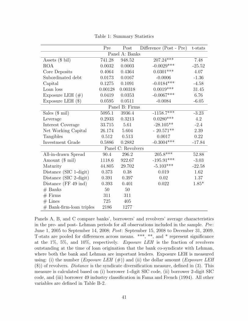
Table 1: Summary Statistics

Pre Post Difference (Post - Pre) t-statsPanel A: Banks

Assets ($ bil) 741.28 948.52 207.24*** 7.48ROA 0.0032 0.0003 -0.0029*** -25.52Core Deposits 0.4064 0.4364 0.0301*** 4.07Subordinated debt 0.0173 0.0167 -0.0006 -1.36Capital 0.1275 0.1091 -0.0184*** -4.58Loan loss 0.00128 0.00318 0.0019*** 31.45Exposure LEH (#) 0.0419 0.0353 -0.0067*** 6.76Exposure LEH ($) 0.0595 0.0511 -0.0084 -6.05

Panel B: FirmsSales ($ mil) 5095.1 3936.4 -1158.7*** -3.23Leverage 0.2933 0.3213 0.0280*** 4.2Interest Coverage 33.715 5.61 -28.105** -2.4Net Working Capital 26.174 5.604 - 20.571** 2.39Tangibles 0.512 0.513 0.0017 0.22Investment Grade 0.5886 0.2882 -0.3004*** -17.84

Panel C: RevolversAll-in-drawn Spread 90.4 296.2 205.8*** 52.88Amount ($ mil) 1118.6 922.67 -195.91*** -3.03Maturity 44.805 29.702 -5.103*** -22.58Distance (SIC 1-digit) 0.373 0.38 0.019 1.62Distance (SIC 2-digit) 0.391 0.397 0.02 1.37Distance (FF 49 ind) 0.393 0.401 0.022 1.85*# Banks 50 50# Firms 311 311# Lines 725 405# Bank-firm-loan triples 2186 1277

Panels A, B, and C compare banks’, borrowers’ and revolvers’ average characteristicsin the pre- and post- Lehman periods for all observations included in the sample. Pre:June 1, 2005 to September 14, 2008; Post : September 15, 2008 to December 31, 2009.T-stats are pooled for differences across means. ***, **, and * represent significanceat the 1%, 5%, and 10%, respectively. Exposure LEH is the fraction of revolversoutstanding at the time of loan origination that the bank co-syndicate with Lehman,where both the bank and Lehman are important lenders. Exposure LEH is measuredusing: (i) the number (Exposure LEH (#)) and (ii) the dollar amount (Exposure LEH($)) of revolvers. Distance is the syndicate diversification measure, defined in (3). Thismeasure is calculated based on (i) borrower 1-digit SIC code, (ii) borrower 2-digit SICcode, and (iii) borrower 49 industry classification in Fama and French (1994). All othervariables are defined in Table B-2.

41

Table 2: Exposure and Pre-Lehman Sample Characteristics

Exp (I) Non-Exp (II) (I)-(II) t-stat High Exp (III) Low Exp(IV) (III)-(IV) t-stat

Pabel A: Banks

Assets ($ bil) 274.44 24.05 250.39** -2.58 438.74 96.45 342.29* 1.85ROA 0.003 0.003 0 0.37 0.003 0.003 0 -0.02Core Deposits 0.37 0.594 -0.226*** -4.15 0.322 0.422 -0.1 -1.08Subordinated debt 0.019 0.008 0.011*** 2.9 0.018 0.02 -0.002 -0.18Capital 0.178 0.098 0.08 1.62 0.184 0.17 0.014 0.14Loan loss 0.0014 0.0009 0.0005 0.99 0.0017 0.0011 0.0006 0.63

Panel B: Firms

Sales ($ mil) 5302.5 935.7 4366.8*** 3.94 6208.9 2318.2 3890.7*** 6.73Leverage 0.294 0.289 0.005 0.89 0.295 0.289 0.006 0.67Interest Coverage 30.6 100.7 -70.1** -2.11 29.193 35.312 -6.119 -0.4Net Working Capital 26.872 10.762 16.11 0.5 28.348 21.932 6.416 0.39Tangibles 0.494 0.642 -0.148*** 6.51 0.482 0.538 -0.057*** -4.85Firm Age 25.725 20.654 5.071*** 3.41 26.107 24.467 1.65** 2.13

Panel C: Revolvers

All-in-drawn Spread 88.328 129 -40.682*** -4.81 82.891 105.5 -22.563*** -5.11Amount ($ mil) 1151.4 461.2 690.2*** 3.42 1319 599 720*** 6.83Maturity 44.825 44.398 0.427 0.2 44.56 45.7 -1.14 -1.06Distance (SIC 1-digit) 0.358 0.715 -0.358*** 26.3 0.334 0.431 -0.093*** -16.33Distance (SIC 2-digit) 0.377 0.744 -0.365*** -24.55 0.351 0.453 -0.098 -15.68Distance (FF 49 ind) 0.377 0.75 -0.37 -25.16 0.352 0.455 -0.1 -16.14

# Banks 27 23 14 13# Firms 347 47 322 149# Facilities 931 78 871 292

This table reports pre-Lehman banks’, borrowers’ and loans’ characteristics for banks with different exposure to Lehman’srevolving lines of credit. The sample includes revolvers originated over the period from June 1, 2005 to September 14, 2008.Exp (I)/Non-Exp (II) denotes the sample of banks that have positive/zero exposure to Lehman revolvers in the post Lehmanbankruptcy period. High Exp (III)/ Low Exp (IV) denotes the sample of exposed banks that are above/below the medianof the post Lehman empirical exposure distribution. All variables appearing in this table are defined in Table 1 and TableB-2. Values in columns (I), (II), (III) and (IV) are simple averages. T-statistics pertain to the two-sided (pooled) t-testfor differences in means across groups. For banks’ characteristics, each observation is the time series average of a bank’scharacteristics. For borrowers’ and loans’ characteristics, each observation is a loan-firm-bank triple. ***, **, and * denotestatistical significance at the 1%, 5%, and 10%, respectively.

42

Table 3: Effect on Aggregate Lending

∆ All ∆ Revolvers ∆ Term Loans

Constant -0.509 -0.503 -0.604(-4.07)*** (-4.09)*** (-3.80)***

Exposure LEH -3.021 -3.104 -1.874(-2.37)** (-2.87)*** (-0.50)

Bank controls Yes Yes Yes

N 96 87 66R2 0.1249 0.1264 0.0608

The dependent variable is the 09/15/2007- 09/14/2008 to 09/15/2008 to 09/15/2009 changein logs of the number of loans originated. The main explanatory variable of interest, Expo-sure LEH, is the fraction of the dollar amount of revolvers that the bank co-syndicates withLehman where both the bank and Lehman are important lenders, and which is outstandingon September 15, 2008. Bank controls include changes in log assets, ROA, loan loss ratios,and equity ratios, which are defined in Table B-2. Loans to real estate (SIC codes 1520-1600)and financial companies (SIC codes 6000-6799) are excluded. Standard errors are White-heteroskedasticity consistent. T-statistics are reported in parentheses under the coefficientestimates. ***, **, and * denote significance at the 1%, 5% and 10% level, respectively.

43

Table 4: Effect on Revolvers’ Contract Terms

All Contract Terms - Revolvers

Maturity (I) Spread (II) Amount (III)

Post -0.556 101.332*** -0.137(-0.16) (7.37) (-1.21)

Exposure LEH($) 67.824 45.19 0.119(1.31) (0.27) (0.09)

Exposure LEH($) * Post -66.27** -73.548 -0.529(-2.37) (-0.51) (-0.59)

N 3039 2704 3052R2 0.5877 0.8865 0.7867

This table reports coefficient estimates from regressions relating the terms of newly formedsyndicates to the banks’ existing exposure to syndicated lending with Lehman via revolvinglines of credit. The sample includes facilities originated from June 1, 2005 to December 31,2009. Dependent variables are Maturity (in months), Spread (in bps), and Amount (log offacility amount), respectively. Exposure LEH is the ratio of the dollar amount of revolversoutstanding at the time of loan origination that the bank co-syndicates with Lehman, whereboth the bank and Lehman are important lenders. Panel A employs a measure of ExposureLEH where the number of revolvers are used in the calculation. Post is a dummy variableequal to 1 if the loan is issued post September 15, 2008, and 0 otherwise. All regressionsinclude bank controls, firm controls, bank-firm fixed effects and borrower 2-digit SIC fixedeffects. Control variables are defined in Table B-2. Loans to real estate (SIC codes 1520-1600)and financial companies (SIC codes 6000-6799) are excluded. Standard errors are clustered bybank and also by firm. T-statistics are reported in parentheses under the coefficient estimates.***, **, and * denote significance at the 1%, 5% and 10% level, respectively.

44

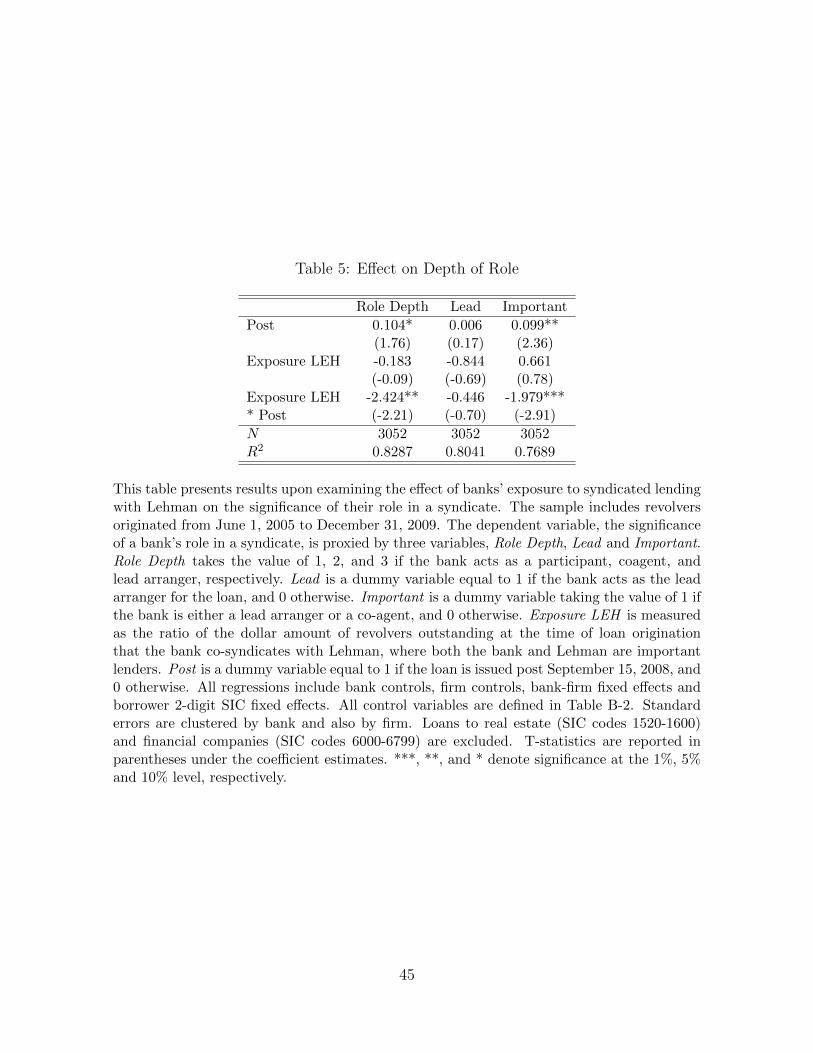
Table 5: Effect on Depth of Role

Role Depth Lead Important

Post 0.104* 0.006 0.099**(1.76) (0.17) (2.36)

Exposure LEH -0.183 -0.844 0.661(-0.09) (-0.69) (0.78)

Exposure LEH -2.424** -0.446 -1.979**** Post (-2.21) (-0.70) (-2.91)

N 3052 3052 3052R2 0.8287 0.8041 0.7689

This table presents results upon examining the effect of banks’ exposure to syndicated lendingwith Lehman on the significance of their role in a syndicate. The sample includes revolversoriginated from June 1, 2005 to December 31, 2009. The dependent variable, the significanceof a bank’s role in a syndicate, is proxied by three variables, Role Depth, Lead and Important.Role Depth takes the value of 1, 2, and 3 if the bank acts as a participant, coagent, andlead arranger, respectively. Lead is a dummy variable equal to 1 if the bank acts as the leadarranger for the loan, and 0 otherwise. Important is a dummy variable taking the value of 1 ifthe bank is either a lead arranger or a co-agent, and 0 otherwise. Exposure LEH is measuredas the ratio of the dollar amount of revolvers outstanding at the time of loan originationthat the bank co-syndicates with Lehman, where both the bank and Lehman are importantlenders. Post is a dummy variable equal to 1 if the loan is issued post September 15, 2008, and0 otherwise. All regressions include bank controls, firm controls, bank-firm fixed effects andborrower 2-digit SIC fixed effects. All control variables are defined in Table B-2. Standarderrors are clustered by bank and also by firm. Loans to real estate (SIC codes 1520-1600)and financial companies (SIC codes 6000-6799) are excluded. T-statistics are reported inparentheses under the coefficient estimates. ***, **, and * denote significance at the 1%, 5%and 10% level, respectively.

45

Table 6: Risky Borrowers

Importance level Important

IG (I) Non-IG (II) All (III) IG (IV) Non-IG (V) All (VI)

Post 0.015 0.204*** 0.16* 0.011 0.16*** 0.159***(0.13) (3.62) (1.86) (0.14) (3.63) (3.2)

Exposure LEH -1.697 1.312 -0.237 -0.054 1.211 0.926(-0.96) (0.24) (-0.10) (-0.06) (0.44) (0.93)

Exposure LEH * Post -0.733 -4.047** -2.964** -0.288 -3.112*** -2.81***(-1.21) (-2.34) (-1.99) (-0.73) (-2.76) (-3.17)

Investment Grade -0.065 -0.027(-0.74) (-0.59)

Investment Grade -0.071 -0.474* Exposure LEH (-0.06) (-0.56)Investment Grade -0.167 -0.168**** Post (-1.46) (-2.71)Investment Grade 1.857 2.312**** Exposure LEH * Post (1.22) (2.59)

N 1501 1551 3052 1501 1551 3052R2 0.8826 0.8505 0.8292 0.8462 0.7973 0.7704

This table presents results upon examining the effect of banks’ exposure to syndicated lendingwith Lehman on the significance of their role in a syndicate. The sample includes revolversoriginated from June 1, 2005 to December 31, 2009. Role Depth takes the value of 1, 2,and 3 if the bank acts as a participant, coagent, and lead arranger, respectively. Lead is adummy variable equal to 1 if the bank acts as the lead arranger for the loan, and 0 otherwise.Important is a dummy variable taking the value of 1 if the bank is either a lead arranger ora co-agent, and 0 otherwise. IG, Non-IG are the subsamples pertaining to investment gradeborrowers, and non-investment grade borrowers, respectively. All refers to the full sample.Exposure LEH is measured as the ratio of the dollar amount of revolvers outstanding at thetime of loan origination that the bank co-syndicates with Lehman, where both the bank andLehman are important lenders. Post is a dummy variable equal to 1 if the loan is issued postSeptember 15, 2008, and 0 otherwise. All regressions include bank controls, firm controls,bank-firm fixed effects and borrower 2-digit SIC fixed effects. All control variables are definedin Table B-2. Standard errors are clustered by bank and also by firm. Loans to real estate (SICcodes 1520-1600) and financial companies (SIC codes 6000-6799) are excluded. T-statisticsare reported in parentheses under the coefficient estimates. ***, **, and * denote significanceat the 1%, 5% and 10% level, respectively.

46

Table 7: Syndicate Diversification

SIC 1-digit SIC 2-digit FF 49 ind SIC 1-digit SIC 2-digit FF 49 ind

Post -0.018 0.009 0.005 -0.016 0.009 .006(-0.69) (0.36) (0.22) (-0.62) (0.38) (0.25)

Exposure LEH 0.44 -0.215 -0.215 0.503 -0.17 -0.167(0.63) (-1.44) (-1.02) (0.79) (-1.19) (-0.96)

Exposure LEH 0.75** 0.408 0.456* 0.6** 0.271 0.319* Post (2.49) (1.58) (1.82) (2.04) (1.15) (1.38)Lead 0.049* 0.029* 0.034*

(1.85) (1.73) (1.93)Lead*Post -0.041* -0.03* -0.033**

(-1.89) (-1.68) (-2)Lead*Exposure LEH -0.906** -0.662*** -0.729***

(-2.36) (-2.58) (2.86)Exposure LEH 0.9*** 0.722*** 0.76***Lead*Post (2.96) (2.58) (2.89)

N 2967 2967 2967 2967 2967 2967R2 0.8183 0.8567 0.8541 0.8199 0.8577 0.8552

This table reports coefficient estimates from regressions relating the distance between thebanks and their newly formed syndicate members to the banks’ existing exposure to syndicatedlending with Lehman via revolving lines of credit. The sample period is from June 1, 2005 toDecember 31, 2009. Exposure LEH is measured as the ratio of the dollar amount of revolversoutstanding at the time of loan origination that the bank co-syndicates with Lehman, whereboth the bank and Lehman are important lenders. Post is a dummy variable equal to 1 if theloan is issued post September 15, 2008, and 0 otherwise. SIC 1-digit/SIC 2-digit/FF 49 indrefers to specifications where the dependent variable, Distance, is measured based on 1-digit/2-digit borrower SIC codes/Fama and French (1994)’s 49 industry definition. All regressionsinclude bank controls, firm controls, bank-firm fixed effects and borrower 2-digit SIC fixedeffects. Control variables are defined in Table B-2. Standard errors are clustered by bankand also by firm. Loans to real estate (SIC codes 1520-1600) and financial companies (SICcodes 6000-6799) are excluded. T-statistics are reported in parentheses under the coefficientestimates. ***, **, and * denote significance at the 1%, 5% and 10% level, respectively.

47

Table 8: Syndicate Diversification: Important Lenders Versus Participants

Panel A: Syndicate Diversification: With Important Lenders Only

Sic 1-digit Sic 2-digit FF 49 ind Sic 1-digit Sic 2-digit FF 49 ind

Post -0.043* -0.016 -0.017 -0.043* -0.016 -0.016(-1.68) (-0.77) (-0.76) (-1.72) (-0.73) (-0.71)

Exposure LEH 0.498 -0.202 -0.184 0.593 -0.126 -1.103(0.59) (-1) (-0.64) (0.79) (-0.68) (-0.45)

Exposure LEH * Post 0.85** 0.423 0.456* 0.697** 0.3 0.321(2.27) (1.62) (1.72) (1.99) (1.31) (1.36)

Lead 0.093** 0.076*** 0.08***(2.3) (2.92) (2.83)

Lead*Post -0.039 -0.036 -0.04(-1.11) (-1.23) (-1.31)

Lead*Exposure LEH -1.579*** -1.3*** -1.369***(-2.84) (-3.52) (-3.64)

Lead*Exposure LEH 0.929** 0.796** 0.892***Post (2.22) (2.17) (2.32)

N 2850 2850 2850 2850 2850 2850R2 0.8458 0.8862 0.8791 0.8489 0.8879 0.8810

48

Panel B: Syndicate Diversification: With Participants OnlySic 1-digit Sic 2-digit FF 49 ind Sic 1-digit Sic 2-digit FF 49 ind

Post 0.032 0.055* 0.049 0.034 0.056* 0.05(1.03) (1.70) (1.58) (1.06) 1.67 (1.55)

Exposure LEH 0.406 -0.355* -0.318 0.42 -0.353* -0.319(0.65) (-1.68) (-1.33) (0.7) (-1.72) (-1.41)

Exposure LEH * Post 0.648** 0.423 0.463 0.522* 0.278 0.344(2.31) 1.38 (1.59) (1.82) 0.94 (1.2)

Lead 0.005 -0.026 -0.026(0.14) (-0.75) (-0.72)

Lead*Post -0.039 -0.023 -0.02(-1.25) (-0.59) (-0.5)

Lead*Exposure LEH -0.268 0.146 0.12(-0.51) (0.3) (0.24)

Lead*Exposure LEH 0.812 0.668 0.553*Post (1.49) (1.11) (0.92)N 2647 2647 2647 2647 2647 2647R2 0.7628 0.7896 0.79 0.7634 0.7903 0.7906

This table reports coefficient estimates from regressions relating the distance of newlyformed syndicates to the banks’ existing exposure to syndicated lending with Lehmanvia revolving lines of credit. The sample period is from June 1, 2005 to December31, 2009. In Panel A, Syndicate diversification is measured as the average distancebetween the lead arranger(s) and other important lenders (co-leads and co-agents) only.In Panel B, Syndicate diversification is measured as the average distance between thelead arranger(s) and syndicate participants only (co-leads and co-agents are excluded).Exposure LEH is measured as the ratio of the dollar amount of revolvers outstandingat the time of loan origination that the bank co-syndicates with Lehman, where boththe bank and Lehman are important lenders. Post is a dummy variable equal to 1 if theloan is issued post September 15, 2008, and 0 otherwise. SIC 1-digit/SIC 2-digit/FF 49ind refers to specifications where the dependent variable, distance, is measured basedon 1-digit/2-digit borrower SIC codes/Fama and French (1994)’s 49 industry definition.All regressions include bank controls, firm controls, bank-firm fixed effects and borrower2-digit SIC fixed effects. Control variables are defined in Table B-2. Standard errorsare clustered by bank and also by firm. Loans to real estate (SIC codes 1520-1600) andfinancial companies (SIC codes 6000-6799) are excluded. T-statistics are reported inparentheses under the coefficient estimates. ***, **, and * denote significance at the1%, 5% and 10% level, respectively.

49

Table 9: Robustness Tests

Panel A: Logit Regressions

Role (I) Lead (II) Important (III)

Post 1.268*** 1.606* 1.805***(10.78) (4.031) (12)

Exposure LEH 6.186 -30.236 15.68(0.74) (2.18) 2.39

Exposure LEH -22.47*** -39.168*** -32.356**** Post 23.61 (10.86) (27.28)

N 3052 3052 3052PseudoR2 0.8689 0.9012 0.8787

Panel B: Excluding Banks with Zero Exposure

Role Lead Important Maturity Sic Sic FFDepth 1-digit 2-digit 49 ind

Post 0.106 0.004 0.101** -1.677 -0.002 0.023 0.021( 1.47) (0.12) (2.17) (-0.51) (-0.09) (1.01) (1.02)

Exposure LEH -0.132 -0.817 0.684 68.38 0.523 -0.142 -0.136-0.07 (-0.67) ( 0.79) (1.34) (0.8) (-0.96) (-0.72)

Exposure LEH -2.448** -0.477 -1.972*** -55.787** 0.448 0.118 0.146* Post (-2.02) 0.71 (-2.66) (-2.20) ( 1.62) (0.56) (0.77)Lead 0.053** 0.033* 0.038**

(2.01) (1.92) (2.14)Lead*post -0.048** -0.037** -0.041***

(-2.18) (-2.17) (-2.63)Lead* Exposure LEH -0.959** -0.69*** -0.765***

(-2.46) (2.7) (-2.99)Exposure LEH 0.972*** 0.798*** 0.845****Post * Lead (3.19) (2.97) (3.40)

N 2907 2907 2907 2895 2849 2849 2849R2 0.8221 0.7992 0.7604 0.5832 0.7759 0.8259 0.8212

50

Panel C: Placebo Tests

Role Lead Important Maturity Sic Sic FFDepth 1-digit 2-digit 49 ind

Post -0.057 -0.028 -0.029 -4.144** -0.026 -0.013 -0.001(-1.36) (-1.58) (-0.86) (-2.04) (-0.86) (-0.48) (-0.04)

Exposure LEH 1.127 -0.278 1.405*** 37.575 0.791 0.307 0.195(1.63) (-0.61) (2.98) (1.22) (1.05) (0.53) (0.29)

Exposure LEH 0.643 0.261 0.382 8.198 0.989* 0.835* 0.611* Post (1.09) (0.79) (0.89) (0.31) (1.94) (1.86) (1.4)Lead 0.004 -0.014 -0.01

(0.14) (-0.65) (-0.46)Lead * Post 0.086 * 0.077** 0.06*

(1.92) (2.11) (1.7)Exposure LEH -0.225 0.042 -0.028*Lead (-0.65) (0.14) (-0.09)Exposure LEH -1.137 -1.026* -0.763* Lead * Post (-1.63) (-1.86) (-1.37)

N 6359 6359 6359 6312 6359 6359 6459R2 0.8361 0.8250 0.4959 0.8340 0.8632 0.8586

This table reports results from robustness tests. Panel A: Presents results from esti-mating (6) using conditional ordinal logit regression for Lead and Important Column(I), and from conditional logit regressions for Role Depth(columns (II) and (III)); Waldstatistics are in parentheses under coefficient estimates. Panels B and C report ro-bustness for the main tests regarding the importance of syndicate roles and syndicatediversification. Role Depth takes the value of 1, 2, and 3 if the bank acts as a partici-pant, coagent, and lead arranger, respectively. Lead is a dummy variable equal to 1 ifthe bank acts as the lead arranger for the loan, and 0 otherwise. Important is a dummyvariable taking the value of 1 if the bank is either a lead arranger or a co-agent, and 0otherwise. SIC 1-digit/SIC 2-digit/FF 49 ind refers to specifications where the depen-dent variable, distance, is measured based on 1-digit/2-digit borrower SIC codes/Famaand French (1994)’s 49 industry definition. Panel B: Excluding zero-exposure banksfrom the sample; Panel C: the placebo period from March 1, 2004 to September 15,2008, with the placebo event date being June 15, 2007. All regressions include bankcontrols, firm controls, bank-firm fixed effects and borrower 2-digit SIC fixed effects.Exposure LEH is the fraction of the dollar amount of outstanding revolvers that thebank co-syndicates with Lehman, where both the bank and Lehman are importantlenders. Control variables are defined in Table B-2. Standard errors are clustered bybank and also by firm.

51

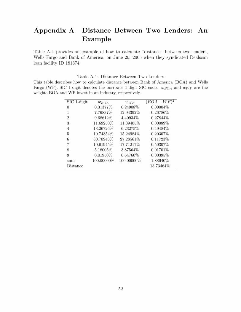
Appendix A Distance Between Two Lenders: An

Example

Table A-1 provides an example of how to calculate “distance” between two lenders,Wells Fargo and Bank of America, on June 20, 2005 when they syndicated Dealscanloan facility ID 181374.

Table A-1: Distance Between Two LendersThis table describes how to calculate distance between Bank of America (BOA) and WellsFargo (WF). SIC 1-digit denotes the borrower 1-digit SIC code. wBOA and wWF are theweights BOA and WF invest in an industry, respectively.

SIC 1-digit wBOA wWF (BOA−WF )2

0 0.31377% 0.24908% 0.00004%1 7.76837% 12.94392% 0.26786%2 9.68612% 4.40934% 0.27844%3 11.69250% 11.39405% 0.00089%4 13.26726% 6.23275% 0.49484%5 10.74354% 15.24984% 0.20307%6 30.70943% 27.28561% 0.11723%7 10.61945% 17.71217% 0.50307%8 5.18005% 3.87564% 0.01701%9 0.01950% 0.64760% 0.00395%sum 100.00000% 100.00000% 1.88640%Distance 13.73464%

52

Appendix B Additional Tables

Table B-2: Definition of Variables

Variable Name Definition

Banks (Source:Call Reports)

Assets RCFD2170ROA RIAD4340/RCFD2170Core Deposits (RCON2702+RCON2215)/RCFD2170Subordinated Debt RCFD3200/RCFD2170Capital RCFD3210/RCFD2170Loan Loss (RIAD4635-RIAD4605)/RCFD2170

Firms (Source: Compustat)

Sales SaleqLeverage (Dlttq+dlcq)/atqInterest Coverage Oibdpq/xintqNet Working Capital (atq-lctq)/(Dlttq+dlcq)Tangibles (ppentq+invtq)/atqFirm Age Year of facility first year in Compustat

Loans (Source: Dealscan)

Al-in-drawn Spread AllInDrawnAmount FacilityamtMaturity MaturityInvestment Grade Market Segment

All income variables from Call Reports (RIAD4340, RIAD4635, and RIAD4605) areadjusted to be quarterly values from the reported year-to-date figures. Definition ofitem abbreviations are as follows. RCFD2170 is total assets; RIAD4340 is net income(loss); RCON2702 is the amount of deposits accounts of $100,000 or less; RCON2215is the amount of transaction accounts; RCFD3200 is the amount of subordinated notesand debentures; RCFD3210 is the total amount of equity capital; RIAD4635 is theamount of charge-offs on allowance for loan and lease losses. RIAD4605 is the amountof recoveries on allowance for loan and lease losses; Dlttq/dlcq is total value of longterm debt/debt in current liabilities; Oibdpq is Operating Income Before Depreciation;xintq is the amount of interest and related expense; lctq is the amount of currentliabilities; ppentq is the value of property, plant, and equipment; invtq is the totalvalue of inventories.

53

Table B-3: Effect on Depth of Role and Syndicate Diversification: Term Loans

Role Lead Important SIC 1 SIC 2 FF 49Depth (I) (II) (III) -digit (IV) -digit (V) ind (VI)

Post -0.12 -0.087 -0.034 -0.047 -0.04 -0.042(-0.38) (-0.54) (-0.16) (-1.01) (-0.81) (-0.82)

Exposure LEH 4.346 3.031 1.315 -1.354 -0.988 -1.043(1.3) (0.79) (0.39) (-0.99) (-0.74) (-0.83)

Exposure LEH 2.032 2.407 -0.375 1.203 1.043 1.145* Post (0.45) (1.2) (-0.12) (1.39) (1.1) (1.21)Lead 0.067 0.059 0.065

(1.05) (0.83) (0.92)Lead * Post -0.073 -0.056 -0.081

(-1.18) (-0.8) (-1.05)Lead*Exposure LEH -0.915 -0.803 -0.922

(-0.95) (-0.74) (-0.83)Exposure LEH 0.63 0.397 0.680Lead * Post 0.71 (0.38) (0.62)

N 603 603 603 573 573 573R2 0.7568 0.7231 0.6933 0.8036 0.8325 0.8301

This table presents results upon examining the effect of banks’ exposure to syndicated re-volvers with Lehman on the significance of their role in a syndicate (columns (I)-(III)), andsyndicate diversification (columns (IV)-(VI)). The sample consists of term loans originatedfrom June 1, 2005 to December 31, 2009. The significance of a bank in a syndicate, is proxiedby three variables, Role Depth, Lead, and Important. Role Depth takes the value of 1, 2,and 3 if the bank acts as a participant, coagent, and lead arranger, respectively. Lead is adummy variable equal to 1 if the bank acts as the lead arranger of the loan syndicate, and 0otherwise. Important is a dummy variable equal to 1 if the bank is either a lead arranger ora co-agent of the loan syndicate, and 0 otherwise. SIC 1-digit/SIC 2-digit/FF 49 ind refersto specifications where the dependent variable, distance, is measured based on 1-digit/2-digitborrower SIC codes/Fama and French’s 49 industry definition. Exposure LEH is the ratioof the dollar amount of revolvers outstanding at the time of loan origination that the bankco-syndicate with Lehman, where both the bank and Lehman are important lenders. Post isa dummy variable equal to 1 if the loan is issued post September 15, 2008, and 0 otherwise.All regressions include bank controls, firm controls, bank-firm fixed effects and borrower 2-digit SIC fixed effects. Control variables related to lenders (Log assets, ROA, Core Deposits,Subordinated Debt, Capital and Loan Loss) and borrowers (Log Sales, Leverage, InterestCoverage, Net Working Capital, Tangibles, Firm Age, Investment Grade) are defined in Ta-ble B-2. Standard errors are clustered by bank and also by firm. Loans to real estate (SICcodes 1520-1600) and financial companies (SIC codes 6000-6799) are excluded. T-statisticsare reported in parentheses under the coefficient estimates. ***, **, and * denote significanceat the 1%, 5% and 10% level, respectively.

54