Risk-sensitive Inverse Reinforcement Learningvia Coherent Risk Models

Anirudha Majumdar†, Sumeet Singh†, Ajay Mandlekar∗, and Marco Pavone††Department of Aeronautics and Astronautics, ∗Electrical Engineering

Stanford University, Stanford, CA 94305Email: anirudha,ssingh19,amandlek,pavone@stanford.edu

Abstract—The literature on Inverse Reinforcement Learning(IRL) typically assumes that humans take actions in order tominimize the expected value of a cost function, i.e., that humansare risk neutral. Yet, in practice, humans are often far frombeing risk neutral. To fill this gap, the objective of this paper isto devise a framework for risk-sensitive IRL in order to explicitlyaccount for an expert’s risk sensitivity. To this end, we proposea flexible class of models based on coherent risk metrics, whichallow us to capture an entire spectrum of risk preferences fromrisk-neutral to worst-case. We propose efficient algorithms basedon Linear Programming for inferring an expert’s underlying riskmetric and cost function for a rich class of static and dynamicdecision-making settings. The resulting approach is demonstratedon a simulated driving game with ten human participants. Ourmethod is able to infer and mimic a wide range of qualitativelydifferent driving styles from highly risk-averse to risk-neutralin a data-efficient manner. Moreover, comparisons of the Risk-Sensitive (RS) IRL approach with a risk-neutral model showthat the RS-IRL framework more accurately captures observedparticipant behavior both qualitatively and quantitatively.

I. INTRODUCTION

Imagine a world where robots and humans coexist and workseamlessly together. In order to realize this vision, robots mustbe able to (1) accurately predict the actions of humans intheir environment, (2) quickly learn the preferences of humanagents in their proximity and act accordingly, and (3) learnhow to accomplish new tasks from human demonstrations.Inverse Reinforcement Learning (IRL) [41, 32, 2, 29, 38, 50,16] is a powerful and flexible framework for tackling thesechallenges and has been previously used for tasks such asmodeling and mimicking human driver behavior [1, 28, 43],pedestrian trajectory prediction [51, 31], and legged robotlocomotion [52, 27, 35]. The underlying assumption behindIRL is that humans act optimally with respect to an (unknown)cost function. The goal of IRL is then to infer this cost functionfrom observed actions of the human. By learning the human’sunderlying preferences (in contrast to, e.g., directly learning apolicy for a given task), IRL allows one to generalize one’spredictions to novel scenarios and environments.

The prevalent modeling assumption made by existing IRLtechniques is that humans take actions in order to minimizethe expected value of a cost function. This modeling as-sumption corresponds to the expected utility/cost (EU) theoryin economics [47]. Despite the historical prominence of EUtheory in modeling human behavior, a large body of literaturefrom the theory of human decision making strongly suggeststhat humans behave in a manner that is inconsistent withan EU model. An elegant illustration of this is the Ellsbergparadox [15]. Imagine an urn (Urn 1) containing 50 red and50 black balls. Urn 2 also contains 100 red and black balls,but the relative composition of colors is unknown. Suppose

(a) Visualization of screen seen by human. (b) Joystick setup.

Fig. 1: The simulated driving game considered in this paper. The humancontrols the follower car using a joystick and must follow the leader (an“erratic driver”) as closely as possible without colliding. We observed a widerange of behaviors from participants reflecting varying attitudes towards risk.

that there is a payoff of $10 if a red ball is drawn (and nopayoff for black). In human experiments, subjects display anoverwhelming preference towards having a ball drawn fromUrn 1. However, now suppose the subject is told that a blackball has $10 payoff (and no payoff for red). Humans still preferto draw from Urn 1. But, this is a paradox since choosing todraw from Urn 1 in the first case (payoff for red) indicatesthat the proportion of red in Urn 1 is higher than in Urn 2,while choosing Urn 1 in the second case (payoff for black)indicates a lower proportion of red in Urn 1 than in Urn 2.

Intuitively, there are two main limitations of EU theory:(1) the standard model assumes that humans are risk neutralwith respect to their utility function, and (2) it assumesthat humans make no distinction between scenarios in whichthe probabilities of outcomes are known (e.g., Urn 1 inthe Ellsberg paradox) and ones in which the outcomes areunknown (e.g., Urn 2). The known and unknown probabilityscenarios are referred to as risky and ambiguous respectivelyin the decision theory literature. While EU theory does allowsome consideration of risk, e.g., via concave utility functions,experimental results demonstrate that it is not a good modelfor human behavior in risky scenarios [26]. This has promptedwork on various non-EU theories (see e.g., [5, 15, 26, 9]).Further, one way to interpret the Ellsberg paradox is thathumans are not only risk averse, but are also ambiguityaverse – an observation that has sparked an alternative set ofliterature in decision theory on “ambiguity-averse” modeling;see, e.g., the recent review [18]. The assumptions made by EUtheory thus represent significant restrictions from a modelingperspective in an IRL context since a human expert is likelyto be risk and ambiguity averse, especially in safety criticalapplications such as driving where outcomes are inherentlyambiguous and can possibly incur very high cost.

The key insight of this paper is to address these challengesby modeling humans as evaluating costs according to an(unknown) risk metric. A risk metric is a function that mapsan uncertain cost to a real number (the expected value is thusa particular risk metric and corresponds to risk neutrality). Inparticular, we will consider the class of coherent risk metrics(CRMs) [7, 44, 42]. These metrics were introduced in theoperations research literature and have played an influentialrole within the modern theory of risk in finance [40, 4, 3, 39].This theory has also recently been adopted for risk-sensitive(RS) Model Predictive Control and decision making [12, 13],and autonomous exploration [8].

Coherent risk metrics enjoy a number of advantages overEU theory in the context of IRL. First, they capture an entirespectrum of risk assessments from risk-neutral to worst-caseand thus offer a significant degree of modeling flexibility (notethat EU theory is a special case of a coherent risk model). Sec-ond, they capture risk sensitivity in an axiomatically justifiedmanner; they formally capture a number of intuitive notionsthat one would expect any risk metric to satisfy (ref. SectionII-B). Third, a representation theorem for CRMs (Section II-B)implies that they can be interpreted as computing the expectedvalue of a cost function in a worst-case sense over a setof probability distributions (referred to as the risk envelope).Thus, CRMs capture both risk and ambiguity aversion withinthe same modeling framework since the risk envelope canbe interpreted as capturing uncertainty about the underlyingprobability distribution that generates outcomes in the world.Finally, they are tractable from a computational perspective;the representation theorem allows us to solve both the inverseand forward problems in a computationally tractable mannerfor a rich class of static and dynamic decision-making settings.

Statement of contributions: To our knowledge, the resultsin this paper constitute the first attempt to explicitly take intoaccount risk sensitivity in the context of IRL under generalaxiomatically justified risk models that jointly capture risk andambiguity. To this end, this paper makes three primary contri-butions. First, we propose a flexible modeling framework forcapturing risk sensitivity in experts by assuming that the expertacts according to a CRM. This framework allows us to capturean entire spectrum of risk assessments from risk-neutral toworst-case. Second, we develop efficient algorithms based onLinear Programming (LP) for inferring an expert’s underlyingrisk metric for a broad range of static (Section III) anddynamic (Section IV) decision-making settings. We considercases where the expert’s underlying risk metric is unknownbut the cost function is known, and also the more generalcase where both are unknown. Third, we demonstrate ourapproach on a simulated driving game (visualized in Figure 1)and present results on ten human participants (Section V). Weshow that our approach is able to infer and mimic qualitativelydifferent driving styles ranging from highly risk-averse torisk-neutral using only a minute of training data from eachparticipant. We also compare the predictions made by ourrisk-sensitive IRL (RS-IRL) approach with one that modelsthe expert using EU theory and demonstrate that the RS-IRL framework more accurately captures observed participantbehavior both qualitatively and quantitatively.

Related Work: Restricted versions of the problems consid-ered here have been studied before. In particular, there is alarge body of work on RS decision making. For instance,

in [24] the authors leverage the exponential (or entropic)risk. This has historically been a very popular technique forparameterizing risk-attitudes in decision theory but suffersfrom the usual drawbacks of the EU framework as eluci-dated in [37]. Other RS Markov Decision Process (MDP)formulations include Markowitz-inspired mean-variance [17]and percentile-based risk measures (e.g., Conditional value-at-risk (CVaR) [10]). This has driven research in the designof learning-based solution algorithms, i.e., RS reinforcementlearning [30, 46, 36, 45]. Ambiguity in MDPs is also wellstudied via the robust MDP framework, see e.g., [33, 49], aswell as [34, 13] where the duality between risk and ambiguityas a result of CRMs is exploited. The key difference betweenthis literature and the present work is that we consider theinverse reinforcement learning problem.

Results in the RS-IRL setting are more limited and havelargely been pursued in the neuroeconomics literature [21].For example, [25] performed Functional Magnetic ResonanceImaging (FMRI) studies of humans making decisions in riskyand ambiguous settings and modeled risk and ambiguity aver-sion using parametric utility and weighted probability models.In a similar vein, [45] models risk aversion using utility basedshortfalls and presents FMRI studies on humans performinga sequential investment task. While this literature may beinterpreted in the context of IRL, the models used to predictrisk and ambiguity aversion are quite limited. For example,shortfall is fixed as the risk metric in [45] while estimatingparameters in a utility model. In contrast, the class of riskmetrics we consider are significantly more flexible.

II. PROBLEM FORMULATION

A. DynamicsConsider the following discrete-time dynamical system:

xk+1 = f(xk, uk, wk), (1)

where k is the time index, xk ∈ Rn is the state, uk ∈ Rmis the control input, and wk ∈ W is the disturbance. Thecontrol input is assumed to be bounded component-wise:uk ∈ U := u : u− ≤ u ≤ u+. We take W to bea finite set w[1], . . . , w[L] with probability mass function(pmf) p := [p(1), p(2), . . . , p(L)], where

∑Li=1 p(i) = 1

and p(i) > 0,∀i ∈ 1, . . . , L. The time-sampling of thedisturbance wk will be discussed in Section IV. We assumethat we are given demonstrations from an expert in the formof sequences of state-control pairs (x∗k, u∗k)k and that theexpert has knowledge of the underlying dynamics (1) but doesnot necessarily have access to the disturbance set pmf p.

B. Model of the ExpertWe model the expert as a risk-aware decision-making agent

acting according to a coherent risk metric (defined formallybelow). We refer to such a model as a coherent risk model.

We assume that the expert has a cost function C(xk, uk) thatcaptures his/her preferences about outcomes. Let Z denote thecumulative cost accrued by the agent over a horizon N :

Z :=

N∑k=0

C(xk, uk). (2)

Note that since the process xk is stochastic, Z is a randomvariable adapted to the sequence xk. A risk metric is a

function ρ(Z) that maps this uncertain cost to a real number.We will assume that the expert is assessing risks according toa coherent risk metric, defined as follows.Definition 1 (Coherent Risk Metrics). Let (Ω,F ,P) be aprobability space and let Z be the space of random variableson Ω. A coherent risk metric (CRM) is a mapping ρ : Z → Rthat obeys the following four axioms. For all Z,Z ′ ∈ Z:

A1. Monotonicity: Z ≤ Z ′ ⇒ ρ(Z) ≤ ρ(Z ′).A2. Translation invariance: ∀a ∈ R, ρ(Z+a) = ρ(Z)+a.A3. Positive homogeneity: ∀λ ≥ 0, ρ(λZ) = λρ(Z).A4. Subadditivity: ρ(Z + Z ′) ≤ ρ(Z) + ρ(Z ′).These axioms were originally proposed in [7] to ensure the

“rationality” of risk assessments. For example, A1 states thatif a random cost Z is less than or equal to a random costZ ′ regardless of the disturbance realizations, then Z must beconsidered less risky (one may think of the different randomcosts arising from different control policies). A4 reflects theintuition that a risk-averse agent should prefer to diversify.We refer the reader to [7] for a thorough justification of theseaxioms. An important characterization of CRMs is providedby the following representation theorem.Theorem 1 (Representation Theorem for Coherent Risk Met-rics [7]). Let (Ω,F ,P) be a probability space, where Ω isa finite set with cardinality |Ω|, F is the σ−algebra oversubsets (i.e., F = 2Ω), probabilities are assigned according toP = (p(1), p(2), . . . , p(|Ω|)), and Z is the space of randomvariables on Ω. Denote by C the set of valid probabilitydensities:

C :=

ζ ∈ R|Ω| ||Ω|∑i=1

p(i)ζ(i) = 1, ζ ≥ 0

. (3)

Define qζ ∈ R|Ω| where qζ(i) = p(i)ζ(i), i = 1, . . . , |Ω|. Arisk metric ρ : Z → R with respect to the space (Ω,F ,P) isa CRM if and only if there exists a compact convex set B ⊂ Csuch that for any Z ∈ Z:

ρ(Z) = maxζ∈B

Eqζ [Z] = maxζ∈B

|Ω|∑i=1

p(i)ζ(i)Z(i). (4)

This theorem is important for two reasons. Conceptually, itgives us an interpretation of CRMs as computing the worst-case expectation of the cost function over a set of densitiesB (referred to as the risk envelope). Coherent risks thusallow us to consider risk and ambiguity (ref. Section I) ina unified framework since one may interpret an agent actingaccording to a coherent risk model as being uncertain aboutthe underlying probability density. Second, it provides us withan algorithmic handle over CRMs and will form the basis ofour approach to measuring experts’ risk preferences.

In this work, we will take the risk envelope B to be apolytope. We refer to such risk metrics as polytopic riskmetrics, which were also considered in [14]. By absorbingthe density ζ into the pmf p, we can represent (without lossof generality) a polytopic risk metric as:

ρ(Z) = maxp∈P

Ep[Z], (5)

where P is a polytopic subset of the probability simplex:

P =p ∈ ∆|Ω| | Aineqp ≤ bineq

, (6)

where ∆|Ω| := p ∈ R|Ω| |∑|Ω|i=1 p(i) = 1, p ≥ 0. Polytopic

risk metrics constitute a rich class of risk metrics, encom-passing a spectrum ranging from risk neutrality (P = p)to worst-case assessments (P = ∆|Ω|). Examples includeCVaR, mean absolute semi-deviation, spectral risk measures,optimized certainty equivalent, and the distributionally robustrisk [12]. We further note that the ambiguity interpretationof CRMs is reminiscent of Gilboa & Schmeidler’s MinmaxEU model for ambiguity-aversion [19] which was shown tooutperform various competing models in [22] for single-stagedecision problems, albeit with more restrictions on the set B.

Goal: Given demonstrations from the expert in the formof state-control trajectories, our goal will be to conservativelyapproximate the expert’s risk preferences by finding an outerapproximation of the risk envelope P .

III. RISK-SENSITIVE IRL: SINGLE DECISION PERIOD

In this section we consider the single step decision problem,i.e., N = 0 in equation (2). Thus, the probability space(Ω,F ,P) is simply (W, 2W , p).

A. Known Cost FunctionWe first consider the static decision-making setting where

the expert’s cost function is known but the risk metric isunknown. A coherent risk model then implies that the expertis solving the following optimization problem at state x inorder to compute an optimal action:

τ∗ := minu∈U

ρ(C(x, u)) = minu∈U

maxp∈P

Ep[C(x, u)] (7)

:= minu∈U

maxp∈P

g(x, u)T p, (8)

where ρ(·) is a CRM with respect to the space (W, 2W , p)(i.e., P ⊆ ∆L). In the last equation, g(x, u)(j) is the costwhen the disturbance w[j] ∈ W is realized. Since the innermaximization problem is linear in p, the optimal value isachieved at a vertex of the polytope P . Denoting the setof vertices of P as vert(P ) = vii∈1,...,NV , we can thusrewrite problem (7) above as follows:

minu∈U,τ

τ (9)

s.t. τ ≥ g(x, u)T vi, i ∈ 1, . . . , NV

If the cost function C(·, ·) is convex in the control inputu, the resulting optimization problem is convex. Given adataset D = (x∗,d, u∗,d)Dd=1 of state-control pairs of theexpert taking action u∗,d at state x∗,d, our goal is to deducea conservative approximation (i.e., an outer approximation)Po of P from the given data. The key idea of our technicalapproach is to examine the Karush-Kuhn-Tucker (KKT) con-ditions for Problem (9). The use of KKT conditions for InverseOptimal Control is a technique also adopted in [16]. The KKTconditions are necessary for optimality in general and are alsosufficient in the case of convex problems. We can thus usethe KKT conditions along with the dataset D to constrain theconstraints of Problem (9). In other words, the KKT conditionswill allow us to constrain where the vertices of P must lie inorder to be consistent with the fact that the state-control pairsrepresent optimal solutions to Problem (9). Importantly, wewill not assume access to the number of vertices NV of P .

Let (x∗, u∗) be an optimal state-control pair and let J +

and J− denote the sets of components of the control input u∗

that are saturated above and below respectively (i.e., u(j) =u+(j),∀j ∈ J + and u(j) = u−(j),∀j ∈ J−).Theorem 2. Consider the following optimization problem:

maxv∈∆L

σ+,σ−≥0

g(x∗, u∗)T v (10)

s.t. 0 = ∇u(j)g(x, u)T v∣∣∣x∗,u∗

+ σ+(j),∀j ∈ J+

0 = ∇u(j)g(x, u)T v∣∣∣x∗,u∗

− σ−(j),∀j ∈ J−.

0 = ∇u(j)g(x, u)T v∣∣∣x∗,u∗

, ∀j /∈ J+, j /∈ J−.

Denote the optimal value of this problem by τ ′ and define thehalfspace:

H(x∗,u∗) := v ∈ RL | τ ′ ≥ g(x∗, u∗)T v. (11)

Then, the risk envelope P satisfies P ⊂ (H(x∗,u∗) ∩∆L).

Proof: The KKT conditions for Problem (9) are:

1 =

NV∑i=1

λi, (12)

0 = λi[g(x∗, u∗)T vi − τ ], i = 1, . . . , NV , (13)For j = 1, . . . ,m :

0 = σ+(j)− σ−(j) +

NV∑i=1

λi ∇u(j)g(x, u)T vi

∣∣∣x∗,u∗

, (14)

0 = σ+(j)[u∗(j)− u+(j)], 0 = σ−(j)[u−(j)− u∗(j)], (15)

where λi, σ+(j), σ−(j) ≥ 0 are multipliers. Now, supposethere are multiple optimal vertices vii∈I for Problem (9)in the sense that τ∗ = g(x∗, u∗)T vi, ∀i ∈ I. Defining v :=∑i∈I λivi, we see that v satisfies:

0 = ∇u(j)g(x∗, u∗(j))T v + σ+(j)− σ−(j), j = 1, . . . ,m, (16)

and τ∗ = g(x∗, u∗)T v since∑i∈I λi = 1. Now, since v

satisfies the constraints of Problem (10) (which are implied bythe KKT conditions), it follows that τ ′ ≥ τ∗. From problem(9), we see that τ ′ ≥ τ∗ ≥ g(x∗, u∗)T vi, ∀vi ∈ vert(P) andthus P ⊂ (H(x∗,u∗) ∩∆L).

Problem (10) is a Linear Program (LP) and can thus besolved efficiently. For each demonstration (x∗,d, u∗,d) ∈ D,Theorem 2 provides a halfspace constraint on the risk envelopeP . By aggregating these constraints, we obtain a polytopicouter approximation Po of P . This is summarized in Algo-rithm 1. Note that Algorithm 1 operates sequentially throughthe data D and is thus directly applicable in online settings.

Algorithm 1 Outer Approximate Risk Envelope

1: Initialize Po = ∆L

2: for d = 1, . . . , D do3: Solve Linear Program (10) with (x∗,d, u∗,d) to obtain a

hyperplane H(x∗,d,u∗,d)

4: Update Po ← Po ∩H(x∗,d,u∗,d)

5: end for6: Return Po

As we collect more half-space constraints in Algorithm 1,the constraint v ∈ ∆L in Problem (10) above can be replacedby v ∈ Po, where Po is the current outer approximation of therisk envelope. It is easily verified that the results of Theorem 2

still hold. This allows us to obtain a tighter (i.e., lower) upperbound τ ′ for τ∗, thus resulting in tighter halfspace constraints.

Once we have recovered an outer approximation Po of P ,we can solve the “forward” problem (i.e., compute actions ata given state x) by solving the optimization problem (7) withPo as the risk envelope.

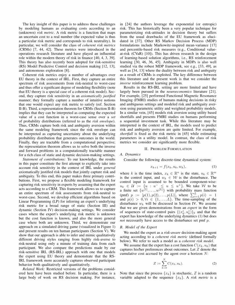
1) Example: Linear-Quadratic System: As a simple illus-trative example to gain intuition for the convergence prop-erties of Algorithm 1, consider a linear dynamical systemwith multiplicative uncertainty of the form f(xk, uk, wk) =A(wk)xk + B(wk)uk. We consider the one-step decision-making process with a quadratic cost on state and action:Z := uT0 Ru0 + xT1 Qx1, where x1 = A(w0)x0 + B(w0)u0.Here, R 0 and Q 0. We consider a 10-dimensional statespace with a 5-dimensional control input space. The number ofrealizations is taken to be L = 3 for ease of visualization. TheL different A(wk) and B(wk) matrices corresponding to eachrealization are generated randomly by independently samplingelements of the matrices from the standard normal distributionN (0, 1). The cost matrix Q is a randomly generated psd matrixand R is the identity. States x∗ are drawn from N (0, 1).

Figure 2 shows the outer approximations of the risk en-velope obtained using Algorithm 1. We observe rapid con-vergence (approximately 20 sampled states x∗) of the outerapproximations Po (red) to the true risk envelope P (green).

(a) 5 data points (b) 20 data points

Fig. 2: Rapid convergence of the outer approximation of the risk envelope.

B. Unknown Cost FunctionNow we consider the more general case where both the

expert’s cost function and risk metric are unknown. We param-eterize our cost function as a linear combination of featuresin (x, u). Then, the expected value of the cost function w.r.t.p ∈ ∆L can be written as g(x, u)T p, where:

g(x, u)(j) =

H∑h=1

c(h)φj,h(x, u), j = 1, . . . , L, (17)

with nonnegative weights c ∈ RH≥0. Since the solution ofproblem (7) solved by the expert is invariant to positivescalings of the cost function due to the positive homogeneityproperty of coherent risks (ref. Definition 1), we can assumewithout loss of generality that the feature weights sum to 1.

With this cost structure, we see that the KKT conditionsderived in Section III-A involve products of the feature weightsc and the vertices vi of P . Similarly, an analogous versionof optimization problem (10) can be used to bound theoptimal value. This problem again contains products of theunknown feature weights c and the probability vertex v. Thekey idea here is to introduce new decision variables z that

replace each product v(j)c(h) by a new variable zjh whichallows us to re-write problem (10) as an LP in (z, σ+, σ−),with the addition of the following two simple constraints:0 ≤ zjh ≤ 1,∀j, h,

∑j,h zjh = 1. In a manner analogous

to Theorem 2, this optimization problem allows us to obtainbounding hyperplanes in the space of product variables zwhich can then be aggregated as in Algorithm 1. Denoting thispolytope as Pz , we can then proceed to solve the “forward”problem (i.e., computing actions at a given state x) by solvingthe following optimization problem:

minu∈U

maxz∈Pz

∑j,h

zjhφj,h(x, u). (18)

This problem can be solved by enumerating the vertices of thepolytope Pz in a manner similar to problem (9).Remark 1. While the above procedure operates in the space ofproduct variables z and does not require explicitly recoveringthe cost function and risk envelope separately, it may neverthe-less be useful to do so in order to obtain additional insightsinto the expert’s decision-making process and generalize tonovel scenarios. We have explored an approach for doing this,but will defer the results to an extended version of this workdue to space limitations.

IV. RISK-SENSITIVE IRL: MULTI-STEP CASE

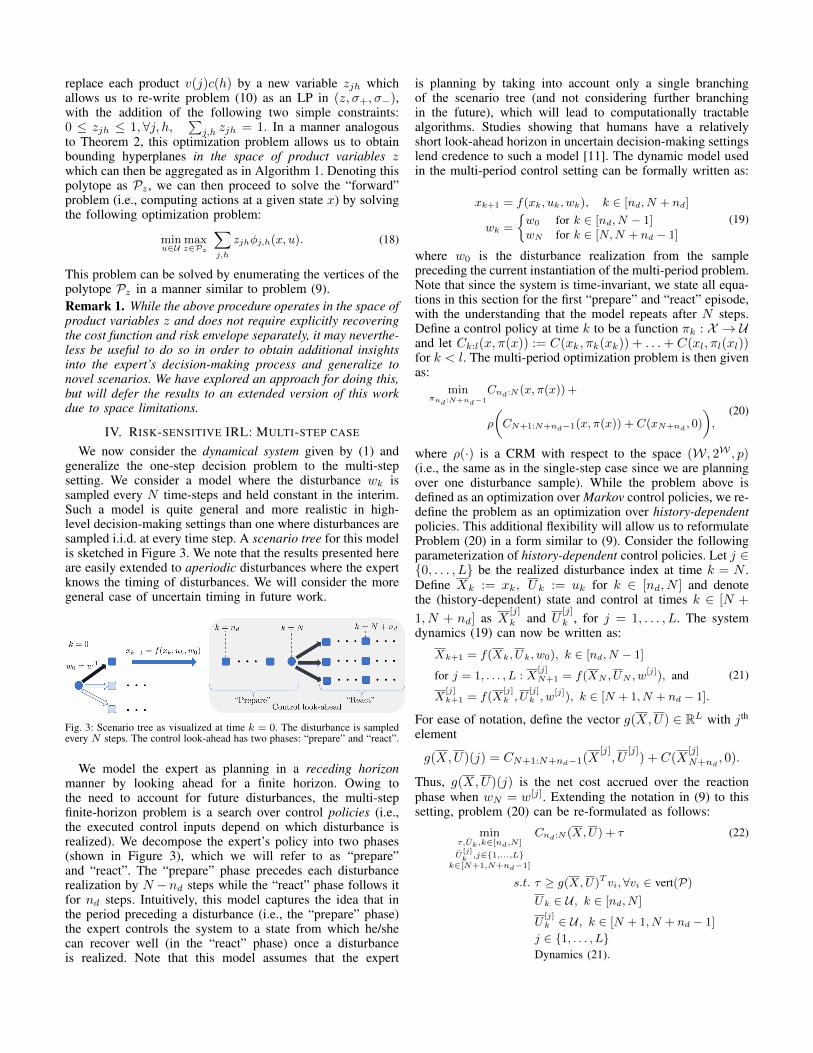
We now consider the dynamical system given by (1) andgeneralize the one-step decision problem to the multi-stepsetting. We consider a model where the disturbance wk issampled every N time-steps and held constant in the interim.Such a model is quite general and more realistic in high-level decision-making settings than one where disturbances aresampled i.i.d. at every time step. A scenario tree for this modelis sketched in Figure 3. We note that the results presented hereare easily extended to aperiodic disturbances where the expertknows the timing of disturbances. We will consider the moregeneral case of uncertain timing in future work.

Fig. 3: Scenario tree as visualized at time k = 0. The disturbance is sampledevery N steps. The control look-ahead has two phases: “prepare” and “react”.

We model the expert as planning in a receding horizonmanner by looking ahead for a finite horizon. Owing tothe need to account for future disturbances, the multi-stepfinite-horizon problem is a search over control policies (i.e.,the executed control inputs depend on which disturbance isrealized). We decompose the expert’s policy into two phases(shown in Figure 3), which we will refer to as “prepare”and “react”. The “prepare” phase precedes each disturbancerealization by N −nd steps while the “react” phase follows itfor nd steps. Intuitively, this model captures the idea that inthe period preceding a disturbance (i.e., the “prepare” phase)the expert controls the system to a state from which he/shecan recover well (in the “react” phase) once a disturbanceis realized. Note that this model assumes that the expert

is planning by taking into account only a single branchingof the scenario tree (and not considering further branchingin the future), which will lead to computationally tractablealgorithms. Studies showing that humans have a relativelyshort look-ahead horizon in uncertain decision-making settingslend credence to such a model [11]. The dynamic model usedin the multi-period control setting can be formally written as:

xk+1 = f(xk, uk, wk), k ∈ [nd, N + nd]

wk =

w0 for k ∈ [nd, N − 1]wN for k ∈ [N,N + nd − 1]

(19)

where w0 is the disturbance realization from the samplepreceding the current instantiation of the multi-period problem.Note that since the system is time-invariant, we state all equa-tions in this section for the first “prepare” and “react” episode,with the understanding that the model repeats after N steps.Define a control policy at time k to be a function πk : X → Uand let Ck:l(x, π(x)) := C(xk, πk(xk)) + . . .+ C(xl, πl(xl))for k < l. The multi-period optimization problem is then givenas:

minπnd:N+nd−1

Cnd:N (x, π(x)) +

ρ

(CN+1:N+nd−1(x, π(x)) + C(xN+nd , 0)

),

(20)

where ρ(·) is a CRM with respect to the space (W, 2W , p)(i.e., the same as in the single-step case since we are planningover one disturbance sample). While the problem above isdefined as an optimization over Markov control policies, we re-define the problem as an optimization over history-dependentpolicies. This additional flexibility will allow us to reformulateProblem (20) in a form similar to (9). Consider the followingparameterization of history-dependent control policies. Let j ∈0, . . . , L be the realized disturbance index at time k = N .Define Xk := xk, Uk := uk for k ∈ [nd, N ] and denotethe (history-dependent) state and control at times k ∈ [N +

1, N + nd] as X[j]

k and U[j]

k , for j = 1, . . . , L. The systemdynamics (19) can now be written as:

Xk+1 = f(Xk, Uk, w0), k ∈ [nd, N − 1]

for j = 1, . . . , L : X[j]N+1 = f(XN , UN , w

[j]), and

X[j]k+1 = f(X

[j]k , U

[j]k , w

[j]), k ∈ [N + 1, N + nd − 1].

(21)

For ease of notation, define the vector g(X,U) ∈ RL with jth

element

g(X,U)(j) = CN+1:N+nd−1(X[j], U

[j]) + C(X

[j]

N+nd, 0).

Thus, g(X,U)(j) is the net cost accrued over the reactionphase when wN = w[j]. Extending the notation in (9) to thissetting, problem (20) can be re-formulated as follows:

minτ,Uk,k∈[nd,N ]

U[j]k,j∈1,...,L

k∈[N+1,N+nd−1]

Cnd:N (X,U) + τ (22)

s.t. τ ≥ g(X,U)T vi, ∀vi ∈ vert(P)

Uk ∈ U , k ∈ [nd, N ]

U[j]k ∈ U , k ∈ [N + 1, N + nd − 1]

j ∈ 1, . . . , LDynamics (21).

Denote (X∗, U∗)nd:N to be an optimal state and control

pair preparation sequence, and (X[j]∗

, U[j]∗

)N+1:N+nd−1, j ∈1, . . . , L, to be the set of optimal state and control pairreaction sequences. In similar fashion to the one-step optimalcontrol problem, we will leverage the KKT conditions forproblem (22) to constrain the risk envelope P . Notice thatsince the problem is re-solved every N steps, the agent isassumed to execute the reaction sequence U

[j]∗

N+1:N+nd−1 in“open-loop” fashion having observed the disturbance wN =w[j]. Thus, the observable data from the expert correspond-ing to each instance of the problem above is the optimalpreparation sequence and the optimal reaction sequence forthe realized disturbance wN = w[j]. However, in order todeduce the risk-envelope P , we will also require knowledgeof the state and control pairs for the reaction phase forunrealized disturbances w[l] 6= wN . Accordingly, the data mustbe processed in two steps which depend upon whether the costfunction C(x, u) is known or not.

A. Known Cost Function

In the first step, we use the (observed) optimal state andcontrol pair (X

∗N , U

∗N ) to compute the agent’s reaction poli-

cies U[l]

N+1:N+nd−1 for the unrealized disturbance branchesby application of the Bellman principle which asserts that thereaction policies (i.e., tail policies for the overall finite horizoncontrol problem) must be optimal for the tail subproblem(which is simply a deterministic optimal control problem). Inthe second step, we once again leverage the KKT conditionsfor problem (22) (omitted here for brevity) to yield thefollowing maximization problem:

τ ′ = maxv∈∆L

σ+,k,σ−,k,σ[j]+,k

,σ[j]−,k≥0

g(X∗, U∗)T v (23)

s.t. KKT conditions (24)

where σ−,k, σ+,k, σ[j]−,k, σ

[j]+,k ≥ 0, k ∈ [nd, N +nd− 1], j =

1, . . . , L are the Lagrange multipliers (defined analogously toσ+, σ− in problem (10)). It follows then that τ ′ ≥ τ∗ and thusthe bounding hyperplane from this sequence of data is givenby τ ′ ≥ g(X

∗, U∗)T v.

B. Unknown Cost Function

In the case where the cost function C(x, u) is parameterizedas a linear combination of features with unknown weights, i.e.,similar to equation (17), one may adopt two methods. It can beshown that the KKT conditions (i.e., equation (24)) are linearin the products v(j)c(h) and the weights c(h). Thus one couldsolve problem (23) with respect to the product variables zjhand the weights c(h) in a manner analogous to Section III-B.

Alternatively, recall that once a disturbance has been re-alized, the control policy for the reaction phase is a solu-tion to a deterministic optimal control problem. Thus, byleveraging standard IRL techniques [16], one can recoverthe cost function weights using the observed tail sequenceonly, i.e., U

[j]∗N+1:N+nd−1, and infer the contingent plans for

the unrealized disturbance tails by solving a simple optimalcontrol problem. One would then solve (23) as given. Thisis the approach adopted for the results in Section V and issummarized in Algorithm 2.

Algorithm 2 Outer Approximate Risk Envelope: Multi-step

1: Given: sequence of optimal state-control pairs (x∗k, u∗k)k2: Extract (X

∗,dp , U

∗,dp ) (“prepare”) and (X

∗,dr , U

∗,dr ) (“react”)

phases for d = 1, . . . , D (where D is the total number of realizeddisturbances)

3: Infer cost function C(x, u) from “react” phases using standardIRL techniques

4: Initialize Po = ∆L

5: for d = 1, . . . , D do6: Compute “tail policies” for unrealized disturbances using

C(x, u) by solving deterministic optimal control problems7: Solve Linear Program (23) to obtain hyperplane Hd8: Update Po ← Po ∩Hd9: end for

10: Return Po

V. EXAMPLE: DRIVING GAME SCENARIO

We now apply our RS-IRL framework on a simulateddriving game (Figure 1) with ten human participants to demon-strate that our approach is able to infer individuals’ varyingattitudes toward risk and mimic the resulting driving styles.

A. Experimental SettingThe setting consists of a leader car and a follower car.

Participants controlled the follower car with a joystick (Figure1). The follower’s state [xf , yf ]T ∈ R2 consists of its xand y positions and its dynamics are given by xf,k+1 =xf,k+ux,k∆t, yf,k+1 = yf,k+v∆t+uy,k∆t. Here, v = 20 m/sis a nominal forward speed and the control inputs ux ∈ [−5, 5]m/s and uy ∈ [−10, 10] m/s are mapped linearly from thejoystick position. The time step ∆t is 0.1s.

The leader car plays the role of an “erratic driver”.The dynamics of its state [xl, yl]

T are given by xl,k+1 =xl,k + wx,k∆t, yl,k+1 = yl,k + v∆t + wy,k∆t The leader’scontrol input [wx, wy]T is chosen from a finite set W =w[1], . . . , w[L] with L = 5:

W =

[00

],

[05

] [0−7.5

] [2.50

] [−2.5

0

]m/s. (25)

These “disturbance” realizations correspond to different speedsettings for the leader and are generated randomly accordingto the pmf p = [0.65, 0.025, 0.025, 0.2, 0.1]. The disturbanceis sampled every 20 time steps (2 seconds) and held constantin the interim. The leader car can thus be viewed as executinga random maneuver every 2 seconds. The dynamics of therelative positions xrel and yrel between the leader and followercars can thus be written as an affine dynamical system.

Participants in the study were informed that their primarygoal was to follow the leader car (described as an “erraticdriver”), as closely as possible in the y direction. They werealso instructed to track the leader’s x position, but that thiswas not as important. A visual input in the form of a scoringbar (Figure 1) whose height is a linear function of yrel wasprovided to them. Participants were informed that this barrepresents an instantaneous score which will be aggregatedover time, but that they will incur “significant penalties” forcrossing the leader’s y position (i.e., when yrel < 0).

The leader car’s five actions were described to participants,along with the fact that these actions are generated every twoseconds and then held constant. In order to aid the participantin keeping track of the timing of the leader’s maneuvers, a

visual input in the form of a timer bar (Figure 1) that countsdown to the next disturbance was provided.

The experimental protocol for each participant consistedof three phases. The first phase (two minutes) involved theleader car moving forwards at the nominal speed and wasmeant for the participant to familiarize themselves with thesimulation and joystick controls. The second and third phases(one and two minutes respectively) involved the leader caracting according to the model described above (with actionsbeing sampled according to the pmf p). These two phases wereidentical, with the exception that participants were informedthat the second phase was a training phase in which theycould familiarize themselves with the entire simulation andthe third phase would be the one where they are tested. Forthe results presented below, we split the data collected fromthe third phase into training and test sets of one minute each(corresponding to 30 two-second epochs where a disturbanceis sampled for both the training and test sets).

Note that the pmf p is not shared with the participants.This experimental setting may thus be considered ambiguous.However, since participants are exposed to a training phasewhere they may build a mental model of disturbances, thesetting may also be interpreted as one involving risk.

B. Modeling and ImplementationWe model participants’ behavior using the “prepare-react”

framework presented in Section IV with the “prepare” phasestarting 0.3 seconds before the leader’s action is sampled. The“react” phase thus extends to 1.7 seconds after the disturbance.This parameter was chosen as being roughly reflective ofobserved participant behavior on our game scenario.

We represent our cost function as a linear combination ofthe following features (with unknown weights): ψ1 = x2

rel,ψ2 = (uy,k − uy,k−1)2, ψ3 = log(1 + eryrel) − log(2),ψ4 = log(1 + e−ryrel) − log(2). The second feature capturesdifferences in users’ joystick input in the y−direction (which isa more accurate indication of control effort for a joystick thanits absolute position). The third and fourth features togetherform a differentiable approximation to the maximum of twolinear functions and thus allow us to capture the asymmetriccosts when yrel < 0 and yrel ≥ 0. We set r = 10.

We apply Algorithm 2 for inferring the feature weights (us-ing an implementation of the Inverse KKT approach [16]) andrisk envelopes. The resulting LPs are solved using MOSEK [6]and take ∼ 0.1 seconds to solve for each 2 second “prepare-react” period data on a 2.7GHz QuadCore 2015 MacBookPro with 8GB RAM. Once the cost and risk envelope havebeen inferred from training data, predictions for control actionstaken by participants on test data are made by solving Problem(22). This is a convex optimization problem since the chosenfeatures are convex and the dynamical system is affine. OurMATLAB implementation takes approximately 1-3 seconds tosolve using TOMLAB [23] and the SNOPT solver [20].

C. ResultsInterestingly, our simulated driving scenario was rich

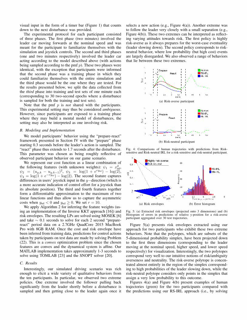
enough to elicit a wide variety of qualitative behaviors fromthe ten participants. In particular, we observed two extremepolicies. One extreme involved the follower pulling backsignificantly from the leader shortly before a disturbance issampled and then getting close to the leader again once it

selects a new action (e.g., Figure 4(a)). Another extreme wasto follow the leader very closely with a small separation (e.g.,Figure 4(b)). These two extremes can be interpreted as reflect-ing varying attitudes towards risk. The first policy is highlyrisk-averse as it always prepares for the worst-case eventuality(leader slowing down). The second policy corresponds to risk-neutral behavior, where low probability (but high cost) eventsare largely disregarded. We also observed a range of behaviorsthat lie between these two extremes.

(a) Risk-averse participant

(b) Risk-neutral participant

Fig. 4: Comparisons of human trajectories with predictions from Risk-sensitive and Risk-neutral IRL for a risk-sensitive and risk-neutral participant.

(a) Risk envelopes (b) Error histogram

Fig. 5: (a) Extracted risk envelopes (projected onto 3 dimensions) and (b)Histogram of errors in predictions of relative y-position for a risk-averseparticipant aggregated over 30 test trajectories.

Figure 5(a) presents risk envelopes extracted using ourapproach for two participants who exhibit these two extremebehaviors. Note that the polytopes, which are subsets of the5-dimensional probability simplex, have been projected downto the first three dimensions (corresponding to the leadermoving at the nominal speed, higher speed, and lower speedrespectively) for visualization. Interestingly, the two polytopescorrespond very well to our intuitive notions of risk/ambiguityaverseness and neutrality. The risk-averse polytope is concen-trated almost entirely in the region of the simplex correspond-ing to high probabilities of the leader slowing down, while therisk-neutral polytope considers only points in the simplex thatassign a very low probability to this outcome.

Figures 4(a) and Figure 4(b) present examples of humantrajectories (green) for the two participants compared withthe predictions using our RS-IRL approach (i.e., by solving

problem (22) using the inferred cost function and polytope) fora single 2 second prepare-react period. We see that our RS-IRLapproach reproduces the qualitatively different driving stylesof the two participants. For the risk-averse participant, thepredicted trajectory backs off the leader car in the “prepare”stage and moves close again once the leader chooses itsaction. For the risk-neutral participant, the predicted trajectoryremains in close proximity to the leader at all times.

Figure 4 also compares the RS-IRL approach with onewhere the expert is modeled as minimizing the expected valueof his/her cost function computed with respect to the pmfp. Since this risk-neutrality is the standard assumption madeby traditional IRL approaches, it constitutes an importantbenchmark for comparison. We refer to this approach as risk-neutral IRL (RN-IRL). The predicted trajectories (blue) usingthis model are generated by solving Problem (20) with therisk operator ρ replaced by the expected value. As one wouldexpect, the predictions using RS-IRL and RN-IRL are similarfor the risk-neutral participant (Figure 4(b)). However, asFigure 4(a) demonstrates, the RN-IRL model does not predictthe significant backing off behavior exhibited by the humanand significantly underestimates yrel over the 2 second period.

Figure 5(b) plots a histogram of errors (ypredictedrel,k −yhumanrel,k )(k = 0, ..., 20) for the predictions made by RS-IRL and RN-IRL computed for all 30 trajectories in our test set for therisk-averse participant. We observe that RN-IRL significantlyunderestimates yrel, while the RS-IRL approach makes notice-ably more accurate predictions. However, we note that RS-IRL still exhibits a slight bias towards under-predicting yrel.This is because the risk-averse participant consistently backsoff the leader car by a very large amount (as observed inFigure 4(a)), which may be explained by the fact that whileour model assumes that the expert has an exact knowledgeof the magnitudes of the disturbances/speeds in the set W ,this is only approximately true in reality (especially since theparticipants experienced the low speed setting quite rarely inthe training phase). Thus, one would expect a more significantbacking off maneuver if the participant overestimates thedifference in the nominal and slow leader speed settings. Thisissue could potentially be dealt with by considering additional“spurious” disturbance settings (e.g., introducing a lower speedsetting in W) when applying our RS-IRL approach.

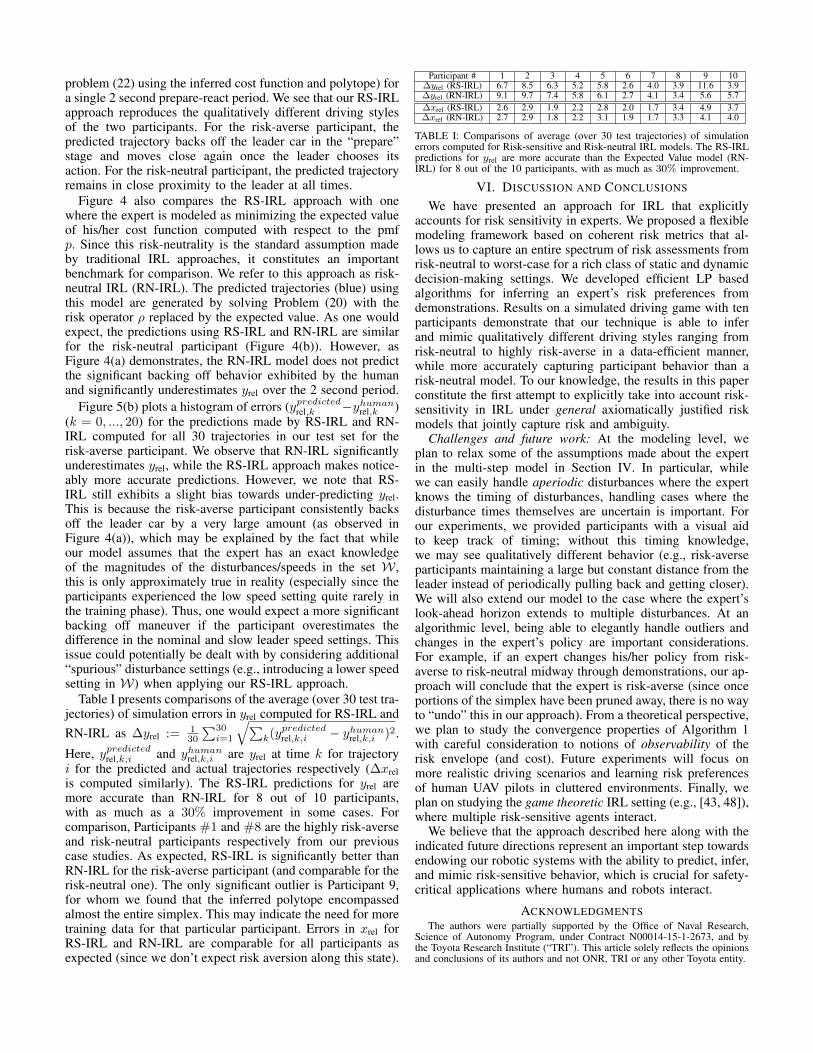
Table I presents comparisons of the average (over 30 test tra-jectories) of simulation errors in yrel computed for RS-IRL andRN-IRL as ∆yrel := 1

30

∑30i=1

√∑k(ypredictedrel,k,i − yhumanrel,k,i )2.

Here, ypredictedrel,k,i and yhumanrel,k,i are yrel at time k for trajectoryi for the predicted and actual trajectories respectively (∆xrelis computed similarly). The RS-IRL predictions for yrel aremore accurate than RN-IRL for 8 out of 10 participants,with as much as a 30% improvement in some cases. Forcomparison, Participants #1 and #8 are the highly risk-averseand risk-neutral participants respectively from our previouscase studies. As expected, RS-IRL is significantly better thanRN-IRL for the risk-averse participant (and comparable for therisk-neutral one). The only significant outlier is Participant 9,for whom we found that the inferred polytope encompassedalmost the entire simplex. This may indicate the need for moretraining data for that particular participant. Errors in xrel forRS-IRL and RN-IRL are comparable for all participants asexpected (since we don’t expect risk aversion along this state).

Participant # 1 2 3 4 5 6 7 8 9 10∆yrel (RS-IRL) 6.7 8.5 6.3 5.2 5.8 2.6 4.0 3.9 11.6 3.9∆yrel (RN-IRL) 9.1 9.7 7.4 5.8 6.1 2.7 4.1 3.4 5.6 5.7∆xrel (RS-IRL) 2.6 2.9 1.9 2.2 2.8 2.0 1.7 3.4 4.9 3.7∆xrel (RN-IRL) 2.7 2.9 1.8 2.2 3.1 1.9 1.7 3.3 4.1 4.0

TABLE I: Comparisons of average (over 30 test trajectories) of simulationerrors computed for Risk-sensitive and Risk-neutral IRL models. The RS-IRLpredictions for yrel are more accurate than the Expected Value model (RN-IRL) for 8 out of the 10 participants, with as much as 30% improvement.

VI. DISCUSSION AND CONCLUSIONS

We have presented an approach for IRL that explicitlyaccounts for risk sensitivity in experts. We proposed a flexiblemodeling framework based on coherent risk metrics that al-lows us to capture an entire spectrum of risk assessments fromrisk-neutral to worst-case for a rich class of static and dynamicdecision-making settings. We developed efficient LP basedalgorithms for inferring an expert’s risk preferences fromdemonstrations. Results on a simulated driving game with tenparticipants demonstrate that our technique is able to inferand mimic qualitatively different driving styles ranging fromrisk-neutral to highly risk-averse in a data-efficient manner,while more accurately capturing participant behavior than arisk-neutral model. To our knowledge, the results in this paperconstitute the first attempt to explicitly take into account risk-sensitivity in IRL under general axiomatically justified riskmodels that jointly capture risk and ambiguity.

Challenges and future work: At the modeling level, weplan to relax some of the assumptions made about the expertin the multi-step model in Section IV. In particular, whilewe can easily handle aperiodic disturbances where the expertknows the timing of disturbances, handling cases where thedisturbance times themselves are uncertain is important. Forour experiments, we provided participants with a visual aidto keep track of timing; without this timing knowledge,we may see qualitatively different behavior (e.g., risk-averseparticipants maintaining a large but constant distance from theleader instead of periodically pulling back and getting closer).We will also extend our model to the case where the expert’slook-ahead horizon extends to multiple disturbances. At analgorithmic level, being able to elegantly handle outliers andchanges in the expert’s policy are important considerations.For example, if an expert changes his/her policy from risk-averse to risk-neutral midway through demonstrations, our ap-proach will conclude that the expert is risk-averse (since onceportions of the simplex have been pruned away, there is no wayto “undo” this in our approach). From a theoretical perspective,we plan to study the convergence properties of Algorithm 1with careful consideration to notions of observability of therisk envelope (and cost). Future experiments will focus onmore realistic driving scenarios and learning risk preferencesof human UAV pilots in cluttered environments. Finally, weplan on studying the game theoretic IRL setting (e.g., [43, 48]),where multiple risk-sensitive agents interact.

We believe that the approach described here along with theindicated future directions represent an important step towardsendowing our robotic systems with the ability to predict, infer,and mimic risk-sensitive behavior, which is crucial for safety-critical applications where humans and robots interact.

ACKNOWLEDGMENTSThe authors were partially supported by the Office of Naval Research,

Science of Autonomy Program, under Contract N00014-15-1-2673, and bythe Toyota Research Institute (“TRI”). This article solely reflects the opinionsand conclusions of its authors and not ONR, TRI or any other Toyota entity.

REFERENCES

[1] P. Abbeel and A. Y. Ng. Apprenticeship learning viainverse reinforcement learning. In Int. Conf. on MachineLearning, 2004.

[2] P. Abbeel and A. Y. Ng. Exploration and apprenticeshiplearning in reinforcement learning. In Int. Conf. onMachine Learning, 2005.

[3] C. Acerbi. Spectral measures of risk: A coherent repre-sentation of subjective risk aversion. Journal of Banking& Finance, 26(7):1505–1518, 2002.

[4] C. Acerbi and D. Tasche. On the coherence of expectedshortfall. Journal of Banking & Finance, 26(7):1487–1503, 2002.

[5] Maurice Allais. Le comportement de lhomme rationneldevant le risque: critique des postulats et axiomes delecole americaine. Econometrica, 21(4):503–546, 1953.

[6] MOSEK ApS. MOSEK optimization software. Availableat https://mosek.com/.

[7] P. Artzner, F. Delbaen, J.-M. Eber, and D. Heath. Co-herent measures of risk. Mathematical Finance, 9(3):203–228, 1999.

[8] A. Axelrod, L. Carlone, G. Chowdhary, and S. Karaman.Data-driven prediction of EVAR with confidence in time-varying datasets. In IEEE Conf. on Decision and Control,2016.

[9] N. C. Barberis. Thirty years of prospect theory in eco-nomics: A review and assessment. Journal of EconomicPerspectives, 27(1):173–195, 2013.

[10] N. Bauerle and J. Ott. Markov decision processes withaverage-value-at-risk criteria. Mathematics of OperationsResearch, 74(3):361–379, 2011.

[11] D. Carton, V. Nitsch, D. Meinzer, and D. Wollherr. To-wards assessing the human trajectory planning horizon.PLoS ONE, 11(12):e0167021, 2016.

[12] Y. Chow and M. Pavone. A framework for time-consistent, risk-averse model predictive control: Theoryand algorithms. In American Control Conference, June2014.

[13] Y. Chow, A. Tamar, S. Mannor, and M. Pavone. Risk-sensitive and robust decision-making: a CVaR optimiza-tion approach. In Advances in Neural InformationProcessing Systems, 2015.

[14] A. Eichhorn and W. Romisch. Polyhedral risk measuresin stochastic programming. SIAM Journal on Optimiza-tion, 16(1):69–95, 2005.

[15] D. Ellsberg. Risk, ambiguity, and the savage axioms. TheQuarterly Journal of Economics, 75(4):643–669, 1961.

[16] P. Englert and M. Toussaint. Inverse KKT learning costfunctions of manipulation tasks from demonstrations. InInt. Symp. on Robotics Research, 2015.

[17] J. A. Filar, L. C. M. Kallenberg, and H.-M. Lee.Variance-penalized Markov decision processes. Math-ematics of Operations Research, 14(1):147–161, 1989.

[18] I. Gilboa and M. Marinacci. Ambiguity and the Bayesianparadigm. In Readings in Formal Epistemology, chap-ter 21. First edition, 2016.

[19] I. Gilboa and D. Schmeidler. Maxmin expected utilitywith non-unique prior. Journal of Mathematical Eco-nomics, 18(2):141–153, 1989.

[20] P. E. Gill, W. Murray, and M. A. Saunders. SNOPT: An

SQP algorithm for large-scale constrained optimization.SIAM Review, 47(1):99–131, 2005.

[21] P.W. Glimcher and E. Fehr. Neuroeconomics. Elsevier,second edition, 2014.

[22] J. D. Hey, G. Lotito, and A. Maffioletti. The descriptiveand predictive adequacy of theories of decision makingunder uncertainty/ambiguity. Journal of Risk and Uncer-tainty, 41(2):81–111, 2010.

[23] K. Holmstrom and M. M. Edvall. The TOMLABoptimization environment. In Modeling Languages inMathematical Optimization. 2004.

[24] R. Howard and J. Matheson. Risk-sensitive Markovdecision processes. Management Science, 8(7):356–369,1972.

[25] M. Hsu, M. Bhatt, R. Adolphs, D. Tranel, and C. F.Camerer. Neural systems responding to degrees ofuncertainty in human decision-making. Science, 310(5754):1680–1683, 2005.

[26] Daniel Kahneman and Amos Tversky. Prospect theory:An analysis of decision under risk. Econometrica, pages263–291, 1979.

[27] J. Z. Kolter, P. Abbeel, and A. Y. Ng. Hierarchicalapprenticeship learning with application to quadruped lo-comotion. In Advances in Neural Information ProcessingSystems, 2007.

[28] M. Kuderer, S. Gulati, and W. Burgard. Learning drivingstyles for autonomous vehicles from demonstration. InProc. IEEE Conf. on Robotics and Automation, 2015.

[29] S. Levine and V. Koltun. Continuous inverse optimalcontrol with locally optimal examples. In Int. Conf. onMachine Learning, 2012.

[30] O. Mihatsch and R. Neuneier. Risk-sensitive reinforce-ment learning. Machine Learning, 49(2):267–290, 2002.

[31] K. Mombaur, A. Truong, and J.-P Laumond. Fromhuman to humanoid locomotion—an inverse optimalcontrol approach. Autonomous Robots, 28(3):369–383,2010.

[32] A. Ng and S.J. Russell. Algorithms for inverse reinforce-ment learning. In Int. Conf. on Machine Learning, 2000.

[33] A. Nilim and L. El Ghaoui. Robust control of Markovdecision processes with uncertain transition matrices.Operations Research, 53(5):780–798, 2005.

[34] T. Osogami. Robustness and risk-sensitivity in Markovdecision processes. In Advances in Neural InformationProcessing Systems, 2012.

[35] T. Park and S. Levine. Inverse optimal control forhumanoid locomotion. In Robotics: Science and Sys-tems Workshop on Inverse Optimal Control and RoboticLearning from Demonstration, 2013.

[36] M. Petrik and D. Subramanian. An approximate solutionmethod for large risk-averse Markov decision processes.In Proc. Conf. on Uncertainty in Artificial Intelligence,2012.

[37] M. Rabin. Risk aversion and expected-utility theory:A calibration theorem. Econometrica, 68(5):1281–1292,2000.

[38] D. Ramachandran and E. Amir. Bayesian inverse rein-forcement learning. In Proc. Int. Conf. on AutonomousAgents and Multiagent Systems, 2007.

[39] R. T. Rockafellar. Coherent approaches to risk inoptimization under uncertainty. In OR Tools and Ap-

plications: Glimpses of Future Technologies, chapter 3.INFORMS, 2007.

[40] R. T. Rockafellar and S. Uryasev. Optimization ofconditional value-at-risk. Journal of Risk, 2:21–41, 2000.

[41] S. Russell. Learning agents for uncertain environments.In Proc. Computational Learning Theory, 1998.

[42] A. Ruszczynski. Risk-averse dynamic programming forMarkov decision process. Mathematical Programming,125(2):235–261, 2010.

[43] D. Sadigh, S. Sastry, S. A. Seshia, and A. D. Dragan.Planning for autonomous cars that leverage effects onhuman actions. In Robotics: Science and Systems, 2016.

[44] A. Shapiro. On a time consistency concept in riskaverse multi-stage stochastic programming. OperationsResearch Letters, 37(3):143–147, 2009.

[45] Y. Shen, M. J. Tobia, T. Sommer, and K. Obermayer.Risk-sensitive reinforcement learning. Neural Computa-tion, 26(7):1298–1328, 2014.

[46] A. Tamar, D. Di Castro, and S. Mannor. Policy gradientswith variance related risk criteria. In Int. Conf. onMachine Learning, 2012.

[47] J. von Neumann and O. Morgenstern. Theory of Gamesand Economic Behavior. Princeton University Press,1944.

[48] Kevin Waugh, Brian D. Ziebart, and J. Andrew Bagnell.Computational rationalization: The inverse equilibriumproblem. In Int. Conf. on Machine Learning, 2011.

[49] H. Xu and S. Mannor. Distributionally robust Markovdecision processes. In Advances in Neural InformationProcessing Systems, 2010.

[50] B. D. Ziebart, A. Maas, J. A. Bagnell, and A. K. Dey.Maximum entropy inverse reinforcement learning. InProc. AAAI Conf. on Artificial Intelligence, 2008.

[51] B. D. Ziebart, N. Ratliff, G. Gallagher, C. Mertz, K. Pe-terson, J. A. Bagnell, M. Hebert, A. K. Key, and S. Srini-vasa. Planning-based prediction for pedestrians. InIEEE/RSJ Int. Conf. on Intelligent Robots & Systems,2009.

[52] M. Zucker, J. A. Bagnell, C. G. Atkeson, and J. Kuffner.An optimization approach to rough terrain locomotion.In Proc. IEEE Conf. on Robotics and Automation, 2010.