Chapter 7

An investment’s return is your reward for investing.

An investment’s risk is the uncertainty of what will happen with your investment dollar.

The relationship between risk and return is a tradeoff. The more risk you are willing to take, the higher the potential return (and vice versa).

18%

16%

14%

12%

10%

8%

6%

4%

2%

0% 5% 10% 15% 20% 25% 30% 35%

T-billsT-bonds

Large-cap stocks

Small-cap stocks

Retu

rn

Risk (Annual standard deviation of return)

A dollar return is the return on an investment measured in actual dollars.

This return has two components: ◦ Cash you receive while you own the investment. ◦ The value of the asset you purchase may change.

Capital gain or capital loss

Example: Suppose you buy 100 shares of Allstate Corp (ALL) on January 1. At the time, ALL was selling for $58.50/share. ◦ At the end of the year, you want to see how much you

made.

Over the year, Allstate pays dividends of $1.20 per share. By the end of the year, you received: ◦ Dividend income = $1.20 × 100 = $120

Suppose on Dec 31, Allstate was selling for $67.80 meaning the value of your stock increased by $9.30 per share ◦ Capital gain = ($67.80 - $58.50) X 100 = $930

Total dollar return = $120 + $930 = $1,050

How much do we get for each dollar we invest?

◦ Let Pt be the price of the stock at the beginning of the year and let Dt+1 be the dividend paid during the year.

Dividend yield = $1.20 / $58.50 = .02051 For each dollar invested, ALL paid a little over 2₵ in

dividends.

Capital gains yield = ($67.80 - $58.50) / $58.50 = .15897

For each dollar invested, ALL paid out almost 16₵ in capital gains.

Total percentage return = .02051 + .15897 = .17949 (17.95%)

For each dollar invested, ALL paid out 17.95₵ in total. (referred to as the rate of return)

You don’t always hold a security for exactly one year.

We need to do a little more work to make returns comparable by annualizing them, but we will start with HPR.

Suppose you buy 200 shares of Lowe’s (LOW) at $48/share. In three months, you sell it at $51. You collect no dividends…

HPR = (Pt+1 – Pt)/Pt = $3/$48 = .0625

The 6.25% is your return for your 3-month holding period, but what does this amount to on a per-year basis? We need the effective annual return.

1 + EAR = (1 + HPR)ⁿ ◦ where ⁿ is the number of holding periods in a year.

1 + EAR = (1+ .0625)⁴ = 1.2744

The annualized return is 27.44%

In order to calculate an annualized return of an investment held more than one year, the same formula for EAR is used.

However, in the case of a multiple year HPR, the “n” in the formula must be made into a fraction of one divided by the number of years the asset has been held.

◦ For instance, to calculate the annualized return for an asset held for three years, the “n” would be 1/3 (or 0.33333).

◦ What if the HPR was 6 years and 3 months? The “n” would be 1/6.25 (or 0.16).

Thus far, you have calculated an average annualized return; however, average returns can actually be calculated two different ways. ◦ The geometric average ◦ The arithmetic average

As an example: ◦ Assume that you purchase an investment for $1,000 and

over the course of one year; the investment loses half of its value (falling to $500). However, you continue to hold the investment for another year, in which the investment enjoys returns that take it back to $1,000. What is the annualized return?

The geometric average answers the question: What was the average compound return per year over a particular period?

1 + EAR = (1 + 0.00)1/2 = 0.00%

The arithmetic average answers the question: What was the return in an average year over a particular period?

Average return = (-50% + 100%) / 2 = 25%

What is the geometric and arithmetic average for an investment with the following annual returns?

◦ Year 1 = 9%

◦ Year 2 = -14%

◦ Year 3 = 22%

◦ Year 4 = 6%

Geometric average = (1.09 × .86 × 1.22 × 1.06)1/4 = 1.0493 – 1 = 0.0493 = 4.93%

Arithmetic average = (.09 + -.14 + .22 + .06) / 4 = 5.75%

It depends on the question you are trying to answer. Further consider:

The arithmetic average assumes independence of variables and can be overly optimistic (especially for longer-term holdings).

The geometric average assumes dependence of variables and can be overly pessimistic (especially for shorter-term holdings).

Your personal investment returns are typically dependent. ◦ If your investment gains (loses) value, then you have more (less)

money to generate future returns.

Most investment companies only report the arithmetic average when reporting performance.

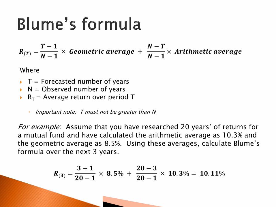
Where

T = Forecasted number of years N = Observed number of years RT = Average return over period T

◦ Important note: T must not be greater than N

𝑹(𝑻) =𝑻 − 𝟏

𝑵 − 𝟏 × 𝑮𝒆𝒐𝒎𝒆𝒕𝒓𝒊𝒄 𝒂𝒗𝒆𝒓𝒂𝒈𝒆 +

𝑵 − 𝑻

𝑵− 𝟏× 𝑨𝒓𝒊𝒕𝒉𝒎𝒆𝒕𝒊𝒄 𝒂𝒗𝒆𝒓𝒂𝒈𝒆

For example: Assume that you have researched 20 years’ of returns for a mutual fund and have calculated the arithmetic average as 10.3% and the geometric average as 8.5%. Using these averages, calculate Blume’s formula over the next 3 years.

𝑹(𝟑) =𝟑 − 𝟏

𝟐𝟎 − 𝟏 × 𝟖. 𝟓% +

𝟐𝟎 − 𝟑

𝟐𝟎 − 𝟏 × 𝟏𝟎. 𝟑% = 𝟏𝟎. 𝟏𝟏%

While knowing the “average” return on an investment is helpful, it provides you with no insight into the dispersion of returns.

This dispersion of return is the basic measure for risk in an investment.

Another term used to describe a single investment’s risk is its “volatility”. ◦ In finance, volatility is a measure of the variation of

a security’s price over time and it is measured by the dispersion of returns for a given security or index.

If we are unwilling to bear any risk at all, but are willing to forgo the use of our money for a while, then we can earn the risk-free rate. ◦ The time value of money

If we are willing to bear risk, then we can expect to earn a risk premium (a return in excess of the risk-free rate).

The risk premium is the compensation for investors who tolerate extra risk (typically higher the risk premium – the more volatile the investment).

Volatility is calculating by an investment’s variance.

𝝈𝟐 = (𝑿 − 𝝁)

𝟐

𝐍

Where σ2 = Variance X = Individual return observation µ = Mean return N = Number of observations

“Variance”, by itself, is difficult to interpret.

The standard deviation (the square root of the variance) provides much more insight on the investment’s volatility.

A volatile security will have a high standard deviation whereas a stable security will generally have a much lower standard deviation.

Standard deviation (𝛔) = 𝝈𝟐

Suppose we do some research, and discover the historical returns of a mutual fund based on economic conditions. Further we are able to estimate the chances of the economic conditions in any given year.

◦ In a severe recession, the fund’s return is -22%

◦ In a mild recession, the fund’s return is -5%

◦ In a normal growth period, the fund’s return is 16%

◦ In an exceptional growth period, the fund’s return is 24%

◦ There is a 5% probability of a severe recession

◦ There is a 30% probability of a mild recession

◦ There is a 50% probability of normal growth

◦ There is a 15% probability of exceptional growth

Probability ×

Scenario Probability HPR (%) HPR

Severe recession 0.05 -22 -1.10

Mild recession 0.30 -5 -1.50

Normal growth 0.50 16 8.00

Exceptional growth 0.15 24 3.60

Expected return: 9.00%

Difference Squared deviation

Probability HPR µ (HPR - µ) Squared deviation × Probability

0.05 -22 9 -31.00 961.00 48.05

0.30 -5 9 -14.00 196.00 58.80

0.50 16 9 7.00 49.00 24.50

0.15 24 9 15.00 225.00 33.75

Variance: 165.1

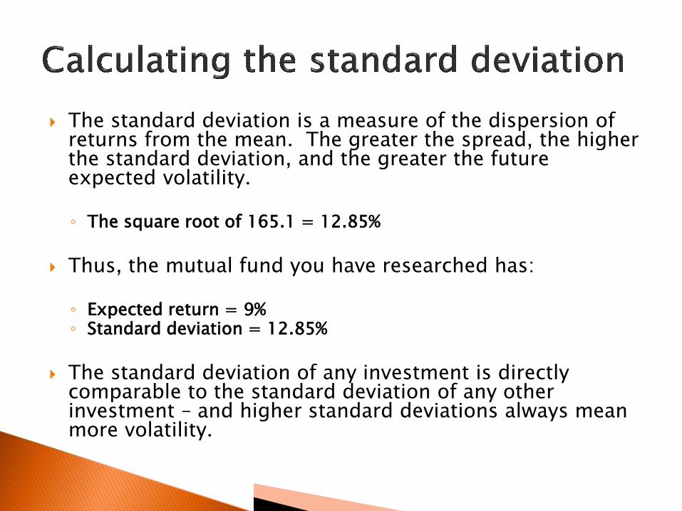
The standard deviation is a measure of the dispersion of returns from the mean. The greater the spread, the higher the standard deviation, and the greater the future expected volatility.

◦ The square root of 165.1 = 12.85%

Thus, the mutual fund you have researched has: ◦ Expected return = 9% ◦ Standard deviation = 12.85%

The standard deviation of any investment is directly

comparable to the standard deviation of any other investment – and higher standard deviations always mean more volatility.

-29.6% -16.7% -3.9% 9% 21.9% 34.7% 47.6%

The mean is the average return we expect

given all of the different possible outcomes.

Variance and standard deviation give us a

quantitative measurement of the level of

dispersion of the possible outcomes.

Only 2.6 observations

out of 1,000 fall outside

3SDs

Our investment has an expected return of 9% and a standard deviation of 12.85%.

In any given year, we can be reasonably certain that:

◦ 68.26% of outcomes will fall within one standard deviation

◦ 95.44% of outcomes will fall within two standard deviations

◦ 99.74% of outcomes will fall within three standard deviations

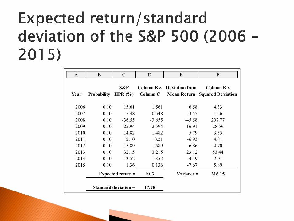
A B C D E F

S&P Column B × Deviation from Column B ×

Year Probability HPR (%) Column C Mean Return Squared Deviation

2006 0.10 15.61 1.561 6.58 4.33

2007 0.10 5.48 0.548 -3.55 1.26

2008 0.10 -36.55 -3.655 -45.58 207.77

2009 0.10 25.94 2.594 16.91 28.59

2010 0.10 14.82 1.482 5.79 3.35

2011 0.10 2.10 0.21 -6.93 4.81

2012 0.10 15.89 1.589 6.86 4.70

2013 0.10 32.15 3.215 23.12 53.44

2014 0.10 13.52 1.352 4.49 2.01

2015 0.10 1.36 0.136 -7.67 5.89

Expected return = 9.03 Variance = 316.15

Standard deviation = 17.78

A B C D E F

Rus 2000 Column B × Deviation from Column B ×

Year Probability HPR (%) Column C Mean Return Squared Deviation

2006 0.10 17.00 1.7 17.00 28.90

2007 0.10 -2.75 -0.275 -2.75 0.76

2008 0.10 -34.80 -3.48 -34.80 121.10

2009 0.10 25.22 2.522 25.22 63.60

2010 0.10 25.31 2.531 25.31 64.06

2011 0.10 -5.45 -0.545 -5.45 2.97

2012 0.10 14.63 1.463 14.63 21.40

2013 0.10 37.00 3.7 37.00 136.90

2014 0.10 3.53 0.353 3.53 1.25

2015 0.10 -5.71 -0.571 -5.71 3.26

Expected return = 7.40 Variance = 444.21

Standard deviation = 21.08

What if a comparison of two stocks yielded the following?

◦ Stock X has an expected return of 15% and a standard deviation of 10%.

◦ Stock Y has an expected return of 13% and a standard deviation of 8%.

To aid investors in making decisions between securities with different expected returns, one might apply an additional tool known as the coefficient of variation (CV).

CV = Standard deviation / Expected return

The CV considers how much volatility you are assuming in comparison to the level of return you expect from the investment.

◦ The higher the CV, the greater the risk.

The CV for Stock X = .10 / .15 = .67

The CV for Stock Y = .08 / .13 = .62

The rational risk-averse investor would not deem the higher return of Stock X to be worth the extra risk, relative to Stock Y.

Investors can choose to hold risky and riskless assets.

But how much should you put in each one? ◦ The weights will be determined by your risk level

and the risk/return tradeoff.

Example: rf = 4% rf = 4% srf = 0% srf = 0%

E(rp) = 9% E(rp) = 9% srp = 12% srp = 12%

100% in the

risky asset

100% in the

risk-free rate

Capital Allocation Line

ơ

Re

turn

The investor could potentially choose to invest 100% of their assets into the risk-free rate or 100% of their assets into the risky asset, or any combination in between.

What is the expected return and standard deviation of a portfolio that consists of 60% of assets invested into the balanced index fund and 40% of assets invested in the risk free rate?

ER(p60/40) = (.60 × .09) + (.40 × .04) ER(p60/40) = .07 The expected return of a 60/40 combination is 7% Ơ(p60/40) = (.60 × .12) + (.40 × 0.0) Ơ(p60/40) = .072 The standard deviation of a 60/40 combination is

7.2%

What if instead of a 60/40 combination of the balanced fund and the risk-free rate, a 30/70 combination is used?

ER(p30/70) = (.30 × .09) + (.70 × .04) ER(p30/70) = .055 The expected return of a 30/70 combination is

5.5% Ơ(p30/70) = (.30 × .12) + (.70 × 0.0) Ơ(p30/70) = .036 The standard deviation of a 30/70 combination

is 3.6%

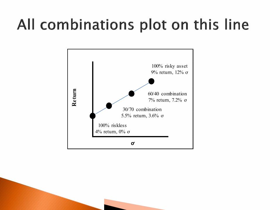
100% risky asset

9% return, 12% ơ

ơ

Re

turn

100% riskless

4% return, 0% ơ

30/70 combination

5.5% return, 3.6% ơ

60/40 combination

7% return, 7.2% ơ

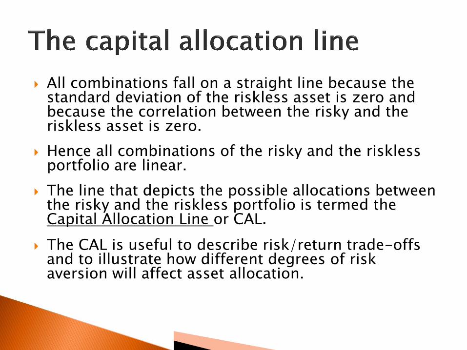
All combinations fall on a straight line because the standard deviation of the riskless asset is zero and because the correlation between the risky and the riskless asset is zero.

Hence all combinations of the risky and the riskless portfolio are linear.

The line that depicts the possible allocations between the risky and the riskless portfolio is termed the Capital Allocation Line or CAL.

The CAL is useful to describe risk/return trade-offs and to illustrate how different degrees of risk aversion will affect asset allocation.

Using a margin account, investors can borrow at a rate not statistically indifferent from the risk-free rate.

What would be the expected return and standard

deviation of a portfolio that invests 150% in the risky asset?

◦ ER(p150) = (1.50 × .09) + (-.50 × .04) ◦ ER(p150) = .115 ◦ The expected return of a levered 150% portfolio is 11.5%

◦ Ơ(p150) = (1.50 × .12) + (-.50 × 0.0) ◦ Ơ(p150) = .18 ◦ The standard deviation of a levered 150% portfolio is 18%

Given that the investor is able to borrow at the risk-free rate, the formula for calculating the return and standard deviation works to (in essence) extend the capital allocation line.

100% risky asset

9% return, 12% ơ

ơ

Re

turn

100% riskless

4% return, 0% ơ

150% risky asset

11.5% return, 18% ơ