Risk Premiums in Dynamic Term Structure Models with ...sjoslin/papers/JPS_JF.pdf · Risk Premiums...
37
THE JOURNAL OF FINANCE • VOL. LXIX, NO. 3 • JUNE 2014 Risk Premiums in Dynamic Term Structure Models with Unspanned Macro Risks SCOTT JOSLIN, MARCEL PRIEBSCH, and KENNETH J. SINGLETON ∗ ABSTRACT This paper quantifies how variation in economic activity and inflation in the United States influences the market prices of level, slope, and curvature risks in Treasury markets. We develop a novel arbitrage-free dynamic term structure model in which bond investment decisions are influenced by output and inflation risks that are un- spanned by (imperfectly correlated with) information about the shape of the yield curve. Our model reveals that, between 1985 and 2007, these risks accounted for a large portion of the variation in forward terms premiums, and there was pronounced cyclical variation in the market prices of level and slope risks. A POWERFUL IMPLICATION of virtually all macro-finance affine term structure models (MTSMs)—reduced-form and equilibrium alike—is that the macro fac- tors that determine bond prices are fully spanned by the current yield curve. 1 That is, the affine mapping between bond yields and the risks in the macroe- conomy in these models can be inverted to express these risk factors as lin- ear combinations of yields. This theoretical macro-spanning condition implies strong and often counterfactual restrictions on the joint distribution of bond yields and the macroeconomy, as well as on how macroeconomic shocks affect term premiums. Consider, for instance, an MTSM in which the macro variables M t that di- rectly determine bond yields are output growth and inflation. Macro spanning implies that these macro variables can be replicated by portfolios of bond yields. ∗ Joslin is with the University of Southern California, Marshall School of Business. Priebsch is with the Federal Reserve Board. Singleton is with Stanford University, Graduate School of Business and NBER. We are grateful for feedback from seminar participants at MIT, Stanford University, the University of Chicago, the Federal Reserve Board and Federal Reserve Bank of San Francisco, the International Monetary Fund, and the Western Finance Association (San Diego), and for comments from Greg Duffee, Patrick Gagliardini, Imen Ghattassi, Monika Piazzesi, Oreste Tristani, and Jonathan Wright. An earlier version of this paper was circulated under the title “Risk Premium Accounting in Macro-Dynamic Term Structure Models.” The analysis and conclusions set forth in this paper are those of the authors and do not indicate concurrence by other members of the research staff or the Board of Governors of the Federal Reserve System. 1 Reduced-form models that enforce theoretical spanning include Ang and Piazzesi (2003), Ang, Dong, and Piazzesi (2007), Rudebusch and Wu (2008), Ravenna and Sepp ¨ al¨ a(2008), Smith and Taylor (2009), and Bikbov and Chernov (2010). In many equilibrium models with long-run risks (e.g., Bansal, Kiku, and Yaron (2012a), Bansal and Shaliastovich (2013)), it is expected consumption growth and expected inflation that are spanned by yields. DOI: 10.1111/jofi.12131 1197
Transcript of Risk Premiums in Dynamic Term Structure Models with ...sjoslin/papers/JPS_JF.pdf · Risk Premiums...

THE JOURNAL OF FINANCE • VOL. LXIX, NO. 3 • JUNE 2014
Risk Premiums in Dynamic Term StructureModels with Unspanned Macro Risks
SCOTT JOSLIN, MARCEL PRIEBSCH, and KENNETH J. SINGLETON∗
ABSTRACT
This paper quantifies how variation in economic activity and inflation in the UnitedStates influences the market prices of level, slope, and curvature risks in Treasurymarkets. We develop a novel arbitrage-free dynamic term structure model in whichbond investment decisions are influenced by output and inflation risks that are un-spanned by (imperfectly correlated with) information about the shape of the yieldcurve. Our model reveals that, between 1985 and 2007, these risks accounted for alarge portion of the variation in forward terms premiums, and there was pronouncedcyclical variation in the market prices of level and slope risks.
A POWERFUL IMPLICATION of virtually all macro-finance affine term structuremodels (MTSMs)—reduced-form and equilibrium alike—is that the macro fac-tors that determine bond prices are fully spanned by the current yield curve.1
That is, the affine mapping between bond yields and the risks in the macroe-conomy in these models can be inverted to express these risk factors as lin-ear combinations of yields. This theoretical macro-spanning condition impliesstrong and often counterfactual restrictions on the joint distribution of bondyields and the macroeconomy, as well as on how macroeconomic shocks affectterm premiums.
Consider, for instance, an MTSM in which the macro variables Mt that di-rectly determine bond yields are output growth and inflation. Macro spanningimplies that these macro variables can be replicated by portfolios of bond yields.
∗Joslin is with the University of Southern California, Marshall School of Business. Priebschis with the Federal Reserve Board. Singleton is with Stanford University, Graduate School ofBusiness and NBER. We are grateful for feedback from seminar participants at MIT, StanfordUniversity, the University of Chicago, the Federal Reserve Board and Federal Reserve Bank of SanFrancisco, the International Monetary Fund, and the Western Finance Association (San Diego),and for comments from Greg Duffee, Patrick Gagliardini, Imen Ghattassi, Monika Piazzesi, OresteTristani, and Jonathan Wright. An earlier version of this paper was circulated under the title “RiskPremium Accounting in Macro-Dynamic Term Structure Models.” The analysis and conclusionsset forth in this paper are those of the authors and do not indicate concurrence by other membersof the research staff or the Board of Governors of the Federal Reserve System.
1 Reduced-form models that enforce theoretical spanning include Ang and Piazzesi (2003), Ang,Dong, and Piazzesi (2007), Rudebusch and Wu (2008), Ravenna and Seppala (2008), Smith andTaylor (2009), and Bikbov and Chernov (2010). In many equilibrium models with long-run risks(e.g., Bansal, Kiku, and Yaron (2012a), Bansal and Shaliastovich (2013)), it is expected consumptiongrowth and expected inflation that are spanned by yields.
DOI: 10.1111/jofi.12131
1197

1198 The Journal of Finance R©
As a result, after conditioning on the current yield curve, macro variables areuninformative about both expected excess returns (risk premiums) and futurevalues of M. The first of these restrictions on the joint distribution of M andbond yields is contradicted by the evidence in Cooper and Priestley (2008) andLudvigson and Ng (2010). The second is contradicted by a large body of evidenceon forecasting the business cycle (Stock and Watson (2003)). Both restrictionsare strongly rejected statistically in our data set.
There is an equally compelling conceptual case for relaxing macro spanning.The first three principal components (PCs) of bond yields—the level, slope,and curvature—explain almost all of the variation in yields, and this fact moti-vates the small number of risk factors in reduced-form MTSMs.2 Real economicgrowth in the U.S. economy is a distinct agglomeration of a high-dimensionalset of risks from financial, product, and labor markets. The yield PCs are cor-related with output growth, but the natural premise in economic modeling issurely that the portfolio of risks that shape growth are not spanned by the PCsof U.S. Treasury yields. In fact, in our data, only about 30% of the variation inoutput growth is spanned by even the first five PCs of yields.
In this paper, we develop a family of reduced-form Gaussian MTSMs that al-lows for macroeconomic risks that are unspanned by the yield curve and therebyintroduces macroeconomic risks that are distinct from PC (yield curve) risks.Central to the construction of our MTSM are the assumptions that the pricingkernel investors use when discounting cash flows depends on a comprehensiveset of priced risks Zt in the macroeconomy, and the short-term Treasury rateis an affine function of a smaller set of “portfolios” of these risks Xt (consistentwith the evidence that a small number of PCs explain most of the variationin the cross section of yields). We then construct a Treasury-market-specificstochastic discount factor MX such that: (i) MX prices the entire cross sectionof Treasury bonds; (ii) MX has market prices of X risks that may depend onthe entire menu of macro risks Z; (iii) the model-implied yields do not span Z;and (iv) MX does not price all of these macro risks. In this manner, we accom-modate much richer dynamic codependencies among risk premiums and themacroeconomy than in extant MTSMs.
Specializing to a setting where Mt comprises measures of output growth andexpected inflation, we document economically large effects of the unspannedcomponents of Mt on risk premiums in Treasury bond markets. Illustrating ourfindings are the “in-two-years-for-one-year” forward term premiums FTP2,1
t dis-played in Figure 1. The premiums from our preferred model with unspannedmacro risks (Mus) show a pronounced cyclical pattern with peaks during reces-sions (the shaded areas) and a trough during the period Chairman Greenspanhas labeled the “conundrum.” Notably, there are systematic differences be-tween FTP2,1 from model Mus and the projection of FTP2,1 onto the PCs ofbond yields (PMus). These differences arise entirely from our accommodation
2 See Litterman and Scheinkman (1991), Dai and Singleton (2000), and Duffee (2002) for sup-porting evidence. Ang, Piazzesi, and Wei (2006) and Bikbov and Chernov (2010), among others,draw explicitly on this evidence when setting the number of risk factors.

Term Structure Models with Unspanned Macro Risks 1199
Figure 1. Term premiums. This figure depicts the “in-two-years-for-one-year” forward termpremiums FTP2,1
t , defined as the difference between the forward rate that one could lock in todayfor a one-year loan commencing in two years, and the expectation for two years in the future of theone-year yield. We plot FTP2,1
t implied by our preferred model with unspanned macro risks (Mus),the projection of FTP2,1 from model Mus onto the first three PCs of bond yields (PMus), and theFTP2,1 implied by the nested model that enforces spanning of expectations of the macro variablesby the yield PCs (Mspan).
of macro shocks that are unspanned by yields. Unspanned macro risks havetheir largest impacts on FTP2,1 during the peaks and troughs of business cycles,as well as during the conundrum period.
Enforcing macro spanning within an MTSM (constraining Mus and PMus tobe identical) can lead to highly inaccurate model-implied risk premiums. Con-sider, for instance, the fitted FTP2,1 (Mspan) from the MTSM that (incorrectly)constrains expected output growth and inflation to be spanned by the yieldPCs. Both PMus and Mspan are exact linear combinations of yield PCs. Yettheir differences are often huge, with Mspan frequently declining when PMusis increasing. We subsequently use these implied premiums to reassess recentinterpretations of the interplay between term premiums, the shape of the yieldcurve, and macroeconomic activity, including those of Chairman Bernanke.3
While the extant literature is vast, we are unaware of prior research thatexplores the relationship between unspanned macro shocks and risk premi-ums in bond markets within arbitrage-free pricing models. Independently,
3 See, for example, his speech before the Economic Club of New York on March 20, 2006 titled“Reflections on the Yield Curve and Monetary Policy.” His talks draw explicitly on the modelestimated by Kim and Wright (2005), and their model is nested in our canonical model.

1200 The Journal of Finance R©
Duffee (2011) proposes a latent factor (yields-only) model for accommodatingunspanned risks in bond markets.4 We formally derive a canonical form forMTSMs with unspanned information that affects expected excess returns, andprovide a convenient normalization that ensures econometric identification.Moreover, as we illustrate, the global optimum of the associated likelihoodfunction is achieved extremely quickly. Wright (2011) and Barillas (2011) useour framework to explore the effects of inflation uncertainty on bond marketrisk premiums using international data, and optimal bond portfolio choice inthe presence of macro-dependent market prices of risk, respectively.
The remainder of this paper is organized as follows. In Section I we reviewthe modeling choices made in the current generation of MTSMs, and arguethat these models enforce strong and counterfactual restrictions on how themacroeconomy affects yields. In Section II we propose a canonical MTSM withunspanned macro risks that takes a large step toward bringing MTSMs inline with the historical evidence. We derive the associated likelihood functionin Section III. We present our formal estimation and the model-implied riskpremiums on exposures to “level” and “slope” risks in Section IV. In Section Vwe explore the properties of risks premiums in our MTSM in more depth byexamining the links between macroeconomic shocks and the time-series prop-erties of forward term premiums. There we elaborate on Figure 1, as well ascounterparts for longer-dated forward term premiums. In Section VI we docu-ment that unspanned macro risks have had economically significant effects onthe shape of the forward premium curve. In Section VII we elaborate on thestructure of our MTSM and explore the robustness of our empirical findingsto extending our sample well into the current crisis period. In Section VIII weconsider several extensions. Finally, in Section IX we conclude.
I. Empirical Observations Motivating Our MTSM
Consider an economic environment in which agents value nominal bondsusing the stochastic discount factor
MZ,t+1 = e−rt− 12 �′
Zt�Zt−�′Ztη
Pt+1 , (1)
where the R × 1 state-vector Zt encompasses all risks in the economy. Supposethat Zt follows the Gaussian process5
Zt = KP0Z + KP
1ZZt−1 +√
�ZηPt , (2)
4 Duffee (2011) does not explore the econometric identification of such a model, nor does heempirically implement a dynamic term structure model with unspanned risks.
5 Our analysis easily extends to the case in which (2) is the companion form of a higher-ordervector-autoregressive (VAR) representation of Z. Below we provide empirical evidence supportingour assumption that Z follows a first-order VAR with nonsingular �Z.

Term Structure Models with Unspanned Macro Risks 1201
ηPt ∼ N(0, I) the market prices �Zt of the risks ηP
t+1 are affine functions of Zt,and the yield on a one-period bond rt is an affine function of Zt,
rt = ρ0Z + ρ1Z · Zt. (3)
Bond prices are then computed with standard recursions; see Appendix A. Thisformulation encompasses virtually all of the Gaussian MTSMs in the literature.
Perhaps the most salient feature of these MTSMs is that Zt includes a set ofmacro risk factors Mt, typically measures of output growth and inflation (forexamples, see the references in footnote 1). Joslin, Le, and Singleton (2013)(JLS) show that, for such choices of Zt, except in degenerate cases, (1) to (3) aretheoretically equivalent to an MTSM in which Zt is normalized to the first RPCs of bond yields, denoted by P, so that
rt = ρ0P + ρ1P · Pt, (4)
and Mt is related to Pt through the macro-spanning restriction
Mt = γ0 + γ1P · Pt. (5)
Thus, the only feature of extant MTSMs that differentiates them from termstructure models with no macro risk factors and rt specified as in (4) (Duffee(2002), Joslin, Singleton, and Zhu (2011) (JSZ)) is the restriction (5) that Mt isspanned by Pt.
To motivate the specification of our canonical MTSM, we highlight the threeobservations that challenge the empirical plausibility of this family of MTSMs.First, output, inflation, and other macroeconomic risks are not linearly spannedby the information in the yield curve. Second, the unspanned components ofmany macro risks have predictive power for excess returns (risk premiums) inbond markets, over and above the information in the yield curve. Third, thecross section of bond yields is well described by a low-dimensional set of riskfactors.
A. Macroeconomic Risks Are Unspanned by Bond Yields
For our subsequent empirical analysis, we include measures of real economicactivity (GRO) and inflation (INF) in Mt. In particular, GRO is the three-month moving average of the Chicago Fed National Activity Index (CFNAI),a measure of current real economic conditions,6 and INF is the expected rateof inflation over the coming year as computed from surveys of professional
6 The Federal Reserve Bank of Chicago constructs the CFNAI from economic indicators thatbelong to the categories production and income (23 series), employment and hours (24 series),personal consumption and housing (15 series), and sales, orders, and inventories (23 series). Thedata are inflation adjusted. The methodology used is similar to that employed by Stock and Watson(1999) to construct their index of real economic activity, and is also related to the PCs of economicactivity used by Ludvigson and Ng (2010) to forecast excess returns in bond markets.

1202 The Journal of Finance R©
forecasters by Blue Chip Financial Forecasts.7 We make the parsimoniouschoice of M′
t = (GROt, INFt) as these risks have received the most attention inprior studies.8
As evidence on the macro-spanning condition (5), consider the projection ofGRO and INF onto the PCs of yields on U.S. Treasury nominal zero-couponbonds with maturities of six months and 1 through 5, 7, and 10 years.9 Theprojection of GRO onto the first three PCs gives an (adjusted) R2 of 15%,so about 85% of the variation in GRO arises from risks distinct from P3′
t =(PC1, PC2, PC3). Adding PC4 and PC5 as regressors only raises the R2 forGRO to 32%. The comparable R2s for INF are 83% (P3) and 86% (P5).
B. Macro Risk Factors Forecast Bond Excess Returns
Not only is Mt unspanned by P3t , but the projection error OMt = Mt −
Proj[Mt|P3t ] has considerable predictive power for excess returns, over and
above P3. For instance, consider the one-year holding period returns on 2-yearand 10-year bonds, xr2
t+12 and xr10t+12. The adjusted R2 from the projection of
xr2t+12 (xr10
t+12) onto P3t is 0.14 (0.20), while that onto {P3
t , GROt, INFt} is 0.48(0.37).10 If we project the excess returns onto P5
t , the adjusted R2 drops to 0.27and 0.22.11
C. Bond Yields Follow a Low-Dimensional Factor Model
Another salient feature of the yield curves in most developed countries isthat the cross section of bond yields is well described by a low-dimensionalfactor model. Often three or four factors explain nearly all of the cross-sectionalvariation in yields.
7 The CFNAI for a specific month is first published during the following calendar month, andsubject to revisions. The Blue Chip forecasts are available in real time subject only to at most afew days’ lag.
8 Ang, Piazzesi, and Wei (2006) and Jardet, Monfort, and Pegoraro (2011) focus on models inwhich GROt is the sole macro risk. Kim and Wright (2005) explore MTSMs in which expectedinflation is the sole macro risk. Bikbov and Chernov (2010) and Chernov and Mueller (2012)examine models in which M′
t = (GROt, INFt). Only Chernov and Mueller (2012) relax the macro-spanning constraint by allowing expected inflation to be unspanned by real yields; our frameworkis substantially more general in that we allow arbitrary factors to be unspanned by either the realor the nominal yield curve.
9 The zero curves for U.S. Treasury series are described in more depth in Le and Singleton(2013). The zero curves are constructed using the same bond selection criteria as in the Fama-Bliss data used in many previous studies. Importantly, we use a consistent series out to 10 yearsto maturity, and throughout our sample period.
10 The descriptive analysis in Cieslak and Povala (2013) provides complementary evidence thatthe unspanned component of inflation has substantial predictive content for excess returns inbond markets. Our modeling framework allows for the accommodation of their findings within anMTSM.
11 If we restrict our sample to end in 2003, as in Cochrane and Piazzesi (2005), the adjusted R2
for projecting xr2t+12 and xr10
t+12 onto P5t are 0.28 and 0.30, respectively.

Term Structure Models with Unspanned Macro Risks 1203
These empirical observations highlight an inherent tension in MTSMs thatenforces versions of the spanning condition (5), one that likely compromisestheir goodness-of-fit and the reliability of their inferences about the dynamicrelationships between macro risks and the yield curve. In particular, JLS showthat, for the typical case of R = 3 and M′
t = (GROt, INFt) measured perfectly,canonical MTSMs fit individual yields poorly, with pricing errors exceeding 100basis points in some periods. Furthermore, adding measurement errors on Mtleads the likelihood function to effectively drive out the macro factors, leavingfiltered risk factors that more closely resemble P3
t . In light of this evidence, itseems doubtful that low-dimensional factor models in which macro variablescomprise half or more of the risk factors provide reliable descriptions of thejoint dynamics of macro and yield curve risks.
Expanding the number of risk factors (increasing R) mitigates the fittingproblem for bond yields, but at the expense of overparameterizing the risk-neutral distribution of Zt. The consequent overfitting of MTSMs is material:both Duffee (2010) and JSZ document that model-implied Sharpe ratios forcertain bond portfolios are implausibly large when R is as low as four. Thisproblem is likely to be exacerbated in MTSMs, since an even larger R (relativeto yields-only models) may be needed to accurately price individual bonds.
We overcome these problems by specifying a canonical MTSM with the fol-lowing fitting properties:
FP1: the number of risk factors is small (three in our empirical implementa-tion);
FP2: the macroeconomic risks are unspanned by bond yields; andFP3: the unspanned components of Mt have predictive content for excess re-
turns.
We show that all of these features arise naturally from the projection ofagents’ economy-wide pricing kernel onto the set of risk factors that character-ize the cross-sectional distribution of Treasury yields. That is, taking as giventhe low-dimensional factor structure of bond yields FP1, features FP2 andFP3 are direct consequences of agents’ attitudes toward risks in the broadereconomy.
II. A Canonical Model with Unspanned Macro Risks
Consistent with FP1, suppose that a low-dimensional R-vector of portfoliosof risks determines the one-period bond yield rt according to (4). At the sametime, let us generalize the generic pricing kernel (1) and (2) to the one capturingthe N > R economy-wide risks Zt underlying all tradable assets available toagents in the economy. Conceptually, the dimension reduction from N to R(from Z to P) in (4), implied by FP1, could arise because the economy-widerisks underlying MZ impinge on bond yields only through the R portfoliosof risks P. Alternatively, N > R could arise because certain risks in ηP
t (e.g.,cash flow risks in equity markets) are largely inconsequential for the pricing

1204 The Journal of Finance R©
of Treasury bonds. In either case, Pt and Zt will in general be correlated, butZt will not be deterministically related to Pt.
Most MTSMs are designed to price zero-coupon bonds in a specific bond mar-ket12 and as such their pricing kernels are naturally interpreted as projectionsof the economy-wide MZ onto the portfolios of risks Pt that specifically under-lie variation in bond yields. Pursuing this logic in a notationally parsimoniousway, we suppose that the macro risks of interest Mt “complete” the state vec-tor in the sense that (P ′
t, M′t) and Zt represent linear rotations of the same N
risks.13 Then, to construct our bond-market-specific MP,t+1, we project MZ,t+1onto Pt+1 (the priced risks in the bond market) and Zt (the state of the economy)to obtain
MP,t+1 ≡ Proj[MZ,t+1
∣∣Pt+1, Zt] = e−rt− 1
2 �′Pt�Pt−�′
PtεPP,t+1 . (6)
Though (6) resembles the kernels in previous studies with spanned macrorisks, there are several crucial differences. The risks εP
P,t+1 in (6) are the firstR innovations from the unconstrained VAR[
Pt
Mt
]=
[KP
0P
KP0M
]+
[KPPP KP
PM
KPMP KP
MM
] [Pt−1
Mt−1
]+
√�ZεP
Zt, (7)
where εPZt ∼ N(0, IN), the N × N matrix �Z is nonsingular, and �PP is the upper
R × R block of �Z. Accordingly, consistent with features FP2 and FP3, Mt isnot deterministically spanned by Pt and forecasts of P are conditioned on thefull set of N risk factors Zt.14
To close our model, we assume that Pt follows an autonomous Gaussian VARunder the pricing (risk-neutral) distribution Q,
Pt = KQ
0P + KQ
PPPt−1 +√
�PPεQ
Pt. (8)
Under these assumptions and the absence of arbitrage opportunities, the yieldon an m-period bond, for any m > 0, is an affine function of Pt,
ymt = AP (m) + BP (m) · Pt, (9)
where the loadings AP (m) and BP (m) are known functions of the parame-ters governing the Q distribution of yields (see Appendix A). Without loss of
12 Two exceptions are the reduced-form equity and bond pricing models studied by Lettau andWachter (2011) and Koijen, Lustig, and van Nieuwerburgh (2012). These models raise spanningissues as well. For instance, the Koijen, Lustig, and van Nieuwerburgh (2012) model implies thatthe value-weighted return on the NYSE is a linear combination of three PCs of bond yields.
13 Our key points are easily derived for the case in which Zt includes more risks than thosespanned by (P ′
t, M′t). Also, implicit in our construction is the assumption that N − R elements of
Mt are unspanned by the yield portfolios Pt.14 In this respect, (7) is very similar to the descriptive six-factor model studied by Diebold,
Rudebusch, and Aruoba (2006). As in their analysis, we emphasize the joint determination of themacro and yield variables. We overlay a no-arbitrage pricing model with unspanned macro risk toexplore their impact on risk premiums in bond markets.

Term Structure Models with Unspanned Macro Risks 1205
generality, we rotate the risk factors so that P corresponds to the first R PCsof yields.15
The market prices of risk in (6),
�P (Zt) = �−1/2PP
(μPP (Zt) − μ
Q
P (Pt)), (10)
are constructed from the drift of Pt under P (obtained from (7)) and the drift ofPt under Q (obtained from (8)). They are affine functions of Zt, even though theonly (potentially) priced risks in Treasury markets are Pt. Thus, agents’ risktolerance is influenced by information broadly about the state of the economy.It follows that agents’ pricing kernel cannot be represented in terms of Ptalone. Furthermore, our framework implies that the residual OMt in the linearprojection
Mt = γ0 + γ1P · Pt + OMt (11)
is informative about the primitive shocks impinging on the macroeconomy andtherefore about risk premiums and future bond yields.
In contrast, the spanning condition (5) adopted by the vast majority ofMTSMs implies that OMt is identically zero. Economic environments thatmaintain this constraint have the property that all aggregate risk imping-ing on the future shape of the yield curve can be fully summarized by the yieldPCs Pt. In particular, the spanning condition implies that the past history of Mtis irrelevant for forecasting not only future yields, but also future values of M,once one has conditioned on Pt. It follows that MTSMs that enforce spanningfail to satisfy fitting properties FP2 and FP3.
Not only might there be important effects of OMt on expected excess returns,but the market prices of spanned macro risks may well be affected by OMt.In particular, the market price of spanned inflation risk, an easily computablelinear combination of the market prices of the PC risks �P (Zt), may be very dif-ferent from its counterpart in a model that assumes inflation risks are spannedby PCs.16
15 This rotation is normalized so that the parameters governing the Q distribution of yields—(ρ0, ρP , KQ
0P , KQPP )—are fully determined by the parameter set (�PP , λQ, rQ
∞) (see JSZ), where λQ
denotes the R-vector of ordered nonzero eigenvalues of KQPP and rQ
∞ denotes the long-run mean ofrt under Q. As in JSZ, we can accommodate repeated and complex eigenvalues. As they show, aminor modification allows us to consider zero eigenvalues in the canonical form. The parameters(λQ, rQ
∞) are rotation invariant (that is, independent of the choice of pricing factors) and hence areeconomically interpretable parameters.
16 A generic feature of all reduced-form MTSMs designed to price nominal Treasury bonds isthat one cannot identify the market prices of the full complement of risks Zt from the bond-market-specific pricing kernel MX. This means, in particular, that the market prices of the total—spannedplus unspanned—macro risks are not econometrically identified, because nominal bond prices arenot sensitive to the risk premiums that investors demand for bearing the unspanned macro risks.The market prices of unspanned inflation risk are potentially identified from yields on Treasuryinflation-protected securities (TIPS), as in D’Amico, Kim, and Wei (2008) and Campbell, Sunderam,and Viceira (2013). However, the introduction of TIPS raises new issues related to illiquidity anddata availability, so we follow most of the extant literature and focus on nominal bond yields alone.

1206 The Journal of Finance R©
We stress that whether an MTSM embodies the spanning property (5) isindependent of the issue of errors in measuring either bond yields or macrofactors. As typically parameterized in the literature, measurement errors areindependent of economic agents’ decision problems and hence of the economicmechanisms that determine bond prices.
Interestingly, the framework of Kim and Wright (2005), the model cited byChairman Bernanke when discussing the impact of the macroeconomy on bondmarket risk premiums, formally breaks the perfect spanning condition (5),but without incorporating FP3. Kim and Wright assume that Mt is inflation,and they arrive at their version of (11) by assuming that expected inflation isspanned by the pricing factors in the bond market. They additionally assumethat P follows an autonomous Gaussian process under Q, so their model andours imply exactly the same bond prices. However, the P-distribution of Ztimplied by their assumptions (adapted to our framework) is[
Pt
Mt
]=
[KP
0P
γ0
]+
[KPPP 0
γ ′1P KP
PP 0
] [Pt−1
Mt−1
]+
√�Z
[εPPt
ηt
], (12)
where ηt = (νt + γ ′1P
√�PPεP
Pt). Thus, the Kim-Wright formulation leads to aconstrained special case of our model under which the history of Mt has noforecasting power for future values of M or P, once one conditions on thehistory of P. As we will see below, the zero restrictions in (12) are stronglyrejected in our data.
Left open by this discussion is the issue of whether our model is canonicalin the sense that all R-factor MTSMs with N − R unspanned macro risks areobservationally equivalent to a model in the class we specify here. We show inAppendix B the conditions on the latent factor model to allow for unspannedrisks. We then show in Appendix C that every model with unspanned macro riskis observationally equivalent to our MTSM with the state vector Z′
t = (P ′t, M′
t),where Pt are the first R principal components of yt.17
III. The Likelihood Function
In constructing the likelihood function for our canonical MTSM we let yt de-note the J-dimensional vector of bond yields (J > N) to be used in assessing thefit of an MTSM. We assume that Zt, including Pt, is measured without error andthat the remaining J − R PCs of the yields yt, PCe′ ≡ (PC(R + 1), . . . , PC J),are priced with i.i.d.N(0, �e) errors. Sufficient conditions for any errors in mea-suring (pricing) Pt to be inconsequential for our analysis are derived in JLS,and experience shows that the observed low-order PCs comprising Pt are virtu-ally identical to their filtered counterparts in models that accommodate errors
17 Appendix C also gives the explicit construction of (ρ0, ρP , KQ
0P , KQPP ) from (�PP , λQ, rQ
∞) for ourchoice of P as a vector of yield PCs.

Term Structure Models with Unspanned Macro Risks 1207
in all PCs. With this error structure, the conditional density of (Zt, PCet ) is
f(Zt, PCe
t |Zt−1; ) = f
(PCe
t |Zt, Zt−1; ) × f (Zt|Zt−1; )
= f(PCe
t |PCt; λQ, rQ∞, LZ, Le
) × f(Zt|Zt−1; KP
Z, KP0 , LZ
), (13)
where LZ and Le are the Cholesky factorizations of �Z and �e, respectively.A notable property of the log-likelihood function associated with (13) is the
complete separation of the parameters (KP0Z, KP
1Z) governing the conditionalmean of the risk factors from those governing risk-neutral pricing of the bondyields and PCs. Absent further restrictions, the ML estimators of (KP
0Z, KP1Z) are
recovered by standard linear projection.Even more striking is the implication of (13) that the least-squares estimators
of (KP0Z, KP
1Z) are invariant to the imposition of restrictions on the Q distributionof (Zt, yt). In particular, consider the following two canonical MTSMs with iden-tical state vector Z′
t = (P ′t, M′
t): model 1 has R < N pricing factors normalizedto Pt, and model 2 has N pricing factors normalized to Zt. Model 1 is preciselyour MTSM. In contrast, model 2 is equivalent to an MTSM in which the pricingfactors are the first N PCs of yields and the spanning condition (5) is enforced.In both of these models, the likelihood function factors as in (13) and, there-fore, both models imply identical ML estimates (KP
0Z, KP1Z) and hence identical
optimal forecasts of Z.Pursuing this comparison, the implausibly large Sharpe ratios that arise in
models of type 2 with relatively large N must arise from overfitting the pricingdistribution of the risk factors, f (PCe
t |Zt, Zt−1). We avoid this overfitting byadopting a more parsimonious f (PCe
t |Zt, Zt−1) (shrinking N factors down toR).18 The pricing kernel underlying our MTSM has the appealing interpretationas the projection of agents’ kernel onto the factors Pt that, consistent with FP1,describe the cross section of bond yields. Moreover, this parsimony is achievedwith the likelihood function of our canonical MTSM being fully unencumberedin fitting the conditional mean of Zt, thereby offering maximal flexibility inmatching FP2 and FP3.
IV. Risk Premium Accounting
Our sample extends from January 1985 through December 2007. There issubstantial evidence that the Federal Reserve changed its policy rule duringthe early 1980s, following a significant policy experiment (Taylor (1999), Clar-ida, Gali, and Gertler (2000), Woodford (2003)). Our starting date is well afterthe implementation of new operating procedures, and covers the Greenspanand early Bernanke regimes. See Section VI for a discussion of alternative
18 Certainly, other sets of constraints on an N-factor pricing model might avoid the overspecifi-cation of f (PCe
t |Zt, Zt−1). However, care must be exercised in choosing these constraints so as toavoid solving a problem with the Q distribution at the expense of contaminating the P distributionof Z. The possibility of transferring misspecification from the Q to the P distribution arises, forexample, when constraints are imposed on �P (Zt) to attenuate excessive Sharpe ratios (Duffee(2010)).

1208 The Journal of Finance R©
Figure 2. Term structure and macro variables. This figure plots the principal components ofU.S. Treasury–implied zero-coupon yields (PC1, PC2, PC3) as well as macro variables GRO andINF. GRO is the three-month moving average of the Chicago Fed National Activity Index andINF is the expected rate of inflation over the coming year as computed from surveys of professionalforecasters by Blue Chip Financial Forecasts. The shaded areas mark NBER recessions.
sample periods. Consistent with the literature, we tie the choice of the numberof risk factors underlying bond prices (R) to the cross-sectional factor structureof yields over the range of maturities we examine. Over 99% of the variation inyields is explained by their first three PCs, so we set R = 3 and, without loss ofgenerality (see Section II), normalize Pt to be these three PCs. Macro risks Mtinclude the measures of output growth and expected inflation (GRO, INF) de-scribed in Section I so that N = 5. The time series (P ′
t, GROt, INFt) is displayedin Figure 2.19
With R = 3 and N = 5, our canonical model with unspanned macro risk has45 parameters governing the P distribution of Z (those comprising KP
0 , KPZ, and
LZ). There are four additional parameters governing the Q distribution of Z(rQ
∞ and λQ). Faced with such a large number of free parameters, we proceedwith a systematic model selection search over admissible parameterizationsof the market prices of P risks. The scaled market prices of risk, �
1/2PP �P (Zt),
depend on the 15 parameters of the matrix �1 ≡ KPPZ − [KQ
PP 03×2] governingstate dependence, where KP
PZ is the first three rows of KPZ, and also on the
19 Letting � j,i denote the loading on PCj in the decomposition of yield i, the PCs have beenrescaled so that (1)
∑8i=1 �1,i/8 = 1, (2) �2,10y − �2,6m = 1, and (3) �3,10y − 2�3,2y + �3,6m = 1. This
puts all the PCs on similar scales.

Term Structure Models with Unspanned Macro Risks 1209
three intercept terms �0 ≡ KP0P − KQ
0P . We address two distinct aspects of modelspecification with our selection exercise.
First, we seek the best set of zero restrictions on these 18 parameters govern-ing risk premiums, trading off good fit against overparameterization. Exploit-ing the structure of our MTSM, we show in Appendix D that, to a first-orderapproximation, the first row of �0 + �1 Zt is the (scaled) excess return on theyield portfolio whose value changes (locally) one-for-one with changes in PC1,but whose value is unresponsive to changes in PC2 or PC3. Similar interpre-tations apply to the second and third rows of �0 + �1 Zt for PC2 and PC3. Byexamining the behavior of the expected excess returns on these PC-mimickingportfolios, xPCjt ( j = 1, 2, 3), we gain a new perspective on the nature of pricedrisks in Treasury markets. This economic interpretation of the constraints on[�0 �1] is a benefit of our canonical form—no such model-free interpretation ispossible within a latent factor model.
Second, in applying these selection criteria, we are mindful of the near unit-root behavior of yields under both P and Q. Substantial evidence shows thatbond yields are nearly cointegrated (e.g., Giese (2008), Jardet, Monfort, andPegoraro (2011)). We also find that PC1, PC2, and INF exhibit behavior con-sistent with a near-cointegrating relationship, whereas PC3 and GRO appearstationary. While we do not believe that (PC1, PC2, INF) literally embodyunit-root components, it may well be beneficial to enforce a high degree ofpersistence under P, since ML estimators of drift parameters are known to bebiased in small samples (Yamamoto and Kumitomo (1984)). This bias tends tobe proportionately larger the closer a process is to a unit-root process (Phillipsand Yu (2005), Tang and Chen (2009)).
Moreover, when KPZ is estimated from a VAR, its largest eigenvalue tends
to be sufficiently below unity to imply that expected future interest rates out10 years or longer are virtually constant (see below). This is inconsistent withsurveys on interest rate forecasts (Kim and Orphanides (2005)),20 and leads tothe attribution of too much of the variation in forward rates to variation in riskpremiums.
To address this persistence bias, we exploit two robust features of MTSMs:the largest eigenvalue of KQ
PP tends to be close to unity, and the cross sectionof bond yields precisely identifies the parameters of the Q distribution (in ourcase, rQ
∞ and λQ). Any zero restrictions on �1 called for by our model selectioncriteria effectively pull KP
Z closer to KQ
PP , so the former may inherit more ofthe high degree of persistence inherent in the latter matrix. In addition, wecall upon our model selection criteria to evaluate whether setting the largesteigenvalues of the feedback matrices KP
Z and KQ
PP equal to each other improvesthe quality of our MTSM. Through both channels we are effectively examiningwhether the high degree of precision with which the cross section of yieldspins down λQ is reliably informative about the degree of persistence in the
20 Similar considerations motivated Cochrane and Piazzesi (2008), among others, to enforceeven more persistent unit-root behavior under P in their models.

1210 The Journal of Finance R©
data-generating process for Zt. Again, this exploration is not possible absentthe structure of an MTSM.21
A. Selecting Among Models
Since there are 18 free parameters governing risk premiums, there are 218
possible configurations of MTSMs with some of the risk premium parametersset to zero. We examine each of these models with and without the eigenvalueconstraint across KP
Z and KQ
PP , for a total of 219 specifications. Though 219 islarge, the rapid convergence to the global optimum of the likelihood functionobtained using our normalization scheme makes it feasible to undertake thissearch using formal model selection criteria. For each of the 219 specificationsexamined, we compute full-information ML estimates of the parameters andthen evaluate the Akaike (1973), Hannan and Quinn (1979), and Schwarz(1978) Bayesian information criteria (AIC, HQIC, and SBIC, respectively).22
The HQIC and SBIC are consistent (i.e., asymptotically they select the correctconfiguration of zero restrictions on [�0 �1]), while the AIC may asymptoticallyoverfit (have too few zero restrictions) with positive probability.23
The model selected by both the HQIC and SBIC has 12 restrictions: 11zero restrictions on [�0 �1] and the eigenvalue constraint (see Appendix E forfurther details). The AIC calls for fewer zero restrictions. All three criteria callfor enforcing near-cointegration through the eigenvalue constraint. We proceedto investigate the more parsimonious MTSM that enforces the eigenvalue and11 zero restrictions on the market prices of the risks �Pt identified by the HQICand SBIC. We denote this MTSM with unspanned macro risks by Mus.
B. Risk Premium Accounting: Model Comparison
Initially, we compare our preferred model Mus to three other models: theunconstrained canonical model (Mnosel
us ); the model Meus obtained by imposing
only the eigenvalue constraint; and model M0us, which imposes the 11 zero re-
strictions on risk premiums through [�0 �1], but not the eigenvalue constraint.ML estimates of the parameters governing the Q distribution of Zt from modelMus are displayed in the first column of Table I.24 The estimates for the otherthree models are virtually indistinguishable from these estimates, typically
21 Alternative approaches to addressing small-sample bias in the estimates of the P distributionin dynamic term structure models include the near-cointegration analysis of Jardet, Monfort, andPegoraro (2011) and the bootstrap methods used by Bauer, Rudebusch, and Wu (2012).
22 Bauer (2011) proposes a complementary approach to model selection based on the posteriorodds ratio from Bayesian analysis. Another potential approach to deal with overparameterizationis given in Duffee (2010). He places restrictions on the maximal Sharpe ratio. However, in ourformulations with unspanned macro risks, the maximal Sharpe ratios are reasonable and suchconstraints would be slack. Further, a spanning model would not allow unspanned macro risks.
23 These properties apply both when the true process is stationary and when it contains unitroots, as discussed in Lutkepohl (2005), especially Propositions 4.2 and 8.1.
24 Throughout our analysis asymptotic standard errors are computed by numerical approxima-tion to the Hessian and using the delta method.
Term Structure Models with Unspanned Macro Risks 1211
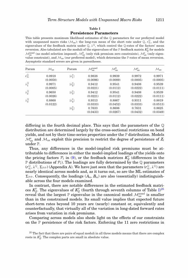
Table IPersistence Parameters
This table presents maximum likelihood estimates of the Q parameters for our preferred modelwith unspanned macro risks (Mus): the long-run mean of the short rate under Q, rQ
∞, and theeigenvalues of the feedback matrix under Q, λQ, which control the Q-rates of the factors’ meanreversion. Also tabulated are the moduli of the eigenvalues of the P feedback matrix KP
Z for modelsMnosel
us (no model selection imposed), M0us (only risk premium zero constraints), Me
us (only eigen-value constraint), and Mus (our preferred model), which determine the P-rates of mean reversion.Asymptotic standard errors are given in parentheses.
Param Mus Param Mnoselus M0
us Meus Mus
rQ∞ 0.0918 |λP
1 | 0.9838 0.9939 0.9972 0.9971(0.0058) (0.0096) (0.0089) (0.0005) (0.0005)
λQ
1 0.9971 |λP2 | 0.9412 0.9541 0.9408 0.9539
(0.0005) (0.0221) (0.0112) (0.0222) (0.0111)λ
Q
2 0.9650 |λP3 | 0.9412 0.9541 0.9408 0.9539
(0.0026) (0.0221) (0.0112) (0.0222) (0.0111)λ
Q
3 0.8868 |λP4 | 0.9313 0.8867 0.9311 0.8819
(0.0122) (0.0333) (0.0452) (0.0333) (0.0513)|λP
5 | 0.7633 0.8606 0.7631 0.8625(0.0433) (0.0267) (0.0432) (0.0349)
differing in the fourth decimal place. This says that the parameters of the Q
distribution are determined largely by the cross-sectional restrictions on bondyields, and not by their time-series properties under the P distribution. ModelsMe
us and Mus exploit this precision to restrict the degree of persistence of Ztunder P.
Thus, any differences in the model-implied risk premiums must be at-tributable to differences in either the model-implied loadings of the yields ontothe pricing factors Pt in (9), or the feedback matrices KP
Z (differences in theP distributions of Pt). The loadings are fully determined by the Q parameters(rQ
∞, λQ, �PP ) (Appendix A). We have just seen that the parameters (rQ∞, λQ) are
nearly identical across models and, as it turns out, so are the ML estimates of�PP . Consequently, the loadings (Am, Bm) are also (essentially) indistinguish-able across the four models examined.
In contrast, there are notable differences in the estimated feedback matri-ces KP
Z. The eigenvalues of KPZ (fourth through seventh columns of Table I)25
reveal that the largest P eigenvalue in the canonical model Mnoselus is smaller
than in the constrained models. Its small value implies that expected futureshort-term rates beyond 10 years are (nearly) constant or, equivalently andcounterfactually, that virtually all of the variation in long-dated forward ratesarises from variation in risk premiums.
Comparing across models also sheds light on the effects of our constraintson the P persistence of the risk factors. Enforcing the 11 zero restrictions in
25 The fact that there are pairs of equal moduli in all three models means that there are complexroots in KP
Z. The complex parts are small in absolute value.

1212 The Journal of Finance R©
Table IIRisk Premium Parameters
This table presents maximum likelihood estimates from our preferred model with unspanned macrorisks (Mus) of the parameters �0 and �1 governing expected excess returns on the PC-mimickingportfolios: xPC = �0 + �1 Zt. Standard errors are given in parentheses. Zeros correspond to the11 restrictions from our model selection.
P const PC1 PC2 PC3 GRO INF
PC1 0 −0.0896 −0.0510 0 0.1083 0.1729(0.0157) (0.0122) (0.0313) (0.0326)
PC2 0 0 0 −0.1035 −0.1487 0.0486(0.0330) (0.0307) (0.0123)
PC3 0 0 0 0 0 0
model M0us increases the largest eigenvalue of KP
Z from 0.984 to 0.994, andthus closes most of the gap between models Mnosel
us and Mus. In model M0us, Zt
is sufficiently persistent under P for long-dated forecasts of the short rate todisplay considerable time variation. A further increase in the largest eigenvalueof KP
Z comes from adding the eigenvalue constraint in model Mus.Estimates from model Mus of the parameters governing the expected excess
returns xPCjt ( j = 1, 2, 3) are displayed in Table II. The first and second rowsof �1 have nonzero entries, while the last row is set to zero by our modelselection criteria. It follows that exposures to PC1 and PC2 risks are priced,but exposure to PC3 risk is not priced, at the one-month horizon and duringour sample period. That both level and slope risks are priced, instead of justlevel risk as presumed by Cochrane and Piazzesi (2008), is one manifestation ofthe important influence of macro factors on risk premiums.26 The macro risksGRO and INF both have statistically significant effects on xPC1 and xPC2.In addition, xPC1 is influenced by PC1 and PC2, while xPC2 also depends onthe curvature factor PC3.
The signs of the coefficients imply that shocks to GRO induce pro- (counter-)cyclical movements in the risk premiums associated with exposures to PC1(PC2). These effects can be seen graphically in Figure 3 for models Mnosel
us andMus, where the shaded areas represent the NBER-designated recessions. Ex-posures to PC1 (PC2) lose money when rates fall (the curve flattens), whichis when investors holding long level (slope) positions make money. This ex-plains the predominantly negative (positive) expected excess returns on theannualized xPC1 (xPC2), and why it is small (large) during the 1990 and 2001recessions. There is broad agreement on the fitted excess returns across modelsMnosel
us and Mus.The premium on PC2 risk achieves its lowest value, and concurrently the
premium on PC1 risk achieves its highest value, during 2004 to 2005. BetweenJune 2004 and June 2006, the Federal Reserve increased its target federalfunds rate by 4% (from 1.25% to 5.25%). Yields on 10-year Treasuries actually
26 With a model fit to yields alone, Duffee (2010) also finds evidence for two priced risks.

Term Structure Models with Unspanned Macro Risks 1213
Figure 3. Excess returns. This figure depicts expected excess returns on the level- and slope-mimicking portfolios implied by our preferred model with unspanned macro risks, Mus, and thecounterpart without model selection applied, Mnosel
us .

1214 The Journal of Finance R©
Table IIIIntercept and Feedback Parameters
This table presents maximum likelihood estimates of KP0 and KP
Z for our preferred model withunspanned macro risks (Mus): EP
t [Zt+1] = KP0 + KP
ZZt. Standard errors are reported in parentheses.
KPZ
Z KP0 PC1 PC2 PC3 GRO INF
PC1 0.0002 0.9138 −0.0211 −0.0482 0.1083 0.1729(0.0000) (0.0156) (0.0121) (0.0031) (0.0313) (0.0326)
PC2 −0.0004 −0.0188 0.9697 0.0426 −0.1487 0.0486(0.0001) (0.0012) (0.0017) (0.0327) (0.0307) (0.0123)
PC3 0.0007 0.0155 0.0010 0.8757 0 0(0.0001) (0.0016) (0.0023) (0.0117)
GRO 0.0009 −0.0157 0.0191 −0.1035 0.8889 0.0233(0.0006) (0.0144) (0.0109) (0.0381) (0.0262) (0.0322)
INF 0.0003 −0.0002 0.0090 −0.0395 0.0347 0.9966(0.0002) (0.0086) (0.0056) (0.0223) (0.0161) (0.0194)
fell during this time, leading to a pronounced flattening of the yield curve, whichChairman Greenspan referred to as a conundrum. We revisit these patternsbelow.
ML estimates of KP0 and KP
Z governing the P drift of Zt are displayed inTable III for model Mus.27 The nonzero coefficients on (GROt−1, INFt−1) in therows for (PC1, PC2) are all statistically different from zero at conventionalsignificance levels, confirming that macro information is incrementally usefulfor forecasting future bond yields after conditioning on {PC1, PC2, PC3}.Additionally, the coefficients on the own lags of GRO and INF are largeand significantly different from zero, as expected given the high degree ofpersistence in these series.
For comparison, we also estimate a model Mspan that enforces spanning ofthe forecasts of output growth and expected inflation by the yield PCs. Re-call that this is the nested special case with the last two columns of KP
Z setto zero, as in (12). Similar models with macro spanning, based on the analy-ses of Bernanke, Reinhart, and Sack (2004) and Kim and Wright (2005), arereferenced by Chairman Bernanke in discussions of the impact of the macroe-conomy on bond risk premiums. For our choices of macro factors (GRO, INF),the χ2 statistic for testing the null hypothesis that the last two columns of KP
Zare zero is 1,189 (the 5% cutoff is 18.31). As we next show, the misspecifiedmodel Mspan implies very different term premiums from the model Mus withunspanned macro risks.
27 The zeros in row PC3 follow from the zero constraints on �1. A zero in �1 means that theassociated factor has the same effect on the P forecasts as Q forecasts (i.e., KQ
PP,i j = KPPP,i j ). Since,
by construction, the macro factors do not incrementally affect the Q expectations of the PCs, itfollows that Mt has no effect on the P forecasts of PC3.

Term Structure Models with Unspanned Macro Risks 1215
V. Forward Term Premiums
Excess holding period returns on portfolios of individual bonds reflect therisk premiums for every segment of the yield curve up to the maturity of theunderlying bond. A different perspective on market risk premiums comes frominspection of the forward term premiums, the differences between forwardrates for a q-period loan to be initiated in p periods, and the expected yieldon a q-period bond purchased p periods from now. Within affine MTSMs, bothforward rates and expected future q-year rates (and thus their difference) areaffine functions of the state Zt: FTPp,q
t = f p,q0 + f p,q
Z · Zt.To illustrate the differences between the risk premiums implied by MTSMs
with and without macro spanning, in Figure 1 we display three different vari-ants of the “in-two-for-one” forward term premium FTP2,1. One is the fittedpremium from our selected model Mus with unspanned macro risks. The pro-jection of this premium onto Pt is displayed as PMus. By construction, theMus premium depends on the entire set of risk factors Zt, and any differencesbetween Mus and PMus arise entirely from the effect of the unspanned com-ponents of Mt on FTP2,1
t . The Mus premium shows pronounced countercyclicalswings about a gently downward-drifting level. The differences between theMus and PMus premiums induced by unspanned macro risks are largest dur-ing the late 1980s and the conundrum period, as well as at most peaks andtroughs of FTP2,1. These peak-trough differences are a consequence in largepart of the dependence of the Mus premium on GRO.
Equally striking from Figure 1 are the very different patterns in the fittedFTP2,1 from model Mus and the premium from model Mspan that constrainsEt−1[Mt] to be spanned by Pt−1 (as in (12)). Both PMus and Mspan are graphsof premiums that are spanned by Pt. However, they will coincide only when themacro-spanning constraint imposed in model Mspan is consistent with the data-generating process for Zt. In fact, the cyclical turning points of the premiumsfrom models Mus and Mspan are far from synchronized: Mspan drifts muchlower during the late 1990s, and it stays (relatively) high after the burst ofthe dot-com bubble when Mus was declining along with the Federal Reserve’starget federal funds rate. Clearly, the macro-spanning constraint distorts thefitted risk premiums in economically significant ways.
Turning to longer-dated forward term premiums, the standardized “in-nine-for-one” premium FTP9,1 is displayed in Figure 4, along with a standardizedversion of GRO. The band about the fitted FTP9,1 is the 95% confidence bandbased on the precision of the ML estimates of f 9,1
Z . Importantly, with condi-tioning on both the macro factors and the shape of the yield curve, the im-plied FTP9,1 does not follow an unambiguously countercyclical pattern. WhileFTP9,1 is high during the recession of the early 1990s, there are subperi-ods during 1993 through 2000 when GRO and FTP9,1 track each other quiteclosely.
The sources of this procyclicality are revealed by the estimated coefficientsf p,1Z that link the FTPs to Zt (Table IV). The negative weights on GRO and
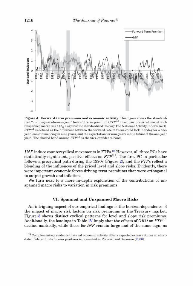
1216 The Journal of Finance R©
Figure 4. Forward term premnum and economic activity. This figure shows the standard-ized “in-nine-years-for-one-year” forward term premium (FTP9,1) from our preferred model withunspanned macro risk (Mus), against the standardized Chicago Fed National Activity Index (GRO).FTP9,1 is defined as the difference between the forward rate that one could lock in today for a one-year loan commencing in nine years, and the expectation for nine years in the future of the one-yearyield. The shaded band around FTP9,1 is the 95% confidence band.
INF induce countercyclical movements in FTPs.28 However, all three PCs havestatistically significant, positive effects on FTP9,1. The first PC in particularfollows a procyclical path during the 1990s (Figure 2), and the FTPs reflect ablending of the influences of the priced level and slope risks. Evidently, therewere important economic forces driving term premiums that were orthogonalto output growth and inflation.
We turn next to a more in-depth exploration of the contributions of un-spanned macro risks to variation in risk premiums.
VI. Spanned and Unspanned Macro Risks
An intriguing aspect of our empirical findings is the horizon-dependence ofthe impact of macro risk factors on risk premiums in the Treasury market.Figure 3 shows distinct cyclical patterns for level and slope risk premiums.Additionally, the loadings in Table IV imply that the effects of GRO on FTPp,1
decline markedly, while those for INF remain large and of the same sign, as
28 Complementary evidence that real economic activity affects expected excess returns on short-dated federal funds futures positions is presented in Piazzesi and Swanson (2008).

Term Structure Models with Unspanned Macro Risks 1217
Table IVForward Term Premium Parameters
This table presents coefficients f p,10 and f p,1
Z determining the mapping between the forward term
premiums FTPp,1t and the state Zt in our preferred model with unspanned macro risks (Mus):
FT P p,1t = f p,1
0 + f p,1Z · Zt. FTPp,1 is defined as the difference between the forward rate that one
could lock in today for a one-year loan commencing in p years and the expectation for p years inthe future of the one-year yield. Standard errors are reported in parentheses.
const PC1 PC2 PC3 GRO INF
2-for-1 −0.0153 1.1522 0.2227 0.9066 −0.5950 −1.5141(0.0108) (0.1987) (0.1841) (0.3768) (0.2786) (0.4280)
5-for-1 −0.0103 0.9090 0.4179 0.4262 0.2430 −0.8301(0.0137) (0.1166) (0.1238) (0.2641) (0.1737) (0.3989)
9-for-1 −0.0023 0.7392 0.5341 0.6875 0.0828 −0.7623(0.0151) (0.0813) (0.0983) (0.1600) (0.1046) (0.2994)
the contract horizon p increases. To what extent are the cyclical risk profiles ofTreasury bonds determined by shocks to unspanned versus spanned macroe-conomic factors?
Analogous to the loadings on GRO in Table IV, we find that a positive inno-vation to GRO tends to lower FTP1,1, while (as the table shows) being largelyneutral for FTP9,1, thus inducing a steepening of the forward premium curve(increase in SLF9
1 ≡ FTP9,1 − FTP1,1). The impulse responses (IRs) of SLF91 to
innovations in spanned (SGRO) and unspanned (OGRO) output growth aredisplayed in the left panel of Figure 5 for model Mus.29 A shock to OGROinduces an immediate, large steepening of the forward premium curve, and itseffect then dissipates rapidly over the following year. This dominant role forOGRO emerges even though SGRO is ordered first in the underlying VAR.The macro-spanning restriction rules out any effect of OGRO on SLF9
1 .Moreover, macro-spanning restrictions severely distort the responses of
SLF91 to shocks to total output growth GRO. The response of SLF9
1 to a GROshock in model Mus (right panel of Figure 5) looks nearly identical to its re-sponse to OGRO in the adjacent figure, a manifestation of the large unspannedcomponent of GRO. On the other hand, under macro spanning in model Mspan,the response of SLF9
1 to a growth shock is (virtually) zero at all horizons.Evidently, shutting down the feedback from GRO to future Z drives out theeconomically important effects of growth on the slope of the forward premiumcurve.
In comparison to GRO, survey expectations of inflation are largely spannedby Pt (85% of its variation) and INF shows higher persistence. The latterproperty of INF gives it a level-like effect in that innovations in INF (roughly
29 These IRs are computed from the (ordered) VAR of (SGRO, SINF, OGRO, OINF, SLF91 )
implied by model Mus, where SGRO is the model-implied projection of GROt onto the PCs Pt andOGROt is the residual from this projection.

1218 The Journal of Finance R©
-10
-5
0
5
10
15
20
12010896847260483624120
Resp
onse
(bps
)
Time (months)
SGRO
OGRO
-10
-5
0
5
10
15
20
12010896847260483624120
Resp
onse
(bps
)
Time (months)
CM0E
Kim-Wri
M← us
M← span
Figure 5. Response to growth shock. The left panel plots the impulse responses of the slopeof the forward premium curve, SLF9
1 = FTP9,1 − FTP1,1, to shocks to either (SGRO, OGRO) fromour preferred model with unspanned macro risks (Mus). The right panel compares the responsesof SLF9
1 to innovations in total GRO across our preferred model with unspanned macro risks(Mus) and the nested model that enforces spanning of expectations of the macro variables by theyield PCs (Mspan). SGRO, spanned growth, is the projection of GRO onto the PCs; OGRO is thecomponent of GRO orthogonal to the PCs. FTPp,1 is defined as the difference between the forwardrate that one could lock in today for a one-year loan commencing in p years and the expectationfor p years in the future of the one-year yield.
-20
-15
-10
-5
0
5
10
15
20
25
30
12010896847260483624120Resp
onse
(bps
)
Time (months)
SINF
OINF
-10
-5
0
5
10
15
20
25
12010896847260483624120
Resp
onse
(bps
)
Time (months)
SINF
OINF
Figure 6. Response to inflation shock. Each panel plots the impulse responses of forwardterm premiums (FTPs) to shocks to spanned and unspanned inflation (SINF, OINF), implied byour preferred model with unspanned macro risks (Mus). SINF is the projection of INF onto thePCs; OINF is the component of INF orthogonal to the PCs. FTPp,1 is defined as the differencebetween the forward rate that one could lock in today for a one-year loan commencing in p yearsand the expectation for p years in the future of the one-year yield.
uniformly) affect the entire maturity spectrum of yields. While the formerproperty might lead one to presume that shocks to unspanned inflation (OINF)have inconsequential effects on risk premiums, this is not the case. Theseproperties of inflation risk can be seen from the IRs of FTPp,1
t , p = 2, 9, toshocks to OINF and SINF displayed in Figure 6. The effects of OINF persistfor several years, owing to the near-cointegration of INF with the priced riskfactors (PC1, PC2).

Term Structure Models with Unspanned Macro Risks 1219
There is also near-symmetry in the effects of (SINF, OINF) on forward termpremiums. Initially, unspanned inflation shocks lead to lower FTPs, but theeffects turn positive within a year. Innovations in SINF, in contrast, havelarge positive impact effects on FTPs that dissipate slowly over a couple ofyears. The dominant effect on FTP9,1 at long horizons comes from unspannedinflation risk.
Returning to the period of the conundrum during 2004 to 2005, notice fromFigure 4 that this was a period when GRO was increasing and long-dated for-ward term premiums were falling. In speaking about the conundrum, Chair-man Bernanke asserted that “a substantial portion of the decline in distant-horizon forward rates of recent quarters can be attributed to a drop in termpremiums. . . . the decline in the premium since June 2004 appears to havebeen associated mainly with a drop in the compensation for bearing real in-terest rate risk.”30 According to our model, the forward term premium FTP9,1
indeed declined by 112 basis points between June 2004 and June 2005,31 butby June 2006 had retracted to almost exactly its June 2004 level.
As to whether these patterns reflect changing premiums on real interestrate risk, of the initial decline about 30 basis points can be attributed to or-thogonal inflation and almost none to orthogonal growth, with the remainderaccounted for by factors spanned by yields. Complementary to this, we findthat the expected excess return on a bond portfolio mimicking the negative ofspanned inflation—an indicator of the compensation required by investors fac-ing spanned inflation risk—fell by roughly 60 basis points between June 2004and June 2005. Both findings are indicative of a potentially more significantrole played by inflation risks during the conundrum period than suggested byChairman Bernanke.
Symmetric to this discussion is the interesting question of how changes interm premiums affect real economic activity. Bernanke, in his 2006 speech,argues that a higher term premium will depress the portion of spending thatdepends on long-term interest rates and thereby have a dampening economicimpact. In linearized New Keynesian models in which output is determined bya forward-looking IS equation (such as the model of Bekaert, Cho, and Moreno(2010)), current output depends only on the expectation of future short rates,leaving no role for a term premium effect. Time-varying term premiums doarise in models that are linearized at least to the third order (e.g., Ravennaand Seppala (2008)). We examine the response of real economic activity andinflation expectations to innovations in FTPp,1 (p = 2, 9) in the context of modelMus.32
Initially, a one-standard-deviation increase in FTP2,1 has a small negativeimpact on OGRO over a period of about 18 months, and has virtually no ef-fect on SGRO (left panel of Figure 7). Shocks to the long-term premium FTP9,1
30 See his speech before the Economic Club of New York on March 20, 2006 titled “Reflectionson the Yield Curve and Monetary Policy.”
31 The model also shows an even larger decline of 175 basis points between July 2003 and June2005.
32 The ordering of the model-implied VAR is (FTPp,1, SGRO, SINF, OGRO, OINF).

1220 The Journal of Finance R©
-4
-3
-2
-1
0
1
2
12010896847260483624120
Resp
onse
(bps
)
Time (months)
SGRO
OGRO
-1
0
1
2
3
4
12010896847260483624120
Resp
onse
(bps
)
Time (months)
SGRO
OGRO
Figure 7. Response to term premium shock. Each panel plots the impulse responses ofspanned and unspanned growth (SGRO, OGRO) to shocks in forward term premiums (FTPs)implied by our preferred model with unspanned macro risks (Mus). SGRO is the projection ofGRO onto the yield PCs; OGRO is the component of GRO orthogonal to the PCs. FTPp,1 is de-fined as the difference between the forward rate that one could lock in today for a one-year loancommencing in p years and the expectation for p years in the future of the one-year yield.
induce a short-lived positive effect on unspanned GRO (right panel of Figure 7).Again the premium shock has no effect on SGRO.33 These responses presenta more differentiated perspective on the economic linkages set forth by Chair-man Bernanke. A negative impact on economic activity arises from short- tomedium-term risk premiums, not long-dated premiums. Moreover, the effectsare virtually entirely through unspanned real economic activity, a componentof growth that is absent from the models he cites in his analysis.
VII. Extended Sample Analysis
In estimating our macro term structure models, we face a tradeoff betweenthe potential small-sample bias arising from our selected sample period andbiases that would arise from nonstationarity owing to structural breaks in alonger sample. The existing literature is divided on how this tradeoff is bestresolved.34 Based on extant research, we argue in Section I that our sampleperiod (1985 to 2007) is the longest recent sample that can reasonably be clas-sified as a single regime (free from structural breaks). Small-sample concernsare mitigated somewhat by sampling at a monthly frequency, and by exploit-ing information about persistence from the pricing distribution. Though we
33 The absence of effects on SGRO is consistent with the results in Ang, Piazzesi, and Wei(2006) that term premiums are insignificant in predicting future GDP growth within an MTSMthat enforces spanning of GDP growth by bond yields. What their model does not accommodate isour finding that term premium shocks do affect growth through their effects on unspanned realactivity.
34 Ang and Piazzesi (2003) and Ang, Dong, and Piazzesi (2007) use relatively long postwarsamples starting in the early 1950s. Bikbov and Chernov (2010) start their sample in 1970 underthe caveat of structural stability concerns. Smith and Taylor (2009) cite evidence of a structuralbreak in the early 1980s and consequently proceed with a split-sample analysis around that breakpoint.

Term Structure Models with Unspanned Macro Risks 1221
document an economically important link between yields and unspanned macrorisks, such links may well be different in different time periods. Indeed, it isour prior that unspanned macro risks are qualitatively important across policyregimes, but likely in quantitatively different ways.
A. Regime-Switching Model
To explore this conjecture jointly with our assumption that the post-1985 pe-riod is adequately treated as a single regime, we estimate a regime-switchingversion of our model, adapting the methodology of Dai, Singleton, and Yang(2007). Our extended sample starts in November 1971 (the earliest date withconsistent availability of 10-year yield data, as discussed, for example, inGurkanyak, Sack, and Wright (2007)) and ends in December 2007. We usethe same cross section of yields, and the same macroeconomic growth indica-tor (the Chicago Fed National Activity Index) as before, but we can no longeruse Blue Chip inflation forecasts, as these are not available prior to the early1980s. Instead, we define INF as the 12-month moving average of core CPIinflation, a measure that is highly correlated (> 90%) with Blue Chip inflationforecasts over the period for which both inflation measures are available. Weallow for two regimes with time-homogeneous transition matrices πP and πQ.All parameters except λQ are permitted to depend on the current regime (themaximally flexible regime-switching specification under which bond prices re-main exponential-affine). We do not otherwise constrain parameters or performa model selection procedure as in Section IV.
Figure 8 shows that the maximum-likelihood-based regime classification35 isindicative of a structural break in our data occurring in the mid-1980s, broadlyconsistent with the consensus in the literature. To a first approximation, thesample is divided into an early (pre-1985) and late (post-1985) regime. In partic-ular, with the exception of the first year and three isolated months, the sampleperiod we use in our main analysis is contained within a single regime. Con-versely, the pre-1985 period is predominantly classified as a different regime.This finding supports our claim that the 1985 to 2007 period is adequatelytreated as a single regime, while this would not be the case for a longer sample.
The two regimes differ in economically meaningful ways, and consistentwith the findings in previous research. In regime 2 (the “late” regime), thelong-term mean of the short rate under the risk-neutral measure is lower,the system of yields and macro variables is more persistent and has lowerconditional volatility (reflecting the “Great Moderation” analyzed by Stock andWatson (2002)), and the regime is more stable. While GRO affects level andslope risk premiums comparably across regimes, not surprisingly, given thehigh inflation in the first regime, INF has a much larger effect on level risk inregime 1 than regime 2 (for exact parameter estimates, see Appendix F). These
35 As is standard, we classify an observation as belonging to the regime with the highest ex post(smoothed) probability.

1222 The Journal of Finance R©
Figure 8. Regime classification. This figure shows the regime classification from a two-regimemodel with unspanned macro risks. The hatched area represents the first regime, while shadedareas indicate NBER recession periods.
differentiated results would be obscured if we estimated a single-regime modelover the longer sample period.
B. Out-of-Sample Analysis
Also of interest are the properties of our model’s implied risk premiumsduring the post-2007 crisis period. Up to this point we have excluded thisperiod due to concerns not only about another structure break, but also aboutthe ability of a Gaussian term structure model to adequately capture yielddynamics near the zero lower bound. With this cautionary observation inmind, we briefly examine the out-of-sample differences between our preferredmodel with unspanned macro variables, Mus, and the alternative modelwith spanned macro factors, Mspan. For this purpose, we compute fittedrisk premiums (based on model estimates for the 1985 to 2007 sample)starting from the end of our estimation sample and continuing throughJuly 2012.
Figure 9 plots the in-two-for-one forward term premiums implied by mod-els Mus and Mspan. As we discuss in Section V, these forward term premi-ums bear limited resemblance in sample. Out of sample, the differences areeven more pronounced, particularly in the 2008 to 2010 period. The term pre-mium implied by model Mus initially increases sharply in 2008 with a rapidly

Term Structure Models with Unspanned Macro Risks 1223
Figure 9. Out-of-sample forward term premiums. This figure depicts out-of-sample forwardterm premiums FTP2,1 for our preferred model with unspanned macro risks (Mus), and the nestedmodel that enforces spanning of expectations of the macro variables by the yield PCs (Mspan).FTP2,1 is defined as the difference between the forward rate that one could lock in today for aone-year loan commencing in two years and the expectation for two years in the future of theone-year yield.
deteriorating economic outlook. It rebounds later that year, and declines by asimilar magnitude in late 2010 to early 2011. The declines roughly coincidewith the Federal Reserve’s first two quantitative easing programs (QE1 andQE2), a stated objective of which was to lower forward term premiums. Themovements in the Mspan-implied forward term premium are much more sub-dued, and harder to reconcile with economic events. For instance, the forwardterm premium increases around QE1.
VIII. Elaborations and Extensions
Our framework can be applied in any Gaussian pricing setting in which se-curity prices or yields are affine functions of a set of pricing factors Pt andrisk premiums depend on a richer set of state variables that have predictivepower for Pt under the physical measure P. Accordingly, it is well suited toaddressing a variety of economic questions about risk premiums in bond andcurrency markets, as well as in equity markets when the latter pricing prob-lems map into an affine pricing model (e.g., Bansal, Kiku, and Yaron (2012b)).Though neither the state variables nor the pricing factors exhibit time-varyingvolatility in the settings examined in this paper, our basic framework andits computational advantages are likely to extend to affine models with time-varying volatility. Incorporating time-varying volatility would allow for the

1224 The Journal of Finance R©
possibility of volatility factors that are unspanned by bond prices or macrovariables, thereby generalizing Collin-Dufresne and Goldstein (2002). As inour setting, such unspanned volatility factors may also drive expected returns(as in Joslin (2013b)). Exploration of this extension is deferred to future re-search.
A distinct, though complementary, question is: what are the structural eco-nomic underpinnings of the substantial effects of unspanned macro variableson risk premiums that we document in our empirical analysis? At this junc-ture, we comment briefly on the insights that our reduced-form model revealsabout the nature of risk premiums in the U.S. Treasury market, again leav-ing the task of developing a structural model with these features to futureresearch.
Many of the extant structural models of term premiums in bond marketsrule out by construction any link between unspanned macro risks and termpremiums. This is trivially the case in the model of Bekaert, Cho, and Moreno(2010), because they assume constant risk premiums. Gallmeyer et al. (2007)add preferences with habit shocks (as in Abel (1990)) to a policy rule to obtaina setting with time-varying risk premiums. However, their models also implythat real economic activity (in their case consumption growth) and inflation arefully spanned by the current yield curve. Indeed, all of the equilibrium modelsof bond yields that fall within the family of affine pricing models that we areaware of implicitly impose macro-spanning conditions (see Le and Singleton(2013)).
We can imagine how unspanned macro risks could arise through additionalconstraints on agents’ preferences, policy rules, and exogenous sources of un-certainty. For instance, in a model with preferences of the habit type, if theshort rate is affine in growth and one component of growth has the same mean-reversion as the habit variable (for example, as growth decreases, risk aversionincreases according to such a rule), then there may be unspanned growth risk.Within an affine pricing setting, such unspanned growth could be allowed toimpact policy rules and the inflation process. Whether this avenue for accom-modating unspanned risks is fruitful is ultimately a quantitative question thatwarrants further exploration. A primary take-away from our findings is thatthis or some other complementary economic mechanism seems needed to ra-tionalize our core empirical findings.
Our findings also speak to the policy conclusions drawn from struc-tural models. A standard framework for policy analysis within a struc-tural term structure model is the New Keynesian model, as in Clar-ida, Gali, and Gertler (1999). For example, Gallmeyer, Hollifield, and Zin(2005) and Gallmeyer et al. (2007) examine affine term structure modelsthat embed Taylor- or McCallum-style monetary policy rules and (implic-itly) enforce spanning of all macro variables by bond yields. Our resultssuggest that a monetary authority may affect the output gap and infla-tion through channels that leave bond yields unaffected, by having a si-multaneous effect on expectations about the future short rates and riskpremiums.

Term Structure Models with Unspanned Macro Risks 1225
IX. Conclusion
This paper explores the effects of unspanned macro risks on risk premiumsin bond markets. We find that shocks to unspanned real economic activity andinflation have large effects on term premiums in U.S. Treasury markets and,symmetrically, shocks to forward term premiums have substantial effects onreal economic activity primarily through their effects on unspanned real outputgrowth. Moreover, we document an important role for unspanned inflation risksin shaping term premiums, despite the fact that a large portion of the variationin inflation is spanned by bonds.
To assess the role of unspanned macro risks, we develop a canonicalarbitrage-free Gaussian MTSM in which the state vector includes macroe-conomic variables that are not perfectly spanned by contemporaneous bondyields, and in which these macro variables can have significant predictive con-tent for excess returns on bonds over and above the information in bond yields.We show that this canonical representation of the model lends itself to easyinterpretation and attains the global maximum of the likelihood function es-sentially instantaneously.
Properties of the fitted historical distributions of bonds and pricing factors inour MTSM are very different from what is implied by both a factor-VAR modelor an unconstrained version of our canonical model. Owing to the constraintssuggested by our model selection criteria, the persistence properties of bondyields, and hence the relative importance of expected future spot rates versusforward term premiums, are very different in our preferred model compared toits unconstrained counterpart. This suggests that, when estimating MTSMs,one should undertake similar model selection exercises to systematically reducethe dimension of the parameter space, as this might similarly mitigate small-sample bias problems.
Our findings raise several intriguing questions for future research. Un-spanned macro risks, particularly real economic risks, have large effects on for-ward term premiums over short- to intermediate-term horizons. What are theeconomic sources of these unspanned risks? On the other hand, a substantialportion of the variation in long-dated forward term premiums is attributableto economic factors that are orthogonal to both spanned and unspanned outputand inflation. What is the nature of these macro risks that are so important inTreasury markets and yet are orthogonal to output growth and inflation? Sincethe onset of the financial crisis, there has been considerable discussion aboutthe roles of global imbalances and disruptions in the financial intermediationsectors. Our modeling framework provides a means to systematically examinethese possibilities within arbitrage-free dynamic term structure models.
Initial submission: October 7, 2010; Final version received: October 20, 2013Editor: Campbell Harvey

1226 The Journal of Finance R©
Appendix A: Bond Pricing in GDTMs
The price of an m-month zero-coupon bond is given by
Dt,m = EQt[e− ∑m−1
i=0 rt+i] = eAm+Bm·Pt , (A1)
where (Am,Bm) solve the first-order difference equations
Am+1 − Am = (KQ
0
)′Bm + 12B′
m�PPBm − ρ0 (A2)
Bm+1 − Bm = (KQ
1
)′Bm − ρ1 (A3)
subject to the initial conditions A0 = 0,B0 = 0. See, for example, Dai and Sin-gleton (2003). The loadings for the corresponding bond yield are Am = −Am/mand Bm = −Bm/m.
Appendix B: Conditions for Unspanned Risks
In this appendix, we derive the nominal pricing kernel (equivalently, risk-neutral distribution of the N risk factors Zt) in order to have a model withunspanned macro risks. We begin with the general specification of the nominalpricing kernel in (1) with short rate given in (3) and dynamics of the statevariable Zt given by (2). Macro variables are added to the system through
Mt = γ0Z + γ1Z · Zt. (B1)
Notice that this specification is the most general affine Gaussian model. Inparticular, it subsumes the case in which some elements of Zt are themselvesmacro variables by assuming that rows of γ1Z are standard basis vectors (withcorresponding entries in γ0Z set to zero).
From the pricing kernel, we derive the risk-neutral distribution of Zt through
dQ
dP
∣∣∣∣∣t
= e− ∑ts=1
[12 �′
Z,s�Z,s−�′Z,sη
Ps
].
Our assumption is that the market prices of risk are affine so that, followingthe notation of Section IV, we have
�Z,t = �−1/2ZZ (�0 + �1 Zt)
and the risk-neutral distribution is given by
Zt = KQ
0Z + KQ
1ZZt−1 +√
�ZηPt ηP
t ∼ N(0, I). (B2)
Here (KQ
0Z, KQ
1Z) are given through the market prices of risk:
KQ
0Z = KP0Z − �0, (B3)
KQ
1Z = KP1Z − �1. (B4)

Term Structure Models with Unspanned Macro Risks 1227
Following Joslin (2013a), we see that the macro risks are unspanned macrorisks if there are (N − R) vectors {v1, v2, . . . , vN−R} so that for each i:
(1) vi · ρ1Z = 0.(2) v′
i KQ
1Z is a multiple of KQ
1Z (i.e., vi is a left eigenvector of KQ
1Z).(3) γ1 · vi = 0.
The first condition ensures that the factor vi · Zt does not affect the shortrate while the second condition ensures that vi · Zt does not affect risk-neutralexpectations of the short rate (for any horizon). The final condition ensuresthat the factor vi · Zt has an effect on the macro variables. We can relax thiscondition so that, if vi · Zt = 0, there can be a factor that is not identified by thejoint cross section of bond prices and Mt.
Notice that the conditions above are all specified directly in terms of therisk-neutral parameters. Alternatively, one could use (B3) and (B4) to expressthe conditions for unspanned macro risk in terms of the market prices of riskand P parameters.
Appendix C: A Canonical Model with Unspanned Macro Risks
In this section, we prove that our form of MTSM with unspanned macrorisks is canonical in the following sense. Consider the family of MTSMs withnominal pricing kernel given in (1), with short rate given in (3), with dynamicsof the state variable Zt given by (2), and with macro variables given in (B1). ForZt of dimension N and Mt of dimension R, we denote UMAR
0 (N) to be this familywhen the macro risks are unspanned. To prove that our family is canonical, weshow that every such MTSM is observationally equivalent (given data on themacro variables and the cross section of all yields) to exactly one model withthe specification given in Section II.
To prove the existence of such a representation, we begin with a genericmodel with a latent Zt driving yields and macro factors and apply the affinerotations as in Dai and Singleton (2000). Taking the loadings from (9) we maywrite [
Pt
Mt
]=
[W A
γ0
]+
[W B
γ1
]Zt, (C1)
where W are the weights in the principal components and (A, B) are the stackedloadings for the corresponding maturities. The matrix [WB; γ1] is invertible bythe spanning assumptions in the previous section. Thus, after we apply theaffine transformation of (C1) to our parameters, we obtain a model with (Pt, Mt)as the state variable. The spanning assumptions in the previous section showthat Pt is Q Markov and that the short rate must depend only on Pt (and notMt). The results of Joslin, Singleton, and Zhu (2011) then allow us to uniquelyparameterize the Q-distribution of Pt through (�PP , λQ, rQ
∞). The Q-distributionof Mt is not identified in our specification without further data. In the presenceof securities with payoffs directly tied to Mt, the risk-neutral dynamics could

1228 The Journal of Finance R©
be fully specified (equivalently, the entire pricing kernel rather than just theprojection onto bond returns could be identified).
Appendix D: Returns on Generalized Mimicking Portfolios
Consider a collection of N yields, {yn1t , . . . , ynN
t }, and a given linear combina-tion ya
t = ∑Ni=1 ai y
nit of these yields (ya
t could be a principal component, or theprojection of a macro variable onto the yields). Our first goal is to find weights{wi}N
i=1 such that value Pwt = ∑N
i=1 wi Pnit of a portfolio of zero-coupon bonds
locally tracks changes in yat ; that is,
dPwt
dyat
=N∑
i=1
dPwt
dynit
dynit
dyat
= 1. (D1)
Since, by definition, Pnit = exp(−ni y
nit ), we have dPni
t /dynit = −ni Pni
t . Therefore,(D1) can be rewritten as
−N∑
i=1
wini Pnit
1ai
= 1,
which will hold for weights
wi = − ai
Nni Pnit
.
Next, consider the one-period excess return on portfolio Pwt :
∑i
wi(Pni−1
t+1 − ert Pnit
)∣∣∣∑
i
wi Pnit
∣∣∣ =−
∑i
ai/ni(Pni−1
t+1
/Pni
t − ert)
∣∣∣ ∑i
ai/ni
∣∣∣ .
This is a weighted average of the returns on the individual zero-coupon bonds.Now, it follows from Le, Singleton, and Dai (2010) that Pni
t = exp(−Ani − BniPt),and further that
EP[Pni−1
t+1 /Pnit
] = exp{Bni−1
[(KQ
0 − KP0
) + (KQ
P − KPP)Zt
] + rt}.
Therefore, to a first-order approximation, the expected excess return on port-folio Pw
t is given by
∑i
ai/ni Bni−1[(
KP0 − KQ
0
) + (KPP − KQ
P )Zt]
∣∣∣∑i
ai/ni
∣∣∣ .

Term Structure Models with Unspanned Macro Risks 1229
Since we rotate our model such that the first R elements of Zt correspond tothe first R principal components of yields, and since by definition
PCjt =N∑
i=1
�ji yni
t =N∑
i=1
�ji (Ani /ni + Bni /niPt),
it follows that∑
i �ji Bni /ni is the selection vector for the jth element, j ∈
{1, . . . , R}. Thus, under the further approximation that Bni−1 ≈ Bni , the ex-pected excess return on the portfolio mimicking PCj, xPCj, is given by the jth
row of (KP
0 − KQ
0
) + (KPP − KQ
P)Zt
scaled by |∑i �ji /ni|. While an approximation for the one-period expected excess
return in discrete time, this relationship is exact for the instantaneous expectedexcess return in the continuous-time limit.
Appendix E: Details on Model Selection
As discussed in Section IV.A, we select among a total of 219 model specifica-tions distinguished by different sets of restrictions on the market price of riskparameters, and the maximum eigenvalue of KP
Z. In estimating the baseline(unrestricted) version of our model, we reduce the computational burden by
Figure E1. Model selection. Each of the 219 model specifications we consider corresponds toa point on the graph. The likelihood frontiers “Without EV” and “With EV” trace out the modelswith the highest likelihood for a given number of restrictions, without and with the maximumeigenvalue constraint on the feedback matrix KP
Z imposed. The straight lines are “indifferencecurves” for each of the three information criteria, Akaike (1973, AIC), Hannan and Quinn (1979,HQIC), and the Bayesian criterion proposed by Schwarz (1978, SBIC). The marked tangency pointscorrespond to the models selected under each criterion.
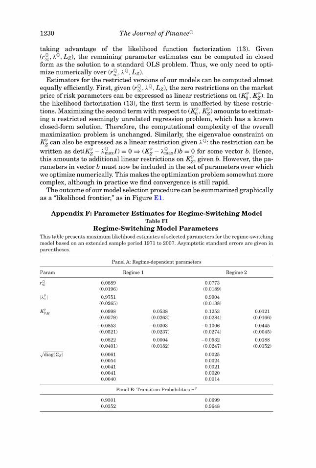
1230 The Journal of Finance R©
taking advantage of the likelihood function factorization (13). Given(rQ
∞, λQ, LZ), the remaining parameter estimates can be computed in closedform as the solution to a standard OLS problem. Thus, we only need to opti-mize numerically over (rQ
∞, λQ, LZ).Estimators for the restricted versions of our models can be computed almost
equally efficiently. First, given (rQ∞, λQ, LZ), the zero restrictions on the market
price of risk parameters can be expressed as linear restrictions on (KP0 , KP
Z). Inthe likelihood factorization (13), the first term is unaffected by these restric-tions. Maximizing the second term with respect to (KP
0 , KPZ) amounts to estimat-
ing a restricted seemingly unrelated regression problem, which has a knownclosed-form solution. Therefore, the computational complexity of the overallmaximization problem is unchanged. Similarly, the eigenvalue constraint onKP
Z can also be expressed as a linear restriction given λQ: the restriction can bewritten as det(KP
Z − λQmax I) = 0 ⇒ (KP
Z − λQmax I)b = 0 for some vector b. Hence,
this amounts to additional linear restrictions on KPZ, given b. However, the pa-
rameters in vector b must now be included in the set of parameters over whichwe optimize numerically. This makes the optimization problem somewhat morecomplex, although in practice we find convergence is still rapid.
The outcome of our model selection procedure can be summarized graphicallyas a “likelihood frontier,” as in Figure E1.
Appendix F: Parameter Estimates for Regime-Switching ModelTable FI
Regime-Switching Model ParametersThis table presents maximum likelihood estimates of selected parameters for the regime-switchingmodel based on an extended sample period 1971 to 2007. Asymptotic standard errors are given inparentheses.
Panel A: Regime-dependent parameters
Param Regime 1 Regime 2
rQ∞ 0.0889 0.0773
(0.0196) (0.0189)
|λP1 | 0.9751 0.9904
(0.0265) (0.0138)
KPPM 0.0998 0.0538 0.1253 0.0121
(0.0579) (0.0263) (0.0284) (0.0166)
−0.0853 −0.0303 −0.1006 0.0445(0.0521) (0.0237) (0.0274) (0.0045)
0.0822 0.0004 −0.0532 0.0188(0.0401) (0.0182) (0.0247) (0.0152)√
diag(�Z) 0.0061 0.00250.0054 0.00240.0041 0.00210.0041 0.00200.0040 0.0014
Panel B: Transition Probabilities πP
0.9301 0.06990.0352 0.9648
Term Structure Models with Unspanned Macro Risks 1231
REFERENCES
Abel, Andrew, 1990, Asset prices under habit formation and catching up with the Joneses, AmericanEconomic Review Papers and Proceedings 80, 38–42.
Akaike, Hirotugu, 1973, Information theory and an extension of the likelihood principle, in BorisPetrov and Frigyes Csaki, eds.: Proceedings of the Second International Symposium of Infor-mation Theory (Akademiai Kiado, Budapest).
Ang, Andrew, Sen Dong, and Monika Piazzesi, 2007, No-arbitrage Taylor rules, Working paper,Columbia University.
Ang, Andrew, and Monika Piazzesi, 2003, A no-arbitrage vector autoregression of term structuredynamics with macroeconomic and latent variables, Journal of Monetary Economics 50, 745–787.
Ang, Andrew, Monika Piazzesi, and M. Wei, 2006, What does the yield curve tell us about GDPgrowth?, Journal of Econometrics 131, 359–403.
Bansal, Ravi, Dana Kiku, and Amir Yaron, 2012a, An empirical evaluation of the long-run risksmodel for asset prices, Critical Finance Review 1, 183–221.
Bansal, Ravi, Dana Kiku, and Amir Yaron, 2012b, Risks for the long run: Estimation with timeaggregation, Working paper, Duke University.
Bansal, Ravi, and Ivan Shaliastovich, 2013, A long-run risks explanation of predictability puzzlesin bond and currency markets, Review of Financial Studies 1, 1–33.
Barillas, Francisco, 2011, Can we exploit predictability in bond markets?, Working paper, EmoryUniversity.
Bauer, Michael, 2011, Bayesian estimation of dynamic term structure models under restrictionson risk pricing, Working paper, Federal Reserve Bank of San Francisco.
Bauer, Michael, Glenn Rudebusch, and Jing Wu, 2012, Correcting estimation bias in dynamic termstructure models, Journal of Business & Economic Statistics 30, 454–467.
Bekaert, Geert, Seonghoon Cho, and Antonio Moreno, 2010, New Keynesian macroeconomics andthe term structure, Journal of Money, Credit, and Banking 42, 33–62.
Bernanke, Ben, Vincent Reinhart, and Brian Sack, 2004, Monetary policy alternatives and thezero bound: An empirical assessment, Brookings Papers on Economic Activity 2, 1–100.
Bikbov, Ruslan, and Mikhail Chernov, 2010, No-arbitrage macroeconomic determinants of theyield curve, Journal of Econometrics 159, 166–182.
Campbell, John, Adi Sunderam, and Luis Viceira, 2013, Inflation bets or deflation hedges? Thechanging risks of nominal bonds, Working paper, Harvard University.
Chernov, Mikhail, and Philippe Mueller, 2012, The term structure of inflation expectations, Jour-nal of Financial Economics 106, 367–394.
Cieslak, Anna, and Pavol Povala, 2013, Expected returns in Treasury bonds, Working paper,Northwestern University.
Clarida, Richard, Jordi Galı, and Mark Gertler, 1999, The science of monetary policy: A NewKeynesian perspective, Journal of Economic Literature 37, 1661–1707.
Clarida, Richard, Jordi Galı, and Mark Gertler, 2000, Monetary policy rules and macroeconomicstability: Evidence and some theory, Quarterly Journal of Economics 115, 147–180.
Cochrane, John, and Monika Piazzesi, 2005, Bond risk premia, American Economic Review 95,138–160.
Cochrane, John, and Monika Piazzesi, 2008, Decomposing the yield curve, Working paper, StanfordUniversity.
Collin-Dufresne, Pierre, and Robert Goldstein, 2002, Do bonds span the fixed income markets?Theory and evidence for “unspanned” stochastic volatility, Journal of Finance 57, 1685–1730.
Cooper, Ilan, and Richard Priestley, 2008, Time-varying risk premiums and the output gap, Reviewof Financial Studies 22, 2801–2833.
Dai, Qiang, and Kenneth Singleton, 2000, Specification analysis of affine term structure models,Journal of Finance 55, 1943–1978.
Dai, Qiang, and Kenneth Singleton, 2003, Term structure dynamics in theory and reality, Reviewof Financial Studies 16, 631–678.

1232 The Journal of Finance R©
Dai, Qiang, Kenneth Singleton, and W. Yang, 2007, Regime shifts in a dynamic term structuremodel of U.S. Treasury bond yields, Review of Financial Studies 20, 1669–1706.
D’Amico, Stefania, Don Kim, and Min Wei, 2008, Tips from TIPS: The informational content ofTreasury inflation-protected security prices, Working paper No 248, Bank for InternationalSettlements.
Diebold, Francis, Glenn Rudebusch, and S. Boragan Aruoba, 2006, The macroeconomy and theyield curve: A dynamic latent factor approach, Journal of Econometrics 31, 309–338.
Duffee, Gregory, 2002, Term premia and interest rate forecasts in affine models, Journal of Finance57, 405–443.
Duffee, Gregory, 2010, Sharpe ratios in term structure models, Working paper, Johns HopkinsUniversity.
Duffee, Gregory, 2011, Information in (and not in) the term structure, Review of Financial Studies24, 2895–2934.
Gallmeyer, Michael, Burton Hollifield, Francisco Palomino, and Stanley Zin, 2007, Arbitrage-freebond pricing with dynamic macroeconomic models, Working paper, Federal Reserve Bank ofSt. Louis Review.
Gallmeyer, Michael, Burton Hollifield, and Stanley Zin, 2005, Taylor rules, McCallum rules andthe term structure of interest rates, Journal of Monetary Economics 52, 921–950.
Giese, Julia, 2008, Level, slope, curvature: Characterizing the yield curve in a cointegrated VARmodel, Economics: The Open-Access, Open-Assessment E-Journal 2, 2008–2028.
Gurkanyak, Refet, Brian Sack, and Jonathan Wright, 2007, The U.S. Treasury yield curve: 1961to the present, Journal of Monetary Economics 54, 2291–2304.
Hannan, Edward, and Barry Quinn, 1979, The determination of the order of an autoregression,Journal of Royal Statistical Society: Series B 41, 190–195.
Jardet, Caroline, Alain Monfort, and Fulvio Pegoraro, 2011, No-arbitrage near-cointegrated VAR(p)term structure models, term premia and GDP growth, Working paper, Banque de France.
Joslin, Scott, 2013a, Can unspanned stochastic volatility models explain the cross section of bondvolatilities?, Working paper, University of Southern California.
Joslin, Scott, 2013b, Pricing and hedging volatility in fixed income markets, Working paper, Uni-versity of Southern California.
Joslin, Scott, Anh Le, and Kenneth Singleton, 2013, Why Gaussian macro-finance term structuremodels are (nearly) unconstrained factor-VARs, Journal of Financial Economics 109, 604–622.
Joslin, Scott, Kenneth Singleton, and Haoxiang Zhu, 2011, A new perspective on Gaussian dynamicterm structure models, Review of Financial Studies 24, 926–970.
Kim, Don, and Athanasios Orphanides, 2005, Term structure estimation with survey data oninterest rate forecasts, Working paper, Federal Reserve Board.
Kim, Don, and Jonathan Wright, 2005, An arbitrage-free three-factor term structure model andthe recent behavior of long-term yields and distant-horizon forward rates, Working paper,Discussion Series 2005-33, Federal Reserve Board.
Koijen, Ralph, Hanno Lustig, and Stijn van Nieuwerburgh, 2012, The cross-section and time-seriesof stock and bond returns, Working paper, NBER Working paper #15688.
Le, Anh, and Kenneth Singleton, 2013, The structure of risks in equilibrium affine models of bondyields, Working paper, University of North Carolina.
Le, Anh, Kenneth Singleton, and Qiang Dai, 2010, Discrete-time affineQ term structure modelswith generalized market prices of risk, Review of Financial Studies 23, 2184–2227.
Lettau, Martin, and Jessica Wachter, 2011, The term structures of equity and interest rates,Journal of Financial Economics 101, 90–113.
Litterman, Robert, and Jose Scheinkman, 1991, Common factors affecting bond returns, Journalof Fixed Income 1, 54–61.
Ludvigson, Sydney, and Serena Ng, 2010, Macro factors in bond risk premia, Review of FinancialStudies 22, 5027–5067.
Lutkepohl, Helmut, 2005, New Introduction to Multiple Time Series Analysis (Springer, Berlin andHeidelberg).
Phillips, Peter, and Jun Yu, 2005, Jackknifing bond option prices, Review of Financial Studies 18,707–742.

Term Structure Models with Unspanned Macro Risks 1233
Piazzesi, Monika, and Eric Swanson, 2008, Futures prices as risk adjusted forecasts of monetarypolicy, Journal of Monetary Economics 55, 677–691.
Ravenna, Federico, and Juha Seppala, 2008, Monetary policy, expected inflation, and inflation riskpremia, Working paper, University of California, Santa Cruz.
Rudebusch, G., and T. Wu, 2008, A macro-finance model of the term structure, monetary policy,and the economy, Economic Journal 118, 906–926.
Schwarz, Gideon, 1978, Estimating the dimension of a model, Annals of Statistics 6, 461–464.Smith, Josephine, and John Taylor, 2009, The term structure of policy rules, Journal of Monetary
Economics 56, 907–919.Stock, James, and Mark Watson, 1999, Forecasting inflation, Journal of Monetary Economics 44,
293–335.Stock, James, and Mark Watson, 2002, Has the business cycle changed and why?, NBER Macroe-
conomics Annual 17, 160–218.Stock, James, and Mark Watson, 2003, Forecasting output and inflation: The role of asset prices,
Journal of Economic Literature 41, 788–829.Tang, Cheng, and Song Chen, 2009, Parameter estimation and bias correction for diffusion pro-
cesses, Journal of Econometrics 149, 65–81.Taylor, John, 1999, A historical analysis of monetary policy rules, in J. Taylor, ed.: Monetary Policy
Rules (University of Chicago Press, Chicago, IL).Woodford, Mark, 2003, Interest Rates and Prices: Foundations of a Theory of Monetary Policy
(Princeton University Press, Princeton, NJ).Wright, Jonathan, 2011, Term premiums and inflation uncertainty: Empirical evidence from an
international panel dataset, American Economic Review 101, 1514–1534.Yamamoto, Taku, and Naoto Kumitomo, 1984, Asymptotic bias of the least squares estimator for
multivariate autoregressions, Annals of the Institute of Statistical Mathematics 36, 419–430.