Risk Management

Topic One – Credit yield curves and credit derivatives

1.1 Implied probability of default and credit yield curves

1.2 Credit default swaps

1.3 Credit spread and bond price based pricing

1.4 Pricing of credit derivatives

1

1.1 Implied probability of default and credit yield curves

The price of a corporate bond must reflect not only the spot rates

for default-free bonds but also a risk premium to reflect default risk

and any options embedded in the issue.

Credit spreads: compensate investor for the risk of default on the

underlying securities

2

• The spread increases as the rating declines. In general, it also

increases with maturity (for BBB-rating or above).

• The spread tends to increase faster with maturity for low credit

ratings than for high credit ratings.

3

Term structures of forward probabilities of default

Year Cumulative de-fault probabil-ity (%)

Forward default prob-ability in year (%)

1 0.2497 0.2497

2 0.9950 0.7453

3 2.0781 1.0831

4 3.3428 1.2647

5 4.6390 1.2962

0.2497%+ (1− 0.2497%)× 0.7453% = 0.9950%

0.9950%+ (1− 0.9950%)× 1.0831% = 2.0781%

P [τdef ≤ 2] = cumulative default probability up to Year 2

= 0.9950%;

P [τdef ≤ 2|τdef > 1] = forward default probability of default in Year 2

= 0.7453%.

4

Probability of default assuming no recovery

Define

y(T ) : Yield on a T -year corporate zero-coupon bond

y∗(T ) : Yield on a T -year risk-free zero-coupon bond

Q(T ) : Probability that corporation will default between time zero

and time T

τ : Random time of default

• The value of a T -year risk-free zero-coupon bond with a principal

of 100 is 100e−y∗(T )T while the value of a similar corporate bond

is 100e−y(T )T .

5

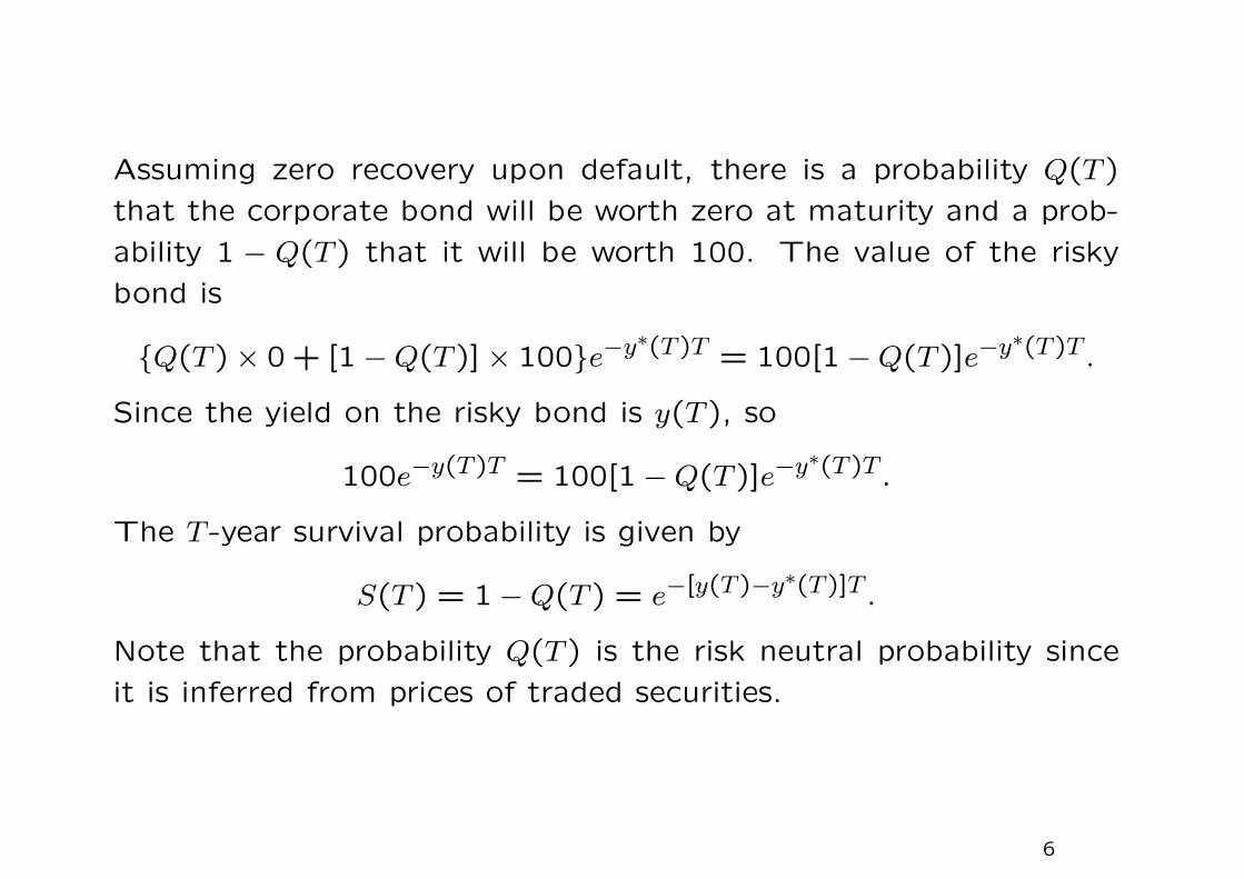
Assuming zero recovery upon default, there is a probability Q(T )

that the corporate bond will be worth zero at maturity and a prob-

ability 1 − Q(T ) that it will be worth 100. The value of the risky

bond is

Q(T )× 0+ [1−Q(T )]× 100e−y∗(T )T = 100[1−Q(T )]e−y∗(T )T .

Since the yield on the risky bond is y(T ), so

100e−y(T )T = 100[1−Q(T )]e−y∗(T )T .

The T -year survival probability is given by

S(T ) = 1−Q(T ) = e−[y(T )−y∗(T )]T .

Note that the probability Q(T ) is the risk neutral probability since

it is inferred from prices of traded securities.

6

As a summary, assuming zero recovery upon default, the survival

probability as implied from the bond prices is seen to be

S(T ) =100e−y(T )T

100e−y∗(T )T=

price of defaultable bond

price of default free bond

= e−credit spread×T ,

where credit spread = y(T )− y∗(T ). Here, the T -year credit spread

is the difference in the yield of the risky zero-coupon and its riskfree

counterpart, both with maturity T .

Alternative proof

Assuming zero recovery and independence of the interest rate pro-

cess and default event, and letting τ be the random default time,

we then have

price of risky bond = E[100e−∫ T0 ru du1τ>T] (zero recovery)

= E[100e−∫ T0 ru du]E[1τ>T] (independence)

= price of riskfree bond× S(T ).

7

Example

Suppose that the spreads over the risk-free rate for 5-year and a 10-

year BBB-rated zero-coupon bonds are 130 and 170 basis points,

respectively, and there is no recovery in the event of default. The

default probabilities can be inferred from the term structure of credit

spreads as follows:

P [τ ≤ 5] = Q(5) = 1− e−0.013×5 = 0.0629

P [τ ≤ 10] = Q(10) = 1− e−0.017×10 = 0.1563.

The probability of default between five years and ten years is Q(5; 10)

where

Q(10) = Q(5) + [(1−Q(5)]Q(5; 10)

or

P [τ ≤ 10|τ > 5] = Q(5; 10) =0.01563− 0.0629

1− 0.0629.

8

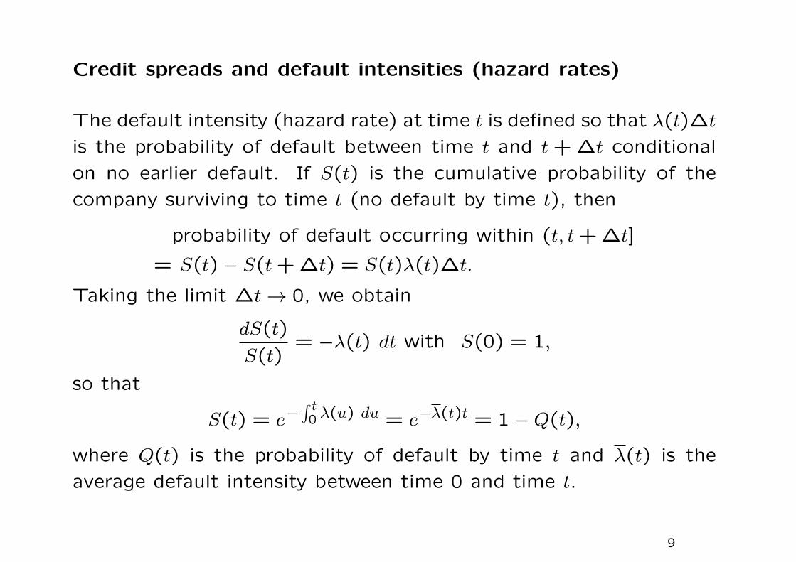
Credit spreads and default intensities (hazard rates)

The default intensity (hazard rate) at time t is defined so that λ(t)∆t

is the probability of default between time t and t + ∆t conditional

on no earlier default. If S(t) is the cumulative probability of the

company surviving to time t (no default by time t), then

probability of default occurring within (t, t+∆t]

= S(t)− S(t+∆t) = S(t)λ(t)∆t.

Taking the limit ∆t → 0, we obtain

dS(t)

S(t)= −λ(t) dt with S(0) = 1,

so that

S(t) = e−∫ t0 λ(u) du = e−λ(t)t = 1−Q(t),

where Q(t) is the probability of default by time t and λ(t) is the

average default intensity between time 0 and time t.

9

• The average default intensity λ(t) can be visualized as the credit

spread over (0, t) since

S(t) = e−[y(t)−y∗(t)]t = e−∫ t0 λ(u) du = e−λ(t)t, t ∈ [0, T ].

• The unconditional default probability density q(t) is defined so

that q(t)∆t gives the probability of default that occurs within

(t, t+∆t). Let F (t) be the distribution function of the random

default time τ , where

F (t) = P [τ ≤ t],

we then have q(t) = F ′(t).

• Recall that q(t)∆t = S(t)λ(t)∆t so that

q(t) = e−∫ t0 λ(u) duλ(t) = S(t)λ(t), t ≥ 0,

where S(t) = 1 − F (t). Also, the probability of surviving until

time t, conditional on survival up to s, where s ≤ t, is given by

P [τ > t|τ > s] =S(t)

S(s)=

e−∫ t0 λ(u) du

e−∫ s0 λ(u) du

= e−∫ ts λ(u) du.

10

Recovery rates

Amounts recovered on corporate bonds as a percent of par valuefrom Moody’s Investor’s Service are shown in the table below.

Class Mean (%) Standard derivation (%)

Senior secured 52.31 25.15

Senior unsecured 48.84 25.01

Senior subordinated 39.46 24.59

Subordinated 33.17 20.78

Junior subordinated 19.69 13.85

The amount recovered is estimated as the market value of the bond

one month after default.

• Seniority of the bond among outstanding bonds issued by the

same issuer is an important determinant of the recovery rate of

that bond. Bonds that are newly issued by an issuer must have

seniority below that of existing bonds issued earlier by the same

issuer.

11

Finite recovery rate

• In the event of a default, the bondholder receives a proportion

R of the bond’s no-default value. If there is no default, then the

bondholder receives 100.

• The bond’s no-default value is 100e−y∗(T )T and the probability

of a default is Q(T ). The value of the bond is

[1−Q(T )]100e−y∗(T )T +Q(T )100Re−y∗(T )T

so that

100e−y(T )T = [1−Q(T )]100e−y∗(T )T +Q(T )100Re−y∗(T )T .

The implied probability of default in terms of yields and recovery

rate is given by

Q(T ) =1− e−[y(T )−y∗(T )]T

1−R.

12

Numerical example on the impact of different assumptions of recov-

ery rates on default probability estimation

Suppose the 1-year default free bond price is $100 and the 1-year

defaultable XY Z corporate bond price is $80.

(i) Assuming R = 0, the probability of default of XY Z as implied

by the two bond prices is

Q0(1) = 1−80

100= 20%.

(ii) Assuming R = 0.6, we obtain

QR(1) =1− 80

100

1− 0.6=

20%

0.4= 50%.

The ratio of Q0(1) : QR(1) = 1 : 11−R.

13

Calculation of default intensity with non-zero recovery rate

Consider a 5-year risky corporate bond that pays a coupon of 6%

per annum (paid semiannually)

• Yield on the corporate bond is 7% per annum (with continuous

compounding)• Yield on a similar risk-free bond is 5% per annum (with contin-

uous compounding)

The yields imply that

(i) price of the riskfree bond

= 3e−0.05×0.5 +3e−0.05×1 + . . .+3e−0.05×4.5 +103e−0.05×5

= 104.09.

(ii) price of the risky bond

= 3e−0.07×0.5 +3e−0.07×1 + . . .+3e−0.07×4.5 +103e−0.07×5

= 95.34.

The present value of expected loss from default over the 5-year life

of the bond = 104.09− 95.34 = 8.75.

14

Let Q denote the constant unconditional probability of default per

year. Assuming that defaults can happen at times 0.5,1.5,2.5,3.5

and 4.5 year (immediately before coupon payment dates), we can

calculate the expected loss from default in terms of Q.

Calculation of loss from default on a bond in terms of the default probability peryear, Q. Notional principal = $100.

Time Default Recovery Risk-free Loss given Discount PV of expected

(years) probability amount($) value($) default($) factor loss($)

0.5 Q 40 106.73 66.73 0.9753 65.08Q

1.5 Q 40 105.97 65.97 0.9277 61.20Q

2.5 Q 40 105.17 65.17 0.8825 57.52Q

3.5 Q 40 104.34 64.34 0.8395 54.01Q

4.5 Q 40 103.46 63.46 0.7985 50.67Q

Total 288.48Q

15

Consider the 3.5 year row in the table.

• The expected value of the riskfree bond at Year 3.5 (time to

expiry is 1.5 years) is

3 + 3e−0.05×0.5 +3e−0.05×1.0 +103e−0.05×1.5 = 104.34.

• The amount recovered if there is a default is 40, so the loss

given default is 104.34− 40 = 64.34.

• The present value of this loss = 64.34×e−0.05×3.5×Q = 64.34×0.8395×Q = 54.01Q.

The total expected loss is 288.48Q. Setting this equal to 8.75, we

obtain Q = 3.03%.

16

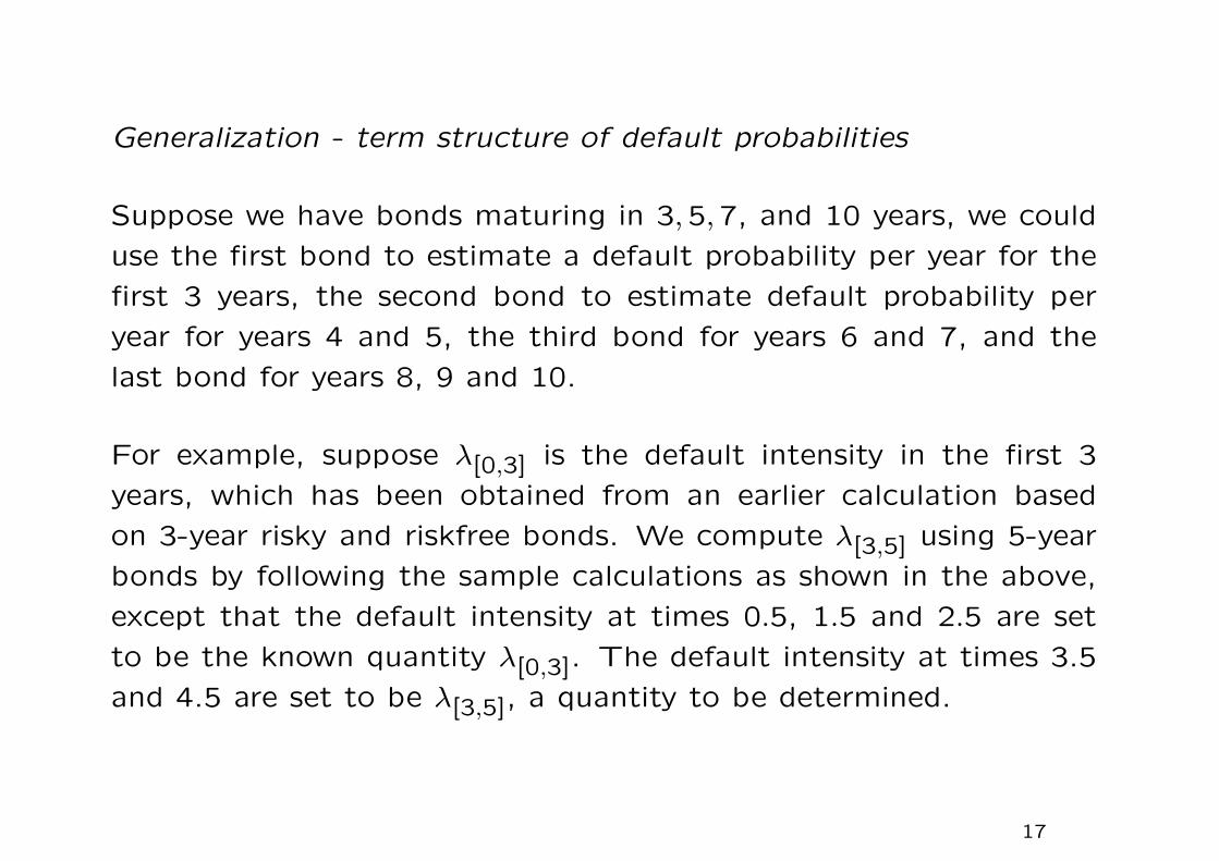
Generalization - term structure of default probabilities

Suppose we have bonds maturing in 3,5,7, and 10 years, we could

use the first bond to estimate a default probability per year for the

first 3 years, the second bond to estimate default probability per

year for years 4 and 5, the third bond for years 6 and 7, and the

last bond for years 8, 9 and 10.

For example, suppose λ[0,3] is the default intensity in the first 3

years, which has been obtained from an earlier calculation based

on 3-year risky and riskfree bonds. We compute λ[3,5] using 5-year

bonds by following the sample calculations as shown in the above,

except that the default intensity at times 0.5, 1.5 and 2.5 are set

to be the known quantity λ[0,3]. The default intensity at times 3.5

and 4.5 are set to be λ[3,5], a quantity to be determined.

17

Construction of a credit risk adjusted yield curve is hindered by

1. The general absence in money markets of liquid traded instru-

ments on credit spread. In recent years, for some liquidly traded

corporate bonds, we may have good liquidity on trading of credit

default swaps whose underlying is the credit spread.

2. The absence of a complete term structure of credit spreads as

implied from traded corporate bonds. At best we only have

infrequent data points.

18

The default probabilities estimated from historical data are much

less than those derived from bond prices

For example, from historical data published by Moody’s, an A-rated

company has average cumulative default rate Q(7) of 0.0091 =

0.91%. The average 7-year default intensity λ(7) is determined by

S(7) = 1− 0.0091 = 0.9909 = e−λ(7)×7

so that

λ(7) = −1

7ln 0.9909 = 0.0013 = 0.13%.

On the other hand, based on bond yields published by Merrill Lynch,

the average Merrill Lynch yield for A-rated bonds was 6.274%.

The average riskfree rate was estimated to be 5.505%. As an ap-

proximation, the average 7-year default intensity is

0.06274− 0.05505

1− 0.4= 0.0128 = 1.28%.

Here, the recovery rate is assumed to be 0.4.

19

Seven-year average default intensities (% per annum).

Rating Historical default Default intensity Ratio Difference

intensity from bonds

Aaa 0.04 0.67 16.8 0.63

Aa 0.06 0.78 13.0 0.72

A 0.13 1.28 9.8 1.15

Baa 0.47 2.38 5.1 1.91

Ba 2.40 5.07 2.1 2.67

B 7.49 9.02 1.2 1.53

Caa 16.90 21.30 1.3 4.40

• Corporate bonds are relatively illiquid and bond traders demand

an extra return to compensate for this.

• Bonds do not default independently of each other. This gives

rise to risk that cannot be diversified away, so bond traders

should require an expected excess return for bearing the risk.

20

Implied default probabilities (equity-based versus credit-based)

• Recovery rate has a significant impact on the defaultable bond

prices. The forward probability of default as implied from the

defaultable and default free bond prices requires estimation of

the expected recovery rate (an almost impossible job).

• The industrial code mKMV estimates default probability using

stock price dynamics – equity-based implied default probability.

For example, the JAL stock price dropped to U1 in early 2010.

Obviously, the equity-based default probability over one year horizon

is close to 100% (stock holders receive almost nothing upon JAL’s

default). However, the credit-based default probability as implied by

the JAL bond prices is less than 30% since the bond par payments

are somewhat partially guaranteed even in the event of default.

21

1.2 Credit default swaps

The protection seller receives fixed periodic payments from the pro-

tection buyer in return for making a single contingent payment cov-

ering losses on a reference asset following a default.

protection

seller

protection

buyer

140 bp per annum

Credit event payment

(100% recovery rate)

only if credit event occurs

holding a

risky bond

22

Protection seller

• earns premium income with no funding cost

• gains customized, synthetic access to the risky bond

Protection buyer

• hedges the default risk on the reference asset

1. Very often, the bond tenor is longer than the swap tenor. In

this way, the protection seller does not have exposure to the full

period of the bond.

2. Basket default swap – gain additional premium by selling default

protection on several assets.

23

A bank lends 10mm to a corporate client at L + 65bps. The bank

also buys 10mm default protection on the corporate loan for 50bps.

Objective achieved by the Bank through the default swap:

• maintain relationship with the corporate borrower

• reduce credit risk on the new loan

Corporate

BorrowerBank Financial

House

Risk Transfer

Interest and

Principal

Default Swap

Premium

If Credit Event:

par amount

If Credit Event:

obligation (loan)

Default swap settlement following Credit Event of Corporate Borrower

24

Settlement of compensation payment

1. Physical settlement:

The defaultable bond is put to the Protection Seller in return

for the par value of the bond.

2. Cash compensation:

An independent third party determines the loss upon default

at the end of the settlement period (say, 3 months after the

occurrence of the credit event).

Compensation amount = (1 − recovery rate) × bond par.

25

Selling protection

To receive credit exposure for a fee (simple credit default swaps) or

in exchange for credit exposure to better diversify the credit portfolio

(exchange credit default swaps).

Buying protection

To reduce either individual credit exposures or credit concentrations

in portfolios. Synthetically to take a short position in an asset

which are not desired to sell outright, perhaps for relationship or

tax reasons.

26

Funding cost arbitrage

Should the Protection Buyer look for a Protection Seller who has a

higher/lower credit rating than himself?

50bpsannual

premium

A-rated institution

as Protection SellerAAA-rated institution

as Protection Buyer

Lender to the

AAA-rated

Institution

LIBOR-15bpsas funding

cost

BBB risky

reference asset

Lender to the

A-rated Institution

coupon

= LIBOR + 90bps

funding cost of

LIBOR + 50bps

27

The combined risk faced by the Protection Buyer:

• default of the BBB-rated bond

• default of the Protection Seller on the contingent payment

Consider the S&P’s Ratings for jointly supported obligations (the

two credit assets are uncorrelated)

A+ A A− BBB+ BBBA+ AA+ AA+ AA+ AA AAA AA+ AA AA AA− AA−

The AAA-rated Protection Buyer creates a synthetic AA−asset with

a coupon rate of LIBOR + 90bps − 50bps = LIBOR + 40bps.

This is better than LIBOR + 30bps, which is the coupon rate of a

AA−asset (net gains of 10bps).

28

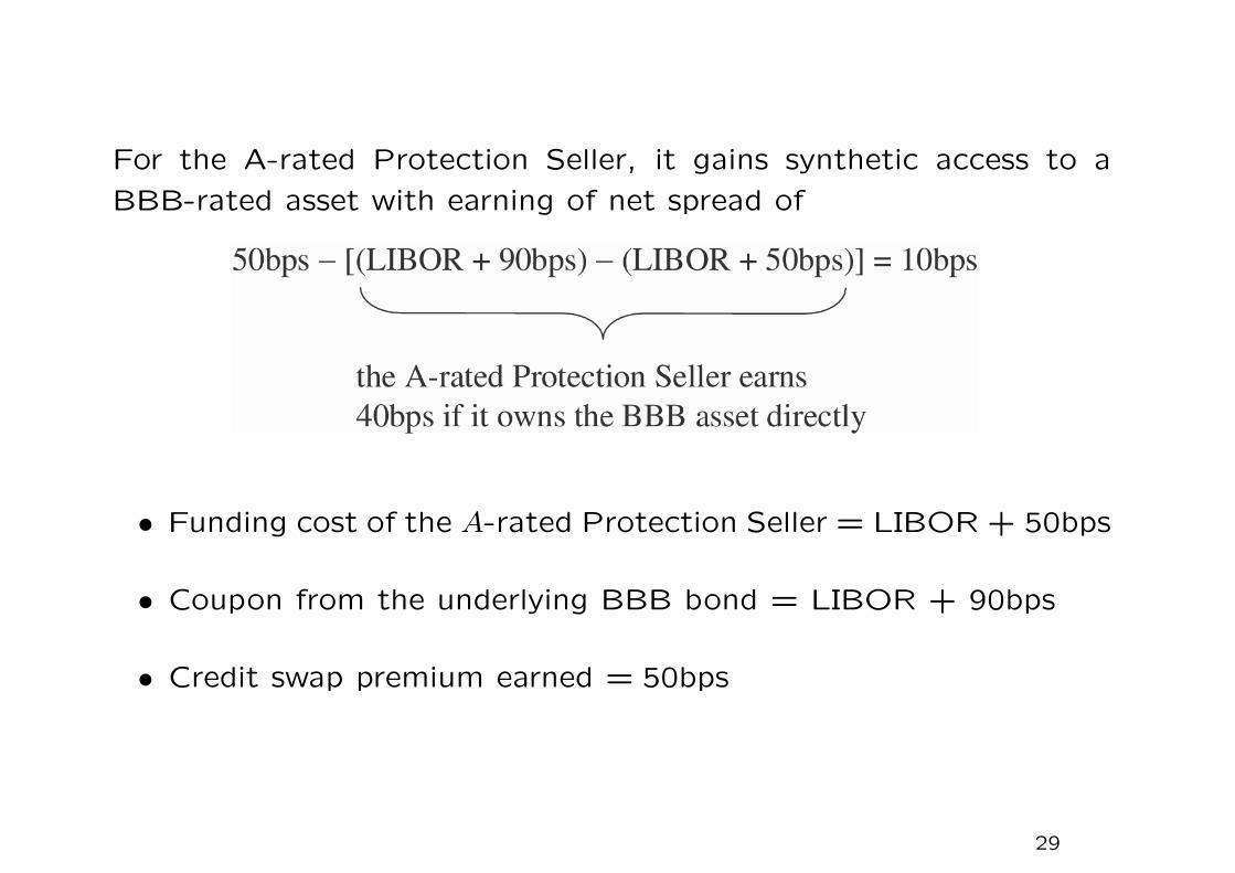
For the A-rated Protection Seller, it gains synthetic access to a

BBB-rated asset with earning of net spread of

• Funding cost of the A-rated Protection Seller = LIBOR + 50bps

• Coupon from the underlying BBB bond = LIBOR + 90bps

• Credit swap premium earned = 50bps

29

In order that the credit arbitrage works, the funding cost of the

default protection seller must be higher than that of the default

protection buyer.

Example

Suppose the A-rated institution is the Protection Buyer, and assume

that it has to pay 60bps for the credit default swap premium (higher

premium since the AAA-rated institution has lower counterparty

risk).

spread earned from holding the risky bond

= coupon from bond − funding cost

= (LIBOR + 90bps) − (LIBOR + 50bps) = 40bps

which is lower than the credit swap premium of 60bps paid for

hedging the credit exposure. No deal is done!

30

Counterparty risk in CDS

Before the Fall 1997 crisis, several Korean banks were willing to

offer credit default protection on other Korean firms.

US commercial

bank

Hyundai

(not rated)

Korea exchange

bank

LIBOR + 70bp

40 bp

Higher geographical risks lead to higher default correlations.

⋆ Higher geographic risks lead to higher default correlations.

Advice: Go for a European bank to buy the protection.

31

How does the inter-dependent default risk structure between the

Protection Seller and the Reference Obligor affect the credit swap

premium rate?

1. Replacement cost (Seller defaults earlier)

• If the Protection Seller defaults prior to the Reference En-

tity, then the Protection Buyer renews the CDS with a new

counterparty.

• Supposing that the default risks of the Protection Seller and

Reference Entity are positively correlated, then there will be

an increase in the swap rate of the new CDS.

2. Settlement risk (Reference Entity defaults earlier)

• The Protection Seller defaults during the settlement period

after the default of the Reference Entity.

32

Hedge strategy using fixed-coupon bonds

Portfolio 1

• One defaultable coupon bond C; coupon c, maturity tN .• One CDS on this bond, with CDS spread s

The portfolio is unwound after a default.

Portfolio 2

• One default-free coupon bond C: with the same payment dates

as the defaultable coupon bond and coupon size c− s.

The default free bond is sold after default of the defaultable coun-

terpart.

33

Comparison of cash flows of the two portfolios

1. In survival, the cash flows of both portfolio are identical.

Portfolio 1 Portfolio 2t = 0 −C(0) −C(0)t = ti c− s c− st = tN 1+ c− s 1+ c− s

2. At default, portfolio 1’s value = par = 1 (full compensation by

the CDS); that of portfolio 2 is C(τ), τ is the time of default.

The price difference at default = 1 − C(τ). This difference is

very small when the default-free bond is a par bond.

Remark

The issuer can choose c to make the bond be a par bond such that

the initial value of the bond is at par.

34

This is an approximate replication.

Recall that the value of the CDS at time 0 is zero. Let B(0, tN)

denote the price of a zero-coupon default-free bond. Neglecting

the difference in the values of the two portfolios at default, the

no-arbitrage principle dictates

C(0) = C(0) = B(0, tN) + cA(0)− sA(0).

Here, (c − s)A(0) is the sum of present value of the coupon pay-

ments at the fixed coupon rate c − s. The equilibrium CDS rate s

can be solved:

s =B(0, tN) + cA(0)− C(0)

A(0).

B(0, tN) + cA(0) is the time-0 price of a default free coupon bond

paying coupon at the rate of c.

35

Cash-and-carry arbitrage with par floater

A par floater C′ is a defaultable bond with a floating-rate coupon

of ci = Li−1 + spar, where the par spread spar is adjusted such that

at issuance the par floater is valued at par.

Portfolio 1

• One defaultable par floater C′ with spread spar over LIBOR.

• One CDS on this bond: CDS spread is s.

The portfolio is unwound after default.

36

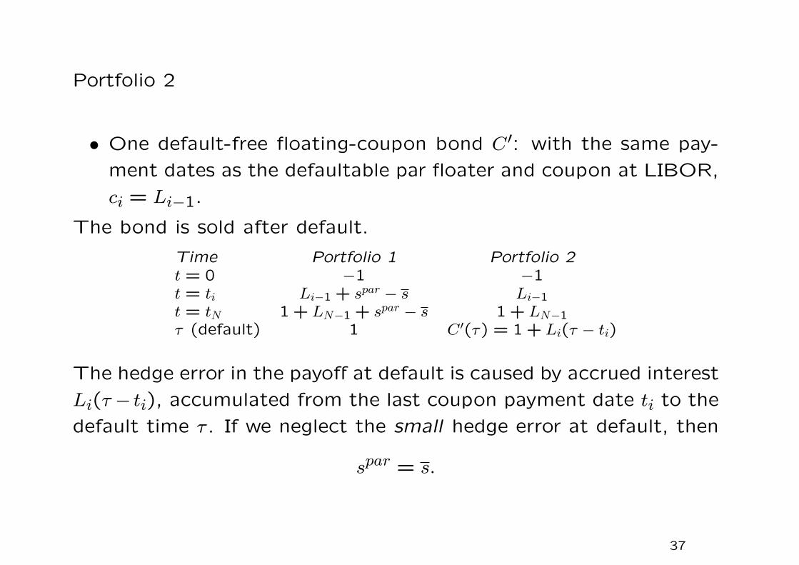
Portfolio 2

• One default-free floating-coupon bond C′: with the same pay-

ment dates as the defaultable par floater and coupon at LIBOR,

ci = Li−1.

The bond is sold after default.

Time Portfolio 1 Portfolio 2t = 0 −1 −1t = ti Li−1 + spar − s Li−1

t = tN 1+ LN−1 + spar − s 1+ LN−1

τ (default) 1 C ′(τ) = 1+ Li(τ − ti)

The hedge error in the payoff at default is caused by accrued interest

Li(τ − ti), accumulated from the last coupon payment date ti to the

default time τ . If we neglect the small hedge error at default, then

spar = s.

37

Remarks

• The non-defaultable bond becomes a par bond (with initial value

equals the par value) when it pays the floating rate equals LI-

BOR. The extra coupon spar paid by the defaultable par floater

represents the credit spread demanded by the investor due to

the potential credit risk. The above result shows that the credit

spread spar is just equal to the CDS spread s.

• The above analysis neglects the counterparty risk of the Pro-

tection Seller of the CDS. Due to potential counterparty risk,

the actual CDS spread will be lower.

38

Valuation of Credit Default Swap

• Suppose that the probability of a reference entity defaulting

during a year conditional on no earlier default is 2%. That is,

the default intensity is assumed to be the constant 2%.

• Table 1 shows the survival probabilities and forward default prob-

abilities (i.e., default probabilities as seen at time zero) for each

of the 5 years. The probability of a default during the first year

is 0.02 and the probability that the reference entity will survive

until the end of the first year is 0.98.

• The forward probability of a default during the second year is

0.02×0.98 = 0.0196 and the probability of survival until the end

of the second year is 0.98× 0.98 = 0.9604.

39

Table 1 Forward default probabilities and survival probabilities

Time (years) Default probability Survival probability

1 0.0200 0.9800

2 0.0196 0.9604 = 0.982

3 0.0192 0.9412 = 0.983

4 0.0188 0.9224 = 0.984

5 0.0184 0.9039 = 0.985

P [3 < τ ≤ 4]

= forward default probability of default during the fourth year (as

seen at current time)

= P [τ > 3]× P [3 < τ ≤ 4|τ > 3]

= survival probability until end of Year 3 × conditional probability

of default in Year 4

= 0.983 × 0.02 = 0.9412× 0.02 = 0.0188.

40

Assumptions on default and recovery rate

We will assume the defaults always happen halfway through a year

and that payments on the credit default swap are made once a year,

at the end of each year. We also assume that the risk-free (LIBOR)

interest rate is 5% per annum with continuous compounding and

the recovery rate is 40%.

Expected present value of CDS premium payments

Table 2 shows the calculation of the expected present value of the

payments made on the CDS assuming that payments are made at

the rate of s per year and the notional principal is $1.

For example, there is a 0.9412 probability that the third payment

of s is made. The expected payment is therefore 0.9412s and its

present value is 0.9412se−0.05×3 = 0.8101s. The total present value

of the expected payments is 4.0704s.

41

Table 2 Calculation of the present value of expected payments.

Payment = s per annum.

Time

(years)

Probability

of survival

Expected

payment

Discount

factor

PV of expected

payment

1 0.9800 0.9800s 0.9512 0.9322s

2 0.9604 0.9604s 0.9048 0.8690s

3 0.9412 0.9412s 0.8607 0.8101s

4 0.9224 0.9224s 0.8187 0.7552s

5 0.9039 0.9039s 0.7788 0.7040s

Total 4.0704s

42

Table 3 Calculation of the present value of expected payoff. No-

tional principal = $1.

Time(years)

Probabilityof default

Recoveryrate

Expectedpayoff ($)

Discountfactor

PV of expectedpayoff ($)

0.5 0.0200 0.4 0.0120 0.9753 0.0117

1.5 0.0196 0.4 0.0118 0.9277 0.0109

2.5 0.0192 0.4 0.0115 0.8825 0.0102

3.5 0.0188 0.4 0.0113 0.8395 0.0095

4.5 0.0184 0.4 0.0111 0.7985 0.0088

Total 0.0511

For example, there is a 0.0192 probability of a payoff halfway through

the third year. Given that the recovery rate is 40%, the expected

payoff at this time is 0.0192× 0.6× 1 = 0.0115. The present value

of the expected payoff is 0.0115e−0.05×2.5 = 0.0102.

The total present value of the expected payoffs is $0.0511.

43

• When default occurs in mid-year, the Protection Buyer has to

pay the premium accrued half year (between the last premium

payment date and default time).

Table 4 Calculation of the present value of accrual payment.

Time

(years)

Probability

of default

Expected

accrual

payment

Discount

factor

PV of ex-

pected accrual

payment

0.5 0.0200 0.0100s 0.9753 0.0097s

1.5 0.0196 0.0098s 0.9277 0.0091s

2.5 0.0192 0.0096s 0.8825 0.0085s

3.5 0.0188 0.0094s 0.8395 0.0079s

4.5 0.0184 0.0092s 0.7985 0.0074s

Total 0.0426s

44

As a final step we evaluate in Table 4 the accrual payment made in

the event of a default.

• There is a 0.0192 probability that there will be a final accrual

payment halfway through the third year.

• The accrual payment is 0.5s.

• The expected accrual payment at this time is therefore 0.0192×0.5s = 0.0096s.

• Its present value is 0.0096se−0.05×2.5 = 0.0085s.

• The total present value of the expected accrual payments is

0.0426s.

From Tables 2 and 4, the present value of the expected payment is

4.0704s+0.0426s = 4.1130s.

45

Equating expected CDS premium payments and expected compen-

sation payment

From Table 3, the present value of the expected payoff is 0.0511.

Equating the two, we obtain the CDS spread for a new CDS as

4.1130s = 0.0511

or s = 0.0124. The mid-market spread should be 0.0124 times the

principal or 124 basis points per year.

In practice, we are likely to find that calculations are more extensive

than those in Tables 2 to 4 because

(a) payments are often made more frequently than once a year

(b) we might want to assume that defaults can happen more fre-

quently than once a year.

46

Impact of expected recovery rate R on credit swap premium s

Recall that the expected compensation payment paid by the Pro-

tection Seller is (1−R)× notional. Therefore, the Protection Seller

charges a higher s if her estimation of the recovery rate R is lower.

Let sR denote the credit swap premium when the recovery rate is

R. We deduce that

s10s50

=(100− 10)%

(100− 50)%=

90%

50%= 1.8.

Remark

A binary credit default swap pays the full notional upon default

of the reference asset. The credit swap premium of a binary swap

depends only on the estimated default probability but not on the

recovery rate.

47

Marking-to-market a CDS

• At the time it is negotiated, a CDS, like most swaps, is worth

zero. Later, it may have a positive or negative value.

• Suppose, for example the credit default swap in our example

had been negotiated some time ago for a spread of 150 basis

points, the present value of the payments by the buyer would be

4.1130 × 0.0150 = 0.0617 and the present value of the payoff

would be 0.0511.

• The value of swap to the seller would therefore be 0.0617 −0.0511, or 0.0166 times the principal.

• Similarly the mark-to-market value of the swap to the buyer of

protection would be −0.0106 times the principal.

48

Basket default swaps

The credit event to insure against using the kth-to-default credit

default swap is the event of the kth default. A premium or spread

s is paid as an insurance fee until maturity or the event of the

kth default, whichever comes first. If the kth default occurs before

swap’s maturity, the Protection Buyer puts the defaulting bond to

the Protection Seller in exchange for the face value of the bond.

Sum of the kth-to-default swap spreads, k = 1,2, . . . , n, for n obligors

in total in the basket is greater than the sum of the individual spreads

of the same set of n obligors:

n∑k=1

sk >n∑

i=1

si.

Why? Apparently, both sides insure exactly the same set of risks:

the n defaults in the basket. At the time of the first default, the

left side stops paying the huge spread s1 while on the plain-vanilla

side one just stops paying the spread si of the first default that falls

on obligor i.

49

Bounds on the swap premiums for the first-to-default (FtD) swaps

under low default correlation

Assuming all 3 obligors have the same dollar exposure, we have

fee on CDS on ≤ fee on FtD ≤ portfolio ofworst credit swap CDSs on all

creditssC ≤ sFtD ≤ sA + sB + sC

With low default probabilities and low default correlation, we have

sFtD ≈ sA + sB + sC.

To see this, by assuming zero default correlation, the probability of

at least one default is

p = 1− (1− pA)(1− pB)(1− pC)

= pA + pB + pC − (pApB + pApC + pBpC) + pApBpC

so that

p / pA + pB + pC for small pA, pB and pC.

50

1.3 Credit spread and bond price based pricing

Market’s assessment of the default risk of the obligor (assuming

some form of market efficiency – information is aggregated in the

market prices). The sources are

• market prices of bonds and other defaultable securities issued

by the obligor• prices of CDS’s referencing this obligor’s credit risk

How to construct a clean term structure of credit spreads from

observed market prices?

51

Based on no-arbitrage pricing principle, a model that is based upon

and calibrated to the prices of traded assets is immune to simple

arbitrage strategies using these traded assets.

Market instruments used in bond price-based pricing

• At time t, the defaultable and default-free zero-coupon bond

prices of all maturities T ≥ t are known. These defaultable

zero-coupon bonds have no recovery at default.

• Information about the probability of default over all time hori-

zons as assessed by market participants are fully reflected when

market prices of default-free and defaultable bonds of all matu-

rities are available.

52

Risk neutral probabilities

The financial market is modeled by a filtered probability space (Ω,

(Ft)t≥0,F , Q), where Q is the risk neutral probability measure.

• All probabilities and expectations are taken under Q. Probabili-

ties are considered as state prices.

1. For constant interest rates, the discounted Q-probability of

an event A at time T is the price of a security that pays off

$1 at time T if A occurs.

2. Under stochastic interest rates, the price of the contingent

claim associated with A is E[β(T )1A], where β(T ) is the dis-

count factor. This is based on the risk neutral valuation prin-

ciple and the money market account M(T ) =1

β(T )= e

∫ Tt ru du

is used as the numeraire.

53

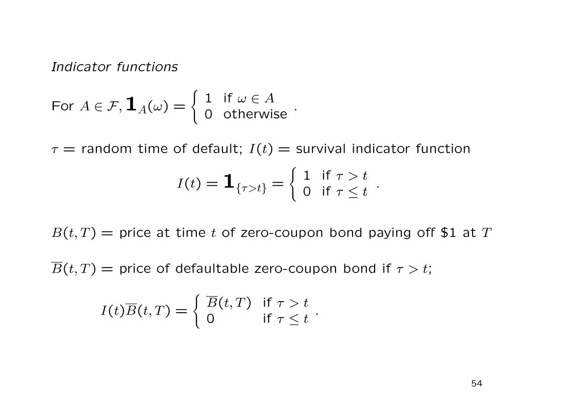
Indicator functions

For A ∈ F ,1A(ω) =

1 if ω ∈ A0 otherwise

.

τ = random time of default; I(t) = survival indicator function

I(t) =1τ>t =

1 if τ > t0 if τ ≤ t

.

B(t, T ) = price at time t of zero-coupon bond paying off $1 at T

B(t, T ) = price of defaultable zero-coupon bond if τ > t;

I(t)B(t, T ) =

B(t, T ) if τ > t0 if τ ≤ t

.

54

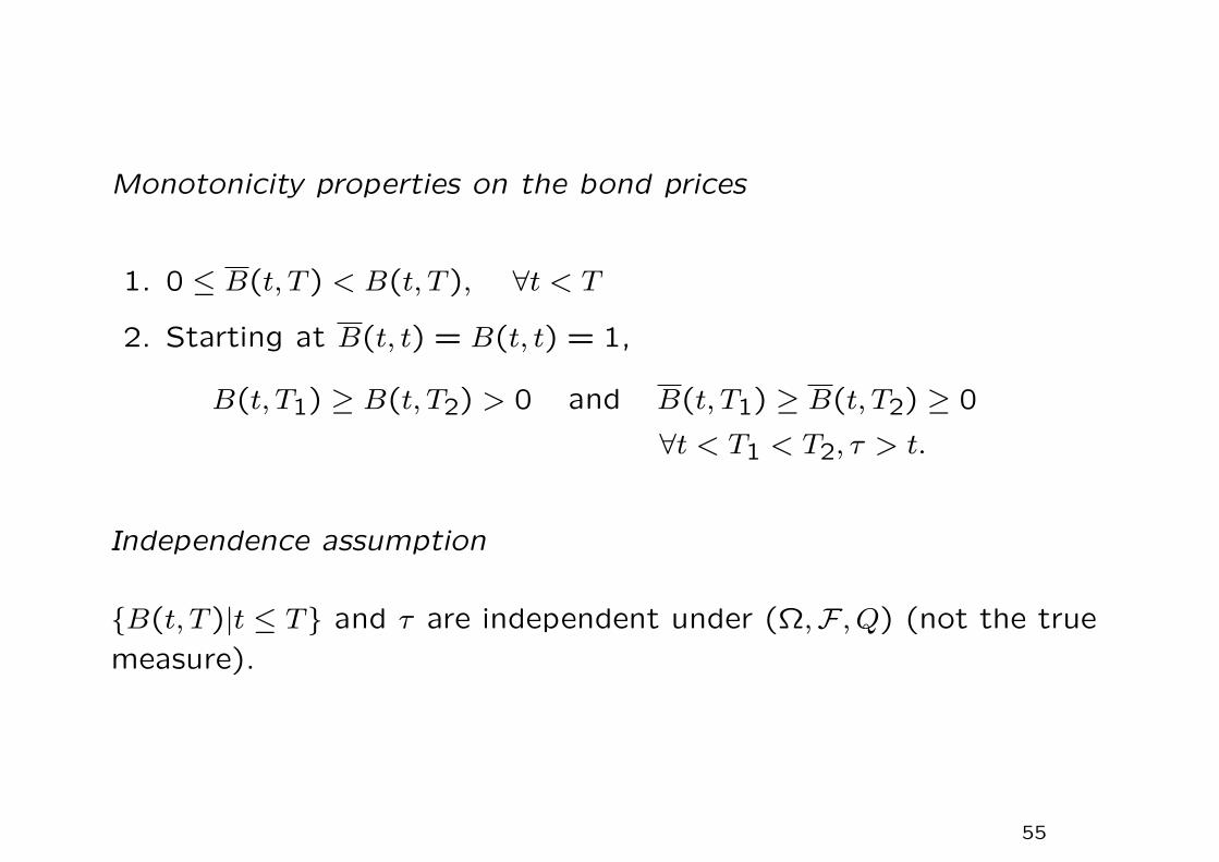
Monotonicity properties on the bond prices

1. 0 ≤ B(t, T ) < B(t, T ), ∀t < T

2. Starting at B(t, t) = B(t, t) = 1,

B(t, T1) ≥ B(t, T2) > 0 and B(t, T1) ≥ B(t, T2) ≥ 0

∀t < T1 < T2, τ > t.

Independence assumption

B(t, T )|t ≤ T and τ are independent under (Ω,F , Q) (not the true

measure).

55

Implied probability of survival in [t, T ]– based on market prices

of bonds

B(t, T ) = E

[e−∫ Tt ru du

]and B(t, T ) = E

[e−∫ Tt ru duI(T )

].

Invoking the independence between defaults and the default-free

interest rates

B(t, T ) = E

[e−∫ Tt ru du

]E[I(T )] = B(t, T )P (t, T )

implied survival probability over [t, T ] = P (t, T ) =B(t, T )

B(t, T ).

56

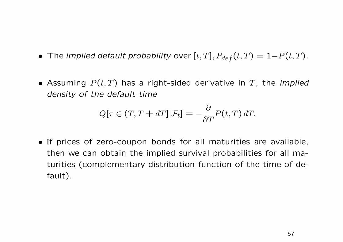
• The implied default probability over [t, T ], Pdef(t, T ) = 1−P (t, T ).

• Assuming P (t, T ) has a right-sided derivative in T , the implied

density of the default time

Q[τ ∈ (T, T + dT ]|Ft] = −∂

∂TP (t, T ) dT.

• If prices of zero-coupon bonds for all maturities are available,

then we can obtain the implied survival probabilities for all ma-

turities (complementary distribution function of the time of de-

fault).

57

Properties on implied survival probabilities, P (t, T )

1. P (t, t) = 1 and it is non-negative and decreasing in T . Also,

P (t,∞) = 0.2. Normally P (t, T ) is continuous in its second argument, except

that an important event secheduled at some time T1 has direct

influence on the survival of the obligor.3. Viewed as a function of its first argument t, all survival proba-

bilities for fixed maturity dates will tend to increase.

If we want to focus on the default risk over a given time interval in

the future, we should consider conditional survival probabilities.

conditional survival probability over [T1, T2] as seen from t

= P (t, T1, T2) =P (t, T2)

P (t, T1), where t ≤ T1 < T2.

58

Implied hazard rate (default probabilities per unit time interval length)

Discrete implied hazard rate of default over (T, T + ∆T ] as seen

from time t

H(t, T, T +∆T )∆T =P (t, T )

P (t, T +∆T )− 1 =

Pdef(t, T, T +∆T )

P (t, T, T +∆T ),

so that

P (t, T ) = P (t, T +∆T )[1 +H(t, T, T +∆T )∆T ].

In the limit of ∆T → 0, the continuous hazard rate at time T as

seen at time t is given by

h(t, T ) = −∂

∂TlnP (t, T ).

59

Proof First, we recall

1

P (t, T, T +∆T )=

P (t, T )

P (t, T, T +∆T ).

We have

h(t, T ) = lim∆T→0

H(t, T, T +∆T )

= lim∆T→0

1− P (t, T, T +∆T )

∆TP (t, T, T +∆T )

= lim∆T→0

1

∆T

[P (t, T )

P (t, T +∆T )− 1

]

= lim∆T→0

−1

P (t, T +∆T )

P (t, T +∆T )− P (t, T )

∆T

= −1

P (t, T )

∂

∂TP (t, T )

= −∂

∂TlnP (t, T ).

60

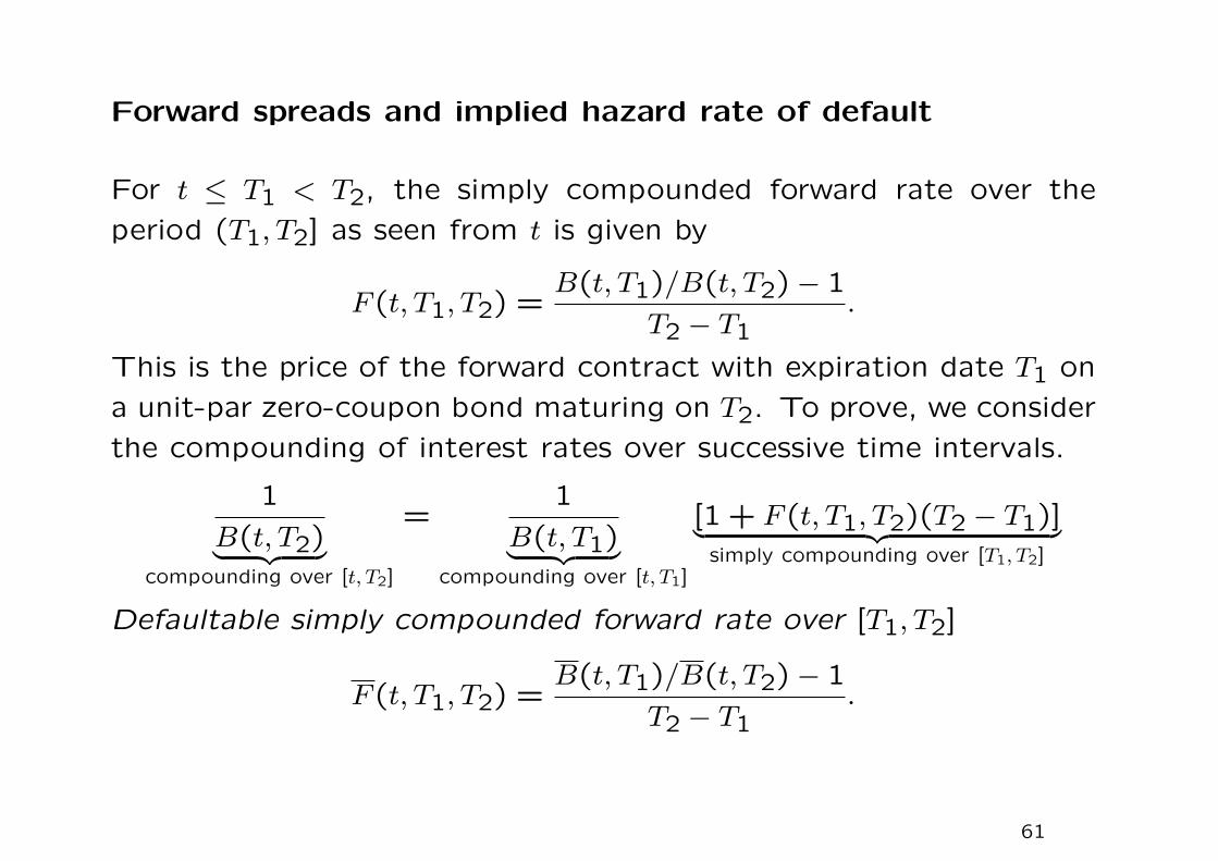
Forward spreads and implied hazard rate of default

For t ≤ T1 < T2, the simply compounded forward rate over the

period (T1, T2] as seen from t is given by

F (t, T1, T2) =B(t, T1)/B(t, T2)− 1

T2 − T1.

This is the price of the forward contract with expiration date T1 on

a unit-par zero-coupon bond maturing on T2. To prove, we consider

the compounding of interest rates over successive time intervals.

1

B(t, T2)︸ ︷︷ ︸compounding over [t, T2]

=1

B(t, T1)︸ ︷︷ ︸compounding over [t, T1]

[1 + F (t, T1, T2)(T2 − T1)]︸ ︷︷ ︸simply compounding over [T1, T2]

Defaultable simply compounded forward rate over [T1, T2]

F (t, T1, T2) =B(t, T1)/B(t, T2)− 1

T2 − T1.

61

Instantaneous continuously compounded forward rates

f(t, T ) = lim∆T→0

F (t, T, T +∆T ) = −∂

∂TlnB(t, T )

f(t, T ) = lim∆T→0

F (t, T, T +∆T ) = −∂

∂TlnB(t, T ).

Implied hazard rate of default

Recall

P (t, T1, T2) =B(t, T2)

B(t, T2)

B(t, T1)

B(t, T1)

=1+ F (t, T1, T2)(T2 − T1)

1 + F (t, T1, T2)(T2 − T1)= 1− Pdef(t, T1, T2),

and upon expanding, we obtain

Pdef(t, T1, T2) [1 + F (t, T1, T2)(T2 − T1)]︸ ︷︷ ︸B(t,T1)/B(t,T2)

= [F (t, T1, T2)−F (t, T1, T2)](T2−T1).

62

Define H(t, T1, T2) =Pdef(t, T1, T2)

(T2 − T1)P (t, T1, T2)as the discrete implied

rate of default. We then have

H(t, T1, T2) =B(t, T2)

B(t, T1)

[F (t, T1, T2)− F (t, T1, T2)]

P (t, T1, T2)

=B(t, T2)

B(t, T1)[F (t, T1, T2)− F (t, T1, T2)].

Taking the limit T2 → T1, then the implied hazard rate of default at

time T > t as seen from time t is the spread between the forward

rates:

h(t, T ) = f(t, T )− f(t, T ).

Alternatively, we obtain the above relation using

f(t, T )− f(t, T ) = −∂

∂Tln

B(t, T )

B(t, T )

= −∂

∂TlnP (t, T ) = h(t, T ).

63

The local default probability at time t over the next small time step

∆t1

∆tQ[τ ≤ t+∆t|Ft ∧ τ > t] ≈ r(t)− r(t) = λ(t)

where r(t) = f(t, t) is the riskfree short rate and r(t) = f(t, t) is the

defaultable short rate.

Recovery value

View an asset with positive recovery as an asset with an additional

positive payoff at default. The recovery value is the expected value

of the recovery shortly after the occurrence of a default.

64

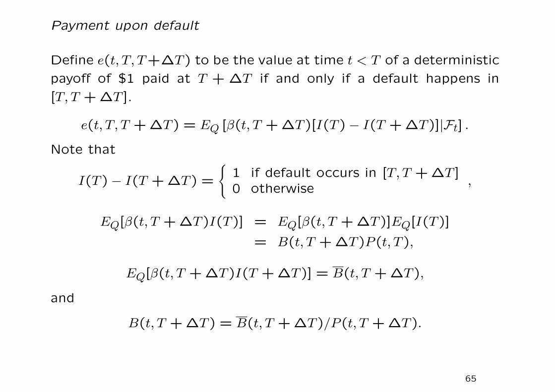
Payment upon default

Define e(t, T, T+∆T ) to be the value at time t < T of a deterministic

payoff of $1 paid at T + ∆T if and only if a default happens in

[T, T +∆T ].

e(t, T, T +∆T ) = EQ [β(t, T +∆T )[I(T )− I(T +∆T )]|Ft] .

Note that

I(T )− I(T +∆T ) =

1 if default occurs in [T, T +∆T ]0 otherwise

,

EQ[β(t, T +∆T )I(T )] = EQ[β(t, T +∆T )]EQ[I(T )]

= B(t, T +∆T )P (t, T ),

EQ[β(t, T +∆T )I(T +∆T )] = B(t, T +∆T ),

and

B(t, T +∆T ) = B(t, T +∆T )/P (t, T +∆T ).

65

It is seen that

e(t, T, T +∆T ) = B(t, T +∆T )P (t, T )−B(t, T +∆T )

= B(t, T +∆T )

[P (t, T )

P (t, T +∆T )− 1

]= ∆TB(t, T +∆T )H(t, T, T +∆T )

On taking the limit ∆T → 0, we obtain

rate of default compensation = e(t, T ) = lim∆T→0

e(t, T, T +∆T )

∆T= B(t, T )h(t, T ) = B(t, T )P (t, T )h(t, T ).

The value of a security that pays π(s) if a default occurs at time s

for all t < s < T is given by∫ T

tπ(s)e(t, s) ds =

∫ T

tπ(s)B(t, s)h(t, s) ds.

This result holds for deterministic recovery rates.

66

Random recovery value

• Suppose the payoff at default is not a deterministic function

π(τ) but a random variable π′ which is drawn at the time of

default τ . π′ is called a marked point process. Define

πe(t, T ) = EQ[π′|Ft ∧ τ = T].

which is the expected value of π′ conditional on default at T and

information at t.• Conditional on a default occurring at time T , the price of a

security that pays π′ at default is B(t, T )πe(t, T ).• Since the time of default is not known, we have to integrate

these values over all possible default times and weight them

with the respective probability of default occurring.• The price at time t of a payoff of π′ at τ if τ ∈ [t, T ] is given by∫ T

tπe(t, s)B(t, s)P (t, s)︸ ︷︷ ︸

B(t,s)

h(t, s) ds.

67

Building blocks for credit derivatives pricing

Tenor structure

δk = Tk+1−Tk,0 ≤ k ≤ K−1

Coupon and repayment dates for bonds, fixing dates for rates, pay-

ment and settlement dates for credit derivatives all fall on Tk,0 ≤k ≤ K.

68

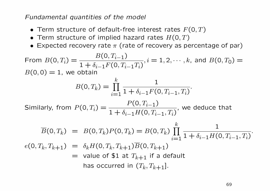
Fundamental quantities of the model

• Term structure of default-free interest rates F (0, T )• Term structure of implied hazard rates H(0, T )• Expected recovery rate π (rate of recovery as percentage of par)

From B(0, Ti) =B(0, Ti−1)

1 + δi−1F (0, Ti−1Ti), i = 1,2, · · · , k, and B(0, T0) =

B(0,0) = 1, we obtain

B(0, Tk) =k∏

i=1

1

1+ δi−1F (0, Ti−1, Ti).

Similarly, from P (0, Ti) =P (0, Ti−1)

1 + δi−1H(0, Ti−1, Ti), we deduce that

B(0, Tk) = B(0, Tk)P (0, Tk) = B(0, Tk)k∏

i=1

1

1+ δi−1H(0, Ti−1, Ti).

e(0, Tk, Tk+1) = δkH(0, Tk, Tk+1)B(0, Tk+1)

= value of $1 at Tk+1 if a default

has occurred in (Tk, Tk+1].

69

Taking the limit δi → 0, for all i = 0,1, · · · , k

B(0, Tk) = exp

(−∫ Tk

0f(0, s) ds

)

B(0, Tk) = exp

(−∫ Tk

0[h(0, s) + f(0, s)] ds

)e(0, Tk) = h(0, Tk)B(0, Tk).

Alternatively, the above relations can be obtained by integrating

f(0, T ) = −∂

∂TlnB(0, T ) with B(0,0) = 1

f(0, T ) = h(0, T ) + f(0, T ) = −∂

∂TlnB(0, T ) with B(0,0) = 1.

70

Defaultable fixed coupon bond

c(0) =K∑

n=1

cnB(0, Tn) (coupon) cn = cδn−1

+ B(0, TK) (principal)

+ πK∑

k=1

e(0, Tk−1, Tk) (recovery)

The recovery payment can be written as

πK∑

k=1

e(0, Tk−1, Tk) =K∑

k=1

πδk−1H(0, Tk−1, Tk)B(0, Tk).

The recovery payments can be considered as an additional coupon

payment stream of πδk−1H(0, Tk−1, Tk).

71

Defaultable floater

Recall that L(Tn−1, Tn) is the reference LIBOR rate applied over

[Tn−1, Tn] at Tn−1 so that 1 + L(Tn−1, Tn)δn−1 is the growth factor

over [Tn−1, Tn]. Application of no-arbitrage argument gives

B(Tn−1, Tn) =1

1+ L(Tn−1, Tn)δn−1.

• The coupon payment at Tn equals LIBOR plus a spread

δn−1[L(Tn−1, Tn) + spar

]=

[1

B(Tn−1, Tn)− 1

]+ sparδn−1.

• Consider the payment of1

B(Tn−1, Tn)at Tn, its value at Tn−1

isB(Tn−1, Tn)

B(Tn−1, Tn)= P (Tn−1, Tn). Why? We use the defaultable

discount factor B(Tn−1, Tn) since the coupon payment may be

defaultable over [Tn−1, Tn].

72

• Seen at t = 0, the value becomes

B(0, Tn−1)P (0, Tn−1, Tn)

= B(0, Tn−1)P (0, Tn−1)P (0, Tn−1, Tn)

= B(0, Tn−1)P (0, Tn).

Combining with the fixed part of the coupon payment and observing

the relation

[B(0, Tn−1)−B(0, Tn)]P (0, Tn) =

[B(0, Tn−1)

B(0, Tn)− 1

]B(0, Tn)

= δn−1F (0, Tn−1, Tn)B(0, Tn),

the model price of the defaultable floating rate bond is

c(0) =K∑

n=1

δn−1F (0, Tn−1, Tn)B(0, Tn) + sparK∑

n=1

δn−1B(0, Tn)

+ B(0, TK) + πK∑

k=1

e(0, Tk−1, Tk).

73

1.4 Pricing of credit derivatives

Credit default swap revisited

Fixed leg Payment of δn−1s at Tn if no default until Tn.

The value of the fixed leg is

sN∑

n=1

δn−1B(0, Tn).

Floating leg Payment of 1 − π at Tn if default in (Tn−1, Tn]

occurs. The value of the floating leg is

(1− π)N∑

n=1

e(0, Tn−1, Tn)

= (1− π)N∑

n=1

δn−1H(0, Tn−1, Tn)B(0, Tn).

74

The market CDS spread is chosen such that the fixed leg and float-

ing leg of the CDS have the same value. Hence

s = (1− π)

N∑n=1

δn−1H(0, Tn−1, Tn)B(0, Tn)∑Nn=1 δn−1B(0, Tn)

.

Define the weights

wn =δn−1B(0, Tn)N∑

k=1

δk−1B(0, Tk)

, n = 1,2, · · · , N, andN∑

n=1

wn = 1,

then the fair swap premium rate is given by

s = (1− π)N∑

n=1

wnH(0, Tn−1, Tn).

75

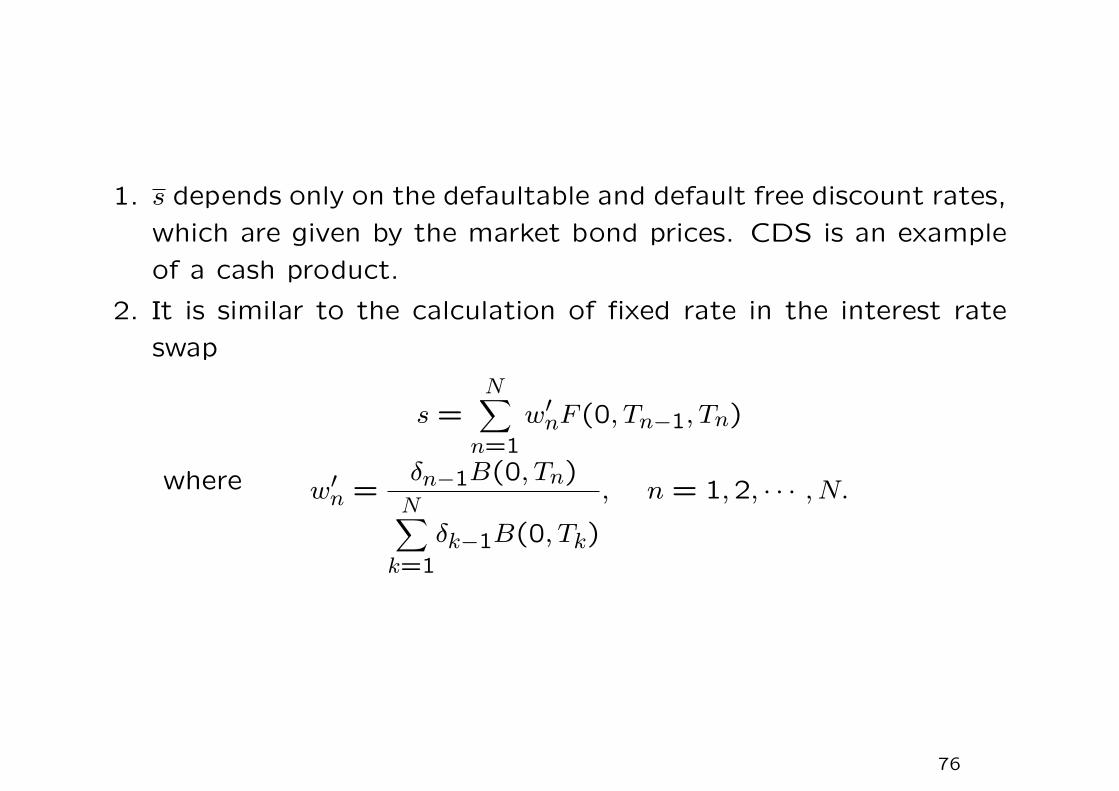
1. s depends only on the defaultable and default free discount rates,

which are given by the market bond prices. CDS is an example

of a cash product.

2. It is similar to the calculation of fixed rate in the interest rate

swap

s =N∑

n=1

w′nF (0, Tn−1, Tn)

where w′n =

δn−1B(0, Tn)N∑

k=1

δk−1B(0, Tk)

, n = 1,2, · · · , N.

76

Marked-to-market value

original CDS spread = s′; new CDS spread = s

Let Π = CDSold − CDSnew, and observe that CDSnew = 0, then

marked-to-market value = CDSold = Π = (s− s′)N∑

n=1

B(0, Tn)δn−1.

Why? If an offsetting trade is entered at the current CDS rate s,

only the fee difference (s − s′) will be received over the life of the

CDS. Should a default occurs, the protection payments will cancel

out, and the fee difference payment will be cancelled, too. The

fee difference stream is defaultable and must be discounted with

B(0, Tn).

• CDS’s are useful instruments to gain exposure against spread

movements, not just against default arrival risk.

77

Hedge based pricing – approximate hedge and replication strate-

gies

Provide hedge strategies that cover much of the risks involved in

credit derivatives – independent of any specific pricing model.

Basic instruments

1. Default free bond

C(t) = time-t price of default-free bond with fixed-coupon C

B(t, T ) = time-t price of default-free zero-coupon bond

2. Defaultable bond

C(t) = time-t price of defaultable bond with fixed-coupon c

C′(t) = time-t price of defaultable bond with floating coupon

LIBOR + spar

78

3. Interest rate swap

S(t) = swap rate at time t of a standard fixed-for-floating

=B(t, tn)−B(t, tN)

A(t; tn, tN), t ≤ tn

where A(t; tn, tN) =N∑

i=n+1

δiB(t, ti) = value of the payment stream

paying δi on each date ti.

Proof of the swap rate formula

The floating rate coupon payments can be generated by putting $1

at tn and taking away the floating interests immediately. At tN ,

$1 remains. The sum of the present value of the floating interests

= B(t, tn)−B(t, tN).

Intuition behind cash-and-carry arbitrage pricing of CDSs

A combined position of a CDS with a defaultable bond C is very

well hedged against default risk.

79

Asset swap packages

An asset swap package consists of a defaultable coupon bond C with

coupon c and an interest rate swap. The bond’s coupon is swapped

into LIBOR plus the asset swap rate sA. Asset swap package is sold

at par.

Remark Asset swap transactions are driven by the desire to strip

out unwanted structured features from the underlying asset.

Payoff streams to the buyer of the asset swap package

time defaultable bond swap nett = 0 −C(0) −1+ C(0) −1t = ti c∗ −c+ Li−1 + sA Li−1 + sA + (c∗ − c)t = tN (1 + c)∗ −c+ LN−1 + sA 1∗ + LN−1 + sA + (c∗ − c)default recovery unaffected recovery

* denotes payment contingent on survival.

80

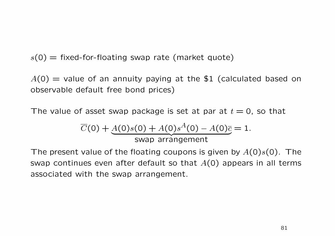
s(0) = fixed-for-floating swap rate (market quote)

A(0) = value of an annuity paying at the $1 (calculated based on

observable default free bond prices)

The value of asset swap package is set at par at t = 0, so that

C(0) +A(0)s(0) +A(0)sA(0)−A(0)c︸ ︷︷ ︸swap arrangement

= 1.

The present value of the floating coupons is given by A(0)s(0). The

swap continues even after default so that A(0) appears in all terms

associated with the swap arrangement.

81

Solving for sA(0)

sA(0) =1

A(0)[1− C(0)] + c− s(0).

Rearranging the terms,

C(0) +A(0)sA(0) = [1−A(0)s(0)] +A(0)c︸ ︷︷ ︸default-free bond

≡ C(0)

where the right-hand side gives the value of a default-free bond with

coupon c. Note that 1 − A(0)s(0) is the present value of receiving

$1 at maturity tN . We obtain

sA(0) =1

A(0)[C(0)− C(0)].

82

Credit spread options

The terminal payoff is given by

Psp(r, s, T ) = max(s−K,0)

where r = riskless interest rate

s = credit spread

K = strike spread

Discrete-time Heath-Jarrow-Morton (HJM) method

• Follows the HJM term structure approach that models the for-

ward rate process and forward spread process for riskless and

risky bonds.

• The model takes the observed term structures of riskfree forward

rates and credit spreads as input information.

• Find the risk neutral drifts of the stochastic processes such that

all discounted security prices are martingales.

83

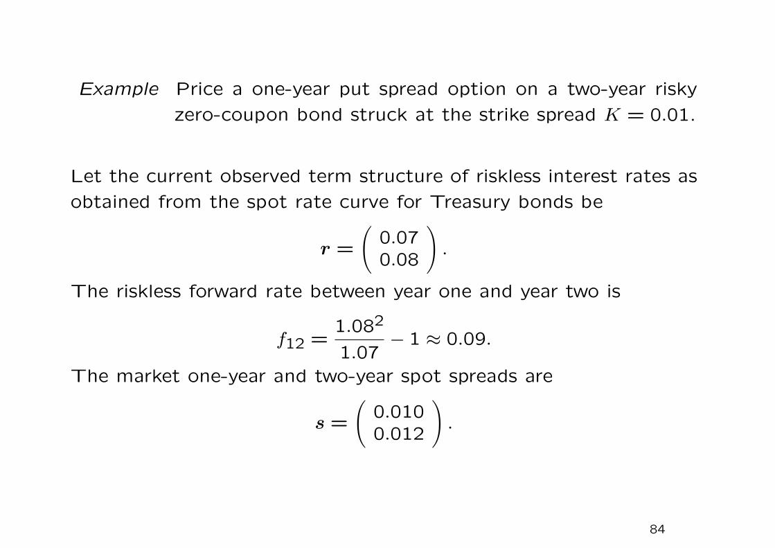
Example Price a one-year put spread option on a two-year risky

zero-coupon bond struck at the strike spread K = 0.01.

Let the current observed term structure of riskless interest rates as

obtained from the spot rate curve for Treasury bonds be

r =

(0.070.08

).

The riskless forward rate between year one and year two is

f12 =1.082

1.07− 1 ≈ 0.09.

The market one-year and two-year spot spreads are

s =

(0.0100.012

).

84

The two-year risky rate is 0.08 + 0.012 = 0.092. The current price

of a risky two-year zero coupon bond with face value $100 is

B(0) = $100/(1.092)2 = $83.86.

• The discrete stochastic process for the spread under the true

measure is assumed to take the form of a square-root process

where the volatility depends on√s(0)

s(∆t) = s(0) + k[θ − s(0)]∆t± σ√s(0)∆t

where k = 0.3, θ = 0.02 and σ = 0.04,∆t = 1, s(0) = 0.01.

85

• We need to add an adjustment term γ in the drift term in order

to risk-adjust the stochastic forward spread process

s(t) = s(0) + k[θ − s(0)]∆t+ γ ± σ√s(0)∆t.

The adjustment term γ is determined by requiring the discounted

bond prices to be martingales.

• Let B(1) denote the price at t = 1 of the risky bond maturing

at t = 2. The forward defaultable discount factor over year one

and year two is1

1 + f12 + s(1), where s(1) is the forward spread

over the period.

s(1) =

γ +0.017γ +0.009

so that B(1) =

100

1+f12+γ+0.017

1001+f12+γ+0.009,

with equal probabilities for assuming the high and low values.

86

We determine γ such that the bond price is a martingale.

B(0) = 83.86 =1

1+ 0.07+ 0.01×

1

2

(100

1.107+ γ+

100

1.099+ γ

).

The first term is the risky defaultable discount factor and the last

term is the expected value of B(1). We obtain γ = 0.0012 so that

s(1) =

0.01820.0102

.

The current value of put spread option is

1

1.07×

1

2[(0.0182− 0.01) + (0.0102− 0.01)]L = 0.00393L,

where L is the notional value of the put spread option. Note that

the default free discount factor 1/1.07 is used in the option value

calculation.

87