
Risk Management in Financial Institutions -...
67
Risk Management in Financial Institutions * Adriano A. Rampini † S. Viswanathan ‡ Guillaume Vuillemey § April 2017 Abstract We study risk management in financial institutions using data on hedging of interest rate and foreign exchange risk. We find strong evidence that better capi- talized institutions hedge more both in the cross-section and within institutions over time. For identification, we exploit net worth shocks resulting from loan losses due to drops in house prices. Institutions that sustain such losses reduce hedging sub- stantially relative to otherwise similar institutions. The evidence is consistent with the theory that financial constraints impede both financing and hedging. We find no evidence that risk shifting, changes in interest rate risk exposures, or regulatory capital explain hedging behavior. Keywords: Risk management; Financial institutions; Interest rate risk; Financial constraints; Derivatives J.E.L. Codes: G21, G32, D92, E44 * We thank Manuel Adelino, Juliane Begenau, Markus Brunnermeier, Mark Flannery, Joao Granja, Divya Kirti, Kebin Ma, Justin Murfin, Dimitris Papanikolaou, Roberta Romano, Farzad Saidi, João Santos, David Scharfstein, Jeremy Stein, René Stulz, Jason Sturgess, Adi Sunderam, Yuri Tserlukevich, James Vickery, and seminar participants at Duke University, HEC Paris, Princeton University, Georgia State University, the Federal Reserve Bank of New York, the NBER Insurance and Corporate Finance Joint Meeting, the FIRS Conference, the NYU-NY Fed-RFS Conference on Financial Intermediation, the ETH-NYU Law & Banking/Finance Conference, the Paul Woolley Centre Conference at LSE, the LBS Summer Finance Symposium, the Barcelona GSE Summer Forum, INSEAD, Frankfurt School of Finance & Management, the CEPR ESSFM in Gerzensee, the EFA Annual Meeting, EIEF, the Wharton Conference on Liquidity and Financial Crises, the AFA Annual Meeting, the Jackson Hole Finance Conference, the NY Fed Conference on OTC Derivatives, NUS, Paris-Dauphine, and Mannheim for helpful comments. First draft: October 2015. Address: Duke University, Fuqua School of Business, 100 Fuqua Drive, Durham, NC, 27708. † Duke University, NBER, and CEPR. Phone: (919) 660-7797. Email: [email protected]. ‡ Duke University and NBER. Phone: (919) 660-7784. Email: [email protected]. § HEC Paris and CEPR. Phone: +33 (0)6 60 20 42 75. Email: [email protected].
Transcript of Risk Management in Financial Institutions -...
Risk Management in Financial Institutions∗
Adriano A. Rampini† S. Viswanathan‡ Guillaume Vuillemey§
April 2017
Abstract
We study risk management in financial institutions using data on hedging ofinterest rate and foreign exchange risk. We find strong evidence that better capi-talized institutions hedge more both in the cross-section and within institutions overtime. For identification, we exploit net worth shocks resulting from loan losses dueto drops in house prices. Institutions that sustain such losses reduce hedging sub-stantially relative to otherwise similar institutions. The evidence is consistent withthe theory that financial constraints impede both financing and hedging. We findno evidence that risk shifting, changes in interest rate risk exposures, or regulatorycapital explain hedging behavior.
Keywords: Risk management; Financial institutions; Interest rate risk; Financialconstraints; DerivativesJ.E.L. Codes: G21, G32, D92, E44
∗We thank Manuel Adelino, Juliane Begenau, Markus Brunnermeier, Mark Flannery, Joao Granja,Divya Kirti, Kebin Ma, Justin Murfin, Dimitris Papanikolaou, Roberta Romano, Farzad Saidi, JoãoSantos, David Scharfstein, Jeremy Stein, René Stulz, Jason Sturgess, Adi Sunderam, Yuri Tserlukevich,James Vickery, and seminar participants at Duke University, HEC Paris, Princeton University, GeorgiaState University, the Federal Reserve Bank of New York, the NBER Insurance and Corporate FinanceJoint Meeting, the FIRS Conference, the NYU-NY Fed-RFS Conference on Financial Intermediation,the ETH-NYU Law & Banking/Finance Conference, the Paul Woolley Centre Conference at LSE, theLBS Summer Finance Symposium, the Barcelona GSE Summer Forum, INSEAD, Frankfurt School ofFinance & Management, the CEPR ESSFM in Gerzensee, the EFA Annual Meeting, EIEF, the WhartonConference on Liquidity and Financial Crises, the AFA Annual Meeting, the Jackson Hole FinanceConference, the NY Fed Conference on OTC Derivatives, NUS, Paris-Dauphine, and Mannheim forhelpful comments. First draft: October 2015. Address: Duke University, Fuqua School of Business, 100Fuqua Drive, Durham, NC, 27708.†Duke University, NBER, and CEPR. Phone: (919) 660-7797. Email: [email protected].‡Duke University and NBER. Phone: (919) 660-7784. Email: [email protected].§HEC Paris and CEPR. Phone: +33 (0)6 60 20 42 75. Email: [email protected].
1 Introduction
The potential of the market for financial derivatives for use in risk management remains
unrealized. Limited risk management leaves financial institutions, firms, and households
more exposed to shocks than they could be and is arguably a key factor in financial
crises. Why the gains from using traded securities for risk management are exploited to
such a limited extent remains a fundamental open question. In this paper, we study the
determinants of risk management in the quantitatively largest market for such instruments
– the interest rate derivatives market – in which the main participants are financial
institutions.
We show that the net worth of financial institutions is a principal determinant of their
risk management: better capitalized institutions hedge more and institutions whose net
worth declines reduce hedging. To study the causal effect of net worth on hedging, we
propose a novel identification strategy; we instrument variation in financial institutions’
net worth using losses on real estate loans attributable to local house price shocks. Using
these shocks to estimate difference-in-differences specifications, we find that institutions
whose net worth drops substantially reduce risk management. We conclude that the
financing needs associated with hedging are a major barrier to risk management.
We focus on the financial intermediary sector for several reasons. First, despite much
debate about bank risk management and its failure during the financial crisis, the ba-
sic patterns of risk management in financial institutions are not known and its main
determinants are not well understood. Second, financial institutions play a key role in
the macroeconomy and for the transmission of monetary policy. Understanding their
exposure to shocks is thus essential for monetary and macro-prudential policy.1 Third,1Following Bernanke and Gertler (1989), the effects of the net worth of financial institutions on the
availability of intermediated finance and real activity are analyzed by Holmström and Tirole (1997),Gertler and Kiyotaki (2010), Brunnermeier and Sannikov (2014), and Rampini and Viswanathan (2017),among others. Empirically, the effects of bank net worth on lending and real activity are documented byPeek and Rosengren (1997, 2000), and its effects on employment are studied by Chodorow-Reich (2014).Financial institutions’ central role in the transmission of monetary policy is examined by Gertler andGilchrist (1994), Bernanke and Gertler (1995), Kashyap and Stein (2000), and Jiménez, Ongena, Peydró,and Saurina (2012).
1

financial intermediaries are the largest users of derivatives, measured in terms of gross
notional exposures.2 Moreover, lending and deposit-taking activities result in interest
rate risk exposures which financial institutions can manage via financial hedging.3 In
our data on U.S. financial institutions, interest rate derivatives represent on average 94%
of the notional value of all derivatives used for hedging, far exceeding other derivatives
positions. Given the importance of interest rate derivatives, we focus primarily on the
determinants of hedging of interest rate risk. In addition, we study foreign exchange risk
management, which comprises a further 5% of all derivatives. Our analysis thus includes
almost all the derivatives financial institutions use for hedging purposes.4
We use theory to inform our measurement. A leading theory of risk management
argues that firms and financial institutions subject to financial constraints are effectively
risk averse, giving them an incentive to hedge (see Froot, Scharfstein, and Stein (1993)
and Froot and Stein (1998)). Given this rationale, Rampini and Viswanathan (2010,
2013) show that when financing and risk management are subject to the same financial
constraints, that is, promises to both financiers and hedging counterparties need to be
collateralized, both require net worth. Therefore, interpreting their result in the context
of financial institutions, a dynamic trade-off between lending and risk management arises:
financially constrained institutions must allocate their limited net worth between the two.
Hedging has an opportunity cost in terms of forgone lending. The main prediction is that
more financially constrained financial institutions, that is, financial institutions with lower
net worth, hedge less; the cost of foregoing lending or cutting credit lines is higher at the
margin for such institutions.
We use panel data on U.S. banks and bank holding companies to first establish new
stylized facts about risk management in financial institutions. In the cross section, we2According to the BIS’ Derivative Statistics (December 2014), financial institutions account for more
than 97% of all gross derivatives exposures.3Haddad and Sraer (2015) argue that banks’ balance sheet interest rate exposures are largely deter-
mined by consumers’ demand for loans and deposits.4Other positions include equity derivatives (0.7%) and commodity derivatives (0.1%). Not included
in these calculations are credit derivatives, as no breakdown between uses for hedging and trading isavailable.
2

find that better capitalized financial intermediaries hedge interest rate risk to a greater
extent. Over time, institutions whose net worth falls reduce hedging and institutions that
approach financial distress drastically cut back on risk management. To understand this
stylized fact, we test the predictions of the theory using a novel identification strategy
by focusing on drops in financial institutions’ net worth due to loan losses attributable
to falls in house prices. Instrumenting financial institutions’ net income with changes
in local house prices, we find a significant positive relation between hedging and net
worth. Using a difference-in-differences estimation and 2009 as the treatment year, we
find that institutions with (i) a lower net income, (ii) a larger decrease in local house
prices, and (iii) a lower local housing supply elasticity, cut hedging substantially relative
to institutions in relevant control groups.5 This evidence corroborates that financial
constraints are a major determinant of hedging.
Importantly, we are able to rule out alternative explanations that could be consistent
with a positive relation between hedging and net worth. First, since our hedging variables
are scaled by total assets, our difference-in-difference estimation shows that treated insti-
tutions hedge less per unit of asset; thus a reduction in lending and assets itself cannot
explain our findings. Furthermore, consistent with the theory, we show that institutions
whose net worth drops, cut not just interest rate hedging, but also foreign exchange
hedging. Arguably, institutions’ foreign exchange exposures are not directly affected by
domestic loan losses. Second, our results cannot be due to differences in sophistication
across banks or to fixed costs of hedging, since they hold within institutions, that is, with
institution fixed effects. Third, we show that trading activities are also positively related
to net worth, both between and within institutions, which is not consistent with the idea
that financially constrained institutions cut hedging because they engage in risk shifting.
Further, our results hold for institutions far away from distress, while risk shifting incen-5A growing literature uses house prices to instrument for the collateral value of firms (see, for example,
Chaney, Sraer, and Thesmar, 2012) and entrepreneurs (see, for example, Adelino, Schoar, and Severino,2015). For financial institutions, a measure of local house prices in a similar spirit to ours, albeit at ahigher level of aggregation, is used in several recent studies of the determinants of the supply of banklending (see Bord, Ivashina, and Taliaferro (2014), Cuñat, Cvijanović, and Yuan (2014), and Kleiner(2015)).
3
tives exist close to distress. Fourth, we show that more constrained institutions do not
substitute financial hedging with operational risk management by adjusting balance-sheet
exposures. Finally, we find that it is the net worth of financial institutions, that is, their
economic value, which determines their hedging policy rather than their regulatory capi-
tal. Maybe surprisingly, regulatory capital does not seem to be a significant determinant
of bank risk management.
Our paper is related to the literature on interest rate risk in banking. Purnanandam
(2007) shows that the lending policy of financial institutions which engage in derivatives
hedging is less sensitive to interest rate spikes than that of non-user institutions. More
recently, Landier, Sraer, and Thesmar (2013) find that the exposure of financial institu-
tions to interest rate risk predicts the sensitivity of their lending policy to interest rates.
The interaction between monetary policy and banks’ exposure to interest rate risk is
studied theoretically by Di Tella and Kurlat (2016) and empirically by Drechsler, Savov,
and Schnabl (2016). The optimal management of interest rate risk by financial institu-
tions is modeled by Vuillemey (2016). Begenau, Piazzesi, and Schneider (2015) quantify
the exposure of financial institutions to interest rate risk. They find economically large
interest rate exposures both in terms of balance sheet exposures and exposures due to
the overall derivatives portfolios, which include trading and market making positions. In
contrast, our focus is on the dynamic determinants of hedging by financial institutions
based on risk management theory.
This paper is also related to the literature on corporate risk management more broadly.
Data availability presents a major challenge for inference regarding the determinants of
risk management. Much of the literature is forced to rely on data that includes only
dummy variables on whether firms use any derivatives or not.6 In contrast, our data
provides measures of the intensive margin of hedging, not just of the extensive margin.
Further, much of the literature has access to only cross-sectional data or data with at best6Guay and Kothari (2003) emphasize that such data may be misleading when interpreting the eco-
nomic magnitude of risk management. Their hand-collected data on the size of derivatives hedgingpositions suggests that these are quantitatively small for most non-financial firms.
4
a limited time dimension.7 Instead, we have panel data for U.S. bank holding companies
and banks at the quarterly frequency for up to 19 years, that is, up to 76 quarters. This
enables us to exploit the within-variation separately from the between-variation. Like
us, Rampini, Sufi, and Viswanathan (2014) have panel data on the intensive margin of
hedging, albeit for a much smaller sample, and study fuel price risk management by
U.S. airlines. One key difference is the identification strategy, as we are able to exploit
exogenous variation in net worth due to house price changes. Furthermore, we provide
new measures of hedging and balance sheet risk exposures for financial institutions which
allow us to study both financial and operational risk management. Finally, we focus on
risk management in the financial intermediary sector, which is of quantitative importance
from a macroeconomic perspective and has received widespread attention both among
researchers and policy makers.
When describing the basic patterns of risk management, the existing literature has
mostly emphasized a strong positive relation between hedging and the size of firms and
financial institutions.8 From the vantage point of previous theories, this positive relation
has long been considered a puzzle (see, for example, Stulz, 1996), because larger firms
are considered less constrained. Mian (1996) reaches the stark conclusion that “evidence
is inconsistent with financial distress cost models; evidence is mixed with respect to con-
tracting cost, capital market imperfections and tax-based models; and evidence uniformly
supports the hypothesis that hedging activities exhibit economies of scale.”9 The hypoth-
esis which we test, in contrast, is consistent with the observation that large financial
institutions hedge more. Guided by the dynamic theory of risk management subject to7For example, Tufano (1996)’s noted study of risk management by gold mining firms uses only three
years of data, although the data is on the intensive margin of hedging.8For large corporations, see Nance, Smith, and Smithson (1993) and Géczy, Minton, and Schrand
(1997). For financial institutions, Purnanandam (2007) shows that users of derivatives are larger thannon-users and Ellul and Yerramilli (2013) construct a risk management index to measure the strength andindependence of the risk management function at bank holding companies and find that larger institutionshave a higher risk management index, that is, stronger and more independent risk management.
9Other theories of risk management include managerial risk aversion (see Stulz, 1984) and informationasymmetries between managers and shareholders (see DeMarzo and Duffie (1995) and Breeden andViswanathan (1998)).
5

financial constraints, we provide a much more detailed description of both cross-sectional
and time-series patterns in hedging by financial institutions. We show that the key de-
terminant of hedging is not size as such, but net worth, as measured by several variables.
Nonetheless, the fact that hedging is increasing in the size of financial institutions is note-
worthy, since it is contrary to what one might expect if Too-Big-To-Fail considerations
were the main determinant of risk management.
The paper proceeds as follows. Section 2 discusses the theory of risk management
subject to financial constraints, and formulates our main hypothesis. Section 3 describes
the data and the measurement of interest rate hedging by financial institutions. Section 4
establishes stylized facts on the relation between hedging and net worth. Section 5 pro-
vides our identification strategy and empirical evidence. Section 6 considers alternative
hypotheses and Section 7 concludes.
2 Risk management subject to financial constraints
Why do firms, and financial institutions in particular, hedge? Arguably, the leading
rationale for risk management is that firms subject to financial constraints are effectively
risk averse. This rationale is formalized in Froot, Scharfstein, and Stein (1993), who show
that financially constrained firms are as if risk averse in the amount of internal funds they
have, that is, in their net worth, giving them an incentive to hedge. Importantly, the
same argument extends to financial institutions, as Froot and Stein (1998) demonstrate.
According to this theory, financial institutions should completely hedge the tradable risks
they face.10 Moreover, since risk management should not be a concern for unconstrained
institutions, they conclude that more financially constrained institutions should hedge
more or, in other words, that hedging should be decreasing in measures of net worth.
This prediction, however, is at odds with some of the basic empirical patterns on risk
management, especially the strong positive relation between derivatives use and size, for10Holmström and Tirole (2000), in contrast, argue that credit-constrained entrepreneurs may choose
not to buy full insurance against liquidity shocks, that is, that incomplete risk management may beoptimal. Mello and Parsons (2000) also argue that financial constraints could constrain hedging.
6
both financial and non-financial firms.
Building on the insight that financial constraints provide a raison d’être for risk man-
agement, Rampini and Viswanathan (2010, 2013) show in a dynamic model that when
risk management and financing are subject to the same constraints, a trade-off arises
between the two, as both promises to hedging counterparties and financiers need to be
collateralized. This prediction can be extended to financial intermediaries along the lines
of Rampini and Viswanathan (2017). While the key state variable remains net worth, the
conclusion is reversed: more constrained financial institutions hedge less, not more, as the
funding needs for lending dominate hedging concerns. Essentially, financially constrained
institutions choose to use their limited net worth to make loans instead of committing
scarce internal funds to risk management. Two key differences are that Froot, Scharfstein,
and Stein (1993) consider hedging in frictionless financial markets and no concurrent in-
vestment. Instead, Rampini and Viswanathan (2010, 2013) impose the same constraints
on both hedging and financing, thus linking them, and consider concurrent investment,
that is, loans to borrowers in the case of financial institutions, implying a choice between
committing internal funds to provide loans and risk management. The basic prediction
of this theory is a positive relation between measures of the net worth of financial insti-
tutions and the extent of their risk management. This is the main hypothesis we test in
this paper. The theory predicts a positive relation between hedging and net worth both
across institutions, that is, for the between-variation, as well as for a given institution
over time, that is, for the within-variation. A drop in a financial institution’s net worth
should lead to a cut in its risk management.
We stress that the theory implies that the appropriate state variable is net worth,
not cash, liquid assets, or collateral per se.11 Financial institutions’ net worth determines
their willingness to pledge collateral to back hedging positions, use it to raise additional
funding, or keep it unencumbered. In other words, available cash and collateral are
endogenous. Net worth is defined as total assets, including the current cash flow, net11Net worth is also the key state variable in the literature on macro finance models with financial
intermediaries summarized in footnote 1.
7
of liabilities. Thus, it includes unused debt capacity, such as unused credit lines and
unencumbered assets. Importantly, the fact that financial institutions hold large amounts
of liquid assets on average does not imply that they are unconstrained or that the cost
of collateral is low. Indeed, a large part of these securities are encumbered, for example,
pledged as collateral in the repo market; there is thus a substantial opportunity cost to
encumbering additional assets to back derivatives hedging transactions.
Vuillemey (2016) explicitly considers interest rate risk management in a dynamic
quantitative model of financial institutions subject to financial constraints. Consistent
with the previous results, he finds that interest rate risk management is limited. Moreover,
he shows that the sign of the hedging demand for interest rate risk can vary across
institutions, which is important in interpreting our data below.
3 Data and measurement
This section describes the data and the measurement of hedging by financial institutions.
We construct two measures of risk management, gross and net hedging. We also discuss
the measurement of balance sheet interest rate exposures and relate these exposures to
hedging patterns. Finally, we provide measures of net worth, including a net worth index
that we construct.
3.1 Data sources
Our main dataset comprises data on two types of financial institutions, bank holding
companies (BHCs) and banks. All balance sheet data is from the call reports, obtained
from the Federal Reserve Bank of Chicago at a quarterly frequency (forms FR Y-9C for
BHCs and FFIEC 031 and FFIEC 041 for banks). The sample starts in 1995Q1, when
derivatives data becomes available, and extends to 2013Q4.12 We drop the six main12We drop U.S. branches of foreign banks, because a large part of their hedging activities is likely
unobserved. We drop lower-tier BHCs, that is, BHCs which are subsidiaries of other BHCs that are inthe sample. Finally, we drop a small number of observations corresponding to financial institutions withlimited banking activity, defined by a ratio of total loans to total assets below 20%.
8

dealers, since they engage in extensive market making in derivatives markets. However,
all regression results regarding hedging are robust to the inclusion of these dealers.13
To obtain measures of net worth, the BHC-level balance sheet data is matched with
market data. The market value of equity and credit ratings (from Standard & Poors) are
retrieved from CRSP and Capital IQ, for 753 out of 2,102 BHCs representing, on average
per quarter, 69.7% of all assets in the banking sector. The resulting sample contains
22,723 BHC-quarter observations, that is, 301 observations per quarter on average, for
76 quarters. The bank-level dataset, which is not matched with market data, contains
627,219 bank-quarter observations (8,252 observations per quarter on average).
3.2 Unit of observation: BHCs versus banks
We conduct our empirical work both at the BHC and at the bank level. In the U.S., most
banks are part of a larger BHC structure. A BHC controls one or several banks, and
can also engage in other activities such as asset management or securities dealing. The
BHC-level data consolidates balance sheets of all entities within a BHC (see Avraham,
Selvaggi, and Vickery (2012) for details). For clarity, we use the term financial institutions
whenever we mean both BHCs and banks and the term banks only when we refer to
individual banks.
The motivation for using both BHC-level and bank-level data is twofold. First, risk
management can be conducted at both levels.14 Second, the BHC-level and bank-level
datasets do not include identical sets of variables. Balance sheet data at the BHC level
can be matched with market data on net worth (including data on market capitalizations
and credit ratings). In contrast, bank-level data has the advantage that hedging can be
measured more precisely, as a measure of net derivatives hedging can be constructed for
a subset of banks. In light of these trade-offs, we report results for both BHCs and banks13These institutions are Bank of America, Citigroup, Goldman Sachs, J.P. Morgan Chase, Morgan
Stanley, and Wells Fargo.14Our data shows that hedging occurs mostly at the bank level. Aggregating derivative exposures of
individual banks within each top-tier BHC (that is, BHC that is not owned by another sample BHC),we find that these exposures represent on average 88.5% of the exposure reported by the BHC. Thushedging by BHCs outside the banks they own is rather limited.
9
wherever possible.
3.3 Measurement: gross hedging
Our main measure of hedging is gross hedging. Gross hedging for institution i at time t
is defined as
Gross hedgingit =
Gross notional amount of interest rate
derivatives for hedging of i at tTotal assetsit
, (1)
and its construction, together with that of other variables, is detailed in Table A1 in
Appendix A (which contains all auxiliary tables and figures). This variable is the sum of
the notional value of all interest rate derivatives, primarily swaps, but also options, futures
and forwards, scaled by total assets.15 Swaps are the most commonly traded interest rate
derivative, representing on average 71.7% of all outstanding notional amounts.
To identify derivatives used for risk management, as opposed to trading, we exploit
a unique feature of BHC and bank reporting. Derivative exposures are broken down by
contracts “held for trading” and “held for purposes other than trading.”16 We exclude all
derivatives held for trading when measuring risk management and focus only on exposures
held for other purposes, that is, hedging.
Descriptive statistics for gross hedging and gross trading are provided in Table 1.
Panel A shows that their distributions are skewed, with a large number of zeros. The
median bank does not hedge while the median BHC hedges to a very limited extent.
Moreover, even for BHCs and banks that hedge, the magnitude of hedging to total assets
is fairly small, except in the highest percentiles of the distribution. Thus, risk man-
agement in derivatives markets is limited. Furthermore, Panel B shows that derivatives
hedging displays a strong size pattern, both at the extensive margin (number of deriva-
tives users) and at the intensive margin (magnitude of the use of derivatives). Larger
15The data aggregates derivatives of all maturities.16Derivatives held for trading include (i) dealer and market making activities, (ii) positions taken with
the intention to resell in the short-term or to benefit from short-term price changes (iii) positions takenas an accommodation for customers and (iv) positions taken to hedge other trading activities.
10
financial institutions are more likely to use derivatives and, conditional on hedging, use
derivatives to a larger extent.
A potential concern about our data is whether derivative exposures for hedging are
economically relevant when compared to exposures for trading. At an aggregate level,
trading represents on average 93.8% of all derivatives in notional terms. These large
exposures, however, are due almost exclusively to the market-making activities of a small
number of broker-dealers. In 2013Q4, the top-5 banks account for 96.0% of all exposures
for trading, and the top-10 banks for more than 99.7% of such exposures. If market
making leaves residual exposures on the balance sheet of dealers, these exposures are
difficult to assess quantitatively, because they result from a large number of offsetting
long and short positions. Residual exposures due to market making are also likely to be
kept on the balance sheet for short periods of time only.
For the average sample bank, in contrast, the use of derivatives for trading is minimal,
as can be seen in Table 1. Panel B shows that the use of derivatives for trading is
concentrated among institutions in the highest size quintile. For smaller institutions,
trading is rare while hedging using derivatives remains fairly common. For banks, trading
is almost equal to zero even at the 98th percentile, while hedging at that percentile is
important. At the BHC level, more than half of the BHCs hedge, while less than a
quarter engage in trading. Taken together, these observations suggest that the relevant
exposures for institutions other than the main broker-dealers are those associated with
hedging purposes.
3.4 Measurement: net hedging
A potential concern is that gross hedging is a poor measure of hedging, because it may
aggregate long and short positions, while net positions are economically more relevant.
To address this concern, we construct a measure of net hedging for a subset of banks and
show that gross and net hedging are highly correlated for these banks.
A measure of net hedging can be constructed for banks that use only swaps and no
11

other types of interest rate derivatives.17 Banks report the notional amount of interest
rate derivatives held for hedging as well as the notional amount of swaps held for hedging
on which they pay a fixed rate. The notional amount of swaps held for hedging on which
they pay a floating rate, however, is not reported, but can be inferred from the previous
two numbers for the subset of banks that only use swaps.18
Thus, for a bank i at time t which reports using only swaps, we construct a measure
of net hedging as
Net hedgingit = Pay-fixed swapsit − Pay-float swapsitTotal assetsit
, (2)
for which descriptive statistics are provided in Panel A of Table 2. A positive (negative)
value of this ratio means that an institution is taking a net pay-fixed (pay-float) position,
that is, hedges against increases (decreases) in interest rates. To our knowledge, this
variable has not been constructed in previous research.
To document the relation between gross and net hedging, we use the absolute value
of net hedging from Equation (2). Indeed, while net hedging can be both positive and
negative, gross hedging is bounded from below by zero. Thus, we recognize that both
net pay-fixed and pay-float swap positions can be used by banks to hedge, consistent
with Vuillemey (2016). The average ratio of (the absolute value of) net hedging to gross
hedging is 90.9%. The percent of bank-quarter observations in which net hedging is larger
than 80% of gross hedging is 89.2%. Therefore, our main hedging variable, expressed in
gross terms, is a good proxy for the underlying net hedging. This is the case because most
institutions enter into derivatives transactions infrequently and do not take offsetting long
and short positions.19
A final and related concern is whether net exposures are appropriately measured,
given our reliance on notional amounts. Panel B of Table 2 provides supporting evidence.17No such measure can be constructed for BHCs.18Bank-quarter observations for which this ratio can be computed represent 28.7% of all bank-quarter
observations for banks that use derivatives. Banks for which net hedging can be computed are relativelylarge and have a median size of 13.58 (in log assets), which is above the 90th percentile of the bank sizedistribution (see Table A3).
19A similar pattern has been documented in the CDS market, in which end-users have a high ratio ofnet exposure to gross exposure (see Peltonen, Scheicher, and Vuillemey, 2014).
12

The change in the market value of a bank’s interest rate derivatives portfolio is regressed
on the change in Libor over the past quarter.20 Regression coefficients are estimated on
subsamples of banks for which net hedging is positive (negative). For banks with a posi-
tive (negative) net hedging ratio, an increase in Libor results in a statistically significant
increase (decrease) in the market value of the derivatives portfolio. The estimated coef-
ficients suggest that our variable capturing net hedging in notional terms appropriately
measures the underlying net exposure.
3.5 Measurement: balance sheet interest rate exposure
We now consider the measurement of financial institutions’ balance sheet interest rate
exposures. Measuring these exposures enables us to study the relation between derivatives
hedging and these exposures and to assess the extent of operational risk management,
that is, the idea that financial institutions may change the composition of their balance
sheet to manage risk.21
To measure balance sheet exposures to interest rate risk, we use two variables. Our
main variable is the one-year maturity gap, used in a number of earlier studies (see, for
example, Flannery and James (1984), Landier, Sraer, and Thesmar (2013) and Haddad
and Sraer (2015)). In addition, we show that our results are robust to using measures
of duration, in particular the leverage-adjusted duration gap, which is at times used in
practice, and the duration of equity, both defined in Appendix B. Compared to duration
measures, the one-year maturity gap has the advantage that it can be computed for both
banks and BHCs. Furthermore, the maturity gap is described in practitioners’ textbooks
(such as Saunders and Cornett (2008) and Mishkin and Eakins (2009)), suggesting that
20The change in the market value of a derivatives portfolio is the sum of changes in the fair value ofeach trade. At inception, all derivatives trades have a market value of zero. Portfolio market values arereported in call reports.
21Our definition of operational risk management thus encompasses operational hedging by adjustingthe composition of the balance sheet. In contrast, the Basel Committee on Banking Supervision definesoperational risk more narrowly as “the risk of loss resulting from inadequate or failed internal processes,people and systems or from external events ... [which] includes legal risk, but excludes strategic andreputational risk.”
13

it is directly relevant to risk managers in practice.
The maturity gap is defined as
Maturity gapit = AIRit − LIRitTotal assetsit
, (3)
where AIRit and LIRit are respectively assets and liabilities that mature or reprice within
one year for institution i at date t. The maturity gap is essentially a measure of an
institution’s net floating-rate assets (see Panel A of Table A2 for a detailed description
of its construction and descriptive statistics). As a measure of interest rate risk, the
maturity gap has the property that changes in net interest income at a 1-year horizon are
proportional to it, that is, ∆NIIit = Maturity gapit×∆rt, where ∆NIIit is the change in
net interest income from assets and liabilities in the 1-year maturity bucket and ∆rt the
change in interest rate at this maturity. A positive value of the maturity gap implies that
increases in the short rate increase the institution’s net interest income at the one-year
horizon, because the institution holds more interest rate-sensitive assets than liabilities
at this maturity.
Computing the maturity gap allows us to relate balance sheet exposures to derivatives
hedging. Indeed, a potential concern with our data is whether derivatives reported for
hedging are in fact used for risk management. The existing literature has argued that
reporting is likely truthful because all institutions are monitored on a regular basis by
the FDIC, the OCC, or the Federal Reserve (see, for example, Purnanandam, 2007).
In contrast, we directly address this measurement concern, by showing that the joint
pattern of both variables is consistent with genuine risk management. Panel A of Table 2
shows the distribution of net hedging both for banks that have a maturity gap above
and below zero as well as for banks with a maturity gap in the first and fourth quartiles.
Net hedging is much more negative for banks with a positive maturity gap, and vice-
versa. This pattern is consistent with hedging, as banks with negative net hedging have
a pay-float swap exposure, that is, gain when the short rate goes down, while a positive
maturity gap implies that they gain when the short rate goes up. Figure 1 illustrates this
pattern by showing the distribution of net hedging conditional on the maturity gap being
above the 75th percentile vs. below the 25% percentile; the shift in the distributions is
14

evident.
Panel C of Table 2 provides further evidence using a regression approach. In the
cross-section, a high maturity gap is associated with a more negative net hedging ratio.
Across specifications, this regression coefficient is statistically significant at the 1% level.
The same is true within banks, that is, individual banks have a more negative net hedging
ratio at times when their maturity gap is high, consistent with risk management.
Institutions that hedge reduce the absolute value of their maturity gap by a sizeable
amount. Institutions in the top (bottom) maturity-gap quartile have an average maturity
gap of 35.0% (-15.8%) and average net hedging of -4.1% (0.2%). The average ratio of net
hedging to maturity gap is -12.5% and -57.0% in the top and bottom quartile, respectively,
that is, institutions in the top maturity-gap quartile reduce their exposure by about 1/8
and institutions in the bottom maturity-gap quartile reduce the absolute value of their
maturity gap by about half. Institutions thus reduce their exposures in a quantitatively
significant way using interest rate derivatives.
3.6 Measurement: net worth
Our main hypothesis pertains to the relation between hedging and net worth, the key
determinant of financial constraints and risk management in Froot, Scharfstein, and Stein
(1993), Froot and Stein (1998), and Rampini and Viswanathan (2010, 2013). Since net
worth in the model is not directly observable in the data, but determines the extent
of financial constraints, we use measures of financial constraints commonly used in the
literature as empirical proxies.
Specifically, we use seven empirical measures of net worth, and show consistent evi-
dence across all of them. The first five measures are relatively standard and have been
used by Rampini, Sufi, and Viswanathan (2014), among others; these are the book value
of assets (“size”), the market value of equity (“market capitalization”), the market value
of equity to assets, the net income to assets, and the credit rating. The sixth, cash div-
idends to assets, has been used to measure financial constraints at least since Fazzari,
Hubbard, and Petersen (1988). The last one is an index of net worth which we construct;
15
we extract the first principal component of size, market value of equity to assets, net
income to assets, and cash dividends to assets. The loadings on each of these variables
are in Table A1, as are detailed definitions of all variables.22
The evolution of the cross-sectional distribution of each measure of net worth at the
quarterly frequency is plotted in Figure A1. Notice the substantial drop in the market
value to assets, net income to assets, and dividends to assets during the financial crisis,
and the corresponding drop in the net worth index.23 Descriptive statistics for these
variables are in Panel A of Table A3. Panel B of Table A3 shows the correlation between
all measures of net worth. Interestingly, the net worth index is relatively less correlated
with size than with other variables such as the market value of equity to assets, net
income, or cash dividends.
4 Hedging and net worth: stylized facts
We start by documenting stylized facts on the relation between hedging and net worth in
financial institutions. The main fact is a strong, positive relation between hedging and
net worth; this positive relation prevails in the cross section, in the time series, and for
institutions approaching distress. While not providing causal evidence at this stage, we
highlight a new and robust empirical pattern that models of risk management should be
able to explain.
4.1 Hedging and net worth across financial institutions
We first document cross-sectional correlations between interest rate hedging and net worth
at the BHC level. To isolate cross-sectional variation, we estimate BHC-mean specifica-
tions, where both dependent and independent variables are averaged for each BHC over
the sample period. We also estimate a pooled OLS specification with time fixed effects,22We exclude the credit rating in the construction of the net worth index to avoid being forced to
restrict the sample to institutions for which this variable is available.23The absence of a similar drop in regulatory capital to assets in Figure A2 is noteworthy in contrast.
We analyze the role of regulatory capital in Section 6.3.
16

to control for time trends in hedging. The results are reported in Panel A of Table 3.
In both specifications, the estimated coefficients are positive and significant at the 1%
level (and in one case at the 5% level) for six out of seven measures of net worth. The
magnitude of the effect is economically relevant. Focusing on BHC-mean estimates, one
standard deviation increase in size is associated with an increase in hedging equal to 53%
of a standard deviation. For other measures, a one-standard deviation increase in the
credit rating (resp. the net worth index) is associated with an increase in hedging by 25%
(resp. 23%) of a standard deviation.24
One concern with the above specifications is the large number of zeros in the dependent
variable (49% in the BHC sample), possibly biasing estimates downwards. Indeed, for
BHCs that do not hedge, variation in net worth does not translate to any variation in
hedging. We turn to several estimation methods which account for the fact that hedging
has a mass point at zero. We estimate (i) a BHC-mean Tobit, where both the dependent
and independent variables are averaged for each BHC over all periods, before a Tobit
specification is estimated, (ii) a Tobit specification in the pooled sample, with time fixed
effects, (iii) quantile regressions in the upper percentiles (75th, 85th and 95th) of the
distribution of gross hedging, and (iv) a Heckman selection model. In the first stage of
the Heckman estimation, we predict whether a BHC hedges or not using the net worth
index and size (orthogonalized on the net worth index) to capture the potential effect of
fixed costs on the participation decision. In the second stage, the magnitude of hedging
is predicted using the net worth index.
Estimates for these specifications are in Panel B of Table 3. With two exceptions,
estimated coefficients are all positive and significant at the 1% level.25 The fact that
hedging drops as net worth declines is also seen from regressions of hedging on credit
rating dummies reported in Panel C of Table 3. Estimates are given as differences with
respect to the hedging level by institutions in a bucket from A- to AAA. Institutions24Since our aim here is to establish a stylized fact, that is, a correlation, we do not include additional
control variables beyond time and institution fixed effects.25We report only the estimate from the second stage of the Heckman estimation; in the first stage,
both the net worth index and size, orthogonalized on the net worth index, are statistically significant.
17

with low credit ratings hedge significantly less than institutions with high credit ratings
in the cross-section. Overall, these results suggest that, in the cross-section, financial
institutions with high net worth hedge more than institutions with low net worth. In
contrast to previous work, we emphasize that the cross-sectional patterns in hedging are
not mainly driven by size, but by net worth, proxied by several measures.26
4.2 Hedging and net worth within financial institutions
We now turn to the panel dimension and use institution fixed effects to isolate within-
institution variation in hedging. Fixed effects make it possible to difference out any time-
invariant unobserved heterogeneity, such as differences in business models, sophistication,
or the fixed costs of setting up a hedging desk, which might give rise to a spurious cross-
sectional correlation between hedging and net worth.
Results for all fixed effect regressions are in Table 4. Panel A provides estimates at
the BHC level, and Panels B and C at the bank level, focusing on gross and net hedging,
respectively. In all cases, the fixed effect estimates in the whole sample are either positive
and significant or insignificant. The economic magnitude of the effect is attenuated with
respect to the cross-sectional regressions, but is still appreciable. Furthermore, excluding
the 10% of institutions with the highest net worth, for which financing constraints may
be far from binding, we find all coefficients to be positive and significant at the 1% level
(see the second specification in Panel A).
Next, we estimate two additional specifications to account for the large number of
zeros. We estimate a regression with BHC fixed effects excluding all institutions which
never use derivatives. We also use the trimmed least absolute deviations estimator pro-
posed by Honoré (1992), which allows estimating a model with fixed effects in the presence
of truncated data. In both cases, all significant coefficients are positive, although in the
latter specification, only two of seven coefficients are significant. Finally, at the bank
level, we find positive and significant effects for all three measures of net worth available26We obtain similar results at the bank-level, with net worth measured by size, net income, and
dividends, but do not report these findings here.
18
for gross hedging, and for two of the three variables available for the absolute value of
net hedging. That said, the magnitude of the effects at the bank level is smaller.
To sum up, we find a statistically significant and economically appreciable positive
relation between hedging and net worth within financial institutions, corroborating our
cross-sectional results. This relation is unlikely to be due to differences in sophistication
or to fixed costs of hedging, since it prevails after the inclusion of institution fixed effects.
We see this relation as a new stylized fact on hedging by financial institutions.
4.3 Hedging before distress
We provide additional evidence of the positive relation between hedging and net worth
within institutions by focusing on institutions that enter financial distress and thus be-
come severely constrained.27
We define a distress event for a BHC (resp. a bank) as any exit from the sample with
a ratio of market capitalization (resp. common equity) to total assets below 4% in the last
quarter in which the institution is in the sample.28 We restrict the sample to BHCs and
banks which hedge in at least one quarter. Over the sample period, there are 49 distress
events for BHCs and 636 distress events for banks. Of these events, 95.9% involve mergers
or purchases before the entity actually fails, and the others are failures in which FDIC
assistance is provided.
We use a regression approach to investigate the extent of hedging in the eight quarters27While we focus on hedging before distress here, we emphasize that the positive relation between
hedging and net worth is not just due to financial institutions that are close to distress. In fact, we obtainvery similar results in our cross-sectional and within regressions after dropping the 10% of observationswith the lowest net worth (as measured by the pertinent variable for each regression).
28There are several reasons why financial institutions exit the sample, including mergers and acquisi-tions or failures. The reason for exiting the sample is obtained from the National Information Center(NIC) transformation data. Distinguishing between actual failures and distress episodes leading to ac-quisitions is, however, of limited interest for our purposes. Mergers and acquisitions are indeed oftenarranged before FDIC assistance is provided and the bank actually fails (see Granja, Matvos, and Seru,2016).
19
before distress. We estimate
Hedgingit = FEi + FEt +8∑j=0
γj ·Dτ−j + εit, (4)
where τ is the quarter in which institution i exits the sample in distress andDτ−j a dummy
variable that equals 1 for distressed institutions at each date τ − j ∈ {τ − 8, ..., τ} and 0
otherwise. The specification includes institution fixed effects (FEi) and time fixed effects
(FEt), to isolate within-institution variation before distress.
Equation (4) is estimated both at the BHC and the bank level, using the whole sample
of distressed and non-distressed institutions. At the bank level, we estimate it for both
gross and net hedging. Regression coefficients are displayed in Table 5. Both gross and
net hedging decrease by a statistically significant amount several quarters before distress.
Interestingly, both are reduced by comparable amounts at the bank level, again suggesting
that gross and net hedging are relatively similar for most banks. The economic magnitude
of the pre-distress reduction in hedging is large. Financial institutions cut hedging by
about one half. Figure 2 illustrates this result by plotting mean and median hedging
before distress. In all cases, approaching distress is associated with a reduction of both
mean and median hedging. For banks, median hedging falls to zero at the time of exit.
Since hedging is scaled by total assets, this fall cannot be attributed to a drop in bank
size before distress; in fact, a drop in assets would increase our hedging measure, all else
equal.
These findings are consistent with our main stylized fact, namely the positive relation
between hedging and net worth. One interpretation of this stylized fact, based on the
theory explained in Section 2, is that the opportunity cost of hedging increases as financial
institutions become more constrained. Therefore, cutting hedging is the optimal response
in the face of more severe financing constraints. Alternatively, since institutions cut
hedging so dramatically before distress, one might be tempted to conclude that these
cuts are explained by risk shifting. We discuss this alternative hypothesis in Section 6
and provide evidence that risk shifting is not a plausible interpretation of the stylized
fact.
20

5 Identification using house prices
We test the theory that predicts that financial constraints impede hedging. We hypothe-
size that this theory can explain the stylized fact highlighted in the previous section. Our
identification strategy uses changes in house prices to assess the effect of variation in net
worth on hedging. First, we instrument net income with changes in local house prices.
Second, we estimate the effect of a drop in net worth on hedging using a difference-in-
differences estimation. These estimates allow for a causal interpretation: changes in net
worth lead to changes in risk management.
5.1 Instrumenting net income with changes in house prices
We use local house prices to instrument for net income. Among measures of net worth, we
focus on net income because it is a flow variable that exhibits significant time variation.
Furthermore, net income is a key component of changes in net worth. We exploit the
fact that, over the period from 2005 to 2013, changes in financial institutions’ net income
are driven to an important extent by losses on loans secured by real estate, which are in
turn driven by variation in house prices. We instrument net income by lagged changes in
house prices at the local level. Because the instrument is likely stronger for institutions
with a high exposure to real estate, we restrict attention to institutions with a ratio of
loans secured by real estate to assets above the sample median.
Our identifying assumption is that house prices affect hedging only through their
impact on financial institutions’ net worth, as proxied by net income. Notice that we
scale hedging by assets, that is, use hedging per unit of asset rather than the level of
hedging itself. Since hedging is scaled by assets, a drop in hedging can thus not be due to
a drop in lending and hence assets caused by a drop in net worth or lending opportunities
as house prices fall.
We start by providing supporting evidence in favor of the instrument. First, we show
that changes in net income over the 2005-2013 period arise to a large extent from provi-
sions for loan losses caused by drops in house prices. We conduct a variance decomposition
21
of changes in net income. Net income can be written as
Net incomeit = Net interest incomeit +Net noninterest incomeit−Provisionsit + εit, (5)
where εit contains extraordinary items, income taxes, and income attributable to non-
controlling (minority) interests. We use a regression approach to decompose changes in
net income into changes in its three main components. The results of this decomposition
are provided in Table A4, in which t-statistics are reported together with the regression
coefficients. Between 2005 and 2013 changes in net income are largely driven by provisions
for loan losses as can be seen in columns (1) and (4). In contrast, variation in net interest
income is not a significant driver of changes in net income over this period as seen in
column (2). Figure A3 provides a graphical illustration of the decomposition; notice
that while the variation of net interest income over time is limited, provisions increase
massively exactly at the time when net income drops dramatically. Turning to provisions
for loan losses, the fourth panel in Figure A3 shows that provisions increase primarily to
face losses on loans secured by real estate. Over the sample period, nonaccrual real estate
loans represent the vast majority of total nonaccrual loans.
For our instrument to be valid, however, two additional steps are needed. First,
changes in house prices should drive defaults on loans secured by real estate, primarily
mortgages, to a significant extent. Second, over the period, changes in net income should
not arise to a significant extent from changes in interest rates. Indeed, if defaults on loans
secured by real estate are importantly related to changes in the interest rate environment,
then such changes may also affect the incentive to engage in interest rate hedging, for
reasons unrelated to net worth. To address these two concerns, we turn to the literature
which studies mortgage defaults over our sample period. This literature concludes that
house prices were the main driver of mortgage defaults from 2007 onwards (see Bajari,
Chu, and Park (2008), Mayer, Pence, and Sherlund (2009), Demyanyk and Van Hemert
(2011), and Palmer (2014)). Further, these papers stress that the interest rate environ-
ment played a minor role in explaining mortgage defaults. Importantly, the interest rate
environment was the same for financial institutions across the U.S., while there was sig-
nificant local heterogeneity in mortgage defaults, driven by local heterogeneity in house
22

prices drops. These findings suggest that our instrument is valid and satisfies exogeneity
conditions.
To construct our instrument, we retrieve additional data from two sources. For each
financial institution, we obtain data on deposits at the ZIP-code level from the FDIC’s
Summary of Deposits, at a yearly frequency, as of June 30 of each year. We obtain data
on house prices at the ZIP-code level from Zillow. For each institution, we construct a
deposit-weighted measure of house price changes, based on the structure of deposits as of
the end of the previous reporting year. The weighted average house price change for insti-
tution i between dates t−1 and t, denoted pavgit , is computed as ∆pavg
it = ∑j
dij,t−1∑jdij,t−1
∆pjt,
where dij,t−1 is the dollar amount of deposits of institution i in ZIP code j at date t− 1
(or the most recent date available) and ∆pjt is the change in house prices in ZIP code j
between dates t−1 and t. An implicit assumption when constructing this variable is that
institutions make loans in ZIP codes where they collect deposits. We use data on deposits
as weights because data on loans at the ZIP-code level are not publicly available. Hence,
data on deposits are the best available proxy. The basic idea of the instrument is that
institutions are likely to face loan losses in ZIP codes where house prices drop because
a large part of financial institutions’ loans are collateralized by real estate (see Bord,
Ivashina, and Taliaferro, 2014). We use the change in weighted-average house prices over
the past 8 quarters as our instrument.
Estimates for the uninstrumented and instrumented regressions are in Table 6. The
uninstrumented estimate is statistically significant at the 10% level, both for BHCs and
banks. In the IV estimation, the magnitude of the estimated effect of net income on
hedging is larger, and more significant. The economic magnitude, estimated within insti-
tutions, is however relatively small. A one standard deviation increase in net income is
associated with a 3.6% increase in gross hedging. Nevertheless, this instrumental variable
approach suggests a causal relation between hedging and net worth, as predicted by the
theory.
23
5.2 Difference-in-differences estimates
To build a compelling case that a drop in net worth leads to a reduction in hedging,
we provide additional evidence using difference-in-differences estimation. To construct a
pseudo-natural experiment, we exploit the fact that the large drops in financial institu-
tions’ net income are concentrated in 2009 and that losses faced by financial institutions
in that year are heterogeneous in the cross-section. We exploit this large shock and the
cross-sectional heterogeneity to construct treatment and control groups. Both the con-
centration of losses and the cross-sectional heterogeneity are apparent in the top left panel
of Figure A3, where the year 2009, which we use to define our treatment, is shaded.
We define the treatment group as institutions in the bottom 30% of the net income
distribution in 2009. These institutions have negative net income, that is, face losses
which decrease their net worth. We define the control group as institutions in the top
30% of the net income distribution in that year. These institutions have positive net
income on average. The event date is defined as of 2009, and we focus on a 4-year
window around the event, that is, 2005 to 2013. We drop institutions which exit the
sample over this period. We further restrict the sample to institutions which have strictly
positive hedging in at least one quarter before the event. As before, we restrict attention
to financial institutions with a high exposure to real estate, defined by a ratio of loans
secured by real estate to total assets above the sample median in 2008Q4. Therefore,
both the treatment and control group have a similar potential to face losses on real estate
loans ex ante. Theory predicts that institutions in the treatment group cut hedging more
than institutions in the control group.
We estimate three main specifications. In the first, we include a dummy variable that
takes value one for treated banks after the treatment. In the other two specifications,
we include treatment-year dummies for each year after the treatment, without and with
institution fixed effects. The latter ensure that our results are not driven by permanent
differences in sophistication or other time-invariant bank characteristics. Estimates are
reported in Columns (1) to (3) in Table 7, in Panel A for BHCs and in Panel B for banks.
There is a statistically significant drop in hedging by institutions in the treatment group
24

relative to the control institutions. This is true for both BHCs and banks. Furthermore,
the magnitude is economically large. Both treated BHCs and banks cut hedging by about
one half in the post-2009 period, relative to the control group. This drop has persistent
effects, as hedging by treated institutions does not recover to its pre-2009 level relative
to control institutions. These effects are illustrated at the BHC level in Figure 3.
Changes in net income in 2009 are arguably exogenous to the interest rate environ-
ment, implying that financial institutions which cut hedging after the event do so because
their net worth is lower, not because the incentive to engage in interest rate risk manage-
ment has changed due to the change in interest rates. To nevertheless address any further
endogeneity concerns, we consider two alternative treatments that are further removed
from financial institutions’ decisions.
First, for each institution, we compute a deposit-weighted measure of the change in
house prices over the period from 2007Q1 to 2008Q4, as described earlier. This measure
uses data on deposits and house prices at the ZIP-code level. We define the treatment
group as institutions in the bottom 30% of weighted-average house price changes. These
institutions face large drops in local house prices in the two years leading up to 2009. In
contrast, we define the control group as institutions in the top 30% of house price changes.
Among institutions with ex ante similar exposure to real estate, treated institutions are
those which face relatively large drops in local house prices. The interpretation of this
pseudo-natural experiment is that such drops affect financial institutions’ net worth for
reasons unrelated to interest rates, as the interest rate environment is the same for the
treatment and control group.
Second, we also compute, for each institution, a measure of the housing supply elastic-
ity at a local level, namely the deposit-weighted average housing supply elasticity. To do
so, we obtain data on the housing supply elasticity at the Metropolitan Statistical Area
(MSA) level from Saiz (2010). This measure, available for 269 MSAs, is constructed using
satellite-generated data on terrain elevation and on the presence of water bodies. It is
matched with deposit data at the MSA level and used to construct an institution-specific
deposit-weighted measure of housing supply elasticity, εavgi , as εavg
i = ∑j
dij∑jdijεj, where εj
25
is the housing supply elasticity in MSA j, and dij is the stock of deposits of institution i
in MSA j, measured in 2008.29 We define the treatment group as institutions in the
bottom 30% of deposit-weighted average housing supply elasticity. These institutions are
more likely to face large house prices drops. We define the control group as institutions
in the top 30% of housing supply elasticity. The interpretation of this pseudo-natural
experiment is that areas in which the housing supply is inelastic are subject to larger
house price fluctuations, which may in turn affect the net worth of institutions that are
highly exposed to the housing sector. Moreover, housing supply elasticity is unrelated to
the interest rate environment.
We estimate the same specifications for each of these two alternative definitions of
the treatment and control group. Estimates are reported in Columns (4) to (9) in Table
7. The results are consistent with those of the baseline specification and statistically
significant, except at the bank-level when treatment is based on local housing supply
elasticity. Institutions which face a larger decline in local house prices or a lower local
housing supply elasticity cut hedging significantly more than institutions in the relevant
control groups. The magnitude of the estimated effect is large and economically substan-
tial, as in the baseline specification. When the treatment is based on house price changes,
treated institutions, both BHCs and banks, cut hedging by more than one half. When
the treatment is based on the local housing supply elasticity, the estimated coefficient and
hence economic magnitude of the effect is even larger. In part, this is due to the fact that
not all institutions can be matched with the data by Saiz (2010), as this data is available
for 269 MSAs only. The sample size is lower, and hedging before treatment is higher
for both the treatment and the control group in this case. Relative to the pre-treatment
level, the estimated magnitude of the effect is comparable to that estimated with other
definitions of the treatment.
To sum up, our difference-in-differences estimates imply that financial institutions
whose net worth drops in 2009 relative to otherwise similar control groups cut hedging29The housing supply elasticity measure provided by Saiz (2010) is purely cross-sectional, that is, there
is no within-MSA time variation that can be exploited.
26

substantially. The effect of the drop in net worth on hedging is not just statistically
significant but also economically sizeable; indeed, the drop in net worth leads financial
institutions to cut hedging by about half across all our specifications.
5.3 Robustness – pre-trends, maturity gap, and duration gap
We now discuss the robustness of our difference-in-differences estimation. First, we pro-
vide evidence supporting the parallel trends assumption. Second, we show that financial
institutions’ balance sheet exposure to interest rate risk behaves similarly in the treatment
and in the control group over the sample period.
The parallel trends assumption is the identifying assumption in difference-in-differences
estimation. Trends in the outcome variable must be the same in the treatment and in
the control group before the treatment. We provide supporting evidence for this as-
sumption by including treatment-year dummies during the pre-treatment period in our
benchmark specification. The estimates reported in Panel A of Table 8 show that there
are no significant differences in trends between the treatment and control group during
the pre-treatment years, and that hedging in the treatment and control group diverge
significantly only from 2009 onwards. The fact that trends in hedging are parallel before
2009 in our benchmark specification can also be seen graphically in Figure 3. Thus, the
key identifying assumption seems valid.
Another potential concern is that financial institutions’ balance sheet exposure to
interest rate risk in the treatment and the control group changes differentially after the
treatment. If treated and control institutions are left with different hedgeable exposures,
they may be induced to adjust derivatives hedging differentially not because their net
worth changes, but because the exposures change. This concern is not warranted. To
show this, we rerun our main difference-in-differences specification, replacing hedging by
the maturity gap as the dependent variable. Estimates are in Panel B of Table 8. With
the exception of the year 2009, the differences in the maturity gap between the treatment
and control groups are never statistically different after the treatment.30 The fact that the30Using the two components of the maturity gap, that is, assets and liabilities that mature or reprice
27
maturity gap in both groups evolves similarly around the treatment can also be seen in
Figure 4. The only statistically significant difference that appears, in 2009 (that is, in the
treatment year), contradicts the idea that BHCs which reduce derivatives hedging have
also reduced balance-sheet exposure. These institutions instead have a more negative
maturity gap, that is, if anything, increase their exposure to interest rate risk by taking
on more floating-rate liabilities. Moreover, we find similar results when using duration-
based measures, instead of the maturity gap, as the dependent variable. We define the
duration gap as the duration of assets minus leverage times the duration of liabilities,
a measure known in practice as the leverage-adjusted duration gap that is effectively
a scaled version of the duration of equity (see Appendix B for a detailed definition of
the duration gap and its relation to the duration of equity and other measures used in
the literature). At the bank level, Panel B shows no significant differences in duration
gap between the treatment and control group. In unreported results, we also find no
significant differences when using the duration of equity, or the duration of assets and
liabilities separately, as dependent variables.
We conclude that there are no differential trends between the treatment and control
group before the treatment and that the balance sheet interest rate risk exposures do not
evolve differentially in the two groups either before or after the treatment. Hence, our
difference-in-differences strategy identifies a negative causal effect of drops in financial
institutions’ net worth on hedging.
5.4 Robustness – evidence on foreign exchange hedging
A further potential concern with our estimation is that lending opportunities may change
differentially for institutions in the treatment and control group, possibly affecting interest
rate exposures differentially. Note that since we scale hedging by total assets, a reduction
in lending which leads to a reduction in assets and hence the level of interest rate exposures
per se should not lead to a reduction in hedging per unit of assets. Thus, a reduction
within one year, separately, we do not find significant differences between treatment and control groupeither.
28
in assets itself cannot explain our finding that institutions in the treatment group hedge
less per unit of assets after the shock. Moreover, the evidence in the previous subsection
shows no differential evolution of interest rate exposures as measured by the maturity
and duration gap in any case.
Nevertheless, we address the concern that changes in lending opportunities might drive
the results with an even more direct test. Instead of studying interest rate hedging, which
might be related to local lending opportunities which could differ across institutions in
ways not captured by the maturity and duration gap, we study the response of foreign
exchange hedging to the shock, which should be related to foreign lending opportuni-
ties; arguably, foreign lending opportunities do not vary between treatment and control
institutions. Theory predicts that when the net worth of a financial institution falls, it
reduces hedging of any type of risk. We repeat our difference-in-differences estimation
using foreign exchange hedging (normalized by total assets) as the dependent variable.
To reiterate, it is unlikely that institutions’ foreign exchange exposure is directly affected
by domestic loan losses, that is, the exclusion restriction is arguably satisfied.
Foreign exchange hedging is less common than interest rate hedging, as Panel A of
Table 9 shows. The fraction of derivatives users is lower and, conditional on hedging, the
amount hedged is low. To obtain treatment and control groups of sufficient size, we do
not restrict the sample to institutions with an exposure to the real estate sector above
the sample median in this estimation. Apart from that, our sample is constructed exactly
as before.
We find that foreign exchange hedging drops substantially for institutions in the treat-
ment group. Hedging for both the treatment and control group, net of institution fixed
effects, is plotted in Figure 5. Corresponding regression estimates, both at the BHC and
bank level, are reported in Panel B of Table 9. Treated institutions cut hedging by more
than half, and the drop is statistically significant in all years after 2009. Therefore, a
drop in net worth due to mortgage defaults domestically induces both interest rate and
foreign exchange hedging to drop. This result alleviates potential concerns that changes
in lending opportunities, not captured by the maturity or duration gap, may explain our
29

findings.
6 Alternative hypotheses
So far, we have emphasized financial constraints as the main determinant of the posi-
tive relation between hedging and net worth. We now consider alternative explanations.
We first study whether the reduction in risk management by financially constrained in-
stitutions is evidence of risk shifting. Next we consider whether institutions that reduce
financial hedging increase operational hedging by adjusting the maturity structure of their
balance sheet instead. Finally, we ask whether the determinant of hedging is financial
institutions’ regulatory capital rather than their economic net worth. None of these three
alternative hypotheses is supported by the data.
6.1 Risk shifting? Evidence from trading
An alternative explanation for the positive relation between hedging and net worth is risk
shifting resulting from an agency conflict between debtholders and shareholders. Due to
limited liability, the payoffs of equity holders around distress are convex, so that they
may benefit from an increase in the volatility of net income (see Jensen and Meckling,
1976). This may induce them to reduce hedging (see, for example, Leland, 1998).
Our goal is not to refute the existence of risk shifting in financial institutions in
general; rather, our goal is to show that risk shifting motives are not the main driver
of the patterns in interest-rate risk management we document. First, we stress that the
positive relation between hedging and net worth prevails throughout the entire sample
and not just for institutions near distress.31 Specifically, there is no discontinuous hedging
behavior as net worth drops. This smooth behavior of hedging is in marked contrast to
the discontinuous behavior typically predicted by models of risk shifting.
Next, we build on the idea that, if financial institutions engage in risk shifting in31Indeed, we find the same positive relation between hedging and net worth in our cross-sectional and
within regressions even after dropping the 10% of observations with the lowest net worth (see footnote 27),whereas risk shifting might predict such a pattern close to distress but not otherwise.
30

derivatives markets, they should reduce hedging, but they should also increase deriva-
tives trading. In contrast, if financial constraints are the main reason why institutions
reduce hedging, as the theory we test in this paper suggests, then no such increase is
predicted. Instead, institutions may reduce trading as well, if trading also requires net
worth. Therefore, both theories make similar predictions with respect to hedging, but
different predictions about trading. We test these predictions by focusing on financial
institutions’ portfolio of derivatives for trading purposes.32
In Panel A of Table 10, we study the relation between trading and net worth. The first
two specifications, a BHC-mean Tobit and a pooled Tobit, exploit cross-sectional variation
in trading. For all measures of net worth, BHCs with higher net worth trade more, not
less, and the relation is statistically significant in most cases. The third specification
isolates within-BHC variation in net worth, and thus speaks more directly to the risk-
shifting hypothesis. Again, there is a positive and significant relation between trading and
net worth. Financial institutions trade more not when their net worth is low, but when
it is high. This evidence is at odds with risk shifting and consistent with the existence of
financial constraints.
Finally, because risk shifting is more of a concern around distress, we study the trading
behavior of financial institutions entering distress, defined as in Section 4.3. Panel B of
Table 10 analyzes gross trading before distress for institutions that exit the sample using
dummies for up to eight quarters before distress. BHCs cut trading by a statistically
significant amount before distress. At the bank level, coefficients are not statistically
significant. Trading by banks before distress is plotted in Panel A of Figure A4. Mean
trading drops before distress. Again, this is the opposite of what risk shifting would
predict.
Together, these results suggest that financial constraints, not risk shifting, explain the
positive relation between risk management and net worth. Our results are consistent with
the empirical evidence for other sectors showing that risk management concerns dominate32Recall that we exclude the six main broker-dealers in the results we report which is warranted for
trading because most of the trading activities of these dealers arise from market making.
31

risk shifting incentives even in the vicinity of bankruptcy (see Andrade and Kaplan (1998)
for highly leveraged transactions and Rauh (2009) for corporate pension plans).33
6.2 Operational risk management
Another concern might be that financial institutions with lower net worth cut financial
hedging, but substitute operational risk management for it instead, that is, reduce their
on-balance sheet exposure to interest rate risk (see Petersen and Thiagarajan (2000)
and Purnanandam (2007)). We investigate this alternative hypothesis by studying the
relation between financial institutions’ maturity gap and their net worth. The evidence
is not consistent with this alternative hypothesis.
Panel A of Table 11 provides evidence of a positive and significant relation between
the maturity gap and net worth. Financial institutions with higher net worth have more
net floating-rate assets than institutions with low net worth. If anything, they do more
operational risk management, while at the same time hedging more using derivatives.
This evidence suggests that financial institutions with low net worth engage less in any
type of risk management, either on-balance sheet or off-balance sheet. The fact that any
type of risk management is more costly for constrained institutions is consistent with the
theory by Rampini and Viswanathan (2010, 2013). However, it is inconsistent with the
idea that operational risk management is used as a substitute for derivatives hedging.
Additional evidence against such substitution is obtained by focusing on financial in-
stitutions that approach distress. Operational risk management would imply that these
institutions hold more net-floating rate assets, that is, that their maturity gap increases
as they approach distress. Panel B of Table 11 reports the results of regressions of the
maturity gap on a set of dummies that take value one up to eight quarters before distress
for both BHCs and banks that exit the sample. The maturity gap of such institutions
gets more negative as they approach distress, and the drop is statistically significant
several quarters before they exit. These institutions thus do less operational risk man-33In contrast, Landier, Sraer, and Thesmar (2015) find evidence of risk shifting by studying one
institution rather than a panel of financial institutions as we do.
32
agement when they become more constrained, as also illustrated in Panel B of Figure A4.
Quantitatively, the drop is remarkably large, exceeding 10% of assets for both banks and
BHCs. Considering the duration gap instead, we do observe a drop before distress, also
reported in Table 11. Unreported results show that this drop is due to a drop in the
duration of assets, which would be consistent with operational risk management, whereas
the duration of liabilities also decreases, which is not consistent with operational risk
management. Furthermore, unreported results also show that the duration of equity in-
creases significantly before distress, largely due to the drop in the ratio of equity to total
assets.
Overall, these results suggest that operational risk management cannot provide a
satisfactory explanation for the positive relation between hedging and net worth. We
find a remarkably strong pattern going the opposite way: more financially constrained
institutions have more net floating-rate liabilities, not less. The existence of financial
constraints is consistent with the fact that operational risk management is reduced, not
increased, as financial institutions become more constrained.
6.3 Regulatory capital versus net worth
A further alternative explanation is that the positive relation between hedging and net
worth is driven not by economic measures of net worth, which we use, but by regulatory
capital. This could be the case, for example, if counterparties in the swap market pay
attention not to net worth but to regulatory capital. If so, the positive relation which
we document might spuriously arise from the positive correlation between our measures
of net worth and regulatory capital. At the same time, if regulators monitor the hedging
policies of financial institutions, they might in fact require more hedging when regulatory
capital is lower, not higher. If this were the dominant force, one would expect a negative
relation between hedging and regulatory capital.
To investigate its role, we estimate the relation between hedging and two measures
of regulatory capital for BHCs. We use both total regulatory capital and Tier 1 capital,
normalized by risk-weighted assets. Panel A of Table A5, provides the estimates of four
33
regression specifications, which exploit both the cross-sectional and the within-institution
variation in regulatory capital. None of the estimated coefficients, except one, are sta-
tistically significant. There is no significant and stable relation between hedging and
regulatory capital, neither between institutions nor within institutions.
We further conduct the J-test proposed by Davidson and MacKinnon (1981) to test
the specification with our economic measures of net worth against the alternative speci-
fication with regulatory capital. The residuals of the regression of hedging on regulatory
capital are regressed on our measures of net worth. Because tests of model specification
have no natural null hypothesis (see, for example, Greene, 2012), we also regress the
residuals of the models with our measures of net worth on regulatory capital. Panel B in
Table A5 reports t-statistics for the second stage regression of the test. The hypothesis
that the model with regulatory capital is true is always rejected in favor of our specifica-
tion with economic measures of net worth. When we reverse the order of the hypotheses,
we find that our model with net worth is typically not rejected in favor of the alternative
hypothesis with regulatory capital.
Together with the above regression results, this test provides strong suggestive ev-
idence against regulatory capital being a major determinant of hedging. The primary
determinant of the hedging behavior of financial institutions seems to be their net worth,
not their regulatory capital. The emphasis on regulatory capital as a determinant of fi-
nancial institutions’ risk exposures in much of the literature and policy debate may hence
not be warranted.
7 Conclusion
The evidence that we present strongly suggest that the financing needs associated with
hedging are a substantial barrier to risk management for financial institutions. We doc-
ument a new and robust stylized fact: the relation between interest rate hedging and net
worth across financial institutions and within institutions over time is strong and posi-
tive. In other words, better capitalized financial institutions hedge more. We show that
this stylized fact can be explained by the theory of risk management subject to financial
34
constraints (see Rampini and Viswanathan (2010, 2013)). We use a novel identification
strategy based on shocks to the net worth of financial institutions due to drops in house
prices. This allows us to conclude that drops in net worth lead to a reduction in hedging
of both interest rate and foreign exchange risk.
We provide auxiliary evidence inconsistent with alternative hypotheses. Our results
cannot be due to differences in sophistication or fixed costs of establishing a hedging
program, since they hold within institutions, that is, even when we include institution
fixed effects. Further, changes in lending opportunities across institutions are unlikely to
drive our results, since foreign exchange hedging also drops following net worth shocks.
More broadly, there is a strong positive relation between trading and net worth which
goes against the idea that more constrained financial institutions engage in risk shifting
using derivatives. Moreover, there is a strong positive relation between the maturity gap
and net worth which goes against the idea that more constrained financial institutions
substitute operational risk management for financial hedging. Finally, we do not observe
a strong relation between hedging and regulatory capital. Model comparison tests suggest
that economic measures of net worth, rather than regulatory capital, explain the hedging
behavior of financial institutions.
We conclude that financial constraints are a key impediment to risk management by
financial institutions. This suggests that policies which raise collateral requirements and
thus further increase the financing needs for risk management may have the unintended
consequence of reducing the extent of hedging even more. Limited interest rate risk
management leaves financial institutions, especially financially constrained ones, exposed
to changes in interest rates, which is an essential fact for both monetary and macro-
prudential policy to consider. Similar financial constraints are likely to also impede risk
management by non-financial firms and insurance by households, leaving all agents more
exposed to tradeable or insurable risks than they otherwise would be. By impeding the
risk management of financially constrained institutions and households, financial con-
straints affect the distribution of risk exposures with potentially significant consequences
for the dynamics of financing and macroeconomic activity.
35
ReferencesAdelino, M., A. Schoar, and F. Severino (2015). House prices, collateral and self-employment. Journal of Financial Economics 117, 288–306.
Andrade, G. and S. N. Kaplan (1998). How costly is financial (not economic) distress?Evidence from highly leveraged transactions that became distressed. Journal of Fi-nance 53, 1443–1493.
Avraham, D., P. Selvaggi, and J. Vickery (2012). A structural view of U.S. bank holdingcompanies. FRBNY Economic Policy Review June, 65–81.
Bajari, P., C. S. Chu, and M. Park (2008). An empirical model of subprime mortgagedefault from 2000 to 2007. NBER Working Paper 14625 .
Begenau, J., M. Piazzesi, and M. Schneider (2015). Banks’ risk exposures. Working paper .
Bernanke, B. and M. Gertler (1989). Agency costs, net worth and business fluctuations.American Economic Review 79, 14–31.
Bernanke, B. and M. Gertler (1995). Inside the black box: The credit channel of monetarypolicy transmission. Journal of Economic Perspectives 9, 27–48.
Bord, V. M., V. Ivashina, and R. D. Taliaferro (2014). Large banks and the transmissionof financial shocks. Working Paper .
Breeden, D. and S. Viswanathan (1998). Why do firms hedge? An asymmetric informa-tion model. Working Paper .
Brunnermeier, M. K. and Y. Sannikov (2014). A macroeconomic model with a financialsector. American Economic Review 104, 379–421.
Chaney, T., D. Sraer, and D. Thesmar (2012). The collateral channel: How real estateshocks affect corporate investment. American Economic Review 102, 2381–2409.
Chodorow-Reich, G. (2014). The employment effects of credit market disruptions: Firm-level evidence from the 2008-9 financial crisis. Quarterly Journal of Economics 129,1–59.
Cuñat, V., D. Cvijanović, and K. Yuan (2014). Within bank transmission of real estateshocks. Working Paper .
Davidson, R. and J. G. MacKinnon (1981). Several tests for model specification in thepresence of alternative hypotheses. Econometrica 49, 781–793.
DeMarzo, P. and D. Duffie (1995). Corporate incentives for hedging and hedge accounting.Review of Financial Studies 8, 743–777.
36
Demyanyk, Y. and O. Van Hemert (2011). Understanding the subprime mortgage crisis.Review of Financial Studies 24, 1848–1880.
Di Tella, S. and P. Kurlat (2016). Monetary shocks and bank balance sheets. Workingpaper .
Drechsler, I., A. Savov, and P. Schnabl (2016). The deposit channel of monetary policy.Working paper .
Ellul, A. and V. Yerramilli (2013). Stronger risk controls lower risk: Evidence from U.S.bank holding companies. Journal of Finance 68, 1757–1803.
English, W. B., S. J. Van den Heuvel, and E. Zakrajsek (2013). Interest rate risk andbank equity valuations. Working Paper .
Fazzari, S. M., R. G. Hubbard, and B. C. Petersen (1988). Financing constraints andcorporate investment. Brookings Paper on Economic Activity 1, 141–195.
Flannery, M. J. and C. M. James (1984). The effect of interest rate changes on thecommon stock returns of financial institutions. Journal of Finance 39, 1141–1153.
Froot, K. A., D. S. Scharfstein, and J. C. Stein (1993). Risk management: Coordinatingcorporate investment and financing policies. Journal of Finance 48, 1629–1658.
Froot, K. A. and J. C. Stein (1998). Risk management, capital budgeting and capitalstructure policy for financial institutions: An integrated approach. Journal of FinancialEconomics 47, 55–82.
Géczy, C., B. A. Minton, and C. Schrand (1997). Why firms use currency derivatives.Journal of Finance 52, 1323–1354.
Gertler, M. and S. Gilchrist (1994). Monetary policy, business cycles, and the behaviorof small manufacturing firms. Quarterly Journal of Economics 109, 309–340.
Gertler, M. and N. Kiyotaki (2010). Financial intermediation and credit policy in businesscycle analysis. In B. M. Friedman and M. Woodford (Eds.), Handbook of MonetaryEconomics, pp. 547–599. Elsevier.
Granja, J., G. Matvos, and A. Seru (2016). Selling failed banks. Journal of Finance (forth-coming).
Greene, W. H. (2012). Econometric Analysis (7th ed.). Pearson.
Guay, W. and S. Kothari (2003). How much do firms hedge with derivatives? Journal ofFinancial Economics 70, 423–461.
Haddad, V. and D. Sraer (2015). The banking view on bond risk premia. Working paper .
37
Holmström, B. and J. Tirole (1997). Financial intermediation, loanable funds, and thereal sector. Quarterly Journal of Economics 112, 663–691.
Holmström, B. and J. Tirole (2000). Liquidity and risk management. Journal of MoneyCredit and Banking 32, 295–319.
Honoré, B. (1992). Trimmed LAD and least squares estimation of truncated and censoredregression models with fixed effects. Econometrica 60, 533–565.
Jensen, M. and W. Meckling (1976). Theory of the firm: Managerial behavior, agencycosts and ownership structure. Journal of Financial Economics 3, 305–360.
Jiménez, G., S. Ongena, J.-L. Peydró, and J. Saurina (2012). Credit supply and monetarypolicy: Identifying the bank balance-sheet channel with loan applications. AmericanEconomic Review 102, 2301–2326.
Kashyap, A. K. and J. C. Stein (2000). What do a million observations on banks sayabout the transmission of monetary policy? American Economic Review 90, 407–428.
Kleiner, K. (2015). House price contagion: Evidence from bank branching networks.Working Paper .
Landier, A., D. Sraer, and D. Thesmar (2013). Banks’ exposure to interest rate risk andthe transmission of monetary policy. Working paper .
Landier, A., D. Sraer, and D. Thesmar (2015). The risk-shifting hypothesis. Workingpaper .
Leland, H. E. (1998). Agency costs, risk management, and capital structure. Journal ofFinance 53, 1213–1243.
Mayer, C., K. Pence, and S. M. Sherlund (2009). The rise in mortgage defaults. Journalof Economic Perspectives 23, 27–50.
Mello, A. and J. Parsons (2000). Hedging and liquidity. Review of Financial Studies 13,127–153.
Mian, S. L. (1996). Evidence on corporate hedging policy. Journal of Financial andQuantitative Analysis 31, 419–439.
Mishkin, F. and S. Eakins (2009). Financial Markets and Institutions (7th ed.). Pearson.
Nance, D. R., C. W. Smith, and C. W. Smithson (1993). On the determinants of corporatehedging. Journal of Finance 48, 267–284.
Palmer, C. (2014). Why did so many subprime borrowers default during the crisis: Loosecredit or plummeting prices? Working paper .
38

Peek, J. and E. S. Rosengren (1997). The international transmission of financial shocks:The case of Japan. American Economic Review 87, 495–505.
Peek, J. and E. S. Rosengren (2000). Collateral damage: Effects of the Japanese bankcrisis on real activity in the United States. American Economic Review 90, 30–45.
Peltonen, T., M. Scheicher, and G. Vuillemey (2014). The network structure of the CDSmarket and its determinants. Journal of Financial Stability 13, 118–133.
Petersen, M. and R. Thiagarajan (2000). Risk measurement and hedging: With andwithout derivatives. Financial Management 29, 5–29.
Purnanandam, A. (2007). Interest rate derivatives at commercial banks: An empiricalinvestigation. Journal of Monetary Economics 54, 1769–1808.
Rampini, A. A., A. Sufi, and S. Viswanathan (2014). Dynamic risk management. Journalof Financial Economics 111, 271–296.
Rampini, A. A. and S. Viswanathan (2010). Collateral, risk management, and the distri-bution of debt capacity. Journal of Finance 65, 2293–2322.
Rampini, A. A. and S. Viswanathan (2013). Collateral and capital structure. Journal ofFinancial Economics 109, 466–492.
Rampini, A. A. and S. Viswanathan (2017). Financial intermediary capital. Workingpaper .
Rauh, J. D. (2009). Risk shifting versus risk management: Investment policy in corporatepension plans. Review of Financial Studies 22, 2687–2734.
Saiz, A. (2010). The geographic determinants of housing supply. Quarterly Journal ofEconomics 125, 1253–1296.
Saunders, A. and M. M. Cornett (2008). Financial Institutions Management - A RiskManagement Approach (6th ed.). McGraw-Hill.
Stulz, R. M. (1984). Optimal hedging policies. Journal of Financial and QuantitativeAnalysis 19, 127–140.
Stulz, R. M. (1996). Rethinking risk management. Journal of Applied Corporate Fi-nance 9, 8–24.
Tufano, P. (1996). Who manages risk? An empirical examination of risk managementpractices in the gold mining industry. Journal of Finance 51, 1097–1137.
Vuillemey, G. (2016). Bank interest rate risk management. Working paper .
39

Table 1: Descriptive statistics on gross interest rate derivatives positions
This table provides descriptive statistics on gross hedging and trading at the BHC and bank level.Gross hedging (resp. trading) is defined as the gross notional amount of interest rate derivatives usedfor hedging (resp. trading), normalized by total assets. Panel A provides the basic descriptive statisticson derivatives reported for hedging and trading purposes. Panel B provides the number of hedging andtrading institutions and the extent of hedging and trading across size quintiles. Both Panels A and B areinstitution-mean statistics. Hedging (trading) amount (cond.) is the value of the variable conditional onbeing non-zero. Variables are defined in Table A1. Time frame: 1995Q1-2013Q4.
Panel A: Descriptive statistics on hedging and trading
Mean Med. 75th 90th 95th 98th Max. S.D. Obs.Gross hedging – BHC level 0.038 0.006 0.036 0.103 0.194 0.354 0.571 0.083 22,723Gross trading – BHC level 0.071 0 0 0.017 0.075 0.589 8.801 0.532 22,699
Gross hedging – bank level 0.006 0 0 0.009 0.040 0.109 0.181 0.008 627,219Gross trading – bank level 0.008 0 0 0 0.000 0.008 16.11 0.215 627,219
Panel B: Size patterns in hedging and trading
Size quintiles Total1st 2nd 3rd 4th 5th
BHC levelNumber of BHCs 61 61 61 61 60 304Any use 17.0 20.7 28.4 40.3 56.0 162.5Fraction any use 0.279 0.341 0.467 0.665 0.928 0.535
Use for hedging 15.9 20.0 27.5 37.5 53.4 154.4Fraction hedging 0.260 0.330 0.452 0.619 0.885 0.508Hedging amount (cond.) 0.048 0.048 0.052 0.064 0.119 0.077
Use for trading 1.6 1.0 2.5 8.6 31.3 45.0Fraction trading 0.026 0.017 0.041 0.142 0.518 0.148Trading amount (cond.) 0.017 0.018 0.023 0.091 0.475 0.351
Bank levelNumber of banks 1,711 1,711 1,711 1,711 1,711 8,555Any use 5.5 25.5 45.4 111.3 488.8 676.4Fraction any use 0.003 0.015 0.027 0.065 0.286 0.079
Use for hedging 4.5 23.5 40.8 104.8 458.7 632.4Fraction hedging 0.003 0.014 0.024 0.061 0.268 0.074Hedging amount (cond.) 0.046 0.037 0.044 0.045 0.064 0.058
Use for trading 1.0 2.1 5.0 7.4 98.0 113.5Fraction trading 0.001 0.001 0.003 0.004 0.057 0.013Trading amount (cond.) 0.905 0.053 0.184 0.064 0.443 0.401
40
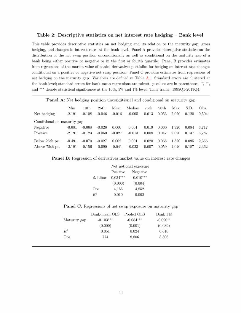
Table 2: Descriptive statistics on net interest rate hedging – Bank level
This table provides descriptive statistics on net hedging and its relation to the maturity gap, grosshedging, and changes in interest rates at the bank level. Panel A provides descriptive statistics on thedistribution of the net swap position unconditionally as well as conditional on the maturity gap of abank being either positive or negative or in the first or fourth quartile. Panel B provides estimatesfrom regressions of the market value of banks’ derivatives portfolios for hedging on interest rate changesconditional on a positive or negative net swap position. Panel C provides estimates from regressions ofnet hedging on the maturity gap. Variables are defined in Table A1. Standard errors are clustered atthe bank level; standard errors for bank-mean regressions are robust. p-values are in parentheses. ∗, ∗∗,and ∗∗∗ denote statistical significance at the 10%, 5% and 1% level. Time frame: 1995Q1-2013Q4.
Panel A: Net hedging position unconditional and conditional on maturity gap
Min 10th 25th Mean Median 75th 90th Max S.D. Obs.Net hedging -2.191 -0.108 -0.046 -0.016 -0.005 0.013 0.053 2.020 0.120 9,504
Conditional on maturity gapNegative -0.681 -0.068 -0.026 0.000 0.001 0.019 0.060 1.320 0.084 3,717Positive -2.191 -0.123 -0.060 -0.027 -0.013 0.008 0.047 2.020 0.137 5,787
Below 25th pc. -0.491 -0.070 -0.027 0.002 0.001 0.020 0.065 1.320 0.095 2,356Above 75th pc. -2.191 -0.156 -0.090 -0.041 -0.023 0.007 0.059 2.020 0.187 2,362
Panel B: Regression of derivatives market value on interest rate changes
Net notional exposurePositive Negative
∆ Libor 0.034∗∗∗ -0.010∗∗∗
(0.000) (0.004)Obs. 4,155 4,852R2 0.010 0.002
Panel C: Regressions of net swap exposure on maturity gap
Bank-mean OLS Pooled OLS Bank FEMaturity gap -0.103∗∗∗ -0.084∗∗∗ -0.090∗∗
(0.000) (0.001) (0.039)R2 0.051 0.024 0.010Obs. 774 8,806 8,806
41

Table 3: Cross-sectional evidence on hedging and net worth – BHC level
This table provides evidence on the relation between gross hedging and our measures of net worth at theBHC level. Panel A provides estimates from BHC-mean OLS and pooled OLS (with time fixed effects)specifications, including observations for which hedging equals zero. Panel B provides estimates from thefollowing specifications: BHC-mean Tobit, pooled Tobit (with time fixed effects), quantile regressionsat the 75th, 85th, and 95th percentile, and the second stage of a Heckman selection model using thenet worth index and, in the first stage, also size as explanatory variables. Panel C provides estimatesfrom specifications with credit rating dummies; credit ratings of A- and above are excluded. Variablesare defined in Table A1. Standard errors are clustered at the BHC level; standard errors for BHC-meanregressions are robust. p-values are in parentheses. ∗, ∗∗, and ∗∗∗ denote statistical significance at the10%, 5% and 1% level. Time frame: 1995Q1-2013Q4.
Model Size Mkt. cap. Mkt. cap./ Net Div. Rating Net worthAssets income index
Panel A: OLS regressions
BHC-mean 0.034∗∗∗ 0.025∗∗∗ 0.060 0.962∗∗∗ 15.884∗∗∗ 0.014∗∗ 0.014∗∗∗
OLS (0.000) (0.000) (0.313) (0.000) (0.004) (0.033) (0.000)
Pooled OLS 0.031∗∗∗ 0.023∗∗∗ 0.017 0.344∗∗∗ 3.304∗∗∗ 0.013∗∗∗ 0.010∗∗∗
with time FE (0.000) (0.000) (0.143) (0.000) (0.000) (0.000) (0.000)
Panel B: Tobit, quantile regressions, and Heckman model
BHC-mean 0.052∗∗∗ 0.040∗∗∗ -0.059 0.681∗ 17.631∗∗∗ 0.013∗∗ 0.018∗∗∗
Tobit (0.000) (0.000) (0.426) (0.098) (0.005) (0.010) (0.000)
Tobit 0.055∗∗∗ 0.043∗∗∗ 0.130∗∗∗ 0.695∗∗∗ 11.958∗∗∗ 0.014∗∗∗ 0.022∗∗∗
with time FE (0.000) (0.000) (0.000) (0.000) (0.000) (0.000) (0.000)
Quantile regres- 0.031∗∗∗ 0.019∗∗∗ 0.112∗∗∗ 0.338∗∗∗ 16.142∗∗∗ 0.016∗∗∗ 0.008∗∗∗
sion 75th pctile (0.000) (0.000) (0.000) (0.000) (0.000) (0.000) (0.000)
Quantile regres- 0.049∗∗∗ 0.029∗∗∗ 0.131∗∗∗ 0.599∗∗∗ 22.791∗∗∗ 0.021∗∗∗ 0.014∗∗∗
sion 85th pctile (0.000) (0.000) (0.000) (0.000) (0.000) (0.000) (0.000)
Quantile regres- 0.086∗∗∗ 0.053∗∗∗ 0.096 1.208∗∗∗ 29.678∗∗∗ 0.050∗∗∗ 0.026∗∗∗
sion 95th pctile (0.000) (0.000) (0.146) (0.000) (0.000) (0.000) (0.000)
Heckman selec- 0.005∗∗∗
tion model (0.000)
Panel C: Rating dummies
Pooled OLS BHC FEBBB- to BBB+ -0.078∗∗∗ 0.009∗∗∗
BB- to BB+ -0.053∗∗∗ 0.024∗∗∗
B- to B+ -0.124∗∗∗ -0.043∗∗∗
CCC+ and below -0.153∗∗∗ -0.132∗∗∗
42
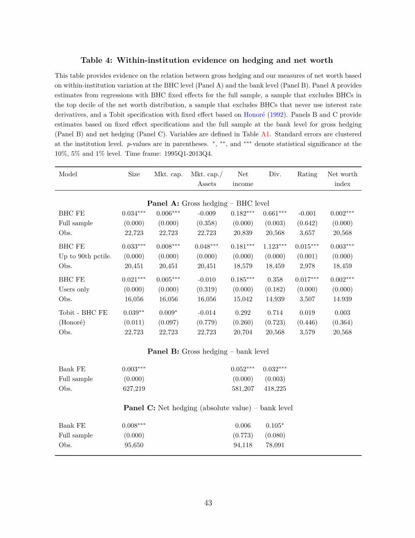
Table 4: Within-institution evidence on hedging and net worth
This table provides evidence on the relation between gross hedging and our measures of net worth basedon within-institution variation at the BHC level (Panel A) and the bank level (Panel B). Panel A providesestimates from regressions with BHC fixed effects for the full sample, a sample that excludes BHCs inthe top decile of the net worth distribution, a sample that excludes BHCs that never use interest ratederivatives, and a Tobit specification with fixed effect based on Honoré (1992). Panels B and C provideestimates based on fixed effect specifications and the full sample at the bank level for gross hedging(Panel B) and net hedging (Panel C). Variables are defined in Table A1. Standard errors are clusteredat the institution level. p-values are in parentheses. ∗, ∗∗, and ∗∗∗ denote statistical significance at the10%, 5% and 1% level. Time frame: 1995Q1-2013Q4.
Model Size Mkt. cap. Mkt. cap./ Net Div. Rating Net worthAssets income index
Panel A: Gross hedging – BHC levelBHC FE 0.034∗∗∗ 0.006∗∗∗ -0.009 0.182∗∗∗ 0.661∗∗∗ -0.001 0.002∗∗∗
Full sample (0.000) (0.000) (0.358) (0.000) (0.003) (0.642) (0.000)Obs. 22,723 22,723 22,723 20,839 20,568 3,657 20,568
BHC FE 0.033∗∗∗ 0.008∗∗∗ 0.048∗∗∗ 0.181∗∗∗ 1.123∗∗∗ 0.015∗∗∗ 0.003∗∗∗
Up to 90th pctile. (0.000) (0.000) (0.000) (0.000) (0.000) (0.001) (0.000)Obs. 20,451 20,451 20,451 18,579 18,459 2,978 18,459
BHC FE 0.021∗∗∗ 0.005∗∗∗ -0.010 0.185∗∗∗ 0.358 0.017∗∗∗ 0.002∗∗∗
Users only (0.000) (0.000) (0.319) (0.000) (0.182) (0.000) (0.000)Obs. 16,056 16,056 16,056 15,042 14,939 3,507 14.939
Tobit - BHC FE 0.039∗∗ 0.009∗ -0.014 0.292 0.714 0.019 0.003(Honoré) (0.011) (0.097) (0.779) (0.260) (0.723) (0.446) (0.364)Obs. 22,723 22,723 22,723 20,704 20,568 3,579 20,568
Panel B: Gross hedging – bank level
Bank FE 0.003∗∗∗ 0.052∗∗∗ 0.032∗∗∗
Full sample (0.000) (0.000) (0.003)Obs. 627,219 581,207 418,225
Panel C: Net hedging (absolute value) – bank level
Bank FE 0.008∗∗∗ 0.006 0.105∗
Full sample (0.000) (0.773) (0.080)Obs. 95,650 94,118 78,091
43

Table 5: Hedging before distress
This table provides evidence on hedging before distress. The table provides estimates from regressions ofhedging on dummies for up to 8 quarters before distress at the BHC and bank level. Distress events aredefined as exits from the sample with a ratio of market capitalization (for BHCs) or equity (for banks)to total assets below 4%. The table provides estimates for gross hedging at the BHC level and gross andnet hedging at the bank level. Variables are defined in Table A1. Standard errors are clustered at theinstitution level. p-values are in parentheses. ∗, ∗∗, and ∗∗∗ denote statistical significance at the 10%, 5%and 1% level. Time frame: 1995Q1-2013Q4.
BHC level Bank levelEvent time Gross hedging p-value Gross hedging p-value Net hedging p-value
τ − 8 -0.007 (0.439) -0.002 (0.766) -0.003 (0.646)τ − 7 -0.011 (0.216) -0.000 (0.909) -0.002 (0.714)τ − 6 -0.013 (0.136) -0.006 (0.380) -0.007 (0.310)τ − 5 -0.020∗∗ (0.023) -0.013∗∗ (0.065) -0.006 (0.346)τ − 4 -0.020∗∗ (0.023) -0.014∗∗ (0.049) -0.007 (0.246)τ − 3 -0.021∗∗ (0.012) -0.013∗ (0.067) -0.011∗ (0.081)τ − 2 -0.020∗∗ (0.022) -0.012∗ (0.083) -0.010 (0.123)τ − 1 -0.026∗∗∗ (0.002) -0.018∗∗ (0.011) -0.019∗∗∗ (0.004)τ -0.026∗∗∗ (0.002) -0.023∗∗∗ (0.001) -0.019∗∗∗ (0.003)
Institution FE Yes Yes YesTime FE Yes Yes YesObs. 16,056 51,520 8,489No. distressed 49 636 358Within-R2 0.013 0.036 0.011
44
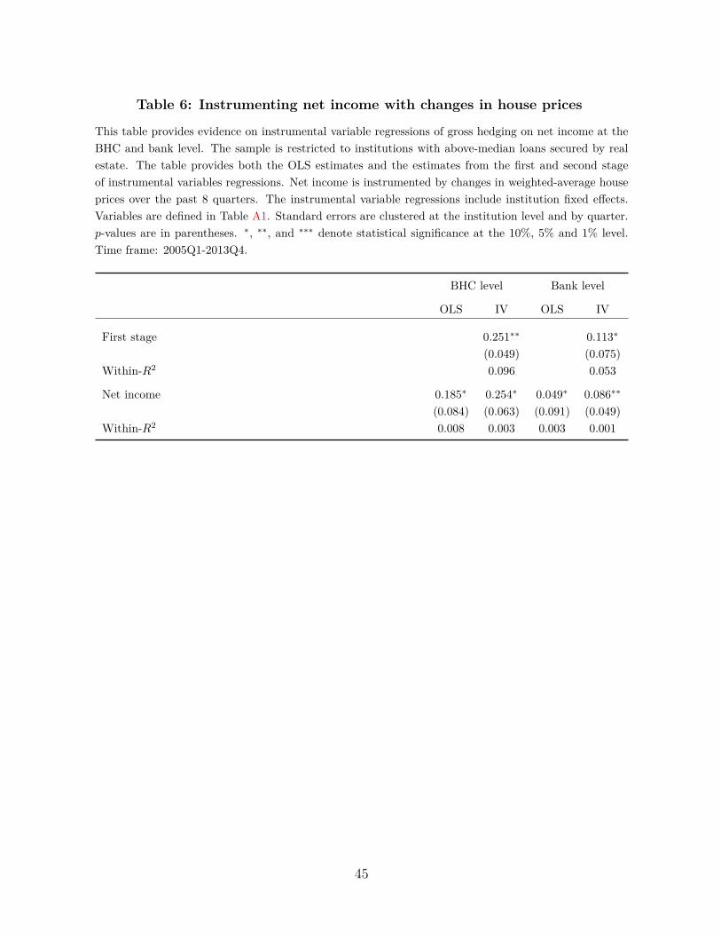
Table 6: Instrumenting net income with changes in house prices
This table provides evidence on instrumental variable regressions of gross hedging on net income at theBHC and bank level. The sample is restricted to institutions with above-median loans secured by realestate. The table provides both the OLS estimates and the estimates from the first and second stageof instrumental variables regressions. Net income is instrumented by changes in weighted-average houseprices over the past 8 quarters. The instrumental variable regressions include institution fixed effects.Variables are defined in Table A1. Standard errors are clustered at the institution level and by quarter.p-values are in parentheses. ∗, ∗∗, and ∗∗∗ denote statistical significance at the 10%, 5% and 1% level.Time frame: 2005Q1-2013Q4.
BHC level Bank level
OLS IV OLS IV
First stage 0.251∗∗ 0.113∗
(0.049) (0.075)Within-R2 0.096 0.053
Net income 0.185∗ 0.254∗ 0.049∗ 0.086∗∗
(0.084) (0.063) (0.091) (0.049)Within-R2 0.008 0.003 0.003 0.001
45

Table 7: Effect of net worth on hedging – Difference-in-differences estimates
This table provides the difference-in-differences estimates at the BHC level (Panel A) and the banklevel (Panel B) for three specifications of the treatment. The dependent variable is gross hedging. Thetreatment group is defined as the bottom 30% and the control group at the top 30% of institutions in2009 in terms of net income (Columns (1) to (3)), deposit weighted-average ZIP code level house pricechanges in 2007Q1 through 2008Q4 (Columns (4) to (6)), and deposit weighted-average MSA level Saiz(2010) housing supply elasticity in 2008Q4 (Columns (7) to (9)). We restrict the sample to institutionswith above-median loans secured by real estate to total assets in 2008Q4. In both panels, the sample isrestricted to institutions that hedge at least once before the treatment. Variables are defined in Table A1.Standard errors are clustered at the institution level. p-values are in parentheses. ∗, ∗∗, and ∗∗∗ denotestatistical significance at the 10%, 5% and 1% level. Time frame: 2005Q1-2013Q4.
Treatment Net income House price change Housing supply elasticity(1) (2) (3) (4) (5) (6) (7) (8) (9)
Post-event Year Year Post-event Year Year Post-event Year Yeardummy dummies dummies dummy dummies dummies dummy dummies dummies
Panel A: BHC level
2009 and -0.029∗∗ -0.040∗ -0.042∗
after (0.042) (0.056) (0.051)2009 -0.020 -0.022∗∗ -0.022 -0.026∗ -0.027∗∗ -0.096∗∗
(0.259) (0.025) (0.246) (0.098) (0.026) (0.037)2010 -0.039∗∗ -0.042∗∗∗ -0.022 -0.026 -0.027∗∗ -0.092∗∗
(0.026) (0.009) (0.154) (0.111) (0.035) (0.043)2011 -0.038∗∗ -0.035∗∗ -0.044∗ -0.051∗∗ -0.026∗∗ -0.059∗
(0.037) (0.046) (0.055) (0.049) (0.041) (0.056)2012 -0.019 -0.020∗ -0.042∗ -0.039∗ -0.021∗ -0.055∗
(0.263) (0.089) (0.065) (0.085) (0.054) (0.062)2013 -0.031∗ -0.033∗ -0.025 -0.016 -0.019∗ -0.047
(0.099) (0.053) (0.147) (0.326) (0.096) (0.112)BHC FE No No Yes No No Yes No No YesTime FE Yes Yes Yes Yes Yes Yes Yes Yes Yes
Panel B: Bank level
2009 and -0.015∗∗∗ -0.018∗ -0.005after (0.009) (0.068) (0.345)2009 -0.019∗∗ -0.017∗∗ -0.014∗ -0.018∗ -0.002 -0.003
(0.042) (0.031) (0.094) (0.087) (0.756) (0.621)2010 -0.010 -0.017∗∗ -0.014∗ -0.018∗ -0.002 -0.003
(0.181) (0.019) (0.094) (0.087) (0.756) (0.621)2011 0.001 0.006 -0.022∗ -0.025∗ -0.004 -0.003
(0.910) (0.390) (0.056) (0.064) (0.458) (0.352)2012 -0.021∗∗∗ -0.027∗∗∗ -0.019 -0.021 -0.010 -0.006
(0.008) (0.000) (0.125) (0.100) (0.555) (0.489)2013 −0.028∗∗∗ -0.018∗∗ -0.008 -0.010 0.002 0.014
(0.000) (0.017) (0.341) (0.239) (0.672) (0.534)Bank FE No No Yes No No Yes No No YesTime FE Yes Yes Yes Yes Yes Yes Yes Yes Yes
46

Table 8: Robustness – Pre-treatment differences and effect on maturity gap
This table provides two sets of robustness estimates comparing the treatment and control groups usingnet income to define the treatment variable as in columns (1) to (3) in Table 7. Panel A provides estimatesfrom a difference-in-differences specification at the BHC level as in columns (1) to (3) in Panel A of Table 7but includes treatment-dummies for the pre-treatment period as well. Panel B provides estimates froma difference-in-differences specification using the maturity gap as the dependent variable using data atboth the BHC and bank level, and the duration gap at the bank level. In both panels, the sample isrestricted to institutions that hedge at least once before the treatment. Variables are defined in Table A1.Standard errors are clustered at the institution level. p-values are in parentheses. ∗, ∗∗, and ∗∗∗ denotestatistical significance at the 10%, 5% and 1% level. Time frame: 2005Q1-2013Q4.
Panel A: Difference-in-difference estimates with pre-treatment year dummies
Year Yeardummies dummies
2005 -0.014 (0.331) -0.003 (0.784)2006 -0.010 (0.499) 0.008 (0.444)2007 -0.007 (0.626) -0.000 (0.989)2008 – –2009 -0.028∗ (0.085) -0.017 (0.134)2010 -0.047∗∗∗ (0.004) -0.029∗∗ (0.010)2011 -0.046∗∗∗ (0.005) -0.028∗∗ (0.015)2012 -0.027∗ (0.095) -0.030∗∗∗ (0.009)2013 -0.039∗∗ (0.019) -0.036∗∗∗ (0.002)
BHC FE No YesTime FE Yes Yes
Panel B: Effect of treatment on maturity gap
BHC level Bank level
Maturity gap Maturity gap Duration gap2009 and after -0.025 -0.038 -0.037
(0.352) (0.232) (0.920)2009 -0.087∗∗ -0.094∗∗∗ -0.027
(0.021) (0.012) (0.932)2010 -0.019 -0.036 0.025
(0.609) (0.303) (0.965)2011 -0.021 -0.041 0.039
(0.569) (0.204) (0.946)2012 0.008 -0.006 0.034
(0.817) (0.862) (0.958)2013 -0.008 -0.014 0.042
(0.815) (0.663) (0.924)Institution FE and Time FE Yes Yes Yes Yes Yes Yes
47
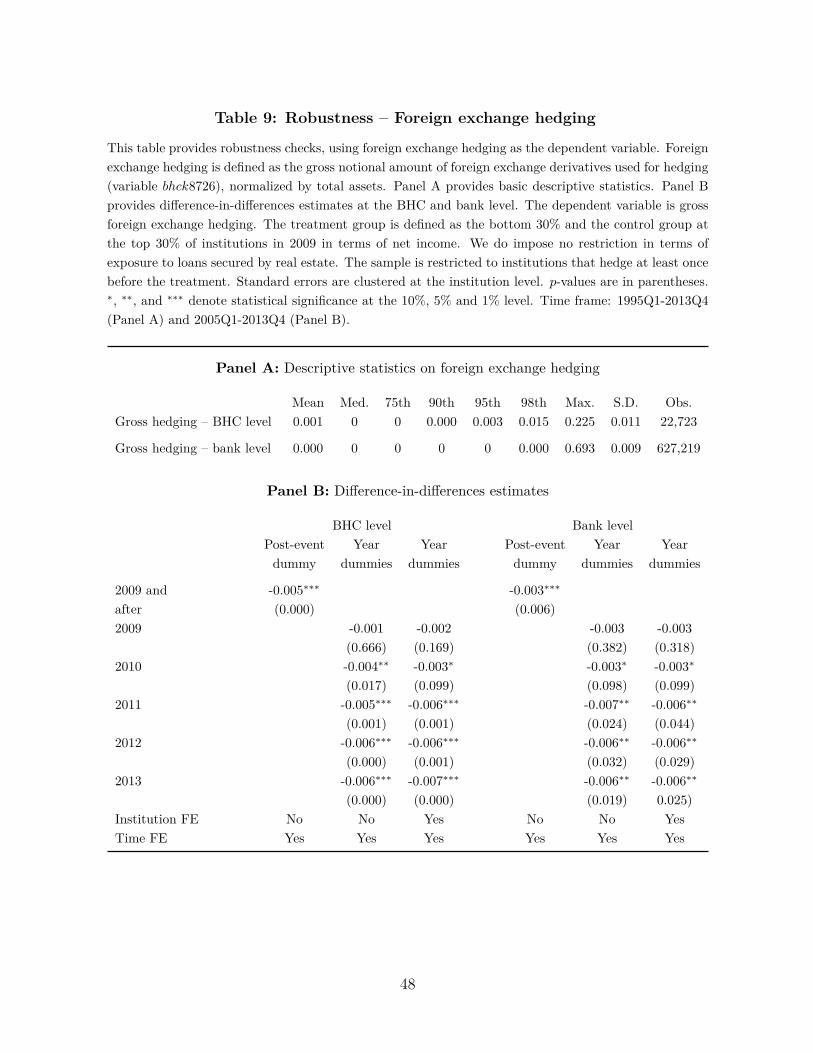
Table 9: Robustness – Foreign exchange hedging
This table provides robustness checks, using foreign exchange hedging as the dependent variable. Foreignexchange hedging is defined as the gross notional amount of foreign exchange derivatives used for hedging(variable bhck8726), normalized by total assets. Panel A provides basic descriptive statistics. Panel Bprovides difference-in-differences estimates at the BHC and bank level. The dependent variable is grossforeign exchange hedging. The treatment group is defined as the bottom 30% and the control group atthe top 30% of institutions in 2009 in terms of net income. We do impose no restriction in terms ofexposure to loans secured by real estate. The sample is restricted to institutions that hedge at least oncebefore the treatment. Standard errors are clustered at the institution level. p-values are in parentheses.∗, ∗∗, and ∗∗∗ denote statistical significance at the 10%, 5% and 1% level. Time frame: 1995Q1-2013Q4(Panel A) and 2005Q1-2013Q4 (Panel B).
Panel A: Descriptive statistics on foreign exchange hedging
Mean Med. 75th 90th 95th 98th Max. S.D. Obs.Gross hedging – BHC level 0.001 0 0 0.000 0.003 0.015 0.225 0.011 22,723
Gross hedging – bank level 0.000 0 0 0 0 0.000 0.693 0.009 627,219
Panel B: Difference-in-differences estimates
BHC level Bank levelPost-event Year Year Post-event Year Yeardummy dummies dummies dummy dummies dummies
2009 and -0.005∗∗∗ -0.003∗∗∗
after (0.000) (0.006)2009 -0.001 -0.002 -0.003 -0.003
(0.666) (0.169) (0.382) (0.318)2010 -0.004∗∗ -0.003∗ -0.003∗ -0.003∗
(0.017) (0.099) (0.098) (0.099)2011 -0.005∗∗∗ -0.006∗∗∗ -0.007∗∗ -0.006∗∗
(0.001) (0.001) (0.024) (0.044)2012 -0.006∗∗∗ -0.006∗∗∗ -0.006∗∗ -0.006∗∗
(0.000) (0.001) (0.032) (0.029)2013 -0.006∗∗∗ -0.007∗∗∗ -0.006∗∗ -0.006∗∗
(0.000) (0.000) (0.019) 0.025)Institution FE No No Yes No No YesTime FE Yes Yes Yes Yes Yes Yes
48

Table 10: Derivatives trading and net worth
This table provides evidence on the relation between trading and net worth. Trading is measured asgross derivatives positions held for trading normalized by total assets. Panel A provides estimates fromregressions of trading on our measures of net worth at the BHC level from three specifications: a BHC-mean Tobit, a Tobit with time fixed effects, and a regression with BHC fixed effects. Panel B providesestimates from regressions of trading on dummies for up to 8 quarters before distress at the BHC andbank level. Variables are defined in Table A1. Standard errors are clustered at the institution level;standard errors for BHC-mean regressions are robust. p-values are in parentheses. ∗, ∗∗, and ∗∗∗ denotestatistical significance at the 10%, 5% and 1% level. Time frame: 1995Q1-2013Q4.
Panel A: OLS and fixed effect regressions
Model Size Mkt. cap. Mkt. cap./ Net Div. Rating Net worthAssets income index
BHC-mean 0.579∗∗∗ 0.484∗∗∗ 0.600 9.361∗ 374.661∗∗∗ 0.872∗∗∗ 0.303∗∗∗
Tobit (0.000) (0.000) (0.509) (0.089) (0.000) (0.000) (0.000)R2 0.267 0.215 0.000 0.001 0.011 0.036 0.036
Tobit 0.590∗∗∗ 0.511∗∗∗ 3.300∗∗∗ 11.459∗∗∗ 164.830∗∗∗ 0.809∗∗∗ 0.358∗∗∗
with time FE (0.000) (0.000) (0.000) (0.000) (0.000) (0.000) (0.000)R2 0.318 0.279 0.014 0.009 0.012 0.045 0.063
BHC FE 0.082∗∗∗ 0.020∗∗∗ 0.692∗∗∗ 1.172∗∗∗ 5.965 0.040 0.096∗∗
(0.000) (0.010) (0.000) (0.001) (0.471) (0.127) (0.024)Within-R2 0.009 0.042 0.049 0.044 0.042 0.096 0.134
Panel B: Derivatives trading before distress
BHC level Bank levelEvent time Gross trading p-value Gross trading p-valueτ − 8 -0.020 (0.458) 0.009 (0.417)τ − 7 -0.045∗∗∗ (0.002) 0.011 (0.396)τ − 6 -0.038∗∗∗ (0.009) 0.012 (0.357)τ − 5 -0.042∗∗∗ (0.009) 0.020 (0.491)τ − 4 -0.041∗∗ (0.014) 0.014 (0.457)τ − 3 -0.053∗∗∗ (0.006) 0.009 (0.544)τ − 2 -0.052∗∗∗ (0.005) 0.012 (0.250)τ − 1 -0.053∗∗ (0.010) 0.013 (0.241)τ -0.059∗∗∗ (0.003) 0.006 (0.599)
Institution FE Yes YesTime FE Yes YesObs. 5,955 18,540No. distressed 10 224Within-R2 0.042 0.005
49
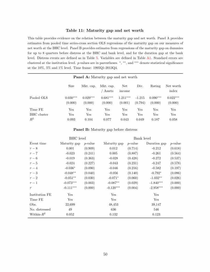
Table 11: Maturity gap and net worth
This table provides evidence on the relation between the maturity gap and net worth. Panel A providesestimates from pooled time series-cross section OLS regressions of the maturity gap on our measures ofnet worth at the BHC level. Panel B provides estimates from regressions of the maturity gap on dummiesfor up to 8 quarters before distress at the BHC and bank level, and for the duration gap at the banklevel. Distress events are defined as in Table 5. Variables are defined in Table A1. Standard errors areclustered at the institution level. p-values are in parentheses. ∗, ∗∗, and ∗∗∗ denote statistical significanceat the 10%, 5% and 1% level. Time frame: 1995Q1-2013Q4.
Panel A: Maturity gap and net worth
Size Mkt. cap. Mkt. cap. Net Div. Rating Net worth/ Assets income index
Pooled OLS 0.030∗∗∗ 0.029∗∗∗ 0.681∗∗∗ 1.211∗∗∗ -1.215 0.090∗∗∗ 0.022∗∗∗
(0.000) (0.000) (0.000) (0.001) (0.794) (0.000) (0.000)
Time FE Yes Yes Yes Yes Yes Yes YesBHC cluster Yes Yes Yes Yes Yes Yes YesR2 0.093 0.104 0.077 0.043 0.049 0.187 0.058
Panel B: Maturity gap before distress
BHC level Bank levelEvent time Maturity gap p-value Maturity gap p-value Duration gap p-valueτ − 8 0.001 (0.909) 0.012 (0.714) -0.212 (0.618)τ − 7 -0.023 (0.241) 0.005 (0.887) -0.261 (0.564)τ − 6 -0.019 (0.363) -0.028 (0.428) -0.272 (0.537)τ − 5 -0.024 (0.227) -0.043 (0.231) -0.247 (0.578)τ − 4 -0.036∗ (0.090) -0.046 (0.216) -0.582 (0.197)τ − 3 -0.048∗∗ (0.040) -0.056 (0.140) -0.792∗ (0.086)τ − 2 -0.051∗∗ (0.030) -0.071∗ (0.060) -1.032∗∗ (0.026)τ − 1 -0.073∗∗∗ (0.003) -0.087∗∗ (0.029) -1.840∗∗∗ (0.000)τ -0.111∗∗∗ (0.000) -0.120∗∗∗ (0.004) -2.958∗∗∗ (0.000)
Institution FE Yes Yes YesTime FE Yes Yes YesObs. 22,699 48,453 39,147No. distressed 49 636 546Within-R2 0.052 0.132 0.123
50

Figure 1: Net hedging conditional on maturity gap – Bank level
This figure shows the distribution of the net hedging position of banks in the first and fourth quartilesof the maturity gap distribution. Variables are defined in Table A1.
−0.2 −0.15 −0.1 −0.05 0 0.05 0.1 0.15 0.20
0.02
0.04
0.06
0.08
0.1
0.12
0.14
0.16
0.18
0.2
Den
sity
Net hedging
Maturity gap > 75th percentile
Maturity gap < 25th percentile
51
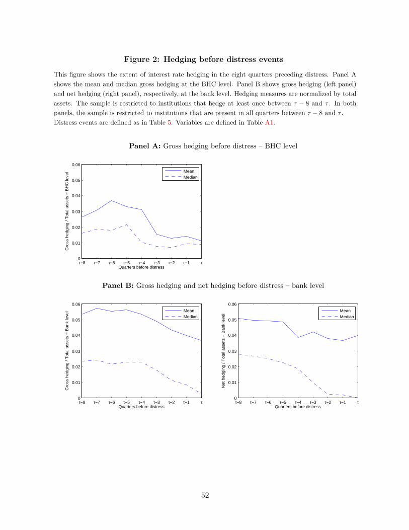
Figure 2: Hedging before distress events
This figure shows the extent of interest rate hedging in the eight quarters preceding distress. Panel Ashows the mean and median gross hedging at the BHC level. Panel B shows gross hedging (left panel)and net hedging (right panel), respectively, at the bank level. Hedging measures are normalized by totalassets. The sample is restricted to institutions that hedge at least once between τ − 8 and τ . In bothpanels, the sample is restricted to institutions that are present in all quarters between τ − 8 and τ .Distress events are defined as in Table 5. Variables are defined in Table A1.
Panel A: Gross hedging before distress – BHC level
0
0.01
0.02
0.03
0.04
0.05
0.06
τ−8 τ−7 τ−6 τ−5 τ−4 τ−3 τ−2 τ−1 τ Quarters before distress
Gro
ss h
edgi
ng /
Tot
al a
sset
s −
BH
C le
vel
MeanMedian
Panel B: Gross hedging and net hedging before distress – bank level
0
0.01
0.02
0.03
0.04
0.05
0.06
τ−8 τ−7 τ−6 τ−5 τ−4 τ−3 τ−2 τ−1 τ Quarters before distress
Gro
ss h
edgi
ng /
Tot
al a
sset
s −
Ban
k le
vel
MeanMedian
0
0.01
0.02
0.03
0.04
0.05
0.06
τ−8 τ−7 τ−6 τ−5 τ−4 τ−3 τ−2 τ−1 τ Quarters before distress
Net
hed
ging
/ T
otal
ass
ets
− B
ank
leve
l
MeanMedian
52
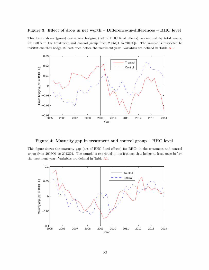
Figure 3: Effect of drop in net worth – Difference-in-differences – BHC level
This figure shows (gross) derivatives hedging (net of BHC fixed effects), normalized by total assets,for BHCs in the treatment and control group from 2005Q1 to 2013Q4. The sample is restricted toinstitutions that hedge at least once before the treatment year. Variables are defined in Table A1.
2005 2006 2007 2008 2009 2010 2011 2012 2013 2014−0.03
−0.02
−0.01
0
0.01
0.02
0.03
Year
Gro
ss h
edgi
ng (
net o
f BH
C F
E)
Treated
Control
Figure 4: Maturity gap in treatment and control group – BHC level
This figure shows the maturity gap (net of BHC fixed effects) for BHCs in the treatment and controlgroup from 2005Q1 to 2013Q4. The sample is restricted to institutions that hedge at least once beforethe treatment year. Variables are defined in Table A1.
2005 2006 2007 2008 2009 2010 2011 2012 2013 2014−0.1
−0.05
0
0.05
0.1
Year
Mat
urity
gap
(ne
t of B
HC
FE
)
Treated
Control
53

Figure 5: Foreign exchange hedging – Difference-in-differences – BHC level
This figure shows (gross) foreign exchange hedging (net of BHC fixed effects), normalized by total assets,for BHCs in the treatment and control group from 2005Q1 to 2013Q4. The sample is restricted toinstitutions that hedge at least once before the treatment year. The foreign exchange hedging variableis defined in Table 9.
2005 2006 2007 2008 2009 2010 2011 2012 2013 2014−5
0
5x 10
−3
Year
For
eign
exc
hang
e he
dgin
g (n
et o
f BH
C F
E)
TreatedControl
54

Appendix – For Online Publication
Appendix A: Auxiliary tables and figures
Table A1: Variable definitions
This table provides the definitions of the variables used in the empirical analysis. In the call reports,variables for bank holding companies (BHCs) and banks are reported with different prefixes, bhck forBHCs and rcon or rcfd for banks. When a variable is similar for BHCs and banks, its suffix is the same.For example, total assets are denoted bhck2170 for BHCs and rcon2170 for banks. When the samevariable exists for BHCs and banks, only the BHC-level variable is reported in our definition.
Variable Definition Data source
Derivatives data
Gross hedging Total gross notional amount of interest rate derivative con-tracts held for purposes other than trading (bhck8725 ) overtotal assets; for the period 1995-2000, contracts not markedto market (bhck8729 ) are added; winsorized at the 99thpercentile
Call reports
Net hedging Interest rate swaps where the bank has agreed to pay a fixedrate (rcona589 ) minus pay-float swaps (computed as totalswaps minus pay-fixed swaps), normalized by total assets;can be computed only for banks that report only swaps
Call reports
Gross trading Total gross notional amount of interest rate derivative con-tracts held for trading (bhcka126 )
Call reports
Net worth and regulatory capital
Size Log of total assets (bhck2170 ) Call reportsMarket capitalization Log of share mid-price at the end of each quarter, multiplied
by the number of shares outstandingCRSP
Market capitalization/ Assets
Market capitalization normalized by total assets (at bookvalue) minus book equity plus market capitalization; win-sorized at the 1st and 99th percentiles
CRSP
Net income / Assets Net income (bhck4340 ) normalized by total assets; win-sorized at the 1st and 99th percentiles
Call reports
Dividends / Assets Cash dividends on common stock (bhck4460 ); winsorizedat the 1st and 99th percentiles
Call reports
Credit rating Credit rating from Standard & Poors coded linearly from1 (D) to 22 (AAA)
Capital IQ
Net worth index First principal component of Size, Market capitalization /Assets, Dividends / Assets and Net income / Assets withloadings of 0.149, 0.307, 0.272 and 0.272, respectively
Call reportsand CRSP
1
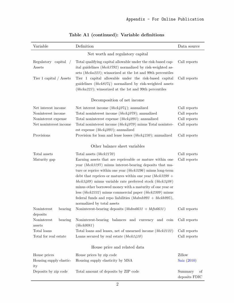
Appendix – For Online Publication
Table A1 (continued): Variable definitions
Variable Definition Data source
Net worth and regulatory capital
Regulatory capital /Assets
Total qualifying capital allowable under the risk-based cap-ital guidelines (bhck3792 ) normalized by risk-weighted as-sets (bhcka223 ); winsorized at the 1st and 99th percentiles
Call reports
Tier 1 capital / Assets Tier 1 capital allowable under the risk-based capitalguidelines (bhck8274 ) normalized by risk-weighted assets(bhcka223 ); winsorized at the 1st and 99th percentiles
Call reports
Decomposition of net income
Net interest income Net interest income (bhck4074 ); annualized Call reportsNoninterest income Total noninterest income (bhck4079 ); annualized Call reportsNoninterest expense Total noninterest expense (bhck4093 ); annualized Call reportsNet noninterest income Total noninterest income (bhck4079 ) minus Total noninter-
est expense (bhck4093 ); annualizedCall reports
Provisions Provision for loan and lease losses (bhck4230 ); annualized Call reports
Other balance sheet variables
Total assets Total assets (bhck2170 ) Call reportsMaturity gap Earning assets that are repriceable or mature within one
year (bhck3197 ) minus interest-bearing deposits that ma-ture or reprice within one year (bhck3296 ) minus long-termdebt that reprices or matures within one year (bhck3298 +bhck3409 ) minus variable rate preferred stock (bhck3408 )minus other borrowed money with a maturity of one year orless (bhck2332 ) minus commercial paper (bhck2309 ) minusfederal funds and repo liabilities (bhdmb993 + bhckb995 ),normalized by total assets
Call reports
Noninterest bearingdeposits
Noninterest-bearing deposits (bhdm6631 + bhfn6631 ) Call reports
Noninterest bearingassets
Noninterest-bearing balances and currency and coin(bhck0081 )
Call reports
Total loans Total loans and leases, net of unearned income (bhck2122 ) Call reportsTotal for real estate Loans secured by real estate (bhck1410 ) Call reports
House price and related data
House prices House prices by zip code ZillowHousing supply elastic-ity
Housing supply elasticity by MSA Saiz (2010)
Deposits by zip code Total amount of deposits by ZIP code Summary ofdeposits FDIC
2
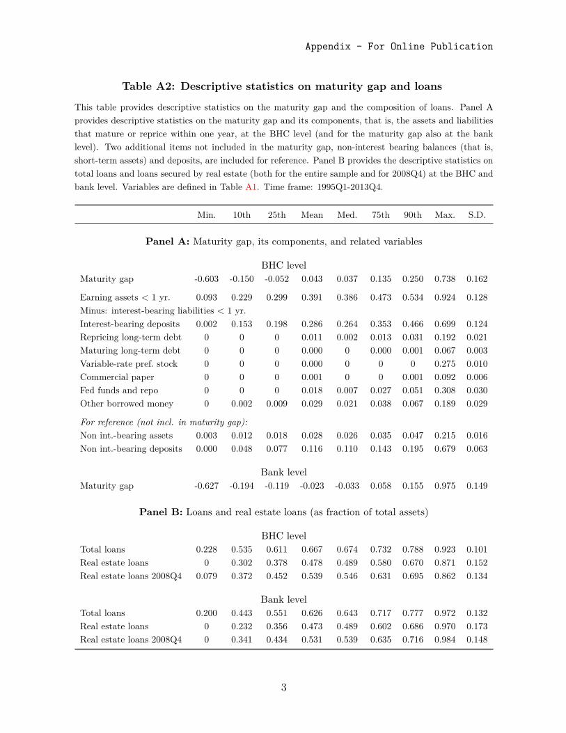
Appendix – For Online Publication
Table A2: Descriptive statistics on maturity gap and loans
This table provides descriptive statistics on the maturity gap and the composition of loans. Panel Aprovides descriptive statistics on the maturity gap and its components, that is, the assets and liabilitiesthat mature or reprice within one year, at the BHC level (and for the maturity gap also at the banklevel). Two additional items not included in the maturity gap, non-interest bearing balances (that is,short-term assets) and deposits, are included for reference. Panel B provides the descriptive statistics ontotal loans and loans secured by real estate (both for the entire sample and for 2008Q4) at the BHC andbank level. Variables are defined in Table A1. Time frame: 1995Q1-2013Q4.
Min. 10th 25th Mean Med. 75th 90th Max. S.D.
Panel A: Maturity gap, its components, and related variables
BHC levelMaturity gap -0.603 -0.150 -0.052 0.043 0.037 0.135 0.250 0.738 0.162
Earning assets < 1 yr. 0.093 0.229 0.299 0.391 0.386 0.473 0.534 0.924 0.128Minus: interest-bearing liabilities < 1 yr.Interest-bearing deposits 0.002 0.153 0.198 0.286 0.264 0.353 0.466 0.699 0.124Repricing long-term debt 0 0 0 0.011 0.002 0.013 0.031 0.192 0.021Maturing long-term debt 0 0 0 0.000 0 0.000 0.001 0.067 0.003Variable-rate pref. stock 0 0 0 0.000 0 0 0 0.275 0.010Commercial paper 0 0 0 0.001 0 0 0.001 0.092 0.006Fed funds and repo 0 0 0 0.018 0.007 0.027 0.051 0.308 0.030Other borrowed money 0 0.002 0.009 0.029 0.021 0.038 0.067 0.189 0.029
For reference (not incl. in maturity gap):Non int.-bearing assets 0.003 0.012 0.018 0.028 0.026 0.035 0.047 0.215 0.016Non int.-bearing deposits 0.000 0.048 0.077 0.116 0.110 0.143 0.195 0.679 0.063
Bank levelMaturity gap -0.627 -0.194 -0.119 -0.023 -0.033 0.058 0.155 0.975 0.149
Panel B: Loans and real estate loans (as fraction of total assets)
BHC levelTotal loans 0.228 0.535 0.611 0.667 0.674 0.732 0.788 0.923 0.101Real estate loans 0 0.302 0.378 0.478 0.489 0.580 0.670 0.871 0.152Real estate loans 2008Q4 0.079 0.372 0.452 0.539 0.546 0.631 0.695 0.862 0.134
Bank levelTotal loans 0.200 0.443 0.551 0.626 0.643 0.717 0.777 0.972 0.132Real estate loans 0 0.232 0.356 0.473 0.489 0.602 0.686 0.970 0.173Real estate loans 2008Q4 0 0.341 0.434 0.531 0.539 0.635 0.716 0.984 0.148
3
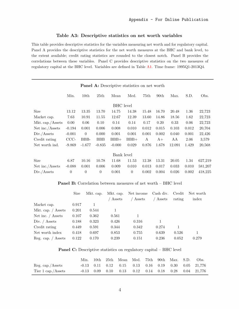
Appendix – For Online Publication
Table A3: Descriptive statistics on net worth variables
This table provides descriptive statistics for the variables measuring net worth and for regulatory capital.Panel A provides the descriptive statistics for the net worth measures at the BHC and bank level, tothe extent available; credit rating statistics are rounded to the closest notch. Panel B provides thecorrelations between these variables. Panel C provides descriptive statistics on the two measures ofregulatory capital at the BHC level. Variables are defined in Table A1. Time frame: 1995Q1-2013Q4.
Panel A: Descriptive statistics on net worth
Min. 10th 25th Mean Med. 75th 90th Max. S.D. Obs.
BHC levelSize 13.12 13.35 13.70 14.75 14.38 15.48 16.70 20.48 1.36 22,723Market cap. 7.63 10.91 11.55 12.67 12.39 13.60 14.86 18.56 1.62 22,723Mkt. cap./Assets 0.00 0.06 0.10 0.14 0.14 0.17 0.20 0.33 0.06 22,723Net inc./Assets -0.194 0.001 0.006 0.008 0.010 0.012 0.015 0.103 0.012 20,704Div./Assets -0.001 0 0.000 0.001 0.001 0.001 0.002 0.040 0.001 22,426Credit rating CCC- BBB- BBB BBB+ BBB+ A A+ AA 2.06 3,579Net worth ind. -9.869 -1.677 -0.835 -0.000 0.029 0.876 1.678 12.091 1.429 20,568
Bank levelSize 6.87 10.16 10.78 11.68 11.53 12.38 13.31 20.05 1.34 627,219Net inc./Assets -0.088 0.001 0.006 0.009 0.010 0.013 0.017 0.033 0.010 581,207Div./Assets 0 0 0 0.001 0 0.002 0.004 0.026 0.002 418,225
Panel B: Correlation between measures of net worth – BHC level
Size Mkt. cap. Mkt. cap. Net income Cash div. Credit Net worth/ Assets / Assets / Assets rating index
Market cap. 0.917 1Mkt. cap. / Assets 0.201 0.544 1Net inc. / Assets 0.107 0.362 0.561 1Div. / Assets 0.188 0.323 0.426 0.316 1Credit rating 0.449 0.591 0.344 0.342 0.274 1Net worth index 0.418 0.697 0.853 0.755 0.639 0.526 1Reg. cap. / Assets 0.122 0.170 0.239 0.151 0.236 0.052 0.279
Panel C: Descriptive statistics on regulatory capital – BHC level
Min. 10th 25th Mean Med. 75th 90th Max. S.D. Obs.Reg. cap./Assets -0.13 0.11 0.12 0.15 0.13 0.16 0.19 0.30 0.05 21,776Tier 1 cap./Assets -0.13 0.09 0.10 0.13 0.12 0.14 0.18 0.28 0.04 21,776
4

Appendix – For Online Publication
Table A4: Variance decomposition of net income – BHC level
This table provides a variance decomposition of net income at the BHC level. The table providesestimates from regressions of changes in net income on changes in various components of net income.Each column provides results from a separate regression. By definition, net income is the sum of threemain elements: Net interest income + Net noninterest income − Provisions, plus exceptional items whichare being neglected. Variables are defined in Table A1. Standard errors are clustered at the BHC level.t-statistics are in square brackets. Time frame: 2005Q1-2013Q4.
(1) (2) (3) (4) (5)
∆ Net interest income 0.736 0.091 0.760[19.05] [0.89] [18.57]
∆ Net noninterest income 0.904 0.967[34.94] [36.39]
∆ Noninterest income 0.807[22.31]
∆ Noninterest expense 0.918[34.45]
∆ Provisions -0.793 -1.045 -0.790[-34.34] [-21.63] [-33.42]
R2 0.803 0.000 0.605 0.307 0.804Obs 9,856 9,856 9,856 9,856 9,856
5

Appendix – For Online Publication
Table A5: Hedging and regulatory capital – BHC level
This table provides evidence on the relation between hedging and the regulatory capital of BHCs using thetwo measures of regulatory capital. Panel A reports estimates from BHC-mean OLS, pooled OLS, pooledTobit, and BHC fixed effect regressions of gross hedging on our measures of regulatory capital. Standarderrors are clustered at the BHC level; standard errors for BHC-mean regressions are robust. p-values arein parentheses. Panel B provides the results for the Davidson-MacKinnon J-tests of whether the modelswith our measures of regulatory capital and net worth are nested. The t-statistics are reported and p-values are in parentheses. Variables are defined in Table A1. ∗, ∗∗ and ∗∗∗ denote statistical significanceat the 10%, 5% and 1% level. Time frame: 1996Q1-2013Q4.
Panel A: Regression of hedging on regulatory capital
BHC-mean OLS Pooled OLS Pooled Tobit BHC FERegulatory cap. / Assets -0.224 0.260 0.192 0.113
(0.280) (0.114) (0.619) (0.318)R2 0.000 0.008 0.036 0.009
Tier 1 cap. / Assets 0.193 0.086 -0.337 0.247∗
(0.529) (0.472) (0.259) (0.060)R2 -0.000 0.008 0.036 0.009
Panel B: Davidson-MacKinnon (1981)’s J-test
Size Mkt. cap. Mkt. cap. Net Div. Rating Net worth/ Assets income index
Regulatory capital
H0: Reg. cap. /Assets 10.71∗∗∗ 9.93∗∗∗ 4.41∗∗∗ 3.59∗∗∗ 4.77∗∗∗ 3.85∗∗∗ 5.35∗∗∗
H1: Net worth explainsresiduals
(0.000) (0.000) (0.000) (0.000) (0.000) (0.000) (0.000)
H0: Net worth -0.70 -5.25∗∗∗ 1.48 -0.71 -0.33 5.62∗∗∗ -1.70∗
H1: Reg. cap./Assetsexplains residuals
(0.486) (0.000) (0.139) (0.479) (0.741) (0.000) (0.090)
Tier 1 capital
H0: Tier 1 cap. /Assets 10.71∗∗∗ 9.93∗∗∗ 4.41∗∗∗ 3.58∗∗∗ 4.76∗∗∗ 3.86∗∗∗ 5.60∗∗∗
H1: Net worth explainsresiduals
(0.000) (0.000) (0.000) (0.000) (0.000) (0.000) (0.000)
H0: Net worth -1.59 -3.53∗∗∗ 0.47 0.92 -1.67∗ -1.44 4.53∗∗∗
H1: Tier 1 cap./Assetsexplains residuals
(0.112) (0.000) (0.636) (0.360) (0.096) (0.151) (0.000)
6
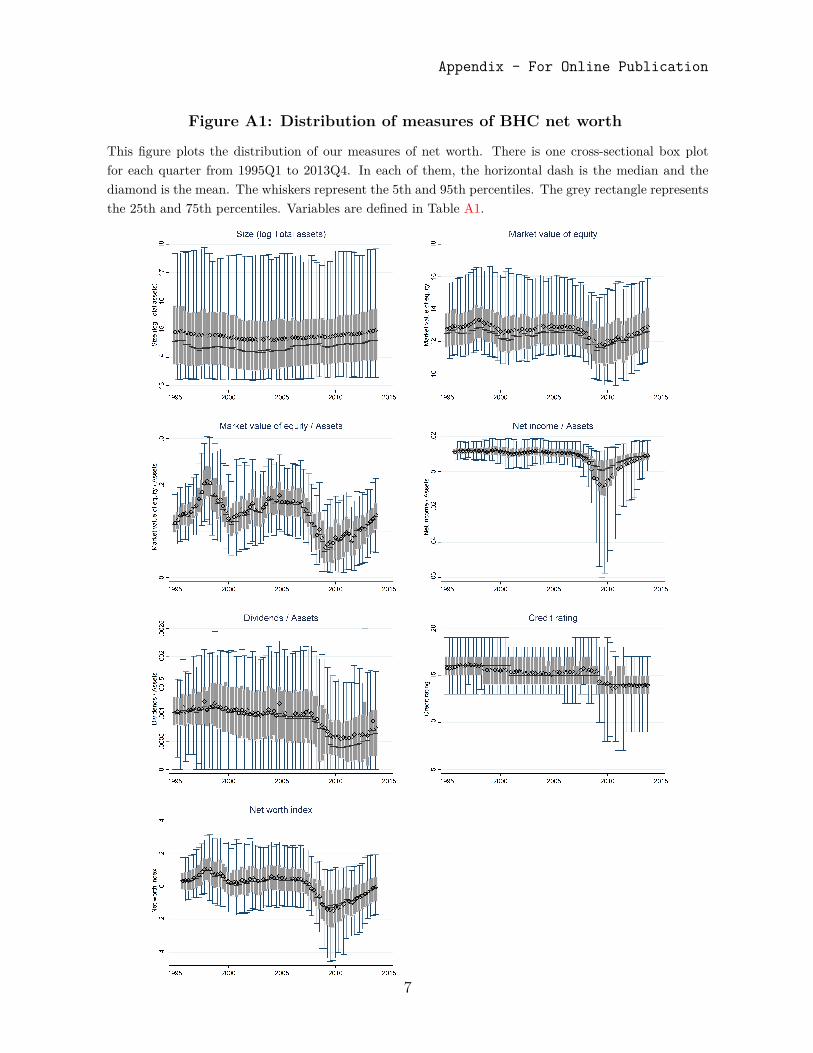
Appendix – For Online Publication
Figure A1: Distribution of measures of BHC net worth
This figure plots the distribution of our measures of net worth. There is one cross-sectional box plotfor each quarter from 1995Q1 to 2013Q4. In each of them, the horizontal dash is the median and thediamond is the mean. The whiskers represent the 5th and 95th percentiles. The grey rectangle representsthe 25th and 75th percentiles. Variables are defined in Table A1.
7
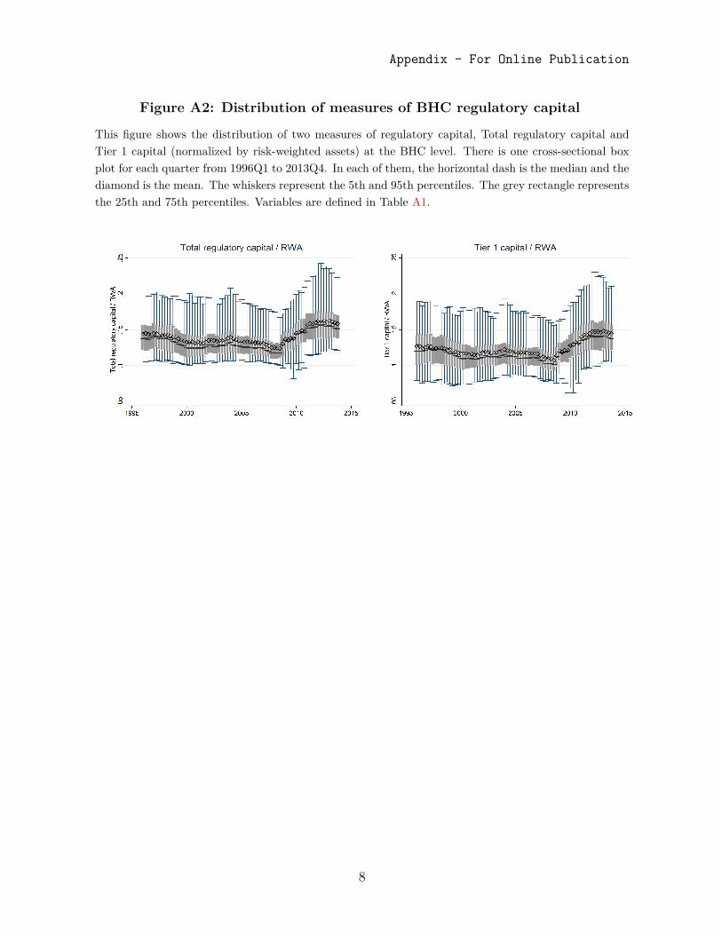
Appendix – For Online Publication
Figure A2: Distribution of measures of BHC regulatory capital
This figure shows the distribution of two measures of regulatory capital, Total regulatory capital andTier 1 capital (normalized by risk-weighted assets) at the BHC level. There is one cross-sectional boxplot for each quarter from 1996Q1 to 2013Q4. In each of them, the horizontal dash is the median and thediamond is the mean. The whiskers represent the 5th and 95th percentiles. The grey rectangle representsthe 25th and 75th percentiles. Variables are defined in Table A1.
8

Appendix – For Online Publication
Figure A3: Decomposition of net income – BHC level
This figure shows the distribution of BHCs’ net income and two key components of net income over theperiod from 1995Q1 to 2013Q4 in the top two panels and the bottom left panel. The top left panel showsthe distribution of net income (normalized by total assets); this panel also shows the year 2009 in darkred, which is the treatment year in our difference-in-differences estimation. The top right panel showsthe distribution of net interest income (normalized by total assets); the bottom left panel shows thedistribution of provisions for loan losses (normalized by total assets). The bottom right panel shows theratio of non-accrual loans to total assets, broken down by loan type. In the top two panels and bottomleft panel, there is one cross-sectional box plot for each quarter. In each of them, the horizontal dashis the median and the diamond is the mean. The whiskers represent the 5th and 95th percentiles. Thegrey rectangle represents the 25th and 75th percentiles. Variables are defined in Table A1.
1995 2000 2005 2010 20150
0.005
0.01
0.015
0.02
0.025
Year
Non
−ac
crua
l loa
ns /
Tot
al a
sset
s
Real−estate loans
Commercial loans
Other loans
9

Appendix – For Online Publication
Figure A4: Trading and maturity gap before distress events
This figure shows trading by banks and the maturity gap of BHCs and banks in the eight quarterspreceding distress. Panel A shows gross interest rate derivatives trading (normalized by total assets)at the bank level. The sample is restricted to banks that trade at least once between τ − 8 and τ .Panel B shows the maturity gap at the BHC and bank level. In both panels, the sample is restrictedto institutions that are present in all quarters between τ − 8 and τ . Distress events are defined as inTable 5. Variables are defined in Table A1.
Panel A: Trading before distress – bank level
0
0.2
0.4
0.6
0.8
1
τ−8 τ−7 τ−6 τ−5 τ−4 τ−3 τ−2 τ−1 τ Quarters before distress
Tra
ding
/ T
otal
ass
ets
− B
ank
leve
l
MeanMedian (× 10)
Panel B: Maturity gap before distress – BHC and bank level
−0.2
−0.15
−0.1
−0.05
0
0.05
0.1
0.15
τ−8 τ−7 τ−6 τ−5 τ−4 τ−3 τ−2 τ−1 τ Quarters before distress
Mat
urity
gap
− B
HC
leve
l
MeanMedian
−0.12
−0.1
−0.08
−0.06
−0.04
−0.02
0
0.02
0.04
τ−8 τ−7 τ−6 τ−5 τ−4 τ−3 τ−2 τ−1 τ Quarters before distress
Mat
urity
gap
− B
ank
leve
l
MeanMedian
10
Appendix – For Online Publication
Appendix B: Measures of durationTo better measure financial institutions’ exposure to interest rate risk, we complement ourmeasure of the maturity gap by defining two measures of duration, the leverage-adjustedduration gap, which is at times used in practice, and the duration of equity. While thematurity gap only captures the difference between assets and liabilities that mature orreprice within one year, these measures of duration capture differences in maturities andrepricing frequencies throughout the maturity spectrum. Since this requires more detaileddata, most of the literature restricts attention to the maturity gap.
Denote the market value of a bank’s assets, liabilities, and equity by A, L and E,respectively, with A = L + E. Total assets and liabilities are comprised of contractsin various duration categories, respectively indexed by i and j, where A = ∑
iAi andL = ∑
j Lj, and Di (Dj) denotes the duration in category i (j). The duration of assetsand liabilities, respectively, are DA = ∑
iAi
ADi and DL = ∑
jLj
LDj, and we define the
leverage-adjusted duration gap, which we refer to simply as the duration gap, as
Dgap ≡ DA −L
ADL.
Since E = A− L, the duration of equity is
DE =∑i
AiEDi −
∑j
LjEDj = A
EDgap.
To understand the connection between these measures and the maturity gap, supposethere were only two types of assets – short-term assets As and long-term assets Al –and analogously two types of liabilities, Ls and Ll. Suppose moreover that short-term(resp. long-term) assets and liabilities have the same duration, and that Ds = 0 whereasDl = 1. Then the duration gap can be written as Dgap = E
A− As−Ls
A= E
A− Mgap,
where Mgap ≡ As−Ls
Ais the maturity gap, and the duration of equity can be written as
DE = 1 − AEMgap. Under these stark simplifying assumptions, if the bank were fully
levered, the duration gap would just be the negative of the maturity gap, and if the bankwere fully equity financed, the duration of equity would be one minus the maturity gap.More generally, one might expect the duration gap and the maturity gap to move inopposite directions.34
34English et al. (2013) define a different notion of the duration gap, namely, DEVZgap ≡ DA−DL, that is,
simply the difference between the duration of assets and liabilities; in contrast to the leverage-adjustedduration gap we use, their measure does not incorporate the effect of leverage and is less closely relatedto the duration of equity. That said, under the above stark simplifying assumptions, DEVZ
gap = −Mgap,that is, this notion of the duration gap is the negative of the maturity gap.
11
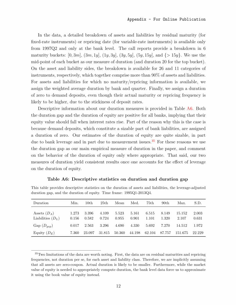
Appendix – For Online Publication
In the data, a detailed breakdown of assets and liabilities by residual maturity (forfixed-rate instruments) or repricing date (for variable-rate instruments) is available onlyfrom 1997Q2 and only at the bank level. The call reports provide a breakdown in 6maturity buckets: [0, 3m], (3m, 1y], (1y, 3y], (3y, 5y], (5y, 15y], and {> 15y}. We use themid-point of each bucket as our measure of duration (and duration 20 for the top bucket).On the asset and liability sides, the breakdown is available for 26 and 11 categories ofinstruments, respectively, which together comprise more than 90% of assets and liabilities.For assets and liabilities for which no maturity/repricing information is available, weassign the weighted average duration by bank and quarter. Finally, we assign a durationof zero to demand deposits, even though their actual maturity or repricing frequency islikely to be higher, due to the stickiness of deposit rates.
Descriptive information about our duration measures is provided in Table A6. Boththe duration gap and the duration of equity are positive for all banks, implying that theirequity value should fall when interest rates rise. Part of the reason why this is the case isbecause demand deposits, which constitute a sizable part of bank liabilities, are assigneda duration of zero. Our estimates of the duration of equity are quite sizable, in partdue to bank leverage and in part due to measurement issues.35 For these reasons we usethe duration gap as our main empirical measure of duration in the paper, and commenton the behavior of the duration of equity only where appropriate. That said, our twomeasures of duration yield consistent results once one accounts for the effect of leverageon the duration of equity.
Table A6: Descriptive statistics on duration and duration gap
This table provides descriptive statistics on the duration of assets and liabilities, the leverage-adjustedduration gap, and the duration of equity. Time frame: 1995Q1-2013Q4.
Duration Min. 10th 25th Mean Med. 75th 90th Max. S.D.
Assets (DA) 1.273 3.396 4.109 5.523 5.161 6.515 8.149 15.152 2.003Liabilities (DL) 0.156 0.582 0.724 0.955 0.901 1.101 1.320 2.107 0.631
Gap (Dgap) 0.017 2.563 3.296 4.690 4.330 5.692 7.270 14.512 1.972
Equity (DE) 7.360 23.097 31.815 50.360 44.198 62.104 87.757 151.675 22.229
35Two limitations of the data are worth noting. First, the data are on residual maturities and repricingfrequencies, not duration per se, for each asset and liability class. Therefore, we are implicitly assumingthat all assets are zero-coupon. Actual duration is likely to be smaller. Furthermore, while the marketvalue of equity is needed to appropriately compute duration, the bank level data force us to approximateit using the book value of equity instead.
12


