Risk-Averse Capacity Planning for Renewable EnergyProduction

Bo Sun� Pavlo Krokhmal� Yong Chen�

Abstract

This paper considers the problem of capacity planning and operation of energy grids where the powerdemands are served from renewable energy sources, such as wind farms, and the transmission networkis represented by the High-Voltage Direct Current (HVDC) lines. The principal question considered inthis work is whether a risk-averse design of the grid, including the selection of wind farm locations andassignment of power delivery from wind farms to customers, would allow for effective hedging of the risksassociated with uncertainties in power demand and production of energy from renewable sources.

To this end, the problem is formulated in the general context of supply chain/facility location, with boththe supply and the demand being stochastic variates. Several stochastic optimization models are presentedand analyzed, including the traditional risk-neutral, or expectation-based model and risk-averse modelsbased on linear and nonlinear coherent measures of risk. Exact solutions algorithms that employ Bendersdecomposition and polyhedral approximations of nonlinear constraints have been proposed for the obtainedlinear and nonlinear mixed-integer programming problems. The conducted numerical experiments illustratethe properties of the constructed models, as well as the efficiency of the developed algorithms.

Keywords: Capacity planning, facility location, stochastic supply, coherent measures of risk, Bendersdecomposition, mixed integer p-order cone programming

1 Introduction

The need for effective energy harvesting from renewable resources becomes increasingly important, espe-cially in view of the inevitable depletion of the fossil fuel energy sources. Among renewable energy sources,wind energy represents one of the most attractive alternatives due to a multitude of factors, including theavailability of a relatively mature technology for energy harvesting, a broad range of geographical locationsand climates that are suitable for industrial-scale wind power generation, and so on. As a result, the windenergy industry has recently experienced significant worldwide growth. In 2014, the global wind power in-stalled capacity has reached an estimated 336,327 megawatts (MW), which can satisfy around 4% of theworld’s electricity demand [67].

In the United States, the wind energy industry has been one of the fastest growing sectors of economy in thelast several years. In 2013, the electricity produced from wind power accounted for 4.13% of all generatedelectrical energy in the U.S., and became the fifth largest electricity source according to the data from theU.S. Department of Energy’s Energy Information Administration (EIA). A technical report from NationalRenewable Energy Laboratory (NREL) [33] indicates that the United States have the total estimated onshorewind energy potential for 10,955 GW, which could produce 32,784 TWh annually, amounting to almosteight times of total U.S. electricity consumption in 2011. In addition, the offshore wind energy potential isestimated to be 4,150 GW [51]. The U.S. Department of Energy projected that by 2030 wind power couldsatisfy 20% of total electricity demand in the U.S.

�Department of Mechanical and Industrial Engineering, University of Iowa, Iowa City, IA 52242, USA�Department of Systems and Industrial Engineering, University of Arizona, Tucson, AZ 85721, USA, e-mail:

krokhmal@email.arizona.edu (corresponding author)

1

On the other hand, the advantages of wind as a renewable and commonly available source of energy comeat a cost of uncertainty in the amount of wind power that can be produced during any given time period. Inthis respect, power production using renewable energy sources differs drastically from the traditional powerproduction using fossil fuel sources, whose reserves can be accurately estimated and utilized in a controlledmanner. As a result, the design and operation of the existing power infrastructure, which implicitly relieson the presumption that power production is completely controllable, may not be ideally suited for the casewhen a significant portion of generated and consumed power comes from renewable energy sources, such aswind.

In this work, we consider the problem of strategic capacity planning for power grids that are based exclusivelyon wind energy sources, and the primary issue that we aim to elucidate is the problem of effective control ofrisks of power shortages due to the uncertainties in wind power production and power demands. Specifically,the question of interest is whether a risk-averse approach to power capacity planning can be effective forhedging the risks of power shortages due to stochastic variations in power generation and demand.

To this end, we cast the problem of capacity planning for renewable energy power production as a supplychain problem where both the supply and demand for a specific product (i.e., electric power) are highlystochastic. In particular, we adopt the setting of a stochastic wind farm location model, and employ a class of(generally nonlinear) statistical functionals known as coherent measures of risk to quantify and minimize therisks of unsatisfied power demand via optimal selection of sites for wind energy harvesting and matching ofenergy producers and customers.

We consider our analysis to be at the strategic level as it pertains to planning and operation at the relativelylong-term monthly scale with respect to the power generation and demand. The assumption that all powerdemand within the grid is served by renewable wind energy sources implies that these sources must representlarge-scale, massive wind farms. In addition, we assume that the generated electricity is transmitted to de-mand nodes through high-voltage direct current (HVDC) lines. HVDC transmission lines are used to transmitbulk of electrical energy over long distances by means of direct current (DC), in contrast to the more commonalternating current (AC) used in most of today’s electrical transmission infrastructure. Since there is no needfor reactive compensation along the transmission line, the HVDC lines typically lose less power than equiv-alent AC transmission lines. This, in addition to lower transmission costs, makes HVDC more economicalthan AC transmission for large amounts of power transmitted over long distances. Moreover, HVDC trans-mission can improve system’s stability since it allows the operator to quickly change the direction of powerflow, as well as allows for the power transportation between power systems with different frequencies. Thesecharacteristics of HVDC transmission make it an appealing choice for renewable energy grids with wind orsolar energy sources, as it could aid in mitigating the effects of intermittency and fluctuation and smooththe power outputs, as well as improve the economic viability of renewable energy due to lower transmissioncosts.

In conclusion of our introductory remarks, we would like to note that the problem setting adopted in this workis more “futuristic” than “realistic”, in the sense that industrial-scale power grids where the power is generatedentirely from renewable energy sources are unlikely to appear in the foreseeable future. At the same time,we believe that tapping into the idea of building and utilizing a power infrastructure that employs exclusivelyrenewable energy is of scientific and engineering interest, and the present work represents a contribution inthis direction. In addition, the obtained results are expected to be of more immediate and practical value inthe context of supply chains with stochastic supply and demand.

Finally, we would like to mention that the general model developed in this work is potentially applicable tocapacity planning of power production from other types of renewable energy where weather patterns are ofsignificant influence, such as solar energy and ocean wave energy.

The remainder of this paper is organized as follows. Section 2 contains a review of relevant literature. InSection 3, we formulate three stochastic wind farm location models with different degrees of risk aversion.Branch-and-bound solution algorithms for the resulting mixed-integer linear and nonlinear programmingproblems, which employ Benders decomposition method and outer polyhedral approximations of nonlinearconstraints, are presented in Section 4. Section 5 discusses dataset generation, computational results, and the

2

corresponding solution analysis.

2 Literature Review

The problem of configuration of power generating systems with renewable energy and storage has been ex-tensively studied. In [53], a genetic algorithm has been proposed to determine the optimal configuration ofpower system in isolated island with installed renewable energy power plants. Katsigiannis and Georgilakis[27] performed tabu search to solve a combinatorial problem which aimed to optimize sizing of small isolatedhybrid power systems. Similarly, Ekren and Ekren [23] applied simulated annealing method for achieving theoptimal size of a PV/wind integrated hybrid energy system with battery storage. In addition to these heuristicsmethods, stochastic programming models have also been employed to design the energy system. Abbey andJoos [1] put forward a stochastic mixed integer programming model to optimize sizing of storage system foran existing isolated wind-diesel power system. In [32], a multi-stage stochastic mixed integer programmingmodel has been presented for a comprehensive hybrid power system design by including renewable energygeneration. More particularly, Burke and O’Malley [13] considered the problem which sought to find theoptimal locations to incorporate wind capacity on an existing transmission system network. A portfolio ap-proach to optimal wind power deployment in Europe has been studied by Roques et al. [48], who endeavoredto smooth out the fluctuations through geographic diversification of wind farms.

This paper considers the strategic-level capacity planning of renewable energy power grids in the contextof a supply chain view of the power infrastructure, and particularly, with respect to the degree to which thepower production in the renewable energy grid is capable of meeting the consumers’ power demands. Fromthe supply chain point of view, facility location decisions constitute the strategic level of planning [37, 58]and as such represent a crucial factor in reliability and resilience of supply chain operations [35], see also[25, 49, 55].

The key feature of our model is the presence of uncertainties in both demand and supply of electric power.While the literature on strategic facility location and supply chain planning under uncertainties is extensive(see, for example, comprehensive reviews [42, 59] and references therein), majority of the works considerdemand-side uncertainty, stochastic costs, travel times, etc.

Here we briefly mention some of the developments most relevant to the present approach. Sheppard [57]presented one of the first scenario-based models of facility location under uncertainties; a stochastic 2-medianfacility location problem on a probabilistic tree network was first considered in Mirchandani and Oudjit[38]. Weaver and Church [66] and Mirchandani et al. [39] further discussed stochastic versions of p-medianlocation problem and developed solution methods based on Lagrangian relaxation. Louveaux [34] proposedthe stochastic versions of the capacitated p-median problem and capacitated fixed-charge location problemwith uncertain demands, prices and costs. Berman and Drezner [10] considered a variation of stochasticp-median problem, where additional facilities with knownn probabilities would be located in the future. The˛-reliable minimax regret model, which minimized the ˛-quantile of all regrets was proposed by Daskin et al.[20] . A facility location model which solved for the minimum expected cost while kept relative regret undereach scenario limited (p-robust), was formulated by Snyder and Daskin [62]. Chen et al. [16] introduced amodel called ˛-reliable mean-excess regret that instead minimized the expected regret of the “tail” of costdistribution. Robust optimization of a multi-period facility location problem with stochastic demand wasdiscussed in Baron et al. [6].

Literature on supply chain models with stochastic supply is more limited. Among the forms of supply un-certainty that are typically considered, such as supply disruptions, yield uncertainty, capacity uncertainty,and lead time uncertainty (see Snyder et al. [60] for a thorough discussion of these and other aspects), thesupply disruptions represent, perhaps, the most commonly discussed factor in supply uncertainties. For exam-ple, Drezner [22] considered the supply disruptions for facility location problem by presenting two models,unreliable p-median and (p, q)-center problem where at most q facilities might fail. Reliable versions ofp-median and uncapacitated fixed-charge location problem were proposed by Snyder and Daskin [61], which

3

took the expected cost after failures of facilities into consideration. Berman et al. [11] and Shen et al. [56]studied problems similar to [61], but considered heterogeneous disruption probabilities. Also taking accountof site-dependent disruption probabilities, Cui et al. [19] studied the reliable uncapacitated fixed-charge loca-tion problem through a mixed-integer model and a continuum approximation, respectively. A mixed-integermodel for network design with supply disruption, which minimized the nominal cost while bounding the costwith p-robustness, was proposed by Peng et al. [43].

With regard to supply chain models with uncertain demand and supply, Santoso et al. [49] proposed a stochas-tic programming model for the supply chain network design problem, where the objective function was tominimize the investment and operation costs. Processing/transportation costs, demands, supplies, and capac-ities were assumed to be stochastic and jointly distributed. Azaron et al. [4] considered a similar model forsupply chain design but with multiple objectives, which additionally included the minimization of the vari-ance of the total cost and minimization of the financial risk. A two-stage stochastic program for the supplychain design was formulated by Schutz et al. [50], which involved strategic location decisions in the firststage and operational decisions in the second stage, and where both short-term and long-term uncertaintieswere considered. Baghalian et al. [5] developed a stochastic model to design a multi-product supply chainnetwork, where supply disruption and demand uncertainty were taken into account simultaneously.

In view of the above, the contributions of the present work can be delineated as follows. In contrast to afore-mentioned papers [4, 5, 49, 50], where a penalty multiplier approach was used to quantify the unsatisfieddemand, we employ linear and nonlinear coherent measures of risk to deal with power shortages. In addition,our wind farm location model involves discrete capacity variables at each location, which represent the num-ber of wind turbines to install. From the viewpoint of power grids literature, the present work provides oneof the relatively few accounts of risk-averse design and operation of power grids, and especially renewableenergy grids. Finally, from the computational point of view, this paper furnishes an efficient exact solutionmethod for solving the obtained nonlinear p-order cone mixed integer programming models, which combinesthe branch-and-bound method based on polyhedral approximations for conic mixed integer problems due toVielma et al. [63] and Vinel and Krokhmal [64] with Benders decomposition method.

3 Stochastic Wind Farm Location Models

In this section, we introduce several stochastic optimization models that address the problem of strategiclocation of wind farms so as to satisfy the power demand at a given set of demand sites at a minimum cost.In all models, it is assumed that both the power demand and power generation are uncertain, or stochastic.To model these sources of uncertainty, we adopt the scenario-based approach that is traditional in stochasticprogramming literature, i.e., we assume that the set of random events � in the probability space .�;F ;P/ isdiscrete,� D f!1; : : : ; !Kg, where each elementary random event, or scenario !k has a non-zero probabilityPf!kg D �k > 0, such that

Pk �k D 1.

Below we present a generic stochastic model (GS) that allows for satisfying the expected demand in each bus(demand node) of the power grid. To this end, we introduce the following notations:

i W index of demand nodes;j W index of candidate sites of wind farms;k W index of scenarios;h W number of wind farms to locate; W cost of power shortages;� W annual amortized cost per mile of HVDC transmission line built;~ W power loss per mile of HVDC line;Mj W an upper bound on the number of wind turbines that can be installed at a given candidate site j ;fj W annual amortized fixed cost of wind farm site j ;

4

cj W annual amortized cost of per turbine purchased and installed at site j ;�k W probability of scenario kdij W distance from node i to candidate site j ;Qjk W power output of a wind turbine in candidate site j under scenario k;Dik W power demand at node i under scenario k;

Di W expected power demand at node i .

Also, we define the following decision variables:

xj W binary variable indicating whether wind farm site j is selected;yij W binary variable indicating whether demand node i is connected to wind farm site j ;�ij W number of turbines at wind farm site j serving demand node i ;qijk W power generated at wind farm site j serving demand node i under scenario k.

3.1 A Generic Stochastic Model for Wind Farm Location

Using the above notations, a generic stochastic model for strategic wind farm location under uncertainties(GS) can be presented in the form of a mixed-integer linear programming problem:

minXj

fjxj CXi

Xj

cj �ij CXi

Xj

�dijyij (1a)

s. t.Xj

xj D h; (1b)

yij � xj ; 8i; j; (1c)�ij �Mjyij ; 8i; j; (1d)qijk � Qjk�ij ; 8i; j; k; (1e)Xk

�kXj

.1 � ~dij /qijk � Di ; 8i; (1f)

xj ; yij 2 f0; 1g; �ij 2 ZC; qijk 2 RC; 8i; j; k: (1g)

Objective function (1a) represents the cumulative annual cost to be minimized. Constraint (1b) stipulates,without loss of generality, that exactly h wind farms are to be located; in the cases when the number ofwind farms is allowed to vary, equality in (1b) can be relaxed, or the constraint (1b) itself can be omitted.Constraint (1c) states that a demand node i cannot be assigned to a wind farm j unless a wind farm is locatedat site j . Constraint (1d) limits the number of wind turbines at site j that can be assigned for serving busi . Constraint (1e) ensures that power supplied by site j to bus i under scenario k does not exceed the totalcapacity of all wind turbines assigned at site j to serving bus i . Constraint (1f) ensures that the expectedpower supplied to bus i from all sites does at least meet the expected demand at bus i . Lastly, constraint (1g)determines the values that decision variables take, where ZC and RC denote the sets of non-negative integerand real numbers, respectively. In what follows, the feasible set defined by constraints (1b)–(1g) is denotedby P .

Remark 1 Note that the wind farm location model (1) does not include the power flow constraints [15, 21],which define the physically feasible distribution of power in an electric grid, and relate the real and thereactive power, the voltage magnitudes and phases (angles) at each bus in the grid. In accordance to thediscussion of the goals of this work in Introduction, the stochastic programming formulation (1) models theoperation of a renewable energy grid at a long-term scale, where each scenario reflects averaged figures ofpower production and demand over a relatively long time frame (one month in our case study, see Section 5).

5

In contrast, Kirchhoff’s Circuit Laws that underlie the power flow constraints are formulated with respect toexact temporal values of currents and voltages in electrical circuits. The purpose of the generic stochasticmodel (1), as well as the risk-averse models stochastic that are described below and are derived from (1), isto elucidate the capacity-related aspects of the operation of power infrastructure where stochastically variablepower production must be used to satisfy stochastic power demand. At the same time, since it is assumedthat power is distributed in our grid via HVDC transmission lines, the DC power flow constraints reduce tolinear constraints, and as such can be easily incorporated into the formulated models for a study of powerdistribution in the grid at shorter time scales. The corresponding solutions algorithms, presented in Section 4,will still be applicable.

3.2 Risk-Averse Models for Strategic Wind Farm Location

It is easy to see that the generic stochastic optimization model (1) is prone to substantial power shortages,which may occur in particular scenarios when the power load at bus i and/or the amount of power supplied tothis bus deviate from the corresponding average figures. This is a consequence of the well-known propertiesof stochastic optimization models where constraints are satisfied “on average” [29]. In order to avoid powershortages, one may require that power load at each bus i be satisfied at every scenario !k 2 �, which can bewritten as

maxk

�Dik �

Xj

.1 � ~dij /qijk

�� 0; 8i: (2)

This method, also known as “robust optimization” approach [28], has been acknowledged in the literature assuch that can often lead to overly conservative and exceedingly costly solutions [29]. In addition, enforcingthe last constraint does not guarantee shortage-free power distribution in practice, since the scenario datarepresents only a finite sample from the generally unknown distributions of power demand and wind powerproduction.

In this work, we pursue a risk-averse stochastic optimization approach which is supposed to avoid the po-tentially large power shortages associated with the expected-value constraint (1f) as well as the high costsassociated with the “robust” constraints (2) by explicitly accounting for the risks of power shortages.

To quantify the risk of power shortages that may have large magnitudes but very low probabilities of occur-ring, we employ a class of statistical functional known as coherent measures of risk [3], and, more specifically,the well-known Conditional Value-at-Risk (CVaR) measure [47] and its nonlinear generalizations, HigherMoment Coherent Risk (HMCR) measures [30].

Technically, a risk measure is a function � W X 7! R, where X is an appropriately defined linear space ofF-measurable functions X W � 7! R. Further definition of risk measures �.X/ typically requires specifyingwhether the larger or smaller realizations of random element X are considered to be “risky”. Here we adoptthe setup common in engineering literature, where the random variable X D X.x; !/ is assumed to representthe cost or loss associated with the decision x, and thus smaller realizations ofX are preferred (the alternativeassumption, that X represents a payoff or a reward, is prevalent in economics and finance domains).

Then, �.X/ as defined above is said to be a coherent measure of risk [3, 29] if it satisfies the additionalproperties of monotonicity, �.X1/ � �.X2/ for all X1 � X2; sub-additivity, �.X1 CX2/ � �.X1/C �.X2/;positive homogeneity, �.�X/ D ��.X/ for a constant � > 0; and translation invariance, �.XCc/ D �.X/Cc for any c 2 R. The monotonicity property asserts that smaller losses bear less risk. The sub-additivityproperty in combination with positive homogeneity provides for convexity of coherent risk measures, whichentails that coherent measures of risk allow for risk reduction via diversification, and, importantly, admitefficient optimization of risk via the methods of convex programming. The translation invariance propertyallows for efficient risk hedging, see [3] for a detailed discussion.

From this definition, it is easy to see that the risk measure defined as �.X/ D EX is coherent. Hence, if onedefines the stochastic cost/loss functionX as the energy shortage at site i ,Xi .!k/ D Dik�

Pj .1�~dij /qijk ,

6

then constraints (1f) stipulating that power demand at each bus i must be satisfied on average, can equivalentlybe interpreted as the requirement of non-negative risk of power shortages at each bus i ,

�.Xi / � 0; 8i; (3)

where �.X/ D EX . Similarly, another trivial instance of coherent measures of risk is represented by the“maximum loss” measure, �.X/ D maxX , which associates the risk of a stochastic loss or cost X with itslargest possible realization (it is assumed here that the distribution ofX has a bounded support, in the generalcase the maximization operator in the definition of this risk measure must be replaced with the essentialsupremum, �.X/ D ess supX , see, e.g., [29] for details). Then, the conservative-but-costly approach ofensuring that power demands are satisfied at every scenario, embodied by constraints (2), reduces to the riskconstraints of the same form (3) where � is selected as the maximum loss measure.

In order to find, as we have proposed above, an effective – both methodologically and computationally –compromise between the “loose”, risk-neutral expectation-based constraints (1f) and the most conservativerisk-averse constraints (2), we will employ the well-known Conditional Value-at-Risk (CVaR) measure [47].For a given confidence level ˛ 2 .0; 1/, Conditional Value-at-Risk CVaR˛.X/ can be interpreted as theexpected cost or loss that can occur with probability 1�˛ over the prescribed time horizon, or as the averageof the .1 � ˛/ � 100% of the largest (worst) realizations of the stochastic loss factor X . This interpretationis reflected in the fact that for a continuously distributed X , CVaR˛.X/ can be represented in the form ofconditional expectation

CVaR˛.X/ D EŒX j X � F �1X .˛/�; (4)

where FX .t/ denotes the cumulative distribution function of X , and F �1X .˛/ is the ˛-quantile of X , or sucha deterministic value that can be exceeded by X with probability 1 � ˛. In financial and risk managementliterature the ˛-quantile is also known as the Value-at-Risk at the confidence level ˛, VaR˛.X/.

In the case of general distributions of X , definition (4) does not apply, in the sense that the correspondingconditional expectation is not guaranteed to have coherence properties [47]. It has been shown in [47] thatin the general case CVaR˛.X/ can be represented as a convex combination of F �1˛ .X/ and the conditionalexpectation of losses strictly exceeding F �1˛ .X/, with weight coefficients dependent on both X and ˛. Amore computationally attractive definition of CVaR for general loss distributions presents it as the optimalvalue of the following unconstrained convex optimization problem [46, 47]:

CVaR˛.X/ D min�2R

�C .1 � ˛/�1E.X � �/C; (5)

where X˙ D maxf0;˙Xg. Besides being a coherent measure of risk, CVaR˛.X/ possesses a number ofother properties, such as, for example, continuity with respect to the confidence level ˛. In the context of ourdiscussion, another notable property of the CVaR measure is that, as a function of the parameter ˛, it includesboth �.X/ D EX and �.X/ D ess supX as special cases:

lim˛!0

CVaR˛.X/ D EX; lim˛!1

CVaR˛.X/ D ess supX: (6)

Hence, to achieve a balance between the “risk-neutral” approach of ensuring that power shortages do not oc-cur on average, and the “absolute risk-averse” approach requiring that power shortages never occur, one mayquantify the risk of power shortages using CVaR measure with an appropriately selected value of confidencelevel ˛ 2 .0; 1/, whereby the shortage risk would be represented by the average of .1 � ˛/ � 100% largestshortages.

To incorporate the quantification of risks of power shortages in the wind farm location model (1) via theConditional-Value-at-Risk measure, we define the cost/loss function X as the cumulative power shortageover all buses,

X.!k/ DXi

�Dik �

Xj

.1 � ~dij /qijk

�C

; 8k: (7)

7

In order to have an additional degree of flexibility in our model, we include CVaR˛.X/ in the objective ofproblem (1) with an appropriate weight coefficient > 0, which represents the cost (in millions of dollars)of 1MW of power short:

minXj

fjxj CXi

Xj

cj �ij CXi

Xj

�dijyij C CVaR˛.X/

s. t. xj ; yij ; �ij ; qijk 2 P;

where X is defined by (7). Note that the cost of shortages in the objective function is non-negative due tothe fact that X.!k/ � 0 in (7). By further defining auxiliary variables Uk and �, the risk-averse CVaR-basedstochastic model (CVaRS) can be formulated as follows:

minXj

fjxj CXi

Xj

cj �ij CXi

Xj

�dijyij C

��C

1

1 � ˛

Xk

�kUk

�(8a)

s. t. Uk �Xi

�Dik �

Xj

.1 � ~dij /qijk

�C

� �; 8k; (8b)

Uk 2 RC; 8k; (8c)xj ; yij ; �ij ; qijk 2 P : (8d)

By means of the Conditional Value-at-Risk measure, the risk-averse formulation (8) accounts for the risk ofpower shortages as the first moment of the .1 � ˛/-tail of the shortages distribution. At the same time, the“risk” as a proxy for “large losses that have a low probability of occurring” is commonly associated in therisk management literature with “heavy tails” of distributions, and the distributions of power shortages arewell known to be heavy tailed (see, e.g., [17, 26, 36]). Therefore, it is of interest to take into account highermoments of shortage distribution in assessing the risk of power shortages. This can be accomplished withthe help of the family of Higher-Moment Coherent Risk (HMCR) measures [30]. Assuming that the spaceX admits a sufficient degree of integrability, i.e., X D Lp.�;F ;P/ for a given p � 1, the HMCR measuresare defined as

HMCRp;˛.X/ D min�2R

�C .1 � ˛/�1k.X � �/Ckp; p � 1; ˛ 2 .0; 1/; (9)

where kXkp D .EjX jp/1=p . Obviously, the HMCR family contains CVaR as a special case of p D 1.

Similarly to CVaR-based formulation (8), minimization of the total cost that includes the shortage risk cost asexpressed by a higher tail moment of shortage distribution is given by the following HMCR-based stochasticoptimization (HMCRS) model:

minXj

fjxj CXi

Xj

cj �ij CXi

Xj

�dijyij C ��C .1 � ˛/�1U0

�(10a)

s. t. q�1=p

kUk �

Xi

�Dik �

Xj

.1 � ~dij /qijk

�C

� �; 8k; (10b)

U0 ��Up1 C : : :C U

pK

�1=p; (10c)

t � 0I Uk � 0; 8k; (10d)xj ; yij ; �ij ; qijk 2 P : (10e)

The nonlinear inequality (10c) represents a p-order cone constraint, whence formulation (10) representsa mixed-integer p-order cone programming (MIpOCP) problem. The next section discusses the solutionmethods for the proposed risk-averse stochastic wind farm location models CVaRS (8) and HMCRS (10), aswell as their special case, the risk-neutral GS model (1).

8

4 Benders Decomposition Based Branch-and-Bound Algorithms

The introduced above stochastic wind farm location models GS (1), CVaRS (8) and their generalization HM-CRS (10) are formulated as mixed-integer linear (in the case of HMCRS, nonlinear) programming problems,and as such admit a variety of solution techniques, see, e.g., [12, 54], and references therein. In this work,we employ the Benders decomposition method [12, 44, 45, 54] as the basic approach to solving both linearand nonlinear mixed-integer problems (1), (8), and (10). Benders decomposition is one of the most popularalgorithmic frameworks in stochastic optimization, and it has been widely applied to many energy-relatedstochastic programming problems (see a recent review [45] and references therein). In what follows we showthat this technique works well on the linear models (1) and (8); however, our ultimate goal in this section isto construct an efficient solution method for the more general nonlinear MIpOCP formulation (10). A dis-cussion of solution approaches to mixed-integer programming problems with cone constraints can be foundin, for example, [65]. In section 4.3, we propose an efficient algorithm for (10) that integrates the Bendersdecomposition method into a branch-and-bound scheme for general MIpOCP problems that is based on poly-hedral approximation of cone constraints [63, 64], thereby exploiting the structural properties of problem (10)induced by the location variables and constraints and the cone constraints. In order to make the expositionstreamlined and self-contained, we first discuss the general Benders decomposition method for the linearproblems (1) and (8).

4.1 General Formulations

The discussed formulations of GS andf CVaRS models can be generally written as mixed-integer linearprogramming programming problems of the form

Z D min a>zC b>u (MILP)s. t. AzC Bu � c;

z 2 Z � ZmC; u 2 R`C;

where z and u represent an m-dimensional vector of integer variables and an `-dimensional vector of contin-uous variables, and Z is a bounded subset of ZmC. Assume that problem MILP is bounded and feasible. Then,it can be equivalently represented as

Z D min a>zC t .z/ (11a)s. t. z 2 Z; (11b)

where for any given z 2 Z , function t .z/ is defined to be the optimal objective value of the linear program-ming problem

t .z/ D min b>u (12a)s. t. Bu � c � Az; (12b)

u � 0: (12c)

Note that since set Z � ZmC is bounded, the unboundedness of the original problem MILP is associated withthat of problem (12). By introducing dual variables �, we can calculate t .z/ through solving its dual problem,under the assumption of boundedness of problem (12). The dual of problem (12) is

t .z/ D max .c � Az/>� (SMILP)

s. t. B>� � b;� � 0:

If the feasible region of problem SMILP is empty, then the primal subproblem (12) is either unbounded orinfeasible, which implies the unboundedness or infeasibility of the original problem MILP. Otherwise, we can

9

enumerate all extreme points .�1p ; : : : ; �Ip /, and extreme rays .�1r ; : : : ; �

Jr / of the feasible region of SMILP,

where I and J denote the numbers of extreme points and extreme rays. Therefore, the dual subproblemSMILP can be rewritten as

t .z/ D min t (13a)

s. t. .c � Az/>�jr � 0; 8j D 1; : : : ; J; (13b)

.c � Az/>�ip � t; 8i D 1; : : : ; I; (13c)

t 2 R: (13d)

By replacing t .z/ in problem (11) with that given by formulation (13), we obtain a reformulation of theoriginal problem MILP:

min a>zC t (RMILP)

s. t. .c � Az/>�jr � 0; 8j D 1; : : : ; J;

.c � Az/>�ip � t; 8i D 1; : : : ; I;

z 2 Z; t 2 R:

We denote problem RMILP but only with a subset of constraints (13b) and (13c) as problem MMILP, repre-senting the master problem of mixed-integer linear programming problem MILP.

The standard Benders decomposition scheme is then invoked, which consists in solving the “relaxed” problemMMILP (as usual, the procedure is initialized by solving MMILP without any constraints (13b) and (13c) andthe variable t in its objective disregarded). If it is unbounded, let ��r be the column vector in which all thecorresponding simplex multipliers are negative, after simplex terminates. Therefore, ��r is an extreme ray ofthe feasible region of SMILP, whence a feasibility cut

.c � Az/>��r � 0 (14a)

is added to MMILP and the problem is thus resolved until an optimal solution .z�; t�/ of MMILP is obtained.Subsequently, the dual subproblem SMILP is solved for the given z�, and let ��p be the corresponding optimalsolution, or an extreme point of its feasible region. If t .z�/ D .c � Az�/>��p > t�, then problem MMILP isaugmented with the optimality cut

.c � Az/>��p � t (14b)

and resolved.

The decomposition procedure stops when the condition t .z�/ D t� is satisfied. During each iteration, afeasibility or optimality cut is added, and an optimal solution of RMILP is obtained in a finite number ofiterations due to finiteness of I and J [9]. The following two propositions follow readily from the abovediscussion.

Proposition 1 If Qz 2 Z and there is an optimal solution to the dual subproblem SMILP with objective valueQt D maxf.c � AQz/>� W B>� � b; � � 0g, then a> QzC Qt is an upper bound on the optimal solution value ofproblem RMILP.

Proposition 2 Assume that .z�; t�/ is an optimal solution of the master problem MMILP. If the optimalobjective value of the corresponding problem SMILP is equal to t�, i.e., t� D maxf.c � Az�/>� W B>� �

b; � � 0g, then .z�; t�/ is an optimal solution to the equivalent reformulation of the original problem RMILP.

4.2 Benders Decomposition Based Algorithm for GS and CVaRS Models

In the following, we denote problems MMILP and RMILP with relaxed integrality constraints (namely, z 2Z � ZmC replaced by z 2 conv.Z/ � RmC) as problem MLP and problem RLP, respectively. Furthermore,

10

we define a node n in the branch-and-bound tree by a triple .zn; Nzn; Zn/ 2 Z2mC � .R [ fC1g/, where.zn; Nzn/ are the bounds on z at node n and Zn is a lower bound on ZMLP.zn;Nzn/. The problem MLP.zn; Nzn/is defined as the problem MLP with added constraints zn � z � Nzn, and ZMLP.zn;Nzn/ is the correspondingoptimal objective value. Similarly, for any Ozn 2 ZmC we denote by SMILP.Ozn/ by replacing the variable z withthe value Ozn in problem SMILP, and by ZSMILP.Ozn/ the corresponding optimal objective value. In addition,we introduce Z and N to denote the global upper bound on ZRMILP and the set of active branch-and-boundnodes, respectively. The algorithm is described as follows (see Algorithm 1 for details).

Step 1 Initialize the set of active branch-and-bound nodes N with root node defined as .z0; Nz0; Z0/, andglobal upper bound Z with positive infinity.

Step 2 Select and remove a node from the set N .

Step 3 Solve problem MLP.zn; Nzn/.

Step 4 If the solution of problem MLP.zn; Nzn/ is feasible and its optimal objective value is less than thecurrent global upper bound Z, go to Step 5; otherwise, fathom this node and go to Step 2.

Step 5 Denote the optimal solution to problem MLP.zn; Nzn/ by .Ozn; Otn/. If the values of Ozn are all integers,go to Step 6; otherwise, branch on this node and go to Step 2.

Step 6 Solve the problem SMILP.Ozn/. If its optimal objective value equal to Otn obtained in Step 5, thenupdate the global upper bound Z and incumbent solution, and fathom this node; otherwise, go to Step7.

Step 7 Check the solution status of problem SMILP.Ozn/, if it is unbounded, then add a feasibility cut toproblem MLP.zn; Nzn/, go to Step 3; otherwise, check whether ZSMILP.Ozn/ > Ot

n, if it is true, then addan optimality cut to problem MLP.zn; Nzn/, go to Step 3.

Proposition 3 The Benders decomposition based branch-and-bound algorithm for GS and CVaRS modelsterminates with the upper bound Z equal to the optimal objective value of original problem MILP.

Proof: The proof is omitted and is analogous to that of the more general Proposition 4 presented in Sec-tion 4.3.1. �

Appendices A.1 and A.2, respectively, present the explicit expressions for the feasibility and optimality cutsthat arise in the process of solving the GS and CVaRS models using the described above algorithm.

4.3 HMCRS Model as a Mixed-Integer p-Order Cone Programming Problem

Due to the presence of the p-order cone constraint in formulation (10),

U0 � .Up1 C : : :C U

pK /

1=p; (15)

the HMCRS model represents a mixed-integer p-order cone programming problem (MIpOCP). Below wepropose an algorithm for the MIpOCP HMCRS problem that combines the Benders decomposition witha general branch-and-bound algorithm for solving MIpOCP problems that was presented in Vinel andKrokhmal [64]. The idea of the latter method involves solving a polyhedral approximation of the integerrelaxation of MIpOCP problem at each node of the BnB tree, and is based on the work of Vielma et al. [63]for mixed integer second order cone programming problems (MISOCP).

Let pOCP denote the integer relaxation of the original MIpOCP problem. Then, a polyhedral approximationof the pOCP relaxation is obtained by replacing nonlinear p-order cone constraints with their polyhedral

11

Algorithm 1 A Benders decomposition based branch-and-bound algorithm for GS and CVaRS models

1: Set global upper bound Z WD C1; set Z0 WD �12: Set ´0

rWD �1, N0r WD C1 for all r 2 f1; : : : ; mg; initialize node list N WD f.z0; Nz0; Z0/g

3: while N ¤ ; do4: Select and remove a node .zn; Nzn; Zn/ from N5: Solve MLP.zn; Nzn/6: if MLP.zn; Nzn/ is feasible and ZMLP.zn;Nzn/ < Z then7: Let .Ozn; Otn/ be the optimal solution to MLP.zn; Nzn/8: if Ozn 2 ZmC then9: Solve SMILP.Ozn/

10: if ZSMILP.Ozn/ D Otn then

11: Z WD ZMLP.zn;Nzn/; update incumbent solution12: else13: if SMILP.Ozn/ is unbounded then14: Add feasibility cut (14a) to MLP.zn; Nzn/; go to 515: if ZSMILP.Ozn/ > Ot

n then16: Add optimality cut (14b) to MLP.zn; Nzn/; go to 517: else18: Select r0 in fr 2 f1; : : : ; mg W Onr … ZCg

19: Let ´rWD ´n

r, N r WD Nnr for all r 2 f1; : : : ; mgnfr0g

20: Let N r0 WD b Onr0c, ´

r0WD b Onr0

c C 1

21: N WD N [˚�

zn; Nz; ZMLP.zn;Nzn/�;�z; Nzn; ZMLP.zn;Nzn/

�22: Remove every node .zn; Nzn; Zn/ 2 N such that Zn � Z23: end while

12

approximations. It is crucial, however, that such a polyhedral approximation be “compact” with respect tothe number of facets, since a straightforward approximation of a p-cone in RKC1 by tangent hyperplanesrequires O.2K/ facets. To this end, a lifted representation of a multidimensional p-cone is used [8, 64],which expresses a p-cone in RKC1C as an intersection of K � 1 three-dimensional p-cones:

U2K�1 D U0; UKCk � .Up

2k�1C U

p

2k/1=p; k D 1; : : : ; K � 1: (16)

Then, it is easy to see that if each of the three-dimensional p-cones is replaced by its polyhedral approxima-tion with O.L/ facets, the resulting polyhedral approximation of multidimensional p-cone (15) will containno more than O.KL/ facets. In particular, the following gradient-based approximation of three-dimensionalp-cones (16) in the positive orthant R3 was employed in [64]:

UKCk � a.p/

lU2k�1 C b

.p/

lU2k ; l D 0; : : : ; L; (17a)

where

a.p/

lD .cosp �l C sinp �l /

1�pp cosp�1 �l ; b

.p/

lD .cosp �l C sinp �l /

1�pp sinp�1 �l ; (17b)

and values �l , l D 0; : : : ; L, satisfy the condition 0 D �0 < �1 < : : : < �L D �2

.

The constructed in such a way polyhedral approximation of the pOCP relaxation of the MIpOCP problemis solved instead of the exact nonlinear pOCP formulation at every node of the BnB tree until an integer-valued solution is found. Since the employed polyhedral approximation is of outer type, its integer solutionis not guaranteed to be feasible with respect to the original MIpOCP formulation, whence the exact pOCPrelaxation needs to be solved in order to verify feasibility and declare incumbent or branch further (see [64]and [63] for details).

The computational advantages of this approach come from the warm-start capabilities of LP solvers thatdrastically reduce computational cost of solving a polyhedral approximation of relaxed problem during BnBsearch in comparison to solving an exact nonlinear relaxation using an interior-point method. The computa-tional overhead associated with the necessity of invoking an exact nonlinear relaxation for testing feasibilityof the obtained solution is relatively low. It must be emphasized, however, that the effectiveness of thismethod is based on the premise that the employed polyhedral approximation is relatively low-dimensional.For example, Vielma et al. [63] used a lifted polyhedral approximation of three-dimensional second-ordercones due to Ben-Tal and Nemirovski [8], whose accuracy is exponentially small in the number of facets.The accuracy of gradient approximation (17) of p-cones for p ¤ 2 is only polynomially small in the numberof facets, and a fast cutting plane algorithm was introduced in [31, 64] for solving the resulting polyhedralapproximation problems. On the other hand, it has been observed in [63, 64] that the accuracy of polyhe-dral approximations used during the BnB process may be rather “crude” without a significant deteriorationof effectiveness of the algorithm. We use this observation in the present work by employing polyhedralapproximation (16)–(17) with a small number L of facets.

Finally, to solve an exact nonlinear relaxation of MIpOCP problem during the BnB algorithm, we use the factthat when p > 1 is a rational number, p D r=s, a p-order cone in RKC1 can be equivalently represented asan intersection of O.K log r/ three-dimensional second-order cones [7, 40, 41]. Namely, the p-cone (15) isequivalent to

URk � uskU

r�s0 UR�rk ; uk � 0; k D 1; : : : ; K; (18a)

U0 �

KXkD1

uk ; (18b)

where R D 2dlog2 re. Then, each nonlinear inequality (18) can be represented by dlog2 re three-dimensional“rotated” second-order cones, see [40] for details. For example, in the case of p D 3, the p-cone (15) inRKC1C admits a representation via 2K quadratic cones:

U0 �

KXkD1

uk I U 2k � U0vk ; v2k � ukUk ; k D 1; : : : ; K:

13

4.3.1 Benders Decomposition Based Branch-and-Bound Algorithm for HMCRS Model

In this section, we propose an efficient method for solving the HMCRS model as a MIpOCP problem thatincorporates the Benders decomposition mechanism into the branch-and-bound framework proposed in [63,64], and as such exploits both the mixed-integer structure of the location problem and p-order cone constraintsdue to the presence of risk constraints.

By employing the nomenclature introduced in Section 4.1, we represent the HMCRS model (10) in thegeneral form of mixed-integer nonlinear programming problem (MINLP)

Z D min a0>zC b0>u (MINLP)s. t. A0zC B0u � c0;

u 2 Kp;z 2 Z � ZmC; u � 0;

where Kp is a p-order cone in an appropriate high-dimensional space, such that mixed-integer linear problemMILP is obtained from MINLP by replacing the nonlinear conic constraint with its polyhedral approximation.The integer relaxation of MINLP, obtained by replacing constraint z 2 Z � ZmC by z 2 conv .Z/ � RmC,is denoted as NLP. Then, the rest of the definitions stay intact, namely problem RMILP denotes the equiva-lent Benders reformulation of problem MILP, and MMILP represents the corresponding master problem, orrelaxation of RMILP, problem SMILP is the corresponding dual subproblem of MILP, and MLP and RLPstand for problems obtained by relaxing the integrality constraint in problem MMILP and problem RMILP,respectively. Similarly, zn, Nzn, MLP.zn; Nzn/, ZMLP.zn;Nzn/, SMILP.Ozn/, ZSMILP.Ozn/ and N are the same asdescribed in Section 4.2. In addition, we denote the problem obtained by adding constraints zn � z � Nznto problem NLP for any .zn; Nzn/ 2 Z2mC by NLP.zn; Nzn/, and the corresponding optimal objective value byZNLP.zn;Nzn/. Furthermore, Zn is a lower bound on ZNLP.zn;Nzn/, and Z is the global upper bound on ZMINLP.The algorithm is described as follows (see Algorithm 2 for details).

Step 1–5 The same as described in Section 4.2.

Step 6 Solve the problem SMILP.Ozn/. If it is unbounded, then add a feasibility cut to problem MLP.zn; Nzn/and go to Step 3; if its optimal objective value satisfies ZSMILP.Ozn/ > Ot

n, then add an optimality cut toproblem MLP.zn; Nzn/ and go to Step 3. If its optimal objective value equal to Otn obtained in Step 5,go to Step 7.

Step 7 Solve problem NLP.Ozn/. If it is feasible and its optimal objective value is less than the current globalupper bound Z, then update the global upper bound Z and the incumbent solution.

Step 8 If the lower and upper bounds at the current node do not coincide, zn ¤ Nzn, and ZMLP.zn;Nzn/ < Z,then solve NLP.zn; Nzn/ and go to Step 9; otherwise, fathom this node and go to Step 2.

Step 9 If the solution of problem NLP.zn; Nzn/ is feasible and its objective value is less than the current globalupper bound Z, go to Step 10; otherwise, fathom this node and go to Step 2.

Step 10 Denote the optimal solution to problem NLP.zn; Nzn/ by .Qzn; Qun/. If the values of Qzn are all integers,then update the global upper bound Z and incumbent solution, fathom this node and go to Step 2;otherwise, branch on this node and go to Step 2.

Proposition 4 The Benders decomposition based branch-and-bound algorithm for HMCRS model termi-nates with the upper bound Z equal to the optimal objective value of original problem MINLP.

Proof: First, since problem MILP is an outer linear approximation of the nonlinear problem MINLP, wemay regard MILP as a relaxation of MINLP. Besides, problem MMILP could be deemed as a relaxation

14

Algorithm 2 A Benders decomposition based branch-and-bound algorithm for HMCRS model

1: Set global upper bound Z WD C1; set Z0 WD �12: Set ´0

rWD �1, N0r WD C1 for all r 2 f1; : : : ; mg; initialize node list N WD

˚�z0; Nz0; Z0

�3: while N ¤ ; do4: Select and remove a node

�zn; Nzn; Zn

�2 N

5: Solve MLP.zn; Nzn/6: if MLP.zn; Nzn/ is feasible and ZMLP.zn;Nzn/ < Z then7: Let .Ozn; Otn/ be an optimal solution to MLP.zn; Nzn/8: if Ozn 2 ZmC then9: Solve SMILP.Ozn/

10: if ZSMILP.Ozn/ D Otn then

11: Solve NLP.Ozn/.12: if NLP.Ozn/ is feasible and ZNLP.Ozn/ < Z then13: Z WD ZNLP.Ozn/

14: if zn ¤ Nzn and ZMLP.zn;Nzn/ < Z then15: Solve NLP.zn; Nzn/16: if NLP.zn; Nzn/ is feasible and ZNLP.zn;Nzn/ < Z then17: Let .Qzn; Qun/ be the optimal solution to NLP.zn; Nzn/18: if Qzn 2 ZmC then19: Z WD ZNLP.zn;Nzn/

20: else21: Select r0 in fr 2 f1; : : : ; mg W Qnr … Zg

22: Let ´rWD ´n

r, N r WD Nnr for all r 2 f1; : : : ; mgnfr0g

23: Let Nzr0 WD b Qnr0c, ´r0 WD b Qnr0c C 1

24: N WD N [˚�

zn; Nz; ZNLP.zn;Nzn/�;�z; Nzn; ZNLP.zn;Nzn/

�25: else26: if SMILP.Ozn/ is unbounded then27: Add a feasibility cut (14a) to MLP.zn; Nzn/; go to 528: if ZSMILP.Ozn/ > Ot

n then29: Add an optimality cut (14b) to MLP.zn; Nzn/; go to 530: else31: Select r0 in fr 2 f1; : : : ; mg W Onr … Zg

32: Let ´rWD ´n

r, N r D Nnr for all r 2 f1; : : : ; mgnfr0g

33: Let N r0 WD b Onr0c, ´

r0WD b Onr0

c C 1

34: N WD N [˚�

zn; Nz; ZMLP.zn;Nzn/�;�z; Nzn; ZMLP.zn;Nzn/

�35: Remove every node .zn; Nzn; Zn/ 2 N such that Zn � Z36: end while

15

of problem MILP because it is a relaxation of problem RMILP, which is an equivalent reformulation ofproblem MILP. Thus, problem MMILP is a relaxation of problem MINLP, and accordingly problem MLP isa relaxation of problem NLP.

Assuming that the polyhedral relaxation MILP is bounded, this directly implies the finiteness of this algo-rithm. We may encounter the issue that solution .Ozn; Otn/ is generated again in several nodes if we branch aslines 21–26 in Algorithm 2, however, this can only occur a finite number of times, see Vielma et al. [63].

In the following, we will show that an integer feasible solution to problem MINLP that has an objectivevalue strictly less than the cost of the current incumbent integer solution cannot exist in the sub-tree rootedat a fathomed node. Note that a node is only fathomed in lines 6, 15, 17 and 19 in Algorithm 2. In line6, we fathom the node if MLP.zn; Nzn/ is infeasible or if the condition ZMLP.zn;Nzn/ � Z is satisfied. As itwas indicated above, MLP.zn; Nzn/ is a relaxation of NLP.zn; Nzn/, and hence if MLP.zn; Nzn/ is infeasible,NLP.zn; Nzn/ will also be infeasible. In addition, one must have ZNLP.zn;Nzn/ � ZMLP.zn;Nzn/. Therefore,an integer feasible solution which is strictly better than the incumbent solution cannot exist in the sub-treerooted at such a node .zn; Nzn; Zn/. Note that in line 10, if ZSMILP.Ozn/ D Ot

n, then according to Proposition 2,Oz is in fact an integer feasible solution of problem RMILP, and therefore one has to check problem NLP tomake further decision. In line 15, the node is fathomed when zn D Nzn or ZMLP.zn;Nzn/ � Z. If zn D Nzn, thenNLP.zn; Nzn/ D NLP.Ozn/ and hence the node n has been processed by lines 12–14. If ZMLP.zn;Nzn/ � Z, thenZNLP.zn;Nzn/ � Z since MLP.zn; Nzn/ is a relaxation of NLP.zn; Nzn/. In line 17, the node is fathomed for thesame reasons as described above with respect to line 6. The node is fathomed in line 19 because the bestinteger feasible solution has been found at the sub-tree rooted at the fathomed node. �

Appendix A.3 furnishes the explicit expressions for the feasibility and optimality cuts that arise in the processof solving the HMCRS model using the described above algorithm.

5 Computational Study

5.1 Parameters and Data

This section provides description and justification for the selected data sets and the particular values of pa-rameters in the three stochastic wind farm location models, GS (1), CVaRS (8), and HMCRS (10) consideredin this study.

First, note that the choice of specific values for parameters h (the number of wind farms to locate), p (theorder of tail moment in the HMCR measures of risk), and ˛ (the parameter controlling the tail cutoff pointin both CVaR and HMCR measures of risk) are at the discretion of the decision maker. It can also be arguedthat the set of scenario probabilities �k , k D 1; : : : ; K, is in most instances also specified by the decisionmaker/analyst (e.g., in the case of historic scenario data, one may choose whether to adopt the “physical”probabilities or apply a change of probability measure to work in the domain of “risk-neutral” probabilities,etc).

In the case study reported below, the value of the parameter h is set at h D 3, implying that three wind farmsare to be established on a given set of candidate locations to serve the demand nodes. The value p in HMCRmeasure of risk in model (10) is chosen as p D 3, and the values of ˛ are selected at ˛ D 0:95 for the CVaRSmodel and ˛ D 0:90 for the HMCRS model. Value of parameters Mj was taken to be constant, Mj D 500.

The rest of the parameters can be separated into two categories: deterministic parameters, namely , �, fj ,cj and dij , which are assumed to be constant across scenarios, and stochastic parameters, specifically Qjkand Dik , which represent the uncertainties in wind speed and consumer demand, respectively. A detaileddescription and rationale behind assigning specific values to these parameters follow next.

16

Deterministic Parameters The value of the parameter represents the cost of power shortages, in millionsof dollars per MW short. In this study, we select values of in the range of 0 to 0.95 with a step of 0.05 toconduct sensitivity analysis of obtained solutions with respect to .

We assume that �, the estimated cost of HVDC line per mile, is 1.5 million dollars. After amortizing it by30 years, the cost is equal to 0.05 million dollars per mile per year. Current estimates of power losses dueto transmission via HVDC lines amount to about 3.5% per 1,000 km, which makes ~ D 5:6 � 10�5; forsimplicity, in our numerical experiments we set ~ D 0. To evaluate the fixed cost of building a wind farm, fj ,we refer to Kuznia et al. [32], who estimated this value at 280 million dollars. To account for variation of landprices at different locations, we randomly generated the values of parameter fj from the uniform distributionU.260; 300/, and amortized them by 20 years. Next, the cost of purchasing and installing a single windturbine is reported to be between 1 and 2 million dollars [18]. Therefore, the corresponding costs cj havebeen randomly generated from the uniform U.1; 2/ distribution (in millions of dollars), and amortized over20 years. The distances dij were randomly generated from the uniform U.200; 2000/ distribution (in miles);in addition, to model the “extreme” situations when building a transmission line from site j to demand nodei is infeasible or prohibitively expensive, some of the distances were randomly set equal to 1,000,000 miles.Note that the distances in our model are not necessarily Euclidean, i.e., demand nodes and wind farm sitesmay be connected by HVDC lines via intermediate nodes.

Stochastic Parameters The values of parameters Qjk and Dik are obtained either directly from histor-ical data or from Monte Carlo simulation. The corresponding scenario sets are constructed in assumptionof equiprobable scenarios, i.e., �k D 1=K for all k; below we discuss the procedures used for scenariogeneration.

The values of parameter Qjk representing wind turbine power output can be obtained from wind speeddata. In this study, the two methods described below were used to generate scenario sets for wind speed (and,consequently, wind power production) distribution. Importantly, we assumed that the wind speed distributionsat different site locations are statistically independent.

Historical records of monthly average wind speed data for different locations were obtained through theNational Climatic Data Center. Typically, the monthly average wind speed data has a smaller variance andexhibits more symmetry comparing to hourly average wind speed. In this study, we assumed that the averagewind speed for each site follows a normal distribution and used maximum likelihood estimation to calculateits mean and standard deviation based on historical monthly average wind speed data. Then, scenario sets forwind speed at different sites were randomly simulated from the estimated normal distributions.

Another commonly used method for simulation of wind speed data relies on Weibull distribution [2, 24],whose probability density function has the form

f .x/ D

8<:�

�

�x

�

���1e�.

x�/� ; x � 0;

0; x < 0;

where � and � are the shape and scale parameters, respectively. To simulate wind speed distribution, theshape parameter of Weibull distribution is often chosen as � D 2, and we randomly set the scale parameteras an integer from the range of 8 � � � 14.

The wind speed data can then be converted to power output Qjk by use of a typical power curve equation[14, 52]

P D1

2�Av3Cp;

where Cp is the power coefficient that is set equal to 0.45, A D �502 m2 represents the area swept by therotor blades of the wind turbine, the density of air � is equal to 1.225 kg=m3, v is the wind speed in m=s.Thus, P is the power output in watts (1 W D 1 kg �m2=s3). We then scale the results to MW.

17

The other stochastic parameter that is considered in this case study is the demandDik at bus i under scenariok. Similarly to the wind speed data, we also employ two approaches to generating the scenario set for powerdemand, but, in contrast to wind speed data, we assume that demands at different locations may be correlated.

To construct scenario set for power using historical data, we used the data from Electric Reliability Council ofTexas (ERCOT), which describes eight subsection’s electricity consumption in the state of Texas, and scaledit by 0.02 in consideration of current wind energy penetration level (around 4%) in the United States.

A second, simulated scenario set was constructed in the assumption that the power demand at each node ifollows a mixed normal distribution XY1C .1�X/Y2, where X is a Bernoulli random variable with param-eter Qp, and Y1 � N1.�; �

2/ and Y2 � N2.�; 100�2/ represent the “normal” demand and “extreme/peak”

demand, respectively. The value of parameter Qp of the Bernoulli distribution was chosen as Qp D 0:9. Toaccount for the correlation between different demand nodes, we consider a correlated multivariate distribu-tion by additionally assuming that distributions N1 of different nodes are correlated with each other, but N2are independent (i.e., one may not expect that occurrence of rare events follows a certain pattern). We usethe historical data from Texas to estimate the covariance matrix of demands. The samples of the “extreme”part N2.�; 100�2/ of the mixed normal distribution are independently generated for each node with the �2

estimated from the historical data of the state of Texas.

In our numerical experiments, we constructed instances of wind farm location models of two sizes, one with7 demand nodes and 6 candidate locations, and another with 14 demand nodes and 8 candidate locations. Thedeterministic parameters for model of each size were generated as described above. For models of each size,the scenario sets for stochastic parameters (the wind power production and power demand) were constructedin two ways, using the historical data and simulated data in accordance to the preceding descriptions.

5.2 Computational Time Comparison

The GS, CVaRS, and HMCRS optimization models, introduced in Section 3, and the corresponding solutionalgorithms proposed in Section 4 have been implemented in C++ using CPLEX 12.5 solver. In particular,the Benders decomposition-based BnB algorithms described in Sections 4.2–4.3 were implemented usingCPLEX’s callback functionality, and their computational performance was compared to CPLEX’s standardMIP and Barrier MIP solvers. Namely, in the following tables we denote the standard CPLEX MIP solveras “MIP”, and “MIP-B” stands for the Benders decomposition (Algorithm 1) algorithm applied to GS andCVaRS models. Similarly, “MISOCP” corresponds to solving the HMCRS model using the default CPLEXMIP Barrier solver as a mixed integer second-order cone programming problem after reformulating the p-order cone constraint via a set of second-order cones [40]. We also denote the cutting-plane based branch-and-bound algorithm for mixed integer p-order cone programming problems due to Vinel and Krokhmal [64]as “BnB”, and the Benders decomposition based branch-and-bound algorithm (Algorithm 2) as “BnB-B”.The computational experiments were conducted on a 3GHz PC with 4GB RAM running 32-bit Windows 7.

Tables 1, 2, and 3 report the computational performance of the listed algorithms for the risk-neutral (GS),linear risk-averse (CVaRS), and nonlinear risk-averse (HMCRS) problems with varying number of scenarios(K D 200, 500, 1000, and 2000), which were generated using either historical or simulated data, for modelswith either 7 demand nodes and 6 candidate locations or 14 demand nodes and 8 candidate locations.

The conducted computational study indicates that the proposed Benders decomposition allows for drasticreductions in running time for both GS model and CVaRS models as compared to the default CPLEX MIPsolver, and the computational improvements tend to increase with the number of scenarios. With regard to thenonlinear HMCRS model, we observe that the “BnB” method that only exploits the structure of p-order coneconstraints via polyhedral approximations and the corresponding cutting-plane algorithm, offers relativelymild improvements over “MISOCP”, the default CPLEX Barrier MIP solver (which also employs polyhedralapproximations). In contrast, the proposed Benders-based “BnB-B” algorithm significantly outperforms theother two approaches, especially as the number of scenarios increases.

18

GS CVaRS HMCRS

K MIP MIP-B MIP MIP-B MISOCP BnB BnB-B

200 1.545 0.344 11.295 1.488 6.879 6.639 2.215500 6.817 1.295 245.968 4.961 31.154 33.011 5.038

1000 40.185 5.242 730.632 13.026 886.495 809.142 20.467

Table 1: Computational time summary (in seconds) for various algorithms applied to GS, CVaRS, and HM-CRS problems with scenario sets of K scenarios based on historical data, on a model with 7 demand nodesand 6 candidate locations.

GS CVaRS HMCRS

K MIP MIP-B MIP MIP-B MISOCP BnB BnB-B

500 8.097 1.341 60.238 6.396 371.638 118.956 23.0001000 60.855 5.413 938.591 13.650 906.556 774.880 69.5642000 284.840 29.156 4061.700 27.144 10803.400 6501.980 217.885

Table 2: Computational time summary (in seconds) for various algorithms applied to GS, CVaRS, and HM-CRS problems with scenario sets of K scenarios based on simulated data, on a model with 7 demand nodesand 6 candidate locations.

GS CVaRS HMCRS

K MIP MIP-B MIP MIP-B MISOCP BnB BnB-B

100 5.039 3.495 32.749 25.147 55.413 39.564 42.960200 17.277 2.356 111.346 59.576 409.750 182.297 19.641500 88.779 7.784 1067.050 113.749 1216.690 922.894 289.238

Table 3: Computational time summary (in seconds) for various algorithms applied to GS, CVaRS, and HM-CRS problems with scenario sets of K scenarios based on historical data, on a model with 14 demand nodesand 8 candidate locations.

19

5.3 Out-of-Sample Solution Analysis

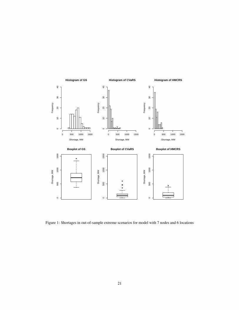
In this section, we conduct an out-of-sample analysis of the constructed wind farm location models. To thisend, we consider optimal solutions of the risk-neutral and risk-averse problems (GS, CVaRS, and HMCRS,respectively) for given fixed sets of parameters and scenarios, and then compute appropriate quantities ofinterest (for example, power shortages) under the assumption that one of the relevant parameters of the modelassumes values that are different from those used in the corresponding optimization problem (i.e., we “test”the obtained solutions on data samples that were not used during optimization). Importantly, our out-of-sample analysis focuses on the “extreme”, or “worst-case” scenarios, in order to emphasize the effects ofrisk-aversion in the solutions of the proposed models.

5.3.1 Shortage Analysis

Specifically, we assume that the out-of-sample data is represented by power demands Dik (obviously, allparameters in the respective mathematical programming problems can be replaced with out-of-sample values;but for simplicity and clarity of interpretation of the results, in this study the out-of-sample data includes onlythe power demands).

We analyzed out-of-sample shortages across the grid,Pi .Dik �

Pj �ijQjk/C, induced by the optimal

solutions of GS, CVaRS, and HMCRS problems in the case of a model with demand 7 nodes and 6 candidatelocations and 2000 scenarios based on simulated data, as well as in the case of 14 demand nodes and 8candidate locations, both with value of parameter D 0:24. We randomly generated a dataset consistingof 2000 scenarios of consumer demand Dik from the same mixed normal distribution, and selected thescenarios with shortages beyond 0.95 sample quantile in our out-of-sample scenario set as the “extreme”, or“worst-case” scenarios (in other words, the out-of-sample scenario set contained a total of 100 scenarios thatrepresent 5% of highest power shortage levels).

The results are presented in the shortage histograms and boxplots in Figures 1 and 2. In the case of thesmaller model with 7 demand nodes and 6 candidate locations, the boxplots of shortages indicate that bothrisk-averse models, HMCRS and CVaRS, significantly outperform the risk-neutral GS model. The CVaRSmodel has smaller 0.75 quantile value of shortages than HMCRS model, but it has larger extreme points.This observation is in accord with sensitivity analysis presented in the next section. Analysis of shortagehistograms shows that all shortages for HMCRS model are within 500 MW, and most of its shortages fall inthe range of [0, 50) MW, while the fraction of zero shortages exceeds 30%. As regards the CVaRS model,shortage has exceeded 500 MW in one scenario, but most of its shortages do not exceed 250 MW, also witha high fraction of zero shortages. In contrast, “extreme” out-of-sample power shortages in GS model arealways non-zero and fall mainly between 500 MW and 1000 MW, and can be as high as 1500 MW.

Similarly, in the case of models with 14 demand nodes and 8 candidate locations, boxplots in Figure 2 indicatethat the HMCRS model has the lowest 0.25 quantile, median, 0.75 quantile, etc., and CVaRS model performsmuch better than the GS model. The histograms of power shortages indicate that over 20% of out-of-sampleshortages are within Œ0; 250/MW for HMCRS model. However, no shortages fall into this range in the case ofCVaRS and GS models. Also, 98% of “extreme” out-of-sample shortages are below 1000 MW for HMCRSmodel. Although over 70% of “extreme” out-of-sample shortages are under 1000 MW for CVaRS model,there is a substantial number of out-of-sample shortages within [1000,1500) MW, and even reaching 2000MW in one scenario. As regards the GS model, most of its shortages are between 1000 MW and 2000 MW,and it has nearly 5% of “extreme” out-of-sample shortages beyond 2000 MW. The largest shortage that wasobserved in the GS model is close to 2500 MW.

5.3.2 Sensitivity with Respect to Shortage Penalty Parameter

Recall that the sensitivity to power shortages of the risk-averse CVaRS and HMCRS models is determinedby the parameter , which represents the dollar cost of 1 MW of power short. The risk-neutral GS model is

20

Histogram of GS

Shortage, MW

Fre

quen

cy

0 500 1000 1500

010

2030

40

Histogram of CVaRS

Shortage, MW

Fre

quen

cy

0 500 1000 1500

010

2030

40

Histogram of HMCRS

Shortage, MW

Fre

quen

cy

0 500 1000 1500

010

2030

40

●

050

010

0015

00

Boxplot of GS

Sho

rtag

e, M

W

●

●

●

●

050

010

0015

00

Boxplot of CVaRS

Sho

rtag

e, M

W

●

050

010

0015

00Boxplot of HMCRS

Sho

rtag

e, M

W

Figure 1: Shortages in out-of-sample extreme scenarios for model with 7 nodes and 6 locations

21

Histogram of GS

Shortage, MW

Fre

quen

cy

0 500 1500 2500

05

1015

2025

30

Histogram of CVaRS

Shortage, MW

Fre

quen

cy

0 500 1500 2500

05

1015

2025

30

Histogram of HMCRS

Shortage, MW

Fre

quen

cy

0 500 1500 2500

05

1015

2025

30

●

050

010

0015

0020

0025

00

Boxplot of GS

Sho

rtag

e, M

W

●

050

010

0015

0020

0025

00

Boxplot of CVaRS

Sho

rtag

e, M

W

●

●

050

010

0015

0020

0025

00Boxplot of HMCRS

Sho

rtag

e, M

W

Figure 2: Shortages in out-of-sample extreme scenarios for model with 14 nodes and 8 locations

22

insensitive to (does not contain) the parameter , and, moreover, for the value of D 0, all three models yieldthe same solutions. In this section, we evaluate several aspects of the performance of the GS, CVaRS, andHMCRS models with respect to different levels of sensitivity to power shortages, corresponding to varyingthe value of the parameter from 0 to 0.95. Obviously, the solution of the GS model would not change with , and can be considered as the “reference” point in this comparison.

To evaluate the performance of three models, we consider four criteria: (1) the amortized annual cost, (2)the mean cumulative shortage across the grid, (3) the number of shortage scenarios, i.e., the scenarios underwhich shortages occur, and (4) the mean number of demand nodes that experience shortages. The annual costis computed as

Pj fjxj C

Pi

Pj cj �ij C

Pi

Pj �dijyij ; according to Section 5.3, the cumulative shortage

at scenario k is defined asPi .Dik �

Pj �ijQjk/C, and thus mean shortage is EŒ

Pi .Dik �

Pj �ijQjk/C�.

As in the previous section, the out-of-sample analysis is conducted, in the sense that all the four criteriaare evaluated on the set of 100 “extreme” out-of-sample scenarios determined as described above, e.g., themean shortage and the mean number of demand nodes with shortages should be interpreted as a conditionalexpectations. The four criteria are thus computed for the case of 7 demand nodes and 6 candidate locationsand 2,000 scenarios, and values of varying from 0 to 0.95 with a step of 0.05. The results are presented inFigure 3, where the horizontal (constant) lines correspond to the GS model.

0.0 0.2 0.4 0.6 0.8

300

350

400

450

500

Gamma

Cos

t

GSCVaRSHMCRS

0.0 0.2 0.4 0.6 0.8

020

040

060

0

Gamma

Mea

n S

hort

age

GSCVaRSHMCRS

0.0 0.2 0.4 0.6 0.8

020

4060

8010

0

Gamma

No.

of S

hort

age

Sce

nario

s

GSCVaRSHMCRS

0.0 0.2 0.4 0.6 0.8

01

23

45

6

Gamma

Mea

n N

o. o

f Sho

rtag

e N

odes

GSCVaRSHMCRS

Figure 3: Out-of-sample performance of GS, CVaRS and HMCRS with regard to

As expected, the annual costs of CVaRS and HMCRS models increase with . In contrast, mean shortage andmean number of shortage nodes in the CVaRS and HMCRS models decrease sharply with . Compared with

23

the CVaRS model, the HMCRS model always performs better in terms of criteria (2)–(4), except for values around 0.5, but incurs higher annual costs. In conclusion, CVaRS and HMCRS models could be tuned tofit user’s risk-averse preference so as to achieve better risk control of power shortages.

6 Conclusions

In this paper, we have considered three different stochastic optimization models for strategic wind farmlocation and operation: a risk-neutral model, a two models where risk preferences are represented by alinear risk measure (Conditional Value-at-Risk), and a nonlinear risk measure (Higher-Moment CoherentRisk measure). We proposed a branch-and-bound algorithm based on Benders decomposition technique tosolve the resulting linear and p-order cone mixed-integer programming problems. The conducted numericalstudy demonstrates the efficiency of developed algorithms, and also indicates the risk-averse models allowfor drastic reduction of wind power shortages, and can effectively be used in strategic location and planningproblems.

Acknowledgments

This work was supported in part by the DTRA grant HDTRA1-14-1-0065 and NSF grant DMI 0457473.

References[1] Abbey, C. and Joos, G. (2009) “A stochastic optimization approach to rating of energy storage systems in wind-

diesel isolated grids,” Power Systems, IEEE Transactions on, 24 (1), 418–426.

[2] Aksoy, H., Toprak, Z. F., Aytek, A., and Unal, N. E. (2004) “Stochastic generation of hourly mean wind speed data,”Renewable energy, 29 (14), 2111–2131.

[3] Artzner, P., Delbaen, F., Eber, J.-M., and Heath, D. (1999) “Coherent measures of risk,” Mathematical finance, 9 (3),203–228.

[4] Azaron, A., Brown, K., Tarim, S., and Modarres, M. (2008) “A multi-objective stochastic programming approachfor supply chain design considering risk,” International Journal of Production Economics, 116 (1), 129–138.

[5] Baghalian, A., Rezapour, S., and Farahani, R. Z. (2013) “Robust supply chain network design with service levelagainst disruptions and demand uncertainties: A real-life case,” European Journal of Operational Research, 227 (1),199–215.

[6] Baron, O., Milner, J., and Naseraldin, H. (2011) “Facility location: A robust optimization approach,” Productionand Operations Management, 20 (5), 772–785.

[7] Ben-Tal, A. and Nemirovski, A. (2001) Lectures on modern convex optimization: analysis, algorithms, and engi-neering applications, volume 2 of MPS/SIAM Series on Optimization, SIAM.

[8] Ben-Tal, A. and Nemirovski, A. (2001) “On polyhedral approximations of the second-order cone,” Mathematics ofOperations Research, 26 (2), 193–205.

[9] Benders, J. F. (1962) “Partitioning procedures for solving mixed-variables programming problems,” Numerischemathematik, 4 (1), 238–252.

[10] Berman, O. and Drezner, Z. (2008) “The p-median problem under uncertainty,” European Journal of OperationalResearch, 189 (1), 19–30.

[11] Berman, O., Krass, D., and Menezes, M. B. (2007) “Facility reliability issues in network p-median problems:strategic centralization and co-location effects,” Operations Research, 55 (2), 332–350.

24

[12] Birge, J. R. and Louveaux, F. (2011) Introduction to Stochastic Programming, Springer, New York, 2nd edition.

[13] Burke, D. J. and O’Malley, M. (2008) “Optimal wind power location on transmission systems-a probabilistic loadflow approach,” in: “Probabilistic Methods Applied to Power Systems, 2008. PMAPS’08. Proceedings of the 10thInternational Conference on,” 1–8, IEEE.

[14] Burton, T., Jenkins, N., Sharpe, D., and Bossanyi, E. (2011) Wind energy handbook, John Wiley & Sons.

[15] Carpentier, J. (1962) “Contribution a letude du dispatching economique,” Bulletin de la Societe Francaise desElectriciens, 3 (1), 431–447.

[16] Chen, G., Daskin, M. S., Shen, Z.-J. M., and Uryasev, S. (2006) “The ˛-reliable mean-excess regret model forstochastic facility location modeling,” Naval Research Logistics (NRL), 53 (7), 617–626.

[17] Clauset, A., Shalizi, C. R., and Newman, M. E. (2009) “Power-law distributions in empirical data,” SIAM review,51 (4), 661–703.

[18] Conserve Energy Future (2013) “Cost of Wind Energy,” http://www.conserve-energy-future.com/WindEnergyCost.php, [Online; accessed 12-Nov-2013].

[19] Cui, T., Ouyang, Y., and Shen, Z.-J. M. (2010) “Reliable facility location design under the risk of disruptions,”Operations Research, 58 (4-part-1), 998–1011.

[20] Daskin, M. S., Hesse, S. M., and Revelle, C. S. (1997) “˛-reliable p-minimax regret: A new model for strategicfacility location modeling,” Location Science, 5 (4), 227–246.

[21] Dommel, H. W. and Tinney, W. F. (1968) “Optimal power flow solutions,” IEEE transactions on power apparatusand systems, (10), 1866–1876.

[22] Drezner, Z. (1987) “Heuristic solution methods for two location problems with unreliable facilities,” Journal of theOperational Research Society, 509–514.

[23] Ekren, O. and Ekren, B. Y. (2010) “Size optimization of a PV/wind hybrid energy conversion system with batterystorage using simulated annealing,” Applied Energy, 87 (2), 592–598.

[24] Garcia, A., Torres, J., Prieto, E., and De Francisco, A. (1998) “Fitting wind speed distributions: a case study,” SolarEnergy, 62 (2), 139–144.

[25] Ghiani, G., Laporte, G., and Musmanno, R. (2004) Introduction to logistics systems planning and control, JohnWiley & Sons, New York.

[26] Glass, R., Beyeler, W., Stamber, K., Glass, L., LaViolette, R., Conrad, S., Brodsky, N., Brown, T., Scholand, A.,and Ehlen, M. (2005) “Simulation and Analysis of Cascading Failure in Critical Infrastructure,” Technical report,Sandia National Laboratories.

[27] Katsigiannis, Y. and Georgilakis, P. (2008) “Optimal sizing of small isolated hybrid power systems using tabusearch,” Journal of Optoelectronics and Advanced Materials, 10 (5), 1241.

[28] Kouvelis, P. and Yu, G. (1997) Robust discrete optimization and its applications, Kluwer Academic Publishers,Dordrecht.

[29] Krokhmal, P., Zabarankin, M., and Uryasev, S. (2011) “Modeling and optimization of risk,” Surveys in OperationsResearch and Management Science, 16 (2), 49–66.

[30] Krokhmal, P. A. (2007) “Higher moment coherent risk measures,” Quantitative Finance, 7 (4), 373–387.

[31] Krokhmal, P. A. and Soberanis, P. (2010) “Risk optimization with p-order conic constraints: A linear programmingapproach,” European Journal of Operational Research, 201 (3), 653–671.

[32] Kuznia, L., Zeng, B., Centeno, G., and Miao, Z. (2011) “Stochastic optimization for power system configurationwith renewable energy in remote areas,” Annals of Operations Research, 1–22.

[33] Lopez, A., Roberts, B., Heimiller, D., Blair, N., and Porro, G. (2012) “U.S. renewable energy technical potentials:a GIS-based analysis,” Technical report, National Renewable Energy Laboratory.

25

[34] Louveaux, F. (1986) “Discrete stochastic location models,” Annals of Operations research, 6 (2), 21–34.

[35] Lu, M., Ran, L., and Shen, Z.-J. M. (2015) “Reliable Facility Location Design Under Uncertain Correlated Disrup-tions,” Manufacturing & Service Operations Management, 17 (4), 445–455.

[36] Mei, S., Zhang, X., and Cao, M. (2011) Power grid complexity, Springer.

[37] Melo, M. T., Nickel, S., and Saldanha-Da-Gama, F. (2009) “Facility location and supply chain management–Areview,” European journal of operational research, 196 (2), 401–412.

[38] Mirchandani, P. B. and Oudjit, A. (1980) “Localizing 2-medians on probabilistic and deterministic tree networks,”Networks, 10 (4), 329–350.

[39] Mirchandani, P. B., Oudjit, A., and Wong, R. T. (1985) “‘Multidimensional’ extensions and a nested dual approachfor the m-median problem,” European Journal of Operational Research, 21 (1), 121–137.

[40] Morenko, Y., Vinel, A., Yu, Z., and Krokhmal, P. (2013) “On p-cone linear discrimination,” European Journal ofOperational Research, 231, 784–789.

[41] Nesterov, Y., Nemirovskii, A., and Ye, Y. (1994) Interior-point polynomial algorithms in convex programming,volume 13 of Studies in Applied Mathematics, SIAM, Philadelphia, PA.

[42] Owen, S. H. and Daskin, M. S. (1998) “Strategic facility location: A review,” European Journal of OperationalResearch, 111 (3), 423–447.

[43] Peng, P., Snyder, L. V., Lim, A., and Liu, Z. (2011) “Reliable logistics networks design with facility disruptions,”Transportation Research Part B: Methodological, 45 (8), 1190–1211.

[44] Prekopa, A. (1995) Stochastic Programming, Kluwer Academic Publishers.

[45] Rahmaniani, R., Crainic, T. G., Gendreau, M., and Rei, W. (2017) “The Benders decomposition algorithm: Aliterature review,” European Journal of Operational Research, 259 (3), 801–817.

[46] Rockafellar, R. T. and Uryasev, S. (2000) “Optimization of conditional value-at-risk,” Journal of risk, 2, 21–42.

[47] Rockafellar, R. T. and Uryasev, S. (2002) “Conditional value-at-risk for general loss distributions,” Journal ofBanking & Finance, 26 (7), 1443–1471.

[48] Roques, F., Hiroux, C., and Saguan, M. (2010) “Optimal wind power deployment in Europea portfolio approach,”Energy Policy, 38 (7), 3245–3256.

[49] Santoso, T., Ahmed, S., Goetschalckx, M., and Shapiro, A. (2005) “A stochastic programming approach for supplychain network design under uncertainty,” European Journal of Operational Research, 167 (1), 96–115.

[50] Schutz, P., Tomasgard, A., and Ahmed, S. (2009) “Supply chain design under uncertainty using sample averageapproximation and dual decomposition,” European Journal of Operational Research, 199 (2), 409–419.

[51] Schwartz, M., Heimiller, D., Haymes, S., and Walt, M. (2010) “Assessment of offshore wind energy resources forthe United States,” Technical report, National Renewable Energy Laboratory.

[52] Scott, W. R. and Powell, W. B. (2012) “Approximate dynamic programming for energy storage with new results oninstrumental variables and projected Bellman errors,” Submitted to Operations Research (Under Review).

[53] Senjyu, T., Hayashi, D., Yona, A., Urasaki, N., and Funabashi, T. (2007) “Optimal configuration of power generatingsystems in isolated island with renewable energy,” Renewable Energy, 32 (11), 1917–1933.

[54] Shapiro, A., Dentcheva, D., and Ruszczynski, A. (2009) Lectures on Stochastic Programming: Modeling andTheory, SIAM-MPS, Philadelphia.

[55] Shapiro, J. F. (2001) Modeling the Supply Chain, Duxbury Press, Pacific Grove, CA.

[56] Shen, Z.-J. M., Zhan, R. L., and Zhang, J. (2011) “The reliable facility location problem: Formulations, heuristics,and approximation algorithms,” INFORMS Journal on Computing, 23 (3), 470–482.

26

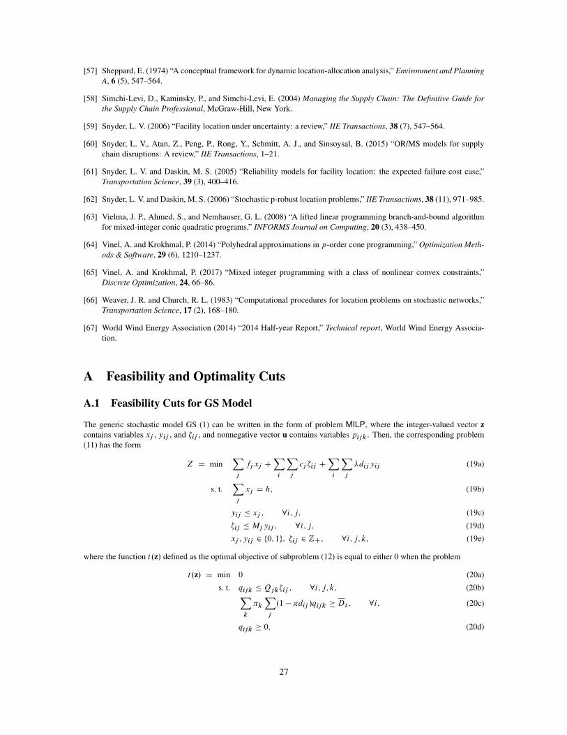
[57] Sheppard, E. (1974) “A conceptual framework for dynamic location-allocation analysis,” Environment and PlanningA, 6 (5), 547–564.

[58] Simchi-Levi, D., Kaminsky, P., and Simchi-Levi, E. (2004) Managing the Supply Chain: The Definitive Guide forthe Supply Chain Professional, McGraw-Hill, New York.

[59] Snyder, L. V. (2006) “Facility location under uncertainty: a review,” IIE Transactions, 38 (7), 547–564.

[60] Snyder, L. V., Atan, Z., Peng, P., Rong, Y., Schmitt, A. J., and Sinsoysal, B. (2015) “OR/MS models for supplychain disruptions: A review,” IIE Transactions, 1–21.

[61] Snyder, L. V. and Daskin, M. S. (2005) “Reliability models for facility location: the expected failure cost case,”Transportation Science, 39 (3), 400–416.

[62] Snyder, L. V. and Daskin, M. S. (2006) “Stochastic p-robust location problems,” IIE Transactions, 38 (11), 971–985.

[63] Vielma, J. P., Ahmed, S., and Nemhauser, G. L. (2008) “A lifted linear programming branch-and-bound algorithmfor mixed-integer conic quadratic programs,” INFORMS Journal on Computing, 20 (3), 438–450.

[64] Vinel, A. and Krokhmal, P. (2014) “Polyhedral approximations in p-order cone programming,” Optimization Meth-ods & Software, 29 (6), 1210–1237.

[65] Vinel, A. and Krokhmal, P. (2017) “Mixed integer programming with a class of nonlinear convex constraints,”Discrete Optimization, 24, 66–86.

[66] Weaver, J. R. and Church, R. L. (1983) “Computational procedures for location problems on stochastic networks,”Transportation Science, 17 (2), 168–180.

[67] World Wind Energy Association (2014) “2014 Half-year Report,” Technical report, World Wind Energy Associa-tion.

A Feasibility and Optimality Cuts

A.1 Feasibility Cuts for GS Model

The generic stochastic model GS (1) can be written in the form of problem MILP, where the integer-valued vector zcontains variables xj , yij , and �ij , and nonnegative vector u contains variables pijk . Then, the corresponding problem(11) has the form

Z D minXj

fj xj CXi

Xj

cj �ij CXi

Xj

�dij yij (19a)

s. t.Xj

xj D h; (19b)

yij � xj ; 8i; j; (19c)

�ij �Mj yij ; 8i; j; (19d)

xj ; yij 2 f0; 1g; �ij 2 ZC; 8i; j; k; (19e)

where the function t .z/ defined as the optimal objective of subproblem (12) is equal to either 0 when the problem

t .z/ D min 0 (20a)

s. t. qijk � Qjk�ij ; 8i; j; k; (20b)Xk

�k

Xj

.1 � ~dij /qijk � Di ; 8i; (20c)

qijk � 0; (20d)

27

is feasible for the given values of �ij , or t .z/ D C1when (20) is infeasible. Obviously, if Oz D . Oxj ; Oyij ; O�ij / is an optimalsolution of (19) such that (20) has a feasible Oqijk for the given O�ij , then .Oz; Ou/ D . Oxj ; Oyij ; O�ij ; Oqijk/ is an optimal solutionof the original problem (1). On the other hand, if (20) is infeasible, then the corresponding Oz should be eliminated fromthe feasible region of the master problem (19). In accordance to the described above algorithm, this is accomplished byaugmenting (19) with feasibility cuts X

i

Xj

Xk

Qjk O ijk�ij �Xi

Di Oi � 0; (21)

where . O ijk ; Oi / is an extreme ray of the dual SMILP.Oz/ of problem (20), which takes the form

t .Oz/ D maxXi

Xj

Xk

QjkO�ij ˛ijk �

Xi

Diˇi (22a)

s. t. ˛ijk � �k.1 � ~dij /ˇi � 0; 8i; j; k; (22b)

˛ijk ; ˇi � 0; 8i; j; k: (22c)

Clearly, no optimality cuts are added to (19) since (20) is a “feasibility” subproblem.

A.2 Feasibility and Optimality Cuts for CVaRS Model

Analogously to above, the CVaRS model (8) can be reformulated in the form (11)–(12) as follows

Z D minXj

fj xj CXi

Xj

cj �ij CXi

Xj

�dij yij C t (23a)

s. t.Xj

xj D h; (23b)

yij � xj ; 8i; j; (23c)

�ij �Mj yij ; 8i; j; (23d)

xj ; yij 2 f0; 1g; �ij 2 ZC; t 2 R; (23e)

with the subproblem (20) defined as:

t .Oz/ D min �C1

1 � ˛

Xk

�kUk (24a)

s. t. qijk � QjkO�ij ; 8i; j; k; (24b)X

k

�k

Xj

.1 � ~dij /qijk � Di ; 8i; (24c)

wik � Dik �Xj

qijk ; 8i; k; (24d)

Uk �Xi

wik � �; 8k; (24e)

wik ; qijk ; Uk � 0; 8i; j; k: (24f)

Let ˛ijk , �i , ˇik , and �k be the dual variables associated with constraints (24b), (24c), (24d) and (24e) respectively.Then, the dual of subproblem becomes

t .z/ D maxXi

Xj

Xk

QjkO�ij ˛ijk �

Xi

Xk

Dikˇik �Xi

Di�i (25a)

s. t. ˛ijk � ˇik � �k.1 � ~dij /�i � 0; 8i; j; k; (25b)

� �k �1

1 � ˛�k ; 8k; (25c)

� ˇik C �k � 0; 8i; k; (25d)

28

�

Xk

�k � 1; (25e)

˛ijk ; �i ; ˇik ; �k � 0; 8i; j; k: (25f)

If, for a given set of values O�ij , where . Oxj ; Oyij ; O�ij ; Ot / is an optimal solution of (23), problem (25) is unbounded, let. O ijk ;

Oik ; O�i / be an extreme ray of the feasible region of (25), such that

Pi

Pj

Pk .Qjk O ijk/

O�ij �Pi

Pk Dik

Oik�P

i Di O�i > 0. Then, the feasibility cutXi

Xj

Xk

Qjk O ijk�ij �Xi

Xk

DikOik �

Xi

Di O�i � 0; (26)

is added to the master problem. If, on the other hand, the optimal objective t� D t .Oz/ of (25) is finite and such thatOt < t�, the following optimality cut is added to the master:X

i

Xj

Xk

Qjk O ijk�ij �Xi

Xk

DikOik �

Xi

Di O�i � t; (27)

where . O ijk ; Oik ; O�i / is an optimal solution of (25).

A.3 Feasibility and Optimality Cuts for HMCRS Model

The polyhedral approximation of the HMCRS model (10) can be written in the form of a mixed-integer linear problemMILP where, as before, the integer-valued vector z comprises variables xj , yij , and �ij , so that the correspondingproblem (11) has the form

Z D minXj

fj xj CXi

Xj

cj �ij CXi

Xj

�dij yij C t (28a)

s. t.Xj

xj D h; (28b)

yij � xj ; 8i; j; (28c)

�ij �Mj yij ; 8i; j; (28d)

xj ; yij 2 f0; 1g; �ij 2 ZC; t � 0; (28e)

and the subproblem (12), whose optimal objective t .z/ defines the value of variable t above, takes the form

t .z/ D min �C .1 � ˛/�1U2K�1 (29a)

s. t. qijk � Qjk�ij ; 8i; j; n; (29b)Xk

�k

Xj

.1 � ~dij /qijk � Di ; 8i; (29c)

wik � Dik �Xj

qijk ; 8i; k; (29d)

Uk � �1=pk

�Xi

wik � �

�; 8k; (29e)

UKCr � a.p/lU2r�1 C b

.p/lU2r ; 8r; l; k (29f)

wik ; qijk ; Uk � 0; (29g)

where the nonnegative variables pijk , wik , and Uk comprise the vector u, see (12).

Let ˛ijk , �i , ˇik , �k , and �lk be the multipliers associated with constraints (29b), (29c), (29d), (29e), and (29f), respec-tively. Then, the dual of subproblem (29) can be written as

t .z/ D maxXi

Xj

Xk

Qjk�ij ˛ijk �Xi

Xk

Dikˇik �Xi

Di�i (30a)

s. t. ˛ijk � ˇik � �k.1 � ~dij /�i � 0; 8i; j; k; (30b)

29

� ˇik C �k � 0; 8i; k; (30c)

�

Xk

�k � 1; (30d)

� �k CXl

a.p/l�ld k2 e

� 0; 8k D 1; 3; : : : ; K � 1; (30e)

� �k CXl

b.p/l�ld k2 e

� 0; 8k D 2; 4; : : : ; K; (30f)

Xl

A.p/l�l.K2 Cd

k2 e/�

Xl

�lk � 0; 8k D 1; 3; : : : ; K � 3; (30g)

Xl

B.p/l�l.K2 Cd

k2 e/�

Xl

�lk � 0; 8k D 2; 4; : : : ; K � 2; (30h)

�

Xl

�l.K�1/ �1

1 � ˛; (30i)

˛ijk ; �i ; ˇik ; �k ; �lk � 0: (30j)

For the sake of simplicity, we assume K is an even number. If, for a given optimal value Oz obtained from (28), problem(30) is unbounded, let . O ; O ; O�/ be an extreme ray of (30), such that

Pi

Pj

Pk Qjk O ijk

O�ij �Pi

Pk Dik

Oik �P

i Di O�i > 0. Then, a feasibility cutXi

Xj

Xk

Qjk O ijk�ij �Xi

Xk

DikOik �

Xi

Di O�i � 0; (31)

is added to (28). Conversely, let Ot and t� denote an optimal value of t in the master problem (28), and the optimalobjective function value of problem (30), respectively. If Ot < t�, then an optimality cutX

i

Xj

Xk

Qjk O ijk�ij �Xi

Xk

DikOik �

Xi

Di O�i � t; (32)

is added to the master problem (28).

30