Risk Assessment Technical Background Document for the ...

Risk Assessment

Technical Background Document for

the Chlorinated Aliphatics Listing Determination

Addendum

September 29, 2000

USEPA Office of Solid Waste

Economics, Methods, and Risk Analysis Division

iii

TABLE OF CONTENTS

1. INTRODUCTION . . . . . . . . . . . . . . . . . . . . . . . . . . . . . . . . . . . . . . . . . . . . . . . . . . . . . . . 1-1

2. ESTABLISHING CONTAMINANT EXPOSURE SCENARIOS . . . . . . . . . . . . . . . . . . . . . 2-12.1 Support for EPA’s Assumptions Regarding the Plausibility of Beef and Dairy

Cattle Farming in the Vicinity of Chlorinated Aliphatics Facilities . . . . . . . . . . 2-12.2 Evaluation of EPA’s Assumptions Regarding the Modeled Pasture Size . . . . 2-32.3 Evaluation of the Exposure Scenario as it Relates to the Probabilistic

Analyses . . . . . . . . . . . . . . . . . . . . . . . . . . . . . . . . . . . . . . . . . . . . . . . . . . . 2-25

3. ESTIMATING EXPOSURE POINT CONCENTRATIONS . . . . . . . . . . . . . . . . . . . . . . . . 3-13.1 Removal of Solids from Wastewater Prior to Aerated Biological Treatment . . 3-13.2 Mass Balance Correction for the Land Treatment Unit Erosion Pathway

Analysis . . . . . . . . . . . . . . . . . . . . . . . . . . . . . . . . . . . . . . . . . . . . . . . . . . . . 3-8

4. EXPOSURE AND TOXICITY ASSESSMENTS . . . . . . . . . . . . . . . . . . . . . . . . . . . . . . . . 4-14.1 Cooking and Post-Cooking Loss of Beef . . . . . . . . . . . . . . . . . . . . . . . . . . . . 4-14.2 Chloroform Exposure Point Concentrations and Toxicity Assessment . . . . . . 4-3

5. RISK CHARACTERIZATION . . . . . . . . . . . . . . . . . . . . . . . . . . . . . . . . . . . . . . . . . . . . . . 5-15.1 Non-Cancer Health Effects Resulting from Exposure to Dioxins and

Evaluation of Dioxin Exposure for Nursing Infants . . . . . . . . . . . . . . . . . . . . . 5-15.2 Pathway and Exposure Route-Specific Land Treatment Unit TCDD TEQ Risk

Estimates for the Adult Farmer . . . . . . . . . . . . . . . . . . . . . . . . . . . . . . . . . . . 5-55.3 Summary of High End Risk Estimates – Chlorinated Aliphatics Wastewaters

and EDC/VCM Sludges . . . . . . . . . . . . . . . . . . . . . . . . . . . . . . . . . . . . . . . . . 5-75.4 Population Risk Estimates . . . . . . . . . . . . . . . . . . . . . . . . . . . . . . . . . . . . . . 5-11

6. REFERENCES . . . . . . . . . . . . . . . . . . . . . . . . . . . . . . . . . . . . . . . . . . . . . . . . . . . . . . . . . 6-1

7. APPENDICES . . . . . . . . . . . . . . . . . . . . . . . . . . . . . . . . . . . . . . . . . . . . . . . . . . . . . . . . . 7-1

8. ERRATA . . . . . . . . . . . . . . . . . . . . . . . . . . . . . . . . . . . . . . . . . . . . . . . . . . . . . . . . . . . . . 8-1

iv

LIST OF TABLES

Table 2-1. Presence of Beef Cattle and Dairy Cows in Counties Where ChlorinatedAliphatics Production Facilities are Located . . . . . . . . . . . . . . . . . . . . . . . . . 2-2

Table 2-2. Distance of Receptor Points from Source and Distance between Receptors– Tank . . . . . . . . . . . . . . . . . . . . . . . . . . . . . . . . . . . . . . . . . . . . . . . . . . . . . 2-11

Table 2-3. Distance of Receptor Points from Source and Distance between Receptors– Land Treatment Unit . . . . . . . . . . . . . . . . . . . . . . . . . . . . . . . . . . . . . . . . . 2-11

Table 2-4. Tank, Memphis, TN - Unitized Air Concentrations . . . . . . . . . . . . . . . . . . . . 2-14Table 2-5. Land Treatment Unit, Baton Rouge, LA - Unitized Air Concentrations . . . . . 2-16Table 2-6. Calculation of Average Concentration Over 275m by 275m Pasture – Tank 2-23Table 2-7. Calculation of Average Concentration Over 275m by 275m Pasture – Land

Treatment Unit . . . . . . . . . . . . . . . . . . . . . . . . . . . . . . . . . . . . . . . . . . . . . . . 2-24

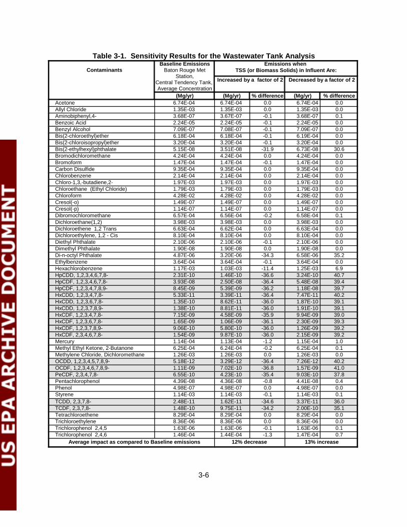
Table 3-1. Sensitivity Results for the Wastewater Tank Analysis . . . . . . . . . . . . . . . . . . 3-6Table 3-2. Ratio of the 1999 High End Emissions Estimate and Emissions Estimate that

Assumes Solids (TSS) Removal Prior to Aerated Biological Treatment – 70%TSS Removal Efficiency . . . . . . . . . . . . . . . . . . . . . . . . . . . . . . . . . . . . 3-7

Table 3-3. Ratio of the 1999 High End Emissions Estimate and Emissions Estimate thatAssumes Solids (TSS) Removal Prior to Aerated Biological Treatment – 50%TSS Removal Efficiency . . . . . . . . . . . . . . . . . . . . . . . . . . . . . . . . . . . . . . . . . 3-7

Table 3-4. Erosion Mass Balance Calculation – Land Treatment Unit (LTU) . . . . . . . . . 3-10Table 3-5. Central Tendency TCDD TEQ Emission Estimates for the EDC/VCM Land

Treatment Unit . . . . . . . . . . . . . . . . . . . . . . . . . . . . . . . . . . . . . . . . . . . . . . . 3-11Table 3-6. High End TCDD TEQ Emission Estimates for the EDC/VCM Land

Treatment Unit . . . . . . . . . . . . . . . . . . . . . . . . . . . . . . . . . . . . . . . . . . . . . . . 3-12

Table 4-1. Chloroform Exposure Point Concentrations in Air . . . . . . . . . . . . . . . . . . . . . 4-6

Table 5-1. TCDD TEQ Risk Results for the Adult Farmer, Land Treatment Unit . . . . . . . 5-6Table 5-2. Modifications to the High End Deterministic Risk Estimate (TCDD TEQ)

for the Adult Farmer – Chlorinated Aliphatics Wastewaters . . . . . . . . . . . . . . 5-8Table 5-3. Modifications to the High End Deterministic Risk Estimate (TCDD TEQ)

for the Adult Farmer – EDC/VCM Sludges Managed in a Land TreatmentUnit . . . . . . . . . . . . . . . . . . . . . . . . . . . . . . . . . . . . . . . . . . . . . . . . . . . . . . . . 5-9

v

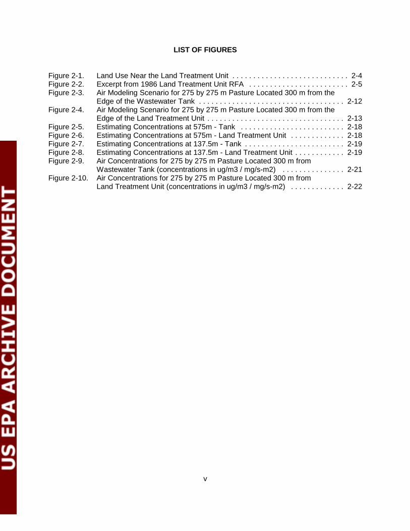
LIST OF FIGURES

Figure 2-1. Land Use Near the Land Treatment Unit . . . . . . . . . . . . . . . . . . . . . . . . . . . . 2-4Figure 2-2. Excerpt from 1986 Land Treatment Unit RFA . . . . . . . . . . . . . . . . . . . . . . . . 2-5Figure 2-3. Air Modeling Scenario for 275 by 275 m Pasture Located 300 m from the

Edge of the Wastewater Tank . . . . . . . . . . . . . . . . . . . . . . . . . . . . . . . . . . . 2-12Figure 2-4. Air Modeling Scenario for 275 by 275 m Pasture Located 300 m from the

Edge of the Land Treatment Unit . . . . . . . . . . . . . . . . . . . . . . . . . . . . . . . . . 2-13Figure 2-5. Estimating Concentrations at 575m - Tank . . . . . . . . . . . . . . . . . . . . . . . . . 2-18Figure 2-6. Estimating Concentrations at 575m - Land Treatment Unit . . . . . . . . . . . . . 2-18Figure 2-7. Estimating Concentrations at 137.5m - Tank . . . . . . . . . . . . . . . . . . . . . . . . 2-19Figure 2-8. Estimating Concentrations at 137.5m - Land Treatment Unit . . . . . . . . . . . . 2-19Figure 2-9. Air Concentrations for 275 by 275 m Pasture Located 300 m from

Wastewater Tank (concentrations in ug/m3 / mg/s-m2) . . . . . . . . . . . . . . . 2-21Figure 2-10. Air Concentrations for 275 by 275 m Pasture Located 300 m from

Land Treatment Unit (concentrations in ug/m3 / mg/s-m2) . . . . . . . . . . . . . 2-22

September 29, 2000

1The terminology used in this document is the same as that used in the 1999 RiskAssessment TBD and is not redefined in this Addendum.

1-1

1. INTRODUCTION

On August 25, 1999, the Environmental Protection Agency (EPA) published a proposed

rulemaking for wastewaters and wastewater treatment sludges from the production of

chlorinated aliphatic chemicals. In conjunction with this proposed rulemaking EPA prepared a

“Risk Assessment Technical Background Document for the Chlorinated Aliphatics Listing

Determination” (with attached Addendum) dated July 30, 1999 (“1999 Risk Assessment TBD”;

USEPA 1999).

The purpose of this 2000 Addendum is 1) to provide information that EPA prepared in

response to public and peer review comment on the proposed rulemaking that modifies,

clarifies, or supplements information we presented in the 1999 Risk Assessment TBD and 2) to

present a list of errata for the 1999 Risk Assessment TBD. This supplemental background

document is intended as a companion to the 1999 Risk Assessment TBD, and is not intended

to be a stand-alone document1. Sections 2 through 6 of this Addendum generally correspond

to Sections 2 through 6 of the 1999 Risk Assessment TBD, and discuss issues by the following

topic areas:

• Establishing contaminant exposure scenarios (Section 2)

• Estimating exposure point concentrations (Section 3)

• Exposure and toxicity assessments (Section 4)

• Risk characterization (Section 5)

Section 6 provides references for this addendum. Section 7 provides new versions of

Appendices D.1, D.2, D.4, D.5, and F.1 that have been modified in response to peer review

comments. Section 8 provides a list of errata for the 1999 Risk Assessment TBD.

September 29, 2000

2-1

2. ESTABLISHING CONTAMINANT EXPOSURE SCENARIOS

This section provides technical information that supplements that provided in Section 2 of

the 1999 Risk Assessment TBD. Section 2 of the background document discussed how EPA

established the exposure scenarios that we evaluated in the risk assessment. An exposure

scenario describes how an individual (a receptor) may come into contact with (be exposed to)

contaminants in a waste.

The information we provide in this section includes:

• Support for EPA’s assumption that beef and dairy cattle might plausibly be raised in the

vicinity of chlorinated aliphatics manufacturing facilities;

• An evaluation of our assumptions regarding the modeled pasture size; and

• A discussion of how certain exposure assumptions influence our probabilistic risk

estimates.

2.1 Support for EPA’s Assumptions Regarding the Plausibility of Beef and Dairy

Cattle Farming in the Vicinity of Chlorinated Aliphatics Facilities

Commenters on the proposed rule questioned EPA’s assumption that a farmer might

raise fruits, exposed vegetables, root vegetables, beef cattle and dairy cows in the vicinity of

chlorinated aliphatics production facilities. The commenters confirmed that it was plausible to

assume that beef cattle might be raised in the vicinity of chlorinated aliphatics facilities that

manage wastewaters; however, they questioned our assumptions regarding the presence of

dairy cattle in the parts of the country where chlorinated aliphatics facilities are located. To

respond to this concern, EPA reviewed publicly available data from the 1997 agricultural census

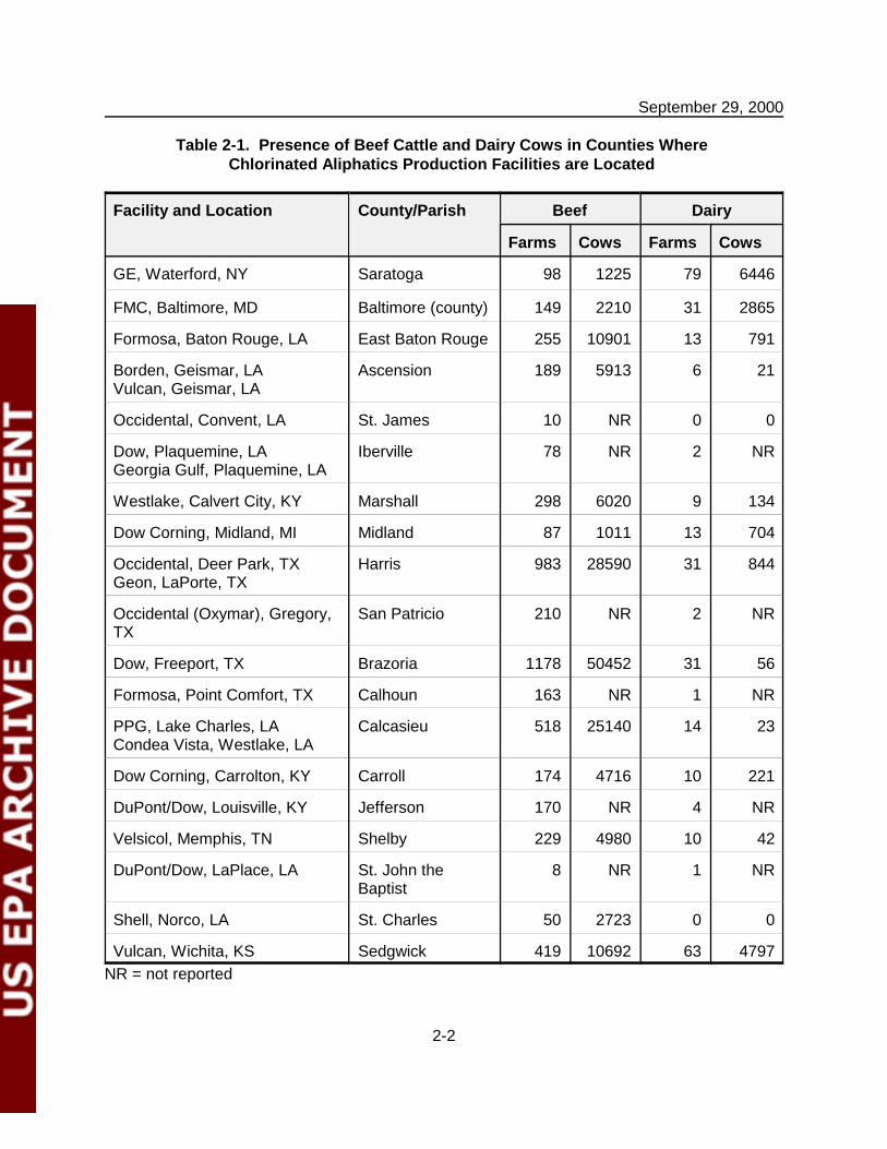
(http://govinfo.library.orst.edu/ag-stateis.html) that are summarized in Table 2-1. As shown in

Table 2-1, EPA determined that of the 23 chlorinated aliphatics production facilities,

September 29, 2000

2-2

Table 2-1. Presence of Beef Cattle and Dairy Cows in Counties WhereChlorinated Aliphatics Production Facilities are Located

Facility and Location County/Parish Beef Dairy

Farms Cows Farms Cows

GE, Waterford, NY Saratoga 98 1225 79 6446

FMC, Baltimore, MD Baltimore (county) 149 2210 31 2865

Formosa, Baton Rouge, LA East Baton Rouge 255 10901 13 791

Borden, Geismar, LAVulcan, Geismar, LA

Ascension 189 5913 6 21

Occidental, Convent, LA St. James 10 NR 0 0

Dow, Plaquemine, LAGeorgia Gulf, Plaquemine, LA

Iberville 78 NR 2 NR

Westlake, Calvert City, KY Marshall 298 6020 9 134

Dow Corning, Midland, MI Midland 87 1011 13 704

Occidental, Deer Park, TXGeon, LaPorte, TX

Harris 983 28590 31 844

Occidental (Oxymar), Gregory,TX

San Patricio 210 NR 2 NR

Dow, Freeport, TX Brazoria 1178 50452 31 56

Formosa, Point Comfort, TX Calhoun 163 NR 1 NR

PPG, Lake Charles, LACondea Vista, Westlake, LA

Calcasieu 518 25140 14 23

Dow Corning, Carrolton, KY Carroll 174 4716 10 221

DuPont/Dow, Louisville, KY Jefferson 170 NR 4 NR

Velsicol, Memphis, TN Shelby 229 4980 10 42

DuPont/Dow, LaPlace, LA St. John theBaptist

8 NR 1 NR

Shell, Norco, LA St. Charles 50 2723 0 0

Vulcan, Wichita, KS Sedgwick 419 10692 63 4797NR = not reported

September 29, 2000

2-3

21 facilities are located in counties with at least one farm that reported having dairy cows (beef

cattle were reported in all counties), confirming that ingestion of contaminated home-produced

dairy products is a plausible exposure scenario.

EPA collected additional information for the land treatment unit. First, in 1997 dairy

cattle were reported for the parish (county) in which the land treatment unit is located.

Furthermore, a land use map for the area surrounding the facility shows that cropland and

pastureland bounds the facility (Figure 2-1). Lastly, a 1986 RCRA facility Assessment Report

(RFA) confirms at least the historical proximity of cattle to waste management units at the

facility (Figure 2-2).

2.2 Evaluation of EPA’s Assumptions Regarding the Modeled Pasture Size

In the 1999 Risk Assessment Technical Background Document we presented an

analysis of risk for an adult farmer and a child of a farmer. We explained that our evaluation

considered that the farmer and his/her child resides on an agricultural farm with dimensions of

approximately 1410 meters (m) by 1410 m, and consumes fruits, exposed vegetables, and root

vegetables grown on the farm, as well as beef and dairy products produced from cattle raised

on the farm. We assumed the farm was used to provide forage, grain, and silage for the cattle.

We estimated that high end risk would exceed 1x10-5 (the hazardous waste listing program’s

target risk level) for dioxin under the aerated biological treatment tank and land treatment unit

waste management scenarios. Commenters on the proposed rule questioned the plausibility

our assumptions regarding the productivity of the farm that we evaluated. They suggested that

the exposure scenario that EPA evaluated is unrealistic in that it implies that a farm not only has

both a dairy and beef cattle operation, but raises grain and silage, in addition to crops for

human consumption, while still maintaining enough pasture to graze the animals.

September 29, 2000

2-4

Figure 2-1. Land Use Near the Land Treatment Unit

Code Land Use Description Code Land Use Description

11 Residential 41 Deciduous Forest Land

12 Commercial and Services 51 Streams and Canals

13 Industrial 76 Transitional Areas

21 Cropland and Pasture

Figure 2-2. Excerpt from 1986 Land Treatment Unit RFA

September 29, 2000

2-5

September 29, 2000

2-6

Tables 5-3 and 5-8 of the 1999 Risk Assessment Technical Background Document

show that for the adult farmer 1) 99.3 percent of the high end dioxin risk for chlorinated aliphatic

wastewaters is due to ingestion of beef and dairy products, and only 0.7 percent is due to

ingestion of home grown fruits and vegetables, and 2) 96 percent of the high end dioxin risk for

wastewater treatment sludges managed in a land treatment unit is due to ingestion of beef and

dairy products, and only 4 percent is due to ingestion of home grown fruits and vegetables. As

a result, even though EPA believes it is plausible that a subsistence or hobby farmer would

raise fruits and vegetables for home consumption, the validity of EPA’s risk estimate depends

almost entirely on the validity of our assumption that a farmer might consume both beef and

dairy products from cattle raised on a farm located in the vicinity of a chlorinated aliphatics

production facility. Moreover, under the tank scenario the dioxins in the beef and dairy products

result almost exclusively from the cattle’s intake of forage that is contaminated by air emissions

from the modeled wastewater treatment tank – negligible levels of dioxins are contributed to

cattle as a result of the cattle’s ingestion of grain, silage, or soil (see Appendix H.1, Table H.1-

1a of the 1999 Risk Assessment Technical Background Document). Similarly, under the land

treatment unit scenario the dioxins in the beef and dairy products result primarily from the

cattle’s intake of forage and soil that are contaminated by air emissions and runoff/erosion from

the modeled land treatment unit – minor levels of dioxins are contributed to cattle as a result of

the cattle’s ingestion of grain or silage (see Table 5-1). Consequently, all that is required for

the adult farmer to realize the risk that EPA presented in the proposed rule is that the farmer

consume beef and dairy products derived from cattle that consume forage and, in the case of

the land treatment unit, incidentally ingest soil, from the farmer’s pastureland/field. That is, it is

not necessary that we assume that the farmer consumes home-grown fruits and vegetables, or

that the farmer produces grain or silage for use as cattle feed.

In response to the commenters’ concerns, we reviewed our methodology for estimating

the concentrations of dioxins in forage and soil to ensure that we were adequately considering

the size of the contaminated pasture (field) versus its expected productivity. For aerated

biological treatment tanks we evaluated risks due to vapor air emissions from the tanks. For

the land treatment unit, we evaluated risks due to vapor air emissions, particulate air emissions,

and erosion/runoff emissions from the land treatment unit. In the proposed rule we explained

September 29, 2000

2-7

that in evaluating the air pathway we always assume that the cattle are located along the

centerline of the area most greatly impacted by air releases from the waste management units

(64 FR 46486). We said that for the wastewater tank analysis, the air concentrations within

about a 100-meter lateral distance from this point did not vary appreciably, and stated

specifically in our 1999 Risk Assessment Technical Background Document Addendum that the

concentrations varied about 20% within 200 meters of the point of maximum concentration. In

the course of our reevaluation of these data in response to comments, we felt that we likely

should have considered how the concentrations of dioxins in air, and therefore in forage, vary

over a wider aerial extent that would be more consistent with the area of a pasture.

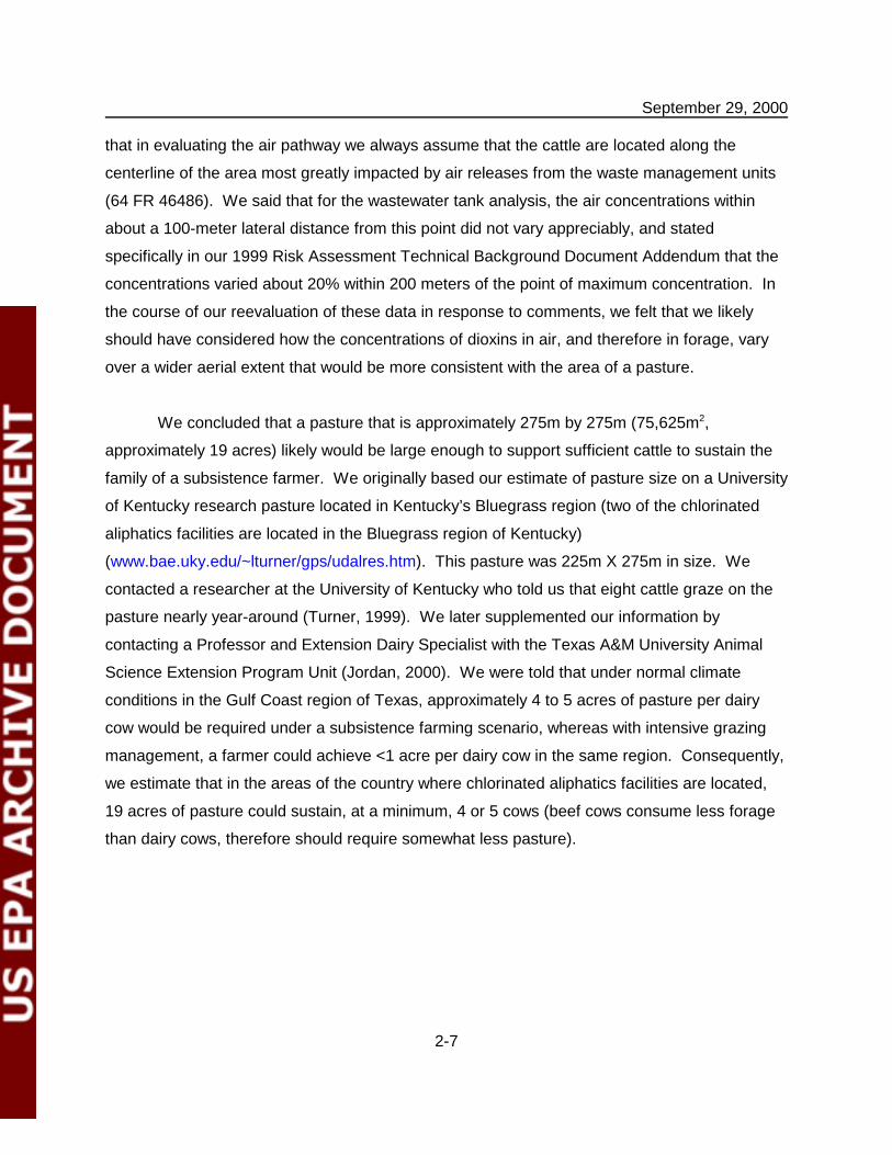
We concluded that a pasture that is approximately 275m by 275m (75,625m2,

approximately 19 acres) likely would be large enough to support sufficient cattle to sustain the

family of a subsistence farmer. We originally based our estimate of pasture size on a University

of Kentucky research pasture located in Kentucky’s Bluegrass region (two of the chlorinated

aliphatics facilities are located in the Bluegrass region of Kentucky)

(www.bae.uky.edu/~lturner/gps/udalres.htm). This pasture was 225m X 275m in size. We

contacted a researcher at the University of Kentucky who told us that eight cattle graze on the

pasture nearly year-around (Turner, 1999). We later supplemented our information by

contacting a Professor and Extension Dairy Specialist with the Texas A&M University Animal

Science Extension Program Unit (Jordan, 2000). We were told that under normal climate

conditions in the Gulf Coast region of Texas, approximately 4 to 5 acres of pasture per dairy

cow would be required under a subsistence farming scenario, whereas with intensive grazing

management, a farmer could achieve <1 acre per dairy cow in the same region. Consequently,

we estimate that in the areas of the country where chlorinated aliphatics facilities are located,

19 acres of pasture could sustain, at a minimum, 4 or 5 cows (beef cows consume less forage

than dairy cows, therefore should require somewhat less pasture).

http://www.bae.uky.edu/~lturner/gps/udalres.htm

September 29, 2000

2-8

We estimated how many cows would be necessary to sustain a family of four as follows:

Reference Dairy Beef

HE CT HE CT

Daily Consumption Rate ofDairy and Beef (pre-cooked)– Adult Farmer, kg*/day

USEPA (1999), Table K-2 2.1 0.73 0.3234 0.098

Daily Consumption of Home-Produced Dairy and Beef– Adult Farmer, kg*/day

Previous row multiplied by 0.25for dairy and 0.49 for beef(USEPA, 1999, Section 2.2.1 andTable K-2)

0.525 0.1825 0.048 0.1585

Consumption of Home-Produced Dairy and Beef forfour-person Family

kg*/daykg*/year

(Conservatively assumes that allfamily members are adults.)

Previous row multiplied by 4Previous row multiplied by 365

2.1766

0.73266

0.634231

0.19270

Average Production per Cow Dairy: Texas A&M (undated),average for Texas

Beef: USEPA (1999), Section 5.2

17 kg/day6218 kg/year

338 kg (dressedweight of 1 steer)

Number of Cows Required toSustain four-person Family

Consumption of Home-ProducedDairy/Beef Divided by AverageDairy/Beef Production per Cow

1 1 per year

* wet or fresh weight

Based on this calculation, we estimate that a farmer would require a minimum three to four

cows to sustain a family of four. One dairy cow would provide 6205 kg/year of milk, compared

to the required 766 kg/year (based on the high end consumption rate); however, two dairy cows

are necessary to ensure a continuous supply of milk (Jordan, 2000) since one or the other cow

will be dry periodically. One beef cow would provide 338 kg of beef, which is more than the

necessary 231 kg required by the family of four each year (based on the high end consumption

rate); however, a farmer likely would be raising one or two additional beef cattle for future

consumption.

We used the results of the air modeling we conducted for the proposed rulemaking to

determine the approximate difference between the air concentration that we used to calculate

the proposed risk estimate (the air concentration corresponding to a point located 300m from

the modeled wastewater treatment tank and land treatment unit) and the average air

concentration at a 75,625m2 field located 300m from the modeled wastewater treatment tank

and land treatment unit. The model we used to evaluate the erosion/runoff pathway under the

September 29, 2000

2-9

land treatment unit exposure scenario assumed that contaminants are deposited evenly across

the entire (1410m by 1410m) modeled agricultural field (farm). Consequently, for the

erosion/runoff pathway under the land treatment unit scenario, we would have reasonably

evaluated a pasture that would be a portion of this farm.

Our analysis focuses exclusively on how modifying the pasture size influences the

vapor phase concentrations, since the vapor phase concentration would most influence the risk

estimate. Further, we were only concerned with the “dry deposition” of vapors, since, as stated

in USEPA, 1998: “... wet deposition of vapor-phase lipophilic compounds [such as dioxins] can

be considered negligible.” Our analysis also did not include evaluation of the impact of

increasing pasture size on the deposition of particulates. This is because we did not evaluate

particulate emissions from wastewater treatment tanks, and because dioxin risks due to

particle-phase air emissions under the land treatment unit scenario were much less than those

due to the vapor-phase air emissions which dominated the air pathway dioxin risk estimate. As

an example, the high end vapor-phase air pathway risk for the adult farmer, 1E-04, was 98

percent of the total air pathway risk estimate, compared to the particle-phase air pathway risk,

2E-06, which was the remaining 2 percent (see Table 5-1).

The sections below describe the steps in the methodology we used to evaluate how a

larger pasture size would influence our estimates of vapor phase concentration, therefore risk,

under the aerated biological wastewater treatment tank and the EDC/VCM sludge land

treatment unit waste management scenarios. We did not evaluate how a larger pasture size

influences the results of any of our landfill scenario risk estimates, since the air pathway risks

for the landfill scenarios were already below levels of concern.

1. Identify the data sources . As explained in Appendix D.3 of the 1999 Risk Assessment

Technical Background Document, we use the ISC model to generate “unitized” air

concentrations at various “receptor locations” that result from the dispersion of emissions from

a source. The receptor locations in the air dispersion modeling runs are the points, established

on a grid, at which air concentrations are estimated. (These receptors should not be confused

with the use of the term “receptors” to describe the types of individuals [for example, resident,

September 29, 2000

2-10

farmer, gardener] who might be exposed to the contaminants we are evaluating.) We multiply

the unitized air concentrations by contaminant-specific emissions estimates to produce

contaminant-specific air concentrations. In conducting the air dispersion modeling, receptors

are placed around the source at fixed distances. We identify the maximum unitized air

concentrations to define the centerline of the contaminant plume.

For the tank scenario, the data we used as the basis for our modifications to our pasture

size assumptions were the air dispersion modeling data on which our high end deterministic risk

estimates for the adult farmer were based: the data set corresponding to the central tendency

meteorological location (Memphis, TN) and the central tendency tank size (approximately 14m

by 14m) (the high end parameters for the adult farmer scenario were waste concentration and

exposure duration). For the land treatment unit we based our pasture size modification on the

air dispersion modeling data for the meteorological station that corresponds to the single land

treatment unit location, Baton Rouge, and single land treatment unit area, 687,990m2.

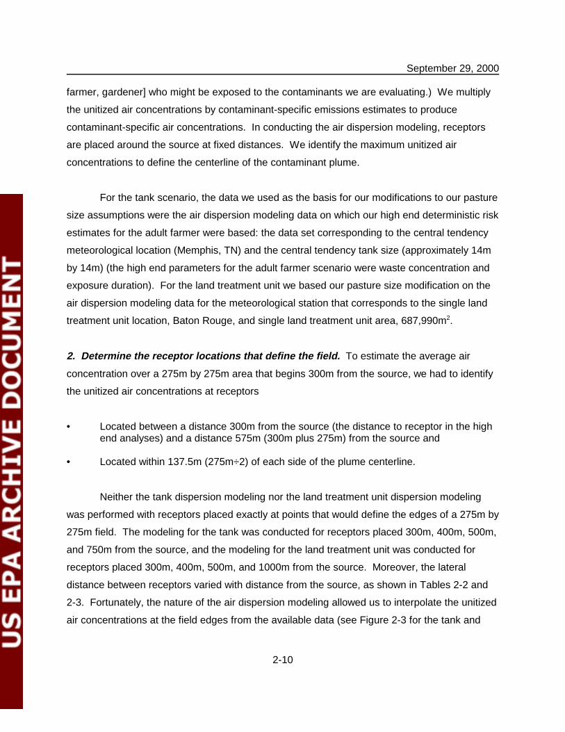
2. Determine the receptor locations that define the field. To estimate the average air

concentration over a 275m by 275m area that begins 300m from the source, we had to identify

the unitized air concentrations at receptors

• Located between a distance 300m from the source (the distance to receptor in the highend analyses) and a distance 575m (300m plus 275m) from the source and

• Located within 137.5m (275m÷2) of each side of the plume centerline.

Neither the tank dispersion modeling nor the land treatment unit dispersion modeling

was performed with receptors placed exactly at points that would define the edges of a 275m by

275m field. The modeling for the tank was conducted for receptors placed 300m, 400m, 500m,

and 750m from the source, and the modeling for the land treatment unit was conducted for

receptors placed 300m, 400m, 500m, and 1000m from the source. Moreover, the lateral

distance between receptors varied with distance from the source, as shown in Tables 2-2 and

2-3. Fortunately, the nature of the air dispersion modeling allowed us to interpolate the unitized

air concentrations at the field edges from the available data (see Figure 2-3 for the tank and

September 29, 2000

2-11

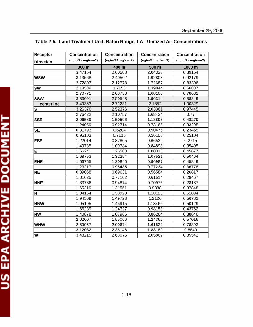
Figure 2-4 for the land treatment unit). The shaded concentrations shown in Tables 2-4 and 2-

5 present the data matrices (the air dispersion modeling output) from which the concentrations

at the lateral field edges were interpolated.

Table 2-2. Distance of Receptor Points from Source andDistance between Receptors – Tank

Distance from Source (m) Distance between Receptors (m)

300 38.7

400 50.9

500 63.7

750 94.6

Table 2-3. Distance of Receptor Points from Source andDistance between Receptors – Land Treatment Unit

Distance from Source (m) Distance between Receptors (m)

300 178.7

400 203.7

500 228.7

1000 353.7

September 29, 2000

2-12

275 m

27

5m

tank

300 m

400 m

500 m

575 m

750 m

plume centerline

* * ***

**

*

*

*

*

* interpolated point

modeled point

Figure 2-3. Air Modeling Scenario for 275 by 275 m Pasture Located 300 m from theEdge of the Wastewater Tank

September 29, 2000

2-13

275 m2

75

m

land treatment unit

300 m

400 m

500 m

575 m

1000 m

plume centerline

*

**

*

*

*

*

* interpolated point

modeled point

** * *

Figure 2-4. Air Modeling Scenario for 275 by 275 m Pasture Located 300 m from theEdge of the Land Treatment Unit

September 29, 2000

2-14

Table 2-4. Tank, Memphis, TN - Unitized Air Concentrations

Receptor

Direction

Concentration Concentration Concentration Concentration(ug/m3 / mg/s-m2) (ug/m3 / mg/s-m2) (ug/m3 / mg/s-m2) (ug/m3 / mg/s-m2)

300 m 400 m 500 m 750 mSW 1.2568 0.77034 0.52422 0.26347

1.36036 0.83322 0.56593 0.281681.5424 0.94746 0.64469 0.32066

1.84392 1.13388 0.7719 0.38329SSW 2.32404 1.44046 0.98551 0.49226

2.70777 1.68476 1.15532 0.578082.58606 1.60202 1.09507 0.543912.60314 1.61774 1.10832 0.55223

S 2.63624 1.64077 1.12551 0.561962.00194 1.23111 0.83705 0.411681.73581 1.07005 0.72866 0.359581.50264 0.92407 0.62874 0.31029

SSE 1.25577 0.77024 0.52305 0.257721.01697 0.62045 0.42023 0.206610.92195 0.56353 0.3824 0.188970.82953 0.50616 0.34313 0.16981

SE 0.72703 0.44181 0.29898 0.148470.86244 0.5265 0.35701 0.176841.02141 0.62602 0.42539 0.210771.07255 0.65529 0.44408 0.21837

ESE 1.18654 0.7293 0.49609 0.245151.32842 0.82322 0.56272 0.279871.10624 0.6794 0.46154 0.22691.2783 0.79413 0.54326 0.2697

E 1.28475 0.79691 0.5448 0.270071.23271 0.76335 0.52091 0.257541.17376 0.72208 0.49077 0.241691.52736 0.9438 0.64406 0.3198

ENE 1.86402 1.15047 0.78464 0.389871.90276 1.17311 0.79972 0.398071.66429 1.01668 0.68888 0.340221.68193 1.03258 0.70236 0.35094

NE 1.57969 0.96892 0.65975 0.332241.79242 1.09862 0.74673 0.372382.13602 1.31674 0.89816 0.448882.37193 1.46154 0.99638 0.49604

(continued)

September 29, 2000

Table 2-4. Tank, Memphis, TN - Unitized Air Concentrations

Receptor

Direction


300 m 400 m 500 m 750 m

2-15

NNE 2.62736 1.63238 1.11892 0.561272.40257 1.48303 1.01158 0.501772.46014 1.51459 1.03091 0.508423.26319 2.0155 1.37468 0.67938

N 4.70998 2.94723 2.02793 1.016465.13137 3.2088 2.20578 1.104285.06794 3.1763 2.18709 1.099574.3813 2.74817 1.89414 0.9559

NNW 3.18078 1.96877 1.34505 0.67092.85208 1.77628 1.21914 0.61462.20599 1.35984 0.9271 0.46351.94446 1.20143 0.82073 0.41383

NW 1.60932 0.9919 0.67762 0.343731.60011 0.98095 0.66656 0.332711.97633 1.22909 0.84323 0.426392.05037 1.27335 0.87209 0.43827

WNW 2.00156 1.25075 0.85977 0.433341.62487 1.00492 0.68577 0.340492.03714 1.27086 0.87229 0.436282.63879 1.64879 1.13252 0.56596

W 3.65328 2.30719 1.59568 0.80572.48129 1.53589 1.0482 0.519022.20659 1.38011 0.94865 0.475491.76247 1.09148 0.74597 0.3711

WSW 1.63511 1.00919 0.68861 0.34281.66917 1.03496 0.70879 0.356051.48373 0.9108 0.61941 0.308031.43385 0.88224 0.60111 0.30107

September 29, 2000

2-16

Table 2-5. Land Treatment Unit, Baton Rouge, LA - Unitized Air Concentrations

Receptor

Direction


300 m 400 m 500 m 1000 m3.47154 2.60508 2.04333 0.89154

WSW 3.13568 2.40502 1.92803 0.921792.72803 2.12778 1.72687 0.83396

SW 2.18539 1.7153 1.39844 0.668372.70771 2.08753 1.68106 0.78631

SSW 3.33091 2.50543 1.96314 0.88249centerline 3.49363 2.71231 2.1852 1.00329

S 3.26376 2.52376 2.03361 0.974452.76422 2.10757 1.68424 0.77

SSE 2.06589 1.50596 1.13898 0.482791.24059 0.92714 0.73165 0.33295

SE 0.81793 0.6284 0.50475 0.234650.95103 0.7116 0.56108 0.25104

ESE 1.22014 0.87805 0.66539 0.27151.49735 1.09784 0.84898 0.35495

E 1.66241 1.26503 1.00313 0.456771.68753 1.32254 1.07521 0.50464

ENE 1.56755 1.20846 0.96987 0.458491.23217 0.95485 0.77234 0.36778

NE 0.89068 0.69631 0.56584 0.268171.01625 0.77102 0.61514 0.28467

NNE 1.33786 0.94874 0.70976 0.281871.65219 1.21551 0.9388 0.37848

N 1.84154 1.38928 1.10125 0.518941.94569 1.49723 1.2126 0.56782

NNW 1.95195 1.45915 1.13466 0.501291.66239 1.24727 0.98153 0.43762

NW 1.40878 1.07966 0.86264 0.386462.02007 1.55066 1.24362 0.57016

WNW 2.59957 2.00674 1.61822 0.788923.12082 2.36146 1.88189 0.8849

W 3.48215 2.63075 2.05867 0.85542

September 29, 2000

2-17

3. Estimate air concentrations at receptors located 575m from the source. Because the

ISC model simulates a gaussian plume in any given direction, we could estimate air

concentrations at 575 m from the source (i.e., the furthest edge of the 275m by 275m field) by

plotting the concentration data for the 300m, 400m, 500m, and 750m(tank) or 1000m(land

treatment unit) distances on a log-log graph. These graphs are shown in Figure 2-5 for the

tank and 2-6 for the land treatment unit. For a given increment of distance off the plume

centerline, each line on the graph represents the change in concentration with distance from

the source. We used these graphs to predict the concentrations at 575m by drawing a vertical

line at 575m that intersects with each of the plotted lines, then reading from the graph the

concentrations at various increments of distance off the plume centerline, 575m from the

source.

4. Estimate air concentrations at receptors located 137.5m off of the plume centerline.

The concentration profiles for receptor points at a given distance (for example, 300m from the

source) could be used to interpolate the concentration at a distance 137.5m off of the centerline

of the plume in either direction, that is, the concentrations at the lateral edges of the pasture.

Each of the profiles shown in Figures 2-7 and 2-8 represents the change in concentration

moving away from the plume centerline at a given distance from the source. As shown in the

figure, we can derive the concentration at 137.5m on either side of the plume centerline by

drawing a line at 137.5m. The resulting concentration estimates at 300, 400, 500, and 575 m

from the source were read directly from the graph.

September 29, 2000

2-18

Figure 2-5. Estimating Concentrations at 575 m - Tank

0.1

1

10

100 1000

Distance From Source (m )

Con

cent

ratio

n

centerline -3

centerline -2

centerline -1

centerline

centerline +1

centerline +2

centerline +3

Figure 2-6. Estimating Concentrations at 575m - Land Treatment Unit

0.1

1

10

100 1000Distance from Source (m)

Con

cent

ratio

n

centerline -3

centerline -2

centerline -1

centerline

centerline +1

centerline +2

centerline +3

September 29, 2000

2-19

Figure 2-7. Estimating Concentrations at 137.5 m - Tank

0

1

2

3

4

5

6

-250 -225 -200 -175 -150 -125 -100 -75 -50 -25 0 25 50 75 100 125 150 175 200 225 250

Distance from Plume Centerline (m)

Con

cent

ratio

n 300 m

400 m

500 m

575 m

Figure 2-8. Estimating Concentrations at 137.5m - Land Treatment Unit

0

1

2

3

4

-900 -800 -700 -600 -500 -400 -300 -200 -100 0 100 200 300 400 500 600 700 800 900

Distance from Plume Centerline (m)

Con

cent

ratio

n 300 m

400 m

500 m

575 m

September 29, 2000

2-20

5. Calculate the average air concentration over a 275m by 275m pasture. Using the air

concentrations derived in Steps 3 and 4 above, we created a matrix of air concentration points

that represent the pasture, and performed the simple calculations needed to produce an area

average. Figures 2-9 and 2-10 present the concentrations for the 275m by 275m pasture

located 300m from a wastewater tank and the land treatment unit, respectively (for

convenience, values were rounded at two decimal places). Tables 2-6 and 2-7 show the

calculations. For each distance from the source (that is, 300, 400, 500, and 575m), only those

air concentrations that fall within the 275m width were used to calculate the distance-specific

average. For example, for the tank, we used nine receptor locations to estimate the average

concentration at 300m from the source. The concentrations corresponding to adjacent points

were averaged, and then the resulting concentrations were weighted according to the increment

of distance they represent, to calculate an average concentration at 300 meters, as follows:

[( . . . . . . ) . ] [( . . ) . ]4 921 3986 2 862 510 4 725 3781 38 7 2 430 3065 214

275

+ + + + + + +x x

To avoid biasing the data by the number of receptor locations, we calculated the average

concentration at each distance from the source prior to generating a pasture area average. For

example, for the tank, the concentrations corresponding to adjacent distances from the source

were averaged, and the resulting concentrations were weighted according to the increment of

distance they represent, to calculate a pasture area average concentration, as follows:

[( . . ) ] ( . )3363 2 355 100 179 75

275

+ +x x

For the tank, dividing the maximum concentration at 300m (5.13 ug/m3 / mg/s-m2, the

concentration we used in the 1999 risk analysis) into the pasture area average of 2.568 ug/m3 /

mg/s-m2 results in a ratio of 0.50 or a 50% reduction in the air concentration, therefore in risk.

September 29, 2000

2-21

tank

300 m

plume centerline

1.1 1.6 1.75 1.72 1.55

1.37 2.03 2.21 2.19 1.89 1.8

400 m

500 m

575 m

1.65 2.02 2.95 3.21 3.18 2.75

2.4 2.46 3.26 4.71 5.13 5.07 4.38 3.18 2.95

1.3

interpolated concentrationsshown in bold font

2.2

Figure 2-9. Air Concentrations for 275 by 275 m Pasture Located 300 m fromWastewater Tank (concentrations in ug/m3 / mg/s-m2)

September 29, 2000

2-22

land treatment unit

300 m

plume centerline

1.8 1.9 1.88

2.19 2.1

400 m

500 m

575 m

2.6 2.71

3.41 3.49 3.32

2.08

interpolated concentrationsshown in bold font

2.61

Figure 2-10. Air Concentrations for 275 by 275 m Pasture Located 300 m fromLand Treatment Unit (concentrations in ug/m3 / mg/s-m2)

September 29, 2000

2-23

Table 2-6. Calculation of Average Concentration Over 275m by 275m Pasture – Tank

300 m 400 m 500 m 575 mDistance from

PlumeCenterline

Concentrationug/m3/mg/s-m2

AverageConcentration

BetweenAdjacent Points

Distancefrom

PlumeCenterline



BetweenAdjacent

Points

Distance fromPlume

Centerline



BetweenAdjacent

Points

Distance fromPlume

Centerline



BetweenAdjacent

Points

-154.8 2.40257

-137.5 2.4 -152.7 1.51459 -191.1 1.03091 -219 0.82.43007

-116.1 2.46014 -137.5 1.65 -137.5 1.3 -146 1.082.86167 1.83275 1.33734

-77.4 3.26319 -101.8 2.0155 -127.4 1.37468 -137.5 1.13.98659 2.48137 1.70131 1.35000

-38.7 4.70998 -50.9 2.94723 -63.7 2.02793 -73 1.64.92068 3.07802 2.11686 1.67500

0 5.13137 0 3.2088 0 2.20578 0 1.755.09966 3.19255 2.19644 1.73500

38.7 5.06794 50.9 3.1763 63.7 2.18709 73 1.724.72462 2.96224 2.04062 1.63500

77.4 4.3813 101.8 2.74817 127.4 1.89414 137.5 1.553.78104 2.47409 1.84707

116.1 3.18078 137.5 2.2 137.5 1.8 146 1.53.06539

137.5 2.95 152.7 1.96877 191.1 1.34505 219 1.05

154.8 2.85208

distance-weightedaverage concentration

3.998 2.727 1.983 1.605

distance-weighted pasture average 2.568300m maximum ÷ pasture average: 0.50

September 29, 2000

2-24

Table 2-7. Calculation of Average Concentration Over 275m by 275m Pasture – Land Treatment Unit

300 m 400 m 500 m 575 mDistance from

PlumeCenterline



BetweenAdjacent Points

Distancefrom

PlumeCenterline



BetweenAdjacent

Points

Distance fromPlume

Centerline



BetweenAdjacent

Points

Distance fromPlume

Centerline



BetweenAdjacent

Points

-178.7 3.33091 -203.7 2.50543 -228.7 1.96314 -248 1.7

-137.5 3.41 -137.5 2.6 -137.5 2.08 -137.5 1.83.4518 2.6562 2.1326 1.8500

0 3.49363 0 2.71231 0 2.1852 0 1.93.4068 2.6612 2.1426 1.8900

137.5 3.32 137.5 2.61 137.5 2.1 137.5 1.88

178.7 3.26376 203.7 2.52376 228.7 2.03361 248 1.8

distance-weightedaverage concentration

3.429 2.659 2.138 1.87

distance-weighted pasture average: 2.525300m maximum ÷ pasture average: 0.72

September 29, 2000

2-25

For the land treatment unit, dividing the maximum concentration at 300m (3.49 ug/m3 / mg/s-

m2, the concentration we used in the 1999 risk analysis) into the pasture area average of 2.525

ug/m3 / mg/s-m2 results in a ratio of 0.72 or a 28% reduction in the air concentration, therefore

in the portion of the risk estimate attributable to the air pathway (part of the nongroundwater

pathway risk associated with the land treatment unit is due to the erosion/runoff pathway).

Section 5.3 summarizes how assuming a larger pasture size would influence our high

end deterministic risk estimates for the aerated biological treatment tank and land treatment

unit waste management scenarios.

2.3 Evaluation of the Exposure Scenario as it Relates to the Probabilistic Analyses

We stated on page 2-38 of the 1999 Risk Assessment TBD that in our probabilistic

analyses we assumed that individuals (receptors) live between 50 and 1000 meters from the

waste management unit, and randomly evaluated receptors located 50, 75, 100, 200, 300, 500,

or 1000m from the waste management unit. In evaluating commenters’ concerns regarding

the overly conservative nature of our exposure assumptions, we acknowledged that the

distances we chose to represent the location of receptors relative to the waste management

units were too heavily weighted toward locations close to the waste management units. That is,

the distances between 50m and 100m are 25 meters apart; the distances between 100m and

300m are 100 meters apart; the distance between 300m and 500m is 200 meters apart; and the

distance between 500m and 1000m is 500 meters apart. As a result, our probabilistic risk

percentiles likely are somewhat lower than they would have been if the distances we evaluated

had been spaced equally. We expect this effect to be more pronounced for the wastewater

tank scenario, since the air concentrations associated with the plume from the tank vary more

greatly with distance than those for the land treatment unit. This is because the tank source is

so much smaller than the land treatment unit source. Any overestimate of our probabilistic risk

results is not particularly consequential since our listing decisions were based primarily on the

results of the deterministic analyses, which, as discussed in this Addendum, we reevaluated in

response to commenters’ concerns.

September 29, 2000

3-1

3. ESTIMATING EXPOSURE POINT CONCENTRATIONS

This section provides technical information that supplements that provided in Section 3

of the 1999 Risk Assessment Technical Background Document. Section 3 of the background

document described how EPA used models to estimate contaminant concentrations at a

receptor’s point of exposure.


• A discussion of how the removal of solids from wastewater prior to aerated biologicaltreatment would influence the risk estimates for chlorinated aliphatics wastewaters; and

• A mass balance correction for the land treatment unit erosion pathway analysis.

3.1 Removal of Solids from Wastewater Prior to Aerated Biological Treatment

To evaluate the risks from management of wastewaters, EPA modeled the contaminant

emissions from aerated biological wastewater treatment tanks. In the proposed rule EPA

explained that significant risk was associated with exposure to dioxins emitted from aerated

biological treatment tanks. Commenters on the proposed rule asserted that EPA failed to

account for the fact that almost all of the dioxins in wastewaters are sorbed to solids and are

removed in primary clarifiers prior to aeration. EPA agrees with the commenters concerns that

we failed to accurately account for the fact that in aerated biological wastewater treatment

systems, at least some solids removal generally will occur between the headworks of the

wastewater treatment system and the influent to an aerated biological treatment tank. In the

preamble to the proposed rule, EPA specifically stated that we selected wastewater data for

evaluation that we believed represented the concentrations of contaminants in wastewaters at

the influent (headworks) of treatment systems that are used to manage only wastewaters from

the production of chlorinated aliphatic chemicals (“dedicated” chlorinated aliphatics wastewater

samples; 64 FR 46483). In retrospect, our assumption that the same data that represent

contaminant concentrations at the headworks of wastewater treatment systems could represent

September 29, 2000

2See the Listing Background Document for the Chlorinated Aliphatics ListingDetermination (Final Rule), June 30, 2000, for a description of this information.

3-2

contaminant concentrations at the influent to aerated biological wastewater treatment tanks was

somewhat flawed.

We reviewed information previously provided to us in industry survey responses and

determined that of the eleven facilities that employ aerated biological processes to treat their

wastewaters, nine employ primary clarification or other processes that have the effect of

removing solids from wastewaters prior to their discharge to aerated biological treatment tanks.

(One of these nine facilities is the facility from which we collected the “high end” wastewater

sample used in the risk analysis that served as the basis for our proposed listing decision.) The

remaining two facilities perform wastewater equalization in tanks prior to aerated biological

treatment. One of these two facilities also employs wastewater pH adjustment with resultant

precipitation of metal hydroxides prior to aerated biological treatment2. Both of these processes

are expected to result in at least some solids removal from the wastestream. Moreover, EPA

does not anticipate that treatment of the wastewaters in units such as primary clarifiers and

equalization basins would result in dioxin air emissions greater than those that we originally

predicted from aerated biological treatment tanks, because primary clarifiers are, by design,

quiescent units (Metcalf and Eddy, 1991, p. 472), and we have no information that leads us to

believe that the equalization tanks in use by the facilities are agitated.

To model the aerated biological treatment tanks correctly, that is, to determine what the

appropriate influent concentration to the biological treatment tank should be, would have

required that EPA model the wastewater treatment train from the point where wastewater

enters the headworks of the treatment system to the point where the wastewater enters the

aerated biological tank. Metcalf and Eddy (1991, p. 473) state that “efficiently designed and

operated primary sedimentation tanks should remove from 50 to 70 percent of the suspended

solids...” from wastewater. Consequently, we estimated how our emissions estimates would

differ if we assumed alternately that 50 percent and 70 percent of the solids in chlorinated

aliphatics wastewater analysis we used in our high end analysis were removed prior to

discharge to the aerated biological treatment tank. Specifically, we assumed that the dioxins in

September 29, 2000

3 In public comments, industry commenters conservatively assumed that the wastewatersolids are only 3% organic carbon.

3-3

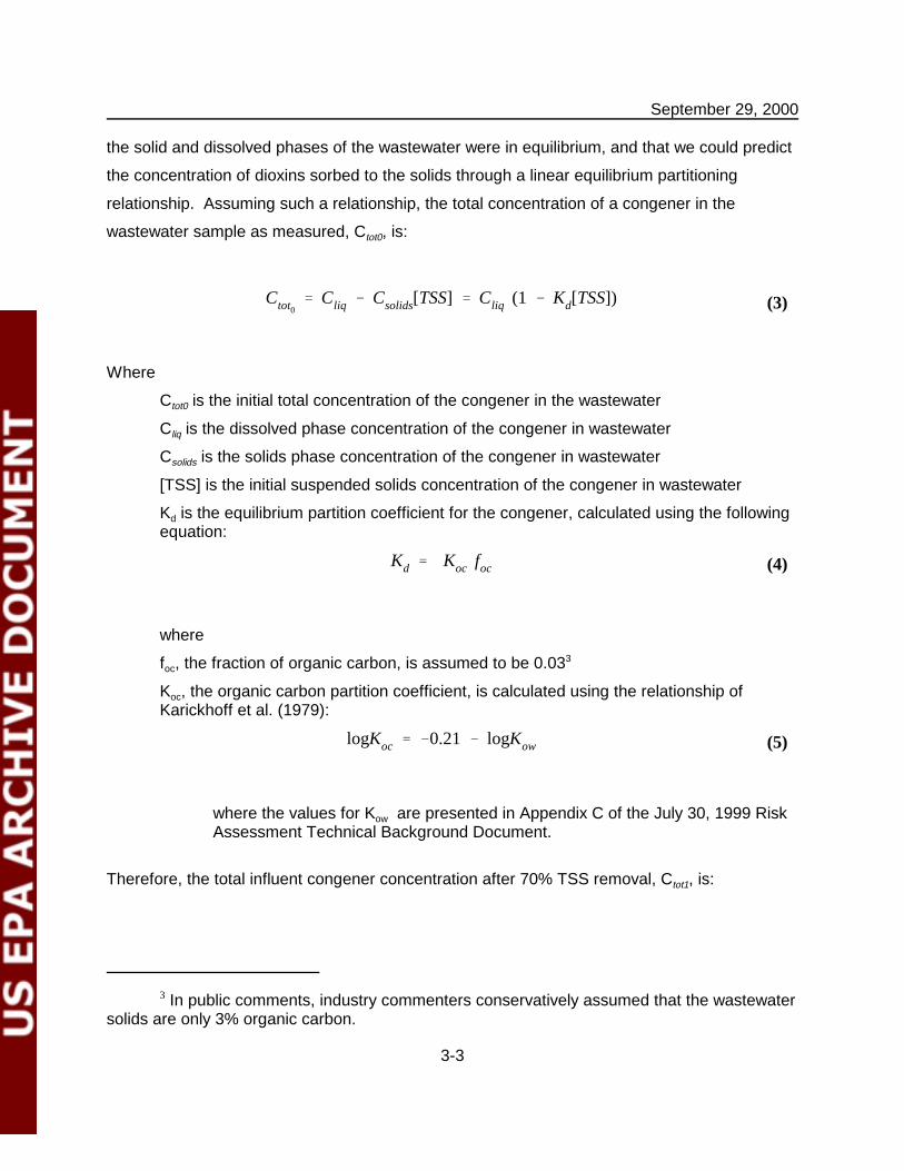
Ctot0ÿ Cliq � Csolids[TSS] ÿ Cliq (1 � Kd[TSS]) (3)

Kd ÿ Koc foc (4)

logKoc ÿ �0.21 � logKow (5)

the solid and dissolved phases of the wastewater were in equilibrium, and that we could predict

the concentration of dioxins sorbed to the solids through a linear equilibrium partitioning

relationship. Assuming such a relationship, the total concentration of a congener in the

wastewater sample as measured, Ctot0, is:

Where

Ctot0 is the initial total concentration of the congener in the wastewater

Cliq is the dissolved phase concentration of the congener in wastewater

Csolids is the solids phase concentration of the congener in wastewater

[TSS] is the initial suspended solids concentration of the congener in wastewater

Kd is the equilibrium partition coefficient for the congener, calculated using the followingequation:

where

foc, the fraction of organic carbon, is assumed to be 0.033

Koc, the organic carbon partition coefficient, is calculated using the relationship ofKarickhoff et al. (1979):

where the values for Kow are presented in Appendix C of the July 30, 1999 RiskAssessment Technical Background Document.

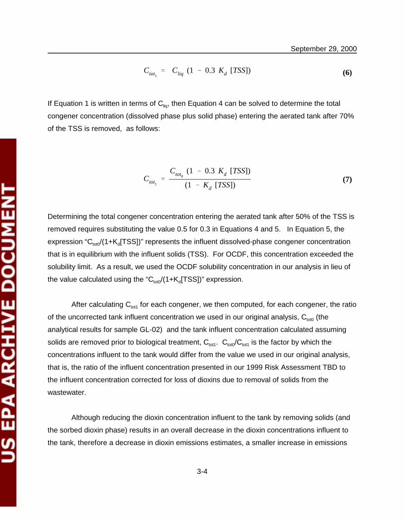
Therefore, the total influent congener concentration after 70% TSS removal, Ctot1, is:

September 29, 2000

3-4

Ctot1ÿ Cliq (1 � 0.3 Kd [TSS]) (6)

Ctot1ÿ

Ctot0(1 � 0.3 Kd [TSS])

(1 � Kd [TSS])(7)

If Equation 1 is written in terms of Cliq, then Equation 4 can be solved to determine the total

congener concentration (dissolved phase plus solid phase) entering the aerated tank after 70%

of the TSS is removed, as follows:

Determining the total congener concentration entering the aerated tank after 50% of the TSS is

removed requires substituting the value 0.5 for 0.3 in Equations 4 and 5. In Equation 5, the

expression “Ctot0/(1+Kd[TSS])” represents the influent dissolved-phase congener concentration

that is in equilibrium with the influent solids (TSS). For OCDF, this concentration exceeded the

solubility limit. As a result, we used the OCDF solubility concentration in our analysis in lieu of

the value calculated using the “Ctot0/(1+Kd[TSS])” expression.

After calculating Ctot1 for each congener, we then computed, for each congener, the ratio

of the uncorrected tank influent concentration we used in our original analysis, Ctot0 (the

analytical results for sample GL-02) and the tank influent concentration calculated assuming

solids are removed prior to biological treatment, Ctot1. Ctot0/Ctot1 is the factor by which the

concentrations influent to the tank would differ from the value we used in our original analysis,

that is, the ratio of the influent concentration presented in our 1999 Risk Assessment TBD to

the influent concentration corrected for loss of dioxins due to removal of solids from the

wastewater.

Although reducing the dioxin concentration influent to the tank by removing solids (and

the sorbed dioxin phase) results in an overall decrease in the dioxin concentrations influent to

the tank, therefore a decrease in dioxin emissions estimates, a smaller increase in emissions

September 29, 2000

3-5

also occurs due to reducing the TSS concentration in the tank, as shown in Table D.3-3 of

Appendix D.3 in the 1999 Risk Assessment Technical Background Document. This increase in

emissions occurs because reducing the TSS influent to the tank reduces the mass of solids in

the tank onto which dioxins can sorb. Therefore, the last step of the evaluation is to correct the

emissions estimate to account for this emissions increase. We approximated this increase in

emissions from the results of the sensitivity analyses for dioxins that we generated in

developing Table D.3-3 of the 1999 Risk Assessment TBD. These sensitivity results are

presented below in Table 3-1. Specifically, we assumed that removing 50 percent of the TSS

results in increasing emissions by a factor of 1.25 and removing 70 percent of the TSS results

in increasing emissions by a factor of 1.47. In the CHEMDAT8 model the relationship between

TSS and emissions also is dependent on the solids balance with TOC. Consequently, the

results of any sensitivity analysis will depend greatly on the characteristics of a given waste

stream.

To account for both the decrease in emissions due to the reduced concentrations of

dioxins entering the tank and the smaller increase in emissions due to the reduced solids

concentration in the tank, we divided the value for Ctot0/Ctot1 calculated above by 1.25 (for 50

percent solids removal) or 1.47 (for 70 percent solids removal) to obtain the values in Tables 3-

2 and 3-3. The values presented in Tables 3-2 and 3-3 are our estimates of the factors by

which our emissions estimates presented in the 1999 Risk Assessment TBD exceed the

emissions predicted given the assumption that 70 percent and 50 percent of the solids,

respectively, are removed from the wastewater prior to aerated biological treatment. Dividing

our 1999 congener-specific risk estimates by the factors presented in Tables 3-2 and 3-3

produces revised risk estimates that account for solids removal prior to aerated biological

treatment.

3-6

Table 3-1. Sensitivity Results for the Wastewater Tank Analysis

ContaminantsBaseline Emissions

Baton Rouge MetStation,

Central Tendency Tank,Average Concentration

Emissions whenTSS (or Biomass Solids) in Influent Are:

Increased by a factor of 2 Decreased by a factor of 2

(Mg/yr) (Mg/yr) % difference (Mg/yr) % differenceAcetone 6.74E-04 6.74E-04 0.0 6.74E-04 0.0Allyl Chloride 1.35E-03 1.35E-03 0.0 1.35E-03 0.0Aminobiphenyl,4- 3.68E-07 3.67E-07 -0.1 3.68E-07 0.1Benzoic Acid 2.24E-05 2.24E-05 -0.1 2.24E-05 0.0Benzyl Alcohol 7.09E-07 7.08E-07 -0.1 7.09E-07 0.0Bis(2-chloroethyl)ether 6.18E-04 6.18E-04 -0.1 6.19E-04 0.0Bis(2-chloroisopropyl)ether 3.20E-04 3.20E-04 -0.1 3.20E-04 0.0Bis(2-ethylhexyl)phthalate 5.15E-08 3.51E-08 -31.9 6.73E-08 30.6Bromodichloromethane 4.24E-04 4.24E-04 0.0 4.24E-04 0.0Bromoform 1.47E-04 1.47E-04 -0.1 1.47E-04 0.0Carbon Disulfide 9.35E-04 9.35E-04 0.0 9.35E-04 0.0Chlorobenzene 2.14E-04 2.14E-04 0.0 2.14E-04 0.0Chloro-1,3,-butadiene,2- 1.97E-03 1.97E-03 0.0 1.97E-03 0.0Chloroethane (Ethyl Chloride) 1.79E-03 1.79E-03 0.0 1.79E-03 0.0Chloroform 4.28E-02 4.28E-02 0.0 4.28E-02 0.0Cresol(-o) 1.49E-07 1.49E-07 0.0 1.49E-07 0.0Cresol(-p) 1.14E-07 1.14E-07 0.0 1.14E-07 0.0Dibromochloromethane 6.57E-04 6.56E-04 -0.2 6.58E-04 0.1Dichloroethane(1,2) 3.98E-03 3.98E-03 0.0 3.98E-03 0.0Dichloroethene 1,2 Trans 6.63E-04 6.62E-04 0.0 6.63E-04 0.0Dichloroethylene, 1,2 - Cis 8.10E-04 8.10E-04 0.0 8.10E-04 0.0Diethyl Phthalate 2.10E-06 2.10E-06 -0.1 2.10E-06 0.0Dimethyl Phthalate 1.90E-08 1.90E-08 0.0 1.90E-08 0.0Di-n-octyl Phthalate 4.87E-06 3.20E-06 -34.3 6.58E-06 35.2Ethylbenzene 3.64E-04 3.64E-04 -0.1 3.64E-04 0.0Hexachlorobenzene 1.17E-03 1.03E-03 -11.4 1.25E-03 6.9HpCDD, 1,2,3,4,6,7,8- 2.31E-10 1.46E-10 -36.6 3.24E-10 40.7HpCDF, 1,2,3,4,6,7,8- 3.93E-08 2.50E-08 -36.4 5.48E-08 39.4HpCDF, 1,2,3,4,7,8,9- 8.45E-09 5.39E-09 -36.2 1.18E-08 39.7HxCDD, 1,2,3,4,7,8- 5.33E-11 3.39E-11 -36.4 7.47E-11 40.2HxCDD, 1,2,3,6,7,8- 1.35E-10 8.62E-11 -36.0 1.87E-10 39.1HxCDD, 1,2,3,7,8,9- 1.38E-10 8.81E-11 -36.0 1.91E-10 39.1HxCDF, 1,2,3,4,7,8- 7.15E-09 4.58E-09 -35.9 9.94E-09 39.0HxCDF, 1,2,3,6,7,8- 1.65E-09 1.06E-09 -36.1 2.30E-09 39.3HxCDF, 1,2,3,7,8,9- 9.06E-10 5.80E-10 -36.0 1.26E-09 39.2HxCDF, 2,3,4,6,7,8- 1.54E-09 9.87E-10 -36.0 2.15E-09 39.2Mercury 1.14E-04 1.13E-04 -1.2 1.15E-04 1.0Methyl Ethyl Ketone, 2-Butanone 6.25E-04 6.24E-04 -0.2 6.25E-04 0.1Methylene Chloride, Dichloromethane 1.26E-03 1.26E-03 0.0 1.26E-03 0.0OCDD, 1,2,3,4,5,7,8,9- 5.18E-12 3.29E-12 -36.4 7.26E-12 40.2OCDF, 1,2,3,4,6,7,8,9- 1.11E-09 7.02E-10 -36.8 1.57E-09 41.0PeCDF, 2,3,4,7,8- 6.55E-10 4.23E-10 -35.4 9.03E-10 37.8Pentachlorophenol 4.39E-08 4.36E-08 -0.8 4.41E-08 0.4Phenol 4.98E-07 4.98E-07 0.0 4.98E-07 0.0Styrene 1.14E-03 1.14E-03 -0.1 1.14E-03 0.1TCDD, 2,3,7,8- 2.48E-11 1.62E-11 -34.6 3.37E-11 36.0TCDF, 2,3,7,8- 1.48E-10 9.75E-11 -34.2 2.00E-10 35.1Tetrachloroethene 8.29E-04 8.29E-04 0.0 8.29E-04 0.0Trichloroethylene 8.36E-06 8.36E-06 0.0 8.36E-06 0.0Trichlorophenol 2,4,5 1.63E-06 1.63E-06 -0.1 1.63E-06 0.1Trichlorophenol 2,4,6 1.46E-04 1.44E-04 -1.3 1.47E-04 0.7

Average impact as compared to Baseline emissions 12% decrease 13% increase

September 29, 2000

3-7

Table 3-2.Ratio of the 1999 High End Emissions Estimate and

Emissions Estimate that Assumes Solids (TSS)Removal Prior to Aerated Biological Treatment

70% TSS Removal Efficiency1,2,3,4,6,7,8-HpCDD 2.26

1,2,3,4,6,7,8-HpCDF 0.07

1,2,3,4,7,8,9-HpCDF 0.26

1,2,3,4,7,8-HxCDD 2.25

1,2,3,6,7,8-HxCDD 2.22

1,2,3,7,8,9-HxCDD 2.25

1,2,3,4,7,8-HxCDF 2.22

1,2,3,6,7,8-HxCDF 2.22

1,2,3,7,8,9-HxCDF 0

2,3,4,6,7,8-HxCDF 2.22

2,3,4,7,8-PeCDF 2.16

2,3,7,8-TCDD 2.08

2,3,7,8-TCDF 2.03

OCDD 0.024

OCDF 0.00063

Table 3-3.Ratio of the 1999 High End Emissions Estimate and

Emissions Estimate that Assumes Solids (TSS)Removal Prior to Aerated Biological Treatment

50% TSS Removal Efficiency1,2,3,4,6,7,8-HpCDD 1.60

1,2,3,4,6,7,8-HpCDF 0.05

1,2,3,4,7,8,9-HpCDF 0.19

1,2,3,4,7,8-HxCDD 1.60

1,2,3,6,7,8-HxCDD 1.59

1,2,3,7,8,9-HxCDD 1.60

1,2,3,4,7,8-HxCDF 1.59

1,2,3,6,7,8-HxCDF 1.59

1,2,3,7,8,9-HxCDF 0

2,3,4,6,7,8-HxCDF 1.59

2,3,4,7,8-PeCDF 1.57

2,3,7,8-TCDD 1.54

2,3,7,8-TCDF 1.53

OCDD 0.017

OCDF 0.00045

September 29, 2000

3-8

Based on our calculations, removing solids from chlorinated aliphatics wastewaters prior

to biological treatment might reduce the high end deterministic risk estimate by a factor of

ranging from approximately 0.67 (for 70 percent removal of solids) to 0.94 (for 50 percent

removal of solids). As explained on p. 3-2 of the 1999 Risk Assessment Technical Background

Document, we originally constrained (“capped”) the influent concentrations of congeners in the

wastewaters at their aqueous solubility concentrations to account for the fact that dioxins are

strongly hydrophobic and are expected to be sorbed to solids preferentially in the wastewater

influent, thus are unlikely to exist in the dissolved phase in excess of their solubility limits (see

also the Errata for Section 3 in this Addendum). Because the wastewaters contained both

dissolved- and particle-phase dioxins (the samples were not filtered prior to analysis), we

corrected our application of this constraint by applying it directly to the dissolved-phase

congener concentrations (that is, the expression “Ctot0/(1+Kd[TSS])” from Equation 7).

Consequently, the ratios presented in Tables 3-2 and 3-3 are less than 1 for 1,2,3,4,6,7,8-

HpCDF, 1,2,3,4,7,8,9-HpCDF, OCDD, and OCDF. That is, in our revised analysis, the

concentrations of these congeners in the wastewater exceeded their solubility limits. Therefore,

the concentrations of these four congeners in the influent wastewater were greater in our

reevaluation than they were in the 1999 analysis, although the concentrations of all of the other

congeners decreased.

Section 5.3 summarizes how accounting for solids removal prior to aerated biological

treatment of wastewaters would influence our high end deterministic risk estimates for

chlorinated aliphatics wastewaters.

3.2 Mass Balance Correction for the Land Treatment Unit Erosion Pathway Analysis

To predict the contaminant concentration in a receiving field located near the land

treatment unit, we developed a conceptual model for overland transport based on the

assumption that the system (i.e., the land treatment unit, the field, and the buffer areas that

comprise the drainage subbasin) is at steady state. The steady-state assumption was crucial to

developing a modeling approach that could be implemented within a concatenation of

spreadsheet models that are designed to model steady state processes. The overland

transport model relies on the Universal Soil Loss Equation (USLE) to predict soil loads to the

September 29, 2000

3-9

waterbody and receiving field; application of the USLE in this context implies a steady state

system. Moreover, the use of a sediment delivery ratio to predict the fraction of eroded soil that

is deposited in the area between the land treatment unit and the waterbody implicitly assumes

that the sediment delivery does not change with time.

The overland transport model used the maximum 9-year average soil concentration

predicted by the source partitioning model as the contaminant concentration in the land

treatment unit. Because the system was assumed to be at steady state, we fixed the land

treatment unit concentration during the period of the simulation, effectively creating an infinite

source (defined as a source with a fixed concentration that does not deplete over time).

However, the drainage subbasin is not really a steady state system. In reality, the land

treatment unit concentration would decrease with time until the land treatment unit was "clean",

and some or all of the contaminant on the receiving field would be transported to the stream via

soil erosion and runoff mechanisms. This type of contaminant profile would not resemble

steady state, but rather, a transient system with a concentration profile for the field that

increases with time, reaches a peak, and then decreases with time. In other project analyses

assuming an infinite source, we found that it takes roughly 50 years for the model to reach

steady state but, as our calculations have demonstrated, the contaminant mass is exhausted

well before that time for the land treatment unit. In essence our calculations show that the total

land treatment unit emissions from soil erosion over an 80 year time period are roughly a factor

of 9 above the emissions possible given the mass loaded over the active life of the unit. Table

3-4 provides this calculation. (Both the central tendency and high end emissions estimates for

the land treatment unit are provided in detail in Tables 3-5 and 3-6.) This result is not

unexpected because the source is not allowed to deplete over the simulation period so that

steady state conditions may be approximated. Section 5.3 summarizes how including this

factor in our exposure analyses would influence our high end deterministic estimate of risk.

The Agency recognizes this as a limitation of the overland transport model and has

since developed a more rigorous modeling approach that simulates the changes and source

and field concentration with time (that is, the model develops concentration profiles). However,

September 29, 2000

3-10

Table 3-4. Erosion Mass Balance Calculation – Land Treatment Unit (LTU)

Total High End Dioxin Load to LTU Available to be Emitted (g TCDD TEQ), based on 907 ng/kgwaste concentration and 624 Mton/year waste generation rate:

Annual Over 40-year Active Life

0.57 23

High End Emissions (g TCDD TEQ) (from Table 3-6):

AnnualOver 80-year Active and

Inactive Life

Vapor 0.107 8.56

Particulate (PM10) 0.0091 0.72

Particulate (PM30) 0.014 1.1

Erosion 1.4 109.6

Runoff 0.00027 0.022

Leaching 0.00005 0.004

Total 1.5 120.0

Mass TCDD (g TCDD TEQ) Actually Available for Erosion =Total Load to LTU - Vapor and Particulate Emissions - Runoff Emissions - LeachingEmissions:

AnnualOver 80-year Active and

Inactive Life

0.436 12.244

Factor by which erosion may be overestimated(TEQ erosion emissions/TEQ Available for Erosion): 9

3-11

Table 3-5. Central Tendency TCDD TEQ Emission Estimates for the EDC/VCM Land Treatment Unit

Congener TEF Vaporemissions(g/m2-yr)

Vaporemissions

(g/yr)

Particulateemissions(PM 10)

(g/m2-yr)


(g/yr)


(g/m2-yr)


(g/yr)

Erosionemissions(g/m2-yr)

Erosionemissions

(g/yr)

Runoffemissions(g/m2-yr)

Runoffemissions

(g/yr)

LeachingEmission

(g/yr)

Totalemissions

(g/yr)

2,3,7,8-TCDD 1 NA NA NA NA NA NA NA NA NA NA NA NA

1,2,3,4,5,7,8,9-OCDD 0.001 2.4E-11 1.7E-05 3.7E-11 2.6E-05 5.6E-11 3.8E-05 5.6E-09 3.9E-03 7.7E-13 5.3E-07 9.5E-8 3.9E-03

1,2,3,7,8,9-HxCDD 0.1 1.3E-10 8.9E-05 7.9E-12 5.5E-06 1.2E-11 8.2E-06 1.2E-09 8.2E-04 3.3E-13 2.3E-07 4.2E-8 9.3E-04

1,2,3,4,6,7,8-HpCDD 0.01 1.7E-10 1.2E-04 3.8E-11 2.6E-05 5.6E-11 3.9E-05 5.7E-09 3.9E-03 1.9E-13 1.3E-07 2.4E-8 4.1E-03

OCDF 0.001 2.1E-10 1.4E-04 1.8E-10 1.2E-04 2.7E-10 1.9E-04 2.7E-08 1.9E-02 2.3E-13 1.6E-07 2.8E-8 1.9E-02


1,2,3,7,8-PeCDD 0.5 NA NA NA NA NA NA NA NA NA NA NA NA

2,3,7,8-TCDF 0.1 4.6E-11 3.1E-05 1.3E-12 8.9E-07 1.9E-12 1.3E-06 2.0E-10 1.3E-04 3.1E-13 2.1E-07 4.0E-8 1.7E-04

1,2,3,4,7,8,9-HpCDF 0.01 9.8E-10 6.7E-04 5.8E-11 4.0E-05 8.7E-11 6.0E-05 8.8E-09 6.1E-03 5.9E-13 4.1E-07 7.5E-8 6.8E-03

2,3,4,7,8-PeCDF 0.5 1.4E-09 9.6E-04 7.5E-11 5.1E-05 1.1E-10 7.7E-05 1.1E-08 7.8E-03 7.3E-12 5.0E-06 9.3E-7 8.9E-03


1,2,3,6,7,8-HxCDF 0.1 1.5E-09 1.0E-03 1.2E-10 8.6E-05 1.9E-10 1.3E-04 1.9E-08 1.3E-02 5.2E-12 3.6E-06 6.5E-7 1.4E-02






Total TEQ 1.5E-08 1.0E-02 1.2E-09 7.9E-04 1.7E-09 1.2E-03 1.7E-07 1.2E-01 3.2E-11 2.2E-05 4.1E-6 1.3E-01

3-12

Table 3-6. High End TCDD TEQ Emission Estimates for the EDC/VCM Land Treatment Unit

Congener TEF Vaporemissions(g/m2-yr)

Vaporemissions

(g/yr)


(g/m2-yr)


(g/yr)


(g/m2-yr)


(g/yr)

Erosionemissions(g/m2-yr)

Erosionemissions

(g/yr)

Runoffemissions(g/m2-yr)

Runoffemissions

(g/yr)

LeachingEmission

(g/yr)

Totalemissions

(g/yr)

2,3,7,8-TCDD 1 1.4E-08 9.8E-03 4.3E-10 3.0E-04 6.4E-10 4.4E-04 6.5E-08 4.5E-02 7.9E-11 5.5E-05 9.6E-6 5.5E-02

1,2,3,4,5,7,8,9-OCDD 0.001 6.7E-11 4.6E-05 1.1E-10 7.4E-05 1.6E-10 1.1E-04 1.6E-08 1.1E-02 2.3E-12 1.5E-06 2.5E-7 1.1E-02


1,2,3,4,6,7,8-HpCDD 0.01 5.3E-10 3.7E-04 1.2E-10 8.6E-05 1.9E-10 1.3E-04 1.9E-08 1.3E-02 6.4E-13 4.4E-07 7.2E-8 1.4E-02

OCDF 0.001 3.9E-09 2.7E-03 3.5E-09 2.4E-03 5.3E-09 3.6E-03 5.3E-07 3.7E-01 4.5E-12 3.1E-06 5.1E-7 3.8E-01

1,2,3,4,7,8-HxCDD 0.1 NA NA NA NA NA NA NA NA NA NA NA NA

1,2,3,7,8-PeCDD 0.5 NA NA NA NA NA NA NA NA NA NA NA NA

2,3,7,8-TCDF 0.1 4.6E-09 3.2E-03 1.7E-10 1.2E-04 2.6E-10 1.8E-04 2.6E-08 1.8E-02 4.0E-11 2.8E-05 4.8E-6 2.1E-02



1,2,3,7,8-PeCDF 0.05 NA NA NA NA NA NA NA NA NA NA NA NA

1,2,3,6,7,8-HxCDF 0.1 NA NA NA NA NA NA NA NA NA NA NA NA





1,2,3,7,8,9-HxCDF 0.1 NA NA NA NA NA NA NA NA NA NA NA NA

Total TEQ 1.6E-07 1.1E-01 1.3E-08 9.1E-03 2.0E-08 1.4E-02 2.0E-06 1.4E+00 3.9E-10 2.7E-04 4.6E-5 1.5E+00

High end parameters: Contaminant concentration and exposure duration.

September 29, 2000

3-13

for the purposes of this risk assessment, the Agency considers the overland transport model to

provide a reasonable (although protective) estimate of the concentration in the field (and

waterbody) for a 9-year exposure duration. The movement of contaminant through the system

is likely to produce a concentration gradient that moves with time from the land treatment unit,

through the buffer area, to the receiving field, and eventually to the waterbody. Because the

emission estimates from the land treatment unit indicate that the contaminant mass is not

depleted during a 9-year exposure duration, the steady-state calculation of the field

concentration using a 9-year average concentration is appropriate. The output concentration

for the receiving field calculated by the overland transport model is used directly to predict risks

from direct ingestion of soil and through the consumption of contaminated food grown/raised on

the field. These calculations are not time dependent and, therefore, fixing the concentration at

the maximum 9-year average in the land treatment unit is an appropriate way to predict risks for

this scenario. Over a 30-year exposure duration, it is likely that this approach slightly

overpredicts the risks (using the maximum 30-year average concentration for the land

treatment unit). Over a 30-year duration, the mass balance of total emissions would be violated

(that is, more mass would leave the land treatment unit than managed in the land treatment

unit). However, it is important to remember that the system is assumed to be at steady state

and that the field concentration is a function of the starting concentration in the land treatment

unit which is fixed through time. As a result, the effective exposure duration would be reduced

from 30 years to 15 years when the contaminant mass is depleted (assuming the total mass

managed in the land treatment unit during its active life is available during those 15 years).

September 29, 2000

4-1

4. EXPOSURE AND TOXICITY ASSESSMENTS


of the 1999 Risk Assessment TBD. Section 4 of the background document described how we

estimated the magnitude, frequency, duration, and routes of exposure (the exposure

assessment) and how we characterized the toxicity of contaminants of potential concern.


• A discussion concerning how beef ingestion rates should be corrected for beef cookingand post-cooking losses; and

• A summary of chloroform exposure point concentrations and a reevaluation of ourchloroform toxicity assessment.

4.1 Cooking and Post-Cooking Loss of Beef

The intake rates that we used for the adult farmer (and certain child of farmer age

cohorts) in the 1999 Risk Assessment TBD should have incorporated loss of beef due to

cooking and post-cooking processes. The Exposure Factors Handbook (USEPA, 1997; “the

Handbook”) explains that the intake rates it provides for home-produced food items in Chapter

13 do not reflect actual food consumption (intake), but instead were derived from the amount of

household food consumption in an economic sense, that is, they are the measure of the weight

of food brought into the household that has been consumed (used up) in some manner. The

Handbook explains that in addition to food being consumed by individuals, food may be used up

by spoiling, by being discarded (for example, inedible parts), through cooking processes, etc.

The Handbook provides estimated preparation losses for beef that include cooking losses

(which include dripping and volatile losses) and post-cooking losses (which include cutting,

bones, excess fat, scraps, and juices.) The authors of the Handbook averaged these losses

across all cuts and cooking methods to obtain a mean net cooking loss and a mean net post-

cooking loss for beef. The Handbook explains that the preparation loss factors presented “are

intended to convert intake rates based on ‘household consumption’ to rates reflective of what

September 29, 2000

4-2

individuals actually consume. However, these factors do not include losses to spoilage, feeding

to pets, food thrown away, etc.”

For beef, the Handbook presents a mean net cooking loss of 27 percent and a mean net

post-cooking loss of 24 percent (USEPA, 1997, Table 13-5). As explained in the Handbook,

the intake rates tabulated in Chapter 13 of the Handbook can be adjusted to reflect actual

consumption using the following equation:

I Ix L x LA = − −( ) ( )1 11 2

where:

IA is the adjusted intake rate

I is the tabulated intake rate

L1 is the cooking loss

L2 is the post-cooking loss.

Therefore, for beef, the adjusted intake rate is a factor of 0.55 times the tabulated intake rate.

Because the risk equation is “linear” (see USEPA, 1999, Appendix E, Table E-5.8) any

adjustment of intake rate correlates directly to an adjustment in the risk estimate. Therefore,

for our adult farmer scenario (and certain age cohorts of our child of farmer scenario), the

estimate of risk attributable to ingestion of beef should be modified by a factor of 0.55 (because

this value modifies risk from beef ingestion only, the factor modifying the total risk estimate

would be greater).

Section 5.3 summarizes how accounting for cooking and post-cooking loss of beef

would influence our high end deterministic risk estimates for chlorinated aliphatic wastewaters

and EDC/VCM sludges managed in land treatment unit.

4.2 Chloroform Exposure Point Concentrations and Toxicity Assessment

The 1999 Risk Assessment TBD and Addendum provided results of an assessment of

cancer risk due to inhalation of chloroform emitted from wastewaters. The cancer slope factor

September 29, 2000

4-3

used in this analysis was based extrapolating response data in the low dose range using a

linear approach called the linearized multistage (LMS) model. However, based on an

evaluation initiated by EPA’s Office of Water (OW), we now believe the weight of evidence for

the carcinogenic mode of action for chloroform does not support a mutagenic mode of action,

therefore a nonlinear low dose extrapolation is more appropriate for assessing risk from

exposure to chloroform. EPA’s Science Advisory Board (SAB), the World Health Organization

(WHO), and the Society of Toxicology all strongly endorse a nonlinear approach for assessing

risk from chloroform.

Although OW conducted their evaluation of chloroform carcinogenicity for oral exposure,

the nonlinear approach for low-dose extrapolation would apply to inhalation exposure to

chloroform as well, since chloroform’s mode of action is understood to be the same for both

ingestion and inhalation exposures. Specifically, tumorgenesis for both ingestion and inhalation

exposures is induced through cytotoxicity (cell death) produced by the oxidative generation of

highly reactive metabolites (phosgene and hydrochloric acid), followed by regenerative cell

proliferation (63 FR 15685). Chloroform-induced liver tumors in mice are only seen after bolus,

corn oil dosing, and are not found following administration by other routes (drinking water and

inhalation). Rat liver tumors are not induced by chloroform following either drinking water or

corn oil gavage administration. Kidney tumors are found in mice exposed to chloroform via

inhalation or in toothpaste preparations, and in rats when exposed via drinking water or corn oil

gavage. However, kidney and liver tumors develop only at doses that cause persistent

cytotoxicity and regenerative proliferation, regardless of route of exposure or dosing regime.

The overall dose-response for the cytotoxicity and cell proliferation responses is nonlinear (ILSI,

1997, Templin et al., 1996a,b,c; and Templin et al.,1998).

As explained in EPA OW’s March 31, 1998, and December 16, 1998, Federal Register

notices pertaining to chloroform (63 FR 15673 and 63 FR 69389, respectively), EPA now

believes that “based on the current evidence for the mode of action by which chloroform may

cause tumorgenesis,...a nonlinear approach is more appropriate for extrapolating low dose

cancer risk rather than the low dose linear approach...”(63 FR 15685). In fact, OW determined

that given chloroform’s mode of carcinogenic action, liver toxicity (a noncancer health effect)

September 29, 2000

4-4

actually “is a more sensitive effect of chloroform than the induction of tumors” and that

protecting against liver toxicity “should be protective against carcinogenicity given that the

putative mode of action understanding for chloroform involves cytotoxicity as a key event

preceding tumor development” (63 FR 15686).

Given the recent evaluations presented by OW that conclude that protecting against

chloroform’s noncancer health effects protects against excess cancer risk, EPA now believes

that the noncancer health effects resulting from inhalation of chloroform would precede the

development of cancer and would occur at lower doses than tumor (cancer) development.

Although EPA has not finalized a noncancer health benchmark for inhalation exposure (a

reference concentration, RfC), the Agency for Toxic Substances and Disease Registry

(ATSDR) has developed a Minimal Risk Level (MRL) for inhalation exposure to chloroform. An

MRL is “an estimate of the daily human exposure to a hazardous substance that is likely to be

without appreciable risk of adverse noncancer health effects over a specified duration of

exposure [acute, intermediate, or chronic]” (http://www.atsdr.cdc.gov/mrls.html). The ATSDR

MRLs are intended to serve as screening levels, and are used to identify contaminants and

potential health effects that may be of concern at hazardous waste sites. During the

development of ATSDR’s toxicological profiles, MRLs are derived when ATSDR determines that

reliable and sufficient data exist to identify the target organ(s) of effect, or the most sensitive

health effect(s) for a specific duration for a given route of exposure to the substance. MRLs are

based on noncancer health effects only. ATSDR uses the no-observed-adverse-effect-

level/uncertainty factor approach to derive MRLs for hazardous substances. MRLs are set

below levels that, based on current information, might cause adverse health effects in the

people most sensitive to such substance-induced effects. MRLs generally are based on the

most sensitive substance-induced endpoint considered to be of relevance to humans. Most

MRLs contain some degree of uncertainty because of the lack of precise toxicological

information on the people who might be the most sensitive (for example, infants, elderly, and

the nutritionally or immunologically compromised) to the effects of hazardous substances.

ATSDR uses a conservative (that is, protective) approach to address these uncertainties.

Proposed MRLs undergo a rigorous review process. They are reviewed by ATSDR’s Health

Effects/MRL Workgroup within the Division of Toxicology; an expert panel of external peer

http://www.atsdr.cdc.gov/mrls.html

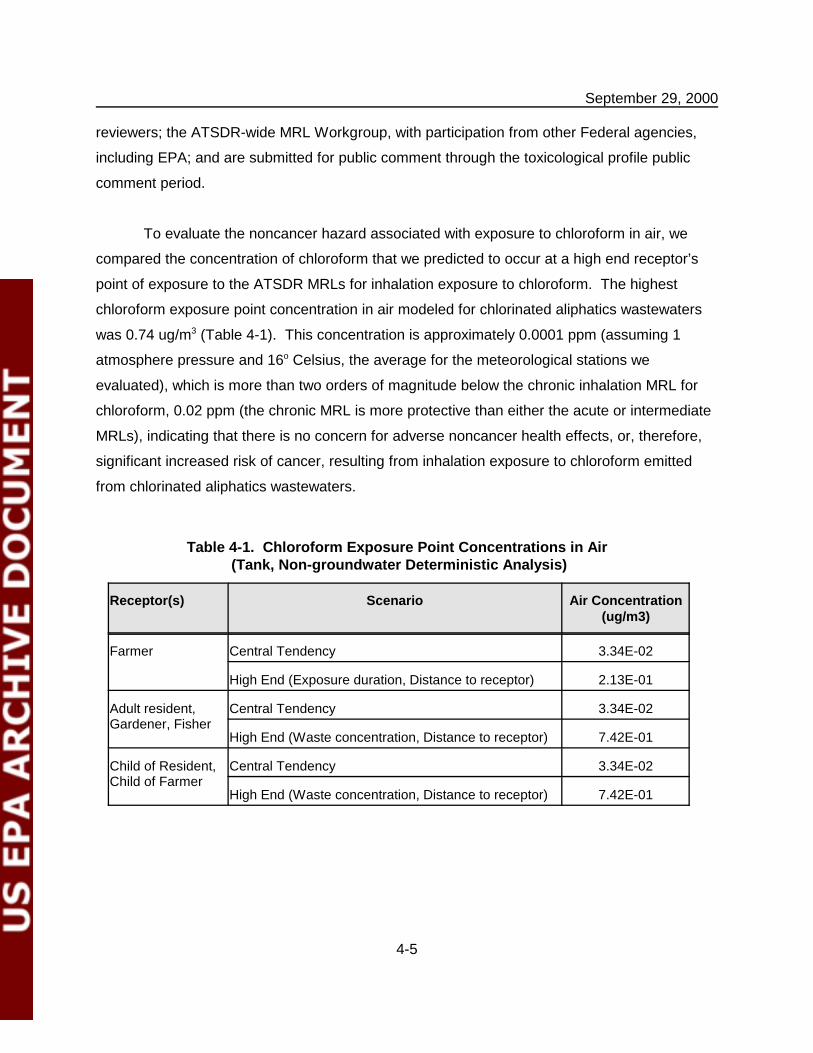
September 29, 2000

4-5

reviewers; the ATSDR-wide MRL Workgroup, with participation from other Federal agencies,

including EPA; and are submitted for public comment through the toxicological profile public

comment period.

To evaluate the noncancer hazard associated with exposure to chloroform in air, we

compared the concentration of chloroform that we predicted to occur at a high end receptor’s

point of exposure to the ATSDR MRLs for inhalation exposure to chloroform. The highest

chloroform exposure point concentration in air modeled for chlorinated aliphatics wastewaters

was 0.74 ug/m3 (Table 4-1). This concentration is approximately 0.0001 ppm (assuming 1

atmosphere pressure and 16o Celsius, the average for the meteorological stations we

evaluated), which is more than two orders of magnitude below the chronic inhalation MRL for

chloroform, 0.02 ppm (the chronic MRL is more protective than either the acute or intermediate

MRLs), indicating that there is no concern for adverse noncancer health effects, or, therefore,

significant increased risk of cancer, resulting from inhalation exposure to chloroform emitted

from chlorinated aliphatics wastewaters.

Table 4-1. Chloroform Exposure Point Concentrations in Air(Tank, Non-groundwater Deterministic Analysis)

Receptor(s) Scenario Air Concentration(ug/m3)

Farmer Central Tendency 3.34E-02

High End (Exposure duration, Distance to receptor) 2.13E-01

Adult resident,Gardener, Fisher

Central Tendency 3.34E-02

High End (Waste concentration, Distance to receptor) 7.42E-01

Child of Resident,Child of Farmer

Central Tendency 3.34E-02

High End (Waste concentration, Distance to receptor) 7.42E-01

September 29, 2000

5-1

5. RISK CHARACTERIZATION


of the 1999 Risk Assessment Technical Background Document. Section 5 of the background

document summarized the deterministic and probabilistic risk analyses for our constituents of

concern and discussed sources of uncertainty in the risk estimates.


• A discussion of the likelihood of noncancer health effects resulting from exposure todioxins in chlorinated aliphatics wastes and an evaluation of dioxin exposure for nursinginfants; and

• A summary of pathway and exposure route-specific land treatment unit TCDD TEQ riskestimates for the adult farmer; and

• A summary of high end risk estimates for chlorinated aliphatics wastewaters andEDC/VCM sludges.

• A revised population risk estimate for the EDC/VCM land treatment unit.

5.1 Non-Cancer Health Effects Resulting from Exposure to Dioxins and Evaluation ofDioxin Exposure for Nursing Infants

Typically, EPA calculates a hazard quotient (HQ) to assess the noncancer health effects

resulting from contaminant exposure. For oral exposures, the HQ is the ratio of an individual’s

daily contaminant dose to the reference dose (RfD) for the contaminant. EPA has not

established RfDs for any of the dioxin or furan congeners (USEPA, 1994). EPA is awaiting the

finalization of the Draft Dioxin Reassessment before formalizing an approach to evaluating

noncancer risks from dioxin. In recent years EPA’s Office of Solid Waste and Emergency

Response (OSWER) has calculated a margin of incremental exposure (MOIE) to dioxin on a

case-by-case basis as a tool for evaluating the potential for the occurrence of noncancer health

effects due to dioxin. The margin of incremental exposure is an expression of the additional

(increment of) exposure to dioxin that an individual receives in excess of background exposure

to dioxin.

September 29, 2000

5-2

Accordingly, we calculated the incremental dioxin exposure for a breast-feeding infant

whose mother’s daily intake of dioxin is 12 pg TCDD International (I)-TEQ, the estimated high

end dioxin daily intake under the adult farmer scenario evaluated in the proposed wastewater

risk analysis (see the revised version of Table 4-4 in the Errata section of this document). The

steps for conducting this calculation are described below.

1. Estimate the TCDD TEQ concentration in the mother’s body fat. We used the

following simple single-compartment, first-order pharmacokinetic model to estimate the TCDD

TEQ concentration in body fat as a function of the intake of dioxins:

Cbf ÿd h CF1

0.693 V CF2

where

Cbf is the TCDD TEQ concentration in body fat (pg/mL fat, or ppt fat)

d is the intake of dioxin (pg/day)

h is the half-life of dioxins in adults (years)

V is the volume of body fat (L)

CF1 is a conversion factor that converts years to days (days/year)

CF2 is a conversion factor that converts L to mL (mL/L).

The values for the variables in this equation are as follows:

Variable Value Units Reference

d, intake of dioxin 12 pg/day Table 4-4, Section 8

h, half-life of dioxins in adults 7.2 years Flesch-Janys et al. (1996) estimated the half-life of 2,3,7,8-TCDD (and other CDD/CDFs) based on blood levels of agroup of occupationally exposed individuals. The medianhalf-life for 2,3,7,8-TCDD (n=48) was estimated to be 7.2years. The value for 2,3,7,8-TCDD is assumed applicable tothe TCDD TEQ.

V, volume of body fat 14 L Assumption. Assuming 1 L = 1 kg, 14 L is 20% of a 70 kgadult.

CF1, conversion factor 365 day/yr

CF2, conversion factor 1000 mL/L

September 29, 2000

5-3

Using these values, we estimate the TCDD TEQ concentration in body fat to be 3.25

pg/mL fat. In Step 2, below, we assume that the TCDD TEQ concentration in the mother’s

body fat is the same as the TCDD TEQ concentration in the mother’s breast milk fat. There are

a number of other uncertainties in the use of this equation, including our assumptions regarding

a 7.2 year half-life for TEQs, the volume of body fat, and the use of a steady state model.

2. Estimate the dioxin dose to the infant. We estimate dose to the infant as:

ADDinfant ÿCmf f3 f4 IRmilk ED

BWinfant AT

where

ADDinfant is the dose to the infant (pg/kg-day)

Cmf is the contaminant concentration in milk fat (pg/mL), assumed to be theconcentration in the mother’s body fat

f3 is the fraction of fat in breast milk (unitless)

f4 is the fraction of ingested contaminant that is absorbed (unitless)

IRmilk is the ingestion rate of milk (mL/day)

ED is the time during with breast feeding occurs, or the exposure duration (yr)

BWinfant is the infant body weight (kg)

AT is the averaging time (yr).

September 29, 2000

4 Schaum et al. (1999) report that “[b]ecause PCB TEQ concentrations in breast milk are similarto those of CDD/Fs, adding the PCB dose from breast milk intake approximately doubles the total TEQdose to infants.”

5 Schaum et al. (1999) report that their results reported as WHO98 TEFs are about 10% greaterthan the same results using the I-TEFs.

5-4

The values for the variables in this equation are as follows:

Variable Value Units Reference

Cmf, contaminant concentration inmilk fat

3.25 pg/g Assumed to be same as TCDD TEQ concentration inmother’s body fat, Cbf, calculated in Step 1

f3, fraction of fat in breast milk 0.04 unitless USEPA, 1997; Table 4-16

f4, fraction of ingested contaminantthat is absorbed

0.9 unitless This assumption is supported by Lakind, et al. (2000),who selected a 95% absorption of 2,3,7,8-TCDD in anursing model for TCDD and cited four studies showingthis much absorption for the lower chlorinated dioxincompounds. Assuming 90% absorption may beconservative for the higher chlorinated dioxins, whichare shown to be excreted at a higher rate.

IRmilk, ingestion rate of breast milk 688 mL/day 12 month time-weighted average mean breast milkintake; USEPA, 1997; Table 4-16

ED, exposure duration 1 yr Assumption, period of time infant is breast-fed

BWinfant, infant body weight 7.2 kg Time weighted average of 50th percentile body weightsfor infants 0-12 months; USEPA, 1997; Table 7-1.Average of values for males and females.

AT, averaging time 1 yr equivalent to exposure duration

With a TCDD TEQ concentration in body fat of 3.25 pg/g (calculated in Step 1), the

dose to the infant is estimated as 11.2 pg/kg-day under the high end wastewater exposure

scenario. Compared to the expected infant background dose of 60 pg TCDD I-TEQ/kg-day due

to exposure to dioxins and furans4 (Schaum et al., 1999; USEPA, 1994), an infant’s high end

indirect exposure to dioxin in chlorinated aliphatics wastewaters represents an incremental

exposure of 19 percent of an infant’s background exposure. EPA also evaluated adult

exposure to dioxin from chlorinated aliphatics wastewaters. Compared to an expected adult

daily background dose of 1 pg TCDD World Health Organization (WHO)-TEQ/kg-day5 due to

exposure to dioxins, furans, and coplanar PCBs (Schaum et al., 1999), the incremental dose

due to chlorinated aliphatics wastewaters, 0.17 pg TCDD I-TEQ/kg-day, is 17 percent of

background. Modifications to EPA’s proposed wastewater risk estimates summarized in

September 29, 2000

5-5

Section 5.3 would result in reducing the incremental exposure for both adults and nursing

infants to less than 10 percent (about 7 percent) of background exposure.

Under the land treatment scenario, the high end adult farmer has a TCDD TEQ intake of

130 pg/day (Table 4-4, USEPA, 1999; Table 4-4, Section 8, this document), or 1.9 pg/kg-day,

which is 186 percent of background exposure. Using the adult’s value for intake, and the

equations in Steps 1 and 2 above, the estimated dose to the infant is 121.1 pg/kg-day.

Compared to the expected infant background dose of 60 pg TCDD I-TEQ/kg-day, an infant’s

high end indirect exposure to dioxin in EDC/VCM sludges managed in a land treatment unit

represents an incremental exposure of 202 percent of an infant’s background exposure.

Modifications to EPA’s proposed EDC/VCM sludge risk analysis summarized in Section 5.3

would result in reducing the incremental exposure for adults to approximately 68 percent of

background and, for nursing infants, to about 74 percent of background exposure.

5.2 Pathway and Exposure Route-Specific Land Treatment Unit TCDD TEQ RiskEstimates for the Adult Farmer

In Appendix H.1 of the 1999 Risk Assessment TBD we provided data for chlorinated

aliphatic wastewaters managed in aerated biological treatment tanks that allowed the reader to

calculate the proportion of the high end deterministic risk for the adult farmer that was due to

the various pathways and route of exposure. We provided similar information for the

EDC/VCM wastewater treatment sludges managed in a land treatment unit, but not in the same

level of detail. Table 5-1 provides a summary of this information for the adult farmer receptor

under the land treatment unit scenario. Some of this information is redundant with

5-6

Table 5-1. TCDD TEQ Risk Results for the Adult Farmer, Land Treatment Unit

Exposure Route and Pathway Percentage of High EndPathway Risk Attributable to:

Percentage of Total Risk Attributable to:

Central Tendency High End

Vegetables (Root and Aboveground)

Erosion and Runoff 63.6 0.3 0.5

Air (Total) 36.4 0.2 0.1

Vapor 33.3

Particulate 3.1

Sum 0.5 0.6

Fruit


Air (Total) 34.7 0.39 0.39

Vapor 33.5

Particulate 1.2

Sum 1.1 1.1

Soil


Air (Total) 2.0 0.05 0.05

Vapor 1.2

Particulate 0.8

Sum 2.2 2.4

Dairy


Air (Total) 70.7 31.8 32.0

Vapor 69.4

Particulate 1.3

Sum 44.8 45.1

Forage 72.6

Grain 0.5

Silage 0.6

Soil 26.3

Beef


Air (Total) 58.0 29.9 29.5

Vapor 56.9

Particulate 1.1

Sum 51.5 50.9

Forage 59.3

Grain 0.1

Silage 0.5

Soil 40.2

September 29, 2000

5-7

the data provided in Table 5-8 of the 1999 Risk Assessment TBD, but is presented again for the

convenience of the reader.

5.3 Summary of High End Risk Estimates – Chlorinated Aliphatics Wastewaters andEDC/VCM Sludges

This section summarizes the how the evaluations and conclusions presented in the

previous sections would influence the risk estimates that we presented in the 1999 Risk

Assessment TBD. Because our listing determinations for chlorinated aliphatic wastewaters and

EDC/VCM sludges managed in a land treatment unit were based primarily on the high end

deterministic dioxin risks for the adult farmer (expressed as TCDD TEQ), and because these

are the highest risks that we identified, the sections below focus on how the factors that reduce

our risk estimates, as highlighted in the previous sections, would influence the deterministic

high end adult farmer dioxin risks.

5.3.1 Chlorinated Aliphatic Wastewaters Managed in Aerated Biological TreatmentTanks

As a result of our analysis of comments provided on the Agency’s Proposed Rule for

chlorinated aliphatics wastes (64 FR 46476), we determined that it was appropriate to adjust

our chlorinated aliphatic wastewater risk assessment results to account for three factors that

were not addressed in the July 1999 risk assessment, and that would reduce our high end

deterministic risk estimate for the adult farmer. These factors are discussed in previous

sections of this document, and are as follows:

• Modifying the assumptions regarding the size of the pasture on which the cattlegraze.

• Accounting for cooking and post-cooking loss of beef.

• Assuming that solids are removed from the wastewater prior to aerated biologicaltreatment

These modifications, and their impact on the proposed risk estimate, are summarized on

the following table (Table 5-2).

September 29, 2000

6 We only calculated the effect of solids removal for ingestion exposures to the dioxinsand furans. The sum of the high end deterministic inhalation risk estimates for the COPCs is9E-07 (including an unadjusted dioxin inhalation risk estimate), and the sum of the high enddeterministic ingestion risk estimates for the COPCs other than dioxins/furans is 2E-09.

5-8

Table 5-2. Modifications to the High End Deterministic Risk Estimate (TCDD TEQ)for the Adult Farmer – Chlorinated Aliphatics Wastewaters

Risk Estimate presented in 1999 Risk Assessment TBD: 2E-05

Modification: New Risk Estimate*:

Assuming farmer only raises beef and dairy cattle 2E-05

Assuming farmer does not provide cattle home-produced grain and silage 2E-05

Accounting for cooking and post-cooking loss of beef 1E-05

Modifying assumptions regarding the pasture size 7E-06

Assuming that solids are removed from the wastewater prior to aeratedbiological treatment

70%Removal

50%Removal

4E-06 6E-06* Each new risk estimate includes the reduction in risk presented in the previous row of the table.

As discussed in Section 4.3, EPA no longer believes there are risks due to exposure to

chloroform derived from chlorinated aliphatics wastewaters. For the adult farmer receptor, the

sum of the inhalation and ingestion deterministic high end cancer risk estimates for the

chlorinated aliphatic wastewater COPCs ranges from 5E-06 to 7E-06, depending on the amount

of solids removal that occurs prior to aerated biological treatment6 (5E-06 corresponds to 70%

solids removal and 7E-06 corresponds to 50% solids removal). The sum of the inhalation and

ingestion deterministic high end noncancer hazard estimates for the chlorinated aliphatic

wastewater COPCs is equal to 0.04. These summed estimates are likely overestimates

because: 1) they are sums of separate high end risk and hazard estimates that may be based

on different high end parameters, thus a number of high end parameters may be combined into

the summed estimate; 2) the cooking and post-cooking loss correction for beef intakes has only

been made for dioxins and furans; 3) the solids removal correction has only been made for

dioxins and furans for ingestion exposures (this correction would be most important for

September 29, 2000

5-9

hydrophobic contaminants); and 4) the pasture/field size correction has only been made for

dioxins and furans.

5.3.2 EDC/VCM Sludges

As a result of our analysis of comments provided on the Agency’s Proposed Rule for

chlorinated aliphatics wastes (64 FR 46476), we determined that it was appropriate to adjust

our land treatment unit risk assessment results to account for three factors that were not

addressed in the July 1999 risk assessment, and that would reduce our high end deterministic

risk estimate for the adult farmer. These factors are discussed in previous sections of this

document, and are as follows:

• Accounting for cooking and post-cooking loss of beef.

• Applying a mass balance correction for the erosion pathway.

• Modifying the assumptions regarding the size of the pasture on which the cattlegraze.

These modifications, and their impact on the proposed risk estimate, are summarized on

the following table (Table 5-3).

Table 5-3. Modifications to the High End Deterministic Risk Estimate (TCDD TEQ)for the Adult Farmer – EDC/VCM Sludges Managed in a Land Treatment Unit

Risk Estimate presented in 1999 Risk Assessment TBD: 2E-04

Modification: New Risk Estimate*:

Assuming farmer only raises beef and dairy cattle 2E-04

Assuming farmer does not provide cattle home-produced grain and silage 2E-04

Accounting for cooking and post-cooking loss of beef 1E-04

Applying a mass balance correction for the erosion pathway 1E-04

Modifying assumptions regarding the pasture size 7E-05* Each new risk estimate includes the reduction in risk presented in the previous row of the table.

September 29, 2000

5-10

For the EDC/VCM landfill nongroundwater pathway analysis, the highest risk estimates

and hazard quotients are associated with the adult farmer receptor. As presented in the 1999

Risk Assessment TBD, the sum of the high end ingestion risk estimates for the adult farmer is

7E-10 and the sum of the high end inhalation risk estimates for the adult farmer is 1E-10, for a

total nongroundwater pathway risk estimate of 8E-10. Nongroundwater pathway hazard

quotients are less than 0.0001 for all contaminants. Our characterization of the high end

groundwater pathway arsenic risk estimate for the farmer, 3E-05 is discussed in the preamble

to the final rule. The sum of all other groundwater pathway risk estimates, regardless of the

timeframe in which the they occur, is only 1E-06. Similarly, the sum of all groundwater pathway

hazard quotients, regardless of the timeframe in which they occur, is only 0.3. Moreover, the

predicted risks for the nongroundwater pathway tend to be overestimates because of the

pasture size and beef ingestion rate assumed in the analysis (described in the preamble to the

final rule), as well as for the reasons described on pages 5-5 and 5-7, and in Appendix H.3, of

the 1999 Risk Assessment TBD. An evaluation of public and peer review comment on the

proposed rule provided no basis for increasing these estimates.

5.3.3 Probabilistic Risk Results

Applying the modifications discussed in the previous sections to our probabilistic risk

estimates is somewhat problematic since the results reported for any one percentile of the

probabilistic distribution are not based on one set of data that can be adjusted in the same way

as we adjusted the deterministic results. However, we assume that there will be the same

general proportion of risk reduction for the probabilistic results as we calculated above for the

deterministic results. In addition, as previously mentioned in Section 2.3, the probabilistic risk

results are probably slightly higher than they would have been if we had evaluated receptor

distances from the source that were more equally distributed.

September 29, 2000

5-11

5.4 Population Risk Estimates

The population risk estimate for the EDC/VCM land treatment unit that EPA presented in

the 1999 Risk Assessment TBD (Section 5.2) was based on an adult beef intake rate that did

not include cooking and post-cooking losses of beef. Because the population risk estimate

was based solely on beef intake, factoring cooking and post-cooking losses of beef into the

population risk estimate would modify the population risk estimate by a factor of 0.55, reducing

the estimate to 9E-05.

September 29, 2000

6-1

6. REFERENCES

Flesch-Janys, D., H. Belcher, P. Gurn, D. Jung, J. Konietzko, A. Manz, and O. Papke. 1996.Elimination of polychlorinated dibenzo-p-dioxins and dibenzofurans in occupationallyexposed persons. Journal of Toxicology and Environmental Health, 47:363-378.

ILSI (International Life Sciences Institute). 1997. An evaluation of EPA’s proposed guidelinesfor carcinogen risk assessment using chloroform and dichloroacetate as case studies:Report of an expert panel. Washington, DC: ILSI Health and Environmental SciencesInstitute. November, 1997.

Jordan, Ellen. 2000. Personal communication with Ann Johnson, EPA Office of Solid Waste,June 26.

Karickhoff, S.W., D.S. Brown, and T.A. Scott. 1979. Sorption of hydrophobic pollutants onnatural sediments. Water Res., v.13, pp. 241-248.

Lakind, J.S., C.M. Berlin, C.N. Park, D,Q, Naiman, and N.J. Gudka. 2000. Methodology forCharacterizing Distributions of Incremental Body Burdens of 2,3,7,8-TCDD and DDEfrom Breast Milk in North American Nursing Infants. Journal of Toxicology andEnvironmental Health, 59:605-639.

Lohman, P.H.M., M.L. Mendelsohn, D.H. Moore II, M.D. Waters, D,J. Brusick, J. Ashby, andW.J.A. Lohman. 1992. A method for comparing and combining short-term genotoxicitytest data: The basic system. Mutat Res 266:7-25 (As cited in ILSI 1997).

Metcalf & Eddy, Inc. 1991. Wastewater Engineering: Treatment, Disposal, and Reuse.Revised by G. Tchobanoglous and F. Burton. Irwin McGraw-Hill, Boston. 1334 pp.(cited elsewhere as Tchobanoglous and Burton, 1991).

Schaum, J., D.L. Winters, L. Phillips, M.N. Lorber. 1999. TEQ doses for CDD/Fs and PCBsgeneral population exposure to dioxin-like compounds in the United States during the1990's. Presented at Dioxin ‘99, the 19th International Symposium on HalogenatedEnvironmental Organic Pollutants and POPs, held September 12-17 in Venice, Italy.Short paper in, Organohalogen Compounds, Volume 44:181-184.

Templin, M.V., J.L. Larson, B.E. Butterworth, K.C. Jamison, J.R. Leininger, S, Mery, K.T.Morgan, B.A. Wong, and D.C. Wolf. 1996a. A 90-day chloroform inhalation study in F-344 rats: Profile of toxicity and relevance to cancer studies. Fund Appl Toxicol 32:109-125.

Templin, M.V., K.C. Jamison, C.S. Sprankle, D.C. Wolf, B.A. Wong, B.E. Butterworth. 1996b.Chloroform-induced cytotoxicity and regenerative cell proliferation in the kidneys andliver of BDF1 mice. Cancer Lett 108:225-231 (As cited in ILSI 1997).

September 29, 2000

6-2

Templin, M.V., K.C. Jamison, D.C. Wolf, K.T. Morgan, B.E. Butterworth. 1996c. Comparisonof chloroform-induced toxicity in the kidneys, liver, and nasal passages of maleOsborne-Mendel and F-344 rats. Cancer Lett 104:71-78 (As cited in ILSI 1997).

Templin, M.V., A.A. Constan, D.C. Wolf, B.A. Wong, B.E. Butterworth. 1998. Patterns ofchloroform-induced regenerative cell proliferation in BDF1 mice correlate with organspecificity and dose-response of tumor formation. Carcinogenesis 19(1):187-193.

Texas A&M. undated. Dairy Cattle. http://asnet.tamu.edu/www/ansc108/labs/Dairy.htm.

Turner, Larry. 1999. Personal communication with Ann Johnson, EPA Office of Solid Waste,December 16.

USEPA (United States Environmental Protection Agency). 1994. Health Assessment for2,3,7,8-TCDD and Related Compounds. Public Review Draft. Office of Research andDevelopment. EPA/600/EP-92/001a-c. September.

USEPA. 1996. Proposed Guidelines for Carcinogen Risk Assessment. 61 FR 17960.

USEPA. 1997. Exposure Factors Handbook, Volumes I, II, and III. EPA/600/P-95/002Fa, b, c.Office of Research and Development, Washington, D.C., August.

USEPA. 1998. Methodology for Assessing Heath Risks Associated with Multiple Pathways ofExposure to Combustor Emissions. National Center for Environmental Assessment.EPA 600/R-98/137. December.

USEPA. 1999. Risk Assessment Technical Background Document for the ChlorinatedAliphatics Listing Determination. July 30.http://www.epa.gov/epaoswer/hazwaste/id/chlorali/clordoc1.htm

WHO (World Health Organization). 1998. Guidelines for Drinking-Water Quality. SecondEdition. Addendum to Volume 2. Health Criteria and Other Supporting Information.Chloroform. pp 255-275. World Health Organization, Geneva.

http://asnet.tamu.edu/www/ansc108/labs/Dairy.htm

http://www.epa.gov/epaoswer/hazwaste/id/chlorali/clordoc1.htm

September 29, 2000

7-1

7. APPENDICES

The following sections present revised versions of four of the Appendices that were

included in the 1999 Risk Assessment TBD. These appendices were revised in response to

comments from peer reviewers who believed that the appendices required additional clarity.

The appendices were not revised to reflect any new analyses or changes in the Agency’s

methodologies that occurred since the 1999 Risk Assessment TBD was completed, only to

provide the clarity and additional detail requested by the peer reviewers. The revised

appendices presented in the following sections are as follows:

• Appendix D.1, Source Term Partitioning Model;

• Appendix D.2, Overland Transport Model;

• Appendix D.4, Groundwater Fate and Transport Modeling Using EPACMTP;

• Appendix D.5, Surface Water Model; and

• Appendix F.1, Monte Carlo Fate and Transport Modeling.

Appendix D.1

Source Term Partitioning Model

September 29, 2000

Appendix D.1 D.1-3

Appendix D.1

Source Term Partitioning Model

This appendix describes the source term partitioning models that were used to estimate

contaminant losses for the following waste management scenarios:

ÿ EDC/VCM sludge managed in onsite land treatment unit (LTU);

ÿ EDC/VCM sludge managed in offsite municipal landfill; and

ÿ Methyl chloride sludge managed in onsite, nonhazardous landfill.

The following discussion describes the general model construct developed to partition chemical

constituents in the waste management unit, and then provides a description of how the general

model was applied to the LTU and landfills, respectively.

Partitioning Model

The source term partitioning model is a time-dependent model that estimates the

contaminant losses from a contaminant source zone (e.g., LTU or landfill) due to volatilization,

leaching, rainwater runoff, and chemical transformation (e.g., biodegradation and hydrolysis).

The model assumes linear partitioning and first order rate losses and uses a finite difference

(numerical) integration approach to solve the mass balance equations. This spreadsheet model

uses the Jury solution (Jury et al., 1983, 1984, and 1990) as the basis for the volatilization flux

calculation. As implemented, the model calculates the average annual contaminant source zone

concentration, the annual mass of contaminant volatilized, and the annual mass of contaminant

removed in the leachate.

September 29, 2000

Appendix D.1 D.1-4

Model Theory

Equilibrium Partitioning

The total concentration of contaminant in the source (i.e., waste unit) can be expressed as

the sum of the concentrations of contaminant adsorbed on the soil or waste particles, dissolved in

the liquid, and in the air spaces as follows:

CT = Cs + (ÿw Cw/�b) + (ÿa Ca/�b) (1)

where

CT = total contaminant concentration (mg/kg = g/Mg)

Cs = concentration of contaminant adsorbed on soil (mg/kg = g/Mg)

ÿw = water-filled soil porosity (m3water/m

3soil)

Cw = concentration of contaminant in liquid (µg/cm3 = g/m3)

�b = soil dry bulk density (g/cm3 = Mg/m3)

ÿa = air-filled soil porosity (m3air/m

3soil)

Ca = concentration of contaminant in air (µg/cm3 = g/m3).

The adsorbed contaminant concentration is assumed to be linearly related to the liquid

phase concentration as follows:

Cs = Kd Cw (2)

where

Cs = concentration of contaminant adsorbed on soil (mg/kg = g/Mg)

Kd =soil-water partition coefficient (cm3/g = m3/Mg) = Koc foc for organic compounds

Koc = soil organic carbon partition coefficient (cm3/g)

foc = organic carbon content of soil (g/g)

September 29, 2000

Appendix D.1 D.1-5

Cw = concentration of contaminant in liquid (µg/cm3 = g/m3).

The contaminant concentration in the vapor phase is assumed to be linearly related to the

liquid phase concentration as follows:

Ca = Hÿ Cw (3)

where

Ca = concentration of contaminant in air (µg/cm3 = g/m3)

Hÿ = dimensionless Henry's law constant = 41 × H

H = Henry's law constant at 25�C (atm-m3/mol)

Cw = concentration of contaminant in liquid (µg/cm3 = g/m3).

Equations 2 and 3 assume linear equilibrium partitioning between the adsorbed

contaminant, the dissolved contaminant, and the volatilized contaminant. Combining

Equations 1, 2, and 3 yields:

CT = Cs [1 + ÿw/(Kd�b) + ÿa Hÿ/(Kd�b)]. (4)

The total contaminant concentration, CT, represents the measured soil concentration.

However, it is the adsorbed soil concentration that is needed to calculate the equilibrium liquid

and air contaminant concentrations (Equations 2 and 3). Equation 4 can be rearranged to

calculate the adsorbed soil contaminant concentration given the total contaminant concentration

as follows:

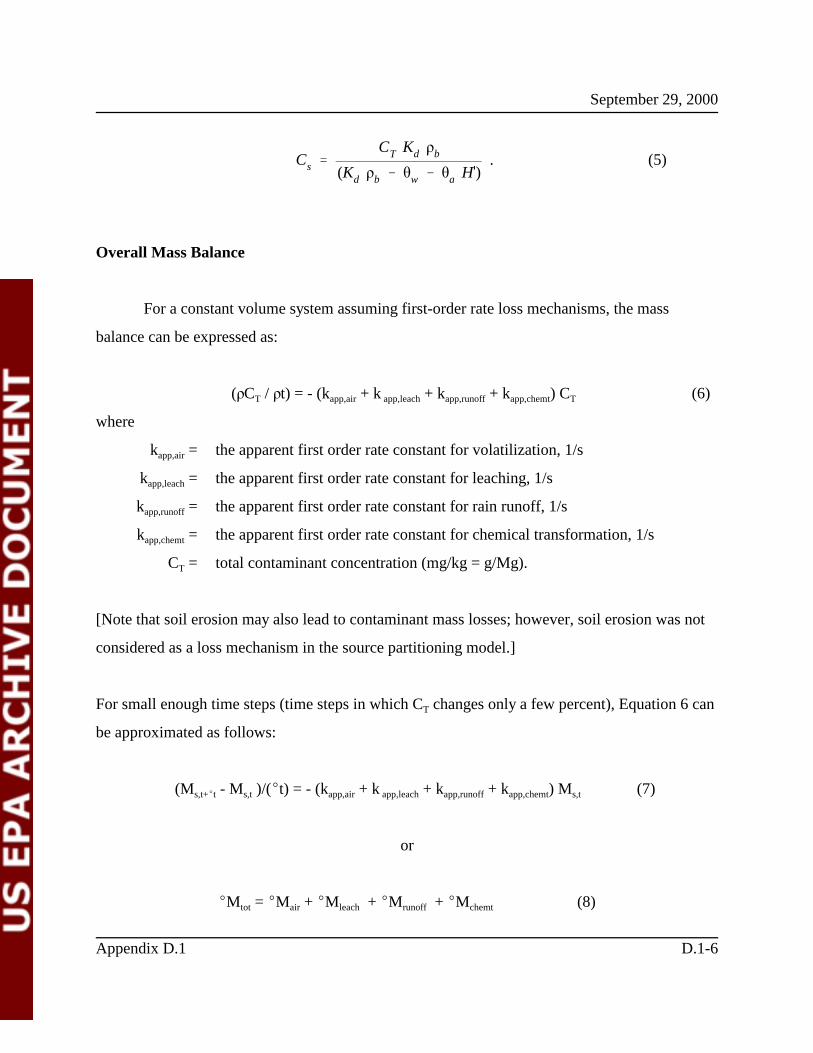
September 29, 2000

Appendix D.1 D.1-6

Cs ÿCT Kd �b

(Kd �b � ÿw � ÿa Hÿ). (5)

Overall Mass Balance

For a constant volume system assuming first-order rate loss mechanisms, the mass

balance can be expressed as:

(�CT / �t) = - (kapp,air+ k app,leach+ kapp,runoff+ kapp,chemt) CT (6)

where

kapp,air= the apparent first order rate constant for volatilization, 1/s

kapp,leach= the apparent first order rate constant for leaching, 1/s

kapp,runoff= the apparent first order rate constant for rain runoff, 1/s

kapp,chemt= the apparent first order rate constant for chemical transformation, 1/s

CT = total contaminant concentration (mg/kg = g/Mg).

[Note that soil erosion may also lead to contaminant mass losses; however, soil erosion was not

considered as a loss mechanism in the source partitioning model.]

For small enough time steps (time steps in which CT changes only a few percent), Equation 6 can

be approximated as follows:

(Ms,t+�t - Ms,t )/(�t) = - (kapp,air+ k app,leach+ kapp,runoff+ kapp,chemt) Ms,t (7)

or

�Mtot = �Mair + �Mleach + �Mrunoff + �Mchemt (8)

September 29, 2000

Appendix D.1 D.1-7

where

Ms,t+�t = mass of contaminant in soil at time t+�t (g)

Ms,t = mass of contaminant in soil at time t (g)

�t = time step of calculation (s)

kapp,air= the apparent first order rate constant for volatilization (1/s)

kapp,leach= the apparent first order rate constant for leaching (1/s)

kapp,runoff= the apparent first order rate constant for rain runoff (1/s)

�Mtot = total mass of contaminant removed from soil over time step (g) = Ms,t - Ms,t+�t

�Mair = mass of contaminant lost over time step due to volatilization (g)

�Mleach= mass of contaminant lost over time step due to leaching (g)

�Mrunoff = mass of contaminant lost over time step due to runoff (g)

�Mchemt= mass of contaminant lost over time step due to chemical transformation (g).

Due to the simplified nature of the numerical integration used, any number of competing loss

mechanisms can be included in the model because each of the loss mechanisms can be evaluated

separately and summed together.

Loss to Atmosphere

The primary mechanism of contaminant loss to the atmosphere is the diffusion of

volatilized contaminant to the soil surface. During periods of evaporation, the flux of water

vapor enhances contaminant transport to the soil surface. Consequently, the total contaminant

flux to the atmosphere is:

Jair,t = Jvol,t + Jevaptr,t (9)

September 29, 2000

Appendix D.1 D.1-8

Jvol,t ÿ CT

0.01 DA

�t

½

1 � exp�d2

s

0.04 DA t(11)

where

Jvol,t = contaminant flux to the atmosphere due to diffusion (g/m2-s)

Jevaptr,t= contaminant flux to the atmosphere due to evaporative transport (g/m2-s).

The total mass loss to the air can be calculated as follows:

�Mair = (Jevaptr,t+ Jvol,t )(A�t). (10)

where

Jevaptr,t= contaminant flux to the atmosphere due to evaporative transport (g/m2-s)

Jvol,t = contaminant flux to the atmosphere due to diffusion (g/m2-s)

A = area of contaminant source (m2)

�t = time step of calculation (s).

The contaminant flux to the atmosphere terms are estimated using the following equations based

on whether the contaminated soil layer is in direct contact with the atmosphere ("no soil cover")

or buried beneath a layer of uncontaminated soil ("soil cover").

Emissions With No Soil Cover

Assuming that there is no soil cover and no stagnant boundary air layer at the ground

surface, the Jury et al. (1990) simplified finite source model for diffusional volatilization can be

written as:

September 29, 2000

Appendix D.1 D.1-9

DA ÿÿ

103

a Di Hÿ � ÿ103

w Dw

n2 (�b Kd � ÿw � ÿa Hÿ)(12)

where


DA = apparent diffusivity (cm2/s)

� = 3.14

t = time (s)

ds = depth of uniform soil contamination at t=0, i.e., depth of daily addition (m).

and

where


3soil)

Di = diffusivity in air (cm2/s)




3soil)

Dw = diffusivity in water (cm2/s)

n = total soil porosity (Lpore/Lsoil) = 1 - (�b/�s)


�s = soil particle density (g/cm3)

Kd = soil-water partition coefficient (cm3/g = m3/Mg) = Koc foc for organic compounds


foc = organic carbon content of soil (g/g).

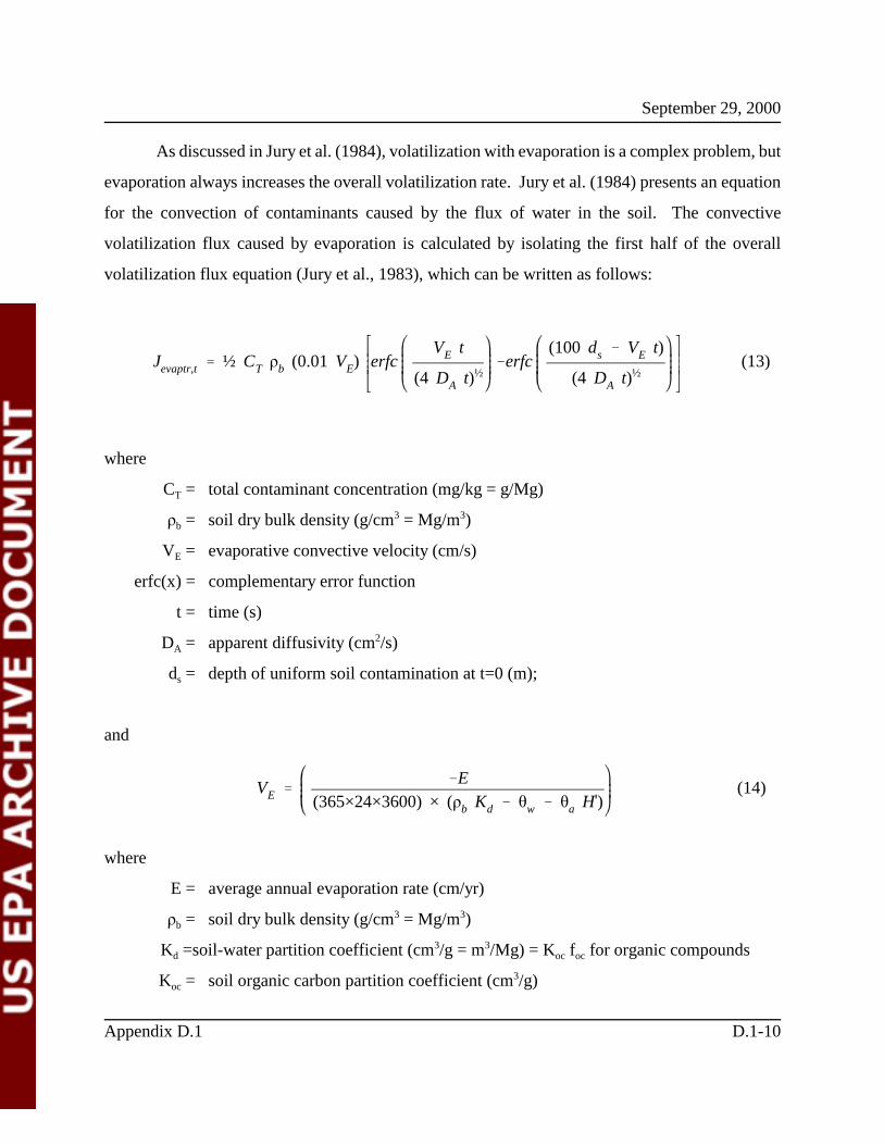
September 29, 2000

Appendix D.1 D.1-10

Jevaptr,t ÿ ½ CT �b (0.01 VE) erfcVE t

(4 DA t)½�erfc

(100 ds � VE t)

(4 DA t)½(13)

VE ÿ�E

(365×24×3600) × (�b Kd � ÿw � ÿa Hÿ)(14)

As discussed in Jury et al. (1984), volatilization with evaporation is a complex problem, but

evaporation always increases the overall volatilization rate. Jury et al. (1984) presents an equation

for the convection of contaminants caused by the flux of water in the soil. The convective

volatilization flux caused by evaporation is calculated by isolating the first half of the overall

volatilization flux equation (Jury et al., 1983), which can be written as follows:

where



VE = evaporative convective velocity (cm/s)

erfc(x) = complementary error function

t = time (s)

DA = apparent diffusivity (cm2/s)

ds = depth of uniform soil contamination at t=0 (m);

and

where

E = average annual evaporation rate (cm/yr)




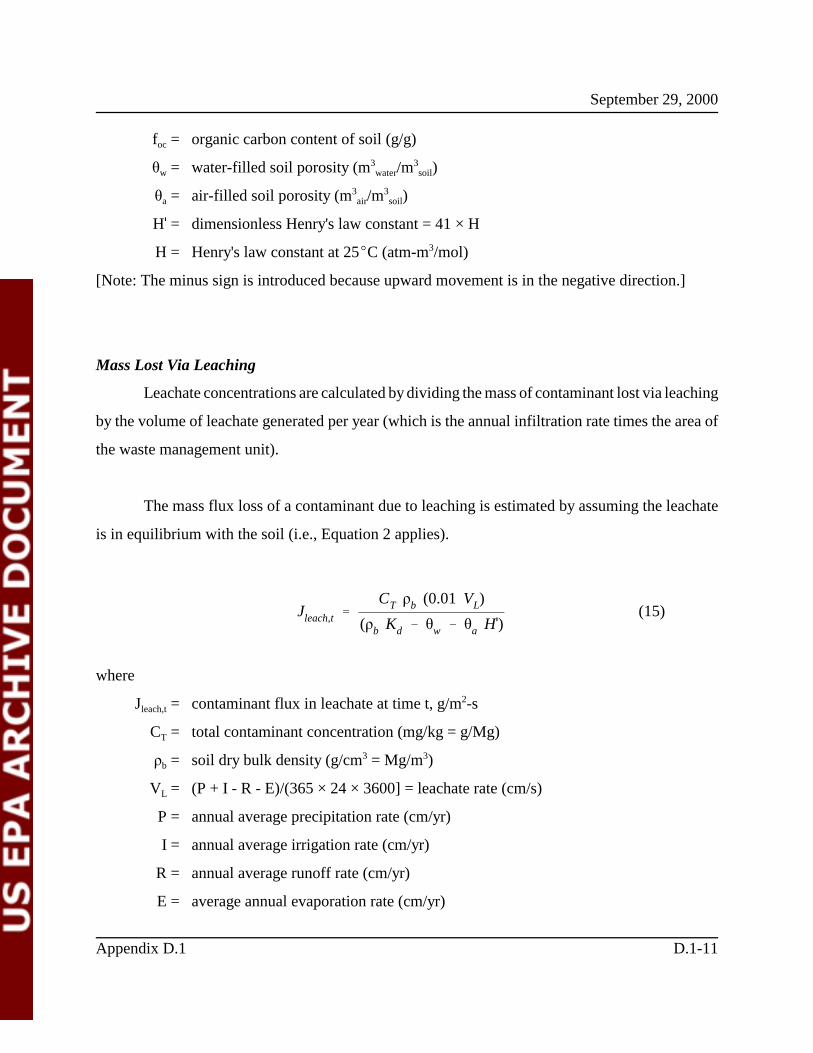
September 29, 2000

Appendix D.1 D.1-11

Jleach,t ÿCT �b (0.01 VL)

(�b Kd � ÿw � ÿa Hÿ)(15)



3soil)


3soil)



[Note: The minus sign is introduced because upward movement is in the negative direction.]

Mass Lost Via Leaching

Leachate concentrations are calculated by dividing the mass of contaminant lost via leaching

by the volume of leachate generated per year (which is the annual infiltration rate times the area of

the waste management unit).

The mass flux loss of a contaminant due to leaching is estimated by assuming the leachate

is in equilibrium with the soil (i.e., Equation 2 applies).

where

Jleach,t= contaminant flux in leachate at time t, g/m2-s



VL = (P + I - R - E)/(365 × 24 × 3600] = leachate rate (cm/s)

P = annual average precipitation rate (cm/yr)

I = annual average irrigation rate (cm/yr)

R = annual average runoff rate (cm/yr)

E = average annual evaporation rate (cm/yr)

September 29, 2000

7 During the development of the model, we reviewed the assumption that runoff is in equilibrium with thesoil. Because data on storm events and rain intensity would be required to evaluate nonequilibrium runoff, we didnot attempt to define the proportion of runoff that enters the soil (versus that which does not). The runoff thatcauses soil erosion would mix well with the eroding soil particles, some of which may be redeposited on the LTU.Consequently, even the runoff that does not enter the soil will contain some contaminant. Given the mathematicalconstruct used to estimate contaminant partitioning in soil, and data availability on precipitation, evaporation, andrunoff, assuming equilibrium conditions was considered the most technically defensible option.

Appendix D.1 D.1-12

Jrunoff,t ÿCT �b (0.01 VR)

(�b Kd � ÿw � ÿa Hÿ)(17)

Kd = soil-water partition coefficient (cm3/g = m3/Mg) = Koc foc for organic compounds




3soil)


3soil)



In the same fashion that the air fluxes were converted a mass loss, the leaching flux rate can

be converted to a mass loss as follows:

�Mleach= (Jleach,t)(A�t). (16)

Loss Due to Runoff

The equation describing the mass flux loss of a contaminant due to runoff is nearly

identical to Equation 15, because the runoff is also assumed to be in equilibrium with the

contaminated soil.7 Consequently, the total mass rate of contaminant loss due to runoff is

where

Jrunoff,t = contaminant runoff rate at time t (g/m2-s)

September 29, 2000

Appendix D.1 D.1-13



VR = R/(365 × 24 × 3600] = runoff rate (cm/s)





3soil)


3soil)



Then,

�Mrunoff = (Jrunoff,t)(A�t). (18)

Loss Due to Chemical Transformation

Chemical transformation (e.g., biodegradation and hydrolysis) rates were imputed from

reported contaminant half-lives in soil. The contaminant half-life was used to calculate an

overall first order rate constant that included all loss mechanisms. Then the total mass loss

predicted from this overall first order rate constant was calculated as follows:

�Mtot = Ms,t [1 -exp(- kapp,overall�t)] (19)

where

�Mtot = total mass of contaminant loss from the system (g)

Ms,t = mass of contaminant in soil at time t (g)

kapp,overall= overall apparent first order rate constant for contaminant loss by all mechanisms(1/s)

�t = time step of calculation (s).

September 29, 2000

Appendix D.1 D.1-14

If �Mtot exceeds the mass losses from volatilization, leaching and runoff, then the

additional mass loss was attributed to (biodegradation+hydrolysis). If the volatilization, leaching

and runoff mass losses exceeded�Mtot, then the mass chemically transformed was set to zero.

Application of Model to Land Treatment Unit

In applying the general model to the LTU, we made certain simplifying assumptions.

First, we assumed the contaminant source zone is a thoroughly mixed system and, therefore, a

concentration profile is not developed over the depth of the zone. Second, we assumed that the

contaminant losses due to erosion of soil particles could be neglected without serious

implications with regard to mass balance of contaminant. Although it has been shown that

organic contaminants tend to sorb to soil fines, and that fine particles of soil tend to erode

readily, we accept this limitation and acknowledge that there may be a slight overestimation of

the leachate and atmospheric flux because contaminant losses from eroded soil particles are not

explicitly accounted for.

Under this waste management scenario, we assumed that the LTU operates for 40 years

with annual waste applications (i.e., one application per year). At the end of 40 years, the LTU

ceases to receive EDC/VCM sludge, but it may potentially continue to release contaminants into

the environment. Therefore, the model tracks the average annual soil concentration, leachate

concentration, and the annual mass of contaminant volatilized for the 40 years of active use as

well as the period of 40 years of inactive use after the LTU ceases operations (i.e., no additional

waste applications). The maximum nine-year leachate concentration predicted by the model is

delivered to the groundwater model and used as the starting leachate concentration for the

groundwater simulation. The post-closure period of 40 years was used to ensure that the

maximum nine-year average leachate concentration is captured over the simulation.

September 29, 2000

Appendix D.1 D.1-15

Land treating often involves tilling the waste into the soil. We assumed that the

EDC/VCM sludge is tilled to a depth of 0.2 m (U.S. EPA, 1990). We also assumed that there

were no runoff/runon controls in place at the LTU to mitigate the release of contaminants via

runoff.

The total mass of contaminant applied to the soil during the first annual application can

be calculated as follows:

Ms,app= (CT Qapp) × 1-yr (20)

where

Ms,app= mass of contaminant in soil from waste application (g)


Qapp = annual waste application rate (Mg/yr).

Modeling time-steps for the LTU were set equal to 1 day. After each time step, the mass

of constituent remaining in the soil was calculated. We assumed that the contaminant

concentrations were uniform over the tilling depth at the beginning of each time step. The model

does not generate source zone concentration profiles over time (as a function of depth) given our

assumption that active land treatment units are tilled regularly.

Mass additions to the system occur during waste application. The depth of material

added during an application is generally negligible; however, some model scenarios could have

significant waste material accumulation over 40 years depending on the tilling depth, application

rate, and other factors. As waste is sequentially added, and given a fixed tilling depth, a small

layer of contaminated soil at the bottom of the land treatment unit will not be tilled in with the

newly added waste. The thickness of this layer is equal to the effective thickness of the applied

waste (i.e., the volume of the applied waste divided by the surface area of the unit). This layer at

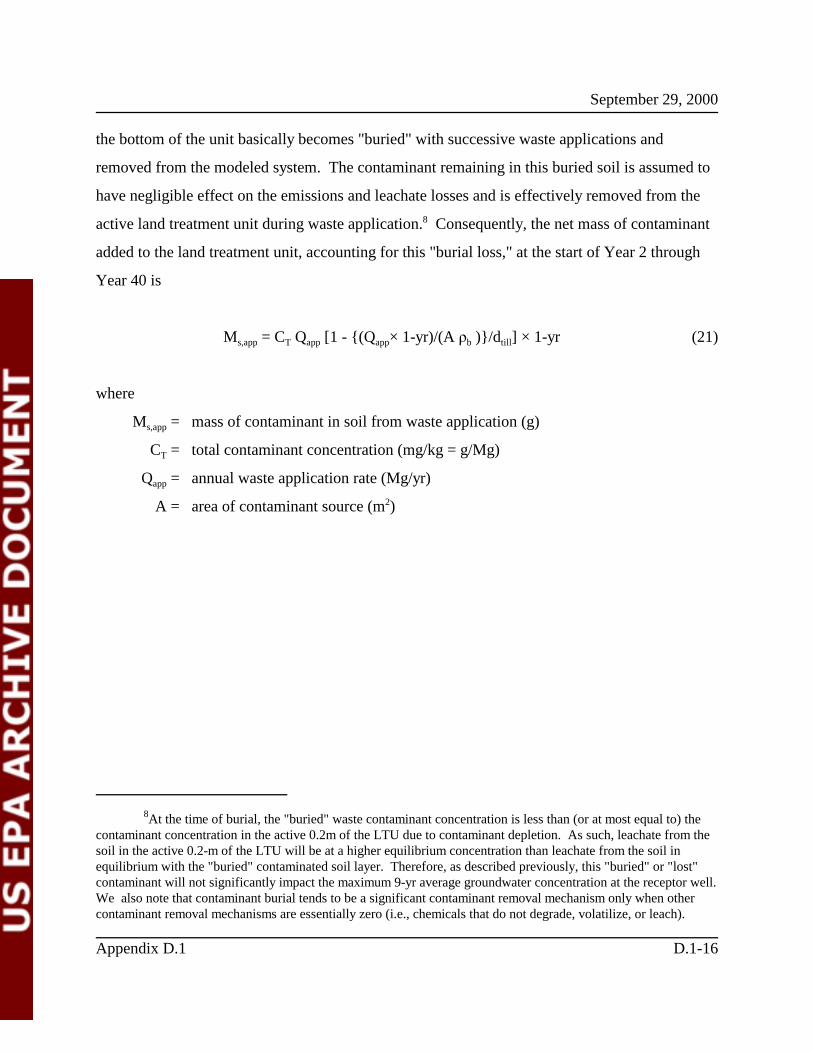
September 29, 2000

8At the time of burial, the "buried" waste contaminant concentration is less than (or at most equal to) thecontaminant concentration in the active 0.2m of the LTU due to contaminant depletion. As such, leachate from thesoil in the active 0.2-m of the LTU will be at a higher equilibrium concentration than leachate from the soil inequilibrium with the "buried" contaminated soil layer. Therefore, as described previously, this "buried" or "lost"contaminant will not significantly impact the maximum 9-yr average groundwater concentration at the receptor well.We also note that contaminant burial tends to be a significant contaminant removal mechanism only when othercontaminant removal mechanisms are essentially zero (i.e., chemicals that do not degrade, volatilize, or leach).

Appendix D.1 D.1-16

the bottom of the unit basically becomes "buried" with successive waste applications and

removed from the modeled system. The contaminant remaining in this buried soil is assumed to

have negligible effect on the emissions and leachate losses and is effectively removed from the

active land treatment unit during waste application.8 Consequently, the net mass of contaminant

added to the land treatment unit, accounting for this "burial loss," at the start of Year 2 through

Year 40 is

Ms,app= CT Qapp [1 - {(Qapp× 1-yr)/(A �b )}/dtill ] × 1-yr (21)

where

Ms,app= mass of contaminant in soil from waste application (g)


Qapp = annual waste application rate (Mg/yr)

A = area of contaminant source (m2)

September 29, 2000

9 As indicated in the discussion of the general model, the calculations for volatilization fluxes are basedon the Jury solution.

Appendix D.1 D.1-17


dtill = tilling depth = 0.2 m.

Application of Model to Landfills

In applying the general partitioning model to the landfill, we make certain simplifying

assumptions. First, although the closed landfill cells consist of two layers (i.e., a waste zone and

cap zone), application of the Jury solution to predict volatilization from the landfill requires that

the soil properties are homogenous in both zones.9 Consequently, the model does not recognize

differences in permeability between the two layers (as a function of density, void fraction,

organic content). The contaminant source model does, however, account for the difference in

concentrations between the waste zone and cap zone (e.g., the initial contaminant concentration

in the cap zone is set to zero). In addition, the source partitioning modeldoesproduce a

concentration profile over depth (one of the benefits of applying the Jury solution). However, the

contaminant fluxes are based on total mass in the contaminant source zone and, therefore, the

concentration profile is not required by the air dispersion model. Second, the mass of constituent

predicted to volatilize by the source partition model was assumed to reduce the total mass of

constituent in the landfill available for leaching. Therefore, the total mass volatilized is

subtracted from the total mass of constituent placed in the landfill, and this reduced mass is

assumed to be the mass of constituent that may be depleted during the life of the simulation (due

to leaching). Lastly, no hydrolysis or biodegradation is assumed to occur in the landfill.

Under this waste management scenario, the model was used to evaluate volatilization

from the landfill for three conditions. The first condition is the daily waste addition in which the

waste is in direct contact with the atmosphere. The second condition is the active landfill cell in

September 29, 2000

10 For municipal landfill analyses, TCLP data are used in preference to modeled leachate data as a matterof U.S. EPA policy.

Appendix D.1 D.1-18

which the waste is covered by a thin "daily" cover. The third condition is the closed landfill cell

in which the waste is covered by a thick landfill cap. The source partitioning model was used to

estimate the mass of constituent volatilized from the waste, as well as the mass of constituent that

leaches from the contaminant source zone. However, the groundwater modeling simulation of

the landfill did not use the leachate flux predicted by the source partitioning model. Instead, the

landfill leachate concentration from the Toxicity Characteristic Leaching Procedure (TCLP) data

was used as the starting leachate concentration.10 This approach is consistent with the source

partitioning model except that TCLP data were to determine the initial leachate concentration

rather than deriving an initial leachate concentration using a partition coefficient that describes

the relationship between total waste and liquid-phase concentration (as described by Equation 2).

In short, the leachate flux was included in the source partition model to account for the fact that

leaching may be a competitive removal mechanism to volatilization for certain chemicals.

For the chlorinated aliphatics listing determination, two landfill scenarios were modeled.

ÿ EDC/VCM Sludge Offsite Municipal Landfill - We assumed that EDC/VCM

sludges are disposed in offsite in unlined municipal landfills. Based on municipal

solid waste management requirements (40 CFR Part 258), we assumed that the

landfills are covered daily (every 12 hours) with soil and are capped at the end of

their active life, which is 30 years (30 years is the average active lifetime of

municipal Subtitle D landfills based on a survey conducted by EPA [U.S.EPA

1988]). We assumed that the landfill continues to release contaminants into the

environment for 40 years after it is closed.

ÿ Methyl Chloride Sludge Onsite Nonhazardous Landfill - Review of the §3007

survey responses found that methyl chloride sludge is managed at a single facility in

September 29, 2000

Appendix D.1 D.1-19

a landfill that is lined with a 24-inch clay liner and has a leachate collection system.

We estimated that the landfill would have an active life of 90 years. We assumed

that the landfill continues to release contaminants into the environment for 40 years

after it is closed.

The waste added to the landfill was assumed to be homogeneous with respect to the

concentration throughout the waste as well as the concentration in each waste addition over time.

One landfill cell was assumed to be filled per year. The user enters the annual waste quantity and

the contaminant concentration of the waste of interest, the waste density, the dimensions of the

entire landfill, and the life expectancy of the landfill. From this information, the dilution effect

of the target waste being added to other waste in the landfill was calculated. The partitioning

equations were applied in three distinct compartments to the landfill model. These included the

daily waste addition in which the waste is in direct contact with the atmosphere, the active

landfill cell in which the waste is covered by a thin "daily" cover; and the closed landfill cell in

which the waste is covered by a thick landfill cap.

Losses from the active landfill cell were estimated by simulating the addition of waste to

the landfill on a daily basis. It was assumed that a daily waste addition was 2.5 feet deep and its

volume was determined by the annual waste disposal rate, assuming 350 operating days per year.

The waste was assumed to be uncovered in the landfill for a user-specified time (model runs

were made using an uncovered duration of 12 hours). After the initial uncovered 12 hours, a

6-inch thick cover was added to the waste daily. It was assumed that the daily waste additions

were disposed of so that the landfill was filled in layers, with the entire first layer of the cell

being filled first, then the second layer was filled in the same order as the first layer, and so on.

The total amount of contaminant emitted and leached from the landfill cell was calculated by

modeling these individual daily waste additions and summing the results for each waste addition.

September 29, 2000

Appendix D.1 D.1-20

CL(t) ÿ C 0L e

�VL

d Fh �b (C0T/C 0

L)t

(22)

After an active landfill cell was completely filled (it was assumed that it took 1 year to fill

each cell), the landfill cell was capped. Losses from the entire landfill were estimated by

simulating the sequential filling of landfill cells. For example, in Year 1, there were losses from

an active cell. In Year 2, there were losses from an active cell plus losses from the first year of a

capped cell. In Year 3, there were losses from an active cell plus losses from two capped cells,

and so on. Once the entire landfill was filled, the model simulated 30 closed cells from Year 31

to the end of the simulation period.

As indicated above, the landfill leaching losses were estimated using a source partitioning

module inside the EPACMTP subsurface fate and transport model (see Appendix D.4 for

additional details on the groundwater modeling). The TCLP test is designed to simulate landfill

leachate and use of these measured values was deemed appropriate to model the landfill leaching

process. Using both the measured waste concentration (CT) and TCLP leachate concentration

(CL0), the time-dependent leachate concentration, CL(t), is given by:

where

d = Landfill depth (m)

Fh = Volume fraction of the landfill occupied by the waste

CL0 = Initial leachate concentration (equal to measured TCLP concentration) (mg/L)

CT0 = Initial total waste concentration (mg/kg)

t = time (yr)

This equation does not set a leaching perioda priori; rather, the leaching process continues until

all constituent mass in the landfill has been depleted. During the leaching process, the

September 29, 2000

Appendix D.1 D.1-21

constituent concentration remaining in the landfill is gradually depleted, and the resulting

leachate concentration also diminishes with time following the exponential relationship

expressed by Equation 22 (USEPA, 1996). The superscript0 in this equation is used to denote the

initial concentration in the waste at the beginning of the leaching process (CT0), and the initial

leachate concentration, CL0, where the latter is given by the measured TCLP concentration. In

order to ensure a correct accounting for the total amount of constituent disposed in the landfill, as

well as the mass lost via volatilization, the assumption was made that leaching does not begin

until the landfill is closed, i.e, Fh in Equation 22 represents the amount of waste when the landfill

is “full.” The initial waste concentration, CT0 is determined from the waste concentration

entering the landfill after adjusting for the mass lost due to volatilization during the landfill

active life. As noted above, the source partitioning model was used to calculate the mass lost to

volatilization. In modeling the landfill leaching process, additional volatilization losses that may

occur after landfill closure are ignored based on the assumption that volatilization losses will be

minor following placement of the final landfill cap. This assumption may overestimate the

amount of constituent which is available for leaching as it ignores volatilization losses that occur

after landfill closure. Note that for the purposes of determining exposures and risk via the

atmospheric pathway described previously, volatilization losses for 40 years following closure

were modeled.

References

Jury, W.A., W.F. Spencer, and W..J. Farmer. 1983. Behavior assessment model for traceorganics in soil: i. model description.J. Environ. Qual.12(4):558-564.

Jury, W.A., W..J. Farmer, and W.F. Spencer. 1984. Behavior assessment model for traceorganics in soil: ii. chemical classification and parameter sensitivity.J. Environ. Qual.13(4):567-572.

Jury, W.A., D. Russo, G. Streile, and H.E. Abd. 1990. Evaluation of volatilization by organicchemicals residing below the soil surface.Water Resources Research.26(1):13-20.

September 29, 2000

Appendix D.1 D.1-22

U.S. EPA. 1988. National Survey of Solid Waste (Municipal) Landfill Facilities. EPA/530-SW-88-034. Office of Solid Waste, Washington, DC. September.

U.S. EPA. 1990. Methodology for Assessing Health Risks Associated with Indirect Exposure toCombustor Emissions - Interim Final. EPA/600/6-90/003. January.

U.S. EPA. 1994b. Criteria for Municipal Solid Waste Landfills (Eff. 10-9-93).Code of FederalRegulations40 CFR 258.

U.S. EPA (U.S. Environmental Protection Agency). 1996. EPA'sComposite Model for LeachateMigration with Transformation Products (EPACMTP) Background Document for theFinite Source Methodology. Office of Solid Waste, Washington, DC.

Appendix D.2

Overland Transport Model

September 29, 2000

Appendix D.2 D.2-3

Appendix D.2

Overland Transport Model

Conceptual Approach to Modeling Overland Transport

The overland transport of contaminants was considered a potentially important

mechanism by which constituents in chlorinated aliphatics wastes may be released from a land

treatment unit (LTU), and contaminate environmental media and food to which humans may be

exposed. Consequently, an overland transport model was developed to predict the erosion losses

from the LTU and the resulting contaminant load to a receiving waterbody and the intervening

area between the LTU and the waterbody. The Universal Soil Loss Equation (USLE) was chosen

as the construct to predict erosion losses from the LTU. The USLE is an empirical erosion

model and constitutes a standard tool for exposure assessment involving overland pathways.

This empirical model was developed to estimate long-term average soil erosion losses to a nearby

waterbody from an agricultural field having uniform slope, soil type, vegetative cover, and

erosion-control practices. It is important to recognize that, for this analysis, the USLE was not

modified to calculate the unit soil loss rate; rather, the application of USLE in the overland

transport model was modified by introducing the concept of soil mass balance within an

integrated drainage subbasin consisting of the LTU, the receiving field (e.g., agricultural field)

and surrounding buffer areas. The sediment delivery ratio, defined by empirical data on sediment

delivery from drainage basins to receiving streams, was assumed to be constant throughout this

integrated setting and used to estimate the fraction of eroded soil (and contaminant) that

ultimately reached the field; the soil (and contaminant) that did not reach the waterbody was

September 29, 2000

Appendix D.2 D.2-4

assumed to be evenly redeposited in the drainage subbasin. Therefore, instead of estimating the

soil (and contaminant) load from the LTU to the water body as the USLE soil loss rate times the

LTU area, the load was calculated as the USLE soil loss rate times the LTU area times the

sediment delivery ratio.

This conceptual approach was first described in Beaulieu et al., 1996, and represented a

method to evaluate erosion processes within an integrated setting. Because the USLE equation

estimates only soil erosion to waterbodies, the receptor location (i.e., the receiving field) must be

located between the LTU and the waterbody. In summary, the equations derived to predict

erosion in the integrated setting are based on the following assumptions:

ÿ The area of the management unit (LTU) and the area between the management unit

and the nearest waterbody, including the receptor site, make up a discrete drainage

subbasin.

ÿ The sediment delivery ratio (SDSB) and the soil loss rate per unit area are assumed to

be constant for all areas within the subbasin.

ÿ The amount of soil deposited onto the receptor site through soil erosion is estimated

by assuming that the fraction of soil that does not reach the waterbody remains in the

subbasin.

ÿ The entire subbasin drainage system is assumed to be at steady-state. Consequently,

steady-state soil concentrations for the different subareas (e.g., receptor site,

surrounding area) can be calculated using a mass balance approach.

ÿ The soils within the subbasin are assumed (on the average) to have the same soil

properties (e.g., bulk density, soil moisture content).

September 29, 2000

Appendix D.2 D.2-5

ÿ No contributions to constituent concentrations are assumed to occur from sources

other than the LTU within the subbasin.

Background to the Overland Transport Model

The USLE equation contains several factors that influence the amount of soil that is

eroded from a site. These factors are all multiplied together to estimate the unit soil loss rate (the

amount of sediment that erodes per unit area per unit time) and include:

ÿ rainfall (or erosivity) factor, 1/yr

ÿ erodibility factor, ton/acre

ÿ length-slope factor

ÿ cover management factor

ÿ supporting practice factor.

Researchers have observed that the bulk of eroded sediment is deposited at intermediate

locations wherever the entraining runoff waters are insufficient to sustain transport. This effect

was quantified as described by Vanoni (1975) using a regression model of the form SD = aAb,

where A is the drainage area. The sediment delivery ratio (SD) reflects the empirical observation

that the rate of soil erosion observed on small areas (as estimated by the USLE) is diminished as

one considers larger and larger areas.

A single sediment delivery ratio was calculated based on the area of the subbasin. That

sediment delivery ratio was then assumed to apply to any hypothetically defined subarea within

the subbasin, and this was referred to as the "fixed sediment delivery ratio." Although the

sediment originating in areas further away from the receiving waterbody would have more

opportunity to settle (and, therefore, are less likely to reach the waterbody) than sediment

September 29, 2000

Appendix D.2 D.2-6

originating in areas directly adjacent to the waterbody, we adopted a simplifying assumption of a

fixed sediment delivery ratio for all subareas within the subbasin for two reasons.

First, using the "fixed" sediment delivery ratio for each subarea forced the summation of

subarea sediment loads to equal the total sediment load to the receiving waterbody as estimated

using the Vanoni correlation for the entire drainage subbasin. Due to the non-linearity of the

Vanoni equation, separate application of the equation to the subareas yielded total sediment loads

to the waterbody that were different than the sediment load predicted based on the subbasin area.

Clearly, the derivation of the empirical relationship presented by Vanoni does not provide the

level of resolution necessary to discretize the drainage subbasin into independent drainage

subareas. Moreover, the mathematical solution needed to implement such an approach would

have required integration of all subareas within the drainage subbasin (e.g., soil movement into

and out of each subarea) to ensure that the total soil load to the waterbody matched the

summation of the individual loads.

Second, the fixed sediment delivery ratio provides a reasonable estimate of the

contaminant load to the receiving waterbody (or stream). This estimate is likely to be somewhat

conservative because: 1) the LTU is expected to contribute eroded sediment with the highest

contaminant concentration; and 2) the LTU is further away from the receiving waterbody. As the

source is the further from the receiving waterbody than the receiving field, soil eroded from the

source would have more opportunity to settle in the intervening areas than soil from areas closer

to the waterbody (e.g., the field). Therefore, the fixed sediment delivery ratio is expected to

provide a reasonably conservative estimate of amount of sediment that erodes directly from the

source and reaches the waterbody.

The soil erosion model uses the average soil concentration as calculated for the land

treatment unit (LTU) by the source partition model (see Appendix D.1 for detailed description of

the source partition model). The overland transport model then assumes that the concentration in

September 29, 2000

Appendix D.2 D.2-7

the LTU remains constant for the period of time that it takes for the intervening and receiving

fields to reach a steady-state concentration. However, the LTU typically has a finite life, and

therefore, it is a finite source of contaminated sediment. Time-dependent analysis that were

performed under similar modeling exercises suggested that roughly 50 years are needed for the

intervening area and receiving field soils to approach steady-state concentrations. Because the

contaminant concentration in the LTU will decrease with time (as contaminant mass is eroded),

fixing the LTU concentration given the steady-state assumption will tend to produce an

overestimate of the contaminant load to both receiving fields and the waterbody. This is a source

of uncertainty and a limitation of the current construct.

Site Layout for Modeling the Overland Transport

The Equations shown in Table E-1.5 (as well as the equations in Tables E-1.9 and E-1.29)

describe the site geometry of the waste management unit (WMU), field (i.e., receptor site), and

receiving waterbody. Implicit in these equations are two simplifying assumptions regarding the

relative areas considered in the modeling overland transport. First, the WMU (i.e., the

contaminant source) and agricultural field are assumed to be square. Second, the intervening

area (defined as the region between the source and the waterbody) is assumed to be at least as

large as the source. Therefore, two basic scenarios exist:

1) the source is larger than the receptor field (Figure 1); and

2) the receptor field is larger than the source (Figure 2).

Thus, if the waste management unit (WMU) is larger than the source, the intervening area

consists of the field and a buffer that is square and equal in size to the WMU. Conversely, if the

WMU is smaller than the field, the field constitutes the intervening area and the up-slope area

consists of the WMU and a buffer that is square and equal in size to the field. Given these

September 29, 2000

Appendix D.2 D.2-8

Figure 2. Field > Source.

Figure 1. Source > Field

September 29, 2000

Appendix D.2 D.2-9

DS0,F ÿ Xe × As × (1�SDSB) × SF0,F(D-1)

assumptions illustrated in Figures 1 and 2, the equations derived to estimate for the areas of the

buffer and surrounding areas are straightforward, involving simple geometry.

Soil Load from LTU to Receiving Field

The mass of eroded soil (soil load) from the LTU to the receptor site (SLO,F) is a major

input required to calculate the receptor site soil constituent concentration (CF). The receptor site

(residential plot, home garden, or agricultural field) soil concentrations are used to estimate risk

through the soil ingestion pathway for all scenarios and through the food chain pathways (e.g.,

above-ground and below-ground produce) for the home gardener and farmer scenarios.

Assuming that the probability that soil from the LTU is transported and deposited is equivalent

for the intervening area and receptor site, the amount of contaminated soil that leaves the source

area can be calculated by using a simple ratio of the area of concern to the total area for soil

deposition:

where

DS0,F = soil delivery rate from source (LTU) to receptor (kg/yr)

Xe = unit soil loss rate from LTU (kg/m2/yr)

AS = area of the LTU (m2)

SDSB = sediment delivery ratio of the subbasin to the nearest waterbody

(unitless)

SF0,F = deposition area scaling factor (m2/m2)

= ratio of the receiving field area to the entire area available for deposition

= AF/(AS + AB/Surr + AF)

September 29, 2000

Appendix D.2 D.2-10

AF = area of the receiving field (m2)

AB/Surr = area of the buffer and surrounding areas within the subbasin (m2).

The sediment delivery ratio (SD) provides an estimate of the fraction of the mobile

sediment that directly reaches the waterbody. Consequently, 1- SD provides an estimate of the

amount of sediment that does not reach the waterbody and must, therefore, be redeposited in the

intervening areas. As suggested previously, the SD reflects the empirical observation that the

rate of sediment reaching the stream due to soil erosion observed on small areas (as estimated by

the USLE) is diminished as one considers larger and larger areas. Larger drainage basins, which

have areas that are further from the receiving waterbody, typically have a lower sediment

delivery ratio than smaller drainage basins. Specifically, researchers have observed (from TSS

measurements in streams) that “The bulk of the sediment is deposited at intermediate locations

wherever the entraining runoff waters are insufficient to sustain transport. It is scattered to

adjacent downslope positions; it is deposited at the base of eroding slopes; ...” (Vanoni, 1975).

This effect was quantified as described by Vanoni (1975) using a regression model of the form

SD = aAb, where A is the drainage area. Using field data from a number of sources that cover a

large range of drainage area sizes, researchers estimated the "a" and "b" parameters to be those

values such as are used in our model. As seen in Appendix E,Table E-1.4, b=-1/8 and "a" is

dependent on the drainage (i.e., subbasin) area.

Because the USLE requires the assumption of homogeneity throughout the basin, and in

view of the fact that the SD is not intended to resolve erosion of soil particles by distance from

the waterbody, the sediment delivery ratio is assumed to be constant for the drainage subbasin

consisting of the LTU, field, and buffer areas. Although the use of the SD does not capture storm

events, the model does predict that the majority of the sediment that erodes from the LTU

directly reaches the stream, effectively averaging the erosion losses over storm events ranging

from mild to severe. In short, the SD reflects annual average sediment transport and was chosen

as the most appropriate tool to estimate the long-term sediment yields to the stream based on

September 29, 2000

11 Pervious runoff refers to runoff from watershed soils that are subject to infiltration. Impervious runoffrefers to runoff from watershed areas closed to infiltration, such as paved roads. The drainagesubbasin was assumed to consist exclusively of pervious soils.

Appendix D.2 D.2-11

field measurements. The sediment delivery ratio (SD) is used to estimate how much of the

eroding soil reaches the waterbody, and 1-SD is used to estimate how much of that soil is

redeposited in the area between the LTU and the receiving stream.

Uniform or even redeposition of sediment is a simplifying assumption used in the model

construct; no other assumption appeared technically defensible within the confines of a

spreadsheet model. Flow channeling or uneven redeposition could cause all, none, or any

fraction of the eroded sediment to be deposited on the receiving field. If one considers that

redeposition occurs primarily in flat areas along the run-off flow paths (i.e., uneven

redeposition), it still seems likely that the probability of these "areas of significant redeposition"

occurring within a given subarea would be proportional to the relative surface areas of the

subareas within the subbasin. Thus, although flow channeling would also complicate the steady-

state sediment concentrations, the average constituent load to each subarea is reasonably

approximated by the uniform (or area dependent) redeposition assumption.

Total Constituent Load to Waterbody

In our conceptual model, the total constituent load to the waterbody (LT) is the sum of the

constituent load from erosion of contaminant-bound soil particles (LE) and the load from

pervious runoff (LR) from the drainage subbasin. For this analysis, the total constituent load is

assumed to originate exclusively from the drainage subbasin, that is, contributions from other

subbasins within the watershed are not included. The total load to the waterbody is used to

estimate risk to the recreational fisher from the ingestion of contaminated fish. The estimation of

LE requires the calculation of a weighted average constituent concentration in subbasin soils

based on the eroded soil contribution (Sc,erode), and the LR term requires the calculation of a

weighted average constituent concentration based on the pervious runoff11 contribution (Sc,run).

September 29, 2000

Appendix D.2 D.2-12

LE ÿ [X e,SB × ER × SDSB × A0 × C0 × (Kds BD

ÿ � Kds BD) × 0.001] �

[X e,SB × ER × SDSB × AF × CF × (Kds BD

ÿ � Kds BD) × 0.001] �

[X e,SB × ER × SDSB × AB/Surr × CB/Surr × (Kds BD

ÿ � Kds BD) × 0.001]]

(D-2)

The weighted average constituent concentration represents the effective subbasin soil

concentration based on contributions from the three components of the subbasin: the source area

(LTU), the receiving field area (garden, agricultural field), and the buffer/surrounding area

(intervening area that is not part of the field). The calculation of LT requires constituent

concentrations for each of the following areas within the subbasin: the LTU, the field, and the

buffer/surrounding area.

If we consider the constituent load (LE) to the surface waterbody for each of these areas

individually, the equation may be written as:

where

LE = constituent load to waterbody due to erosion (g/yr)

Xe,SB = unit soil loss in subbasin (kg/m2/yr)

ER = enrichment ratio

SDSB = sediment delivery ratio for subbasin

A0 = area of source (m2)

C0 = constituent concentration at the source (mg/kg)

Kds = soil water partition coefficient (L/kg)

BD = bulk density of soil (g/cm3)

ÿ = volumetric soil content of soil (cm3/cm3)

September 29, 2000

Appendix D.2 D.2-13

0.001 = unit conversion factor ([g/kg]/[mg/kg]).

AF = area of receiving field (m2)

CF = constituent concentration in receiving field (mg/kg)

AB/Surr = area of buffer and surrounding area (m2)

CB/Surr = constituent concentration in buffer and surrounding area (mg/kg)

The enrichment ratio (ER) reflects the tendency for lighter soil particles to erode more

easily than heavier particles (lighter soil particles have higher surface-area-to-volume ratios and

are higher in organic matter content). The use of an enrichment factor is a well-established

practice in watershed modeling, and was considered appropriate for this application as well.

Using the ER, the concentrations of organic constituents would be expected to be higher in

eroded soil than in situ soil because organics sorb to the soil fines that are most easily eroded.

(U.S. EPA 1994). Although light particles tend to erode more easily, our conceptual model for

this process does not suggest that light particles are exhausted first, leaving only the larger,

heavier particles behind. Indeed, the waste management scenario for the LTU presumes a that

the LTU is tilled frequently creating a well-mixed system with respect to grain-size sorting of the

soil. Once an erosion event takes place, the fines in surficial soil are preferentially transported as

described by the enrichment ratio. The erosion event does not leave behind mostly coarse

material; instead, the surficial soil layer becomes once again well-sorted, through mechanical

mixing processes such as bioturbation, root action, non-erosion rainfall mixing, etc. so that the

ratio of fine to coarse material remains constant across all erosion events as reflected by the

enrichment ratio. This simplification of contaminant transport via overland transport of soil is

implicit in our approach even though we recognize that the enrichment ratio will not be constant

at every point in time; in reality, the enrichment ratio will be a function of the rainfall intensity,

soil characteristics, and tilling practices. Nevertheless, the use of an enrichment provides a

reasonable method to represent the relationship between soil erosion and long-term average

contaminant movement to the waterbody and receiving field.

September 29, 2000

Appendix D.2 D.2-14

LE ÿ [X e × ER × SDSB × ASB × (Kds BD

ÿ � Kds BD) × 0.001] × Sc,erode (D-3)

LR ÿ R × (ASB� AI ) ×Sc,erode × BD

ÿ � Kds × BD× 0.01 (D-4)

An alternative way to write Equation D2 can be used to derive an average weighted soil

concentration for the entire subbasin (including the LTU, the receptor field, and the

buffer/surrounding area) that results in the constituent load as a function of erosion and sediment

delivery. The weighted average soil concentration (Sc,erode) term shown in Equation D-3 is

defined as follows:

where

SDSB = sediment delivery ratio for subbasin

ASB = area of entire subbasin (m2)

LT also requires the constituent load from pervious runoff (LR). The LR term is calculated

using equation D-4.

where

LR = pervious surface runoff load (g/yr)

R = average annual surface runoff (cm/yr)

ASB = area of entire subbasin (m2)

AI = impervious subbasin area receiving constituent deposition (m2)

September 29, 2000

Appendix D.2 D.2-15

Sc,erodeÿ(Xe,SB×As×C0×SDSB) � (Xe,SB×AB/Surr×CB/Surr×SDSB) � (Xe,SB×AF×CF×SDSB)

Xe×SDSB×ASB(D-5)

Sc,erode = weighted average constituent concentration in total subbasin soils based on

surface area (mg/kg)

BD = soil bulk density (g/cm3)

ÿ = volumetric soil content of soil (cm3/cm3)

Kds = soil water partition coefficient (L/kg) or (cm3/g)

0.01 = units conversion factor (kg-cm2/mg-m2).

Assuming that the ratio of pervious and impervious soils is the same for each of the

designated areas, a correction for areas that do not erode (streets, rocks, etc.) can be added to

Equation D-3 by replacing ASB with ASB - AI , where AI equals the total impervious area in the

subbasin. However, our scenario assumes that the entire subbasin consists of pervious soils.

Setting the LR equal in the previous two equations and solving for Sc,erodeyields:

Equation D-5 accounts for differences in the sediment delivery ratios (SD), surface areas

(A), and mixing depths (Z) for discrete areas of the subbasin (source, receptor field, and buffer/

surrounding areas). Similarly, the weighted average for runoff losses (ksr) was derived using the

areas for various subbasin components. However, as discussed above, different sediment

delivery ratios were not required because soils in the area were considered to be similar and the

slope was considered uniform. It was possible to generate simple area-based weighting factors

because the rainfall runoff per unit area was assumed to be constant for the entire subbasin area.

September 29, 2000

12 The mixing depth, along with the surface area, defines the total mass of contaminated soil within asubarea. It defines the mass balance boundaries of the subarea. The contaminant concentration withina subarea is assumed to be homogeneous throughout the subarea (i.e., mixing depth). Contaminanttransported below the mixing depth (i.e., via leaching) is effectively lost from the system. The mixingdepth is a fundamental parameter in determining the steady state concentrations of the subareas.Different subareas may have different mixing depths depending on the scenario.

Appendix D.2 D.2-16

MF (dCF /dt) ÿ [(C0 SL0,F) � (MF Ds(1),F)] � (SLB,F CB/Surr) � (MF ksF CF) (D-6)

CF = [(C0 SL0,F + MF Ds(1),F) + (SLB,F CB/Surr)] / (M F ksF) (D-7)

Constituent Concentrations in Various Subbasin Components

The constituent concentrations for the LTU (C0), receiving field (CF), the buffer and

surrounding area (CB/Surr) are required to solve Sc,erode. A mass balance approach was used to

calculate the constituent concentrations for all subbasin components.12 For the receiving field,

the mass balance equation is given by:

where

MF = mass of the field (kg)

CF = constituent concentration in the receiving field (mg/kg)

SL0,F = soil load from source to the field (kg/yr)

Ds(1),F = air deposition rate from source to the field (mg/kg-yr)

SLB,F = soil load from buffer to the field (kg/yr)

ksF = constituent loss rate coefficient for the field (per yr).

At steady state, this equation can be solved for the constituent concentration in the

receiving field as follows:

September 29, 2000

Appendix D.2 D.2-17

MB/Surr(dCB/Surr / dt) = (SL0,B/surrC0) + [MB/Surr (Ds(1),B/Surr - ksB/Surr CB/Surr)] (D-8)

CB/Surrÿ(C0SL0,B/Surr � MB/Surr Ds(1),B/Surr) / (MB/Surr ksB/Surr) (D-9)

As with the constituent concentration in the receptor site field, the concentration in the

buffer and surrounding area is given by:

where

MB/Surr = mass of the buffer and surrounding area (kg)

CB/Surr = constituent concentration in the buffer and surrounding area (mg/kg)

SL0,B/Surr = soil load from source to buffer/surrounding areas (kg/yr)

C0 = soil constituent concentration at the source (mg/kg)

Ds(1),B/Surr = air deposition rate from source to buffer and surrounding area (mg/kg/yr)

ksB/Surr = constituent loss rate coefficient for the buffer/surrounding area (per/yr).

At steady state, this equation may be solved for the constituent concentration in the buffer

and surrounding area as follows:

The constituent loss rate coefficients indicated above (e.g., ksF) are described in the

equation tables provided in Appendix E (see, for example, Equations E-1.15, E-1.16, E-1.19, E-

1.21, E-1.22). For each subarea in the intervening field, contaminant losses due to leaching, run-

off, erosion, degradation and volatilization are estimated assuming first order decay rates. The

leaching and run-off rates assume that the leaching and run-off liquid reach equilibrium with the

soil at the specified subarea. Erosion rate losses are calculated as part of the overland transport

model, and are consistent with the assumptions and calculations used for the model (in terms of

September 29, 2000

Appendix D.2 D.2-18

USLE, sediment delivery and area-based scaling factors). Degradation rate constants are based

on contaminant half-lives in soils as reported by Howard (1991); these are predominately

biodegradation rates, but may also include hydrolysis rates. Volatilization rate constants are

estimated using the gas phase mass transfer coefficient correlation of MacKay and Matasugu as

reported in Hwang (1982). Each of the individual loss rate coefficients are summed to calculate

the overall first order contaminant disappearance rate for the given subarea; this overall

constituent loss rate coefficient reduces the steady state concentration in the various subareas,

including the field receptor sites. Contaminant loads to a subarea are limited to soil erosion and

air deposition. Run-off from the source is assumed to transport contaminants directly to the

receiving waterbody. Run-off from the source does not infiltrate the off-site field, nor does it

contribute to the contaminant load for the off-site field.

References

Beaulieu, S. M., J. Coburn, and E. C. Hubal. 1996. Memorandum to Pat Jennings, U.S. EPAOffice of Solid Waste. Research Triangle Institute. Re: Modified Soil Erosion/RunoffEquations. Research Triangle Park, NC. September 30.

U.S. EPA (Environmental Protection Agency). 1994. Estimating Exposures to DioxinlikeCompounds. Volumes I-III: Site-Specific Assessment Procedures. EPA/600/6-88/005C.Office of Research and Development, Washington, DC. June.

Appendix D.4

Groundwater Contaminant Fate and

Transport Modeling Using EPACMTP

September 29, 2000

Appendix D.4 D.4-3

Appendix D.4

Groundwater Contaminant Fate and

Transport Modeling Using EPACMTP

Background Information on EPACMTP

EPACMTP (EPA’s Composite Model for Leachate Migration with Transformation

Products) (U.S. EPA, 1996a, 1996b, 1996c, and 1997a) is a computer simulation model for

modeling the subsurface fate and transport of contaminants leaching from a land disposal site,

e.g., landfill, surface impoundment, wastepile, or land application unit. Fate and transport

processes accounted for in the model are: advection, hydrodynamic dispersion, equilibrium linear

or nonlinear sorption, and chemical and biological decay processes. The composite model

consists of two coupled modules: (1) a one-dimensional module that simulates infiltration and

dissolved contaminant transport through the unsaturated zone, and (2) a saturated zone flow and

transport module that can be run in either 3-D or quasi 3-D mode. EPACMTP also has the

capability to perform Monte Carlo simulations to account for parametric uncertainty or

variability. The flow and transport simulation modules of EPACMTP are linked to a Monte

Carlo driver, which permits a probabilistic evaluation of uncertainty in model input parameters,

as described by specified (joint) probability distributions.

EPACMTP has been published in an international refereed journal (Kool et al., 1994) and

has been reviewed by EPA’s Science Advisory Board (U.S. EPA, 1995). This review commends

the Agency for its significant improvements to the model and states that EPACMTP represents

the state of the art for nationwide regulatory analyses (U.S. EPA, 1995).

September 29, 2000

Appendix D.4 D.4-4

Methods and Assumptions Used to Model Flow and Transport

EPACMTP simulates steady-state flow in both the unsaturated zone and the saturated

zone; contaminant transport can be either steady state or transient. The steady-state modeling

option is used for continuous source modeling scenarios; the transient modeling option is used

for finite source modeling scenarios. The output of EPACMTP is a prediction of the

contaminant concentration arriving at a downgradient groundwater receptor well. This can be

either a steady-state concentration value, corresponding to the continuous source scenario, or a

time-dependent concentration, corresponding to the finite source scenario. In the latter case, the

model can calculate either the peak concentration arriving at the well, or a time averaged

concentration, corresponding to a specified exposure duration, e.g., a 9-year average residence

time.

Flow in the Unsaturated Zone. Flow in the unsaturated zone is assumed to be steady-

state, one-dimensional vertical flow from beneath the source toward the water table. The lower

boundary of the unsaturated zone is assumed to be the water table. Actual flow in the

unsaturated zone is predominantly gravity-driven. Therefore, it is reasonable to model flow in

the unsaturated zone as one-dimensional in the vertical direction. It is also assumed that

transverse dispersion (both mechanical dispersion and molecular diffusion) is negligible in the

vadose zone. This assumption is based on the fact that lateral migration due to transverse

dispersion is negligibly small compared with the horizontal dimensions of waste management

units. In addition, this assumption is conservative because it allows the leading front of

chemicals to arrive at the water table relatively sooner and, in the case of a finite source, with

greater peak concentration. The flow rate is assumed to be determined by the long-term average

infiltration rate through the waste management unit (WMU).

Transport in the Unsaturated Zone. Contaminant transport in the unsaturated zone is

assumed to occur by advection and dispersion. The unsaturated zone is assumed to be initially

September 29, 2000

Appendix D.4 D.4-5

contaminant-free, and contaminants are assumed to migrate vertically downward from the

disposal unit. EPACMTP can simulate both steady-state and transient transport in the

unsaturated zone with single-species or multiple-species chain decay reactions and with linear or

nonlinear sorption.

Flow in the Saturated Zone. The saturated zone module of EPACMTP is designed to

simulate flow in an unconfined aquifer with constant saturated thickness. The model assumes

regional flow in a horizontal direction with vertical disturbance resulting from recharge and

infiltration from the overlying unsaturated zone and waste disposal unit, respectively. The lower

boundary of the aquifer is assumed to be impermeable. Flow in the saturated zone is assumed to

be steady-state. EPACMTP accounts for different recharge rates beneath and outside the source

area. Ground water mounding beneath the source is represented in the flow system by increased

head values at the top of the aquifer. This approach is reasonable as long as the height of the

mound is small relative to the thickness of the saturated zone.

Transport in the Saturated Zone. Contaminant transport in the saturated zone is

assumed to be the result of advection and dispersion. The aquifer is assumed to be initially

contaminant-free, and contaminants are assumed to enter the aquifer only from the unsaturated

zone immediately underneath the waste disposal unit, which is modeled as a rectangular,

horizontal plane source. EPACMTP can simulate both steady-state and transient three-

dimensional transport in the aquifer. For steady-state transport, the contaminant mass flux

entering at the water table must be constant with time; for the transient case, the flux at the water

table may be constant or may vary as a function of time.

September 29, 2000

Appendix D.4 D.4-6

Treatment of Chemical-Specific First-Order Decay and Sorption

EPACMTP can simulate the transport of single-species or multiple-species chain decay

reactions and also accounts for chemical and biological transformation processes. All

transformation reactions are represented by first-order decay processes. These transformation

processes can be lumped together and specified as an overall decay rate or specified with separate

first-order decay coefficients for chemical decay and biodegradation. EPACMTP also has the

capability to determine the overall decay rate from chemical-specific hydrolysis constants using

soil and aquifer temperature and pH values. In the event that the daughter products of

transformation are hazardous and their chemical-specific parameters are known, the model can

also account for the formation and subsequent fate and transport of these daughter products.

The groundwater pathway analysis accounts for equilibrium sorption of waste

constituents by the soil and aquifer solid phase. For organic constituents, a partition coefficient

(Kd) is calculated as the product of the constituent-specific organic carbon partition coefficient

(Koc) and the fraction organic carbon (foc) in the soil and aquifer.

The metals modeling methodology in EPACMTP incorporates two options to specify the

Kd for a given metal. Adsorption isotherms for metals with nonlinear sorption behavior are

computed using EPA’s geochemical speciation model, MINTEQA2 (Allison et al., 1991); and

the isotherms for metals which cannot be accurately modeled with MINTEQA2 are specified as

pH dependent empirical relationships (Loux et al., 1990). The two approaches for calculating the

Kd values are described briefly below; more detailed information can be found in U.S. EPA

(1996c and 1997a).

In the first approach, the purpose of using the MINTEQA2 model is to capture the

variation in Kd due to variability in geochemical conditions in the soil and changing dissolved

metal concentrations. The four geochemical parameters on which adsorption is assumed to

September 29, 2000

Appendix D.4 D.4-7

primarily depend are: groundwater pH, concentration of hydrous ferric oxide adsorption sites,

concentration of dissolved and particulate natural organic matter, and concentration of leachate

organic acids. For the MINTEQA2 modeling, the natural variability of these parameters is

divided into three ranges: low, medium, and high. Then, each parameter was assigned three

possible values, which correspond approximately to the midpoint of each range. For each metal

with nonlinear adsorption, the MINTEQA2 model was then run over a range of total metal

concentrations to produce an isotherm for each combination of the three possible values for the

four geochemical parameters. For each metal, the 162 isotherms produced in this way were then

written to a data file that must accompany the input file when conducting EPACMTP modeling.

EPACMTP then selects the appropriate isotherm based on the input values specified for the four

geochemical parameters.

To perform geochemical modeling with MINTEQA2, one must know the adsorption

reactions describing the interaction of the metal with the adsorbing surface. For several metals of

concern, primarily those that behave as anions in aqueous solution, these reactions are not

reliably known. Because the MINTEQA2 model could not be used due to this lack of data, a

second approach was developed that uses empirical linear relationships to describe the adsorption

distribution coefficient as a function of pH. The pH-dependent isotherms were determined from

statistical analysis of laboratory measurements of soil and aquifer materials and corresponding

groundwater and leachate samples (Loux et al., 1990). These isotherms are included in the

EPACMTP code, and the appropriate Kd value is calculated based on the input value specified

for groundwater pH in the unsaturated and saturated zones.

Deterministic Modeling For The Chlorinated Aliphatics Listing

Determination

The risk analysis for the chlorinated aliphatics listing determination consists of three

phases of modeling for the landfill and land treatment unit scenarios: a deterministic sensitivity

September 29, 2000

Appendix D.4 D.4-8

analysis, a deterministic 2-parameter high end analysis, and a probabilistic analysis. The first

two phases will be described in this section.

The sensitivity analysis is used to identify and rank the most influential variables in the

analysis. For the chlorinated aliphatics listing determination, the sensitivity analysis was

conducted in deterministic mode; that is, each input is set to a constant value, one model

realization is performed, and the model outputs one receptor well concentration. Additionally,

this sensitivity analysis separately evaluated the influence of each of a number of input

parameters. The first step of the sensitivity analysis was to run EPACMTP with all input

parameters set to their respective central tendency (median) values. Then, one at a time, each

input to be examined in the sensitivity analysis was set to its high end (usually the 10th or the 90th

percentile) value and the variation in the receptor well concentration from the central tendency

case is noted. The inputs having the greatest impact on the receptor well concentration are

identified as the most sensitive parameters. Note that the highest 9 or 30-year average receptor

well concentration is used for carcinogenic constituents and the highest 9-year average receptor

well concentration is used for non-carcinogenic constituents.

The two most sensitive parameters identified in the sensitivity analysis are then set to

their respective high end values in the high end analysis, while the remaining parameters are set

to their median values. The resulting receptor well concentration is defined as the high end

concentration.

Deterministic Sensitivity Analysis

The purpose of the groundwater pathway sensitivity analysis is to identify the most

sensitive parameters in the exposure and risk calculations, and their corresponding high end and

central tendency values for the subsequent deterministic analysis. The sensitivity of individual

parameters can be expressed as the difference, or ratio, in predicted health risk or hazard when

September 29, 2000

Appendix D.4 D.4-9

the parameter is set to its high end value, compared to the risk corresponding to the central

tendency value of that parameter. The high end value of a parameter corresponds to its 90th

percentile value or its 10th percentile value, depending on whether a high or a low value of that

parameter results in a higher predicted risk. If there is limited data to define the probability

distribution of a parameter, the high end may be set to either the maximum or minimum

measured value. The central tendency value corresponds to the 50th percentile (median) value of

the parameter.

Identification and Description of Important Parameters

The various parameters can be grouped into constituent-related parameters, waste- and

WMU-related parameters, pathway-related parameters, and intake-related parameters. This

discussion does not include all parameters in the groundwater model or in the exposure and risk

equations, but is restricted to those that are expected to be among the most sensitive parameters.

Constituent-related Parameters. The most important parameters in this group are:

ÿ Concentration of constituent in the waste

ÿ Concentration of constituent in the leachate

ÿ Organic carbon partition coefficient (for organics), or the solid-liquid partition

coefficient (for metals and inorganics)

ÿ Transformation (hydrolysis) half-life

For the landfill scenario, the constituent-specific leachate concentration was included in

the sensitivity analysis and was based on industry-specific sampling data. For dioxins, the

Toxicity Characteristic Leaching Procedure (TCLP) concentration for sample OG-04 was used as

the central tendency value, and the TCLP concentration for sample GL-01 was used as the high

September 29, 2000

Appendix D.4 D.4-10

end value for leachate concentration. For all other constituents, the central tendency value for

leachate concentration was calculated as the average TCLP concentration and the high end value

was defined as the maximum TCLP concentration.

However, the constituent-specific waste concentration was not included in the sensitivity

analysis for landfills because the TCLP data did not necessarily correspond to the mean and max

waste concentration. Note that waste concentration data have been compiled based on dry

weights and wet weights; the wet weight concentrations are lower than the dry weight

concentrations, and are the appropriate concentrations for use in our analyses since the

corresponding volumes of the wastes in question were estimated on a wet basis, and the wastes

are not dried prior to disposal (they are disposed “wet”). The effect of varying waste

concentration is similar to that of waste volume (which was included in the sensitivity analysis);

increasing either of these parameters will increase the leaching duration, and drive the exposure

concentration at the receptor well toward a steady state value. For the dioxins, the dry weight

waste concentration for sample OG-04 was used as the central tendency value, and the dry weight

waste concentration for sample GL-01 was used as the high end value for waste concentration.

For bis(2-chloroethyl)ether and arsenic the average wet weight values from industry-specific

sampling data were used for waste concentration. For all other constituents, the constituent-

specific value for waste concentration was calculated as the average dry weight waste

concentration. Sincethe dry weight concentrations are higher than the wet weight

concentrations, and since no constituents for which the analysis was performed based on dry

weight concentrations showed excessive risk, these analyses were not repeated using the correct

wet weight concentrations.

For the land treatment unit scenario, leachate concentration is an input for the

groundwater model, but waste concentration is not. The groundwater model uses the

conservative assumption that during operation of the LTU, the source is periodically replenished

through additional waste applications, so that no significant depletion of the source occurs. In

September 29, 2000

Appendix D.4 D.4-11

other words, the leachate concentration emanating from the LTU remains constant. The

magnitude of the leachate concentration in this scenario is controlled by the waste concentration,

as determined by the source partitioning model. The effect of waste concentration was, therefore,

included in the modeling analysis, but this parameter was not used as a separate model input

parameter. Central tendency and high end leachate concentration values were modeled by

varying the waste concentration in the partitioning model from its central tendency value to its

high end value, respectively.

The last two constituent-specific parameters, partition coefficient (kd) or organic carbon

partition coefficient (koc), and the hydrolysis half-life, are considered to be properties of the

constituents which do not generally vary. Thus, these parameters were not considered in the

sensitivity analysis.

Waste and Waste Management Unit-Related Parameters.Landfills and land

treatment units are the two types of waste management units (WMUs) that were evaluated in this

risk assessment. The significant parameters in this category include:

ÿ WMU surface area

ÿ Infiltration rate through the WMU

ÿ WMU operating life

ÿ Annual waste amount

The product of WMU area and infiltration rate equals the annual volumetric leachate flux

through the WMU. The product of leachate flux times leachate concentration equals the annual

mass of constituent that is released into the subsurface. For a given WMU area and leachate

concentration, a higher infiltration rate means a higher loading of contaminant into the soil and

groundwater, but, for the landfill scenario, also a more rapid depletion of the constituent.

Assuming a uniform WMU design (earthen cover, no liner), the infiltration rate is controlled by

September 29, 2000

Appendix D.4 D.4-12

climatic factors, i.e., it will vary depending on the geographic location of the waste management

unit.

The landfill operating life and the annual quantity of waste disposed determine the total

amount of waste that accumulates in the landfill. Landfill operating life was not varied in the

sensitivity analysis because 30 years has been defined as the average operating life for municipal

landfills (U.S. EPA, 1997b).

For the land treatment unit scenario, the constituent is assumed to leach into the

subsurface at a constant rate and at a constant concentration during the active life of the unit.

After the unit no longer accepts sludge for land application, it is assumed that the amount of

leachate generated will quickly diminish. Thus, it was conservatively assumed that after

cessation of sludge application, the generation of leachate would continue for no more than 40

years. Adding these 40 years of leaching after unit closure to the assumed 40 years of active use

of the land application unit produces the leaching duration of 80 years for this waste disposal

scenario. Thus, land application unit active life and leaching duration were not varied in the

sensitivity analysis.

The annual waste quantity is characterized by considerable uncertainty and variation;

therefore, this parameter was examined in the sensitivity analysis.

Groundwater Pathway Related Parameters.The most important parameters affecting

dilution and attenuation in the soil and groundwater include:

ÿ Soil type and soil characteristics (including saturated conductivity and water content)

ÿ Depth to groundwater

ÿ Saturated zone thickness

ÿ Aquifer hydraulic conductivity

September 29, 2000

Appendix D.4 D.4-13

ÿ Hydraulic gradient

ÿ Distance to nearest receptor well

ÿ Depth of well intake point

ÿ Position of well relative to plume centerline

In support of the 1995 HWIR proposal, a methodology and database were developed to

relate a number of the most important soil and groundwater parameters to waste unit location

(U.S. EPA 1997a and 1997b). These location-dependent parameters are: (1) depth to

groundwater, (2) saturated zone thickness, (3) aquifer hydraulic conductivity, and (4) hydraulic

gradient. These data were used for this modeling analysis to determine the value of each of these

parameters at each facility location modeled.

Whereas distance to nearest receptor well and position of the well relative to plume

centerline were examined in the sensitivity analysis, depth of well intake point was not included.

There can be significant differences in groundwater concentration at different depths below the

water table. However, the depth at which the maximum concentration occurs varies according to

well location and the hydrogeologic setting being modeled. Therefore, for the sensitivity

analysis, the well was placed at the vertical mid-point of the aquifer.

It is important to note that the dilution and attenuation of waste constituents during

transport in the groundwater pathway depends strongly on the pathway-related parameters

identified above and on the constituent-specific sorption (kd or koc) parameters and hydrolysis

transformation rate. The effect of sorption (high koc or kd) is to retard the movement of

constituents relative to the rate of groundwater movement, thereby increasing the travel time

through both the unsaturated zone (from the base of the landfill to the water table) and the

saturated zone to the receptor well.

September 29, 2000

Appendix D.4 D.4-14

For constituents that do not hydrolyze, the primary effect of this retardation is to delay the

time of maximum exposure. For relatively large waste volumes (in which contaminant transport

approaches steady state conditions), the magnitude of the exposure at the receptor well is less

affected. For smaller waste volumes, the magnitude of the exposure at the receptor well may be

significantly affected by retardation. For constituents that do hydrolyze, an increased travel time

means that a greater proportion of the constituent mass will have transformed before it reaches

the receptor well, which may result in lower exposure and risk (although the risk associated with

toxic transformation daughter products may be increased). Thus, the relative sensitivity of

“depth to groundwater” and “distance to receptor well” may be markedly different for different

constituents.

Intake Related Parameters. Parameters in this category include:

ÿ Exposure duration (for carcinogens only)

ÿ Exposure frequency

ÿ Groundwater intake (ingestion) rate

ÿ Body weight

The sensitivity analysis includes evaluation of both modeling parameters and intake-

related parameters. Since the risk equation is linear, these intake parameters can be evaluated

directly, without the use of groundwater modeling. For instance, if all other factors remain

constant, a doubling of the ingestion rate doubles the risk. Moreover, the parameters in this

group generally act independently of any of the other parameters discussed before (all of which

affect the exposure concentration), and are generally independent of the constituent being

analyzed.

September 29, 2000

Appendix D.4 D.4-15

Exposure duration, applicable for carcinogens only, is the exception to these

generalizations. Exposure duration is the most sensitive of the intake-related parameters; its

central tendency value is 9 years, and its high end value is 30 years for adult residents (U.S. EPA,

1997c). In order to maintain consistency between the modeled groundwater transport scenario

and the risk analysis scenario, exposure duration was examined in the sensitivity analysis for

carcinogenic constituents. Given a constant receptor well concentration, increasing the exposure

duration (from 9 years to 30 years) for carcinogens increases risk by slightly more than a factor of

3 (the ratio of 30 to 9).

Since the ratio of high end receptor well concentration to central tendency well

concentration for the first most sensitive parameter is greater than three, the ratio for the second

most sensitive parameter was calculated and compared to that of exposure duration. If the ratio

for the second most sensitive parameter is greater than three, then it was chosen as the second

parameter for the high end analysis and the central tendency value of 9 years was used for

exposure duration. Conversely, if the ratio for the second most sensitive parameter is less than 3,

then exposure duration (30 years) was chosen as the second parameter for the high end analysis.

For non-carcinogens, the 9-year average receptor well concentration always was used.

Summary of Simulation Procedure

The sensitivity of individual parameters is defined as the difference, or ratio, in predicted

health risk or hazard when the parameter is set to its high end value, compared to the risk

corresponding to the central tendency value of that parameter. The high end value of a parameter

corresponds to its 90th percentile value or its 10th percentile value, depending on whether a high

or a low value of that parameter results in a more conservative (higher) predicted risk. If there is

limited data to define the probability distribution of a parameter, the high end may be set to either

the maximum or minimum measured value. The central tendency value corresponds to the 50th

percentile (median) value of the parameter.

September 29, 2000

Appendix D.4 D.4-16

The sensitivity analysis was conducted by performing a number of modeling runs for each

constituent. First, all parameters were set to their central tendency values. Then one at a time,

each parameter was set to its high end value while all the other parameters remained at their

central tendency values. These values and the data sources for the landfill scenario and the land

treatment unit scenario are presented in Appendix K. The list of parameters examined in the

sensitivity analysis for landfills and land treatment units are presented in Tables D.4-1 and D.4-2.

The modeling results were then tabulated, and the parameters, including intake parameters, were

ranked in order of sensitivity for each group of constituents. Finally, the two most sensitive

parameters were identified for use in the subsequent deterministic analysis. The complete

groundwater modeling results for the sensitivity analysis are presented in Appendix H. These

results are summarized here in Tables D.4-3 and D.4-4. Note that cis-1,3-dichloropropene and

dioxins did not reach the receptor well. The neutral hydrolysis rate constant and Koc used to

model cis-1,3-dichloropropene were 40 yr-1 and 63.1 cm3/g, respectively (Kollig 1993). Data for

dioxins are presented in Appendix C.

Table D.4-1. Parameters Examined in the Sensitivity Analysis for the Landfill ScenarioLandfill Parameters

X-well

Y-well

Area

Site Location

Leachate Concentration

Waste Volume

Exposure Duration (carcinogens only)

Table D.4-2. Parameters Examined in the Sensitivity Analysis for theLand Treatment Unit Scenario

Land Treatment Unit ParametersLeachate Concentration

X-well

Y-well

Exposure Duration (carcinogens only)

September 29, 2000

Appendix D.4 D.4-17

Table D.4-3. Results of Sensitivity Analysis for Landfill ScenarioConstituent of Concern Two Most Sensitive Parameters

1,2-Dichloroethane X-well and Area

Chloroform X-well and Area

Methylene chloride X-well and Exposure Duration

cis-1,3-Dichloropropene Not determineda

OCDD Not determineda

OCDF Not determineda

1,2,3,4,7,8,9-HpCDF Not determineda

1,2,3,4,6,7,8-HpCDF Not determineda

Bis(2-chloroethyl)ether Site Location and X-well

2-(2-chloroethoxy)ethanol Site Location and X-well

1,4-Dioxane X-well and Area

Arsenic X-well and Exposure Duration

Manganese X-well and Area

Molybdenum X-well and Waste Volume

Nickel Site Location and X-wella The relative sensitivity of the parameters could not be determined because the plume did notreach the receptor well for the central tendency scenario or any of the high end scenarios.

Table D.4-4. Results of Sensitivity Analysis for Land Treatment Unit ScenarioConstituent of Concern Two Most Sensitive ParametersArsenic Leachate Concentration and Exposure Duration

Bis(2-chloroethyl)ether X-well and Exposure Duration

2-(2-chloroethoxy)ethanol X-well and Exposure Duration

1,4-Dioxane X-well and Exposure Duration

Deterministic Analysis

The purpose of the groundwater pathway deterministic analysis for the chlorinated

aliphatics waste streams is to predict the potential chemical-specific high end and central

tendency risks for the landfill and land treatment unit scenarios. The high end scenario is

defined by setting the two most sensitive parameters to their respective high end values and

setting all other parameters to their central tendency values. In addition, a deterministic central

September 29, 2000

Appendix D.4 D.4-18

tendency analysis, in which all parameters are set to their central tendency values, was

performed.

Linkage of Source Partitioning Model and EPACMTP

The source model developed by Research Triangle Institute (RTI) was used to simulate

the major fate and transport processes, such as leaching, hydrolysis, and volatilization, that occur

within the waste management unit. The partitioning model and the EPACMTP model can be

run sequentially, as long as all parameters that are common to both models, e.g. landfill area and

infiltration rate, are set to the same values in both models. If this is not done, then conservation

of contaminant mass is not maintained.

For the landfill scenario, the partitioning model was used to predict the reduction in

constituent amount due to volatilization during the active life of the unit. The waste

concentration used for the groundwater pathway modeling for the landfill scenario was adjusted

to account for these volatilization losses. The TCLP concentration was used as the initial

leachate concentration for the landfill scenario. Appendix D.1 provides a complete description

of the partitioning modeling that was performed to simulate the leaching process for the landfill

waste management scenario.

For the land treatment unit scenario, the source partitioning model was used to generate a

leachate profile for each constituent to be modeled; that is, a history of the annual average

leachate concentrations. The maximum 9-year average leachate concentration during the 80

years after the opening of the unit was used as the leachate concentration for the land treatment

unit scenario. Appendix D.1 provides a complete description of the partitioning modeling that

was performed to simulate the leaching process for the land treatment unit scenario.

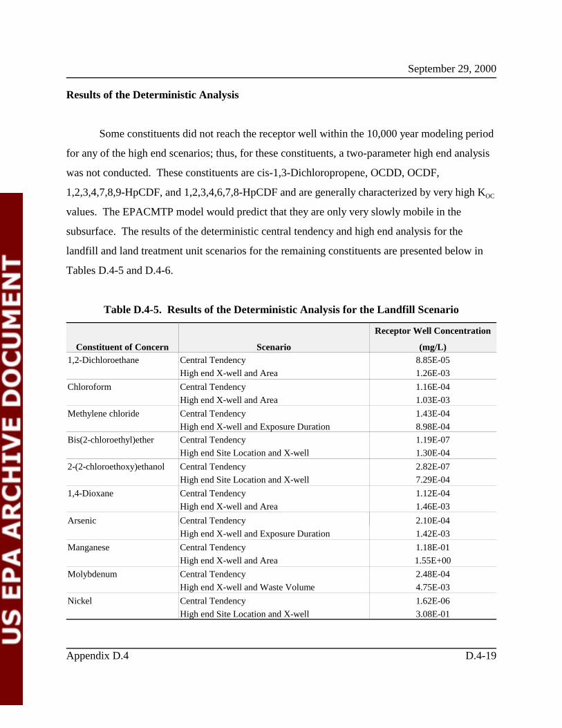
September 29, 2000

Appendix D.4 D.4-19

Results of the Deterministic Analysis

Some constituents did not reach the receptor well within the 10,000 year modeling period

for any of the high end scenarios; thus, for these constituents, a two-parameter high end analysis

was not conducted. These constituents are cis-1,3-Dichloropropene, OCDD, OCDF,

1,2,3,4,7,8,9-HpCDF, and 1,2,3,4,6,7,8-HpCDF and are generally characterized by very high KOC

values. The EPACMTP model would predict that they are only very slowly mobile in the

subsurface. The results of the deterministic central tendency and high end analysis for the

landfill and land treatment unit scenarios for the remaining constituents are presented below in

Tables D.4-5 and D.4-6.

Table D.4-5. Results of the Deterministic Analysis for the Landfill Scenario

Constituent of Concern Scenario

Receptor Well Concentration

(mg/L)1,2-Dichloroethane Central Tendency 8.85E-05

High end X-well and Area 1.26E-03

Chloroform Central Tendency 1.16E-04


Methylene chloride Central Tendency 1.43E-04

High end X-well and Exposure Duration 8.98E-04

Bis(2-chloroethyl)ether Central Tendency 1.19E-07

High end Site Location and X-well 1.30E-04

2-(2-chloroethoxy)ethanol Central Tendency 2.82E-07


1,4-Dioxane Central Tendency 1.12E-04


Arsenic Central Tendency 2.10E-04


Manganese Central Tendency 1.18E-01

High end X-well and Area 1.55E+00

Molybdenum Central Tendency 2.48E-04

High end X-well and Waste Volume 4.75E-03

Nickel Central Tendency 1.62E-06


September 29, 2000

Appendix D.4 D.4-20

Table D.4-6. Results of the Deterministic Analysis for the Land Treatment Unit Scenario

Constituent of Concern Scenario

Receptor Well

Concentration (mg/L)

Arsenic Central Tendency 1.88E-04

High end Leachate Concentration and Exposure Duration 5.00E-04

Bis(2-chloroethyl)ether Central Tendency 4.45E-06


2-(2-chloroethoxy)ethanol Central Tendency 1.08E-05


1,4-Dioxane Central Tendency 2.84E-05


Probabilistic Modeling For The Chlorinated Aliphatics Listing Determination

The purpose of the groundwater pathway Monte Carlo analysis is to provide a

probabilistic estimate of risk given the uncertainty and variability in groundwater pathway

parameters. The Monte Carlo analysis also provides an estimate of where in the distribution of

risk the results of the deterministic analysis fall. For this analysis, the output of the groundwater

fate and transport model is a probability distribution of receptor well concentrations. The Monte

Carlo analysis was only conducted for constituents which showed significant (for example,

greater than 1x10-6) risk in the high end deterministic analysis. For both the landfill and land

treatment unit scenarios, arsenic was the only constituent for which the Monte Carlo modeling

was performed.

Appendix F.1 provides a complete description of the EPACMTP site-based methodology,

the data sources for probability distributions of input parameters, and a detailed discussion of

how the source partitioning model and EPACMTP were linked in the Monte Carlo analysis. The

groundwater concentrations predicted in the Monte Carlo analysis are presented in Appendix H.

September 29, 2000

Appendix D.4 D.4-21

References

Allison, J.D., D.S. Brown, and K.H. Novo-Gradic, 1991. MINTEQA2/PRODEFA2,A ChemicalAssessment Model for Environmental Systems: Version 4.0 User’s Manual. EPA/600/3-91/021. U.S. EPA, Athens, GA.

Kollig, H.P. (ed). 1993.Environmental Fate Constants for Organic Constituents UnderConsideration for EPA’s Hazardous Waste Identification Projects.EPA/600/R-93/132.Environmental Research Laboratory, Office of Research and Development, Athens, GA.

Kool, J.B., P.S. Huyakorn, E.A. Sudicky, and Z.A. Saleem, 1994. A composite modelingapproach for subsurface transport of degrading contaminants from land disposal sites.Journal of Contaminant Hydrology, 17:69-90.

Loux, N. T., C. R. Chafin, and S. M. Hassan, 1990.Statistics of Aquifer Material Properties andEmpirical pH-dependent Partitioning Relationships for As (III), As (V), Ba(II), Cd(II),Cr(VI), Cu(II), Hg(II), Ni(II), Pb(II), Sb(V), Se(IV), Tl(I), and Zn(II). Office of Researchand Development, U.S. Environmental Protection Agency, Athens GA.

U.S. EPA (U.S. Environmental Protection Agency). 1996a. EPA'sComposite Model forLeachate Migration with Transformation Products (EPACMTP) Background Document.Office of Solid Waste, Washington, DC.

U.S. EPA (U.S. Environmental Protection Agency), 1996b. EPA'sComposite Model forLeachate Migration with Transformation Products (EPACMTP) Background Documentfor the Finite Source Methodology. Office of Solid Waste, Washington, DC.

U.S. EPA (U.S. Environmental Protection Agency), 1996c. EPA'sComposite Model forLeachate Migration with Transformation Products (EPACMTP) Background Documentfor Metals. Office of Solid Waste, Washington, DC.

U.S. EPA (U.S. Environmental Protection Agency), 1997a. EPA'sComposite Model forLeachate Migration with Transformation Products (EPACMTP) User's Guide. Office ofSolid Waste, Washington, DC.

U.S. EPA, 1997b. Analysis of Subtitle D Waste Management Units Databases used inGroundwater Pathway Analysis of HWIR - Draft. Office of Solid Waste. September,1997.

U.S. EPA, 1997c.Exposure Factors Handbook. Volume III: Activity Factors. EPA/600/P-95/002Fc. Office of Research and Development, Washington, D.C., 20460.

Appendix D.5

Surface Water Model

September 29, 2000

Appendix D.5 D.5-1

Appendix D.5

Surface Water Model

Introduction

The framework for estimating surface water impacts from the management of chlorinated

aliphatics wastes is based on the methodology presented inAddendum to Methodology for

Assessing Health Risks Associated with Indirect Exposure to Combustor Emissions(U.S. EPA,

1993), henceforth referred to as the Addendum. The model estimates water column and bed

sediment concentrations. Fish tissue concentrations are estimated from water column or

sediment concentrations using bioconcentration factors (BCFs), bioaccumulation factors (BAFs),

or biota-sediment accumulation factors (BSAFs).

Water column concentrations include dissolved, sorbed to suspended sediments, and total

concentration (sorbed plus dissolved). The model accounts for five routes of contaminant entry

into the waterbody: (1) contaminant sorbed to eroding soils, (2) contaminant dissolved in runoff,

(3) particle-bound contaminant deposition, (4) wet deposition of vapor phase contaminant, and

(5) direct diffusion of vapor phase contaminants. In addition, the model will accept input from

the groundwater model on contaminated groundwater that enters the waterbody through the

subsurface. The model also accounts for processes that remove contaminants. These include:

volatilization of dissolved phase contaminants from the water column and contaminant removal

September 29, 2000

Appendix D.5 D.5-2

via burial. The impact to the waterbody is assumed to be uniform, which is more realistic for

smaller waterbodies than for larger ones. Key assumptions in the model include the following:

ÿ Soil concentrations within the depositional area are uniform

ÿ Concentrations within the surface soils, sediments, suspended solids, and water can

be described by partition coefficients

ÿ At equilibrium, gaseous diffusion into the water equals volatilization from the water

ÿ Equilibrium is maintained between contaminants within the water column and

contaminants in sediment

ÿ Rate of contaminant burial in bed sediments is estimated as a function of the sediment

deposition rate.

The scenario modeled for to predict fisher risks simulates contaminant loadings to a reach

order 3 stream located at either a high end (102 m) or central tendency distance (430 m for the

LTU; 300 m for other units) from the source to the stream.

Waterbody/Watershed Characterization

The parameters contained in this section characterize the surface waterbody (a stream)

simulated by the model. The waterbody characterization parameters are another example of a set

of parameters that are interdependent; therefore, they are set and varied as a group.

Van der Leeden et al. (1990) ranked over 2 million streams located throughout the United

States according to their stream order. A first-order stream has no tributary channels; a second-

September 29, 2000

Appendix D.5 D.5-3

order stream forms when two first-order streams converge, and so on through stream order 10.

Each successive stream order is characterized by a larger flow volume. For each stream order,

van der Leeden presented typical values for flow, waterbody area, watershed area, depth, and

various other parameters. A third order stream reach was chosen as the waterbody for the

modeling simulations in this analysis and was characterized using van der Leeden's typical values

for the third order stream reach. Van der Leeden's data on stream reaches are reproduced in

Table D.5-1.

Stream orders 1 and 2 are typically too small to support the fish consumption assumed

under the fisher scenario and, therefore, were eliminated from consideration. Of the stream

orders sufficiently large to support aquatic life for fishing (stream orders 3 through 10), we

selected stream order 3 to create an exposure scenario that was protective of different types of

fishable waterbodies and, at the same time, representative of streams on a national basis. As

shown in Table D.5.1, reach order 3 streams are more prevalent in terms of sheer number than all

other fishable streams and rivers combined; thus, the reach order 3 streams would be expected to

be accessible to fishers in most areas of the country. In addition, the total length for reach order

3 streams is within 10% of all the other fishable streams and rivers combined. Lastly, the

conceptual framework for this simulation uses a single point estimate for air concentration and

deposition rate. As an approximation, use of a single value is reasonable for a small stream such

as that described under reach order 3. As noted in the Technical Background Document, this

scenario was developed to be protective of all recreational and subsistence fisher scenarios.

However, using a single point estimate for a reach order 5 stream was not considered to be a

reasonable approach to estimating fish concentrations, and would have resulted in a significant

overestimate of the fisher risks. Based on this information, a reach order 3 stream was used as

the fishable waterbody in the risk modeling simulations for the fisher scenario.

Table D.5-2 summarizes the stream data used to characterize the reach order 3 stream.

These values are converted to metric units, as needed by the model. Watershed area (called

September 29, 2000

Appendix D.5 D.5-4

drainage area by van der Leeden), flow, depth, and velocity were taken directly from van der

Leeden. Waterbody area was calculated from average length and width. Flow-independent

mixing volume was calculated from average length, width, and depth, as suggested in the

Addendum.

Table D.5-1. Summary of U.S. Stream Data

Stream

order

Number

of

streams

Total

length

(mi)

Average

length

(mi)

Drainage

area

(mi2)

Surface

area

(mi2)

Mean

flow

(ft 3/s)

Mean

width

(ft)

Mean

depth

(ft)

Mean

velocity

(ft/s)

1 1,570,000 1,570,000 1.0 1.0 1,200 0.65 4 0.15 1.0

2 350,000 810,000 2.1 4.7 1,500 3.1 10 0.29 1.3

3 80,000 420,000 5.3 23 1,400 15 18 0.58 1.5

4 18,000 220,000 12 109 1,500 71 37 1.1 1.8

5 4,200 116,000 28 518 1,600 340 75 2.2 2.3

6 950 61,000 64 2,500 1,800 1,600 160 4.1 2.7

7 200 30,000 147 12,000 1,800 7,600 320 8.0 3.3

8 41 14,000 338 56,000 1,700 36,000 650 15 3.9

9 8 6,200 777 260,000 1,500 171,000 1,300 29 5.6

10 1 1,800 1,800 1,250,000 1,000 810,000 2,800 55 5.9

Source: Van der Leeden et al. (1990).

September 29, 2000

Appendix D.5 D.5-5

Table D.5-2. Characterization of Reach Order 3 Stream

Parameter Stream Order 3

Watershed area 6e+7 m2

Flow

1.3e+7 m3/yr

(1.3e+10 L/yr)

Velocity 0.5 m/s

Depth (waterbody) 0.18 m

Width 5.5 m

Length 8,500 m

Waterbody area

(length × width) 4.6e+4 m2

Flow-independent mixing volume (length × width × depth)

8.3e+3 m3

(8.3e+6 L)

Depth (bed sediment) 0.03 m

Depth (water column) 0.15 m

The surface water model requires three different depth measurements as inputs: depth of

the water column, depth of bed sediment, and total waterbody depth (which is the sum of the

water column and sediment depths). The depth from van der Leeden was for total waterbody

depth. The Addendum suggests a typical bed sediment depth of 0.03 m; this was used, and the

water column depth calculated as the difference between the total waterbody depth from van der

Leeden and the bed sediment depth of 0.03 m.

September 29, 2000

Appendix D.5 D.5-6

Other Surface Water Parameters

Total Suspended Solids

The Addendum suggests that total suspended solids (TSS) can range from 1 to 100 mg/L

and suggests a “typical” value of 10 mg/L for streams and rivers. However, given the depth of

the stream and flow rate, we might expect to have a higher value for TSS than the “typical” value

recommended for streams and rivers of all sizes (e.g., small, shallow streams will have less

settling of suspended solids because of turbulence). The Addendum suggests that 80 mg/L is a

cutoff value for protection of aquatic life and, therefore, this value was selected for the reach

order 3 stream. It should be noted that varying the TSS concentration has little impact on the

modeling results on metals and hydrophilic organic constituents (i.e., organic chemicals with the

log Kow value below 4.0). However, for highly hydrophobic constituents such as dioxins,

decreasing the TSS to 10 mg/L from 80 mg/L results in less than a two-fold increase in risks

from ingestion fish, with all other parameters set to the same value. Thus, the model is only

moderately sensitive to this parameter, and the default TSS value of 80 mg/L is considered a

minor source of uncertainty.

Bed Sediment Concentration

The bed sediment concentration term is analogous to the bulk density for soil in that it

describes the concentration of solids in terms of a mass per unit volume. The Addendum notes

that bed sediment concentration should range from 0.5 to 1.5 kg/L and that a reasonable value for

most applications is 1 kg/L. Given the narrow range for this parameter, the recommendation in

the Addendum was adopted.

September 29, 2000

Appendix D.5 D.5-7

ÿbsÿ 1�BS�s

(D.5-(26))

Bed Sediment Porosity

The bed sediment porosity describes the volume of water per volume of benthic space.

Bed sediment porosity is calculated from bed sediment concentration and sediment density as

follows (Addendum):

where

ÿbs = bed sediment porosity (L/L)

BS = bed sediment concentration = 1 kg/L = 1,000,000 mg/L

�s = sediment density = 2.65 kg/L (a standard value for mineral materials).

This results in a value of 0.6 that was used in the modeling simulations.

Gas-Phase Transfer Coefficient

The gas-phase transfer coefficient is used to estimate volatile losses from the waterbody.

Volatile losses are calculated using a two-layer resistance model that incorporates a gas-phase

transfer coefficient and a liquid-phase transfer coefficient. Both transfer coefficients are

controlled by flow-induced turbulence in flowing systems. The liquid-phase transfer coefficient

is calculated based on chemical-specific properties as specified in the Addendum. The

Addendum recommends a single value for the gas-phase transfer coefficient for flowing systems

of 36,500 m/yr.

September 29, 2000

Appendix D.5 D.5-8

There is some uncertainty around setting this parameter to a single value that is not

chemical specific. It is reasonable to assume that chemical properties affecting volatility would

have some effect on this value, although it is not known how large such an effect would be. The

Addendum does give an equation (using chemical-specific properties) for calculating this

parameter for stagnant systems, such as lakes or ponds. However, the transfer coefficients for

stagnant systems are dominated by wind-induced turbulence rather than flow-induced turbulence;

therefore, this equation is not applicable to flowing systems such as are modeled here and is not

used.

Fraction Organic Carbon in Bottom Sediment

The fraction organic carbon in bottom sediment is derived from the fraction organic

carbon in watershed soils. This value is “site-specific” and the same value is used for the

waterbody as is used for the nonwaterbody soils.

Waterbody Temperature

An average surface waterbody temperature of 298 K (25�C) was considered a "common

assumption for water temperature" in the Addendum. Although this value is somewhat high, the

results are insensitive to this parameter, and reasonable lower values should have no effect on the

results. This temperature was used to estimate gaseous diffusion loads into the surface

waterbody.

Fish Concentrations

The chemical constituents in the water column exist in both the freely dissolved phase

and sorbed to suspended solids or dissolved organic carbon. For all constituents, the dissolved

fraction is the most bioavailable form and is used to predict the fish concentrations whenever

September 29, 2000

Appendix D.5 D.5-9

biological uptake data (i.e., BCFs, BAFs, or BSAFs) are available for the dissolved phase of the

constituent. In some cases (e.g., for metals), the biological uptake data are taken from studies

that considered only the total concentration of the chemical, that is, the dissolved phaseandthe

sorbed phase. For these constituents, the fish concentrations are predicted using a total chemical

concentration rather than the freely dissolved concentration. The estimated surface water

concentrations (see Appendix E for equations) are used to predict the concentration of

contaminants in fish by applying constituent-specific biological uptake factors.

One of three types of biological uptake factors is used in the calculation of fish tissue

concentrations: bioconcentration factors (BCFs), bioaccumulation factors (BAFs), and biota-

sediment accumulation factors (BSAFs). Bioconcentration is defined as the net uptake of a

chemical from an organism’s surrounding medium through direct contact (e.g., uptake by a fish

through the gill exchange) but excluding ingestion of contaminated plants or prey.

Bioaccumulation is defined as the net uptake of a chemical from the environment from all

pathways (including direct contact and ingestion of contaminated plants or prey). It is important

to recognize that the distinction between BCF and BAF has both practical and technical

implications. The route of exposure assumed for BCFs is direct contact, and BCF values are

typically generated from controlled laboratory studies where fish are exposed to the chemical

only through water. For organic chemicals with log Kow values below ~4.0 (referred to here as

hydrophilic organics), the BCF provides a reasonable estimate of the concentration expected to

be found in fish under field conditions. However, for more hydrophobic organic chemicals (log

Kow >> 4.0), uptake via the food chain will be an increasingly important source of exposure, and

using a BCF will tend to underestimate the concentration in fish tissue. Therefore, for

hydrophobic organic chemicals, and other chemicals shown to bioaccumulate (e.g., mercury), a

BAF is the preferred factor to use for estimating fish tissue concentrations. BAFs are typically

generated from field studies or estimated from models.

September 29, 2000

Appendix D.5 D.5-10

Cfishÿ Cw x BAF (D.5-(27))

Cfishÿ Cw x BCF (D.5-(28))

In addition to the distinction between BCFs and BAFs, it is important to recognize the

difference between dissolved water concentrations versus total water concentrations. As noted

above, the surface water concentrations for hydrophilic organics are typically regarded as freely

dissolved, although a small fraction will be sorbed to dissolved organic carbon (DOC) and larger

organic particles. For hydrophobic organic chemicals, a significant fraction of the total water

concentration is sorbed to DOC and particles. Unless filtration methods were used to analyze

the freely dissolved concentration in the water, the reported biological uptake factors may reflect

total rather than the dissolved water concentration. Thus, it is important to select the appropriate

water concentration (freely dissolved or total) depending on the biological uptake factor that is

available. For hydrophilic organics, we generally used the freely dissolved water concentration

because the study-generated BCFs and BAFs (as well as the empirical algorithms) reflect the

dissolved concentration in surface water. In contrast, we typically use the total concentrations for

metals and hydrophobic organics because the BCFs and BAFs often are based on total rather than

freely dissolved water concentrations.

The following equations are used to estimate fish tissue concentrations for constituents of

concern other than dioxins:

or

where

Cfish = fish concentration (mg/kg)

Cw = water concentration - dissolved or total (mg/L)

BAF = bioaccumulation factor - dissolved or total (L/kg)

BCF = bioconcentration factor - dissolved or total (L/kg).

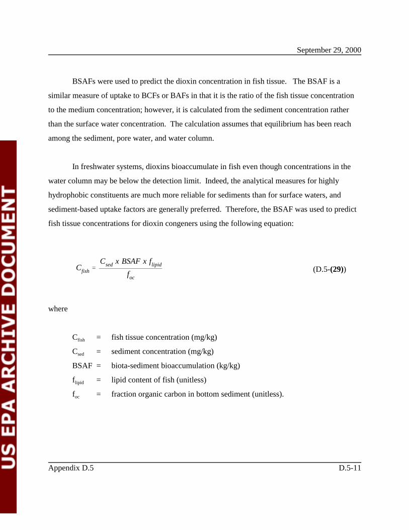
September 29, 2000

Appendix D.5 D.5-11

CfishÿCsed x BSAF x flipid

foc

(D.5-(29))

BSAFs were used to predict the dioxin concentration in fish tissue. The BSAF is a

similar measure of uptake to BCFs or BAFs in that it is the ratio of the fish tissue concentration

to the medium concentration; however, it is calculated from the sediment concentration rather

than the surface water concentration. The calculation assumes that equilibrium has been reach

among the sediment, pore water, and water column.

In freshwater systems, dioxins bioaccumulate in fish even though concentrations in the

water column may be below the detection limit. Indeed, the analytical measures for highly

hydrophobic constituents are much more reliable for sediments than for surface waters, and

sediment-based uptake factors are generally preferred. Therefore, the BSAF was used to predict

fish tissue concentrations for dioxin congeners using the following equation:

where

Cfish = fish tissue concentration (mg/kg)

Csed = sediment concentration (mg/kg)

BSAF = biota-sediment bioaccumulation (kg/kg)

flipid = lipid content of fish (unitless)

foc = fraction organic carbon in bottom sediment (unitless).

September 29, 2000

Appendix D.5 D.5-12

References

U.S. EPA (Environmental Protection Agency). 1993.Addendum to Methodology for Assessing

Health Risks Associated with Indirect Exposure to Comubstor Emissions. EPA/600/AP-

93003. Office of Health and Environmental Assessment, Washington, DC.

Van der Leeden, F., F.L. Troise, and D.K. Todd. 1990.The Water Encyclopedia. 2nd ed.

Chelsea, MI: Lewis Publishers.

Appendix F.1

Monte Carlo Fate and Transport Modeling

September 29, 2000

Appendix F.1 F.1-3

Appendix F.1

Monte Carlo Fate and Transport Modeling

Introduction

The probabilistic analysis addresses only constituents and pathways that had an excess

lifetime cancer risk of 10-6 or greater or a hazard quotient of 1 or greater. Spreadsheet models,

computer programs, and Crystal Ball™ version 4.0d were used to run the Monte Carlo analysis.

This document describes how the common input parameters, their distributions, and the transfer

of input-output data were handled.

Eight waste quantities were used in the probabilistic assessment for wastewaters managed

in tanks (Table 2-4) and nine wastewater sludge quantities were used for the landfills (Table 2-6).

Only one waste quantity was used for the land treatment unit (LTU) because only one facility

uses an LTU. Waste quantity and facility location were independent variables in the risk

assessment.

For the deterministic analysis, an average waste concentration and a maximum

concentration were used to represent the central tendency and high-end concentrations,

respectively. For the Monte Carlo analysis, waste concentrations were determined by selecting

one of the available samples at random. Each sample (see Tables 2-1, 2-2, and 2-3) had an equal

probability of being selected. Constituents of concern (COCs) for the LTU included dioxins

September 29, 2000

Appendix F.1 F.1-4

(nongroundwater pathways), arsenic (nongroundwater and groundwater pathways), and

chromium (direct inhalation). Arsenic (groundwater ingestion) was the only COC for the

landfill. Dioxins were the only COCs for wastewaters.

The key distinction between deterministic and Monte Carlo analyses is that for the

deterministic analysis, each input parameter is set at either a central tendency or high-end value

with a maximum of two parameters set at the high-end value at any time. For the Monte Carlo

analysis on the other hand, probability density functions (PDFs) are developed that describe the

full range of values for the various input parameters. The result from the Monte Carlo analysis is

a probability distribution of exposures and risk, rather than a single value. PDFs for input

parameters used to model constituents released from EDC/VCM wastewater sludges managed in

a landfill are shown in Figure F.1-1 (unsaturated zone), Figure F.1-2 (saturated zone), and Figure

F.1-3 (source specific parameters). Unsaturated zone, saturated zone, and source specific input

PDFs used to model the LTU are shown in Figures F.1-4, Figure F.1-5, and F.1-6, respectively.

PDFs are not shown for waste concentration (Tables 2-1 to 2-3), waste quantities (Tables 2-4 and

2-6), location (Tables 2-5 and 2-6), or distance to receptor (50, 75, 100, 200, 300, 500, and 1000

m) because values were selected with equal probability from a limited number of available or

selected values rather than a continuous distribution. The various input parameters used in the

Monte Carlo analysis are described in Appendix K.

For the non-groundwater pathway analyses, fate and transport modeling and exposure

modeling were linked together and are discussed in more detail in Appendix F.2. For

groundwater pathways, the fate and transport models are separate from the exposure modeling.

A PDF for groundwater concentrations at the groundwater exposure point (receptor well) is

generated from the EPACMTP model. PDFs for groundwater concentrations generated for the

landfill and LTU are shown in Figures F.1a and F.1-7b, respectively. The groundwater

concentration PDF is then combined with exposure parameters (discussed in Appendix F.2) to

generate a distribution of risk for each receptor. Therefore, in order to conduct a probabilistic

September 29, 2000

Appendix F.1 F.1-5

risk analysis for groundwater exposure pathways, it was necessary to link output from the

partitioning model with the groundwater model. The following sections describe the Monte

Carlo methodologies used for groundwater fate and transport modeling.

Groundwater Pathway Monte Carlo Modeling

Detailed background for the Monte Carlo option in EPACMTP is provided in U.S. EPA

1997a and b. In order to run EPACMTP in Monte Carlo mode, a probability distribution must be

provided for each input parameter (except constant or derived parameters). The Monte Carlo

methodology is then performed as follows. The model input data are read first, followed by

generation of a sequence of random numbers. This sequence of random numbers is then used to

generate the pseudo-random values of the uncertain input variable(s) (drawn from the known

distribution and within the range of any imposed bounds). The derived parameter values are then

calculated. Following this, the contaminant fate and transport simulation is performed. The

result is given in terms of the predicted contaminant concentrations in a downgradient receptor

well. The generation of random parameter values and the fate and transport simulation is then

repeated as many times as desired to generate a set of resulting receptor well concentrations.

This model output is then statistically analyzed to yield the cumulative probability distribution of

groundwater concentrations. A key aspect of the Monte Carlo analysis is the preservation of

correlations between various model parameters, e.g. between waste site location and infiltration

and recharge rate, and between location and hydrogeologic parameters. In order to maintain these

dependencies in the analysis, a regional site-based modeling database has been developed (U.S.

EPA, 1997a,b), which associates any waste unit location in the continental United States with

one of 13 hydrogeologic regions and one of 97 climatic regions and provides modeling parameter

values for each of these hydrogeological and climate regions. This database utilizes the U.S.

Geological Survey (USGS) inventory of the groundwater resources of each state (Heath, 1984),

and the Hydrogeologic Database for Modeling (HGDB) (API, 1989; U.S. EPA, 1997a and

September 29, 2000

Appendix F.1 F.1-6

1997b), developed from a survey of hydrogeologic parameters for actual hazardous waste sites in

the United States.

Groundwater Pathway Monte Carlo Modeling for Land Treatment Units

Since there is only one Chlorinated Aliphatics facility that land applies their EDC/VCM

sludge, only one waste unit location and waste volume were used for the Monte Carlo analysis.

In the present analysis, the calculation of leachate concentrations for the land treatment

unit, and calculation of landfill volatilization losses, respectively (see Appendix D.1), were

performed outside of the EPACMTP model. In order to ensure conservation of mass between the

source partitioning model and EPACMTP groundwater pathway model, the models must be fully

synchronized so that the same values for common input parameters are used in each individual

Monte Carlo realization. In the Monte Carlo modeling, the output from the source partitioning

model which is used as input for the groundwater modeling thus includes values for parameters

such as waste unit area, and infiltration rate.

To implement the required Monte Carlo linkage between the land treatment unit

partitioning model and EPACMTP, the data output routines of RTI’s partitioning model were

modified to generate output files that provide not only the leachate concentrations for each

realization, but also the corresponding input values of common modeling parameters. For the

Chlorinated Aliphatics analysis, these parameters are

ÿ Waste Management Unit Area

ÿ Infiltration Rate

ÿ Site Location (in terms of hydrogeologic and climatic region)

ÿ Maximum 9-year Average Leachate Concentration.

September 29, 2000

Appendix F.1 F.1-7

For the land treatment unit scenario, the source partitioning model was used to calculate

the leachate concentration of arsenic (the only constituent modeled in the Monte Carlo analysis)

infiltrating to the subsurface. This source model was run in Monte Carlo mode for 1,000

realizations to generate a probability distribution of leachate concentrations, creating a land

treatment unit source data file of 1,000 records. This data file was then used as input to the

EPACMTP groundwater fate and transport model. For this purpose, the EPACMTP data input

routines were modified to read in the values of Monte Carlo parameters that are common to both

models from this data file rather than generate these parameter values internally. For each

realization of the subsequent groundwater pathway Monte Carlo analysis, EPACMTP picked a

random record (with replacement) from the appropriate source file and read in the values of the

common input parameters in that record. The hydrogeologic region and climate region indices

that are specific to the LTU waste unit site were employed to choose random values for other

saturated and unsaturated zone parameters appropriate to the waste unit location associated with

the chosen record. For each of the 2,000 EPACMTP Monte Carlo realizations, the receptor well

concentration of interest, e.g., maximum 9-year average concentration, was then calculated and

saved to an output file. At the conclusion of the modeling, a PDF for the maximum 9-year

average receptor well concentration was constructed.

For the landfill Monte Carlo modeling, a database of Chlorinated Aliphatics facility

locations was created. Each facility location was assigned a hydrogeologic region number, a

climate region number, a groundwater temperature, and an infiltration rate, from the OSW

nationwide groundwater modeling database (U.S. EPA, 1997a,b). The landfill source

partitioning was applied to generate a distribution of the mass volatilized during the active life of

the landfill. The output of this model was a source data file of 1,000 records; each record

contained the following data: landfill area, landfill depth, infiltration rate, waste concentration,

initial leachate (TCLP) concentration, groundwater temperature, climate region number, and

hydrogeologic region number. The leachate concentrations were chosen from TCLP sampling

data.

September 29, 2000

Appendix F.1 F.1-8

To implement the required Monte Carlo linkage between the landfill volatilization model

and EPACMTP, the data output routines of the volatilization model were modified in a manner

similar to the land treatment unit partitioning model. That is, the output files provide not only

the leachate concentrations for each realization, but also the corresponding input values of

common modeling parameters.

For the first realization of the volatilization model, one value was chosen for each model

input and the source partitioning equations were then used to generate the amount of mass

volatilized. This mass volatilized and the input values for all common modeling parameters

were saved as one record of an ASCII data file. This process was then repeated 1,000 times,

producing an output data file containing 1,000 records. The waste concentration was then

corrected for the volatilization mass loss and added to the data file. This data file was then used

as input to the EPACMTP groundwater fate and transport model.

For each realization of the subsequent groundwater pathway Monte Carlo analysis,

EPACMTP picked a random record (with replacement) from the appropriate source file; the

model then read in the values of the common input parameters in that record. The hydrogeologic

region and climate region indices that are specific to each waste unit site were then employed to

choose random values for other saturated and unsaturated zone parameters appropriate to the

waste unit location associated with the chosen record. For each of the 2,000 EPACMTP Monte

Carlo realizations, the receptor well concentration of interest, e.g., maximum 9-year average

concentration, was then calculated and saved to an output file. At the conclusion of the

modeling, a PDF for the maximum 9-year average receptor well concentration was constructed.

September 29, 2000

Appendix F.1 F.1-9

0

50

100

150

200

250

300

Saturate d Conductivity (m /yr )

Fre

qu

en

cy

0%

10%

20%

30%

40%

50%

60%

70%

80%

90%

100%

Cu

mu

lati

ve%

0

50

100

150

200

250

300

350

400

450

500

Uns aturate d Zone Thick ne s s (m )F

req

ue

ncy

0%

10%

20%

30%

40%

50%

60%

70%

80%

90%

100%

Cu

mu

lati

ve%

0

100

200

300

400

500

600

700

800

M ois ture Re te ntion, Alpha (1/m )

Fre

qu

en

cy

0%

10%

20%

30%

40%

50%

60%

70%

80%

90%

100%

Cu

mu

lati

ve%

0

100

200

300

400

500

600

M ois ture Re te ntion, Be ta (un it le s s )

Fre

qu

en

cy

0%

10%

20%

30%

40%

50%

60%

70%

80%

90%

100%

Cu

mu

lati

ve%

0

50

100

150

200

250

300

350

400

450

500

Re s idual Wate r Conte nt (unit le s s )

Fre

qu

en

cy

0%

10%

20%

30%

40%

50%

60%

70%

80%

90%

100%

Cu

mu

lati

ve%

0

200

400

600

800

1000

1200

Saturate d Wate r Conte nt (un itle s s )

Fre

qu

en

cy

0%

10%

20%

30%

40%

50%

60%

70%

80%

90%

100%

Cu

mu

lati

ve%

0

200

400

600

800

1000

1200

1400

1600

1800

Soil Bulk De ns ity (g/cm 3)

Fre

qu

en

cy

0%

10%

20%

30%

40%

50%

60%

70%

80%

90%

100%

Cu

mu

lati

ve%

0

100

200

300

400

500

600

700

Pe rce nt Organic M atte r (unitle s s )

Fre

qu

en

cy

0%

10%

20%

30%

40%

50%

60%

70%

80%

90%

100%

Cu

mu

lati

ve%

Figure F.1-1. Monte Carlo Input Parameters, Landfill - Unsaturated Zone

September 29, 2000

Appendix F.1 F.1-10

0

50

100

150

200

250

300

350

400

450

500

Par ticle Diam e te r (cm )

Fre

qu

en

cy

0%

10%

20%

30%

40%

50%

60%

70%

80%

90%

100%

Cu

mu

lati

ve%

0

100

200

300

400

500

600

700

Aquife r Thick ne s s (m )

Fre

qu

en

cy

0%

10%

20%

30%

40%

50%

60%

70%

80%

90%

100%

Cu

mu

lati

ve%

0

50

100

150

200

250

300

350

400

450

500

Hydraulic Gradie nt (m /m )F

req

ue

ncy

0%

10%

20%

30%

40%

50%

60%

70%

80%

90%

100%

Cu

mu

lati

ve%

0

100

200

300

400

500

600

700

800

Longitud inal Dis pe rs ivity (m )

Fre

qu

en

cy

0%

10%

20%

30%

40%

50%

60%

70%

80%

90%

100%

Cu

mu

lati

ve%

0

100

200

300

400

500

600

Trans ve rs e Dis pe rs ivity (m )

Fre

qu

en

cy

0%

10%

20%

30%

40%

50%

60%

70%

80%

90%

100%

Cu

mu

lati

ve%

0

50

100

150

200

250

Poros ity (un it le s s )

Fre

qu

en

cy

0%

10%

20%

30%

40%

50%

60%

70%

80%

90%

100%

Cu

mu

lati

ve%

050

100150

200250

300350

400450

500

Hydraulic Conductivity (m /yr )

Fre

qu

en

cy

0%10%

20%30%

40%50%

60%70%

80%90%

100%

Cu

mu

lati

ve%

0

100

200

300

400

500

600

Saturate d Bulk De ns ity (g/cm 3)

Fre

qu

en

cy

0%

10%

20%

30%

40%

50%

60%

70%

80%

90%

100%

Cu

mu

lati

ve%

Figure F.1-2. Monte Carlo Input Parameters, Landfill -Saturated Zone

September 29, 2000

Appendix F.1 F.1-11

0

50

100

150

200

250

300

350

V e r tical Dis pe rs ivity (m )

Fre

qu

en

cy

0%

10%

20%

30%

40%

50%

60%

70%

80%

90%

100%

Cu

mu

lati

ve%

0

50

100

150

200

250

300

350

X-Dis tance to Re ce ptor We ll (m )

Fre

qu

en

cy

0%

10%

20%

30%

40%

50%

60%

70%

80%

90%

100%

Cu

mu

lati

ve%

0

50

100

150

200

250

300

350

Se e page V e locity (m /yr )

Fre

qu

en

cy

0%

10%

20%

30%

40%

50%

60%

70%

80%

90%

100%

Cu

mu

lati

ve%

0

50

100

150

200

250

300

350

400

450

Aquife r pH (s tandard units )

Fre

qu

en

cy

0%

10%

20%

30%

40%

50%

60%

70%

80%

90%

100%

Cu

mu

lati

ve%

0

100

200

300

400

500

600

Y-Dis tance to We ll (m )F

req

ue

ncy

0%

10%

20%

30%

40%

50%

60%

70%

80%

90%

100%

Cu

mu

lati

ve%

0

100

200

300

400

500

600

Fraction Organic Carbon (unit le s s )

Fre

qu

en

cy

0%

10%20%

30%

40%

50%60%

70%

80%90%

100%

Cu

mu

lati

ve%

0

50

100

150

200

250

300

350

Re ce ptor We ll De pth (m )

Fre

qu

en

cy

0%

10%

20%

30%

40%

50%

60%

70%

80%

90%

100%

Cu

mu

lati

ve%

Figure F.1-2. Continued

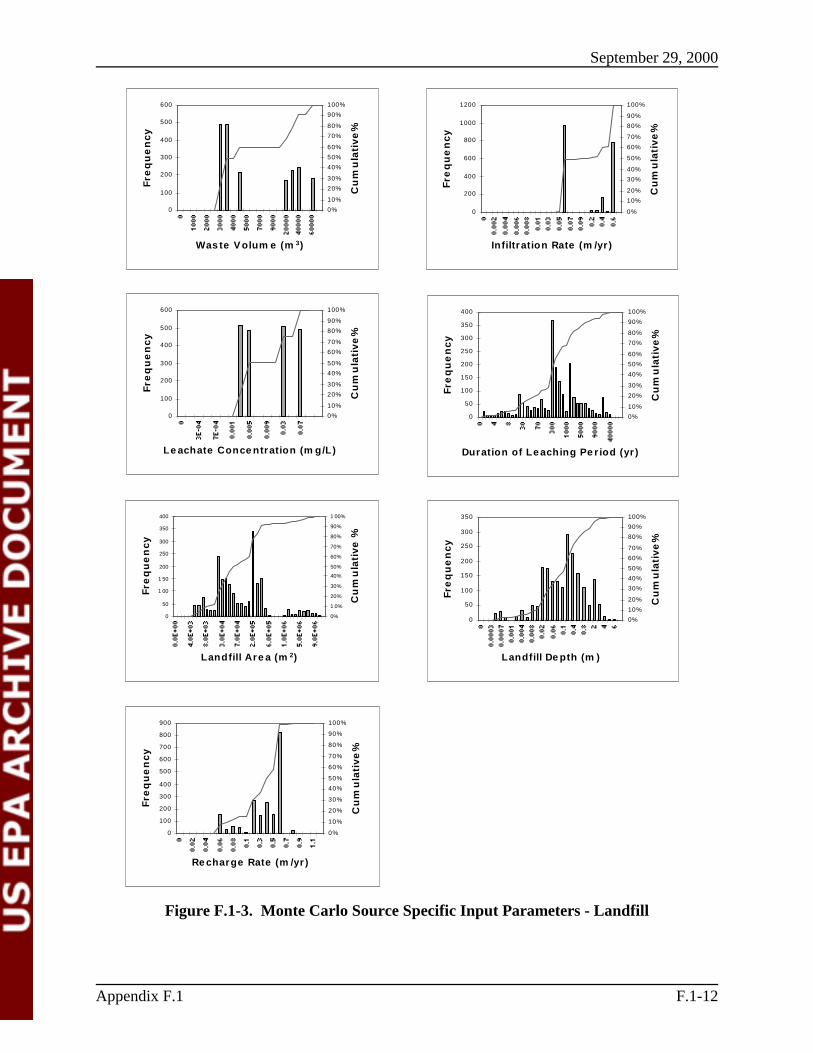
September 29, 2000

Appendix F.1 F.1-12

0

50

1 00

1 50

200

250

300

350

400

Landfill Are a (m 2)

Fre

qu

en

cy

0%

1 0%

20%

30%

40%

50%

60%

70%

80%

90%

1 00%

Cu

mu

lati

ve%

0

100

200

300

400

500

600

700

800

900

Re charge Rate (m /yr )

Fre

qu

en

cy

0%

10%

20%

30%

40%

50%

60%

70%

80%

90%

100%

Cu

mu

lati

ve%

0

200

400

600

800

1000

1200

In filtration Rate (m /yr )

Fre

qu

en

cy

0%

10%

20%

30%

40%

50%

60%

70%

80%

90%

100%

Cu

mu

lati

ve%

0

100

200

300

400

500

600

Le achate Conce ntration (m g/L)

Fre

qu

en

cy

0%

10%

20%

30%

40%

50%

60%

70%

80%

90%

100%

Cu

mu

lati

ve%

0

50

100

150

200

250

300

350

Landfill De pth (m )

Fre

qu

en

cy

0%

10%

20%

30%

40%

50%

60%

70%

80%

90%

100%

Cu

mu

lati

ve%

0

100

200

300

400

500

600

Was te V olum e (m 3)

Fre

qu

en

cy

0%

10%

20%

30%

40%

50%

60%

70%

80%

90%

100%

Cu

mu

lati

ve%

0

50

100

150

200

250

300

350

400

Duration of Le aching Pe r iod (yr )F

req

ue

ncy

0%

10%

20%

30%

40%

50%

60%

70%

80%

90%

100%

Cu

mu

lati

ve%

Figure F.1-3. Monte Carlo Source Specific Input Parameters - Landfill

September 29, 2000

Appendix F.1 F.1-13

0

50

100

150

200

250

300

Saturate d Conductivity (m /yr)

Fre

qu

en

cy

0%

10%

20%

30%

40%

50%

60%

70%

80%

90%

100%

Cu

mu

lati

ve%

0

100

200

300

400

500

600

700

800

M ois ture Re te ntion, A lpha (1/m )

Fre

qu

en

cy

0%

10%

20%

30%

40%

50%

60%

70%

80%

90%

100%

Cu

mu

lati

ve%

0

100

200

300

400

500

600

M ois ture Re te ntion, Be ta (un itle s s )

Fre

qu

en

cy

0%

10%

20%

30%

40%

50%

60%

70%

80%

90%

100%

Cu

mu

lati

ve%

0

50

100

150

200

250

300

350

400

450

Re s idual Wate r Conte nt (un itle s s )

Fre

qu

en

cy

0%

10%

20%

30%

40%

50%

60%

70%

80%

90%

100%

Cu

mu

lati

ve%

0

200

400

600

800

1000

1200

1400

Saturate d Wate r Conte nt (unit le s s )

Fre

qu

en

cy

0%

10%

20%

30%

40%

50%

60%

70%

80%

90%

100%

Cu

mu

lati

ve%

0

50

100

150

200

250

300

350

400

450

Uns aturate d Zone Thick ne s s (m )F

req

ue

ncy

0%

10%

20%

30%

40%

50%

60%

70%

80%

90%

100%

Cu

mu

lati

ve%

0

200

400

600

800

1000

1200

1400

1600

1800

2000

Uns aturate d Bulk De ns ity (g/cm 3)

Fre

qu

en

cy

0%

10%

20%

30%

40%

50%

60%

70%

80%

90%

100%

Cu

mu

lati

ve%

0

100

200

300

400

500

600

700

Pe rce nt Organic M atte r (un it le s s )

Fre

qu

en

cy

0%

10%

20%

30%

40%

50%

60%

70%

80%

90%

100%

Cu

mu

lati

ve%

Figure F.1-4. Monte Carlo Input Parameters, Land Treatment Unit - Unsaturated Zone

September 29, 2000

Appendix F.1 F.1-14

0

50

100

150

200

250

300

350

400

450

Par ticle Diam e te r (cm )

Fre

qu

en

cy

0%

10%

20%

30%

40%

50%

60%

70%

80%

90%

100%

Cu

mu

lati

ve%

0

100

200

300

400

500

600

Longitud inal Dis pe rs ivity (m )

Fre

qu

en

cy

0%

10%

20%

30%

40%

50%

60%

70%

80%

90%

100%

Cu

mu

lati

ve%

0

100

200

300

400

500

600

Trans ve rs e Dis pe rs ivity (m )

Fre

qu

en

cy

0%

10%

20%

30%

40%

50%

60%

70%

80%

90%

100%

Cu

mu

lati

ve%

0

50

100

150

200

250

300

350

400

450

Aquife r Thick ne s s (m )

Fre

qu

en

cy

0%

10%

20%

30%

40%

50%

60%

70%

80%

90%

100%

Cu

mu

lati

ve%

0

20

40

60

80

100

120

140

160

180

200

Poros ity (un it le s s )

Fre

qu

en

cy

0%

10%

20%

30%

40%

50%

60%

70%

80%

90%

100%

Cu

mu

lati

ve%

0

100

200

300

400

500

600

Saturate d Bulk De ns ity (g /cm 3)

Fre

qu

en

cy

0%

10%

20%

30%

40%

50%

60%

70%

80%

90%

100%

Cu

mu

lati

ve%

0

50

100

150

200

250

300

Hydraulic Conductivity (m /yr )

Fre

qu

en

cy

0%

10%

20%

30%

40%

50%

60%

70%

80%

90%

100%

Cu

mu

lati

ve%

0

50

100

150

200

250

300

350

Hydraulic Gradie nt (un itle s s )F

req

ue

ncy

0%

10%

20%

30%

40%

50%

60%

70%

80%

90%

100%

Cu

mu

lati

ve%

Figure F.1-5. Monte Carlo Input Parameters, Land Treatment Unit - Saturated Zone

September 29, 2000

Appendix F.1 F.1-15

0

50

100

150

200

250

300

350

400

450

Se e page V e locity (m /yr )

Fre

qu

en

cy

0%

10%

20%

30%

40%

50%

60%

70%

80%

90%

100%

Cu

mu

lati

ve%

0

50

100

150

200

250

300

350

X-Dis tance to Re ce ptor We ll (m )

Fre

qu

en

cy

0%

10%

20%

30%

40%

50%

60%

70%

80%

90%

100%

Cu

mu

lati

ve%

0

100

200

300

400

500

600

700

Y-Dis tance to Re ce ptor We ll (m )F

req

ue

ncy

0%

10%

20%

30%

40%

50%

60%

70%

80%

90%

100%

Cu

mu

lati

ve%

0

100

200

300

400

500

600

Fraction Organic Carbon (unitle s s )

Fre

qu

en

cy

0%

10%

20%

30%

40%

50%

60%

70%

80%

90%

100%

Cu

mu

lati

ve%

0

50

100

150

200

250

300

350

Re ce ptor We ll De pth (m )

Fre

qu

en

cy

0%

10%

20%

30%

40%

50%

60%

70%

80%

90%

100%

Cu

mu

lati

ve%

0

50

100

150

200

250

300

350

400

Aquife r pH (unit le s s )

Fre

qu

en

cy

0%

10%

20%

30%

40%

50%

60%

70%

80%

90%

100%

Cu

mu

lati

ve%

0

50

100

150

200

250

300

350

400

450

V e r tical Dis pe rs ivity (m )

Fre

qu

en

cy

0%

10%

20%

30%

40%

50%

60%

70%

80%

90%

100%

Cu

mu

lati

ve%

Figure F.1-5. (continued)

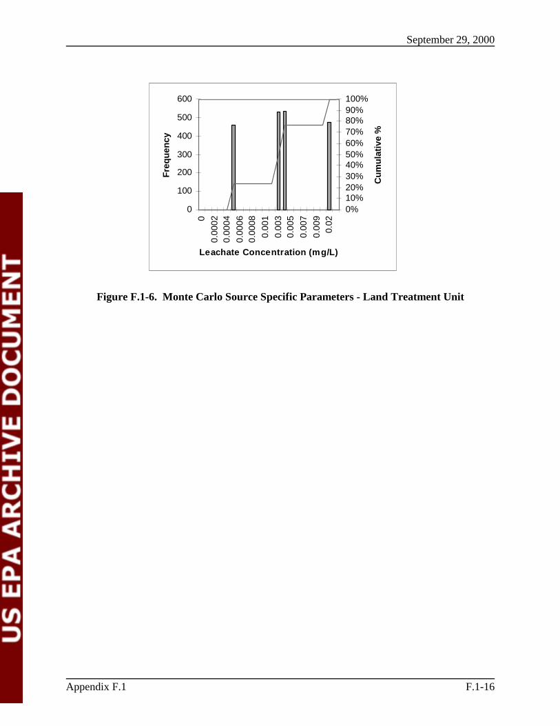
September 29, 2000

Appendix F.1 F.1-16

0

100

200

300

400

500

600

0

0.00

020.

0004

0.00

060.

0008

0.00

1

0.00

30.

005

0.00

7

0.00

90.

02

Leachate Concentration (mg/L)

Fre

quen

cy

0%10%20%30%40%50%60%70%80%90%100%

Cum

ulat

ive

%

Figure F.1-6. Monte Carlo Source Specific Parameters - Land Treatment Unit

September 29, 2000

Appendix F.1 F.1-17

0

50

100

150

200

250

300

350

400

0.E

+00

5.E

-12

5.E

-11

5.E

-10

5.E

-09

5.E

-08

5.E

-07

5.E

-06

5.E

-05

2.E

-04

4.E

-04

6.E

-04

8.E

-04

1.E

-03

3.E

-03

Average Receptor Well Concentration (mg/L)

Fre

quen

cy

0%

10%

20%

30%

40%

50%

60%

70%

80%

90%

100%

Cum

ulat

ive%

0

100

200

300

400

500

600

0.E

+00

5.E

-10

5.E

-09

5.E

-08

5.E

-07

5.E

-06

5.E

-05

2.E

-04

4.E

-04

6.E

-04

8.E

-04

1.E

-03

3.E

-03

Average Receptor Well Concentration(mg/L)

Fre

quen

cy

0%

10%

20%

30%

40%

50%

60%

70%

80%

90%

100%

Cum

ulat

ive

%

Figure F.1-7a. Chlorinated Aliphatics, Landfill Scenario , Monte Carlo OutputDistribution for Average Receptor Well Concentrations for Arsenic

Figure F.1-7b. Chlorinated Aliphatics, Land Treatment Unit , Monte Carlo OutputDistribution for Average Receptor Well Concentrations for Arsenic

September 29, 2000

Appendix F.1 F.1-18

References

API (American Petroleum Institute), 1989.Hydrogeologic Database for GroundwaterModeling. API Publication No. 4476, American Petroleum Institute.

Heath, R.C. 1984.State Summaries of Groundwater Resources. United States GeologicalSurvey Water-Supply Paper 2275.

U.S. EPA (Environmental Protection Agency). 1997a.EPA's Composite Model for LeachateMigration with Transformation Products (EPACMTP) User's Guide. Office of SolidWaste, Washington, DC.

U.S. EPA (Environmental Protection Agency). 1997b.Analysis of Subtitle D WasteManagement Units Databases Used in the Groundwater Pathway Analysis for HWIR.Office of Solid Waste, Washington, DC.

September 29, 2000

8-1

8. ERRATA

The following sections present errors that we noted in the 1999 Risk Assessment

Technical Background Document. None of these errors changes the outcome of the analysis,

but the corrections are presented here for the sake of completeness. In cases where errors

were noted in tables, we provide revised tables, and indicate the modified information by

double-underline or by a double-lined cell border.

Section 2

1. p. 2-10. Table 2-2. The analytical result shown for the TCLP arsenic concentration for

sample OC-02 is incorrect. The value should be shown as <0.0025, half of the detection limit

(0.005), rather than as <0.005. The central tendency arsenic TCLP concentration should be

calculated as 0.0186 mg/L, rather than 0.0193 mg/L. The correct concentrations were used in

EPA’s risk analyses, the values were only reported incorrectly on the table.

2. p. 2-11. Table 2-2. Our analyses always consider the concentrations of each of the specific

congeners since the congeners have different fate and transport properties. Consequently, the

results for “Total TCDF,” “Total HxCDF,” and “Total HpCDF” reported by the laboratory are

superfluous and should be disregarded.

3. p. 2-26, 3rd paragraph. Although the specific infiltration rates that we used in our

groundwater analyses are presented in Appendix K, this paragraph should clarify that in

conducting the groundwater fate and transport modeling for the deterministic EDC/VCM landfill

analysis, we used infiltration rate data from the Brownsville meteorological station to represent

our central tendency site location, Houston. Brownsville was the meteorological station closest

to Houston for which we had data. We also used the Brownsville infiltration rate data in lieu of

the Houston meteorological station in our probabilistic groundwater pathway risk analyses. The

Houston meteorological station was used as the central tendency location for all of our non-

groundwater modeling. Houston subsurface parameters were used as central tendency in the

groundwater modeling.

September 29, 2000

8-2

4. p. 2-32. Fisher Scenario. This section says that the distance to the stream was fixed at

102m from the source. However, stream distance actually was varied in the deterministic

analyses (that is, stream distance was included as a sensitive parameter in the sensitivity

analyses). The stream distances evaluated were 102m and 300m for the chlorinated aliphatics

wastewater tank, EDC/VCM landfill, and methyl chloride landfill scenarios, and 102m and 403m

for the EDC/VCM land treatment unit scenario. The impact of the difference in the analysis as

described and as implemented is provided in more detail in the discussion of Appendix D.5,

below.

5. p. 2-36. Figure 2-5. Some information was left off of the figure as it appeared in the 1999

document. The revised figure is presented on the following pages.

6. p. 2-39, 3rd bullet. Manganese should be deleted from the list of constituents we did not

evaluate because they are essential nutrients. Manganese was included in our analyses.

7. pp. 2-40 through 2-43. Table 2-8. Several errors were noted in Table 2-8. A revised

version of Table 2-8 is provided on the following pages.

8-3

Resident (adult & child)Home gardenerFarmer (adult & child)Recreational fisher

Resident (adult & child)Home gardenerChild of farmerRecreational fisher

Resident (adult & child)Home gardenerFarmer (adult & child)Recreational fisher

Land TreatmentUnit

Runoff/Erosion

Infiltration

Watershed

Groundwater

Runoff/Erosion

Groundwater

AgriculturalField

HomeGarden

SurfaceWater

Airborne Vapors/Particulates

Surface Soil(Backyard)

Deposition/Diffusion

Dispersion

SurfaceWater

AirborneParticulates

AirborneVapors

Resuspension

Volatilization

Ingestion of drinking waterInhalation from householdwaster useDermal contact while showering

Ingestion of fruits & vegetablesIngestion of beefIngestion of dairyIngestion of soil a

Ingestion of fruits & vegetables

Ingestion of fish

Inhalation of vaporsInhalation of particulates

Ingestion of soil

PrimaryRelease

Mechanism(s)

SecondarySource(s)

SecondaryRelease

Mechanism(s)

MigrationPathway(s)

ExposureRoute(s)

Notes: Complete pathway evaluateda Adult farmer only

Farmer (adult & child)

Home gardener

Recreational fisher

PotentialReceptor(s)

Figure 2-5 (Revised). Exposure Pathways - Wastewater Treatment SludgeManaged in an On-Site Land Treatment Unit

8-4

Table 2-8 (REVISED). COPCs for Chlorinated Aliphatics Wastewaters, EDC/VCM Sludges, and Methyl Chloride Sludges

Constituent CAS No.

ChlorinatedAliphatics

Wastewaters EDC/VCM Sludges Methyl Chloride Sludges

Non-Groundwater

Pathways

GroundwaterPathways

NongroundwaterPathways

GroundwaterPathways

Non-Groundwater

PathwaysLTU Landfill LTU LandfillVolatile Organics1,2-Dichloroethane 107062 X g X X X2-Chloro-1,3-butadiene 126998 XAcetone 67641 X g g X X g XAllyl chloride 107051 X g X XBromoform 75252 j* gCarbon disulfide 75150 X g g X X gChlorobenzene 108907 XChloroethane 75003 XChloroform 67663 X g X X Xcis-1,2-Dichloroethylene 156592 Xcis-1,3-Dichloropropene 10061015 XChlorodibromomethane 124481 j*Ethylbenzene 100414 X2-Hexanone 591786 j j jMethyl ethyl ketone 78933 X g g X XMethylene chloride 75092 j* g X X X g XStyrene 100425 XTetrachloroethylene 127184 X g,j j* j*trans-1,2-Dichloroethylene 156605 j*Trichloroethylene 79016 X g,j j* j*Vinyl Chloride 75014 g,j j* j*Vinyl Acetate 108054 g X X

(continued)X = Constituent of Potential Concern.g = Constituent screened out of the groundwater pathway analysis.v = Constituent screened out of the nongroundwater pathway analysis (only the vapor air pathway was evaluated).e = Essential nutrient.j = All values were non-detect, with the exception of one “J”-qualified (estimated) value; “*” indicates that although screened out, the constituent wasretained in the analysis inadvertently.

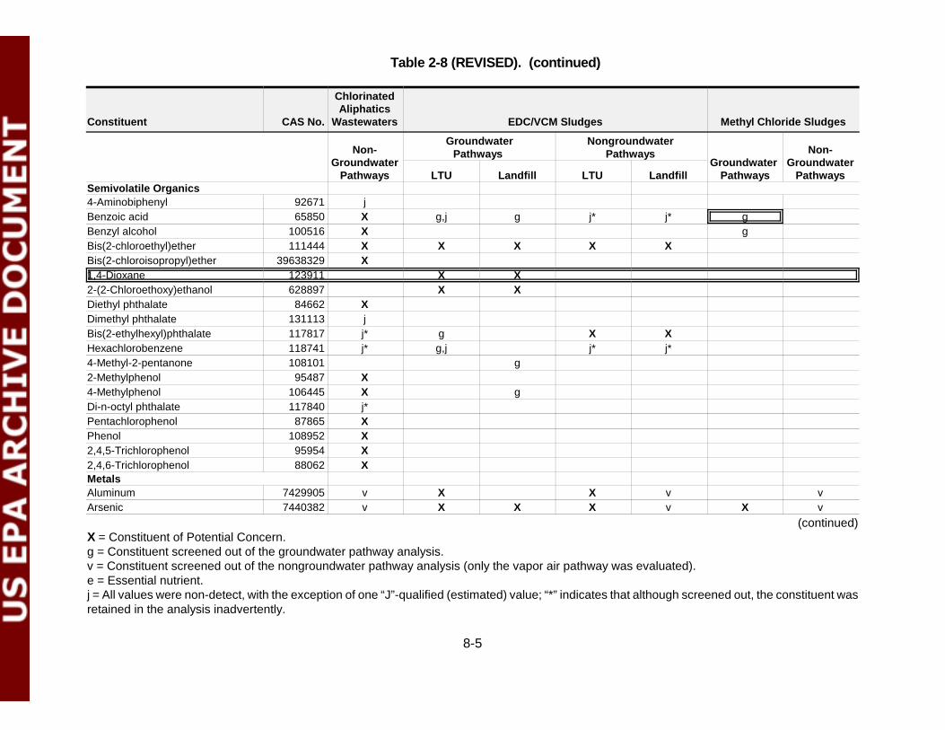
Constituent CAS No.



Non-Groundwater

Pathways

GroundwaterPathways


GroundwaterPathways

Non-Groundwater

PathwaysLTU Landfill LTU Landfill

8-5

Table 2-8 (REVISED). (continued)

Semivolatile Organics4-Aminobiphenyl 92671 jBenzoic acid 65850 X g,j g j* j* gBenzyl alcohol 100516 X gBis(2-chloroethyl)ether 111444 X X X X XBis(2-chloroisopropyl)ether 39638329 X1,4-Dioxane 123911 X X2-(2-Chloroethoxy)ethanol 628897 X XDiethyl phthalate 84662 XDimethyl phthalate 131113 jBis(2-ethylhexyl)phthalate 117817 j* g X XHexachlorobenzene 118741 j* g,j j* j*4-Methyl-2-pentanone 108101 g2-Methylphenol 95487 X4-Methylphenol 106445 X gDi-n-octyl phthalate 117840 j*Pentachlorophenol 87865 XPhenol 108952 X2,4,5-Trichlorophenol 95954 X2,4,6-Trichlorophenol 88062 XMetalsAluminum 7429905 v X X v vArsenic 7440382 v X X X v X v


Constituent CAS No.



Non-Groundwater

Pathways

GroundwaterPathways


GroundwaterPathways

Non-Groundwater


8-6


Barium 7440393 v g X vBeryllium 7440417 vCadmium 7440439 v g X vCalcium 7440702 v e e e v e vChromium 7440473 v g X v vCobalt 7440484 v g g X vCopper 7440508 v X X X v X vIron 7439896 v e e v vLead 7439921 v X X v vMagnesium 7439954 v e e e v e vManganese 7439965 v g X X v g vMercury 7439976 XMolybdenum 7439987 v g X X vNickel 7440020 v g X X v vPotassium 7440097 v e e e vSodium 7440235 v e e vVanadium 7440622 v g X vZinc 7440666 v g g X v g vDioxins/Furans1,2,3,4,6,7,8-HpCDD 35822469 X g X X X1,2,3,4,6,7,8-HpCDF 67562394 X g X X X X1,2,3,4,7,8,9-HpCDF 55673897 X g X X X1,2,3,4,7,8-HxCDD 39227286 X g X X


Constituent CAS No.



Non-Groundwater

Pathways

GroundwaterPathways


GroundwaterPathways

Non-Groundwater


8-7


1,2,3,6,7,8-HxCDD 57653857 X g X X1,2,3,7,8,9-HxCDD 19408743 X g X X1,2,3,4,7,8-HxCDF 70648269 X g X X1,2,3,6,7,8-HxCDF 57117449 X g X X1,2,3,7,8,9-HxCDF 72918219 X g X X2,3,4,6,7,8-HxCDF 60851345 X g X X2,3,4,7,8-PeCDF 57117314 X g X X1,2,3,7,8-PeCDF 57117416 g X X2,3,7,8-TCDD 41903575 X g X X2,3,7,8-TCDF 51207319 X g X XOCDD 3268879 X g X X X XOCDF 39001020 X g X X X XX = Constituent of Potential Concern.g = Constituent screened out of the groundwater pathway analysis.v = Constituent screened out of the nongroundwater pathway analysis (only the vapor air pathway was evaluated).e = Essential nutrient.j = All values were non-detect, with the exception of one “J”-qualified (estimated) value; “*” indicates that although screened out, the constituentwas retained in the analysis inadvertently.

Notes:1 OCDD was screened out of the groundwater pathway analysis for the landfill, but was retained in the analysis inadvertently.

September 29, 2000

8-8

Section 3

1. p. 3-1, 2nd paragraph. The last sentence should be changed to "The partitioning equations

used to estimate volatilization from the source are based on equations presented in a series of

articles by Jury et al. (Jury et al., 1983, 1984, and 1990)."

2. p. 3-1, 3rd paragraph, 1st sentence. “erosion and” should be deleted from the sentence

because the source partition model does not predict mass losses from erosion.

3. p. 3-2, 3rd paragraph. The third sentence of the paragraph was truncated and only

referenced three congeners for which we capped concentrations a their solubility

concentrations, not four. Further, the sentence can be re-written for additional clarity, as

follows: “Consequently, for both the deterministic and probabilistic analyses, we constrained the

overall influent contaminant load to the wastewater treatment system based on the aqueous

solubility of the four congeners with sample concentrations that exceeded their respective

solubility limits: 1,2,3,4,6,7,8-HpCDF, OCDD, OCDF, and 1,2,3,4,7,8,9-HpCDF.

4. p. 3-6, Table 3-1b. 1) The heading for the third column should read “GL-02" where it reads

“G(ng/L)”. 2) Some values in four of the table rows were incorrect; however, the values actually

used in the analysis were correct, and the error does not have any actual impact on the

computed results. 3) The “Note” at the bottom of the table should include 1,2,3,4,6,7,8-HpCDF

in the list of the congeners that were capped at their solubility limits. A revised version of Table

3-1b is included on the following page.

5. p. 3-11, Table 3-2. “LF Area” refers to the “landfill area” being the high-end parameter of

concern. X-well refers to the longitudinal distance to the well and Y-well refers to the lateral

distance to the well from the plume center line. The column entitled “Waste Volume” indicates

the waste volume in the landfill that was used in the fate and transport modeling for the

particular model run that is defined by that row in the table. As indicated in the waste volume

column, the central tendency waste volume is 15,202 m3, and the high end value is 50,579 m3.

6. p. 3-16, 3rd paragraph, 5th sentence. The MCL for mercury is 0.002 mg/L, not 0.005 mg/L.

8-9

Table 3-1b (Revised). Estimated High End Dioxin Congener Emissions from Wastewater Tanks

Congener

TEF

GL-02

Concentration

(ng/L)

Annual

Quantity

(g/yr) a

Annual TEQ

Quantity

(g/yr) a

Annual

Emissions

(Mg/yr)

Annual

Emissions

(g/yr)

Annual TEQ

Emissions

(g/yr)

1,2,3,4,6,7,8-HpCDD 0.01 0.880 0.283 0.0028 4.03e-10 4.03e-04 4.03e-06

1,2,3,4,6,7,8-HpCDF 0.01 43.0 13.844 0.1384 6.92e-09 6.92e-03 6.92e-05

1,2,3,4,7,8,9-HpCDF 0.01 12.0 3.863 0.0386 6.92e-09 6.92e-03 6.92e-05

1,2,3,4,7,8-HxCDD 0.1 0.052 0.017 0.0017 7.25e-11 7.25e-05 7.25e-06

1,2,3,6,7,8-HxCDD 0.1 0.091 0.029 0.0029 2.65e-10 2.65e-04 2.65e-05

1,2,3,7,8,9-HxCDD 0.1 0.110 0.035 0.0035 3.20e-10 3.20e-04 3.20e-05

1,2,3,4,7,8-HxCDF 0.1 5.30 1.706 0.1706 1.80e-08 1.80e-02 1.80e-03

1,2,3,6,7,8-HxCDF 0.1 1.20 0.386 0.0386 1.80e-09 1.80e-03 1.80e-04

1,2,3,7,8,9-HxCDF 0.1 0 0 0 0 0 0

2,3,4,6,7,8-HxCDF 0.1 0.430 0.138 0.0138 1.05e-09 1.05e-03 1.05e-04

2,3,4,7,8-PeCDF 0.5 0.210 0.068 0.0338 5.96e-10 5.96e-04 2.98e-04

2,3,7,8-TCDD 1 0.017 0.005 0.0055 6.30e-11 6.30e-05 6.30e-05

2,3,7,8-TCDF 0.1 0.082 0.026 0.0026 5.77e-10 5.77e-04 5.77e-05

OCDD 0.001 6.90 2.221 0.0022 7.79e-14 7.79e-08 7.79e-11

OCDF 0.001 6,000 1931.676 1.9317 5.52e-11 5.52e-05 5.52e-08

Total 1954.300 2.387 0.037 0.003

% Total 0.002% 0.11%

a Based on central tendency annual waste quantity of 321,946 m3 or metric tons.

Note: The TEQ emissions estimates presented in this table are based on the solubility limits for 1,2,3,4,6,7,8-HpCDF,

1,2,3,4,7,8,9-HpCDF, OCDD, and OCDF (see Appendix C), and the sample concentrations in the PL-01 and GL-02 samples for the other

congeners.

September 29, 2000

8-10

Section 4

1. pp. 4-5 and 4-5, Tables 4-1 and 4-2. Some of the entries in the table were incorrect (rows of

the table were shifted in the version of the table presented in the 1999 Risk Assessment TBD).

Revised tables are provided on the following pages. The child exposure factors are correct as

presented in Appendix K.

2. p. 4-10, 1st paragraph. The last two sentences of this paragraph are incorrect and should be

deleted.

3. p. 4-13, Table 4-4. The high end concentrations for chlorinated aliphatics wastewaters were

incorrect as presented in the 1999 Risk Assessment TBD (the concentrations presented

correspond to a distance to receptor of 75m). The correct concentrations were presented in

Table H.1-1a of Appendix H.1 in the 1999 document. In addition, two values were updated to

be consistent with a revised version of the source document.

4. p. 4-17. Section 4.2.4. 2-(2-chloroethoxy)ethanol should have been included in the list of

constituents for which no toxicity values are available.

5. p. 4-19, 2nd bullet. The word “and” after “sludge” should be deleted.

6. p. 4-19, 1st paragraph. The sentence: “The concentration of lead in chlorinated aliphatics

wastewater exceeds this concentration, as well as the background concentrations reported by

Hunter (1998)” should be deleted. In our analysis of wastewaters we were only concerned with

vapor emissions. The evaluation of lead is not relevant to the analysis. The text should note,

however, that the leachate concentration predicted for the land treatment unit based on sludge

dry weight concentrations, 0.005 mg/L (USEPA, 1999, Appendix B, Table B-1), is well below the

action level for lead in drinking water (0.015 mg/L).

8-11

Table 4-1 (Revised). Time-weighted Average (TWA) Intake Rates for Central Tendency Child Receptor

Parameter Units Data source aAge

Group1-2

AgeGroup

3-5

AgeGroup6-11

AgeGroup12-19

CalculatedTWA

TWA Units Comments

Soil ingestion rate kg/d Table 4-23 0.0001 0.0001 0.00005 0.00005 2.70E-06 kg/kg/d

Drinking wateringestion rate

L/kg/d Tables 3-7 &3-30

0.0305 0.0163 2.38E-02 L/kg/d ages 1 - 10 and 11 - 19

Fruit ingestion rate g DW/kg/d Table 9-7 &13-61

0.432 0.271 0.165 0.0907 1.79E-04 kg DW/kg/d WW concentrations inEFH converted to DW

Vegetable ingestionrate

g DW/kg/d Table 13-63 0.166 0.102 0.0566 0.0577 7.58E-05 kg DW/kg/d WW concentrations inEFH converted to DW

Root ingestion rate g DW/kg/d Table 13-65 0.92 0.462 0.523 0.565 5.73E-04 kg DW/kg/d WW concentrations inEFH converted to DW

Root ingestion rate g WW/kg/d calculated 0.131 0.066 0.074 0.080 8.16E-05 kg WW/kg/d

Dairy ingestion rate g DW/kg/d Table 11-2 23.48 19.52 11.88 5.29 1.15E-02 kg DW/kg/d WW concentrations inEFH converted to DW

Dairy ingestion rate g WW/kg/d calculated 5.635 4.685 2.851 1.270 2.77E-03 kg WW/kg/d

Beef ingestion rate g DW/kg/d Tables 11-3 &13-36

1.339 1.162 2.11 1.51 1.63E-03 kg WW/kg/d WW concentrations inEFH converted to DW

Beef ingestion rate g WW/kg/d calculated 0.380 0.330 0.599 0.429 4.62E-04 kg WW/kg/d

Inhalation rate m3/d Myers et al. 1998,Table 5-2

5.4 8.6 12 3.15E-01 m3/kg/d ages 0 - 3, 4 - 10, 11 - 18

Average body weightfor soil ingestion

kg Tables 7-6 & 7-7 12.15 17.13 29.48 56.61 kg used to calculate TWA forsoil ingestion

Average body weightfor inhalation

kg Tables 7-6 & 7-7 12.13 24.91 53.55 kg used to calculate TWA forinhalation

DW = dry weightWW = wet weighta Tables are found in the Exposure Factors Handbook (EFH)

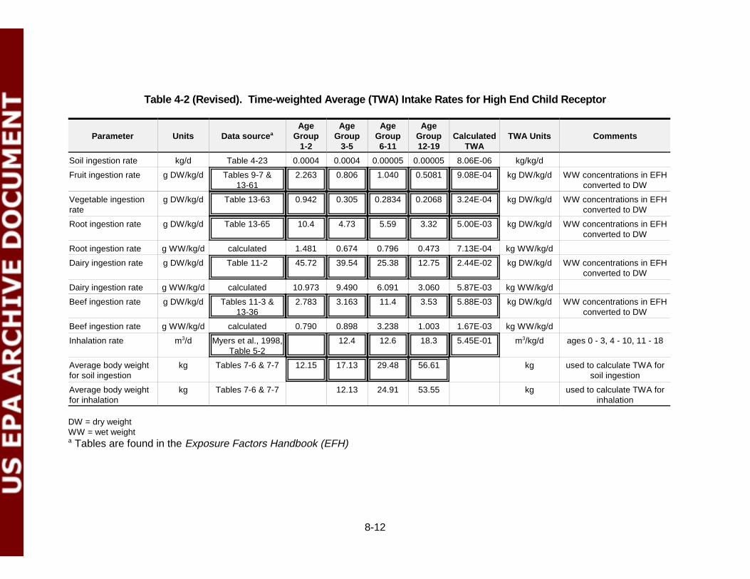
8-12

Table 4-2 (Revised). Time-weighted Average (TWA) Intake Rates for High End Child Receptor

Parameter Units Data source aAge

Group1-2

AgeGroup

3-5

AgeGroup6-11

AgeGroup12-19

CalculatedTWA

TWA Units Comments

Soil ingestion rate kg/d Table 4-23 0.0004 0.0004 0.00005 0.00005 8.06E-06 kg/kg/d

Fruit ingestion rate g DW/kg/d Tables 9-7 &13-61

2.263 0.806 1.040 0.5081 9.08E-04 kg DW/kg/d WW concentrations in EFHconverted to DW

Vegetable ingestionrate

g DW/kg/d Table 13-63 0.942 0.305 0.2834 0.2068 3.24E-04 kg DW/kg/d WW concentrations in EFHconverted to DW

Root ingestion rate g DW/kg/d Table 13-65 10.4 4.73 5.59 3.32 5.00E-03 kg DW/kg/d WW concentrations in EFHconverted to DW

Root ingestion rate g WW/kg/d calculated 1.481 0.674 0.796 0.473 7.13E-04 kg WW/kg/d

Dairy ingestion rate g DW/kg/d Table 11-2 45.72 39.54 25.38 12.75 2.44E-02 kg DW/kg/d WW concentrations in EFHconverted to DW

Dairy ingestion rate g WW/kg/d calculated 10.973 9.490 6.091 3.060 5.87E-03 kg WW/kg/d

Beef ingestion rate g DW/kg/d Tables 11-3 &13-36

2.783 3.163 11.4 3.53 5.88E-03 kg DW/kg/d WW concentrations in EFHconverted to DW

Beef ingestion rate g WW/kg/d calculated 0.790 0.898 3.238 1.003 1.67E-03 kg WW/kg/d

Inhalation rate m3/d Myers et al., 1998,Table 5-2

12.4 12.6 18.3 5.45E-01 m3/kg/d ages 0 - 3, 4 - 10, 11 - 18

Average body weightfor soil ingestion

kg Tables 7-6 & 7-7 12.15 17.13 29.48 56.61 kg used to calculate TWA forsoil ingestion

Average body weightfor inhalation

kg Tables 7-6 & 7-7 12.13 24.91 53.55 kg used to calculate TWA forinhalation

DW = dry weightWW = wet weighta Tables are found in the Exposure Factors Handbook (EFH)

8-13

Table 4-4 (Revised). Comparison of Background Concentrations and Intake Rates of Dioxin to Concentrations andIntake Rates Associated with Chlorinated Aliphatics Wastes

Comparison of Dioxin Concentrations and Dioxin Daily Intakes: Background vs. Chlorinated Aliphatics Wastes

Dioxin Source

Average BackgroundChlorinated Aliphatics Wastes

( Adult Farmer Scenario)

Source: “EstimatingExposure to Dioxin-Like

Compounds”(U.S. EPA 1994)

Source: “DioxinFactsheet: BackgroundEnvironmental Levels

and Exposure”(U.S. EPA 1999, updated)

Chlorinated AliphaticsWastewater

(Incremental Risk)EDC/VCM

Land Treatment Unit

CentralTendency

HighEnd

CentralTendency

HighEnd

TEQ in waste 0.313 ng/L 7.414 ng/L 78.9 ng/kg 907 ng/kg

TEQ in soil 8 ng/kg(n=95)

Rural: 1 to 6 ng/kgUrban: 7 to 20 ng/kg

0.0011 ng/kg 0.007 ng/kg 5.4 ng/kg 61 ng/kg

TEQ in beef 0.29 ng/kg[0.48 ng/kg]*

(n=14)

0.17 ng/kg 0.011 ng/kg 0.12 ng/kg 0.13 ng/kg 1.4 ng/kg

TEQ in dairy Milk 0 ng/kg[0.07 ng/kg](n=2)

Other Dairy 0.35 ng/kg[0.36 ng/kg](n=5)

Egg 0.0004 ng/kg[0.13 ng/kg](n=8)

Milk 0.03 ng/kg

Other Dairy 0.1 ng/kg

Egg 0.03 ng/kg

0.0032 ng/kg 0.03 ng/kg 0.030 ng/kg 0.32 ng/kg

TEQ in air 0.0949 pg/m3

(n=84)Rural: 0.002 to 0.02 pg/m3

Urban: 0.02 to 0.2 pg/m30.00032 pg/m3 0.002 pg/m3 NA NA

TEQ DioxinIntake

mean: 0.062 ng/d[0.119 ng/d]

0.070 ng/d WHO TEQdue to dioxins,furans,PCBs

0.0012 ng/d* 0.012 ng/d* 0.012 ng/d* 0.13 ng/d*

* Based on central tendency intake rates (and assumptions regarding the fraction of a farmer’s food that is home-grown).n = number of samplesNA = not calculated[ ] = For 1994 data, values in [brackets] based on ND = 0.5DL

September 29, 2000

8-14

Section 5

1. p. 5-12, Table 5-1b. “Age 12-18" should read “Age 12-19.”





6. p. 5-29, Item 4, 2nd sentence. “average” should read “median.”

Appendix C

1. Appendix C, Table C-31, Tetrachloroethylene and Table C-32, Trichloroethylene. For these

two contaminants we incorrectly used cancer slope factors and unit risk factors that did not

meet our selection criteria (benchmarks provided by IRIS, HEAST, NCEA, or CalEPA). These

values should be deleted. There are no cancer slope factors or unit risk factors for these that

meet our criteria for selecting benchmarks.

2. Appendix C, Table C-37, 2,3,7,8-TCDD. We incorrectly cited HEAST as the source of the

slope factor for 2,3,7,8-TCDD. The source of this slope factor actually is:

“USEPA, 1985. Health Assessment Document for Polychlorinated Dibenzo-p-Dioxins. Office of

Health and Environmental Assessment. EPA/600/8-84/014F. September.”

A risk estimate calculated using the slope factor presented in HEAST would be only a factor of

0.96 (150,000/156,000) times a risk estimate calculated based on the slope factor presented in

the 1985 document. This difference would have no discernable impact on our risk estimates.

September 29, 2000

8-15

Appendix D.5

1. Section 2 of the 1999 Risk Assessment TBD said that the distance to the stream was

fixed at 102 m from the source. However, stream distance actually was varied in the

deterministic analyses (included as a sensitive parameter in the sensitivity analyses). The

stream distances evaluated were 102 m and 300 m for the chlorinated aliphatics wastewater

tank and EDC/VCM and methyl chloride landfill scenarios, and 102 m and 403 m for the

EDC/VCM land treatment unit scenario. In addition, the discussion of the surface water model

in Appendix D.5 of the 1999 Risk Assessment TBD suggested that we evaluated two stream

orders, a high end stream of reach order 3 and a central tendency stream of reach order 5, in

the sensitivity analyses for the fisher scenario. In reality, we only evaluated a stream order 3 in

our fisher analysis. The rationale for selecting an order 3 stream as the fishable waterbody was

based primarily on the desire to create an exposure scenario that was protective of different

types of fishable waterbodies and, at the same time, representative of streams on a national

basis (that is, streams of order 3 are much more prevalent on a national basis than streams of

orders 4 and above).

After identifying these errors in the text, we investigated the impact of allowing the

stream distance to vary and of evaluating only an order 3 stream in the deterministic analyses.

Our evaluation of the risk estimates found that modifying the analysis consistent with the

manner in which it is described in the 1999 Risk Assessment TBD would not result in any

meaningful difference in the risk or hazard estimates. Specifically, high risk and hazard

quotient estimates due to fish ingestion would be modified as follows:

• For the EDC/VCM LTU, the sum of the COPC high end risk estimates due to fishingestion are 2E-05 and 9E-12 due to nongroundwater and groundwater pathways,respectively. The nongroundwater pathway risks are due to dioxins. The sum of theCOPC high end hazard quotients due to nongroundwater pathways is 0.003 (there areno groundwater COPCs for which HQs are calculated). Modifying the analysis toevaluate a reach order 5 stream rather than a reach order 3 stream decreases the fishingestion risk estimates by a maximum factor of 30. Evaluating a distance of 403minstead of 102m increases the fish ingestion risk estimates by a maximum factor of 1.25.This phenomenon is a function of the model construct used to simulate overlandtransport of contaminant through runoff and erosion of contaminant sorbed to soilparticles. For constituents that sorb strongly to soil particles, decreasing the distance toreceptor effectively decreases the area of the drainage subbasin, resulting in a slightdecrease of the overall load due to soil erosion to the stream (see Appendix D.2 for

September 29, 2000

8-16

additional details on the overland transport model). In some instances, the risk resultsincreased with decreasing distance to stream and, in other cases, (e.g., for dioxincongeners) the risk results decreased slightly with decreasing distance to the stream.

• For the EDC/VCM landfill, the sum of the COPC high end risk estimates due to fishingestion are 7E-15 and 1E-10, due to nongroundwater and groundwater pathways,respectively. The sum of the COPC high end hazard quotients due to fish ingestion are<0.0001 and 0.0000002, due to nongroundwater and groundwater pathways,respectively. For the nongroundwater pathways, modifying the analysis to evaluate areach order 5 stream rather than a reach order 3 stream increases the fish ingestion riskestimates and hazard quotients by a maximum factor of 1.25. Evaluating a distance of300m instead of 102m increases the fish ingestion risk estimates and hazard quotientsby a maximum factor of 1.1. For the groundwater pathways, modifying the analysis toevaluate a reach order 5 stream rather than a reach order 3 stream decreases the fishingestion risk estimates and hazard quotients by a maximum factor of 30. Evaluating adistance of 102m instead of 430m increases the fish ingestion risk estimates and hazardquotients by a maximum of 3 orders of magnitude.

For the nongroundwater pathway, the increase in risk estimates/hazard quotients with alarger stream is counterintuitive because one would expect there to be greater dilution ofcontaminants in a larger stream. However, because we did not average the depositionrate over the entire area of the stream (a single point estimate of deposition was usedfor the entire surface area of the stream) we created an artificially high load ofcontaminant deposition to the reach order 5 stream. That is, the maximum depositionrate would have been set for the entire surface water area which, for reach order 5streams, is over one million meters squared. Given this situation, the volumetric dilutionof the contaminant would be offset by an artificially high average deposition rate suchthat the risk estimates for an order 5 reach could actually increase. This is particularlytrue for highly hydrophobic constituents because the dry vapor phase constituentdiffusion load to the waterbody (LDif in equation E-4.12) is, in part, driven by the Henry’sLaw constant. As shown in that equation, the diffusion load tends to be higher forconstituents with low values of Henry’s Law constant (as with dioxins and otherhydrophobic constituents). For a reach order 3 stream, the use of a single pointprovides a reasonable approximation of the deposition onto the stream.

• For the chlorinated aliphatic wastewater tank, the sum of the COPC high end riskestimates due to fish ingestion is 1E-10. The sum of the COPC high end hazardquotients due to fish ingestion is 0.01. Modifying the analysis to consider a reach order5 stream rather than a reach order 3 stream increases the fish ingestion risk estimatesand hazard quotients by a maximum factor of 1.5. Evaluating a distance of 300minstead of 102m increases the fish ingestion risk estimates and hazard quotients by amaximum factor of 1.2.

• For the methyl chloride landfill, the sum of the COPC high end risk and hazard quotientestimates due to fish ingestion are 4E-16 and <0.0001, respectively. These estimateswould have to be modified many orders of magnitude to be of concern. Consequently,the difference in our analysis as presented in the 1999 Risk Assessment TBD and asconducted has no impact on the methyl chloride landfill fisher results.

September 29, 2000

8-17

These analyses demonstrate that modifying our evaluation of fisher receptor in a

manner consistent with the methodology described in the 1999 Risk Assessment TBD would

not result in any meaningful change in the risk estimates or hazard quotients calculated for the

fisher.

Appendix F

1. p. F.2-7. The fish ingestion rate listed as corresponding to "all ages" should be changed to

“adult.”

Appendix H

1. pp. H.3-34 and H.3-35, Tables H.3-6a and H.3-6b. The titles of these tables should indicate

that they present probabilistic risk results for arsenic.

Appendix K

1. In Table K-3, in the column labeled Source for Minimum and Maximum Values (If different

from the Data Source) all references to EPACMTP should be removed. All but two of these

should be left blank because the source for the minimum and maximum are in fact the same as

the data source. The exceptions are:

(1) under Saturated zone parameters, for Seepage Velocity (pore

porosity), the source for minimum and maximum values should

read Minimum and maximum values based on survey data

reported by Newell et al., 1990 (Groundwater 28(5), p. 703-714),

and

(2) under Unsaturated zone parameters, for Saturated

conductivity of the soil, the source for minimum and maximum

values should read Minimum value set to 1.5E-04 to avoid

infeasible zero value.

September 29, 2000

8-18

2. In Table K-3, the Bulk density and Porosity parameters for the EDC/VCM landfill and the

EDC/VCM LTU should be changed to read yes rather than no under the column Monte Carlo

Variable. They currently read no because the values are not randomly generated from a

distribution but rather are derived from data that are randomly generated. We believe that yes

more accurately describes the modeling performed.

3. In Table K-4, the reference for Beef intake under both the Child of Farmer (1-5 years) and

Child of Farmer (6-11 years) should be changed from . . . EFH Table 13-61 . . . to . . . EFH

Table 13-36 . . .

4. In Table K-1, under Tank Parameters, the units for Impeller diameter should be changed

from unitless to cm.

5. In table K-1, for the EDC/VCM Wastewater Treatment Sludge Managed in an Off-site

Landfill, under Surface and Subsurface Soil Parameters (Unsaturated Zone) a footnote should

be added to the central tendency value for Unsaturated zone thickness (depth to water table)

which should read Unsaturated zone thickness is a location-specific parameter. The

unsaturated zone thickness values presented correspond to the central tendency and high-end

locations and are varied with location, not independently.

6. In Table K-1, for the Methyl Chloride Wastewater Treatment Sludge Managed in an On-site

Landfill, because groundwater modeling was not performed, all checkmarks under the

EPACMTP column should be removed. It follows that the entire row for Average soil pH and

Residual water content should be deleted as the only checkmarks that were included for these

parameters were for EPACMTP.


Landfill under Landfill Parameters the central tendency for Type of daily cover should be

changed from Soil to NA because no daily cover is assumed.

September 29, 2000

8-19


Landfill under Meteorological Parameters, for the Mean annual wind speed, the checkmark

under EPACMTP should be removed and a checkmark should be added under ISC.

9. In Table K-1, for EDC/VCM Waste Managed in a Land Treatment Unit, under Surface and

Subsurface Soil Parameters (Unsaturated Zone) a checkmark should be added in the

Partitioning column for the Soil bulk density parameter.

10. In Table K-1, under “Wasterwaters” Managed in Aerated Tanks, “Wasterwaters” should be

changed to “Wastewaters”. All checkmarks under Partitioning should be removed and a

checkmark should be placed under the CHEMDAT8 column for the Waste concentration

parameter. The units for Waste concentration should be changed to mg/L.

11. In Table K-1, under Constants used in Fate and Transport Modeling, under Surface Water /

Fish Parameters, the parameters Width of waterbody, Length of waterbody, and Total

waterbody depth should all have checkmarks in the Indirect Exp. column.

12. For Table K-3, all of the variables are Monte Carlo Variables, consequently the column

Monte Carlo Variable should be deleted. Because there are no constants under the Minimum,

Maximum, or Constant columns, the cell that contains -or- Constant should be removed.

13. For Table K-3, for EDC/VCM Wastewater Treatment Sludge Managed in an Off-site

Landfill, under Waste Parameters the checkmark under EPACMTP should be removed for the

Contaminant concentration parameter. Also, the checkmark under Indirect Exp. for the Fraction

organic carbon parameter should be removed.

14. For Table K-3, for EDC/VCM Wastewater Treatment Sludge Managed in an Off-site

Landfill, under Saturated Zone Parameters, the parameter Groundwater Temperature should

be removed since it is not varied.

September 29, 2000

8-20

15. For Table K-3, for Wastewaters Managed in Aerated Tanks, under Waste Parameters, the

checkmark under EPACMTP should be removed for the Contaminant concentration parameter

and the units should be changed to mg/L.

16. For Table K-3, for Wastewaters Managed in Aerated Tanks, under Tank Parameters, a

checkmark should be placed in the ISC column for the Surface area parameter.

17. For Table K-3, for Wastewaters Managed in Aerated Tanks, under Tank Parameters, Site-

specific should be entered in the Variable Type column for Soil saturated volumetric water

content, Saturated hydraulic conductivity, and Soil specific exponent representing water

retention.

Risk Assessment Technical Background Document for the ...

Documents

Transcript of Risk Assessment Technical Background Document for the ...