Risk and Uncertainty 2 - Columbia University

Risk and Uncertainty 2

Mark Dean

GR6211 - Microeconomic Analysis 1

Risk Aversion

• We motivated EU theory by appealing to risk aversion• Does EU imply risk aversion?• No!• Consider someone who has u(x) = x

• They will be risk neutral

• Consider someone who has u(x) = x2

• They will be risk loving

• So risk attitude has something to do with the shape of theutility function

Risk Aversion

• For this section we will think about lotteries with monetaryprizes

• Let δx be the lottery that gives prize x for sure and E (p) bethe expected value of a lottery p

DefinitionWe say that a decision maker is risk averse if, for every lottery p

δE (p) p

We say they are risk neutral if

δE (p) ∼ p

We say they are risk loving if

δE (p) p

Risk Aversion

• We can say the same thing a different way

DefinitionThe certainty equivalence of a lottery p is the amount c suchthat

δc ∼ pThe risk premium is

E (p)− c

Risk Aversion

LemmaFor a decision maker whose preferences are strictly monotonic inmoney

1 They are risk averse if and only if for any p the risk premiumis weakly positive

2 They are risk neurtal if and only if for any p the risk premiumis zero

3 They are risk loving if and only if for any p the risk premiumis weakly negative

Risk Aversion and Utility Curvature

• We have made the claim that there is a link between riskaversion and the curvature of the utility function

Risk Aversion and Utility Curvature

• We can make this statement tight

TheoremAn expected utility maximizer

1 Is risk averse if and only if u is concave

2 Is risk neutral if and only if u is linear

3 Is risk loving if and only if u is convex

Proof.Comes straight from Jensen’s inequality: for a random variable xand a concave function u

E (u(x)) ≤ u(E (x))

Risk Aversion and Expected Utility

• Note that our definition of risk aversion seems rather weak• Only talk about the comparison between risky lotteries andsure things

• We might want our definition to cover other situations• e.g. we might want a risk aversion decision maker to dislikemean preserving spreads

• The above result show that we get this ‘for free’if we applyour definition of risk aversion to EU maximizers

• If the DM is an EU maximizer then

Risk aversion ⇔Concave Utility ⇐⇒

p q for all q mean preserving spread of p

Measuring Risk Aversion

• We might want a way of measuring risk aversion from theutility function

• Intuitively, the more ‘curvy’the utility function, the more riskaverse

• How do we measure curvature?• The second derivative u′′(x)!• Is this a good measure?• No, because we can change the utility function in such a waythat we don’t change the underlying preferences, and changeu′′(x)

The Arrow Pratt Measure

• One way round this problem is to use the Arrow-Prattmeasure of absolute risk aversion

A(x) =−u′′(x)u′(x)

• This measure has some nice properties1 If two utility functions represent the same preferences thenthey have the same A for every x

2 It measures risk aversion in the sense that the following twostatements are equivalent

• The utility function u has a higher Arrow Pratt measure thanutility function v for every x

• Utility function u gives a higher risk premium than utilityfunction v for every p


• Why is it called a measure of absolute risk aversion?• To see this, let’s think of a function for which A(x) is constant

u(x) = 1− e−ax

• Note u′(x) = ae−ax and u′′(x) = −a2e−ax so A(x) = a• This is a constant absolute risk aversion (CARA) utilityfunction


• Claim: for CARA utility functions, adding a constant amountto each lottery doesn’t change risk attitues

• i.e if δx p then δx+z is preferred to a lottery p′ which addsan amount z to each prize in p

• To see this note that

u(x) ≥ ∑yp(y)u(y)

1− e−ax ≥ ∑yp(y)

(1− e−ay

)⇒ 1− e−ax ≥ 1−∑

yp(y)e−ay

e−az − e−axe−az ≥ e−az −∑yp(y)e−ay e−az

⇒ 1− e−a(x+z ) ≥∑yp(y)

(1− e−a(y+z )

)⇒ u(x + z) ≥∑

yp(y)u(y + z)

Relative Risk Aversion

• Is this a sensible property?• Maybe not• Means that you should have the same attitude to a gamblebetween winning $100 or losing $75 whether you are a studentearning $20,000 a year or a professor earning millions!

• Perhaps a more useful measure is relative risk aversion

R(x) = xA(x) = −xu′′(x)u′(x)


• An example of a Constant Relative Risk Aversion measure is

u(x) =x1−ρ − 11− ρ

• Note that u′(x) = x−ρ, u′′(x) = −ρx−ρ−1 and so R(x) = ρ

• CRRA utility functions have the property that proportionalchanges in prizes don’t affect risk attitudes

• i.e if δx p then δαx is preferred to a lottery p′ whichmultiplies each prize in p by α > 0


• To see this note that

u(x) ≥ ∑yp(y)u(y)

⇒ x1−ρ − 11− ρ

≥ ∑y p(y)y1−ρ − 1

1− ρ

⇒ x1−ρ ≥∑yp(y)y1−ρ

⇒ α1−ρx1−ρ ≥∑yp(y)α1−ρy1−ρ

⇒ (αx)1−ρ − 11− ρ

≥ ∑y p(y) (αy)1−ρ − 1

1− ρ

u(αx) ≥ ∑yp′(y)u(y)

Are People Expected Utility Maximizers?

• Because of the work we have done above, we know what the‘behavioral signature’is of EU

• The independence axiom

• Essentially this is picking up on the fact that EU demandspreferences to be linear in probabilities

• Does this hold in experimental data?

The Common Ratio Effect

• What would you choose?• Many people choose C1 and D2


• This is a violation of the independence axiom• Why?• Because

D1 = 0.25C1+ 0.75R

D2 = 0.25C2+ 0.75R

where R is the lottery which pays 0 for sure

• Thus independence means that

C1 C2⇒ D1 D2

The Common Consequence Effect

• What would you choose?• Many people choose A1 and B2

The Common Consequence Effect

Explanations

• What do you think is going on?• Many alternative models have been proposed in the literature

• Disappointment: Gul, Faruk, 1991. "A Theory ofDisappointment Aversion,"

• Salience: Pedro Bordalo & Nicola Gennaioli & Andrei Shleifer,2012. "Salience Theory of Choice Under Risk,"

• One of the most widespread and straightforward iscumulative probability weighting• e.g. Quiggin, J. 1982, ‘A theory of anticipated utility’

• Beyond the scope of the course but basic idea• Rank prizes from best to worst• Reweight the probability of each prize based on its position inthe CDF

Introduction

• In the first class we drew a distinction betweem• Circumstances of Risk (roulette wheels)• Circumstances of Uncertainty (horse races)

• So far we have been talking about roulette wheels• Now horse races!

Risk vs Uncertainty

• Remember the key difference between the two• Risk: Probabilities are observable

• There are 38 slots on a roulette wheel• Someone who places a $10 bet on number 7 has a lottery withpays out $350 with probability 1/38 and zero otherwise

• (Yes, this is not a fair bet)

• Uncertainty: Probabilities are not observable• Say there are 3 horses in a race• Someone who places a $10 bet on horse A does not necessarilyhave a 1/3 chance of winning

• Maybe their horse only has three legs?

Subjective Expected Utility

• If we want to model situations of uncertainty, we cannot thinkabout preferences over lotteries

• Because we don’t know the probabilities• We need a different set up• We are going to thing about acts• What is an act?

States of the World

• First we need to define states of the world• We will do this with an example• Consider a race between three horses

• A(rchibald)• B(yron)• C(umberbach)

• What are the possible oucomes of this race?• Excluding ties

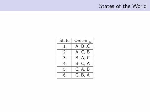
States of the World

State Ordering1 A, B ,C2 A, C, B3 B, A, C4 B, C, A5 C, A, B6 C, B, A

Acts

• This is what we mean by the states of the world• An exclusive and exhaustive list of all the possible outcomes ina scenario

• An act is then an action which is defined by the oucome itgives in each state of the world

• Here are two examples• Act f : A $10 even money bet that Archibald will win• Act g : A $10 bet at odds of 2 to 1 that Cumberbach will win

Acts

State Ordering Payoff Act f Payoff Act g1 A, B ,C $10 -$102 A, C, B $10 -$103 B, A, C -$10 -$104 B, C, A -$10 -$105 C, A, B -$10 $206 C, B, A -$10 $20

Subjective Expected Utility Theory

• So, how would you choose between acts f and g?• SEU assumes the following:

1 Figure out the probability you would associate with each stateof the world

2 Figure out the utility you would gain from each prize

3 Figure out the expected utility of each act according to thoseprobabilities and utilities

4 Choose the act with the highest utility


• So, in the above example• Utility from f :

[π(ABC ) + π(ACB)] u(10)

+ [π(BAC ) + π(BCA)] u(−10)+ [π(CBA) + π(CAB)] u(−10)

where π is the probability of each act

• Utility from g :

[π(ABC ) + π(ACB)] u(−10)+ [π(BAC ) + π(BCA)] u(−10)+ [π(CBA) + π(CAB)] u(20)


• Assuming utility is linear f is preferred to g if

[π(ABC ) + π(ACB)][π(CBA) + π(CAB)]

≥ 32

• Or the probability of A winning is more than 3/2 times theprobability of C winning


DefinitionLet X be a set of prizes, Ω be a (finite) set of states of the worldand F be the resulting set of acts (i.e. F is the set of all functionsf : Ω→ X ). We say that preferences on the set of acts F has asubjective expected utility representation if there exists a utilityfunction u : X → R and probability function π : Ω→ [0, 1] suchthat ∑ω∈Ω π(ω) = 1 and

f g

⇔ ∑ω∈Ω

π(ω)u (f (ω)) ≥ ∑ω∈Ω

π(ω)u (g(ω))

Notice that we now have two things to recover: Utility andpreferences


• As with expected utility theory, we would like a set of axiomson which are necessary and suffi cient for an SEUrepresentation

• Savage did this in 1954• In this setting it is pretty tricky• Why?

• Because really we still want to impose linearity in probabilities• Would like to impose something like the independence axiom• But we don’t know how to mix acts together

The Anscombe Aumann Set Up

• Anscombe and Aumann came up with a nice trick to getround this in 1963

• Rather than have acts pay off prizes in each state, have thempay off lotteries

• Let• X be a (finite) prize space• Ω be a finite state space

DefinitionAn Anscombe-Aumann act is a function h : Ω→ 4(X ). Let Hdefine the set of all such acts


• In this world we can define mixing

DefinitionThe mixture of two acts h, g ∈ H, αh+ (1− α)g ∈ H is the actsuch that, for each state ω ∈ Ω

(αh+ (1− α)g) (ω) = αh(ω) + (1− α)g(ω)


• And so define equivalents of the independence and continuityaxioms

The Independence Axiom h g implies that, for any other act fand number 0 < α ≤ 1 then

αh+ (1− α)f αg + (1− α)f

The Continuity Axiom For all acts h, g and f such thath g f , there must exist an a and b in (0, 1)such that

ah+ (1− a)f g bh+ (1− b)f


• If we add to this three standard axioms• is a preference relation• non degenerate• Monotonicity: if h(ω) g(ω) ∀ ω ∈ Ω then h g

• Then we get a modified SEU representation

DefinitionA preference relation on H has an SEU represenation if thereexists a utility function u : X → R and probability functionπ : Ω→ [0, 1] such that

h g

⇔ ∑ω∈Ω

π(ω)

[∑x∈X

h(ω)(x)u(x)

]≥ ∑

ω∈Ωπ(ω)

[∑x∈X

g(ω)(x)u(x)

]

The Ellsberg Paradox

• Unfortunately, while simple and intuitive, SEU theory hassome problems when it comes to describing behavior

• These problems are most elegantly demostrated by theEllsberg paradox

• This thought experiment has sparked a whole field of decisiontheory

The Ellsberg Paradox - A Reminder

• Choice 1: The ’risky bag’• Fill a bag with 20 red and 20 black tokens• Offer your subject the opportunity to place a $10 bet on thecolor of their choice

• Then elicit the amount x such that the subject is indifferentbetween playing the gamble and receiving $x for sure.

• Choice 2: The ‘ambiguous bag’• Repeat the above experiment, but provide the subject with noinformation about the number of red and black tokens

• Then elicit the amount y such that the subject is indifferentbetween playing the gamble and receiving $y for sure.


• Typical finding• x >> y• People much prefer to bet on the risky bag

• This behavior cannot be explained by SEU?• Why?


• What is the utility of betting on the risky bag?• The probability of drawing a red ball is the same as theprobability of drawing a black ball at 0.5

• So whichever act you choose to bet on, the utility of thegamble is

0.5u($10)


• What is the utility of betting on the ambiguous bag?• Here we need to apply SEU• What are the states of the world?

• Red ball is drawn or black ball is drawn

• What are the acts?• Bet on red or bet on black


State r bred 10 0black 0 10

• How do we calculate the utility of these two acts?• Need to decide how likely each state is• Assign probabilities π(r) = 1− π(b)• Note that these do not have to be 50%• Maybe you think I like red chips!


• Utility of betting on the red outcome is therefore

π(r)u($10)

• Utility of betting on the black outcome is

π(b)u($10) = (1− π(r))u($10)

• Because you get to choose which color to bet on, the gambleon the ambiguous urn is

max π(r)u($10), (1− π(r))u($10)

• is equal to 0.5u($10) if π(r) = 0.5• otherwise is greater than 0.5u($10)• should always (weakly) prefer to bet on the ambiguous urn• intuition: if you can choose what to bet on, 0.5 is the worstprobability


• 61% of my last class exhibited the Ellsberg paradox

• For more details see Halevy, Yoram. "Ellsberg revisited: Anexperimental study." Econometrica 75.2 (2007): 503-536.

Maxmin Expected Utility

• So, as usual, we are left needing a new model to explainbehavior

• There have been many such attempts since the Ellsbergparadox was first described

• We will focus on ’Maxmin Expected Utility’by Gilboa andSchmeidler1

1Gilboa, Itzhak & Schmeidler, David, 1989. "Maxmin expected utility withnon-unique prior," Journal of Mathematical Economics, Elsevier, vol. 18(2),pages 141-153, April.


• Maxmin expected utility has a very natural interpretation....• The world is out to get you!

• Imagine that in the Ellsberg experiment was run by an evil andsneaky experimenter

• After you have chosen whether to bet on red or black, they willincrease your chances of losing

• They will sneak some chips into the bag of the opposite colorto the one you bet on

• So if you bet on red they will put black chips in and visa versa


• How should we think about this?• Rather than their being a single probability distribution, thereis a range of possible distributions

• After you chose your act, you evaluate it using the worst ofthese distributions

• This is maxmin expected utility• you maximize the minimum utility that you can get acrossdifferent probability distributions

• Has links to robust control theory in engineering• This is basically how you design aircraft


DefinitionLet X be a set of prizes, Ω be a (finite) set of states of the worldand F be the resulting set of acts (i.e. F is the set of all functionsf : Ω→ X ). We say that preferences on the set of acts F has aMaxmin expected utility representation if there exists a utilityfunction u : X → R and convex set of probability functions Π and

f g

⇔ minπ∈Π

∑ω∈Ω

π(ω)u (f (ω)) ≥ minπ∈Π

∑ω∈Ω

π(ω)u (g(ω))


• Maxmin expected utility can explain the Ellsberg paradox• Assume that u(x) = x• Assume that you think π(r) is between 0.25 and 0.75• Utility of betting on the risky bag is 0.5u(x) = 5• What is the utility of betting on red from the ambiguous bag?

minπ(r )∈[0.25,0.75]

π(r)u($10) = 0.25u($10) = 2.5

• Similary, the utility from betting on black is

minπ(r )∈[0.25,0.75]

(1− π(r)) u($10) = 0.25u($10) = 2.5

• Maximal utility from betting on the ambiguous bag is lowerthan that from the risky bag

Risk and Uncertainty 2 - Columbia University

Documents

Transcript of Risk and Uncertainty 2 - Columbia University