Rigorous column simulation - SCDS - Chemstations · PDF filefocused on process simulation Page...
16
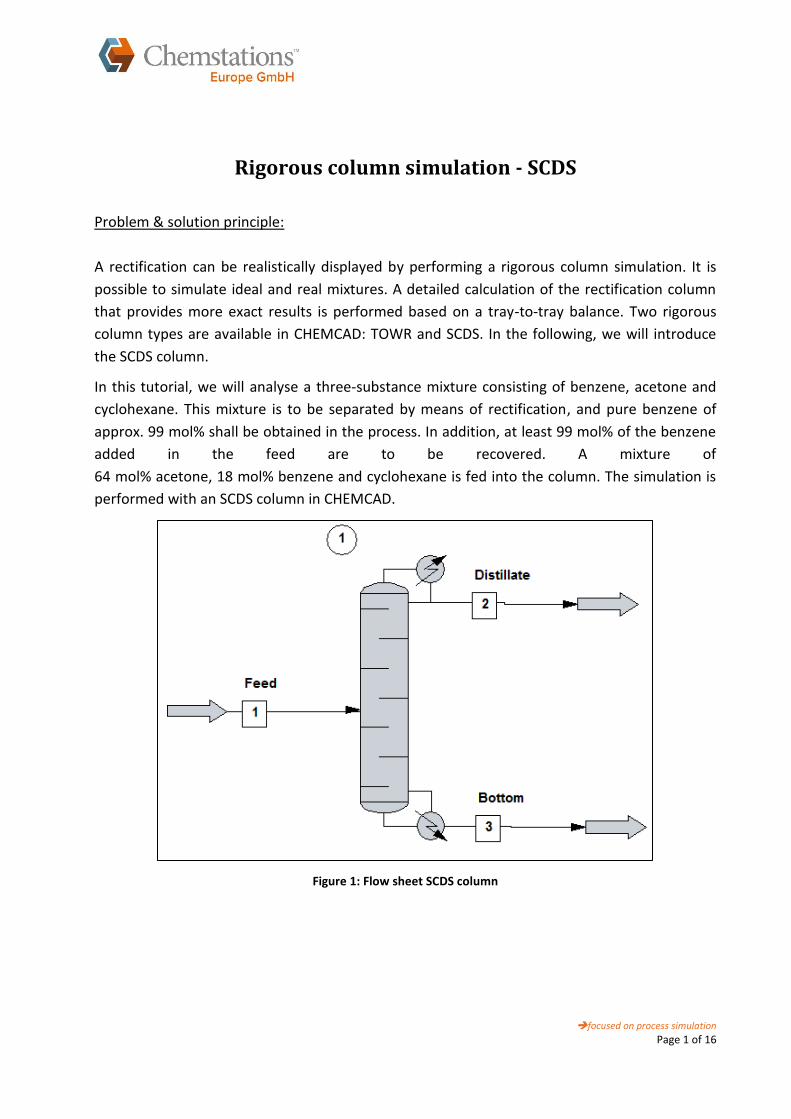
focused on process simulation Page 1 of 16 Rigorous column simulation - SCDS Problem & solution principle: A rectification can be realistically displayed by performing a rigorous column simulation. It is possible to simulate ideal and real mixtures. A detailed calculation of the rectification column that provides more exact results is performed based on a tray-to-tray balance. Two rigorous column types are available in CHEMCAD: TOWR and SCDS. In the following, we will introduce the SCDS column. In this tutorial, we will analyse a three-substance mixture consisting of benzene, acetone and cyclohexane. This mixture is to be separated by means of rectification, and pure benzene of approx. 99 mol% shall be obtained in the process. In addition, at least 99 mol% of the benzene added in the feed are to be recovered. A mixture of 64 mol% acetone, 18 mol% benzene and cyclohexane is fed into the column. The simulation is performed with an SCDS column in CHEMCAD. Figure 1: Flow sheet SCDS column
Transcript of Rigorous column simulation - SCDS - Chemstations · PDF filefocused on process simulation Page...
focused on process simulation
Page 1 of 16
Rigorous column simulation - SCDS
Problem & solution principle:
A rectification can be realistically displayed by performing a rigorous column simulation. It is
possible to simulate ideal and real mixtures. A detailed calculation of the rectification column
that provides more exact results is performed based on a tray-to-tray balance. Two rigorous
column types are available in CHEMCAD: TOWR and SCDS. In the following, we will introduce
the SCDS column.
In this tutorial, we will analyse a three-substance mixture consisting of benzene, acetone and
cyclohexane. This mixture is to be separated by means of rectification, and pure benzene of
approx. 99 mol% shall be obtained in the process. In addition, at least 99 mol% of the benzene
added in the feed are to be recovered. A mixture of
64 mol% acetone, 18 mol% benzene and cyclohexane is fed into the column. The simulation is
performed with an SCDS column in CHEMCAD.
Figure 1: Flow sheet SCDS column
focused on process simulation
Page 2 of 16
Implementation of the SCDS simulation in CHEMCAD
The simulation is performed with CHEMCAD Steady State. Prior to the simulation, the
components and the thermodynamic model must be selected. At "Thermophysical: Select
Components", the components benzene (CAS no.: 71-43-2), acetone (CAS no.: 67-64-1) and
cyclohexane (CAS no.: 110-82-7) are selected. The subsequent "Thermodynamics Wizard"
suggests a suitable model after specification of the pressure and the temperature. For the given
example, CHEMCAD recommends the k-value model NRTL. For the enthalpy model, LATE
(latent heat) is suggested. This selection is a preselection made by the program, and should
always be verified by the user or synchronised with a decision diagram ([3], figure 8/9).
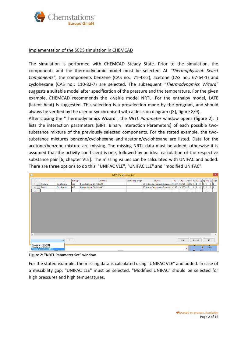
After closing the "Thermodynamics Wizard", the NRTL Parameter window opens (figure 2). It
lists the interaction parameters (BIPs: Binary Interaction Parameters) of each possible two-
substance mixture of the previously selected components. For the stated example, the two-
substance mixtures benzene/cyclohexane and acetone/cyclohexane are listed. Data for the
acetone/benzene mixture are missing. The missing NRTL data must be added; otherwise it is
assumed that the activity coefficient is one, followed by an ideal calculation of the respective
substance pair [6, chapter VLE]. The missing values can be calculated with UNIFAC and added.
There are three options to do this: "UNIFAC VLE", "UNIFAC LLE" and "modified UNIFAC".
Figure 2: "NRTL Parameter Set" window
For the stated example, the missing data is calculated using "UNIFAC VLE" and added. In case of
a miscibility gap, "UNIFAC LLE" must be selected. "Modified UNIFAC" should be selected for
high pressures and high temperatures.
focused on process simulation
Page 3 of 16
Prior to each simulation, the behaviour of the mixture must be examined in more detail to
determine possible rectification limitations (example: azeotrope, distillation limitations,
miscibility gaps). To detect miscibility gaps, the equilibrium diagram should be checked first for
each binary substance mixture at "Plot: TPXY". We can see that there is no miscibility gap. A
rough estimation concerning miscibility can also be made via the molecular structure. However,
if there is a miscibility gap, the vapour-liquid-liquid equilibrium must be selected at Global
Phase Option (Thermodynamic Settings, option: Vapor/Liquid/Liquid/Solid).
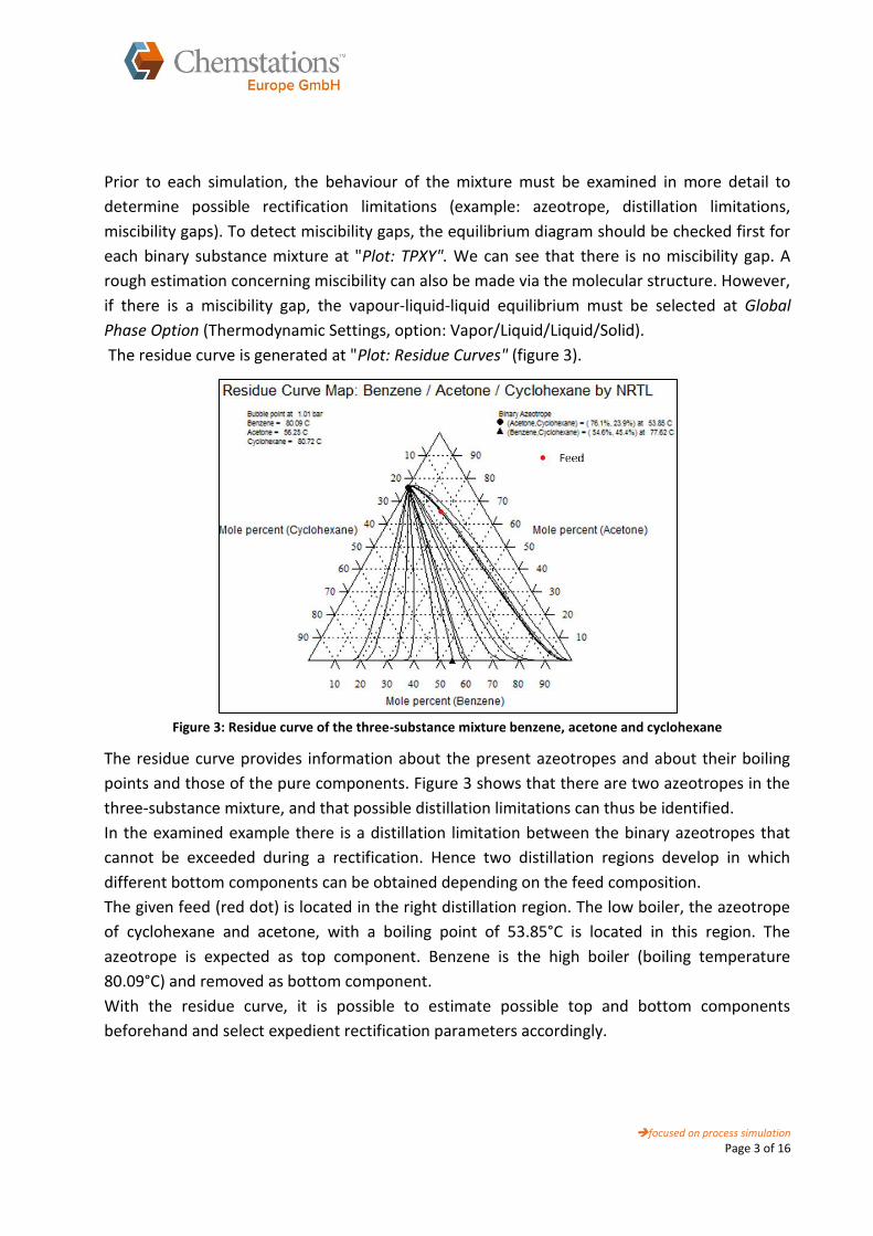
The residue curve is generated at "Plot: Residue Curves" (figure 3).
Figure 3: Residue curve of the three-substance mixture benzene, acetone and cyclohexane
The residue curve provides information about the present azeotropes and about their boiling
points and those of the pure components. Figure 3 shows that there are two azeotropes in the
three-substance mixture, and that possible distillation limitations can thus be identified.
In the examined example there is a distillation limitation between the binary azeotropes that
cannot be exceeded during a rectification. Hence two distillation regions develop in which
different bottom components can be obtained depending on the feed composition.
The given feed (red dot) is located in the right distillation region. The low boiler, the azeotrope
of cyclohexane and acetone, with a boiling point of 53.85°C is located in this region. The
azeotrope is expected as top component. Benzene is the high boiler (boiling temperature
80.09°C) and removed as bottom component.
With the residue curve, it is possible to estimate possible top and bottom components
beforehand and select expedient rectification parameters accordingly.

focused on process simulation
Page 4 of 16
Table 1: Data of relevance for the simulation
Units Components Thermo-
dynamics
Feed
streams
Unit operations
SI Benzene
Acetone
Cyclohexane
K: NRTL, H: LATE
1 SCDS column
1 feed stream
2 product
streams
The UnitOp (unit operation) of the SCDS column is entered in the flow sheet and allocated a
feed stream and two product streams. The feed stream is set to liquid boiling with the data
stated in table 1 (see figure 4).
Figure 4: Feed settings window
focused on process simulation
Page 5 of 16
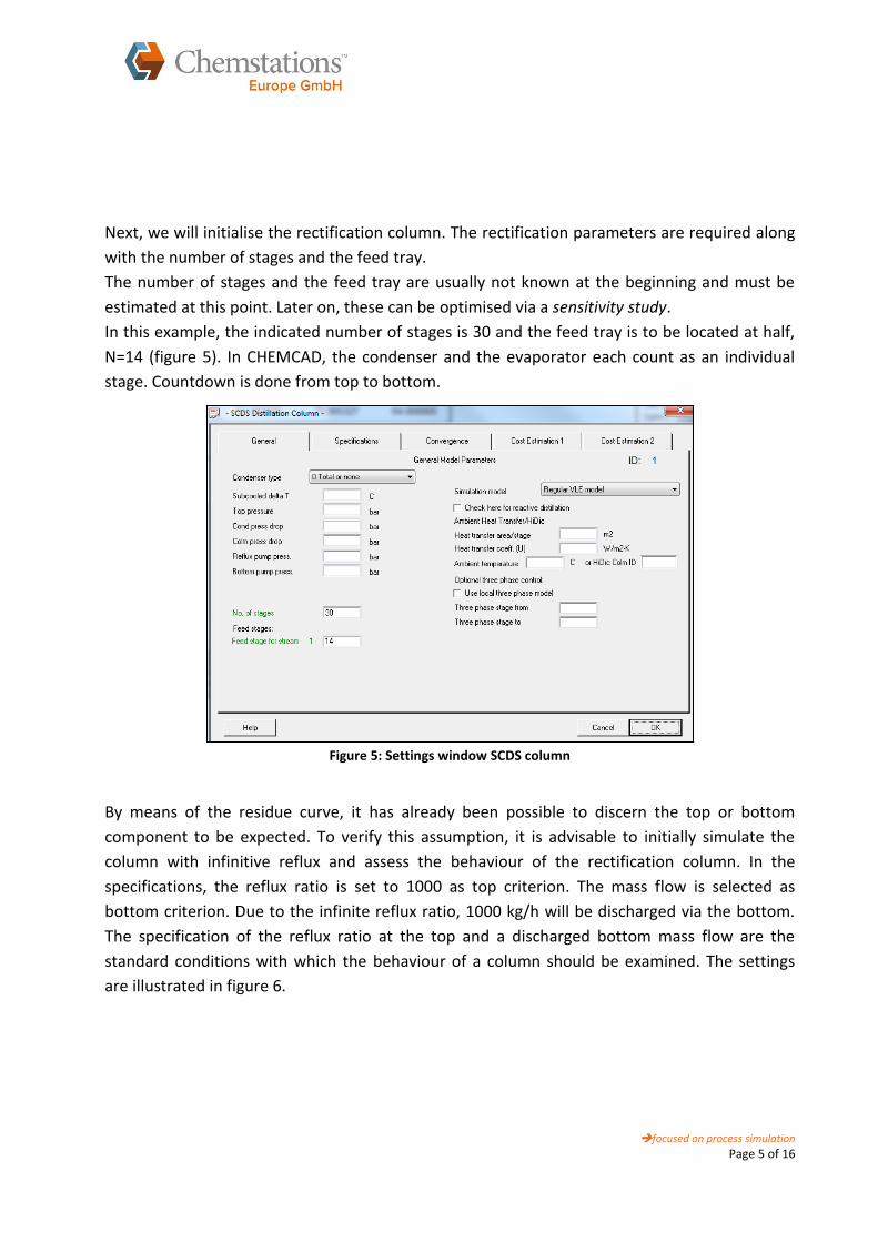
Next, we will initialise the rectification column. The rectification parameters are required along
with the number of stages and the feed tray.
The number of stages and the feed tray are usually not known at the beginning and must be
estimated at this point. Later on, these can be optimised via a sensitivity study.
In this example, the indicated number of stages is 30 and the feed tray is to be located at half,
N=14 (figure 5). In CHEMCAD, the condenser and the evaporator each count as an individual
stage. Countdown is done from top to bottom.
Figure 5: Settings window SCDS column
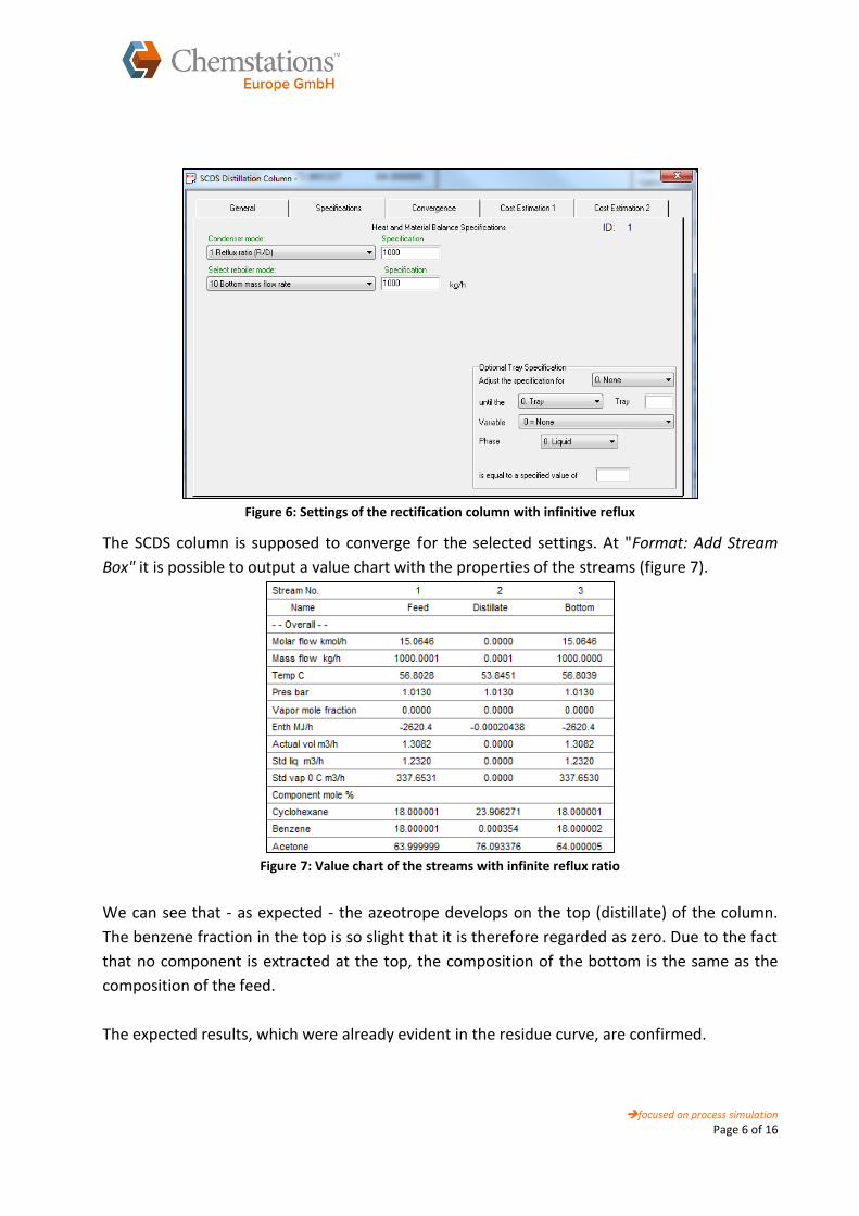
By means of the residue curve, it has already been possible to discern the top or bottom
component to be expected. To verify this assumption, it is advisable to initially simulate the
column with infinitive reflux and assess the behaviour of the rectification column. In the
specifications, the reflux ratio is set to 1000 as top criterion. The mass flow is selected as
bottom criterion. Due to the infinite reflux ratio, 1000 kg/h will be discharged via the bottom.
The specification of the reflux ratio at the top and a discharged bottom mass flow are the
standard conditions with which the behaviour of a column should be examined. The settings
are illustrated in figure 6.
focused on process simulation
Page 6 of 16
Figure 6: Settings of the rectification column with infinitive reflux
The SCDS column is supposed to converge for the selected settings. At "Format: Add Stream
Box" it is possible to output a value chart with the properties of the streams (figure 7).
Figure 7: Value chart of the streams with infinite reflux ratio
We can see that - as expected - the azeotrope develops on the top (distillate) of the column.
The benzene fraction in the top is so slight that it is therefore regarded as zero. Due to the fact
that no component is extracted at the top, the composition of the bottom is the same as the
composition of the feed.
The expected results, which were already evident in the residue curve, are confirmed.
focused on process simulation
Page 7 of 16
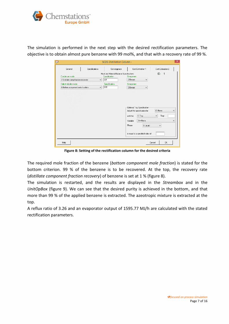
The simulation is performed in the next step with the desired rectification parameters. The
objective is to obtain almost pure benzene with 99 mol%, and that with a recovery rate of 99 %.
Figure 8: Setting of the rectification column for the desired criteria
The required mole fraction of the benzene (bottom component mole fraction) is stated for the
bottom criterion. 99 % of the benzene is to be recovered. At the top, the recovery rate
(distillate component fraction recovery) of benzene is set at 1 % (figure 8).
The simulation is restarted, and the results are displayed in the Streambox and in the
UnitOpBox (figure 9). We can see that the desired purity is achieved in the bottom, and that
more than 99 % of the applied benzene is extracted. The azeotropic mixture is extracted at the
top.
A reflux ratio of 3.26 and an evaporator output of 1595.77 MJ/h are calculated with the stated
rectification parameters.

focused on process simulation
Page 8 of 16
Figure 9: Properties of the streams and column after the simulation
The number of stages and the feed tray were estimated at the start. Now the optimum number
of stages and the optimum feed tray can be determined with a sensitivity study.
To determine the optimum number of stages, the evaporator output is applied across the
number of stages and examined for a minimum.
The number of stages is varied from 5 to 50 and the evaporator output calculated for each
stage in the process (figure 10).
focused on process simulation
Page 9 of 16
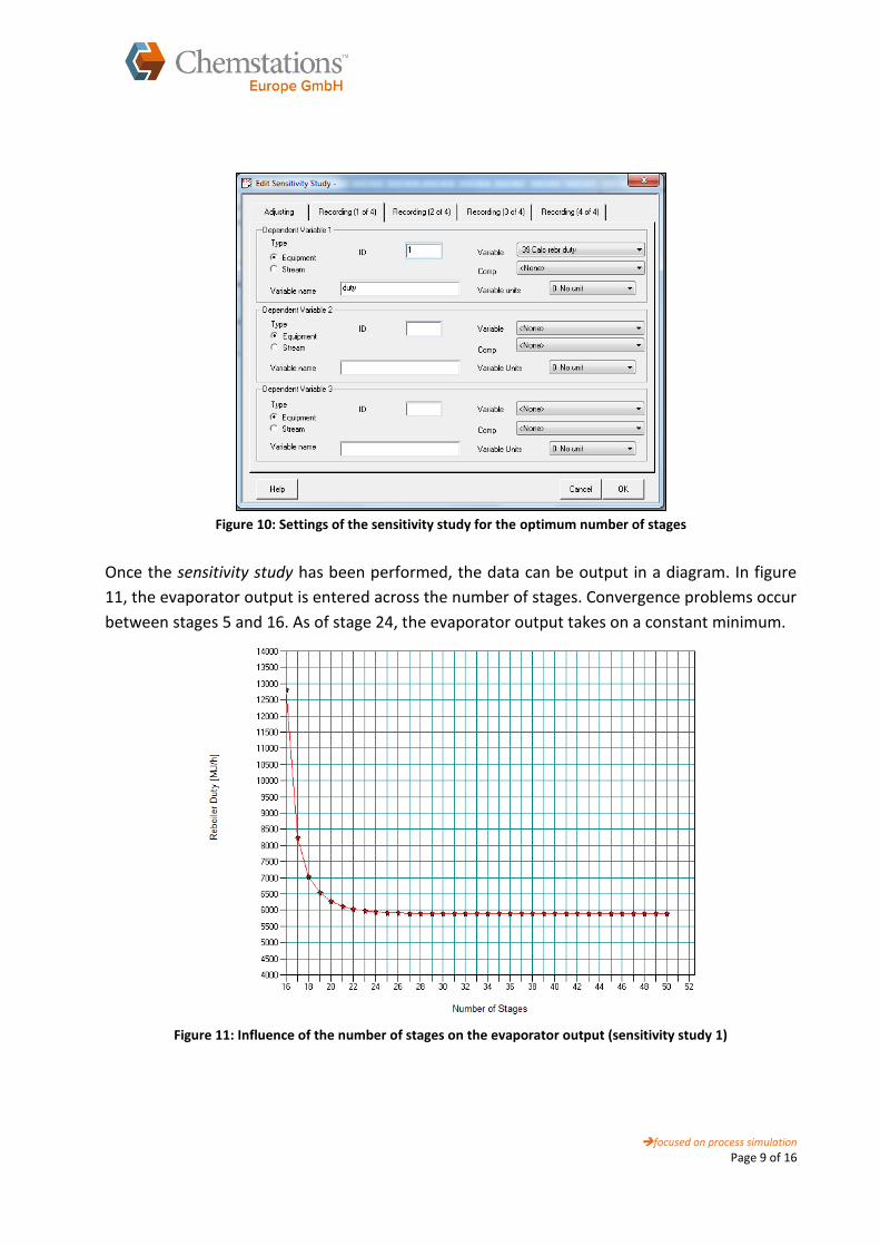
Figure 10: Settings of the sensitivity study for the optimum number of stages
Once the sensitivity study has been performed, the data can be output in a diagram. In figure
11, the evaporator output is entered across the number of stages. Convergence problems occur
between stages 5 and 16. As of stage 24, the evaporator output takes on a constant minimum.
Figure 11: Influence of the number of stages on the evaporator output (sensitivity study 1)

focused on process simulation
Page 10 of 16
In the column properties, the number of stages is changed to 24 and the simulation is restarted.
Next, the optimum feed tray is defined. A second sensitivity study is performed for this
purpose. The feed tray is varied across the column height, and in doing so the influence on the
reflux ratio is analysed. The feed tray that is varied from stage 4 to stage 20 is used as variable.
The reflux ratio calculated for each stage is set as dependent variable. The correlation is
illustrated in figure 12.
Figure 12: Influence of the feed position on the reflux ratio
We can see that the reflux ratio takes on a minimum around stage number 10. The lower the
reflux ratio, the lower also the energy consumption of the column. For this reason, the feed is
supplied at stage 10.
The column settings are adapted again, and the simulation is started.
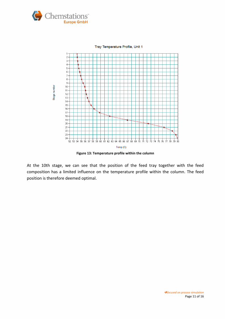
It is advisable to check to what extent the feed position influences the equilibrium position
within the column. The temperature profile across the stages can be generated at "Plot: UnitOp
Plots: Column Profiles" (figure 13).
focused on process simulation
Page 11 of 16
Figure 13: Temperature profile within the column
At the 10th stage, we can see that the position of the feed tray together with the feed
composition has a limited influence on the temperature profile within the column. The feed
position is therefore deemed optimal.

focused on process simulation
Page 12 of 16
The procedure for initialising a rigorous rectification column (SCDS column) is summarised once
again in table 2.
Table 2: Summary "Simulation of an SCDS column"
Procedures Benefits/information
- Select components & thermodynamic
model
[Thermophysical [Select Components] &
[Thermodynamics Wizard]
- Setting of the calculation bases
- Selection of the thermodynamic model has a
pronounced influence on the calculation
- Plotting of the residue curve
[Plot] [Residue Curve]
- Identification of possible azeotropes and
distillation limitations
- Definition of the top and bottom component
to be expected
- Creating the flow sheet
- Assumption: Number of stages and feed tray
- Setting of an infinite
reflux ratio and complete extraction via
the bottom
- Analysis of the column behaviour
- Determination of the top concentration
to be expected
- Setting of the rectification parameters
- If the rectification parameter is
e.g. an azeotrope, successive
approximation is expedient
- At Convergence in the settings window
of the column, the option Reload
Column Profile can be used to facilitate
successive approximation
- Optimising the number of stages by means
of a
sensitivity study
[Run] [Sensitivity]
- Optimising the number of stages by
determining the correlation between
evaporator output and number of stages
- Economically optimal number of stages with
minimum evaporator output
- Determination of the feed tray by means of
a
sensitivity study
[Run] [Sensitivity]
- Determination of the feed tray position
by determining the correlation
between reflux ratio and feed tray
- Economically optimal feed tray with
minimum reflux ratio

focused on process simulation
Page 13 of 16
Rating
The properties of the streams and the column are shown at "Format: Add Stream Box und Add
UnitOp Box“ (figure 14).
We can see that the azeotrope consisting of cyclohexane and acetone is separated at the top of
the column. Benzene is only extracted in very slight quantities. Almost pure benzene is
obtained at the bottom.
The results show that it has been possible to reduce the evaporator output to 1355.03 MJ/h. It
has also been possible to reduce the reflux ratio to 2.58.
Figure 14: Results after simulation of the rigorous column
focused on process simulation
Page 14 of 16
Fundamental principles
This tutorial investigates the simulation of the rigorous column SCDS. No simplifications are
made in the calculation of rigorous columns, which is otherwise the case with the shortcut
method. Each tray is balanced individually, which results in a complex equation system that
must be solved by means of numerical algorithms. The rigorous column simulation is
mathematically more extensive in comparison to the shortcut method, but provides much
more exact and realistic results.
Ideal mixtures can be quickly displayed as rough estimates with the shortcut column. The
problem is, however, that it cannot be used for non-ideal mixtures, like for example azeotropic
mixtures, because it no longer reflects realistic conditions due to the pronounced
simplifications in the calculation. For this reason, rigorous column simulation is used for non-
ideal mixtures.
The SCDS column is one of the rigorous columns that can be used in CHEMCAD. SCDS stands for
"Simultaneous Correction Distillation System". It is a very versatile column model that is suited
for all rectification processes.
When calculating the rigorous SCDS column, a stationary state between liquid-vapour phase or
liquid-liquid phase is assumed for each tray. The following assumptions are made:
1) Each tray is defined as a thermodynamic system in which the phase equilibrium is
reached.
2) No chemical reactions occur.
3) The uptake of liquid drops in the gas phase and the inclusion of gas bubbles in the liquid
phase are not considered.
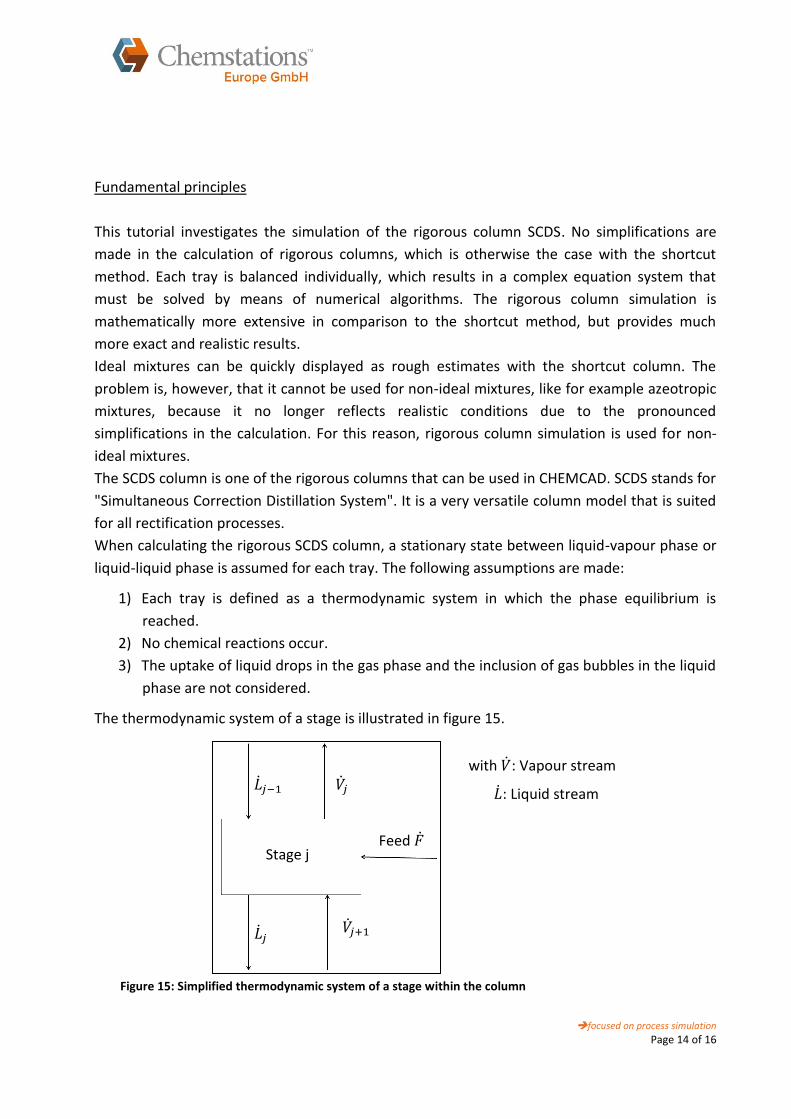
The thermodynamic system of a stage is illustrated in figure 15.
Feed
with : Vapour stream
: Liquid stream
Figure 15: Simplified thermodynamic system of a stage within the column
Stage j

focused on process simulation
Page 15 of 16
For this thermodynamic system, the required equilibrium equations of relevance for the design
are summarised using the MESH method. MESH stands for Material balance, Equilibrium,
Summation condition and Heat balance.
This way, a complex equation system results for each tray. The mathematical calculation is very
extensive and convergence algorithms are required to solve it. The respective literature states a
large number of iterative solution approaches for solving these non-linear algebraic equation
systems.
General solution algorithms that do not have any restrictions and are applicable for all cases are
the simultaneous correction method and the inside-out method. They can be used for all
column types and all feed compositions. Both algorithms are used in CHEMCAD.
With the simultaneous correction method (SC), all MESH equations as well as their
combinations are solved simultaneously with the help of the iterative Newton-Raphson
method.
Further application options of SCDS are:
Column simulation with packing
Column simulation with special trays
Adsorption and/or absorption processes
focused on process simulation
Page 16 of 16
The above simulation was generated in CHEMCAD 6.4.0.
Are you interested in further tutorials, seminars or other solutions with CHEMCAD?
Then please visit our website.
www.chemstations.eu
Or please contact us.
Mail: [email protected]
Phone: +49 (0)30 20 200 600
www.chemstations.eu
Authors:
Lisa Weise
Sources:
[1] Kister, Henry Z.: Distillation design. McGraw-Hill, 1992
[2] Gmehling, Jürgen: Kolbe, Bärbel: Kleiber, Michael: Rarey, Jürgen: Chemical Thermodynamics
for Process Simulation. Wiley-VCH Verlag, 2012
[3] Edwards, John: Process Modeling Selection of Thermodynamic Methods
[4] Schmidt, Wolfgang: USER NRTL BIPS, 2011
[5] Sattler, Klaus: Thermische Trennverfahren: Grundlagen, Auslegung, Apparate. Wiley-VCH
Verlag, pp. 199-202
[6] CHEMCAD help
[7] Seader; Siirola; Barnicki: Perry's Chemical Engineers' Handbook, Section 13 Distillation, 7th
edition. McGraw-Hill, New York, (1997)
[8] Kontogeorgis, Folas: Thermodynamic Models for Industrial Applications, Wiley-VCH Verlag,
2010