No-Reference Noise and Blur Detection via the Fourier Transform

Richard W. Dosselmann and Xue Dong Yang

Technical Report CS-2012-01August 2012

Copyright c© 2012, R.W. Dosselmann and X.D. YangDepartment of Computer Science

University of ReginaRegina, SK, CANADA

S4S 0A2

ISSN 0828-3494ISBN 978-0-7731-0714-4 (on-line)

No-Reference Noise and Blur Detection via the FourierTransform

Richard Dosselmann and Xue Dong YangDepartment of Computer Science, University of Regina

3737 Wascana Parkway, Regina, Saskatchewan, Canada S4S 0A2{dosselmr, yang}@cs.uregina.ca

Abstract

This research presents a new method of distinguishing between noisy, blurred and oth-erwise uncorrupted images via the Fourier transform. The spectrum of an image corruptedby noise is markedly different from one that is marred by blurring, or one that is not dam-aged at all. In particular, there are more high frequency terms in the spectrum of a noisyimage than in that of a blurred image, and, to a lesser degree, that of an image that has notbeen altered. So as to better emphasize these distinctions, a cumulative distribution func-tion of the terms of the spectrum of an image is assembled. Using only this construct, a newtechnique that enables a machine to reliably assess the number of high frequency terms inan image, and therefore differentiate among the three types of images, is brought forward.

Keywords: noise, blur, Fourier transform, cumulative distribution function, image quality met-ric

1 Introduction

Images [1] are frequently disrupted by noise [2]. This distortion may turn up as part of the ini-tial acquisition stage, or later, perhaps during transmission. Among the most common types ofnoise are the uniform [1], or, in this work, random, Gaussian [1] and salt-and-pepper [1] vari-eties. Blurring [3] is another troublesome issue. Failing to properly focus a camera, for example,may bring about this error. Most prominent are those stemming from averaging filters [1], or,here, an averaging blur, as well as Gaussian [2] and motion [1] blurs. The goal of this research isto automatically identify those images that are noisy or blurred, as well as those in which neithererror occurs. The strategy proposed by this research is based on the classic Fourier transform[1] (FT) and the realization that a noisy image, transformed to the frequency domain [1], con-tains far more high frequency [4] terms than does a blurred image. The primary applications ofthis work are in the area of image quality [2] assessment. Existing image quality metrics [5] gen-erally work by comparing an image with its “original” or “perfect” form. The routine absenceof an original image greatly limits the utility of these full-reference [6] (FR) metrics. While thetechnique presented in this work is also tested in an FR framework, it is principally designed

1

to be a no-reference [6] (NR) metric, meaning that it functions without any original image. Itis therefore ideally suited for real-world applications, such as monitoring television and videocontent or spotting problems in images taken with a camera or cell phone. Before proceeding,note that the ideas outlined in this work were originally documented in [7, 8].

Traditionally, noise has been caught by comparing pixels in local image patches againstsome preset threshold. Those exceeding this threshold are surmised to be noise. Approaches inthis direction include those of [9, 10, 11]. This task is usually easier when more than one image isavailable, perhaps a sequence of video frames. In this context, any pixel that does not reappearin the frame following the current is deemed to be noise. This is the methodology employed in[12], working specifically with a series of x-rays images. Smolka [13], drawing on the ideas ofothers [14], measures distances between pixels in a multidimensional space. Complementingthese various methods are several based on techniques of machine learning [15]. Saradhadeviand Sundaram [16], as an example, train a neural network [17] to spot potential noise pixels. Inanother instance, Zhang and Wang [18] distinguish between pixels belonging to an image andthose that are likely noise using fuzzy logic [19]. Blurring pares down and warps edges [1]. Thelogical response is therefore to examine the strength of the edges in an image, just as is donein [20, 21, 22], for instance. In a related technique, Levin [23] unearths blurred regions of animage by examining histograms [24] of edges. Following a strategy independent of that given inthis work, Tolhurst et al. [25] explore the general makeup of images from the perspective of thefrequency domain. Liu, Li and Jia [26] also travel down this path, this time looking at the powerspectrum [1] of an image. Machine learning resurfaces in [27], this time in the form of supportvector machines [28] (SVM). Here, the authors train their system to recognize the histograms ofblurred images, an idea similar in spirit to that of Levin [23].

Following an overview of the new technique in Section 2, the ideas introduced in this workare thoroughly tested in Section 3. Some concluding remarks are then given in Section 4.

2 Method

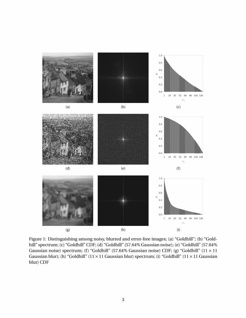
The intuition behind the method described in this paper is most easily explained by way of anexample. Take, then, the scenario depicted in Figure 1. An original image, along with its noisyand blurred counterparts, are given in Figures 1a, 1d and 1g, respectively. The correspondingFourier spectra [1] of these three images are shown in Figures 1b, 1e and 1h, respectively. Toallow for improved viewing, all three spectra have been scaled and brightened. The remainingillustrations, namely those of Figures 1c, 1f and 1i, are discussed at length in a moment. Onewill notice that the outer expanses of the spectrum of Figure 1b are fainter than those of thenoisy image, seen in Figure 1e, while it is more cluttered than the spectrum of the blurred pic-ture, given in Figure 1h. The random noise of Figure 1d produces sudden and steep changesin shading values across that image, leading to this increased concentration of high frequencyterms in the outer regions of the spectrum of Figure 1e. In an opposite fashion, the averagingblur of Figure 1g smoothes image content, resulting in fewer high frequency terms, just as isobserved in Figure 1h. The last case, namely the spectrum of Figure 1b, lies somewhere “in be-tween” these two. The number of high frequency terms in the outer portions of a spectrum isthe main focus of this research.

2

(a) (b)

0.0

0.2

0.4

0.6

0.8

1.0

1 18 35 52 69 86 103 120r i

p i

(c)

(d) (e)

0.0

0.2

0.4

0.6

0.8

1.0

1 18 35 52 69 86 103 120r i

p i

(f)

(g) (h)

0.0

0.2

0.4

0.6

0.8

1.0

1 18 35 52 69 86 103 120r i

p i

(i)

Figure 1: Distinguishing among noisy, blurred and error-free images; (a) “Goldhill”; (b) “Gold-hill” spectrum; (c) “Goldhill” CDF; (d) “Goldhill” (57.64% Gaussian noise); (e) “Goldhill” (57.64%Gaussian noise) spectrum; (f) “Goldhill” (57.64% Gaussian noise) CDF; (g) “Goldhill” (11× 11Gaussian blur); (h) “Goldhill” (11×11 Gaussian blur) spectrum; (i) “Goldhill” (11×11 Gaussianblur) CDF

3

2.1 Cumulative Distribution Function

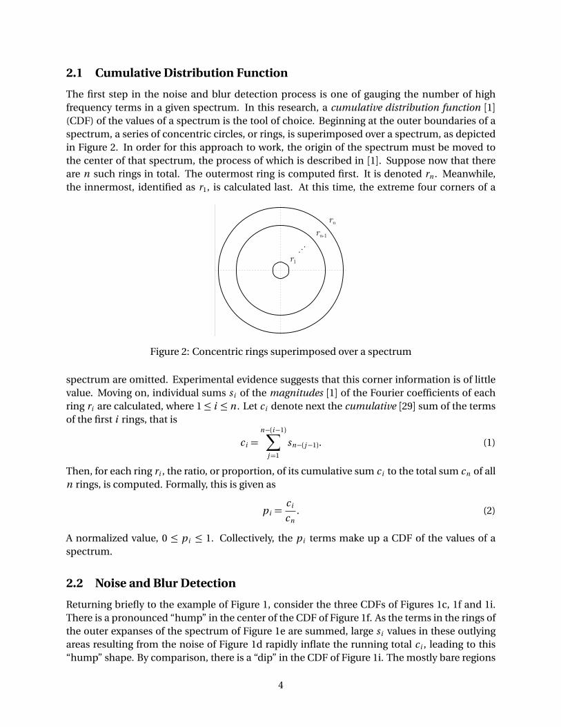
The first step in the noise and blur detection process is one of gauging the number of highfrequency terms in a given spectrum. In this research, a cumulative distribution function [1](CDF) of the values of a spectrum is the tool of choice. Beginning at the outer boundaries of aspectrum, a series of concentric circles, or rings, is superimposed over a spectrum, as depictedin Figure 2. In order for this approach to work, the origin of the spectrum must be moved tothe center of that spectrum, the process of which is described in [1]. Suppose now that thereare n such rings in total. The outermost ring is computed first. It is denoted rn . Meanwhile,the innermost, identified as r1, is calculated last. At this time, the extreme four corners of a

rn-1

r1·· ·

rn

Figure 2: Concentric rings superimposed over a spectrum

spectrum are omitted. Experimental evidence suggests that this corner information is of littlevalue. Moving on, individual sums s i of the magnitudes [1] of the Fourier coefficients of eachring ri are calculated, where 1≤ i ≤ n . Let c i denote next the cumulative [29] sum of the termsof the first i rings, that is

c i =n−(i−1)∑

j=1

sn−(j−1). (1)

Then, for each ring ri , the ratio, or proportion, of its cumulative sum c i to the total sum cn of alln rings, is computed. Formally, this is given as

p i =c i

cn. (2)

A normalized value, 0 ≤ p i ≤ 1. Collectively, the p i terms make up a CDF of the values of aspectrum.

2.2 Noise and Blur Detection

Returning briefly to the example of Figure 1, consider the three CDFs of Figures 1c, 1f and 1i.There is a pronounced “hump” in the center of the CDF of Figure 1f. As the terms in the rings ofthe outer expanses of the spectrum of Figure 1e are summed, large s i values in these outlyingareas resulting from the noise of Figure 1d rapidly inflate the running total c i , leading to this“hump” shape. By comparison, there is a “dip” in the CDF of Figure 1i. The mostly bare regions

4

at the ends of the spectrum of Figure 1h, a consequence of the blur of Figure 1g, initially holddown the value of c i , giving rise to a CDF that is depressed on the right side. The more orless “balanced” spectrum of Figure 1b yields a progressively increasing series of values, as isapparent from Figure 1c. This last CDF lies “in between” those of the noisy and blurred images.In some sense, images exist along a continuum, with those that are noisy or blurred positionedat opposite ends and the originals centered in between.

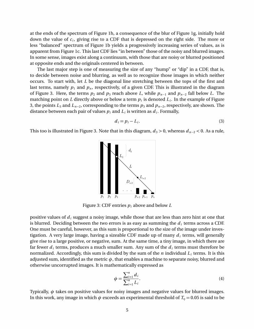
The last major step is one of measuring the size of any “hump” or “dip” in a CDF, that is,to decide between noise and blurring, as well as to recognize those images in which neitheroccurs. To start with, let L be the diagonal line stretching between the tops of the first andlast terms, namely p1 and pn , respectively, of a given CDF. This is illustrated in the diagramof Figure 3. Here, the terms p2 and p3 reach above L, while pn−1 and pn−2 fall below L. Thematching point on L directly above or below a term p i is denoted L i . In the example of Figure3, the points L 3 and L n−2, corresponding to the terms p3 and pn−2, respectively, are shown. Thedistance between each pair of values p i and L i is written as d i . Formally,

d i = p i − L i . (3)

This too is illustrated in Figure 3. Note that in this diagram, d 3 > 0, whereas d n−2 < 0. As a rule,

L

p1 p2 p3 pn-2 pn-1 pn. . .

Ln-2

L3

d3

Dn-2

Figure 3: CDF entries p i above and below L

positive values of d i suggest a noisy image, while those that are less than zero hint at one thatis blurred. Deciding between the two errors is as easy as summing the d i terms across a CDF.One must be careful, however, as this sum is proportional to the size of the image under inves-tigation. A very large image, having a sizeable CDF made up of many d i terms, will generallygive rise to a large positive, or negative, sum. At the same time, a tiny image, in which there arefar fewer d i terms, produces a much smaller sum. Any sum of the d i terms must therefore benormalized. Accordingly, this sum is divided by the sum of the n individual L i terms. It is thisadjusted sum, identified as the metricφ, that enables a machine to separate noisy, blurred andotherwise uncorrupted images. It is mathematically expressed as

φ =

∑ni=1 d i∑n

i=1 L i

. (4)

Typically, φ takes on positive values for noisy images and negative values for blurred images.In this work, any image in which φ exceeds an experimental threshold of Tη = 0.05 is said to be

5

“noisy”. “Blurring” occurs whenever φ < Tβ = −0.35. Lastly, an image is said to be “error-free”whenever Tβ ≤φ ≤ Tη.

As mentioned in the opening of Section 1, this metric can also be adapted to operate in afull-reference environment in which there is an original image that can be used as part of acomparison process. In this FR setting, the d i terms of a noisy image are normally larger thanthose of the original image. Similarly, these terms are smaller than those of the original in thecase of a blurred image. In response,φ is redefined for this full-reference case as

φ =

∑ni=1

�

d i −d ∗i�

∑ni=1 L i

, (5)

where d ∗i is the difference given by (3) for the original image, while d i is that of the given, andpossibly, corrupted image. A given image is found to be “noisy” if φ > 0. Likewise, an image is“blurred” ifφ < 0.

2.3 Noise and Blur Quantification

In its current form,φ is an indirect estimate of the quantity of noise or blurring in a given image.This metric generally assumes large positive values for very noisy images and small, frequentlynegative, values for those that are severely blurred. The relationship between φ and the levelof distortion is not, however, a direct one. This means, for instance, that two images, both cor-rupted by the same amount of random noise, may be assigned different values of φ. One ofthese two images might be highly detailed, while the other may be much less so. Consequently,the value of φ depends on the content of the particular image under scrutiny. This is an es-pecially exciting prospect. It essentially means that φ is a perceptual measure of quality ratherthan a trivial mathematical measure of quality. Other groups find their own names for thesetypes of measures, such as statistical measures [5] and visual front-end models [5], respectively.In the aforementioned example, the highly detailed image, which conceals noise, appears to beless noisy to a human observer than does the less cluttered image. It is therefore advantageousthat the new metric judges them as such. In short, φ, as presently computed, is a perceptualestimate of the level of noise or blurring in an image. This is validated using human-deriveddata in Section 3.2.

3 Experiments and Discussion

As a means of validating the ideas of Section 2, an experiment involving 80 uncorrupted images,each 256×256 in size, was carried out. These images were randomly selected from various sitesacross the Internet. Six corrupted versions of each of these 80 test images were syntheticallygenerated using random, Gaussian and salt-and-pepper noise, as well as averaging, Gaussianand motion blurring, respectively. In total, 80·6= 480 corrupted images were created. Together,with the 80 original images themselves, 480+ 80= 560 images were tested. Noise was injectedin random amounts ranging from 0.01% to 99.99%. The size of the averaging and Gaussian blurfilters [1] varied between 3× 3 and 65× 65. As for the motion blur, the direction was randomlychosen between 0◦ and 359◦, with a magnitude of between 1 and 32 pixels in length.

6

ErrorNumber of Number of Correctly Proportion of CorrectlyTest Images Classified Images Classified Images

none (error-free) 80 76 95.00%

random noise 80 76 95.00%Gaussian noise 80 66 82.50%

salt-and-pepper noise 80 79 98.75%total (noise) 240 221 92.08%

averaging blur 80 79 98.75%Gaussian blur 80 80 100.00%motion blur 80 66 82.50%total (blur) 240 225 93.75%

total 560 522 93.21%

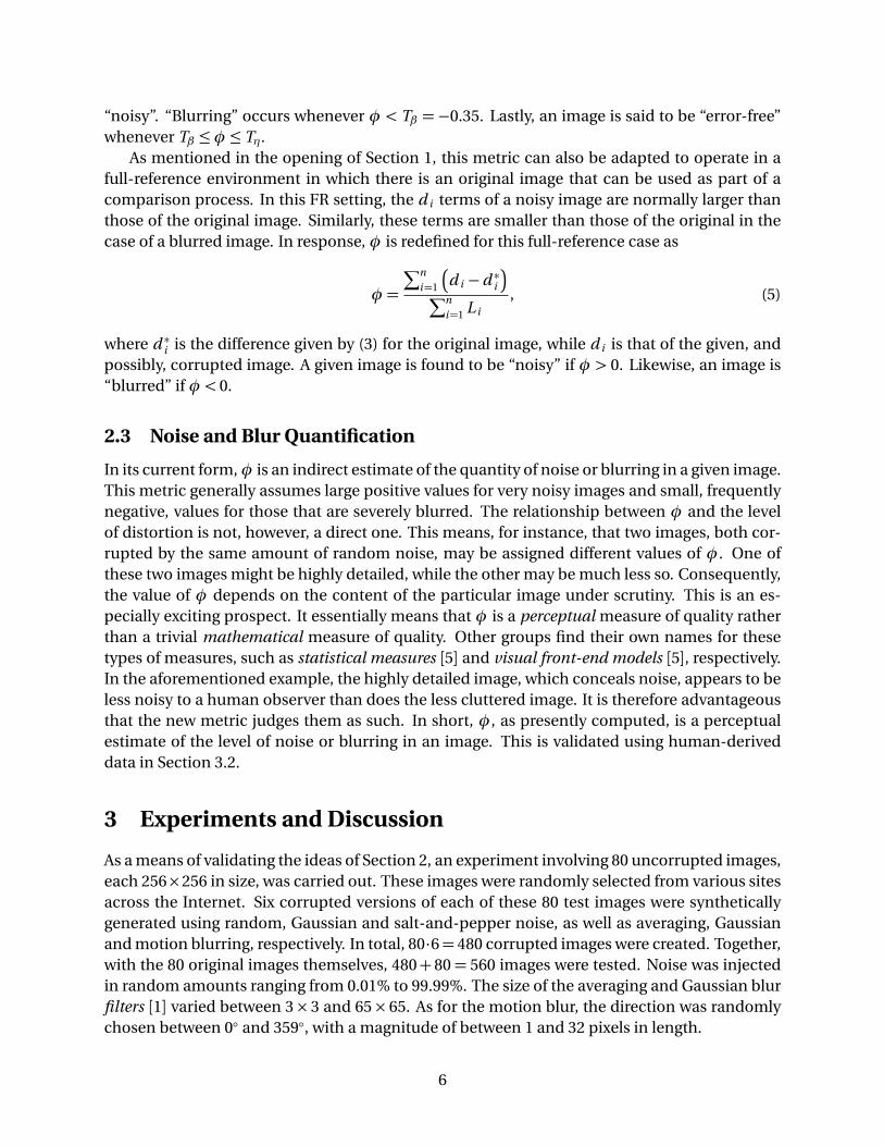
Table 1: Experimental results for no-reference noise, blur and error-free detection usingφ

3.1 Noise and Blur Detection

Each of the 560 test images was checked for noise, blur or the absence thereof by way of the newmetric φ of Section 2.2. The actual quantification of the level of noise or blur is explored laterin Section 3.2. Beginning first with the detection phase of this experiment,φ has proven to be adecidedly very effective metric. This is especially true when it comes to the full-reference case.In this case, only the 480 corrupted images, 80 · 3 = 240 noisy and 80 · 3 = 240 blurred, were, ofcourse, analyzed. With the original images in hand, all 240 noisy images were properly markedas being noisy. This represents a classification accuracy of 100%. Likewise, of the 240 blurredimages, all 240, or 100%, were labeled as such. This perfect classification is an indication of thestrength of the proposed method.

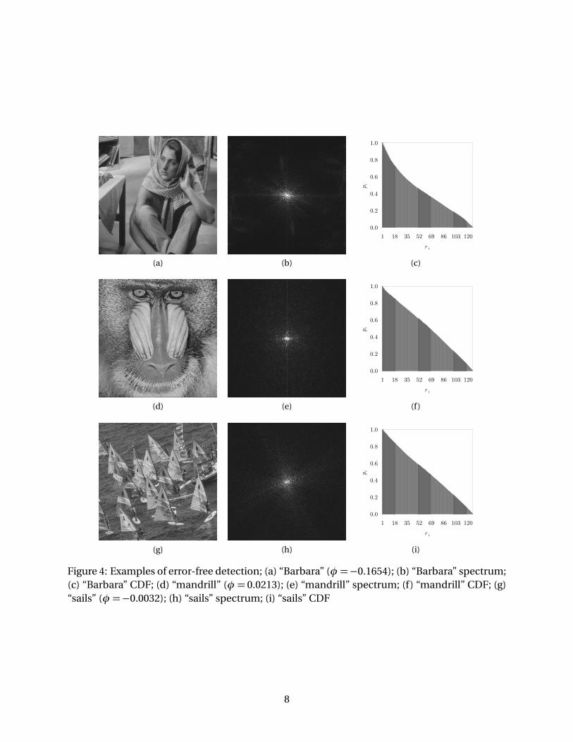
Excellent results were also obtained in the much more challenging no-reference case. Of the80 original images, 76, or 95.00%, were determined to be free of any errors. These results, alongwith those of the rest of this section, are organized in Table 1.

Three of these original images are seen in Figure 4. While there are certainly minor differ-ences between the three spectra, given in Figures 4b, 4e and 4h, respectively, the resulting CDFs,shown in Figures 4c, 4f and 4i, respectively, are remarkably similar. The slightly warped shapeof the CDF of Figure 4c does not significantly impact the resulting value of φ. With a value of−0.1654,φ properly falls between the thresholds of Tη and Tβ . Of particular interest is the pop-ular “mandrill” image of Figure 4d. Image processing algorithms are frequently confounded bythe detailed fur and hair of this image, given that they are quite similar in appearance to noise.In this research, however, there is no confusion between the two phenomena. The image isassigned a score ofφ = 0.0213, safely below the cut-off point of Tη = 0.05.

Take next the 240 noisy images. Each of these images was tested for noise using the thresh-old Tη = 0.05. Those corrupted by random noise were correctly identified as being noisy in 76of the 80 instances, yielding a classification rate of 95.00%. Gaussian noise, perhaps a bit morechallenging to detect, was rightly spotted in 66, or 82.50%, of the 80 images corrupted by Gaus-sian noise. Lastly, salt-and-pepper noise, the most destructive of the three kinds of noise, waspicked up in 79 of the 80 images corrupted by that kind of noise, a classification rate of 98.75%.Altogether, of the 240 noisy images, 221 were identified as such. This amounts to an overall

7

(a) (b)

0.0

0.2

0.4

0.6

0.8

1.0

1 18 35 52 69 86 103 120r i

p i

(c)

(d) (e)

0.0

0.2

0.4

0.6

0.8

1.0

1 18 35 52 69 86 103 120r i

p i

(f)

(g) (h)

0.0

0.2

0.4

0.6

0.8

1.0

1 18 35 52 69 86 103 120r i

p i

(i)

Figure 4: Examples of error-free detection; (a) “Barbara” (φ =−0.1654); (b) “Barbara” spectrum;(c) “Barbara” CDF; (d) “mandrill” (φ = 0.0213); (e) “mandrill” spectrum; (f) “mandrill” CDF; (g)“sails” (φ =−0.0032); (h) “sails” spectrum; (i) “sails” CDF

8

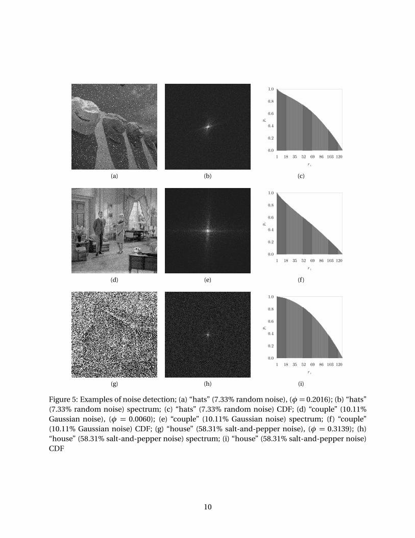
accuracy rate of 92.08%.Examples of the noisy images used in this survey are found in Figure 5. The random and

salt-and-pepper noise of Figures 5a and 5g, respectively, give rise to pronounced “humps” atthe centers of both CDFs, presented in Figures 5c and 5i, respectively. Hence, in both instances,φ correctly surpasses the noise threshold Tη. The somewhat inconsequential Gaussian noise ofFigure 5d manages to escape detection. When the intensity of this type of noise is particularlylow, the accompanying CDF tends to be rather similar to that of an untainted image, as one candeduce from Figure 5f.

Finally, the 240 blurred images were analyzed. Just as in Section 2.2, a blurred image is one inwhichφ < Tβ =−0.35. All but one of the 80 images smeared by an averaging filter were properlymarked as being blurred. This is therefore an accuracy rate of 98.75%. Perfect classification wasobserved over all 80 Gaussian-blurred images. Lastly, 66 of the 80 pictures distorted by a motionblur were found to be blurred, producing an accuracy rate of 82.50%. A motion blur tends topreserve more detail than the other two types, making it somewhat more difficult to detect. Intotal, nevertheless, 225 of the 240 blurred images were correctly found to be blurred, giving anoverall accuracy rate of 93.75% for this error.

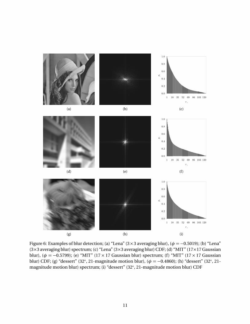
Three of the blurred images that were tested are seen in the example of Figure 6. Even aminor blur, such as the 3× 3 averaging blur of Figure 6a, is caught by the new technique. Inthis example, φ registers a value of −0.5019, below the threshold of Tβ =−0.35. Not surprising,there is also a prominent “dip” in the accompanying CDF of Figure 6c. An even more noticeable“dip” is observed in Figure 6f. This is obviously attributed to the much more destructive 17×17Gaussian blur of Figure 6d. This distortion ultimately pulls down the value of the new metric,which, in this case, measures in at φ = −0.5799. This value is also below Tβ . Lastly, in Figure6g, a motion blur is applied. This again drives down the value of φ, dropping to a value of−0.4860. Once more, this value is below the blurring threshold. As an added remark, note thedifference between the spectrum of the image corrupted by the motion blur, given in Figure 6h,and those of the other two types of blurs, given in Figures 6b and 6e. The motion blur, by itsvery nature, introduces linear-like features that run perpendicular to the direction of the blur.This contrasts with the more arbitrary distribution of points across the spectra of the other twoblurred images. In the future, it is hoped that this difference will enable an enhanced φ metricto automatically discriminate between a motion blur and an averaging or Gaussian blur. Thissort of refined classification would likely prove to be quite challenging when it comes to thethree types of noise.

Combining the results of the no-reference case, 522 of the 560 images considered, or 93.21%of them, were properly labeled. These findings underscore the strength of the new metric.

3.2 Noise and Blur Quantification

Having established the ability of the new metric to spot an error, this research next demon-strates its capacity to measure the perceived intensity of an error. This was done using thehuman user study first presented in [7, 8]. In this study, randomly chosen participants wereasked to assess the perceived quality of a series of corrupted images. Fourteen “classic” im-ages, some of which have already been encountered in this paper, were selected for this study.All of these may be seen in [7, 8]. Each of these 14 images was artificially corrupted by one ofnoise, blurring or compression [1]. This procedure was repeated five times, thereby producing

9

(a) (b)

0.0

0.2

0.4

0.6

0.8

1.0

1 18 35 52 69 86 103 120r i

p i

(c)

(d) (e)

0.0

0.2

0.4

0.6

0.8

1.0

1 18 35 52 69 86 103 120r ip i

(f)

(g) (h)

0.0

0.2

0.4

0.6

0.8

1.0

1 18 35 52 69 86 103 120r i

p i

(i)

Figure 5: Examples of noise detection; (a) “hats” (7.33% random noise), (φ = 0.2016); (b) “hats”(7.33% random noise) spectrum; (c) “hats” (7.33% random noise) CDF; (d) “couple” (10.11%Gaussian noise), (φ = 0.0060); (e) “couple” (10.11% Gaussian noise) spectrum; (f) “couple”(10.11% Gaussian noise) CDF; (g) “house” (58.31% salt-and-pepper noise), (φ = 0.3139); (h)“house” (58.31% salt-and-pepper noise) spectrum; (i) “house” (58.31% salt-and-pepper noise)CDF

10

(a) (b)

0.0

0.2

0.4

0.6

0.8

1.0

1 18 35 52 69 86 103 120r i

p i

(c)

(d) (e)

0.0

0.2

0.4

0.6

0.8

1.0

1 18 35 52 69 86 103 120r i

p i

(f)

(g) (h)

0.0

0.2

0.4

0.6

0.8

1.0

1 18 35 52 69 86 103 120r i

p i

(i)

Figure 6: Examples of blur detection; (a) “Lena” (3×3 averaging blur), (φ =−0.5019); (b) “Lena”(3×3 averaging blur) spectrum; (c) “Lena” (3×3 averaging blur) CDF; (d) “MIT” (17×17 Gaussianblur), (φ = −0.5799); (e) “MIT” (17× 17 Gaussian blur) spectrum; (f) “MIT” (17× 17 Gaussianblur) CDF; (g) “dessert” (32◦, 21-magnitude motion blur), (φ =−0.4860); (h) “dessert” (32◦, 21-magnitude motion blur) spectrum; (i) “dessert” (32◦, 21-magnitude motion blur) CDF

11

ErrorNumber of Number of Correctly Proportion of CorrectlyTest Images Classified Images Classified Images

none (error-free) 13 13 100.00%

random noise 9 8 88.89%Gaussian noise 7 4 57.14%

salt-and-pepper noise 5 5 100.0%total (noise) 21 17 80.95%

averaging blur 10 10 100.00%Gaussian blur 7 6 85.71%motion blur 4 4 100.00%total (blur) 21 20 95.24%

total 55 50 90.91%

Table 2: Experimental results for no-reference noise, blur and error-free detection usingφ (hu-man user study)

five corrupted versions of each of the 14 images. Thus, in total, 14 · 5 = 70 corrupted imageswere generated. Those tainted by compression errors are not discussed in this paper as they arenot relevant, thereby leaving only 70− 15 = 55 images to consider. Each of the human partici-pants in this experiment was shown one of the five damaged images, arbitrarily selected, fromeach of the 14 “sets” of corrupted images. They were asked to identify the quality of each imageas being either “unusable”, “poor”, “fair”, “good” or “excellent”, using the numerical values 0, 1,2, 3 and 4, respectively. These numerical scores were subsequently averaged over all 73 par-ticipants, resulting in individual mean opinion scores [30] (MOS) for each of the 55 corruptedimages. Lastly, by way of the Pearson product-moment correlation coefficient [31], the meanopinion scores were compared with the individual φ scores assigned to each of these 55 testimages. In the case of those impaired by noise, the level of correlation comes in at ρ =−0.6856,with an associated student t [24] statistic of t ∗ = −4.1048. As for the blurred images, the cor-relation stands at ρ = 0.6456, with t ∗ = 3.6850. These results attest to the genuine difficultiesencountered when attempting to perceptually quantify errors. In this research, however, this isof much lesser concern given that the focus is that of the detection, rather than the perceptualquantification, of errors. And, as the evidence of Table 2 shows, this research is again successfulwhen it comes to the issue of detecting errors. Overall, a 90.91% accuracy in classification isachieved, a value that follows just behind the strong result obtained earlier in Section 3.1.

4 Conclusion

When organized into a cumulative distribution function, frequency information allows for easyand reliable classification of images. In particular, those that are noisy, blurred or otherwiseuncorrupted may be individually separated from one another using a new metric. The exactdegree of noise or blur depends on the content of the specific image in question. Future direc-tions include refining the thresholds employed in this work, as well as distinguishing betweenthe individual types of blurring and, perhaps, noise. Color is another tempting prospect, giventhat color images offer more information than do grayscale images. This could ultimately lead

12

to even better performance when it comes to error detection. Lastly, and perhaps most signif-icant of all, is the task of verifying the implied conjecture that an uncorrupted image generallyproduces a more or less balanced CDF. At the moment, this issue has only been addressed froman empirical perspective. A more formal examination of this idea is needed.

5 Acknowledgements

This research was funded by a grant from the Natural Sciences and Engineering Research Coun-cil of Canada (NSERC). Further thanks are extended to the University of Regina Research EthicsBoard (REB) for their efforts in approving the human user study described in this work.

References

[1] Rafael Gonzalez and Richard Woods. Digital Image Processing. Prentice Hall, 2002.

[2] Milan Sonka, Vaclav Hlavac, and Roger Boyle. Image Processing, Analysis and MachineVision. Brooks/Cole, 1999.

[3] Stuart Perry, Hau San Wong, and Ling Guan. Adaptive Image Processing: A ComputationalIntelligence Perspective. CRC Press, 2002.

[4] Lynn Loomis. Calculus. Addison-Wesley, 1974.

[5] Ruud Janssen. Computational Image Quality. SPIE Press, 2001.

[6] Sabine Süsstrunk and Stefan Winkler. Color image quality on the internet. Proc. IS&T/SPIEElectronic Imaging 2004 Conf: Internet Imaging V, 5304:118–131, December 2003.

[7] Richard Dosselmann and Xue Dong Yang. No-reference image quality assessment usinglevel-of-detail. Technical Report CS 2011-2, University of Regina, Regina, Saskatchewan,Canada, May 2011.

[8] Richard Dosselmann. Image Quality Assessment using Level-of-Detail. PhD thesis, Univer-sity of Regina, 2012.

[9] Shahriar Kaisar, Sakib Rijwan, Jubayer Al Mahmud, and Muhammad Rahman. Salt andpepper noise detection and removal by tolerance based selective arithmetic mean filter-ing technique for image restoration. Int. Journal Computer Science and Network Security,8(6):271–278, June 2008.

[10] Jafar Mohammed. An improved median filter based on efficient noise detection for highquality image restoration. Second Asia Int. Conf. Modeling & Simulation, pages 327–331,May 2008.

[11] Takanori Sato, Noritaka Yamashita, Yoshinori Ito, Jianming Lu, Hiroo Sekiya, and TakashiYahagi. Impulse noise detector using absolute deviation and spatial relations between thecolor components for color images. 2006 RISP Int. Workshop Nonlinear Circuit and SignalProcessing, pages 279–282, March 2006.

13

[12] Marc Hensel, Gordon Wiesner, Bernd Kuhrmann, Thomas Pralow, and Rolf-Rainer Grigat.Motion and noise detection for adaptive spatio-temporal filtering of medical X-ray imagesequences. 14th Int. Conf. Medical Physics, 50:219–222, 2005.

[13] Bogdan Smolka. Adaptive impulsive noise removal in color images. Proc. Asia-PacificSignal and Information Processing Association Annual Summit and Conf., pages 755–764,October 2009.

[14] Jaakko Astola, Petri Haavisto, and Yrjö Neuvo. Vector median filters. Proc. IEEE, 78(4), April1990.

[15] George Luger. Artificial Intelligence: Structures and Strategies for Complex Problem Solving.Pearson, 6th edition, 2009.

[16] V. Saradhadevi and V. Sundaram. A novel two-stage impulse noise removal techniquebased on neural networks and fuzzy decision. Int. Journal Computer Applications, pages31–42, 2011.

[17] Richard Duda, Peter Hart, and David Stork. Pattern Classification. John Wiley & Sons, 2001.

[18] Zhou Wang and David Zhang. Impulse noise detection and removal using fuzzy tech-niques. IEE Electronics Letters, 33(5):378–379, February 1997.

[19] Li-Xin Wang. A Course in Fuzzy Systems and Control. Prentice Hall PTR, 1997.

[20] Pina Marziliano, Frederic Dufaux, Stefan Winkler, and Touradj Ebrahimi. Perceptual blurand ringing metrics: Application to JPEG2000. Signal Processing: Image Communication,19(2):163–172, 2004.

[21] Yun-Chung Chung, Jung-Ming Wang, Robert Bailey, Sei-Wang Chen, and Shyang-LihChang. A non-parametric blur measure based on edge analysis for image processing ap-plications. Proc. IEEE Conf. Cybernetics and Intelligent Systems, 1:356–360, 2004.

[22] Gang Cao, Yao Zhao, and Rongrong Ni. Edge-based blur metric for tamper detection. Jour-nal Information Hiding and Multimedia Signal Processing, 1(1):20–27, January 2010.

[23] Anat Levin. Blind motion deblurring using image statistics. Advances in Neural Informa-tion Processing Systems, December 2006.

[24] Donald Sanders and Robert Smidt. Statistics: A First Course. McGraw-Hill, 2000.

[25] D. Tolhurst, Y. Tadmore, and Tang Chao. Amplitude spectra of natural images. Ophthalmicand Physiological Optics, 12(2):229–232, April 1992.

[26] Renting Liu, Zhaorong Li, and Jiaya Jia. Image partial blur detection and classification.IEEE Conf. Computer Vision and Pattern Recognition, pages 1–8, 2008.

[27] Ming-Jun Chen and Alan Bovik. No-reference image blur assessment using multiscale gra-dient. Int. Workshop Quality of Multimedia Experience, pages 70–74, 2009.

14

[28] Abe Shigeo. Support Vector Machines for Pattern Classification. Springer, 2005.

[29] William Hays and Robert Winkler. Statistics: Probability, Inference, and Decision. Holt,Rinehart and Winston, 1971.

[30] Stefan Winkler. Digital Video Quality: Vision Models and Metrics. John Wiley & Sons, 2005.

[31] John Neter, Michael Kutner, Christopher Nachtsheim, and William Wasserman. AppliedLinear Statistical Models. Irwin, 1996.

15