Rich Field Photometry – Techniques and Science aka

A Deep Synoptic Study of the Stellar Populations in the Galactic Bulge: Solving the Technical Challenges

{A work in progress….}

A. Saha (NOAO) E. Olszewski, Jenna Claver, Knut Olsen, Bob Blum, Katie Kaleida, Kathy Vivas, Frank Valdes, Alistair Walker, Tom Matheson, Gautham Narayan, Todd Boroson, Steve Ridgway, Tim Axelrod, Andrea Kunder, Brenda Frye, Josh Bloom, Adam Miller, Brad Cenko, Mario Juric, David Nidever

Why study the Bulge? - Ia. • Bulges are either classical, or ‘pseudo-bulges’,

i.e. boxy/peanut-shaped (X in projection) or a combination of both

– Theories depends on dynamical history, e.g. mergers

• The Galaxy now known to be the latter kind, including a bar (as ~ 50% of spirals)

– Formed from buckling of inner disk?

Why study the Bulge? - Ib.

“Models are now able to produce realistic analogs of the Milky Way bulge, and have reached the point at which the spatial distribution of component populations is the key diagnostic between scenarios”

--- Will Clarkson

Calls for disambiguation of “classical” and “pseudo-bulge” components using stellar populations, specifically as manifest in CMDs.

Why study the Bulge? - II.

• A rich zoo of stars and stellar populations in a relatively compact field.

• Going deep can provide an interesting discovery space, especially in the time domain

• A great training ground for LSST relevant issues: – Crowded field photometry

– Response to variable phenomena

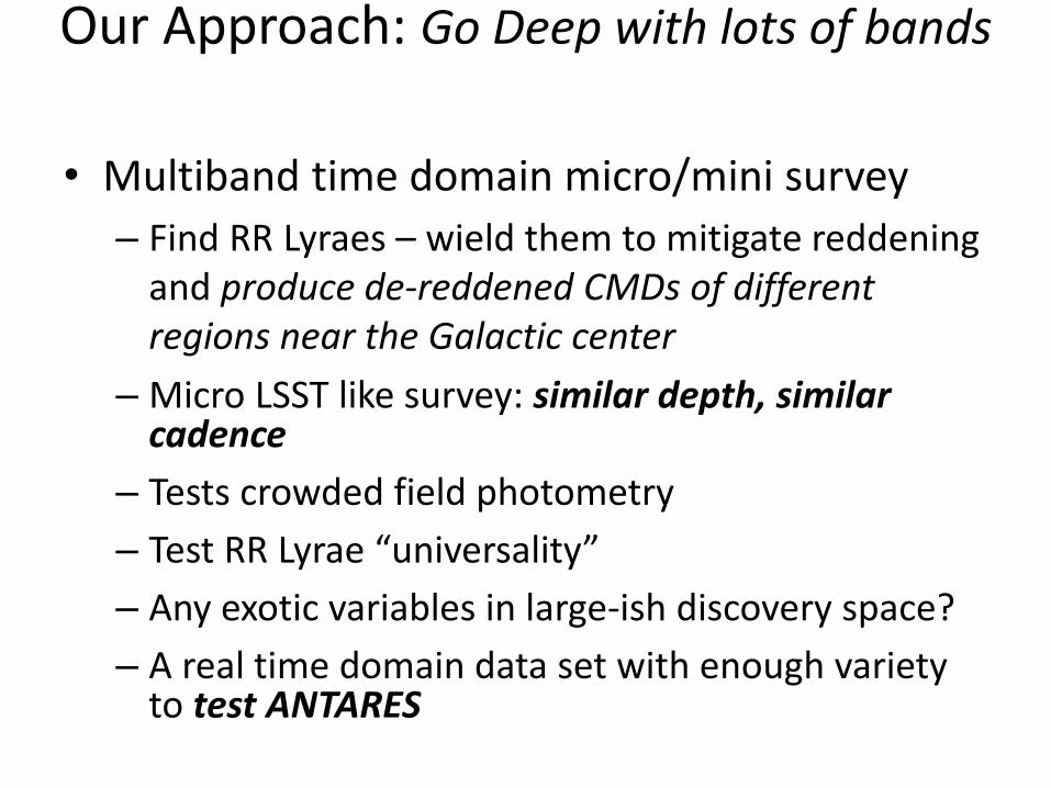
Our Approach: Go Deep with lots of bands

• Multiband time domain micro/mini survey

– Find RR Lyraes – wield them to mitigate reddening and produce de-reddened CMDs of different regions near the Galactic center

– Micro LSST like survey: similar depth, similar cadence

– Tests crowded field photometry

– Test RR Lyrae “universality”

– Any exotic variables in large-ish discovery space?

– A real time domain data set with enough variety to test ANTARES

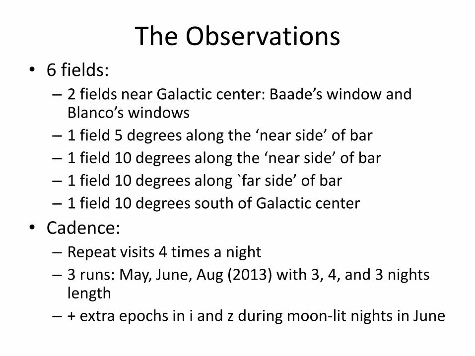
The Observations • 6 fields:

– 2 fields near Galactic center: Baade’s window and Blanco’s windows

– 1 field 5 degrees along the ‘near side’ of bar

– 1 field 10 degrees along the ‘near side’ of bar

– 1 field 10 degrees along `far side’ of bar

– 1 field 10 degrees south of Galactic center

• Cadence: – Repeat visits 4 times a night

– 3 runs: May, June, Aug (2013) with 3, 4, and 3 nights length

– + extra epochs in i and z during moon-lit nights in June

DECam passbands

Wavelength ˚

Rela

tive

Fla

m

Dim

en

sion

less

Th

rou

gh

pu

t

g band image, 100s Baade’s window

U band image 300s Baade’s window Note intricate structure in Reddening with scales less Than 1 arc-minute!

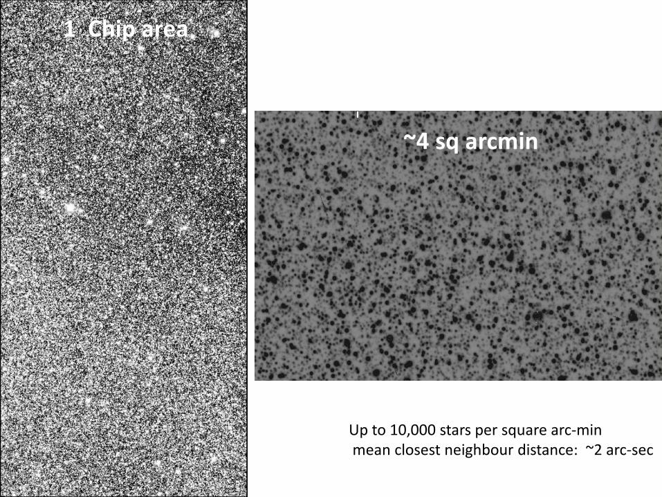
~4 sq arcmin

1 Chip area

Up to 10,000 stars per square arc-min mean closest neighbour distance: ~2 arc-sec

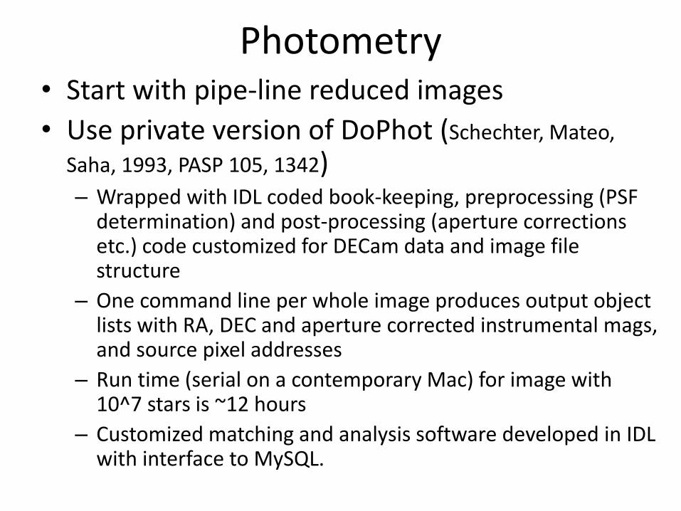
Photometry • Start with pipe-line reduced images

• Use private version of DoPhot (Schechter, Mateo,

Saha, 1993, PASP 105, 1342) – Wrapped with IDL coded book-keeping, preprocessing (PSF

determination) and post-processing (aperture corrections etc.) code customized for DECam data and image file structure

– One command line per whole image produces output object lists with RA, DEC and aperture corrected instrumental mags, and source pixel addresses

– Run time (serial on a contemporary Mac) for image with 10^7 stars is ~12 hours

– Customized matching and analysis software developed in IDL with interface to MySQL.

Raw comparison of photomtry from 2 r images. 6.4 million matched objects. Many specious cases.

Same comparison, but using a priori criteria on DoPhot output to clean pathologies.

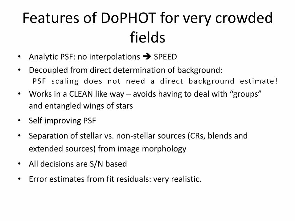
Features of DoPHOT for very crowded fields

• Analytic PSF: no interpolations SPEED

• Decoupled from direct determination of background: PSF scal ing does not need a direct background estimate!

• Works in a CLEAN like way – avoids having to deal with “groups”

and entangled wings of stars

• Self improving PSF

• Separation of stellar vs. non-stellar sources (CRs, blends and

extended sources) from image morphology

• All decisions are S/N based

• Error estimates from fit residuals: very realistic.

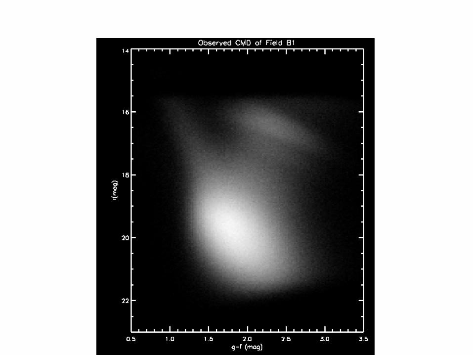
CMDs from OGLE experiment

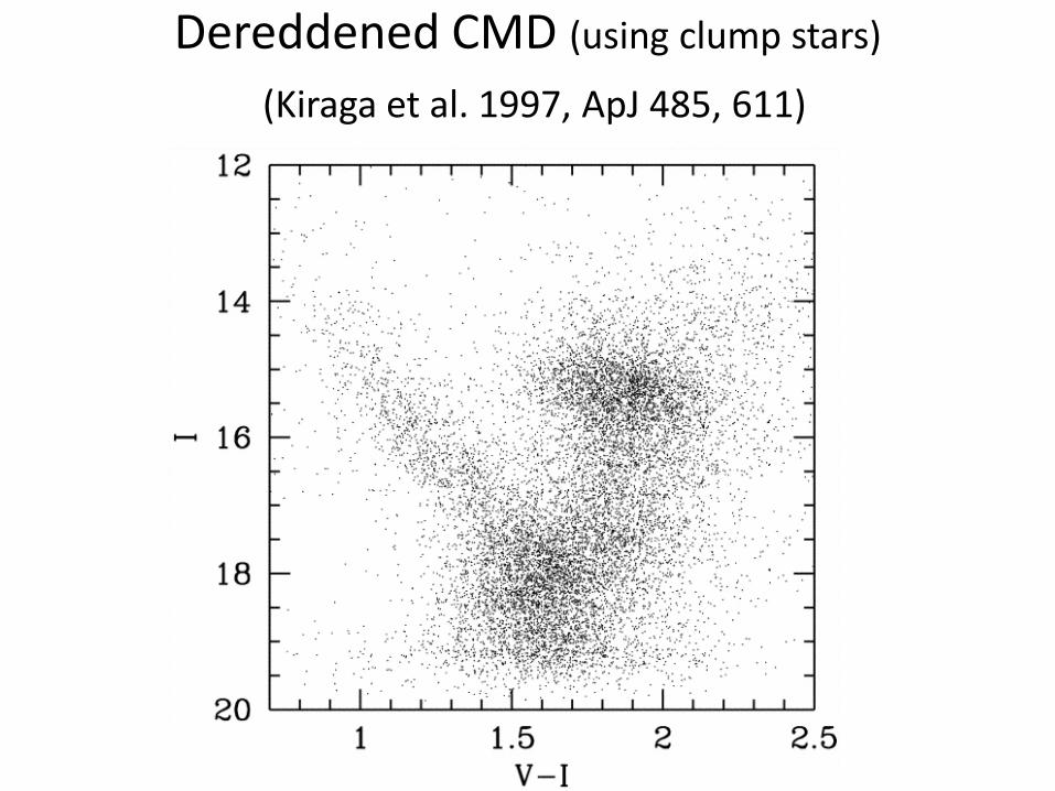
Dereddened CMD (using clump stars)

(Kiraga et al. 1997, ApJ 485, 611)

Organize into Data Base

• Choose output from deepest r images obtained in photometric conditions and co-average photometry into a master template

• Match objects from each epoch to master template

• Store matched photometry, epoch by epoch, and for each passband in a MySQL database

• Apply calibration to photometry, and process to find variables.

Finding Variable Candidates

• For each object in each band look at photometry variance across epochs (~30 epochs per band) – Use a bootstrap chi-square to flag variables using DoPHOT

reported errors

– Resulted in ~7500 candidate variables !!! • > 90% can be visually confirmed (from looking at a few hundred)

• Visually blink brightest and faintest apparitions (IDL) – bookkeeping in database allows quick lookup

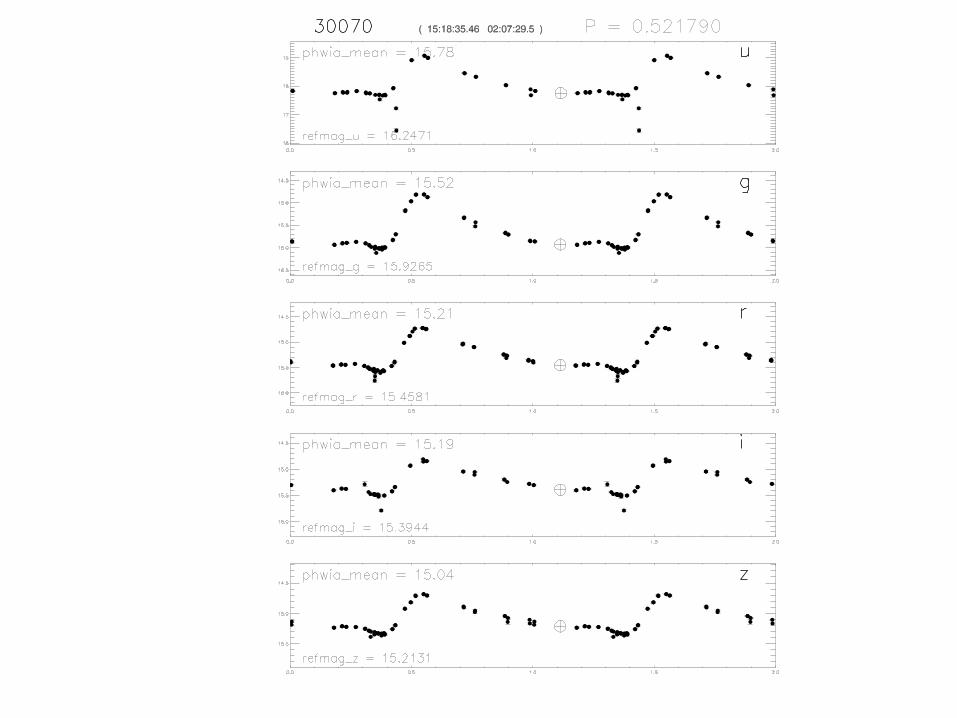
• If confirmed, perform period analysis – IDL coded visual interactive method combining FFT and

Lafler-Kinman algorithms

– Works simultaneously on data from ALL available bands, producing a JOINT periodogram

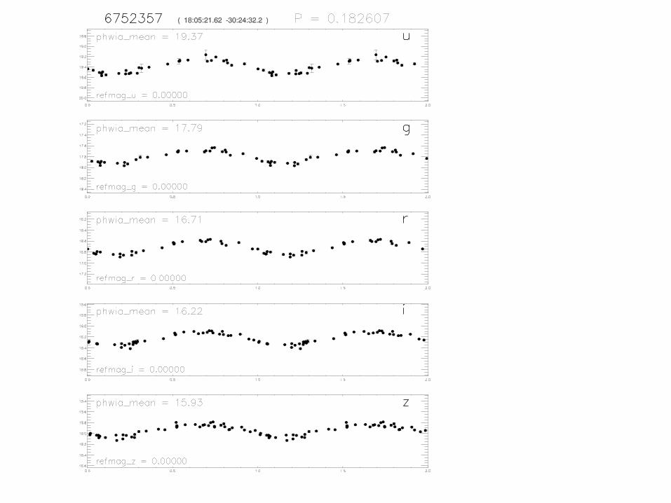
Also shows minimum light photometry

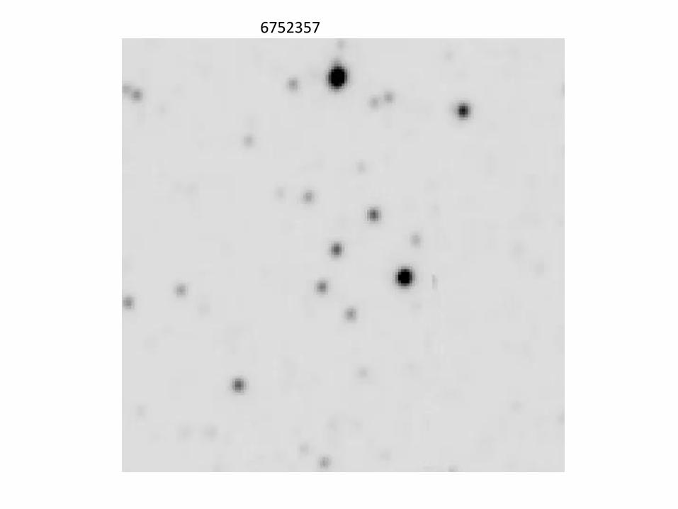
6752357

Lafler-Kinman

Periodograms of the Same Object with Different Algorithms (the problem of sparse data)

Fourier Transform

Combined Algorithm and Light Curves

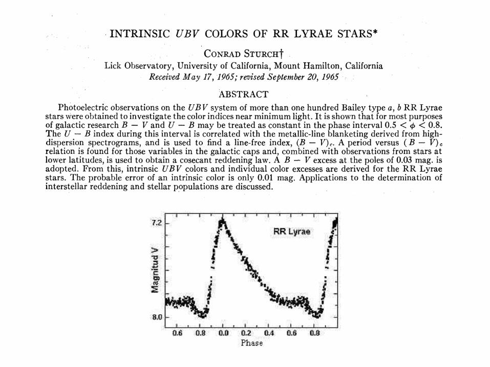
Sturch’s Findings (slightly restated)

1. The colors [ (U-B), (B-V) ] of fundamental mode RR Lyraes do not change in the phase range 0.5 to 0.8 (minimum light) by more than ~0.02 mag.

- Star to star variations correlate with metallicity (line-blanketing) and weakly with Period

2. In high Galactic latitude (b > 50o) fields, fundamental mode RR Lyrae star colors at minimum light show very small scatter, which correlates with metallicity.

3. The TEMPERATURES at minimum light of FM RR Lyrae stars is constant to better than 100o K. Reconfirmed in other work by Oke, and later (unpublished) by Saha

4. Therefore intrinsic colors of FM RR Lyraes at minimum light are predictable to a few times 0.01 mag

RR Lyraes, via Sturch’s findings, were used in the calibration of the HI vs reddening by Burstein & Heiles 1978, ApJ 225, 40.

Sturch’s rule E(B-V) = (B-V)=(0.5 to 0.8) + 0.0122 S

- 0.00045(S)2 - 0.185P - 0.356

(gives results good to ~0.01 mag in E(B-V) !!

BUT ---You (may) have to know metallicity!

SDSS colors g-r, r-i, r-z, and i-z are progressively freer of line blanketing.

In any case we have to recalibrate in the SDSS (or native DECam system)

Fiducial Minimum Light Colors in ugriz

• Use observations of globular cluster M5

• Apply identical process to find RR Lyrae stars and measure colors at minimum light

– With fewer available epochs, cross matching with known objects and ephemerides helps

– 45 fundamental mode RR Lyrae with light curves recovered, of which 3 are much fainter and not M5 members.

DA-WDs as standards

• HST has been using them since 1996, even before the compelling evidence was gathered!

• SED obtainable from spectra (via Balmer line fitting, Holberg & Bergeron) and NLTE modeling

– Expected accuracy few milli-mag

• DA-WDs in use are bright, and close by – reddening ignorable at few milli-mag level.

– Too bright for dynamic range of modern large telescopes

– Zero-points need to be determined above atmosphere

Generate Model SED Derive Synthetic Colors

3000

4000

5000

6000

7000

8000

log

F GMOS Spectrum

Model SED

1300

0

1400

0

1500

0

1600

0

1700

0

F625W

%T

hro

ugh

pu

t

F160WF775WF336W F475W

WFC3/UVIS2WFC3/UVIS2 WFC3/IRWFC3/IR

Wavelength (A)

Rms residual = .004 mag Extrema: +/- .007 mag .

First Results

Two free parameters to reconcile predicted SED and measured HST mags: a) A common zero-point b) A reddening parameter, ( e.g. AV)

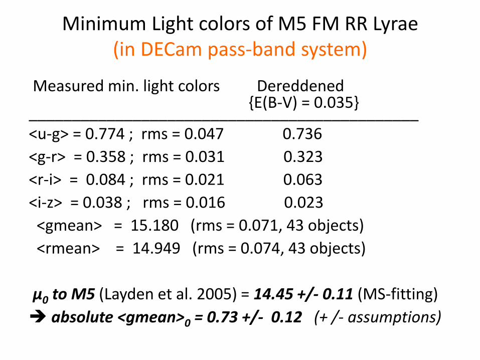
Minimum Light colors of M5 FM RR Lyrae (in DECam pass-band system)

Measured min. light colors Dereddened {E(B-V) = 0.035} _____________________________________________ <u-g> = 0.774 ; rms = 0.047 0.736

<g-r> = 0.358 ; rms = 0.031 0.323

<r-i> = 0.084 ; rms = 0.021 0.063

<i-z> = 0.038 ; rms = 0.016 0.023

<gmean> = 15.180 (rms = 0.071, 43 objects)

<rmean> = 14.949 (rms = 0.074, 43 objects)

μ0 to M5 (Layden et al. 2005) = 14.45 +/- 0.11 (MS-fitting)

absolute <gmean>0 = 0.73 +/- 0.12 (+ /- assumptions)

Empirical Period dependance of minimum (r-z) for M5

Slope = 0.17 Rms ~ 0.02 mag

Caveats/Considerations

• DECam passbands not identical to SDSS

– Observations calibrated to a native system using DA white dwarfs

– Which is why we observed M5, rather than use SDSS colors of RR Lyrae

• Need to examine minimum light color variation with metallicity

Wavelength ˚

Rela

tive

Fla

m

Dim

en

sion

less

Th

rou

gh

pu

t

Teff = 6250K, log_g=2.0 Filter Z0_Zm1 Z0_Zm2 Z0_Zp0.5 u 0.248 0.331 -0.230 g -0.020 -0.040 -0.001 r -0.071 -0.108 0.049 i -0.057 -0.088 0.042 z -0.052 -0.079 0.036 y -0.055 -0.083 0.040

r-z is insensitive to metallicity

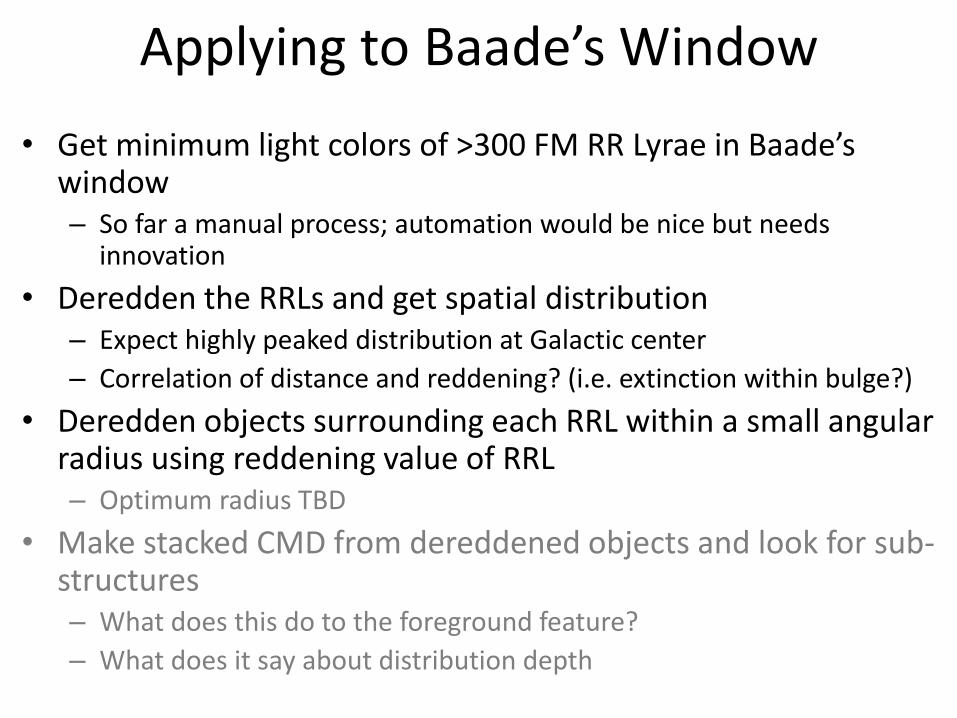
Applying to Baade’s Window

• Get minimum light colors of >300 FM RR Lyrae in Baade’s window – So far a manual process; automation would be nice but needs

innovation

• Deredden the RRLs and get spatial distribution – Expect highly peaked distribution at Galactic center

– Correlation of distance and reddening? (i.e. extinction within bulge?)

• Deredden objects surrounding each RRL within a small angular radius using reddening value of RRL – Optimum radius TBD

• Make stacked CMD from dereddened objects and look for sub-structures – What does this do to the foreground feature?

– What does it say about distribution depth

Observed Color excess slopes agree with Yuan et al. reddening law (Yuan et al. 2013, MNRAS 430, 2188)

But what about non-zero intercepts? Significant? Effect of metallicities?

Metallicity Effects

• Walker & Terndrup 1991, ApJ 378, 119

M5 metallicity –

values in literature range between:

[Fe/H] = -1.1 to -1.3

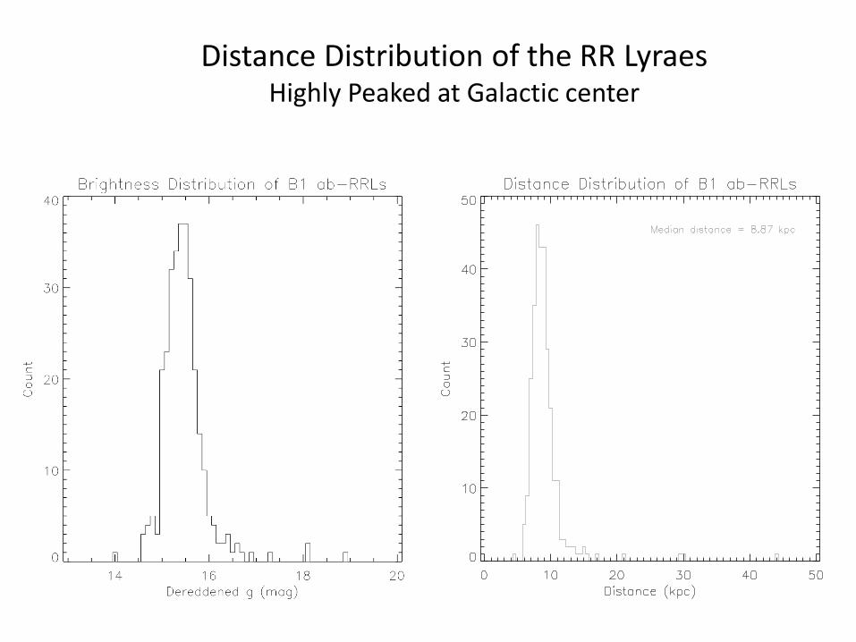
Distance Distribution of the RR Lyraes Highly Peaked at Galactic center

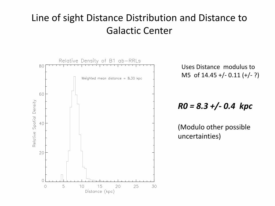
Line of sight Distance Distribution and Distance to Galactic Center

Uses Distance modulus to M5 of 14.45 +/- 0.11 (+/- ?)

R0 = 8.3 +/- 0.4 kpc (Modulo other possible uncertainties)

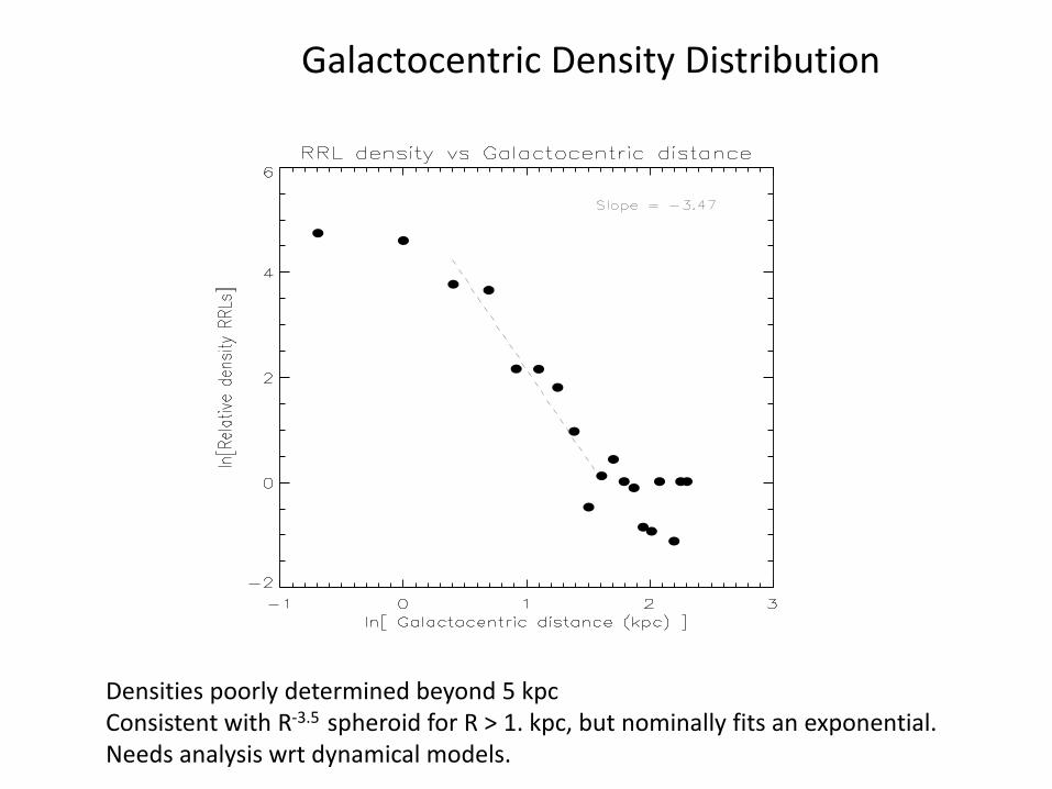
Galactocentric Density Distribution

Densities poorly determined beyond 5 kpc Consistent with R-3.5 spheroid for R > 1. kpc, but nominally fits an exponential. Needs analysis wrt dynamical models.

Line of Sight Reddening Contribution

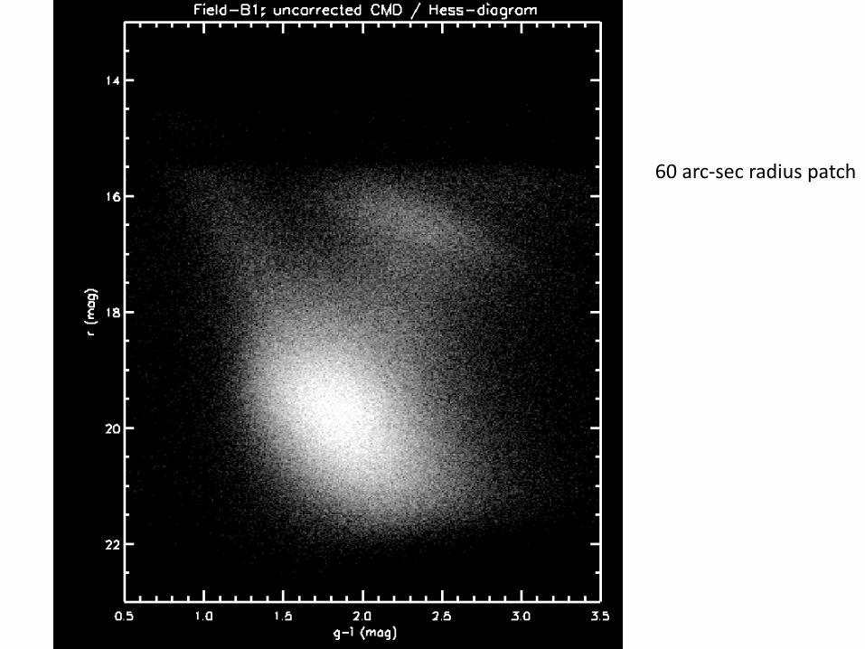
60 arc-sec radius patch

60 arcsec radius patch

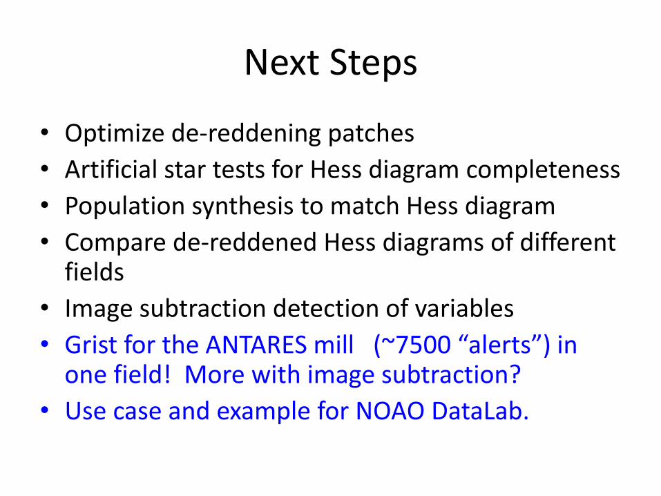
Next Steps

• Optimize de-reddening patches

• Artificial star tests for Hess diagram completeness

• Population synthesis to match Hess diagram

• Compare de-reddened Hess diagrams of different fields

• Image subtraction detection of variables

• Grist for the ANTARES mill (~7500 “alerts”) in one field! More with image subtraction?

• Use case and example for NOAO DataLab.

The Galactic Bulge

• Traditional views and current paradigms

• a figure + top down view of los and bar

• Is bar formed from buckling of the disk?

• What a CMD can reveal

• Problems with study : sky coverage & reddening

• Past work, especially OGLE& Macho using clump stars

Interstellar Extinction

Rich Field Photometry – Techniques and Science aka

A Deep Synoptic Study of the Stellar Populations in the Galactic Bulge:

Solving the Technical Challenges

{A work in progress….}

A.Saha

E. Olszewski, Jenna Claver, Knut Olsen, Bob Blum, Katie Kaleida, Kathy Vivas, Frank Valdes, Alistair Walker, Tom Matheson, Gautham

Narayan, Todd Boroson, Steve Ridgway, Tim Axelrod, Andrea Kunder, Brenda Frye, Josh Bloom, Adam Miller, Brad Cenko, Mario

Juric, David Nidever