Ricci flow and nonnegativity of sectional curvature

Mathematical Research Letters 11, 883–904 (2004)

RICCI FLOW AND NONNEGATIVITY

OF SECTIONAL CURVATURE

Lei Ni

Abstract. In this paper, we extend the general maximum principle in [NT3]to the time dependent Lichnerowicz heat equation on symmetric tensors coupledwith the Ricci flow on complete Riemannian manifolds. As an application weexhibit complete Riemannian manifolds with bounded nonnegative sectional cur-vature of dimension greater than three such that the Ricci flow does not preservethe nonnegativity of the sectional curvature, even though the nonnegativity of thesectional curvature was proved to be preserved by Hamilton in dimension three.This fact is proved through a general splitting theorem on the complete family ofmetrics with nonnegative sectional curvature, deformed by the Ricci flow.

Introduction

The Ricci flow has been proved to be an effective tool in the study of thegeometry and topology of manifolds. One of the good properties of the Ricciflow is that it preserves the ‘nonnegativity’ of various curvatures. In dimensionthree, Hamilton [H1] proves that on compact manifolds the Ricci flow preservesthe nonnegativity of the Ricci curvature and the sectional curvature. Usingthis property and the quantified version, curvature pinching estimate, it wasproved in [H1] that the normalized Ricci flow converges to a Einstein metric ifthe initial metric has positive Ricci curvature. In particular, it implies that asimply-connected compact three-manifold is diffeomorphic to the three sphereif it admits a metric with positive Ricci curvature. One can refer [Ch] for anupdated survey and [P2] for some recent developement on the Ricci flow onthree manifolds. Later in [H2] it was proved that the Ricci flow also preservesthe nonnegativity of the curvature operator in all dimensions (on compact man-ifolds). In the Kahler case, Bando and Mok [B, M] proved that the flow alsopreserves the nonnegativity of the holomorphic bisectional curvature. The Ricciflow on complete manifolds was initiated in [Sh2]. In [Sh3] Shi generalized theabove mentioned result of Bando and Mok to the complete Kahler manifoldswith bounded curvature. Interesting applications were also obtained therein.

In this paper, we shall study the topological consequences of the assumptionthat Ricci flow preserves the nonnegativity of the sectional curvature on completeRiemannian manifolds. The basic method is to study the heat equation, time

Received May 3, 2003. Revised August 2004.Research partially supported by NSF grant DMS-0328624, USA.

883

884 LEI NI

dependent, deformation of the Busemann function via the new tensor maximumprinciple proved in [NT3]. The maximum principle of this type was first provedby Hamilton for compact manifolds [H2]. The proof of [H2] can be generalizedto the complete noncompact manifolds with bounded curvature with additionalassumption that the tensor satisfying certain heat equation is uniformly boundedon the space-time. See for example [H3, Theorem 5.3], [NT2, Proposition 1.1]and [Ca]. However in the study of the deformation of a continuous function,the Busemann function (with respect to all rays from a fixed point) in our case,one in general can not expect uniform pointwise control of its Hessian since theBusemann function is not even differentiable in general. Therefore one needsa more general maximum principle than those developed by Hamilton in [H3].This is the main technical difficulty. This difficulty was resolved in [NT3] andan (optimal in a certain sense) maximum principle was established there forthe time-independent heat equation. The tensor maximum principle proved inTheorem 2.1 of this paper is a time-dependent analogue of the correspondingresult, Theorem 2.1 in [NT3].

By studying the deformation of the Busemann function, we shall prove thaton a simply-connected complete Riemannian manifolds with bounded nonneg-ative sectional curvature, if the Ricci flow preserves the nonnegativity of thesectional curvature, then the manifold splits as the product of a compact man-ifold with nonnegative sectional curvature with a complete manifold which isdiffeomorphic to the Euclidean space. As a consequence of such splitting result,we give examples of complete Riemannian manifolds with bounded nonnegativesectional curvature of dimension ≥ 4 such that the Ricci flow does not preservethe nonnegativity of the sectional curvature. As far as we know, this is the firstexample of this kind even though this is believed to be the case by the experts.Noticing that in dimension three the Ricci flow does preserve the nonnegativityof the sectional curvature by [H1] on compact manifolds and complete manifoldswith bounded curvature. Another application of our approach is a classificationof complete manifolds with bounded nonnegative curvature operator, a resultwhich has been previously established in [N] using different methods withoutassuming the boundedness of the curvature (see also [ CC, CY, GaM, H2], butmore importantly [MM, SiY] for the compact case). The use of the heat equationdeformation of Busemann functions to study the structure of complete manifoldswas initiated in [NT3]. Therefore this paper can be viewed as a continuationof the pervious work. The difference between current paper and [NT3] is thatwe have to consider the heat equation with respect to metrics evolved by theRicci flow in order to show that the Hessian of the solution to the heat equationsatisfies the Lichnerowicz heat equation. Therefore we have to derive the heatkernel estimate of Li-Yau type (cf. [LY]) for the time dependent heat equation.The estimate of this type was considered before in [Gr1, Sa] for a fixed com-plete Riemannian metric satisfying the volume doubling properties for the ballsand the Neumann-Poincare inequality. However, the heat equation consideredhere does not belong to the classes considered in the previous cases (see Remark

RICCI FLOW AND NONNEGATIVE CURVATURE 885

1.1 for more details). Therefore we devote the first section in establishing theheat kernel estimate as well as the Harnack inequality for the time dependentheat equation, following the approach of Grigoy’an in [Gr1]. The result itselfmaybe has its own interests. There exists also related (weaker) lower boundestimates on the fundamental solution of time-dependent heat equation in [Gu]by Guenther.

1. Time-dependent heat equation

Let (M, g0ij(x)) be a complete Riemannian manifold (of dimension n) with

bounded curvature tensor. We denote k0 to be the upper bound of |Rijkl|2, thecurvature tensor of g0. By [Sh2, Theorem 1.1, p. 224] we know that there existsa constant T (n, k0) > 0 such that the Ricci flow

(1.1)∂

∂tgij(x, t) = −2Rij(x, t)

has solution on M × [0, T ]. Moreover, there exists A′m = A′

m(n, m, k0) such thatfor all (x, t) ∈ M × [0, T ],

(1.2) ‖∇mRijkl‖2(x, t) ≤ A′m

tm.

In particular,

(1.3) ‖Rijkl‖(x, t) ≤√

A0.

The argument of [H2, H3] (see also [NT2, Proposition 1.1]) can be adaptedto show that gij(x, t) has nonnegative curvature operator if the initial metricgij(x, 0) has the nonnegative curvature operator. We are going to study theinitial value problem of the heat equation

(1.4)(

∂

∂t− ∆

)v(x, t) = 0

with initial value v(x, 0) = u(x). Here ∆v = gij(x, t)vij , where vij denotes theHessian of v. Namely ∆ is time-dependent. The following lemma is well-knownto experts. For example, it was known and used in [CH] by Chow and Hamil-ton in their study of the linear trace differential Harnack or Li-Yau-Hamiltoninequality for the Ricci flow.

Lemma 1.1. Let v(x, t) be a solution to (1.4). Then the complex Hessianvij(x, t) satisfies

(1.5)(

∂

∂t− ∆

)vij = 2Ripjqvpq − Ripvpj − Rpjvip.

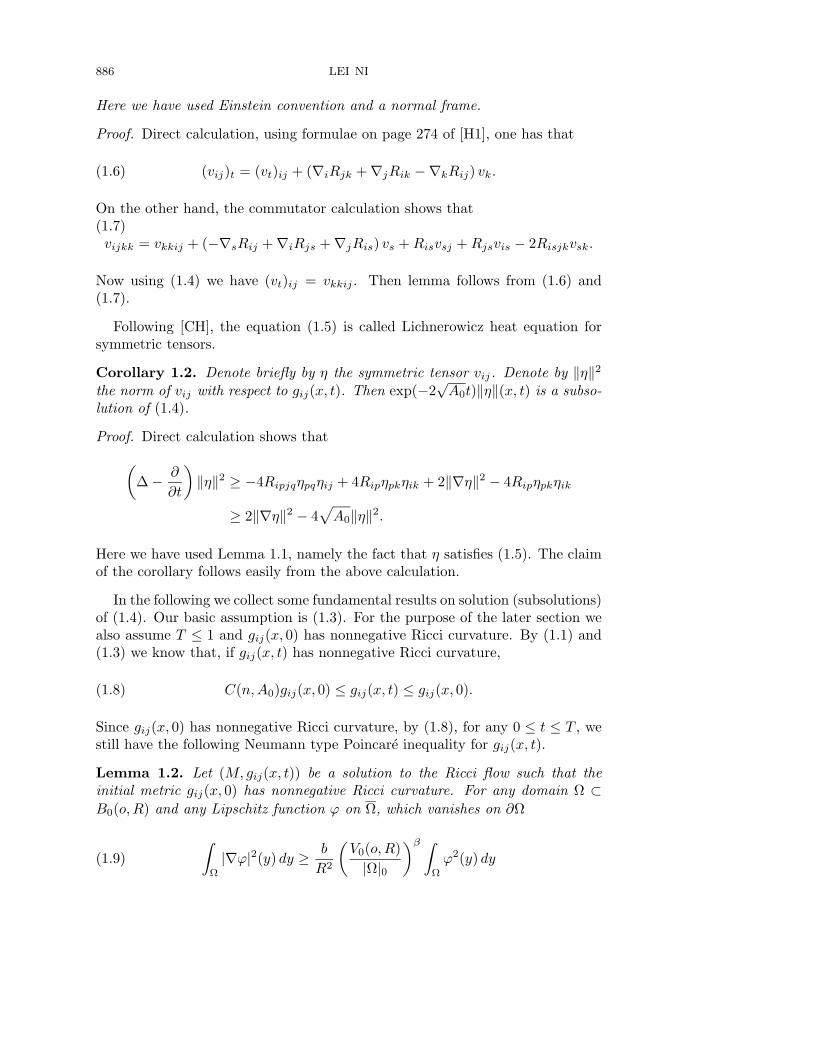
886 LEI NI

Here we have used Einstein convention and a normal frame.

Proof. Direct calculation, using formulae on page 274 of [H1], one has that

(1.6) (vij)t = (vt)ij + (∇iRjk + ∇jRik −∇kRij) vk.

On the other hand, the commutator calculation shows that(1.7)vijkk = vkkij + (−∇sRij + ∇iRjs + ∇jRis) vs + Risvsj + Rjsvis − 2Risjkvsk.

Now using (1.4) we have (vt)ij = vkkij . Then lemma follows from (1.6) and(1.7).

Following [CH], the equation (1.5) is called Lichnerowicz heat equation forsymmetric tensors.

Corollary 1.2. Denote briefly by η the symmetric tensor vij. Denote by ‖η‖2

the norm of vij with respect to gij(x, t). Then exp(−2√

A0t)‖η‖(x, t) is a subso-lution of (1.4).

Proof. Direct calculation shows that(∆ − ∂

∂t

)‖η‖2 ≥ −4Ripjqηpqηij + 4Ripηpkηik + 2‖∇η‖2 − 4Ripηpkηik

≥ 2‖∇η‖2 − 4√

A0‖η‖2.

Here we have used Lemma 1.1, namely the fact that η satisfies (1.5). The claimof the corollary follows easily from the above calculation.

In the following we collect some fundamental results on solution (subsolutions)of (1.4). Our basic assumption is (1.3). For the purpose of the later section wealso assume T ≤ 1 and gij(x, 0) has nonnegative Ricci curvature. By (1.1) and(1.3) we know that, if gij(x, t) has nonnegative Ricci curvature,

(1.8) C(n, A0)gij(x, 0) ≤ gij(x, t) ≤ gij(x, 0).

Since gij(x, 0) has nonnegative Ricci curvature, by (1.8), for any 0 ≤ t ≤ T , westill have the following Neumann type Poincare inequality for gij(x, t).

Lemma 1.2. Let (M, gij(x, t)) be a solution to the Ricci flow such that theinitial metric gij(x, 0) has nonnegative Ricci curvature. For any domain Ω ⊂B0(o, R) and any Lipschitz function ϕ on Ω, which vanishes on ∂Ω

(1.9)∫

Ω

|∇ϕ|2(y) dy ≥ b

R2

(V0(o, R)|Ω|0

)β ∫Ω

ϕ2(y) dy


for some positive constants β, b which only depends on n and A0. Here |∇ϕ|2 iscalculated using gij(x, t), while |Ω|0, the volume of Ω, and V0(o, R), the volumeof B0(o, R), are calculated using gij(x, 0).

Proof. The lemma follows easily from Theorem 1.4 of [Gr1]. The point is thatonly the weak form Neumann-Poincare inequality and the volume doubling prop-erty are needed in the proof of Theorem 1.4 of [Gr1]. Since gij(x, 0) has nonneg-ative Ricci curvature these two properties hold for (M, gij(x, 0)). On the otherhand, the metric gij(x, t) is equivalent to gij(x, 0). Therefore these two sufficientproperties preserve.

Remark 1.1. Here we assume that gij(x, 0) has nonnegative Ricci curvature tomake our presentation easier. In fact, one can replace it by assuming (M, gij(x, 0))satisfies (1.9) and a volume doubling property for balls as in [Gr1]. This appliesto some other results in this section.

The next result is a mean value inequality. The proof is just a modificationof the one in [Gr1] for the time-independent heat equation. Note that it isknown from [H1], applying the maximum principle for functions, that the scalarcurvature R(x, t) of gij(x, t) is nonnegative, under the assumption that gij(x, 0)has nonnegative Ricci/scalar curvature.

Theorem 1.1. Let (M, g(t)) be as in Lemma 1.2. Let w(x, t) be a smoothfunction satisfying

(1.10)(

∆ − ∂

∂t

)w(x, t) ≥ 0

on∐√

t with t ≤ T , where∐

R = B0(x, R)× (0, R2) and Bτ (x,√

t) is the ball ofradius

√t with respect to gij(x, τ). Then

(1.11) w2+(x, t) ≤ C(n, A0, T )

V0(x,√

t)t

∫ t

0

∫B0(x,

√t)

w2+(y, τ) dydτ

Here w+ = max0, w, V0(x, r) denotes the volume of B0(x, r) with respect togij(x, 0).

Proof. We essentially repeat the argument of the proof of Theorem 3.1 in [Gr1].The key to the argument is the fact that gij(x, t) satisfying the Neumann-Poincare inequality (1.9) and the volume double property for balls. We havethese two properties if we assume that the initial metric has nonnegative Riccicurvature. To make the iteration argument work using Lemma 1.2 we needalso to prove that the Lemma 3.1 of [Gr1] still holds for our case. In fact, forany R ≤

√t, let φ(x, t) be a cut-off function supported in B0(x, R) such that

φ(x, 0) = 0. For θ > 0, let wθ = (w − θ)+. Multiplying wθφ2 on both sides of

888 LEI NI

(1.10) we have that

∫w≥θ

wtwθφ2 dy ≤

∫w≥θ

(∆w)wθφ2 dy

= −2∫w≥θ

〈∇wθ,∇φ〉wθφ dy −∫w≥θ

|∇wθ|2φ2 dy

= −∫w≥θ

|∇(wθφ)|2 dy +∫

M

|∇φ|2w2θ dy.

(1.12)

Integrating the time variable and noticing that φ ∈ C∞0 (B0(x, R)) we have that∫ t

0

∫B0(x,R)

wθ(wθ)τφ2 dydτ ≤ −∫ t

0

∫B0(x,R)

|∇(wθφ)|2 dydτ +∫ t

0

∫B0(x,R)

|∇φ|2w2θ dydτ.

The left hand side above equals to

12

∫ t

0

∫B0(x,R)

(w2θ)τφ2 dydτ =

(12

∫B0(x,R)

w2θφ dy

)(t) −

(12

∫B0(x,R)

w2θφ dy

)(0)

+∫ t

0

∫B0(x,R)

w2θ

(−φτφ +

12R(y, τ)φ2

)dydτ.

Combining the above two inequalities and using the fact R ≥ 0 we have that(1.13)∫

B0(x,R)

w2θφ2 dy

∣∣∣∣∣t

+2∫ t

0

∫B0(x,R)

|∇(wθφ)|2dydτ ≤ 2∫ t

0

∫B0(x,R)

w2θ

(|∇φ|2 + |φφτ |

)dydτ.

Similarly, one can prove Lemma 3.2 of [Gr1], noticing that Lemma 1.2 holds formetric gij(x, t). Then the iteration scheme in [Gr1] can be applied to completethe proof of the theorem.

Next is the Harnack inequality for positive solutions. Let v be a positivesolution to (1.4) on

∐8R where

∐R = B0(x, R) × (0, R2).

Theorem 1.2. Let (M, gij(x, t)) be as in Lemma 1.2. Then there exists a con-stant γ = γ(n, A0) > 0 such that

(1.14) v(x, 64R2) ≥ γ supB0(x,R)×(3R3,4R2)

v.

Proof. The proof follows similarly as the proof of Theorem 4.1 in [Gr1]. SinceLemma 4.2–4.4 in [Gr1] are robust enough to be adapted to the current situationwe only need to establish the following result corresponding to Lemma 4.1 of[Gr1].


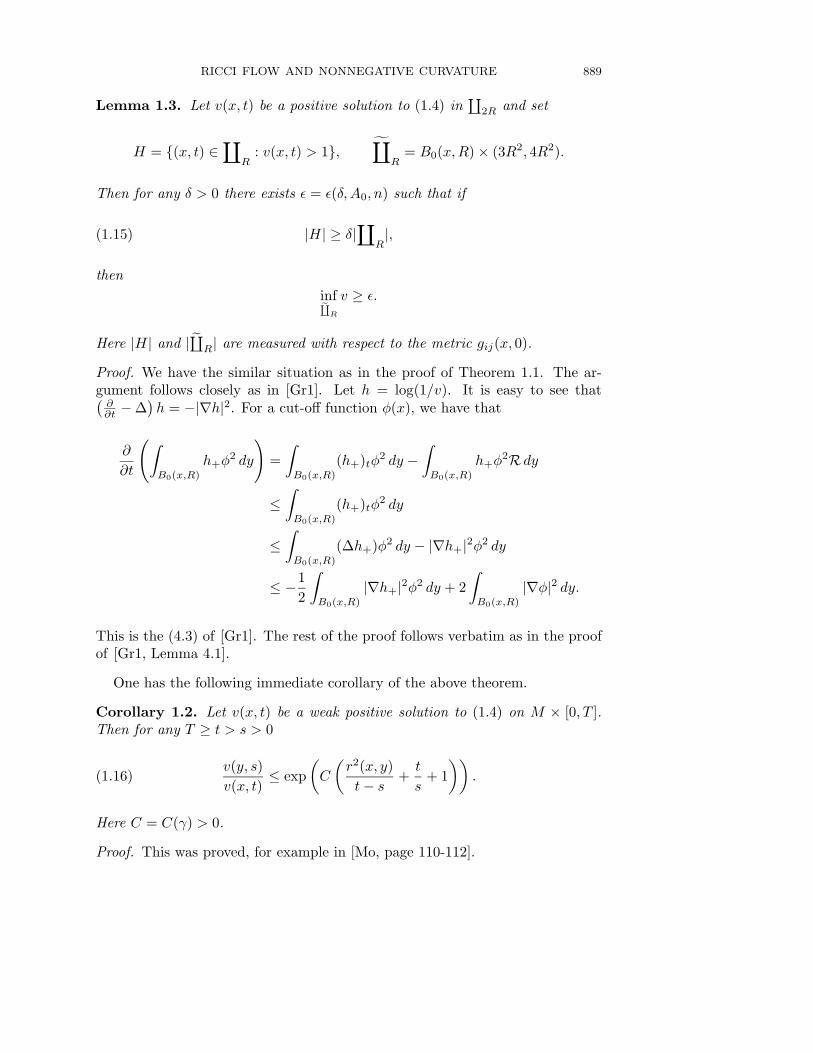
Lemma 1.3. Let v(x, t) be a positive solution to (1.4) in∐

2R and set

H = (x, t) ∈∐

R: v(x, t) > 1,

∐R

= B0(x, R) × (3R2, 4R2).

Then for any δ > 0 there exists ε = ε(δ, A0, n) such that if

(1.15) |H| ≥ δ|∐

R|,

theninf∐

R

v ≥ ε.

Here |H| and |∐

R| are measured with respect to the metric gij(x, 0).

Proof. We have the similar situation as in the proof of Theorem 1.1. The ar-gument follows closely as in [Gr1]. Let h = log(1/v). It is easy to see that(

∂∂t − ∆

)h = −|∇h|2. For a cut-off function φ(x), we have that

∂

∂t

(∫B0(x,R)

h+φ2 dy

)=

∫B0(x,R)

(h+)tφ2 dy −

∫B0(x,R)

h+φ2R dy

≤∫

B0(x,R)

(h+)tφ2 dy

≤∫

B0(x,R)

(∆h+)φ2 dy − |∇h+|2φ2 dy

≤ −12

∫B0(x,R)

|∇h+|2φ2 dy + 2∫

B0(x,R)

|∇φ|2 dy.

This is the (4.3) of [Gr1]. The rest of the proof follows verbatim as in the proofof [Gr1, Lemma 4.1].

One has the following immediate corollary of the above theorem.

Corollary 1.2. Let v(x, t) be a weak positive solution to (1.4) on M × [0, T ].Then for any T ≥ t > s > 0

(1.16)v(y, s)v(x, t)

≤ exp(

C

(r2(x, y)t − s

+t

s+ 1

)).

Here C = C(γ) > 0.

Proof. This was proved, for example in [Mo, page 110-112].

890 LEI NI

Theorem 1.3. Let (M, gij(x, t)) be a complete solution to the Ricci flow withbounded curvature. Assume that gij(x, t) has nonnegative Ricci curvature. LetH(x, y, t) be the minimal positive heat kernel of the heat equation (1.4). Thenthere exist positive constants C1, C2 and D1, D1 such that(1.17)

C11

V0(x,√

t)exp

(−D2

r2(x, y)t

)≤ H(x, y, t) ≤ C2

1V0(x,

√t)

exp(−D1

r2(x, y)t

).

Here V0(x, a) and r(x, y) denote the volume of B0(x, a) and distance betweenx and y, with respect to gij(x, 0), respectively. D1 < 1

4 is a absolute constant.D2 = D2(γ), Ci = Ci(n, D1, D2, A0).

Proof. It is easy to see that for any t > 0,∫M

H(x, y, t) dy ≤ 1.

Here dy is the volume element with respect to the metric at time t. Fix apoint z ∈ M and let u(x, t) = H(x, z, t). Then, using the equivalence betweenthe metric gij(x, t) and gij(x, 0), we can deduce from the above inequality thatthere exist a constant C(A0) > 0 and a point y ∈ B0(z, 2

√t) such that

u(y, 2t) ≤ C(A0)V0(z, 2

√t)

.

Applying the Harnack and the volume doubling property we have that

(1.18) u(z, t) ≤ C(n, A0)V0(z,

√t)

.

Therefore we have the upper bound for H(x, x, t). The upper bound in (1.17)follows from a general result of Grigor’yan [Gr2, Theorem 1.1]. (The result in[Gr2] is for heat operator with respect to a fixed metric. However, the key of theproof is the existence of backward heat kernel apart from the Harnack inequality,as shown in [LY, L], which can be constructed in our case as shown in [NT1,Theorem 1.2] using the metric shrinking property.) The lower bound can beobtained using the argument in [Gr1, page 73]. Let φ be a cut-off function suchthat φ = 1 on B0(y, 1

2

√t) and φ = 0 outside B0(y,

√t). Now define

w(x, s) =∫

M

H(x, y, s)φ(y) dy0

for s ≥ 0 and w(x, s) ≡ 1 for s ≤ 0. Then w(x, s) is a solution to the heatequation on B0(y,

√t

2 )×(−∞, T ). Here we have extend the metric to be gij(x, 0)


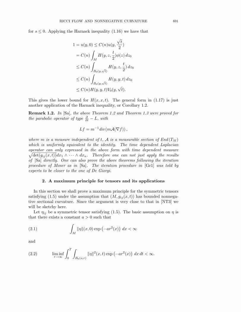
for s ≤ 0. Applying the Harnack inequality (1.16) we have that

1 = u(y, 0) ≤ C(n)u(y,

√t

2)

= C(n)∫

M

H(y, z,t

2)φ(z) dz0

≤ C(n)∫

B0(y,√

t)

H(y, z,t

2) dz0

≤ C(n)∫

B0(y,√

t)

H(y, y, t) dz0

≤ C(n)H(y, y, t)V0(y,√

t).

This gives the lower bound for H(x, x, t). The general form in (1.17) is justanother application of the Harnack inequality, or Corollary 1.2.

Remark 1.2. In [Sa], the above Theorem 1.2 and Theorem 1.3 were proved forthe parabolic operator of type ∂

∂t − L, with

Lf = m−1div (mA(∇f)) ,

where m is a measure independent of t, A is a measurable section of End (TM )which is uniformly equivalent to the identity. The time dependent Laplacianoperator can only expressed in the above form with time dependent measure√

det(gij(x, t))dx1 ∧ · · · ∧ dxn. Therefore one can not just apply the resultsof [Sa] directly. One can also prove the above theorems following the iterationprocedure of Moser as in [Sa]. The iteration procedure in [Gr1] was told byexperts to be closer to the one of De Giorgi.

2. A maximum principle for tensors and its applications

In this section we shall prove a maximum principle for the symmetric tensorssatisfying (1.5) under the assumption that (M, gij(x, t)) has bounded nonnega-tive sectional curvature. Since the argument is very close to that in [NT3] wewill be sketchy here.

Let ηij be a symmetric tensor satisfying (1.5). The basic assumption on η isthat there exists a constant a > 0 such that

(2.1)∫

M

‖η‖(x, 0) exp(−ar2(x)

)dx < ∞

and

(2.2) lim infr→∞

∫ T

0

∫B0(o,r)

‖η‖2(x, t) exp(−ar2(x)

)dx dt < ∞.

892 LEI NI

Here ‖η‖(x, t) is the norm of ηij(x, t) with respect to metrics gij(x, t). ButB0(0, r) is the ball with respect to the initial metric gij(x, 0) and r(x) is thedistance from x to a fixed point o ∈ M with respect to the initial metric. Dueto the fact that the maximum principle for the heat equation does not holdon complete manifolds in general, one needs some growth conditions on thesolutions to make it true. The condition (2.2) is optimal by comparing to theexample given in [J, page 211-213]. The above mentioned classical exampleis a solution to the heat equation on R × [0,∞), which has zero initial data.The violation of the uniqueness implies the failure of the maximum principlefor the sub-solutions. The example has growth, as |x| → ∞, just faster thanexp(ar2(x)). The condition (2.1) is needed to ensure that the equation (1.5)does have a solution indeed. It is also in the sharp form.

Before we state our result, let us first fix some notations. Let ϕ : [0,∞) →[0, 1] be a smooth function so that ϕ ≡ 1 on [0, 1] and ϕ ≡ 0 on [2,∞). For anyx0 ∈ M and R > 0, let ϕx0,R be the function defined by

ϕx0,R(x) = ϕ

(r(x, x0)

R

).

Again, r(x, y) denotes the distance function of the initial metric. Let fx0,R bethe solution of (

∂

∂t− ∆

)f = −f

with initial value ϕx0,R, given by

fx0,R(x, t) =∫

M

H(x, y, t)ϕx0,R(y)dy0.

It is easy to see that f is defined for all t and positive, and it is bounded fort > 0.

We shall establish the following maximum principle.

Theorem 2.1. Let (M, gij(x, t)) be a complete noncompact Riemannian mani-folds satisfying (1.1)–(1.3), with nonnegative sectional curvature. Let η(x, t) be asymmetric tensor satisfying (1.5) on M × [0, T ] with 0 < T < 1

40a such that ||η||satisfies (2.1) and (2.2). Suppose at t = 0, ηij ≥ −bgij(x, 0) for some constantb ≥ 0. Then there exists 0 < T0 < T depending only on T and a so that thefollowing are true.

(i) ηij(x, t) ≥ −be(4n√

A0+1)tgij(x, t) for all (x, t) ∈ M × [0, T0].(ii) For any T0 > t′ ≥ 0, suppose that there is a point x′ in Mm and there ex-

ist constants ν > 0 and R > 0 such that the sum of the first k eigenvaluesλ1, . . . , λk of ηij satisfies

λ1 + · · · + λk ≥ −kb + νkϕx′,R


for all x at time t′. Then for all t > t′ and for all x ∈ M , the sum ofthe first k eigenvalues of ηij(x, t), with respect to gij(x, t), satisfies

λ1 + · · · + λk ≥ −kbe(4n√

A0+1)t + νkfx′,R(x, t − t′).

Proof. We only prove (ii). The proof of (i) is by the exactly same, if not easier,argument. First we let

(2.3) h(x, t) =∫

M

H(x, y, t)‖η‖(y, 0) dy0.

It is easy to see that h(x, t) is a solution to (1.4). Using Corollary 1.2, theassumption (2.2) and the maximum principle of [NT1] we have that

(2.4) exp (−2√

A0t)‖η‖(x, t) ≤ h(x, t).

Denote by A0(o, r1, r2) the annulus B0(o, r2) \ B0(o, r1). Here o ∈ M is a fixedpoint B0(o, r) is the ball as before. For any R > 0, let σR be a cut-off functionwhich is 1 on A0(o, R

4 , 4R) and 0 outside A0(o, R8 , 8R). We define

hR(x, t) =∫

M

H(x, y, t)σR(y)||η||(y, 0)dy0.

Then hR satisfies the heat equation with initial data σR||η||. By Lemma 2.2of [NT3], noticing that the only thing used in Lemma 2.2 is the heat kernelupper bound estimate, we have that there exists a function τ(r) > 0 withlimr→∞ τ(r) = 0 and T0 > 0 such that for all (x, t) ∈ Ao(R

2 , 2R) × [0, T0]

h(x, t) ≤ hR(x, t) + τ(R)

and for any r > 0lim

R→∞sup

B0(o,r)×[0,T0]

hR = 0.

Now lethR(x, t) = exp

((4n

√A0 + 1)t

)(hR(x, t) + τ(R)) .

By (2.4) we have that‖η‖(x, t) ≤ hR(x, t)

for (x, t) ∈ A0(R2 , 2R) × [0, T0]. We can also construct a positive function

φ(x, t) > 0 (using the representation through heat kernel) satisfying the heatequation (

∂

∂t− ∆

)φ = (4n

√A0 + 1)φ.

894 LEI NI

The big coefficient (4n√

A0 + 1) is to dominate the negative input from thetime differentiation of metrics. We can make φ(x, t) ≥ exp(c(r2(x) + 1)) asin [NT2, Lemma 1.1]. Now we prove theorem for the case ν = 1. Let ψ =−f + εφ + hR + exp((4n

√A0 + 1)t)b and

(ηR)ij(x, t) = ηij(x, t) + ψgij(x, t)

where f = fx0,R(x, t) defined right before the statement of the theorem. Itis easy to see that the first k eigenvalues of (ηR)ij(x, 0) is positive due to theassumption and positivity of φ. The functions φ and hR are constructed so thatηR ≥ 0 on ∂B0(o, R) × [0, T0]. Now if the sum of the first k eigenvalues is notnonnegative on B0(o, R) × [0, T0] we can apply the maximum to the first suchinstance, namely to (x0, t0) ∈ B0(o, R) × [0, T0], where the sum of the first k-eigenvalues of ηR reach zero for the first time inside B0(o, R). By choosing thenormal coordinate near x0, such that ηR is diagonal at x0 and the j-th coordinatedirection is the j-th eigen-direction, we have that

0 ≥(

∂

∂t− ∆

) k∑i,j=1

(ηR)ijgij

=

k∑i,j=1

((∂

∂t− ∆

)(ηR)ij

)gij + 2

k∑i,j=1

(ηR)ijRij

≥k∑

i,j=1

[2Ripjqηpq − Ripηpj − Rpjηip +

((∂

∂t− ∆

)ψ

)gij − 2ψRij

]gij .

Observe that under the assumption Rijij ≥ 0, and under the above choice ofthe orthogonal frame such that the tensor ηij is also diagonal at the fixed point(x0, t0) with its eigenvalues λi of η ordered as λ1 ≤ λ2 ≤ · · · ≤ λn. Then we


have that

k∑i,j=1

[2Ripjqηpq − Ripηpj − Rpjηip

]gij

= 2

(k∑

i=1

n∑p=1

Ripipλp −k∑

i=1

Riiλi

)

= 2

(k∑

i=1

n∑p=1

Ripipλp −k∑

i=1

n∑p=1

Ripipλi

)

= 2

k∑i=1

m∑p=k+1

λpRipip −k∑

i=1

m∑p=k+1

Ripipλi

= 2

k∑i=1

m∑p=k+1

Ripip(λp − λi)

≥ 0.

Then we have that

0 ≥ k

[(∂

∂t− ∆

)ψ

]− 2ψ

k∑ij

Rijgij

≥ k[εφ + hR + exp((4n

√A0 + 1)t)b

]> 0.

The contradiction shows that the sum of the first k-eigenvalue for ηR is non-negative on B0(o, R) × [0, T0]. The theorem follows by letting R → ∞ andε → 0.

The similar maximum principle for the scalar heat equations is relatively easyto prove. They also require an assumption as (2.2). The time dependent case wasfirst proved in [NT1] following the original argument for the time-independentcase in [L]. As an application we have the following approximation result oncontinuous convex functions.

Theorem 2.2. Let (M, gij(x, t)) be as above. Let u(x) be a Lipschitz continuousconvex function satisfying

(2.5) |u|(x) ≤ C exp(ar2(x)

)for some positive constants C and a. Let v(x, t) be the solution to the time-dependent heat equation (1.4). There exists T0 > 0 depending only on a andthere exists T0 > T1 > 0 such that the following are true.

(i) For 0 < t ≤ T0, v(·, t) is a smooth convex function (with respect togij(x, t)).

896 LEI NI

(ii) Let

K(x, t) = w ∈ T 1,0x (M)| vij(x, t)wi = 0, for all j

be the null space of vij(x, t). Then for any 0 < t < T1, K(x, t) is adistribution on M . Moreover the distribution is invariant in time as wellas under the parallel translation.

In order to prove the above theorem we need the following approximationresult due to Greene-Wu [GW3, Proposition 2.3].

Lemma 2.1. Let u be a convex function on M . Assume that u is Lipschitz withLipschitz constant 1. For any b > 0, there is a C∞ convex function w such that

(i) |w(x) − w(y)| ≤ r(x, y);(ii) |w − u| ≤ b on M ; and(iii) wij ≥ −bgij on M .

Proof of Theorem 2.2. In order to apply Theorem 2.1 to current theorem oneneeds to verify that ηij = vij(x, t) satisfies the assumption (2.1) and (2.2).Lemma 2.1 provides a smoothing approximation of u, therefore we only needto verify the assumption for smooth u which satisfies uij ≥ −bgij for someb > 0. The Lemma 3.1 of [NT3] can be applied to current situation to servethis purpose. One just needs to observe that (i) of Lemma 3.1 in [NT3] followsfrom the representation formula via the heat kernel, (ii) of Lemma 3.1 in [NT3]only uses nonnegative Ricci and the argument in the proof of (iii) of Lemma 3.1in [NT3] can be transplanted without any changes to the time-dependent heatoperator. After that, one can conclude that vij(x, t) ≥ 0. By Theorem 2.1 onecan easily infer that the null space of vij(x, y) must be of constant rank for somesmall interval [0, T1]. (See also the forth-coming book [Cetc] for the detailedproof of this point.) The fact that it is invariant under the parallel translationfollows exactly same as in [NT3]. The time-invariance of the null space wassketched in [H2]. See also [Ca]. For a clear and rigorous proof please wait andsee [Cetc].

The following is the main result on the structure of solutions to the Ricci flowpreserving the nonnegativity of the sectional curvature.

Theorem 2.3. Let (M, gij(x, t)) be solution to the (1.1) satisfying (1.3) withnonnegative sectional curvature. Denote (M, gij(x, t)) the universal cover of(M, gij(x, t)). Then M splits isometrically as M = N × M1, where N is acompact manifold with nonnegative sectional curvature. M1 is diffeomorphic toR

k. For the metric on M1, obtained by restricting gij(x, t) onto M1 with t > 0,there is a smooth strictly convex exhaustion function on M1. Moreover, the soulof M1 is a point and the soul of M is N × o, if o is a soul of M1.

Proof. By lifting everything to its universal cover we can assume that M issimply-connected. Let B be the Busemann function on M , with respect to the


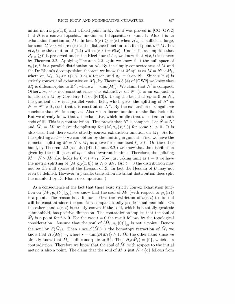
initial metric gij(x, 0) and a fixed point in M . As it was proved in [CG, GW2]that B is a convex Lipschitz function with Lipschitz constant 1. Also it is anexhaustion function on M . In fact B(x) ≥ cr(x) when r(x) is sufficient large,for some C > 0, where r(x) is the distance function to a fixed point o ∈ M . Letv(x, t) be the solution of (1.4) with v(x, 0) = B(x). Under the assumption thatRijij ≥ 0 is preserved under the Ricci flow (1.1), we know that v(x, t) is convexby Theorem 2.2. Applying Theorem 2.2 again we know that the null space ofvij(x, t) is a parallel distribution on M . By the simply-connectedness of M andthe De Rham’s decomposition theorem we know that M splits as M = N ′×M ′

1,where on M1, (vij(x, t)) > 0 as a tensor, and vij ≡ 0 on N ′. Since v(x, t) isstrictly convex and exhaustive on M ′

1, by Theorem 3 (a) of [GW2] we know thatM ′

1 is diffeomorphic to Rk′

, where k′ = dim(M ′1). We claim that N ′ is compact.

Otherwise, v is not constant since v is exhaustive on N ′ (v is an exhaustionfunction on M by Corollary 1.4 of [NT3]). Using the fact that vij ≡ 0 on N ′,the gradient of v is a parallel vector field, which gives the splitting of N ′ asN ′ = N ′′ × R, such that v is constant on N ′′. By the exhaustion of v again weconclude that N ′′ is compact. Also v is a linear function on the flat factor R.But we already know that v is exhaustive, which implies that v → +∞ on bothends of R. This is a contradiction. This proves that N ′ is compact. Let N = N ′

and M1 = M ′1 we have the splitting for (M, gij(x, t1)) for some t1 > 0. It is

also clear that there exists strictly convex exhaustion function on M1. As forthe splitting at t = 0 we can obtain by the limiting argument. First we have theisometric splitting M = N × M1 as above for some fixed t1 > 0. On the otherhand, by Theorem 2.2 (see also [H2, Lemma 8.2]) we know that the distributiongiven by the null space of vij is also invariant in time. Therefore, the splittingM = N × M1 also holds for 0 < t ≤ t1. Now just taking limit as t → 0 we havethe metric splitting of (M, gij(x, 0)) as N × M1. (At t = 0 the distribution maynot be the null spaces of the Hessian of B. In fact the Hessian of B may noteven be defined. However, a parallel translation invariant distribution does splitthe manifold by De Rham decomposition.)

As a consequence of the fact that there exist strictly convex exhaustion func-tion on (M1, gij(t1)|M1

), we know that the soul of M1 (with respect to gij(t1))is a point. The reason is as follows. First the restriction of v(x, t) to its soulwill be constant since the soul is a compact totally geodesic submanifold. Onthe other hand v(x, t) is strictly convex if the soul, which is a totally geodesicsubmanifold, has positive dimension. The contradiction implies that the soul ofM1 is a point for t > 0. For the case t = 0 the result follows by the topologicalconsideration. Assume that the soul of (M1, gij(0))|M1

is not a point. Denotethe soul by S(M1). Then since S(M1) is the homotopy retraction of M1 weknow that Hs(M1) =, where s = dim(S(M1)) ≥ 1. On the other hand since wealready know that M1 is diffeomorphic to R

k. Thus Hs(M1) = 0, which is acontradiction. Therefore we know that the soul of M1 with respect to the initialmetric is also a point. The claim that the soul of M is just N ×o follows from

898 LEI NI

the following simple lemma.

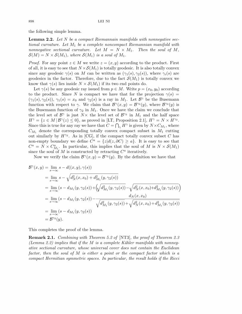
Lemma 2.2. Let N be a compact Riemannain manifolds with nonnegative sec-tional curvature. Let M1 be a complete noncompact Riemannian manifold withnonnegative sectional curvature. Let M = N × M1. Then the soul of M ,S(M) = N × S(M1), where S(M1) is a soul of M1.

Proof. For any point z ∈ M we write z = (x, y) according to the product. Firstof all, it is easy to see that N×S(M1) is totally geodesic. It is also totally convexsince any geodesic γ(s) on M can be written as (γ1(s), γ2(s)), where γi(s) aregeodesics in the factor. Therefore, due to the fact S(M1) is totally convex weknow that γ(s) lies inside N × S(M1) if its two end points do.

Let γ(s) be any geodesic ray issued from p ∈ M . Write p = (x0, y0) accordingto the product. Since N is compact we have that for the projection γ(s) =(γ1(s), γ2(s)), γ1(s) = x0 and γ2(s) is a ray in M1. Let Bγ be the Busemannfunction with respect to γ. We claim that Bγ(x, y) = Bγ2(y), where Bγ2(y) isthe Busemann function of γ2 in M1. Once we have the claim we conclude thatthe level set of Bγ is just N× the level set of Bγ2 in M1 and the half spaceHγ = z ∈ M | Bγ(z) ≤ 0, as proved in [LT, Proposition 2.1], Hγ = N × Hγ2 .Since this is true for any ray we have that C =

⋂γ Hγ is given by N×CM1 , where

CM1 denote the corresponding totally convex compact subset in M1 cuttingout similarly by Hγ2 . As in [CG], if the compact totally convex subset C hasnon-empty boundary we define Ca = z|d(z, ∂C) ≥ a. It is easy to see thatCa = N × Ca

M1. In particular, this implies that the soul of M is N × S(M1)

since the soul of M is constructed by retracting Ca iteratively.Now we verify the claim Bγ(x, y) = Bγ2(y). By the definition we have that

Bγ(x, y) = lims→∞

s − d((x, y), γ(s))

= lims→∞

s −√

d2N (x, x0) + d2

M1(y, γ2(s))

= lims→∞

(s − dM1(y, γ2(s))+(√

d2M1

(y, γ2(s))−√

d2N (x, x0)+d2

M1(y, γ2(s))

)= lim

s→∞(s − dM1(y, γ2(s))−

dN (x, x0)√d2

M1(y, γ2(s))+

√d2

N (x, x0)+d2M1

(y, γ2(s))

= lims→∞

(s − dM1(y, γ2(s))

= Bγ2(y).

This completes the proof of the lemma.

Remark 2.1. Combining with Theorem 5.2 of [NT3], the proof of Theorem 2.3(Lemma 2.2) implies that if the M is a complete Kahler manifolds with nonneg-ative sectional curvature, whose universal cover does not contain the Euclideanfactor, then the soul of M is either a point or the compact factor which is acompact Hermitian symmetric spaces. In particular, the result holds if the Ricci


curvature of M is positive somewhere. Therefore one can view the result such asTheorem 4.2 or Theorem 5.1 as a complex analogue of the ‘soul theorem’ whenonly the nonnegativity of the bisectional curvature is assumed.

Since the Ricci flow preserves the nonnegativity of the curvature operator(if the curvature is uniformly bounded by [H2]) we have the following corol-lary on the structure of complete simply-connected Riemannian manifolds withnonnegative curvature operator.

Corollary 2.1. Let M be a complete simply-connected Riemannian manifoldwith bounded nonnegative curvature operator. Then M is a product of a com-pact Riemannian manifold with nonnegative curvature operator with a completenoncompact manfold which is diffeomorphic to R

k.

Remark 2.2. The compact factor in the above result has been classified in [CY]to be the product of compact symmetric spaces, Kahler manifolds biholomorphicto the complex projective spaces and the manifolds homeomorphic to spheres.See also [CC] and [GaM]. More importantly, it relies crucially on the result of[H2], [MM] and [SiY]. Some literature attribute the result to [GM]. But [GM]just proved the cohomology groups with coefficient R (of compact Mn with non-negative curvature operator) are the same as the sphere Sn. It seems that theclassification was quite far from finished without the crucial later work in [MM]and [SiY].

The above Corollary 2.1 was proved earlier in [N] by Noronha without assum-ing the curvature tensor being bounded. Our method here has this restrictionon boundedness of the curvature since we have to use the short time existenceresult of Shi in [Sh2] on the Ricci flow. In the case of dimension three, the sameresult holds if one assumes that the sectional curvature is nonnegative, which issame as the curvature operator being nonnegative. However in [Sh1] the strongerresult was proved even for nonnegative Ricci curvature case. The proof in [Sh1]appeals to the previous deep results of Hamilton [H1, H2] and Schoen-Yau [SY].

3. Examples

As another application of Theorem 2.3 we give examples of complete Rie-mannian manifolds with nonnegative sectional curvature on which the Ricciflow (at least the solution satisfying (1.3)) does not preserve the nonnegativityof the sectional curvature. These manifolds can be constructed as follows. LetG = SO(n + 1) with the standard bi-invariant metric and H = SO(n) be itsclose subgroup. Then H has action on G (as translation) as well as its standardaction on P = R

n (as rotation). Let M = G×P/H. Topologically M is just thetangent bundle over Sn since H → G → G/H = Sn is just the correspondingprinciple bundle over Sn. The construction is due to Cheeger and Gromoll [CG]where the examples were to illustrate their structure theorem therein. Aboutthese examples the following are known (cf. [CG]): The metric on M has non-negative sectional curvature due to the fact that the metric is constructed as the

900 LEI NI

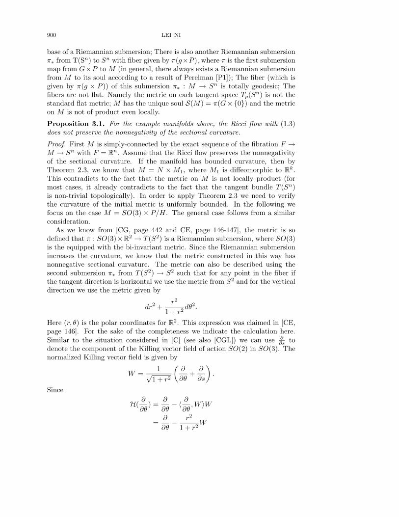
base of a Riemannian submersion; There is also another Riemannian submersionπ∗ from T(Sn) to Sn with fiber given by π(g×P ), where π is the first submersionmap from G×P to M (in general, there always exists a Riemannian submersionfrom M to its soul according to a result of Perelman [P1]); The fiber (which isgiven by π(g × P )) of this submersion π∗ : M → Sn is totally geodesic; Thefibers are not flat. Namely the metric on each tangent space Tp(Sn) is not thestandard flat metric; M has the unique soul S(M) = π(G×0) and the metricon M is not of product even locally.

Proposition 3.1. For the example manifolds above, the Ricci flow with (1.3)does not preserve the nonnegativity of the sectional curvature.

Proof. First M is simply-connected by the exact sequence of the fibration F →M → Sn with F = R

n. Assume that the Ricci flow preserves the nonnegativityof the sectional curvature. If the manifold has bounded curvature, then byTheorem 2.3, we know that M = N × M1, where M1 is diffeomorphic to R

k.This contradicts to the fact that the metric on M is not locally product (formost cases, it already contradicts to the fact that the tangent bundle T (Sn)is non-trivial topologically). In order to apply Theorem 2.3 we need to verifythe curvature of the initial metric is uniformly bounded. In the following wefocus on the case M = SO(3) × P/H. The general case follows from a similarconsideration.

As we know from [CG, page 442 and CE, page 146-147], the metric is sodefined that π : SO(3)×R

2 → T (S2) is a Riemannian submersion, where SO(3)is the equipped with the bi-invariant metric. Since the Riemannian submersionincreases the curvature, we know that the metric constructed in this way hasnonnegative sectional curvature. The metric can also be described using thesecond submersion π∗ from T (S2) → S2 such that for any point in the fiber ifthe tangent direction is horizontal we use the metric from S2 and for the verticaldirection we use the metric given by

dr2 +r2

1 + r2dθ2.

Here (r, θ) is the polar coordinates for R2. This expression was claimed in [CE,

page 146]. For the sake of the completeness we indicate the calculation here.Similar to the situation considered in [C] (see also [CGL]) we can use ∂

∂s todenote the component of the Killing vector field of action SO(2) in SO(3). Thenormalized Killing vector field is given by

W =1√

1 + r2

(∂

∂θ+

∂

∂s

).

Since

H(∂

∂θ) =

∂

∂θ− 〈 ∂

∂θ, W 〉W

=∂

∂θ− r2

1 + r2W


the metric on the base of ∂∂θ is given by

‖ ∂

∂θ‖2

M = ‖H(∂

∂θ)‖2 =

r2

1 + r2.

Here H( ∂∂θ ) denotes the horizontal lift (projection) of ∂

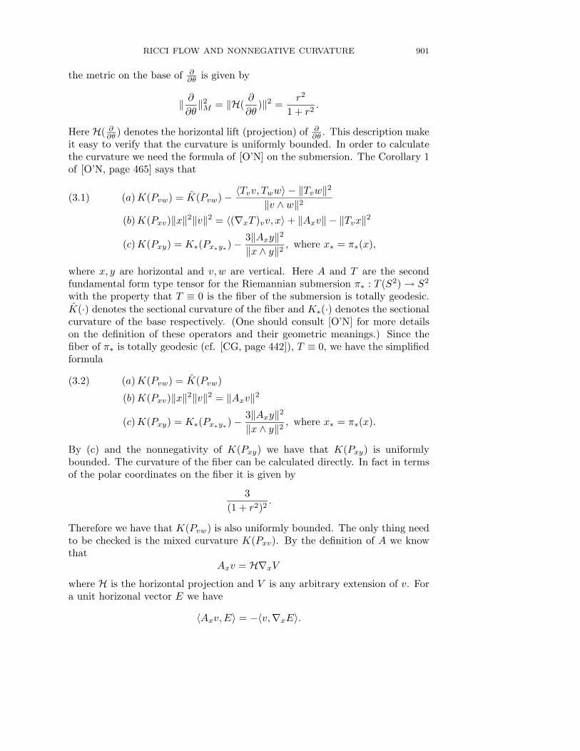
∂θ . This description makeit easy to verify that the curvature is uniformly bounded. In order to calculatethe curvature we need the formula of [O’N] on the submersion. The Corollary 1of [O’N, page 465] says that

(a)K(Pvw) = K(Pvw) − 〈Tvv, Tww〉 − ‖Tvw‖2

‖v ∧ w‖2

(b)K(Pxv)‖x‖2‖v‖2 = 〈(∇xT )vv, x〉 + ‖Axv‖ − ‖Tvx‖2

(c)K(Pxy) = K∗(Px∗y∗) −3‖Axy‖2

‖x ∧ y‖2, where x∗ = π∗(x),

(3.1)

where x, y are horizontal and v, w are vertical. Here A and T are the secondfundamental form type tensor for the Riemannian submersion π∗ : T (S2) → S2

with the property that T ≡ 0 is the fiber of the submersion is totally geodesic.K(·) denotes the sectional curvature of the fiber and K∗(·) denotes the sectionalcurvature of the base respectively. (One should consult [O’N] for more detailson the definition of these operators and their geometric meanings.) Since thefiber of π∗ is totally geodesic (cf. [CG, page 442]), T ≡ 0, we have the simplifiedformula

(a)K(Pvw) = K(Pvw)

(b)K(Pxv)‖x‖2‖v‖2 = ‖Axv‖2

(c)K(Pxy) = K∗(Px∗y∗) −3‖Axy‖2

‖x ∧ y‖2, where x∗ = π∗(x).

(3.2)

By (c) and the nonnegativity of K(Pxy) we have that K(Pxy) is uniformlybounded. The curvature of the fiber can be calculated directly. In fact in termsof the polar coordinates on the fiber it is given by

3(1 + r2)2

.

Therefore we have that K(Pvw) is also uniformly bounded. The only thing needto be checked is the mixed curvature K(Pxv). By the definition of A we knowthat

Axv = H∇xV

where H is the horizontal projection and V is any arbitrary extension of v. Fora unit horizonal vector E we have

〈Axv, E〉 = −〈v,∇xE〉.

902 LEI NI

Therefore it is enough to show that the right hand side is bounded. Since, bythe first submersion consideration using the quotient, we know that K(Pxy) isnonnegative. Therefore by (c) of (3.2),

‖Axy‖2 ≤ 13K∗(Px∗y∗)‖x ∧ y‖2.

This shows that |〈v,∇xE〉| is uniformly bounded.For the sake of the completeness we also include a proof of the fact that the

fiber of π∗ is totally geodesic since there is no written proof in the literature.Recall that M = SO(n+1)×P/SO(n). Here SO(n) is viewed as close subgroupof SO(n + 1) by the inclusion:

A →(

1 00 A

).

We have the involution ζ which is given by

ζ =(

1 00 −I

).

ζ acts on SO(n+1) by A → ζAζ. It is easy to see that the fixed point set of ζ isSO(n). Now we consider the action of ζ on SO(n + 1)× P as (g, x) → (ζgζ, x).It is easy to see that this action is commutative with the action of SO(n) sincefor any h ∈ SO(n) ζh = hζ. Therefore the action descends to M . It is easy tosee that the fixed point of this action is π(e, P ). This implies that the fiber (ofthe submersion π∗) π(e, P ) is totally geodesic since it is the fixed point set ofan isometry. The other fiber can be verified similarly since for any point p ∈ Sn

there is also an involution fixes p.

Remark 3.1. Since we used Theorem 2.3 in Proposition 3.1 above, the examplesonly apply to the solution to Ricci flow satisfying (1.3). This includes the solutionprovided by Shi’s existence theorem. It is still unknown that the solution to Ricciflow satisfying (1.3) is unique or not. Whether or not there exist similar compactexamples also worths further investigation.

Acknowledgement

The author would like to thank Professors Ben Chow, Peter Li, Miles Simon,H. Wu and S.-T. Yau for their interests in this work. Discussions with ProfessorsTom Ilmanen and Jiaping Wang are very helpful. We would like to thank themtoo. Special thanks go to Professor Luen-Fai Tam for many helpful suggestions.The paper is not possible without the previous collaboration [NT3] with him.Finally we would like to thank the referee for her/his helpful comments.


References

[AC] G. Anderson and B. Chow, A pinching estimate for solutions of linearized Ricciflow system on 3-manifolds, to appear in Calculus Variation and PDE.

[B] S. Bando, On classification of three-dimensional compact Kahler manifolds ofnonnegative bisectional curvature, J. Differential Geom. 19 (1984), 283–297.

[Ca] H.-D. Cao, On dimension reduction in the Kahler-Ricci flow, Comm. Anal. Geom.12 (2004), 305–320.

[CC] H.-D. Cao and B. Chow, Compact Kahler manifolds with nonnegative curvatureoperator, Invent. Math. 83 (1986), 553–556.

[C] J. Cheeger, Some examples of manifolds of nonnegative curvature, J. DifferentialGeom. 8 (1972), 623-628.

[CE] J. Cheeger and D. Ebin, Comparison theorems in Riemannian geometry, North-Holland, Amsterdam, 1975.

[CG] J. Cheeger and D. Gromoll, On the structure of complete manifolds of nonnegativecurvature, Ann. of Math. 96 (1972), 413–443.

[Cetc] B. Chow and others, The Ricci flow: techniques and applications, in preparation.

[Ch] B. Chow, A Survey of Hamilton’s Program for the Ricci Flow on 3-manifolds,preprint, arXiv: math.DG/ 0211266.

[CGL] B. Chow, David Glickenstein and Peng Lu, Metric transformations under collaps-ing of Riemannian manifolds, Math. Res. Lett. 10 (2003), 737-746.

[CH] B. Chow and R. Hamilton, Constrained and linear Harnack inqualities for para-bolic equations, Invent. Math. 129 (1997), 213–238.

[CY] B. Chow and Deane Yang, Rigidity of nonnegatively curved compact quaternionic-Kahler manifolds, J. Differential Geom. 29 (1989), 361–372.

[GaM] S. Gallot and D. Meyer, Operateur de courbure et Laplacian des formes differen-tielles d’une variete Riemanniene, J. Math. Pures Appl. 54 (1975), 285–304.

[GW1] R. E. Greene and H. Wu, Integrals of subharmonic functions on manifolds ofnonnegative curvature, Invent. Math. 27 (1974), 265–298.

[GW2] , C∞ convex function and the manifolds of positive curvature, Acta. Math.137 (1976), 209–245.

[GW3] , C∞ approximations of convex, subharmonic, and plurisubharmonic func-

tions, Ann. Scient. Ec. Norm. Sup. 12 (1979), 47–84.

[Gr1] A. Grigor’yan, The heat equation on noncompact Riemannian manifolds, Math.USSR Sbornik 72 (1992), 47–77.

[Gr2] , Guassian upper bounds for the heat kernel on arbitrary manifolds, J.Differential Geom. 45 (1997), 33–52.

[Gu] C. Guenther, The fundamental solution on manifolds with time-dependent met-rics, J. Geom. Anal. 12 (2002), 425–436.

[H1] R. S. Hamilton, Three-manifolds with positive Ricci curvature, J. DifferentialGeom. 17 (1982), 255–306.

[H2] , Four-manifolds with positive curvature operator, J. Differential Geom.24 (1986), 153–179.

[H3] , The Harnack estimate for the Ricci flow, J. Differential Geom. 37 (1993),225–243.

[J] F. John, Partial Differential Equations, fourth edition, Springer-Verlag, NewYork, 1982.

[L] P. Li, Lectures on heat equations, 1991-1992 at UCI.

[LT] P. Li and L.-F. Tam, Positive harmonic functions on complete manifolds withnon-negative curvature outside a compact set, Ann. of Math. 125 (1987), 171–207.

[LY] P. Li and S.-T. Yau, On the parabolic kernel of the Schrodinger operator, ActaMath. 156 (1986), 139–168.

904 LEI NI

[MM] M. Micallef and D. Moore, Minimal two-spheres and the topology of manifoldswith positive curvature on totally isotropic two-planes, Ann. of Math. (2) 127(1988), 199–227.

[M] N. Mok, The uniformization theorem for compact Kahler manifolds of nonnega-tive holomorphic bisectional curvature, J. Differential Geom. 27 (1988), 179–214.

[Mo] J. Moser, A Harnack inequality for parabolic differential equations, Comm. PureAppl. Math. 17 (1964), 101–134.

[N] M. Noronha, A splitting theorem for complete manifolds with nonnegative curva-ture operator, Proceedings of AMS. 105 (1989), 979–985.

[NT1] L. Ni and L.-F.Tam, Kahler Ricci flow and Poincare-Lelong equation, Comm.Anal. Geom. 12 (2004), 111–141.

[NT2] , Plurisubharmonic functions and the Kahler-Ricci flow, Amer. J. Math.125 (2003), 623–645.

[NT3] , Plurisubharmonic functions and the structure of complete Kahler mani-folds with nonnegative curvature, J. Differential Geom. 64 (2003), 457–524.

[O’N] B. O’Neill, The fundamental equations of a submersion, Michigan Math. J. 13(1966), 459–469.

[P1] G. Perelman, Proof of the soul conjecture of Cheeger and Gromoll, J. DifferentialGeom. 40 (1994), 209–212.

[P2] , The entropy formula for the Ricci flow and its geometric applications,arXiv: math.DG/ 0211159.

[Sa] L. Saloff-Coste, Uniformly elliptic operators on Riemannian manifolds, J. Differ-ential Geom. 36 (1992), 417–450.

[SY] R. Schoen and S.- T. Yau, Complete three-dimensional manifolds with positiveRicci curvature and scalar curvature,, Seminar on Differential Geometry, Ann. ofMath. Stud., 102, 209–228, Princeton Univ. Press, Princeton, N.J., 1982.

[Sh1] W. X. Shi, Complete noncompact three-manifolds with nonnegative Ricci curva-ture, J. Differential Geom. 29 (1989), 353–360.

[Sh2] , Deforming the metric on complete Riemannian manifolds, J. DifferentialGeom. 30 (1989), 223–301.

[Sh3] , Ricci flow and the uniformization on complete noncompact Kahler man-ifolds, J. Differential Geom. 45 (1997), 94–220.

[SiY] Y.-T. Siu and S.-T. Yau, Compact Kahler manifolds of positive bisectional cur-vature, Invent. Math. 59 (1980), 189–204..

[W] H. Wu, An elementary methods in the study of nonnegative curvature, Acta.Math. 142 (1979), 57–78.

Department of Mathematics, University of California, San Diego, La Jolla, CA92093

E-mail address: [email protected]

Ricci flow and nonnegativity of sectional curvature

Documents

Transcript of Ricci flow and nonnegativity of sectional curvature