Available online at www.sciencedirect.com

ScienceDirect

Nuclear Physics B 895 (2015) 33–63

www.elsevier.com/locate/nuclphysb

RG-Whitham dynamics and complex

Hamiltonian systems

A. Gorsky a,b, A. Milekhin a,b,c,∗

a Institute for Information Transmission Problems, B. Karetnyi 15, Moscow 127051, Russiab Moscow Institute of Physics and Technology, Dolgoprudny 141700, Russia

c Institute for Theoretical and Experimental Physics, B. Cheryomushkinskaya 25, Moscow 117218, Russia

Received 4 March 2015; accepted 28 March 2015

Available online 1 April 2015

Editor: Herman Verlinde

Abstract

Inspired by the Seiberg–Witten exact solution, we consider some aspects of the Hamiltonian dynamics with the complexified phase space focusing at the renormalization group (RG)-like Whitham behavior. We show that at the Argyres–Douglas (AD) point the number of degrees of freedom in Hamiltonian system effectively reduces and argue that anomalous dimensions at AD point coincide with the Berry indexes in classical mechanics. In the framework of Whitham dynamics AD point turns out to be a fixed point. We demonstrate that recently discovered Dunne–Ünsal relation in quantum mechanics relevant for the exact quantization condition exactly coincides with the Whitham equation of motion in the �-deformed theory.© 2015 The Authors. Published by Elsevier B.V. This is an open access article under the CC BY license (http://creativecommons.org/licenses/by/4.0/). Funded by SCOAP3.

1. Introduction

The holomorphic and complex Hamiltonian systems attract now the substantial interest par-tially motivated by their appearance in the Seiberg–Witten solution to the N = 2 SUSY YM theories [1]. They have some essential differences in comparison with the real case mainly due to the nontrivial topology of the fixed energy Riemann surfaces in the phase space. Another subtle issue concerns the choice of the quantization condition which is not unique.

* Corresponding author.E-mail addresses: gorsky@itep.ru (A. Gorsky), milekhin@itep.ru (A. Milekhin).

http://dx.doi.org/10.1016/j.nuclphysb.2015.03.0280550-3213/© 2015 The Authors. Published by Elsevier B.V. This is an open access article under the CC BY license (http://creativecommons.org/licenses/by/4.0/). Funded by SCOAP3.

34 A. Gorsky, A. Milekhin / Nuclear Physics B 895 (2015) 33–63

The very idea of our consideration is simple – to use some physical intuition developed in the framework of the SUSY gauge theories and apply it back to complex or holomorphic Hamil-tonian systems which are under the carpet. The nontrivial phenomena at the gauge side have interesting manifestations in the dynamical systems with finite number degrees of freedom. There are a few different dynamical systems in SUSY gauge theory framework. In the N = 2 case one can define a pair of the dynamical systems related to each other in a well defined manner (see [2]for review). The second Whitham-like Hamiltonian system [3] is defined on the moduli space of the first Hamiltonian system. Note that there is no need for the first system to be integrable while the Whitham system is certainly integrable. It can be considered as the RG flow in the field theory framework [4].

One more dynamical system can be defined upon the deformation to N = 1 SUSY where the chiral ring relation plays the role of its energy level. In this case one deals with the Dijkgraaf–Vafa matrix model [5,6] in the large N limit. It is known that matrix models in the large N limit give rise to one-dimensional mechanical system, with the loop equation playing the role of energy conservation and 1-point resolvent playing the role of action differential pdq . The degrees of freedom in all cases can be attributed to the brane coordinates in the different dimensions and mutual coexistence of the dynamical systems plays the role of the consistency condition of the whole brane configuration. We shall not use heavily the SUSY results but restrict ourselves only by application of a few important issues inherited from the gauge theory side to the Hamiltonian systems with the finite number degrees of freedom. Namely we shall investigate the role of the RG-flows, anomalous dimensions at AD points and condensates in the context of the classical and quantum mechanics.

First we shall focus at the behavior of the dynamical system near the AD point. It is inter-esting due to the following reason. It was shown in [7] that the AD point in the softly broken N = 2 theory corresponds to the point in the parameter space where the deconfinement phase transition occurs. The field theory analysis is performed into two steps. First the AD point at the moduli space of N = 2 SUSY YM theory gets identified and than the vanishing of the monopole condensate which is the order parameter is proved upon the perturbation. The consideration in the complex classical mechanics is parallel to the field theory therefore the first step involves the explanation of the AD point before any perturbation. We argue that the number of degrees of freedom at AD point gets effectively reduced which is the key feature of the AD point in classical mechanics. Moreover we can identify the analog of the critical indices at AD point in Hamiltonian system as the Berry indexes relevant for the critical behavior near caustics. Also, we propose a definition for a “correlation length” for a mechanical system so that correspond-ing anomalous dimensions coincide with the field-theoretical ones. From the Whitham evolution viewpoint the AD point is the fixed point. However the second step concerning the perturbation and identification of the condensates is more complicated and we shall restrict ourselves by the few conjectures. Note that the previous discussion of the Hamiltonian interpretation of the AD points can be found in [8] however that paper was focused at another aspects of the problem.

Quantization of complex quantum mechanical systems is more subtle and we consider the role of the Whitham dynamics in this problem. The progress in this direction concerns the attempt to formulate the exact energy quantization condition which involves the non-perturbative instanton corrections. It turns out that at least in the simplest examples [9] the exact quantization condition involves only two functions. Later the relation between these two functions has been found [10]. We shall argue that the Dunne–Ünsal relation [10] which supplements the Jentschura–Zinn-Justin quantization condition [9] can be identified as the equation of motion in the Whitham theory.

A. Gorsky, A. Milekhin / Nuclear Physics B 895 (2015) 33–63 35

To this end we derive the Whitham equations in the presence of �-deformation, which has not been done in a literature before.

The paper is organized as follows. Whitham dynamics is briefly reviewed in Section 2. In Section 3 we shall consider the different aspects of the AD points in the classical mechan-ics. Section 4 is devoted to the clarification of the role of the Dunne–Ünsal relation and to the derivation of Whitham equations in the �-deformed theory. Also, we discuss various quantiza-tion conditions for complex systems and elucidate the role of the curve of marginal stability. The key findings of the paper are summarized in the Conclusion. In Appendix A we show how the Bethe ansatz equations are modified by the higher Whitham times.

2. Whitham hierarchy

2.1. Generalities

Let us define some notations which will be used later, for a nice review see [11]. Hyper-elliptic curve is defined by

y2 = P2N(x) (2.1)

where P2N(x) – is polynomial of degree 2N – below, we will be mostly concerned with this particular case. There are 2g = 2N − 2 cycles Ai , Bi , i = 1, . . . , g which can be chosen as follows (Ai, Aj) = 0, (Bi, Bj ) = 0, (Ai, Bj ) = δij . For genus g hyper-elliptic curve there are exactly g holomorphic abelian-differentials of the first kind ωk :∮

Aj

ωk = δjk (2.2)

which are linear combinations of dx/y, . . . , xg−1dx/y. Period matrix is given by:∮Bj

ωk = τjk (2.3)

Define d�j -meromorphic abelian differential of the second-kind by the following require-ments:

normalization:∮Ak

d�j = 0 (2.4)

and behavior near some point (puncture):

d�j ≈ (ξ−j−1 + O(1))dξ, ξ → 0 (2.5)

d�0 is actually abelian differential of the third kind – with two simple poles with residues +1, −1.

Below we will use Riemann bilinear identity for the pair of meromorphic differentials ω1, ω2:

g∑j=1

⎛⎜⎝∮

A

ω1

∮B

ω2 −∮B

ω1

∮A

ω2

⎞⎟⎠ = 2πi

∑poles

(d−1ω1)ω2 (2.6)

j j j j

36 A. Gorsky, A. Milekhin / Nuclear Physics B 895 (2015) 33–63

however sometimes it is more convenient to work with non-normalized differentials dvk =xkdx/y:

ωkl =∮Al

dvk (2.7)

ωDlk =

∮Bl

dvk (2.8)

Recall now some general facts concerning Whitham dynamics. In classical mechanics, action variables ai are independent of time. However, sometimes it is interesting to consider a bit dif-ferent situation when some parameters of the system become adiabatically dependent on times. Then the well-known adiabatic theorem states that unlike other possible integrals of motion, ai are still independent (with exponential accuracy) on times.

While considering finite-gap solutions to the integrable system one deals with a spectral curve and a tau-function

τ = θ(∑j

tj �U(j)), (2.9)

θ(z|τ) – is a conventional theta-function,

θ(�z|τ) =∑

�kexp((�z, �k) + πi(�k, τ �k)) (2.10)

If one introduces “slow” (Whitham) times ti = εTi, ε → 0, Whitham hierarchy equations tell us how moduli can be slowly varied provided (2.9) still gives the solution to the leading order in ε [12,3]. These equations have zero-curvature form [3]

∂d�i

∂Tj

= ∂d�j

∂Ti

(2.11)

This guarantees the existence of dS such that

∂dS

∂Ti

= d�i (2.12)

which results in the adiabatic theorem:

∂ai

∂Tj

= 0 (2.13)

The full Whitham–Krichever hierarchy (2.11) has a variety of solutions. Every dS satisfy-ing (2.12) generates some solution.

Here we have to stop and make one comment concerning the closed Toda chain-case. The Hamiltonian is given by

H =N+1∑i=1

p2i

2+ �

∑i

exp(qi − qi+1), qi+N = qi (2.14)

The spectral curve equation for N -particle chain reads as

y2 = P 2 (x) − 4�2N (2.15)

N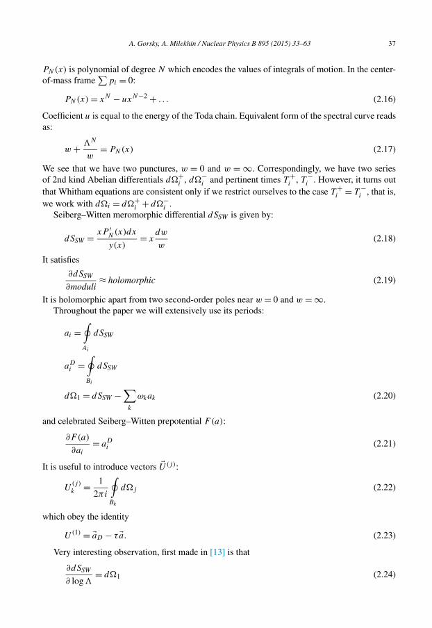

A. Gorsky, A. Milekhin / Nuclear Physics B 895 (2015) 33–63 37

PN(x) is polynomial of degree N which encodes the values of integrals of motion. In the center-of-mass frame

∑pi = 0:

PN(x) = xN − uxN−2 + . . . (2.16)

Coefficient u is equal to the energy of the Toda chain. Equivalent form of the spectral curve reads as:

w + �N

w= PN(x) (2.17)

We see that we have two punctures, w = 0 and w = ∞. Correspondingly, we have two series of 2nd kind Abelian differentials d�+

i , d�−i and pertinent times T +

i , T −i . However, it turns out

that Whitham equations are consistent only if we restrict ourselves to the case T +i = T −

i , that is, we work with d�i = d�+

i + d�−i .

Seiberg–Witten meromorphic differential dSSW is given by:

dSSW = xP ′N(x)dx

y(x)= x

dw

w(2.18)

It satisfies

∂dSSW

∂moduli≈ holomorphic (2.19)

It is holomorphic apart from two second-order poles near w = 0 and w = ∞.Throughout the paper we will extensively use its periods:

ai =∮Ai

dSSW

aDi =

∮Bi

dSSW

d�1 = dSSW −∑

k

ωkak (2.20)

and celebrated Seiberg–Witten prepotential F(a):

∂F (a)

∂ai

= aDi (2.21)

It is useful to introduce vectors �U(j):

U(j)k = 1

2πi

∮Bk

d�j (2.22)

which obey the identity

U(1) = �aD − τ �a. (2.23)

Very interesting observation, first made in [13] is that

∂dSSW = d�1 (2.24)

∂ log�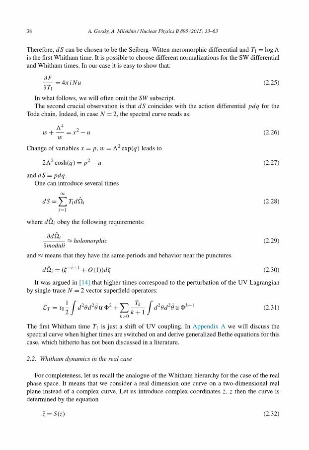

38 A. Gorsky, A. Milekhin / Nuclear Physics B 895 (2015) 33–63

Therefore, dS can be chosen to be the Seiberg–Witten meromorphic differential and T1 = log�

is the first Whitham time. It is possible to choose different normalizations for the SW differential and Whitham times. In our case it is easy to show that:

∂F

∂T1= 4πiNu (2.25)

In what follows, we will often omit the SW subscript.The second crucial observation is that dS coincides with the action differential pdq for the

Toda chain. Indeed, in case N = 2, the spectral curve reads as:

w + �4

w= x2 − u (2.26)

Change of variables x = p, w = �2 exp(q) leads to

2�2 cosh(q) = p2 − u (2.27)

and dS = pdq .One can introduce several times

dS =∞∑i=1

Tid�i (2.28)

where d�i obey the following requirements:

∂d�i

∂moduli≈ holomorphic (2.29)

and ≈ means that they have the same periods and behavior near the punctures

d�i = (ξ−i−1 + O(1))dξ (2.30)

It was argued in [14] that higher times correspond to the perturbation of the UV Lagrangian by single-trace N = 2 vector superfield operators:

LT = τ01

2

∫d2θd2θ tr�2 +

∑k>0

Tk

k + 1

∫d2θd2θ tr�k+1 (2.31)

The first Whitham time T1 is just a shift of UV coupling. In Appendix A we will discuss the spectral curve when higher times are switched on and derive generalized Bethe equations for this case, which hitherto has not been discussed in a literature.

2.2. Whitham dynamics in the real case

For completeness, let us recall the analogue of the Whitham hierarchy for the case of the real phase space. It means that we consider a real dimension one curve on a two-dimensional real plane instead of a complex curve. Let us introduce complex coordinates z, z then the curve is determined by the equation

z = S(z) (2.32)

A. Gorsky, A. Milekhin / Nuclear Physics B 895 (2015) 33–63 39

We shall assume that z, z pair yields the phase space of some dynamical system and the curve itself corresponds to its energy level. With this setup it is clear that Poisson bracket between zand z is fixed by the standard symplectic form:

{z, z} = 1 (2.33)

Let us remind the key points from [15] where the Whitham hierarchy for the plane curve was developed. The phase space interpretation has been suggested in [16]. The Schwarz function S(z)

is assumed to be analytic in a domain including the curve. Consider the map of the exterior of the curve to the exterior of the unit disk

ω(z) = z

r+

∑j

pj z−j (2.34)

where ω is defined on the unit circle. Introduce the moments of the curve

tn = 1

2πin

∮z−nS(z)dz, n < 0 (2.35)

t0 = 1

2πi

∮S(z)dz (2.36)

vn = 1

2πi

∮znS(z)dz, n > 0 (2.37)

v0 =∮

log |z|dz (2.38)

which provide the following expansion for the Schwarz function

S(z) =∑

ktkzk−1 + t0z

−1 +∑

kvkz−k−1 (2.39)

Let us define the generating function

S(z) = ∂z�(z) (2.40)

where

�(z) =∑k=1

tkzk + t0 log z −

∑k=1

vkz−kk−1 − 1/2v0. (2.41)

One can derive the following relations

∂t0�(z) = logω(z) (2.42)

∂tn�(z) = (zn(ω))+ + 1/2(zn(ω))0 (2.43)

∂tn�(z) = (Sn(ω))+ + 1/2(Sn(ω))0 (2.44)

Therefore we identify logω as angle variable and the area inside the curve t0 as the action vari-able. Let us denote by (S(ω))+ the truncated Laurent series with only positive powers of ω kept and the (S(ω))0 is the constant term in the series. The differential d�

d� = Sdz + logωdt0 +∑

(Hkdtk − Hkdtk) (2.45)

yields the Hamiltonians and � itself can be immediately identified as the generating function for the canonical transformation from the pair (z, z) to the canonical pair (t0, logω).

40 A. Gorsky, A. Milekhin / Nuclear Physics B 895 (2015) 33–63

The dynamical equations read

∂tnS(z) = ∂zHn(z) (2.46)

∂tnS(z) = ∂zHn(z) (2.47)

and the consistency of (2.46), (2.47) yields the zero-curvature condition which amounts to the equations of the dispersionless Toda lattice hierarchy. The first equation of the hierarchy reads as follows

∂2t1 t1

φ = ∂t0e∂t0 φ (2.48)

where ∂t0φ = 2 log r . The Lax operator L coincides with z(ω)

L�(z, t0) = z� (2.49)

and its eigenfunction – Baker–Akhiezer (BA) function looks as follows � = e�h . Hamiltonians

corresponding to the Whitham dynamics are expressed in terms of the Lax operator as follows

Hk = (Lk)+ + 1/2(Lk)0 (2.50)

Now it is clear that the BA function is nothing but the coherent wave function in the action representation. Indeed the coherent wave function is the eigenfunction of the creation operator

b� = b� (2.51)

From the equations above it is also clear that � it is the generating function for the canonical transformations from the b, b+ representation to the angle–action variables.

Having identified the BA function for the generic system let us comment on the role of the τfunction in the generic case. To this aim it is convenient to use the following expression for the τ function

τ(t,W) = 〈t, t |W 〉 (2.52)

where the bra vector depends on times while the ket vector is fixed by the point of Grassmanian

|W 〉 = S|0〉, S = exp∑nm

Anmψ−n−1/2ψ−m−1/2 (2.53)

This representation is convenient for the application of the fermionic language

τ(t,W) = 〈N |�(z1) . . .�(zN)|W 〉�(z)

(2.54)

where �(z) is Vandermonde determinant.The consideration above suggests the following picture behind the definition of the τ function.

The fixing the integrals of motion of the dynamical system yields the curve on the phase space. Then the domain inside the trajectory is filled by the coherent states for this particular system. Since the coherent state occupies the minimal cell of the phase space the number of the coherent states packed inside the domain is finite and equals N . Since there is only one coherent state per cell for the complete set it actually behaves like a fermion implying a kind of the fermionic representation.

Therefore we can develop the second dynamical system of the Toda type based on the generic dynamical system. The number of the independent time variables in the Toda system amounts from the independent parameters in the potential in the initial system plus additional time at-tributed to the action variable. Let us emphasize that the choice of the particular initial dynamical system amounts to the choice of the particular solution to the Toda lattice hierarchy.

A. Gorsky, A. Milekhin / Nuclear Physics B 895 (2015) 33–63 41

3. Argyres–Douglas point in the Hamiltonian dynamics

3.1. Generalities

Here we review the Argyres–Douglas phenomenon [17] and following [18] demonstrate how one can compute some anomalous dimensions in the superconformal theory. The emergence of the conformal symmetry constitutes the AD phenomenon.

The key element of the Seiberg–Witten solution is the spectral curve which is (N − 1)-genus complex curve for SU(N) gauge theory. In case of pure gauge SU(N) theory it is given by (� is dynamical scale)

y2 = P(x)2 − �2N (3.1)

P(x) = xN −N∑

i=2

hixN−i (3.2)

In SU(2) case it is torus:

y2 = (x2 − u + �2)(x2 − u − �2) (3.3)

where u = h2, which at u2 = �4 degenerates – one of its cycles shrinks to zero. Recalling BPS-mass formula, this can be interpreted as monopole/dyon becomes massless and the description of the low-energy theory as U(1) gauge theory breaks down. Much more interesting situation is possible in SU(3) case [17]:

P(x) = x3 − ux − v (3.4)

then for u = 0, v2 = �6, the curve becomes singular:

y2 = x3(x3 ± 2�3) (3.5)

In this case, two intersecting cycles shrink – it means that mutually non-local particles (monopole and dyon charged with respect to the same U(1)) become massless. In [17] it was conjectured that at this point the theory is superconformal. This result was generalized to SU(2) gauge theory with fundamental multiplets in [18].

In brief, the argument goes as follows: Let us denote

δu = u = 3ε2ρ, δv = v − �3 = 2ε3 (3.6)

ρ is dimensionless, ε has a dimension of mass and sets an energy scale. Then the genus two curve degenerates to the “small” torus

y2 = x3 − δux − δv (3.7)

with modular parameter τ11 = τ(ρ) + O(δv/�3) + O(δu/�2) and masses

as, asD ≈ ε5/2/�3/2 → 0 (3.8)

and periods ωs, ωsD ∼ 1/a → ∞. The modular parameter of the “large” torus y2 = x(x3 − δux +

δv + 2�3) is τl = τ22 = eπi/3 + O(δu/�2) + O(δv/�3). Below we will often use “s” and “l” indices to denote small and large tori. The period matrix becomes diagonal (again up to O(δu, δv) non-diagonal terms):

τ =(

τ(ρ)s 00 eπi/3

)(3.9)

42 A. Gorsky, A. Milekhin / Nuclear Physics B 895 (2015) 33–63

The crucial observation is that modulus of the “small” torus is independent of scale ε. Due to the diagonal form of the period matrix, the “small” U(1) factor (with masses ≈ ε5/2/�3/2) decouples from the “large” U(1) factor (with masses ≈ �) and we are left with the RG fixed point with the coupling constant τs = e2πi/3 – this fact constitutes the Argyres–Douglas phenomenon.

Anomalous dimensions can be restored as follows [18]. Kähler potential Im(aaD) has di-mension 2, so a and aD have dimension 1. From (3.7) we infer that relative dimensions are D(x) : D(δu) : D(δv) = 1 : 2 : 3 – it could be seen either as the R-charge condition or as a requirement for a cubic singularity. From (3.8) we see that D(ε) = 2/5, therefore

D(x) = 2/5

D(δu) = 4/5

D(δv) = 6/5 (3.10)

3.2. Toda chain: Argyres–Douglas point

In this subsection we comment on the behavior of the solutions to the equations of motion of Toda chain near the Argyres–Douglas point and show how the number of effective degrees of freedom get reduced.

In the case of a periodic Toda chain it is possible to write down an explicit solution using the so-called tau-function [12]:

τn(t) = θ(2πin �U(0) + 2πit �U(1) + �ζ |τ) (3.11)

ζ is just a constant, �U(k) are defined in Section 2.1. Then coordinates of particles qn can be expressed in terms of τ -functions

exp (2 (qn − qn+1)) = τn+1τn−1

τ 2n

(3.12)

Since at the AD point the period matrix is diagonal, the theta function factorizes into the product of two theta functions corresponding to small torus and large torus:

τn(t) = θ(2πinU(0)s + 2πitU(1)

s + ζs |τs)θ(2πinU(0)l + 2πitU

(1)l + ζl |τl) (3.13)

Moreover, since �U(1) = �aD − τ �a and τs = e2πi/3, as, asD → 0 corresponding theta function com-

pletely decouples and the solution is determined up to the relative shift in terms of the large torus only. This is the reduction of degrees of freedom mentioned in the Introduction.

In principle, it is possible to carry out more accurate analysis involving the effect from the non-diagonal terms of the period matrix. However, the only effect from these terms is a peri-odic modulation of the whole trajectory. After the averaging over large times these oscillations disappear.

In the case of N -particles it is possible to degenerate several pairs of intersecting cycles. In this case several small tori will appear. The period matrix will be block-diagonal and respec-tive masses a, aD tend to zero. So we can conclude that small tori will again decouple and corresponding degrees of freedom get frozen.

3.3. Critical indexes in superconformal theory and Berry indexes

Now we are going a propose a definition for “anomalies dimensions” and correction length for Toda chain near the AD point. We will see that both mechanical and field-theoretical anomalous dimensions have the same nature as Berry indices in catastrophe theory.

A. Gorsky, A. Milekhin / Nuclear Physics B 895 (2015) 33–63 43

Since the superconformal theory actually pertains to the small torus, lets look closely at the vicinity of the Argyres–Douglas point. Near the AD point two tori are almost independent, so we can concentrate solely on the part of the tau function which corresponds to the small torus – we will drop subscript s for brevity. The key observation above was that a, aD → 0 and τ →exp(2πi/3), hence we can expand (3.12) in Taylor series:

τn(t) ≈ τn(0) + 2πiBn(aD − τa)t (3.14)

We denote θ ′(2πinU(0) + ζ |τ) = Bn for brevity, then

2(qn − qn+1) = log

(τn+1(0)τn−1(0)

τ 2n (0)

)

+ 2πi

(Bn+1

τn+1(0)+ Bn−1

τn−1(0)− 2

Bn

τn(0)

)(aD − τa)t (3.15)

For general ζ , the coefficient in front of (aD − τa)t is not zero. Let us recall that the modular parameter τ is independent of ε in the leading order. The same is true for the U(0) since it equals to LD − Lτ , where LD , L are periods of third kind Abelian differential x2dx/y

x2dx

y≈ zdz√

z(z3 − 3ρz − 2), x = εz (3.16)

We can define “correlation length” δq as the distance traveled by particles over the time 1/�. Usually, correlation length tends to infinity near a conformal point. Here, in classical mechanical system, it tends to zero. We can obtain “anomalous dimensions” by re-expressing the integrals of motion in terms of δq:

δu = (δq)α, δv = (δq)β (3.17)

Eq. (3.15) tells us that δq is proportional to a, that is, it has a field-theoretical anomalous di-mension 1. Therefore, we have managed to define mechanical “anomalous dimensions”, given by (3.17), which coincide the field-theoretical anomalous dimensions (3.10).

Surprisingly, counterparts of these superconformal dimensions also arise in the context of caustics in optics (see [19] for a review). In optics, one is interested in the wave function:

ψ( �C) = √k

∫ds exp(ikW(s, �C)) (3.18)

where k is an inverse wavelength and W defines the geometry of light sources. One can define singularity indices β , σj as

ψ = kβ�(kσj Cj ) (3.19)

(note that � does not depend explicitly on k, so this definition is not meaningless).Classification of all possible W has been intensively studied in the catastrophe theory frame-

work. Eq. (3.19) reminds the wave function of Lagrangian brane, with W playing the role of the superpotential. From the SW theory viewpoint, W defines the spectral curve

y2 = W(s, �C) (3.20)

with �C playing the role of moduli. Let us consider the standard AD point in SU(3). Then:

y2 = (x3 − ux − v)2 − 1 = x6 − 2ux4 − 2vx3 + . . . (3.21)

44 A. Gorsky, A. Milekhin / Nuclear Physics B 895 (2015) 33–63

In the notation of [19]:

W(s) = s6/6 + C4s4 + C3s

3 + . . . (3.22)

and singularity indices read as

σ4 = 1/3 σ3 = 1/2 (3.23)

However, we have to identify variables properly. In optics, or equivalently, classical mechanics everything is measured in terms of k, whereas in the field theory everything is measured in terms of a. Obviously, x = s and s has its own scaling properties: one requires the highest term ks6 to be scale invariant [19]. Therefore D(k) = 6D(s) = 12/5 (recall that D(x) = 2/5 – Eq. (3.10)). Therefore, in the field theoretical normalization

σft4 = 4/5, σ

ft3 = 6/5 (3.24)

which are exactly the anomalous dimensions in Eq. (3.10). Similar analysis can be carried out for the case of Nc = 2, Nf = 1 where we have found a perfect agreement too. So we see that Berry indices have exactly the same nature as superconformal anomalies dimensions.

3.4. Argyres–Douglas point via Whitham flows

In this section we specify the Whitham equations to the case of the pure SU(3) gauge theory – 3 particle Toda chain. Then we consider the SU(2) case with fundamental matter. We demonstrate that the AD point, “small” and “big” tori (in terminology of Section 3) again decouple and the “small” torus is a fixed point for the Whitham dynamics.

First of all, let us make a comment about the maximum number of Whitham times we can introduce. Recall that the common wisdom of integrable systems dictates that we need exactly Nintegrals of motion for a mechanical system with N degrees of freedom in order to the later be integrable. From the point of view of N -particle closed Toda chain, higher times Tl , l > N − 1just do not exist and corresponding flow should be trivial. From the field-theoretical viewpoint, it reflects the fact that for an N ×N matrix A, AN = a1A

N−1 + .. +aN−1A +aN – recall the inter-pretation of higher times via (2.31). However, the trivialization of the flow from field-theoretical point of view is not obvious. In order to prove that

∂aDi

∂Tj

= 0, for j > N − 1 (3.25)

we will use Riemann bilinear identity and Eq. (2.12). In case of Toda-chain Abelian differen-tials of the first kind are linear combinations of dx/y, . . . , xN−2dx/y, therefore they have at most (N − 2)-degree zero at infinity, d−1d�j has pole of order j at infinity. Taking ω1 = d�j , ω2 = ωk , we obtain∮

Bk

d�j = 0, j > N − 1 (3.26)

therefore the flow in indeed trivial.In case of N -particle Toda chain all first- and second-derivatives of prepotential were calcu-

lated in [4].

∂F

∂Tn

= 2πiβ

n

∑mTmHm+1,n+1 (3.27)

m

A. Gorsky, A. Milekhin / Nuclear Physics B 895 (2015) 33–63 45

∂aDi

∂Tn

= 2πiβ

n

∂Hn+1

∂ai

(3.28)

Hm+1,n+1 = Hn+1,m+1 = − N

nmres∞

(P(x)n/NdP (x)

m/N+

)Hm+1 = Hm+1,2 = −N

nres∞

(P m/N(x)dx

)(3.29)

where (∑+∞

n=−∞ anxn)+ = ∑

n=0 anxn. β is one loop beta-function β = 2N . P(x) defines the

Seiberg–Witten curve by y2 = P(x)2 − �2N . And in our normalization:

dSSW = xdP

y(3.30)

This differential is 2πi times greater than the one used in [4].Since Argyres–Douglas point is RG fixed point for one of U(1) factors, we conjecture that

for this U(1) factor (i.e. “small” torus) Whitham dynamics should be also trivial at least in T1. In case of SU(3) we can consider only T1 and T2. In this case H2 = u, H3 = v and using the fact that

∂dSSW

∂Hi

= dv3−i = x3−idx

y(3.31)

Whitham equations read as:

∂ �aD

∂T1= 2πiβω−1

(01

)(3.32)

∂ �aD

∂T2= 2πiβω−1

( 120

)(3.33)

where

ωkl =∮Al

dvk (3.34)

near Argyres–Douglas point [17,20],

ω =(− ε−1/2ωρ

4π�3/2d

�2

2ε1/2η c�

)(3.35)

where ωρ is the period of the rescaled small torus – recall Section 3:

w2 = z3 − 3ρz − 2, x = εz, y = wε3/2 (3.36)

η = ζ(ωρ/2) is the value of Weierstrass zeta function at half-period, c and d are non-zero nu-merical constants. According to results of [21], they can be expressed as elliptic integrals:

d = 4

i(r − 1)2

1∫0

dξ1√

(1 − ξ2)(1 − l2ξ2)(ξ2 + k)3

c = 4

i(r − 1)

1∫0

dξ1√

(1 − ξ2)(1 − l2ξ2)(ξ2 + k)

r = exp(2πi/3), l2 = −r, k = 1(3.37)

r − 1

46 A. Gorsky, A. Milekhin / Nuclear Physics B 895 (2015) 33–63

Therefore,

ω−1 =(− 4π�3/2ε1/2

ωρ

4π�1/2ε1/2dωρc

8πη�5/2εωρc

�c

)(3.38)

So we conclude that all derivatives vanish, except

∂aD2

∂T1= 12πi

�

c(3.39)

It is not surprising since “large” torus is not degenerate and corresponding masses are ≈ �. As we have promised before, Whitham flow is stationary for the “small” torus, that is for the superconformal part of the theory.

We can rewrite the Whitham equations in a bit different form. In our case [4]

dS = T1dSSW + T2d�2 = T1x(3x2 − u)dx

y+ T2

(3x2 − u)(x2 − 2u/3)dx

y(3.40)

Applying Riemann bilinear identity to dS and dvk :

ωD �a − ω�aD = 2πi

(T2/2T1

)(3.41)

and for dvk and d�1 (d�i are defined in Section 2.1):

ω

∮�B

d�1 = 2πi

(01

)(3.42)

ω

∮�B

d�2 = 2πi

( 120

)(3.43)

we can write:

∂ �aD

∂T1=

∮�B

d�1 = 1

T1

(�aD − τ �a − 2πi

ω

(T2/2

0

))(3.44)

∂ �aD

∂T2=

∮�B

d�2 = 1

T2

(�aD − τ �a − 2πi

ω

(0T1

))(3.45)

therefore

T1∂aD

2

∂T1= aD

2 − eiπ/3a2 (3.46)

Generalization of (3.44), (3.45) for SU(N) with non-zero times Ti is straightforward. This form clearly shows that if some U(1) factors decouple, they decouple in the Whitham dynamics as well. Whitham equations depend on the choice of A- and B-cycles, in other words they are not invariant under modular group. AD point is significant because it is modular invariant. It means that whatever basis of cycles we choose, AD will be stationary point.

Let us compare the AD point with other possible degenerations, for example to the case when all B-cycles vanish [22]. For simplicity take T2 = 0 then the period matrix:

A. Gorsky, A. Milekhin / Nuclear Physics B 895 (2015) 33–63 47

τmn = − i

2πδmn log

aDm

�m

(3.47)

where �m are some constants. Due to the diagonal form of τ , two U(1) factors again decouple. Since aD

n → 0 and an do not vanish, Whitham dynamics is nontrivial.If all A-cycles vanish,

τmn = − i

2πδmn log

am

�m

(3.48)

an → 0, so dynamics is again nontrivial.Now let us consider the SU(2) theory with fundamental matter. General theory of Whitham

hierarchy is a bit different in this case, because dSSW acquires additional poles, so we will not present the definition of the whole hierarchy. If Nf < 4, beta-function is not zero and RG dy-namics is not trivial. In [23] the case with only two non-zero Whitham times was considered. The result is as follows: we have two non-zero times from the very beginning:

T1 = log(�)

T0 = − 1

4πi

Nf∑k=1

mk (3.49)

and the derivative of the prepotential with respect to T1:

∂F

∂T1= 2πi(2 − Nf

2)(2u − 1

2

Nf∑i=k

m2k) (3.50)

According to general philosophy, ∂a/∂T1 = 0, ∂a/∂T0 = 0, hence for Nf = 1

∂aD

∂T1= 8πi

∂u

∂a(3.51)

We see that the right hand side is proportional to the charge condensate (see Section 3.5). It was proved in [7] that both monopole and charge condensate vanish at the AD point in the theory with Nf = 1. Therefore, we contend that the statement that the AD point is a fixed point for the Whitham dynamics holds when fundamental matter is switched on.

3.5. On confinement in the classical mechanics

Since the main purpose of the paper is to understand the reincarnation of the field theory phenomena in the complex classical dynamics we are to make some comment on the confinement phenomena. The rigorous derivation of the confinement in the softly broken N = 2 SUSY YM theory in [1] was the first example in the strongly coupled gauge theory. Although it is a kind of abelian confinement irrelevant for QCD it is extremely interesting by its own. At the end of the subsection we will show that there is a very intimate new relation between the Konishi anomaly and Whitham equation.

The non-vanishing order parameter is the monopole condensate which provides the con-finement of the electric degrees of freedom. It is proportional to the parameter of microscopic perturbation by N = 1 superpotential

WUV(�) = μ tr�2 (3.52)

48 A. Gorsky, A. Milekhin / Nuclear Physics B 895 (2015) 33–63

which breaks N = 2 to N = 1. In the IR one has the following exact superpotential [1]:

WIR(φ) = μu(φ) (3.53)

At the monopole point, where aD = 0, one arrives at the monopole condensate [1]:

〈MM〉 = − μ√2

∂u

∂aD(3.54)

and the charge condensate of matter in the fundamental representation [7]:

〈QQ〉 = −√2μ

∂u

∂a(3.55)

One more piece of intuition comes from the consideration of the AD point in the softly broken SQCD [7]. Since at the AD point both monopole and matter condensates vanish the AD point is the point of deconfinement phase transition. Note that the gluino condensate does not vanish at the AD point. These results have been obtained using the interpolation between N = 2 and N = 1 theories via the Konishi anomalies.

We would like to ask a bit provocative question: is it possible to recognize all condensates and the deconfinement phase transition in the framework of the classical mechanics? We shall not an-swer these questions completely but make some preliminary discussion on this issue. First of all, consider the pure SU(2) case which corresponds to the cosine potential. Upon the perturbation added the monopole condensate (3.54) gets developed and due to the Konishi anomaly relation the gluino condensate is proportional to the scalar condensate

〈λλ〉 = −8π2μ〈trφ2〉 = −4π2〈φ ∂WUV

∂φ〉 (3.56)

Therefore, as the first step we could ask about the meaning of the Konishi anomaly relation in the Hamiltonian framework. Two dynamical systems are involved. The scalar condensate u plays the role of the energy in the N = 2 Hamiltonian system with V = � cosq while upon deformation to N = 1, the gluino condensate plays the role of the action (period of 1-point resolvent) in the Dijkgraaf–Vafa matrix model [5,6]. Potential for this system reads as:

V = W ′ 2UV + fn−1 (3.57)

where fn−1 is polynomial of degree n −1, if WUV has degree n +1. For the simplest deformation μ�2 it is nothing but the complex oscillator.

Actually we have to make the second step. At the first one the meaning of the AD point as the decoupling of the small torus has been found. Now the question concerns the very precise iden-tification of the soft breaking of SUSY in the framework of the complex Hamiltonian system. The analogy with the Peierls model mentioned in [24] can be useful here. It describes the one-dimensional superconductivity of electrons propagating on the lattice. The key point is that the Riemann surface which is the solution to the equation of motion in the Toda system simultane-ously plays the role of the dispersion law for the Lax fermions. Therefore the degeneration of the surface at AD point corresponds to the degeneration of the Fermi surface for the fermions. There-fore the deconfinement phase transition at AD points presumably corresponds to the breakdown of superconductivity in the Peierls model. We hope to discuss this issue in details elsewhere.

Also, note that Eqs. (3.54), (3.55) strongly resemble Whitham equations of motion from the previous section. It is not a coincidence – Whitham dynamics is useful for softly breaking N =

A. Gorsky, A. Milekhin / Nuclear Physics B 895 (2015) 33–63 49

2 → N = 0 [25–27]: we can promote the first time T1 = log� to background N = 1 spurion chiral multiplet. After that, we can switch on the other scalar component of this multiplet:

T1 = log� + θ2G (3.58)

This deformation preserves all holomorphic properties of the original theory, so we are able to write down the exact prepotential for this new theory:

F = F(G = 0) + ∂F

∂T1Gθ2 (3.59)

Since θ explicitly enters the prepotential, the theory has no supersymmetry. Additional terms in the IR Lagrangian are [25] (G∗ = G):

�LIR = 1

8π(λλ + ψψ) Im(

∂F ′′

∂T1)G + 1

4πτIm(φ

∂F ′′

∂T1) Im(

∂F ′

∂T1)G2 (3.60)

where F ′ = ∂F/∂a and τ = Im(F ′′) is a coupling constant, ψ is a fermion in the N = 1 chiral multiplet. In the UV we have:

�LUV = (λλ + ψψ)G + 1

τIm(φ)2G2 (3.61)

Note that G gives masses to both fermions and imaginary part of the Higgs field, whereas defor-mation to N = 1 by the superpotential (3.52) gives usual Higgs mass term μ2φφ and μψψ and does not give mass to the gluino λ. In [26,27] various monopole and dyon condensates were cal-culated. Here, we find gluino condensate, that is we derive an analogue of the Konishi anomaly using Whitham equations. Let us emphasize once more that we deal with not N = 1 theory, but with the N = 0 one obtained by a very special deformation of the N = 2 theory. So we do not expect that the final expression would be the same as in the N = 1 theory. However, as we will see in a moment, the result naturally generalizes the Konishi anomaly.

Varying (3.60) with respect to φ and λλ, ψψ (for simplicity we consider real φ) we get:

〈Im(∂F ′′

∂T1)〉 = 0 (3.62)

and taking into account that ∂F/∂T1 = 2u

〈ψψ〉 + 〈λλ〉 = − 2

τ〈φ〉〈Im(

∂F ′

∂T1)〉 = − 4

τ〈φ〉〈Im

(∂u

∂φ

)〉 (3.63)

Since WIR = μu, the last equation looks very natural and to some extend is an analogue of (3.56).

4. On the quantization procedure

4.1. Different quantizations of complex Hamiltonian systems

Here we review recent developments in quantization of complexified Hamiltonians systems. After that, we will demonstrate that the curve of marginal stability (CMS) in the Seiberg–Witten theory is exactly the place where the level-crossing in such systems occur. To the best of our knowledge, this interpretation of the CMS has never been proposed yet.

There are some new points in the quantization of complex integrable systems. First of all, the essential part of a quantization concerns a choice of Hilbert space. In the pioneer work [28],

50 A. Gorsky, A. Milekhin / Nuclear Physics B 895 (2015) 33–63

in the case of one degree of freedom the following quantization was suggested: Hilbert space consists of analytic functions on a complex plane with possible irregular singularity at infinity, and a scalar product is given by:

〈ψ |φ〉 =∫C

ψ∗(q)φ(q)dq (4.1)

where C is some contour on a complex plane. Hamiltonian is taken to be a standard one: H = p2/2 + U(q), with p = i∂/∂q . Then the Schrödinger equation

Hψ = −ψ ′′(q)

2+ U(q)ψ = Eψ(q) (4.2)

is just the standard Schrödinger equation analytically continued to a complex plane. If U(q) is an entire function then the equation is consistent with the definition of the Hilbert space. When the curve C coincides with the real axis this construction gives the standard quantization.

In the real case the quantization condition for the energy levels comes from the requirement that the wave function is normalizable. In [28] an analogue of the WKB quantization was sug-gested:

a(u) =∮ √

2(u − U(q))dq = 2πhn, n ∈N (4.3)

where integral should be taken along the line where integrand is real. Note that since everything is complex now, it is actually two real conditions on a complex energy u:

Rea = 2πhn

Ima = 0 (4.4)

Perfect agreement with numerical computations has been found. It worths mentioning that the same condition was proposed in [29] for studying complex non-hermitian Hamiltonians.

However, if the potential is not holomorphic, one can impose different quantization condition: wave function is not required to be holomorphic. Instead, one imposes its single-valuedness. At least one such example is known in literature [30]: spectrum of XXX chain with complex spinemerging in high energy QCD for describing effective interaction between Reggeons [31,32]. In brief, the problem is as follows: complex spin chain has a non-holomorphic Hamiltonian:

HN = HN(z)s=0 + HN(z)s=1 (4.5)

Actually z and z are complex coordinates on a real plane of Reggeon coordinates. Requirement that the ψ has no monodromy around cycles yields a bit different WKB quantization condi-tion [30]:

Rea = 2πhn

ReaD = 2πhnD (4.6)

which coincides with the conventional WKB condition when nD = 0.Returning to the SW theory, in [33] it was shown that in the Nekrasov–Shatashvili (NS) limit

ε2 = 0 of � deformation, underlying integrable systems get quantized. The following quanti-zation condition was proposed for theories without matter (Toda chain) or with adjoint matter (Calogero system):

al = 2πε1nl (4.7)

A. Gorsky, A. Milekhin / Nuclear Physics B 895 (2015) 33–63 51

Quantization condition (4.3) looks exactly the same as Nekrasov–Shatashvili quantization. Nev-ertheless they are different: in (4.3) the integral can be taken along the finite number of paths on a complex plane (to ensure convergence), whereas in Nekrasov–Shatashvili quantization (4.7) one can choose arbitrary element of SL(2, Z): the choice al = 2πε1nl is called type A quantization condition, while aD = 2πε1nl – type B. It was conjectured [33] that the type A condition fixes the wave function to be normalizable on the real axis and type B corresponds to the wave func-tion, which is 2π periodic along the imaginary axis.The conjecture about the type A was proven in [34]. We do not know what conditions are imposed on the wave function by other elements of SL(2, Z).

The case with fundamental matter was considered in [35], where it was shown that the conventional algebraic Bethe ansatz with polynomial Baxter function implies al = ml − ε1nl , nl ∈N. In Appendix A we will show how this quantization condition is modified by the non-zero Whitham times.

It is in order to make a comment concerning the place of the curve of marginal stability in the quantum spectrum. In the Seiberg–Witten theory with the gauge group SU(2) a BPS particle with electric and magnetic charges (q, p) has mass M = Z = |qa + paD|. A BPS particle can decay into a BPS particle iff a and aD are collinear, that is

ImaD

a= 0 (4.8)

This equation defines the curve of marginal stability on the moduli space.On a quantum mechanical side, energy level crossing occurs when there are two differ-

ent cycles with the same allowed energy level. Let us denote these cycles a and na + maD . Nekrasov–Shatashvili quantization conditions:

a = k1h (4.9)

na + maD = k2h (4.10)

k1, k2 ∈N, but h = ε1 is not necessary real. If we divide the second equation by the first one

maD

a= k2

k1− n (4.11)

If the original cycles are different, m = 0 and ImaD/a = 0. So we conclude that the level crossing can happen on the curve of marginal stability only.

4.2. Quantization and the Dunne–Ünsal relation

In this section we investigate how Whitham equations are deformed by the Omega-deformation. We derive their explicit form for Toda chain in general Omega-deformation. Then, we will consider quantum mechanical particle in double-well potential and derive Whitham equations for this system. We will use our results to show that Dunne–Ünsal (DÜ) relation coin-cides with Whitham equations at least in the first order in Plank constant. This is one of our main results.

Seiberg–Witten solution to the Whitham–Krichever hierarchy can be thought of as a non-autonomous Hamiltonian system with the Hamiltonian 4πiNu(a, �) and canonical pair {aj , ak } = δjk [36]. For 2-particle Toda chain:

D

52 A. Gorsky, A. Milekhin / Nuclear Physics B 895 (2015) 33–63

∂a

∂ log�= 8πi

∂u(a,�)

∂aD

= 0

∂aD

∂ log�= aD − τa = 8πi

ω= 8πi

∂u(a,�)

∂a(4.12)

The last equation follows from the Matone relation [37]:

2F − aaD = ∂F

∂ log�= 8πiu (4.13)

which, in turn, can be thought of as a Hamilton–Jacobi equation, where the prepotential is playing the role of the mechanical action.

In what follows we will need to know how Whitham dynamics is affected by the � deforma-tion. The prepotential involves two contributions [38]:

FNek = Finst + Fpert (4.14)

Finst =∑n

q2NnFn, q = �

a(4.15)

and it was shown in [39] that the log� derivative of the instanton part is unchanged by the �-deformation:

u =∑

k

( ak

2πi

)2 + 1

2πi

∑n

nq2NnFn =∑

k

( ak

2πi

)2 + 1

4πiN

∂Finst

∂ log�(4.16)

Factors 2πi appear because we adopted a bit different normalization for the SW differential.

Fpert = ε1ε2

∑l =n

+∞∫0

ds

s

exp(−s(al − an)/2πi)

sinh(sε1/2) sinh(sε2/2)(4.17)

The integral is divergent at the lower bound. The prescription is that one should keep only non-singular part – this is the origin of the scale �. Proper coefficient can be found by comparison with the known 1-loop expression. Expanding the integrand near s = 0, one obtains the following �-dependent terms:

4πiN∑n

( an

2πi

)2log(

an

2πi�) − 4πiN

ε21 + ε2

2

24log

an

2πi�(4.18)

Combining together perturbative and instanton contributions:

∂FNek

∂ log�= 4πiN

(u − ε2

1 + ε22

24

)(4.19)

Upon differentiating w.r.t. a, we conclude that Whitham equations of motion (4.12) still hold even in the case of general ε1, ε2.

The natural question is what happens with the full Whitham hierarchy (2.11). One can try to attack this problem using beta-ensemble approach [40,41]. This approach is based on the AGT conjecture, since conformal blocks are equal to Dotsenko–Fateev beta-ensemble (matrix model with deformed measure) partition function with finite N [42]. Actually, AGT conjecture in the NS limit (ε2 → 0 which implies N → ∞ in the beta-ensemble) is equivalent to the following

A. Gorsky, A. Milekhin / Nuclear Physics B 895 (2015) 33–63 53

proposal of [43]: WKB approximation allows one to expand the phase of the wave function in powers of h = ε1

ψexact(x) = exp

⎛⎝ i

h

x∫pquantdq

⎞⎠ = exp

⎛⎝ i

h

⎛⎝ x∫

pdq + O(h)

⎞⎠

⎞⎠ (4.20)

In [43] it was conjectured that the prepotential obtained by computing WKB quantum periods

aWKB =∮A

pquantdq, aDWKB =

∮B

pquantdq

aDWKB = ∂F WKB

∂a(4.21)

coincides with the Nekrasov prepotential in the NS limit. This statement was checked [43,44] up to o(h6, log�) however no conceptual proof is known so far. At the end of this section we will return to this conjecture.

On the other hand, in [45] the large N limit of the beta-ensemble was thoroughly considered, and it was proven that the large N limit corresponds to the quantization of some mechanical system. One point resolvent plays the role of the Seiberg–Witten meromorphic differential, more-over it equals to dψ/ψ , where ψ is wave function of the quantum mechanical system. We see that the AGT conjecture, the beta-ensemble approach and the conjecture about the exact WKB periods are all tightly related. Strikingly, after an appropriate deformation of Abelian meromor-phic differentials, Eqs. (2.12) and (2.12) still hold [45]. Therefore if we believe in either the conjecture about the exact WKB periods (4.20) from [43] or the AGT conjecture [46], we can conclude that in the Nekrasov–Shatashvili limit the Whitham dynamics is not quantized but only deformed.

Moreover, using this conjecture we will show now that the Whitham equations in the form (4.12) are quite general and are not affected by the quantization. For simplicity we will concentrate on genus one case. Let us consider Hamiltonian

H = p2

2+ cV (q) (4.22)

V (q) is polynomial of degree 2d , d > 1. For the exact WKB phase pquant = f we have the Riccati equation:

−ihf ′ + f 2 = 2(E − cV (q)) (4.23)

f has a representation in power series in h: f = f0 + hf1 + h2f2 + . . . . Several first terms are:

f0 = √2(E − cV )

f1 = −icV ′

4(E − cV )

f2 = 1

32

5c2V ′ 2 + 4cV ′′(E − cV )√2(E − cV )5/2

(4.24)

Again, since we require ∂a/∂c = 0, we have

∂a

∂c=

∮∂f

∂cdq = 0 (4.25)

A

54 A. Gorsky, A. Milekhin / Nuclear Physics B 895 (2015) 33–63

Now we apply Riemann bilinear identities for differentials ∂f∂c

dq and ∂f∂E

dq:

∂aD

∂c

∂a

∂E=

∮A

∂f

∂Edq

∮B

∂f

∂cdq = 2πi res∞

(∂f

∂cdq d−1

(∂f

∂Edq

))(4.26)

At the first sight, we have to add contributions from turning points where E = cV and so fn, n > 1 have poles. However, these poles are artifacts of WKB method and exact wave function does not have any singularities apart from the one at infinity. Therefore, we do not have to take them into account.

The idea is that only f0 contributes to the residue. Indeed, it is not difficult to show that at infinity:

fk = O(x−(1+(k−1)(d+1))), x → ∞ (4.27)

and

∂fn

∂E= O(x−(1+2d+(n−1)(d−1))), x → ∞ (4.28)

We conclude the contribution of order hn+k is given by a differential which behaves at most as

O(

1x1+2d+(n+k−2)(d+1)

). The “classical” part n = k = 0 behaves as O(x) and therefore can have a

non-trivial contribution, whereas quantum corrections are suppressed by powers of x. The first quantum correction, n + k = 1, behaves as O(1/xd) so has a zero residue. Higher quantum corrections have a zero even of higher degree at infinity. So we conclude that

∂aD

∂c= const

∂E

∂a(4.29)

and const depends on a normalization and does not receive quantum corrections.Recently, there was much progress in studying the relation between perturbative and non-

perturbative expansions (see [9,47,10,48] and references therein) in both quantum mechanics and quantum field theory. In [9] Zinn-Justin and Jentschura using resurgence in multi-instanton expansion have conjectured the exact quantization condition for several quantum mechanics po-tentials. Amazingly it involves only two functions B(E, g) and A(E, g), where E is an energy (u in our notation) and g is a coupling constant. In [10] Dunne and Ünsal have found a relation between these two functions. We shall demonstrate that this relation is nothing but Whitham equation of motion.

The most simple example is a double-well potential:

H = p2

2+ 1

2q2(1 − √

gq)2 (4.30)

The first Whitham time is the coupling constant c which stands in front of the whole potential cV (q). In case of the double-well potential (4.30) c coincides with 1/g and the rescaling E →2E/g is needed. In genus one, we have usual definitions for periods:

a =∮A

pdq

ω = ∂a

∂E=

∮dq

g√

2E/g − V (q)(4.31)

A

A. Gorsky, A. Milekhin / Nuclear Physics B 895 (2015) 33–63 55

The electric period a corresponds to classically allowed region near the bottom of the well, whereas aD is an instanton factor corresponding to the barrier penetration between two wells.

Let us recover coefficients in Whitham equations. If we impose the constraint ∂a/∂g = 0 then we have for the dual period:

∂aD

∂g= 1

g

(ωD

ωa − aD

)(4.32)

Taking into account the Picard–Fuchs relation:

aDω − aωD = 2πi

3(4.33)

we get

g2 ∂aD

∂g= 2πi

3

∂E

∂a(4.34)

and exact quantization condition reads as [9] (from now on we put h = 1, ± on the RHS distin-guishes odd and even energy levels):

1√2π

�

(1

2− B

)(− 2

g

)B

exp(−A/2) = ±i (4.35)

One should understand this relation in a sense that after finding the energy in series of g (includ-ing non-perturbative factors) it will be possible to resum the resulting series using Borel method. Moreover, all the ambiguities will cancel each other [9].

The Dunne–Ünsal relation [10] reads as

∂E(B,g)

∂B= −6Bg − 3g2 ∂A(B,g)

∂g(4.36)

where the function B(E, g) is easy to calculate

B = a

2π= 1

2π

∮A

pquantdq = 1

2π

∮A

√2E/g − V (q)dq + O(h) (4.37)

Originally, calculation of the function A(E, g) involved tedious multi-instanton calculation. Note the arguments of A(B, g): derivative w.r.t. g is taken keeping B constant. Since B = a/2π

we discern here the first Whitham equation ∂a/∂g = 0. The second equation turns out to be the Dunne–Ünsal relation itself. Let us compare (4.35) with WKB quantization condition for a double-well potential [49] (again, ± accounts for even and odd wave-functions):

±1 = 1

2exp(−iaD/2)

sin(a/2)

cos(a/2)(4.38)

The technical subtlety why we cannot extend our claim about the connection between DÜ rela-tion and Whitham equations is that (4.38) is true only in the first order in Plank constant since its derivation uses quadratic approximation near the turning points.

From this we infer that

log

(exp(−iaD/2)

sin(a/2)

cos(a/2)

)= log

(const�

(1

2− B

)(− 2

g

)B

exp(−A/2)

)(4.39)

56 A. Gorsky, A. Milekhin / Nuclear Physics B 895 (2015) 33–63

and taking the derivative w.r.t. g at constant a we get

∂A(B,g)

∂g= i

∂aD

∂g− 2B

g(4.40)

2π∂E

∂a= −3ig2 ∂aD

∂g(4.41)

which is exactly the second Whitham equation of motion (4.34).Another example is the sine-Gordon potential

E = p2

2+ 1

8sin(2

√gq) (4.42)

Identification between E, g and usual parameters in Toda chain u, � reads as:

u = − E

2g, 2�2 = i

16g(4.43)

The Dunne–Ünsal relation in this case reads as follows

∂E(B,g)

∂B= −2Bg − g2 ∂A(B,g)

∂g(4.44)

According to [9], exact quantization condition reads as(2

g

)−B exp(A/2)

�(1/2 − B)+

(− 2

g

)B exp(−A/2)

�(1/2 + B)= 2 cos(φ)√

2π(4.45)

where φ is Bloch phase – we are dealing with the periodic potential which possesses band struc-ture. Note the mismatch in the factor 1/2 with the quantization condition obtained in [10] using uniform WKB method [48] instead of resurgence in instanton calculus. We argue that the right choice is(

− 2

g

)B

→(

2

g

)B cos(πB)

2(4.46)

We will show in a moment, that this analytical continuation agrees with the Whitham equations, like in the double-well case.

To this end we can make use of the WKB quantization condition for a generic periodic poten-tial, which can be obtained along the same lines as (4.38):

2 exp(iaD/2) cos(a/2) + 1

2exp(−iaD/2) cos(a/2) = 2 cos(φ) (4.47)

where a and aD are electric and magnetic quantum periods as before. Since

1

�(1/2 − B)�(1/2 + B)= cos(πB)

π(4.48)

there is a very simple relation

2 exp(iaD/2) cos(a/2) = √2π

(2

g

)−B

exp(A/2)1

�(1/2 − B)(4.49)

which yields

∂A(B,g) = i∂aD − 2B

(4.50)

∂g ∂g g

A. Gorsky, A. Milekhin / Nuclear Physics B 895 (2015) 33–63 57

Substituting the equation above into the Dunne–Ünsal relation (4.44) we arrive at

2π∂E

∂a= −ig2 ∂aD

∂g(4.51)

Taking into account the change of variables (4.43) we obtain exactly the Whitham equations of motion (4.12).

We would like to emphasize that we have derived Whitham equations including all quantum corrections, whereas we have justified the connection between DÜ relation and Whitham equa-tions only in the first order in Plank constant. The problem is that in the WKB expansion it is not clear how to take into account transitions near turning points beyond the first two orders in Plank constant.

Fortunately, in case when the potential has strictly one non-degenerate minimum, in other words, only two simple turning points, it is possible to obtain an exact WKB quantization con-dition [50,51]. In fact, for V (q) = 2�2 cosh(q), it exactly coincides with the NS quantization condition:∮

A

pquantdq = aWKB(u) = aNek(u) = a = 2πn,n ∈N (4.52)

Also, as we have found:

∂F WKB

∂ log�= ∂F Nek

∂ log�= 8πi

(u − 1

24

)(4.53)

(by F WKB we understand the prepotential obtained via the exact WKB periods).Eq. (4.52) holds only “on-shell”, whereas Eq. (4.53) is true for any value of energy. There-

fore, unfortunately, we cannot prove rigorously that F WKB = F Nek. However, basing on above equations and on an explicit calculations made in [43,44], we will assume that F Nek = F WKB. In [33] it was argued that after the S-duality, the NS quantization (4.52) leads to the condition of 2π -periodicity of the Bloch-wave in the potential 2�2 sin(q):

aD = ∂F Nek

∂a= 2πn, n ∈N (4.54)

Comparing this equation with the ZJJ quantization (4.45) for φ = 2π , we obtain the following identification between aD and A:

A + 2 log

((2

g

)−B 2

�(1/2 − B)

)− 2 log

(2√2π

±√

2

π− (−1)B

4

πcos(πB)

)= iaD

(4.55)

The choice between + and − in the second logarithm, as well as the value of (−1)B is the matter of analytic continuation from g to −g.1 Fortunately, these terms vanish if we differentiate with respect to g keeping B constant. Performing the differentiation, we again arrive at Eq. (4.50). Therefore, if we assume that F Nek = F WKB we can actually prove the Dunne–Ünsal relation.

1 After this text had appeared as a preprint, another paper [52] was published where authors made more precise iden-

tification between A and aD using small g expansion. Actually, it turns out that the relation (4.49) holds in all orders in Plank constant – compare it with Eq. (3.32) in [52].

58 A. Gorsky, A. Milekhin / Nuclear Physics B 895 (2015) 33–63

Moreover, we claim that the Dunne–Ünsal relation holds for every genus one potential. For higher genera exact quantization condition has not even been conjectured yet. However the Whitham equations are the same so we can conjecture that they play the role of Dunne–Ünsal relations again. Note that we have used the Whitham dynamics for Riemann surfaces, that is for holomorphic dynamical systems. However we could use the real version described above as well. In this case the appropriate technique for the multi-regions in the phase space has been developed in [53]. We hope to consider the higher genus potentials elsewhere.

5. Conclusion

In this paper we make some observations concerning properties of the complex Hamiltonian systems. We have argued that the AD point can be considered as the fixed point from the Whitham dynamics viewpoint and it was shown that anomalous dimensions at AD point coincide with the Berry indexes in the classical mechanics. Also, we have defined a “correlation length” for the mechanical system near the AD point. We have derived Whitham equations for the �-deformed theory. Moreover we have made the useful observation that the Dunne–Ünsal relation relevant for the exact quantization condition can be considered as the equation of motion in the Whitham dynamics.

Certainly there is a lot to be done to treat the complex Hamiltonian systems properly both classically and quantum mechanically. In particular it would be important to clarify the fate of the Whitham hierarchy in the case of non-zero ε1, ε2 and develop its own quantization. It seems that this issue has a lot in common with the generalization of the classical–quantum duality from [54,55] to the quantum–quantum case.

Acknowledgements

The research was carried out at the IITP RAS at the expense of the Russian Foundation for Sci-ences (project No. 14-50-00150). We would like to thank G. Basar, K. Bulycheva, A. Kamenev, G. Korchemsky, P. Koroteev, A. Marshakov, A. Mironov, A. Morozov, A. Neitzke and B. Runov for the useful discussions and comments. We are especially grateful to I. Krichever for the careful reading of our manuscript.

Appendix A. Generalized Bethe ansatz from the Seiberg–Witten theory

In this section we will consider Seiberg–Witten theory with the gauge group SU(Nc) with Nf

fundamental matter hypermultiplets in the NS limit of � deformation. We will switch on higher Whitham times and explicitly show how they deform spectral curve and Baxter equation.

Without higher Whitham times and �-deformation, the case of Nf = 2Nc corresponds to the XXX spin chain with twist h = −2q

q+1 , q = exp(2πiτuv) and inhomogeneities θl , Jl . The spectral curve reads as [2]:

−hA(x)w + (h + 2)D(x)

w= 2T (x) (A.1)

where A(x), D(x), t (x) are the following polynomials:

A(x) =Nf∏

(x − θk − iJk) (A.2)

k=1

A. Gorsky, A. Milekhin / Nuclear Physics B 895 (2015) 33–63 59

D(x) =Nf∏k=1

(x − θk + iJk) (A.3)

T (x) = 〈det(x − φ)〉 = xNc − u2xNc−2 + . . . (A.4)

Note that q corresponds to ultraviolet coupling, S and T act as

S : q → 1 − q

T : q → q

1 − q(A.5)

Masses of hypermultiplets correspond to parameters

mFk = θk − iJk, mAF

k = θk + iJk (A.6)

In the hyperelliptic parametrization the curve looks as

y2 = T (x)2 + h(h + 2)A(x)D(x) (A.7)

NS limit ε1 = 0, ε2 = ε corresponds to the quantization of the XXX chain. Spectral curve (A.1)promotes to the Baxter equation, since w becomes operator w = exp(iε∂x):

−hA(x)Q(x + iε) + (h + 2)D(x)Q(x − iε) = 2T (x)Q(x) (A.8)

The case of Nf < 2Nc can be obtained by taking some of the masses to infinity, while keeping the product

�2Nf = mF1 . . .mF

NfmAF

1 . . .mAFNf

q (A.9)

constant. It leads to the following spectral curve

�Nf w + ANf(x)

w= T (x) (A.10)

with ANf(x) = ∏Nf

k=1(x − mk).Algebraic Bethe ansatz equations can be obtained by looking for the polynomial solution to

the Baxter equation (A.8)

Q(x) = (x − x1) . . . (x − xM) (A.11)

M is a magnon number, xk – Bethe roots.Now, we consider non-zero Whitham times, which are coupling constants for the single-trace

N = 2 vector superfields (see Eq. (2.31)). Our considerations are close to those in [35,56].Nekrasov instanton partition function is equal to [38,57]:

Zinst =∑

�Yq | �Y |Zvec( �Y )

Nf∏n=1

Zhyp( �Y ,mn)

Zvec( �Y ) =∏

(li) =(nj)

�(ε−12 (xli − xnj − ε1))

�(ε−12 (xli − xnj))

�(ε−12 (x0

li − x0nj))

�(ε−12 (x0

li − x0nj − ε1))

Zhyp( �Y ,m) =∏ �(ε−1

2 (xli + m))

�(ε−1(x0 + m))(A.12)

(li) 2 li

60 A. Gorsky, A. Milekhin / Nuclear Physics B 895 (2015) 33–63

where �Y = Y1, . . . , YNc – set of Young diagrams, and xli, x0li:

xli = al + (i − 1)ε1 + ε2kli

x0li = al + (i − 1)ε1 (A.13)

kli is the length of the ith row in the diagram Yl .Let us denote by t (x) the generating function of the Whitham times:

t (x) =∑k=1

Tk

xk+1

k + 1(A.14)

Then the partition function is modified by the factor [57,14]:

U = exp

(1

ε1ε2

∑li

(t (xli) + t (xli + ε1 + ε2) − t (xli + ε1) − t (xli + ε2))

)(A.15)

In the NS limit, the sum over ε2kli = yli becomes continuous and we can consider it as an integral. Besides, we can use Stirling approximation for the gamma functions �(x) ≈ exp(x log(x) −x) =exp(f (x)). Also, difference in (A.15) becomes derivative. After trivial manipulations:

ZTinst =

∫ ∏li

dyli exp(1

ε2HT

inst(y))

HTinst(y) = V (xli) − V (x0

li) + ε2

ε1

∑li

(t ′(xli + ε1) − t ′(xli))

V (x) = log(q)∑

li

xli +∑li,n

f (xli + mn)

+ 1

2

∑(li) =(nj)

(f (xli − xnj − ε1) − f (xli − xnj + ε1)) (A.16)

Integral over yli could be analyzed using saddle point method. Note, that all sums over (li) be-come integrals over intervals [x0

li, x0li + ycrit

li ]. Let us introduce density function ρ(x) which is constant on these intervals and vanishes elsewhere. Apart from the term with higher Whitham times, we obtain the same expression as in [35]:

HTinst[ρ] = −1

2

∫dx dy ρ(x)G(x − y)ρ(y) +

∫dx ρ(x) log(qR(x))

+ 1

ε1

∫dx ρ(x)(t ′(x + ε1) − t ′(x)) (A.17)

where:

G(x) = d

dxlog

(x − ε1

x + ε1

)

R(x) = A(x)D(x)

P (x)P (x + ε1)

P (x) =Nc∏

(x − al) (A.18)

l=1

A. Gorsky, A. Milekhin / Nuclear Physics B 895 (2015) 33–63 61

Since ρ is constant, variation over yli can be thought of as a variation of ρ. Therefore, we end up with the following saddle point equation:

Q(xli + ε1)Q0(xli − ε1)

Q(xli − ε1)Q0(xli + ε1)= −qR(xli) exp(

t ′(x + ε1) − t ′(x)

ε1) (A.19)

where

Q(x) =Nc∏l=1

∞∏i=1

(x − xli), Q0(x) =Nc∏l=1

∞∏i=1

(x − x0li) (A.20)

or using the explicit expression for the x0li:

Q(xli + ε1)

Q(xli − ε1)= −qA(xli)D(xli) exp

(t ′(x + ε1) − t ′(x)

ε1

)(A.21)

Indeed, we see that T1 is responsible only for the shift of τuv. This is the generalized Bethe ansatz equation we have mentioned before and one can derive the following Baxter equation:

−h exp

(t ′(x + ε1)

ε1

)A(x)Q(x + ε1)

+ (2 + h) exp

(−t ′(x)

ε1

)D(x)Q(x − ε1) = 2T (x)Q(x) (A.22)

In the classical limit ε1 → 0, the spectral curve reads as

y2 = T (x)2 + (h + 2)hA(x)D(x) exp(t ′′(x)) (A.23)

Several comments are in order. First of all, note that in (A.20) products are infinite. It was argued in [35], that if the following quantization condition is imposed

al = ml − ε1nl, nl ∈ Z, nl > 0 (A.24)

the most of the factors decouple

xli = x0li = al + (i − 1)ε, i ≥ nl (A.25)

and we are left with the polynomial Baxter function, that is with the algebraic Bethe ansatz.However, it is apparent from the (A.22) that Q could not be polynomial because of the expo-

nential factors. Nonetheless, we can get rid of them by looking for a solution in the form

Q(x) = F(x) exp(C(x)/ε1) (A.26)

where F(x), C(x)-polynomials. For C(x) we have the following equations

t ′(x + ε1) + C(x + ε1) − C(x) = 0

−t ′(x) + C(x − ε1) − C(x) = 0 (A.27)

which are dependent. Therefore, we can always construct C(x) from t (x) unambiguously. For F(x) we have the standard algebraic Bethe ansatz equations. One can repeat all considerations from the [35] and a that the quantization condition (A.24) is not modified.

62 A. Gorsky, A. Milekhin / Nuclear Physics B 895 (2015) 33–63

References

[1] N. Seiberg, E. Witten, Electric–magnetic duality, monopole condensation, and confinement in N = 2 supersymmet-ric Yang–Mills theory, Nucl. Phys. B 426 (1994) 19–52, arXiv:hep-th/9407087.

[2] A. Gorsky, A. Mironov, Integrable many body systems and gauge theories, arXiv:hep-th/0011197, 2000.[3] I.M. Krichever, The τ -function of the universal Whitham hierarchy, matrix models and topological field theories,

in: ArXiv High Energy Physics – Theory e-prints, May 1992, arXiv:hep-th/9205110.[4] A. Gorsky, A. Marshakov, A. Mironov, A. Morozov, RG equations from Whitham hierarchy, Nucl. Phys. B 527

(September 1998) 690–716, arXiv:hep-th/9802007.[5] Robbert Dijkgraaf, Cumrun Vafa, Matrix models, topological strings, and supersymmetric gauge theories, Nucl.

Phys. B 644 (2002) 3–20, arXiv:hep-th/0206255.[6] Robbert Dijkgraaf, Cumrun Vafa, On geometry and matrix models, Nucl. Phys. B 644 (2002) 21–39, arXiv:hep-

th/0207106.[7] A. Gorsky, Arkady I. Vainshtein, A. Yung, Deconfinement at the Argyres–Douglas point in SU(2) gauge theory with

broken N = 2 supersymmetry, Nucl. Phys. B 584 (2000) 197–215, arXiv:hep-th/0004087.[8] A.V. Smilga, Exceptional points in quantum and classical dynamics, J. Phys. A 42 (2009) 095301, arXiv:0808.0575.[9] J. Zinn-Justin, U.D. Jentschura, Multi-instantons and exact results I: conjectures, WKB expansions, and instanton

interactions, Ann. Phys. 313 (2004) 197–267, arXiv:quant-ph/0501136.[10] Gerald V. Dunne, Mithat Ünsal, Generating energy eigenvalue trans-series from perturbation theory, arXiv:

1306.4405, 2013.[11] A. Marshakov, A. Mironov, Seiberg–Witten systems and Whitham hierarchies: a short review, arXiv:hep-th/

9809196, 1998.[12] Olivier Babelon, Denis Bernard, Michel Talon, Introduction to Classical Integrable Systems, Cambridge University

Press, 2003.[13] A. Gorsky, I. Krichever, A. Marshakov, A. Mironov, A. Morozov, Integrability and Seiberg–Witten exact solution,

Phys. Lett. B 355 (February 1995) 466–474, arXiv:hep-th/9505035.[14] A. Marshakov, N.A. Nekrasov, Extended Seiberg–Witten theory and integrable hierarchy, J. High Energy Phys. 1

(January 2007) 104, arXiv:hep-th/0612019.[15] P.B. Wiegmann, A. Zabrodin, Conformal maps and dispersionless integrable hierarchies, Commun. Math. Phys. 213

(2000) 523–538, arXiv:hep-th/9909147.[16] Alexander S. Gorsky, Renormalization group flows on the phase spaces and tau functions for the generic Hamilto-

nian systems, Phys. Lett. B 498 (2001) 211–217, arXiv:hep-th/0010068.[17] P.C. Argyres, M.R. Douglas, New phenomena in SU(3) supersymmetric gauge theory, Nucl. Phys. B 448 (February

1995) 93–126, arXiv:hep-th/9505062.[18] P.C. Argyres, M.R. Plesser, N. Seiberg, E. Witten, New N = 2 superconformal field theories in four dimensions,

Nucl. Phys. B 461 (February 1996) 71–84, arXiv:hep-th/9511154.[19] Michael V. Berry, Colin Upstill, IV Catastrophe optics: morphologies of caustics and their diffraction patterns, Prog.

Opt. 18 (1980) 257–346.[20] J.D. Edelstein, M. Mariño, J. Mas, Whitham hierarchies, instanton corrections and soft supersymmetry breaking in

N = 2 SU(N) super Yang–Mills theory, Nucl. Phys. B 541 (March 1999) 671–697, arXiv:hep-th/9805172.[21] Takahiro Kubota, Naoto Yokoi, Renormalization group flow near the superconformal points in N = 2 supersym-

metric gauge theories, Prog. Theor. Phys. 100 (1998) 423–436, arXiv:hep-th/9712054.[22] Michael R. Douglas, Stephen H. Shenker, Dynamics of SU(N ) supersymmetric gauge theory, Nucl. Phys. B 447

(1995) 271–296, arXiv:hep-th/9503163.[23] Tohru Eguchi, Sung-Kil Yang, Prepotentials of N = 2 supersymmetric gauge theories and soliton equations, Mod.

Phys. Lett. A 11 (1996) 131–138, arXiv:hep-th/9510183.[24] A. Gorsky, Peierls model and vacuum structure in N = 2 supersymmetric field theories, Mod. Phys. Lett. A 12

(1997) 719–727.[25] Marcos Marino, The uses of Whitham hierarchies, Prog. Theor. Phys. Suppl. 135 (1999) 29–52, arXiv:hep-th/

9905053.[26] Luis Alvarez-Gaume, Jacques Distler, Costas Kounnas, Marcos Marino, Softly broken N = 2 QCD, Int. J. Mod.

Phys. A 11 (1996) 4745–4777, arXiv:hep-th/9604004.[27] Luis Alvarez-Gaume, Marcos Marino, More on softly broken N = 2 QCD, Int. J. Mod. Phys. A 12 (1997) 975–1002,

arXiv:hep-th/9606191.[28] Carl M. Bender, Stefan Boettcher, Real spectra in non-Hermitian Hamiltonians having PT symmetry, Phys. Rev.

Lett. 80 (1998) 5243–5246, arXiv:physics/9712001.

A. Gorsky, A. Milekhin / Nuclear Physics B 895 (2015) 33–63 63

[29] Tobias Gulden, Michael Janas, Peter Koroteev, Alex Kamenev, Statistical mechanics of Coulomb gases as quantum theory on Riemann surfaces, J. Exp. Theor. Phys. 144 (9) (2013) 574, arXiv:1303.6386.

[30] A. Gorsky, I.I. Kogan, G. Korchemsky, High energy QCD: stringy picture from hidden integrability, J. High Energy Phys. 0205 (2002) 053, arXiv:hep-th/0204183.

[31] G.P. Korchemsky, J. Kotanski, A.N. Manashov, Solution of the multi-Reggeon compound state problem in multi-color QCD, Phys. Rev. Lett. 88 (2002) 122002, arXiv:hep-ph/0111185.

[32] Sergey E. Derkachov, G.P. Korchemsky, J. Kotanski, A.N. Manashov, Noncompact Heisenberg spin magnets from high-energy QCD. 2. Quantization conditions and energy spectrum, Nucl. Phys. B 645 (2002) 237–297.

[33] Nikita A. Nekrasov, Samson L. Shatashvili, Quantization of integrable systems and four dimensional gauge theories, arXiv:0908.4052, 2009.

[34] K.K. Kozlowski, J. Teschner, TBA for the Toda chain, in: B. Feigin, M. Jimbo, M. Okado (Eds.), New Trends in Quantum Integrable Systems, October 2011, pp. 195–219, arXiv:1006.2906.

[35] Heng-Yu Chen, Nick Dorey, Timothy J. Hollowood, Sungjay Lee, A new 2d/4d duality via integrability, J. High Energy Phys. 1109 (2011) 040, arXiv:1104.3021.

[36] A. Losev, N. Nekrasov, Samson L. Shatashvili, Issues in topological gauge theory, Nucl. Phys. B 534 (1998) 549–611, arXiv:hep-th/9711108.

[37] Marco Matone, Instantons and recursion relations in N = 2 SUSY gauge theory, Phys. Lett. B 357 (1995) 342–348, arXiv:hep-th/9506102.

[38] Nikita A. Nekrasov, Seiberg–Witten prepotential from instanton counting, Adv. Theor. Math. Phys. 7 (2004) 831–864, arXiv:hep-th/0206161.

[39] Rainald Flume, Francesco Fucito, Jose F. Morales, Rubik Poghossian, Matone’s relation in the presence of gravita-tional couplings, J. High Energy Phys. 0404 (2004) 008, arXiv:hep-th/0403057.

[40] A. Mironov, A. Morozov, A. Popolitov, Sh. Shakirov, Resolvents and Seiberg–Witten representation for Gaussian beta-ensemble, Theor. Math. Phys. 171 (2012) 505–522.

[41] A. Mironov, A. Morozov, Sh. Shakirov, Matrix model conjecture for exact BS periods and Nekrasov functions, J. High Energy Phys. 1002 (2010) 030, arXiv:0911.5721.

[42] Vl.S. Dotsenko, V.A. Fateev, Conformal algebra and multipoint correlation functions in 2d statistical models, Nucl. Phys. B 240 (3) (1984) 312–348.

[43] A. Mironov, A. Morozov, Nekrasov functions and exact Bohr–Zommerfeld integrals, J. High Energy Phys. 1004 (2010) 040, arXiv:0910.5670.

[44] A. Popolitov, On relation between Nekrasov functions and BS periods in pure SU(N ) case, arXiv:1001.1407, 2010.[45] L.O. Chekhov, B. Eynard, O. Marchal, Topological expansion of the β-ensemble model and quantum algebraic

geometry in the sectorwise approach, Theor. Math. Phys. 166 (February 2011) 141–185, arXiv:1009.6007.[46] Luis F. Alday, Davide Gaiotto, Yuji Tachikawa, Liouville correlation functions from four-dimensional gauge theo-

ries, Lett. Math. Phys. 91 (2010) 167–197, arXiv:0906.3219.[47] Gerald V. Dunne, Mithat Ünsal, Resurgence and trans-series in quantum field theory: the CP(N − 1) model, J. High

Energy Phys. 1211 (2012) 170, arXiv:1210.2423.[48] Gerald V. Dunne, Mithat Ünsal, Uniform WKB, multi-instantons, and resurgent trans-series, Phys. Rev. D 89 (2014),

arXiv:1401.5202.[49] B.M. Karnakov, V.P. Krainov, WKB Approximation in Atomic Physics, Springer, 2012.[50] Eric Delabaere, Hervé Dillinger, Frédéric Pham, Exact semiclassical expansions for one-dimensional quantum os-

cillators, J. Math. Phys. 38 (12) (1997) 6126–6184.[51] A. Voros, The return of the quartic oscillator. The complex WKB method, in: Ann. Inst. Henri Poincaré, a Phys.

Théor., vol. 39, Gauthier-Villars, 1983, pp. 211–338.[52] Gökçe Basar, Gerald V. Dunne, Resurgence and the Nekrasov–Shatashvili limit: connecting weak and strong cou-

pling in the Mathieu and Lamé systems, J. High Energy Phys. 1502 (2015) 160, arXiv:1501.05671 [hep-th].[53] I. Krichever, A. Marshakov, A. Zabrodin, Integrable structure of the Dirichlet boundary problem in multiply con-

nected domains, Commun. Math. Phys. 259 (2005) 1–44, arXiv:hep-th/0309010.[54] E. Mukhin, V. Tarasov, A. Varchenko, KZ characteristic variety as the zero set of classical Calogero–Moser Hamil-

tonians, SIGMA 8 (October 2012) 72, arXiv:1201.3990.[55] A. Gorsky, A. Zabrodin, A. Zotov, Spectrum of quantum transfer matrices via classical many-body systems, J. High

Energy Phys. 1401 (2014) 070.[56] Rubik Poghossian, Deforming SW curve, J. High Energy Phys. 1104 (2011) 033, arXiv:1006.4822.[57] Nikita Nekrasov, Andrei Okounkov, Seiberg–Witten theory and random partitions, arXiv:hep-th/0306238, 2003.